Mechanical Engineering Design Project

Mechanical Engineering Design Project

MECH 390

Lecture 9

Subject: Get a Paid Internship this Summer 2018 with District 3’s Capstone Program

Hi,

District 3 and ENCS are launching a unique program for Concordia undergraduate engineering students who will be

completing or have completed their 390 course by Winter 2018, and will be starting their 490 capstone course in Fall 2018.

The ENCS-District 3 Capstone Program is a three-month full-time paid internship in Summer 2018 where capstone teams

will get the opportunity to learn design and entrepreneurial methodologies to develop their business model, get hands-on

work experience, and develop early concept prototypes for their 490 capstone project.

The aspiration is that you are able to build your team and business foundation in order to seriously consider the launch of

your startup upon graduation in Summer 2019. Of course, this is subject to successful completion of your 490 course.

Join their info session on Wednesday, March 14th from 2:30-3:30 PM at District 3 to learn more about how you can be part

of our program, and have all your questions answered.

You can register here: http://bit.ly/d3capstoneprogram

Best,

http://bit.ly/d3capstoneprogram

3/16/2018 Chapter 8-Engineering Economics 3

Time Value of Money• How much would I have to give you one year from now to make that payment equally

attractive as a $100 payment today?

• That premium represents the interest rate (i) you could earn on the best investment available to you.

• Compound Interest Formula

• P=present value of a transaction

• F=future value of the same transaction after n years

• i=interest rate

• Present Value Formula

• P=present value of a transaction

• F=future value of the same transaction

• i=discount rate

• T=Present Worth Factor

F P in

1

P F in

1 T iFP i nn

, ,

1

P FTFP i n , ,


Present Value Calculation ($1,000)*

• Use discount rate i=0.20

Select Blaylock since the Net Present Value is lower than for Ajax.

Ajax Blaylock

Future/

Annual

Value

Present

Value

Future/

Annual

Value

Present

Value

Initial Cost 30.00 20.00

Maintenance in 1st year

TFP, . , .0 20 1 0833

1.00 0.83

Maintenance in 2nd year

TFP, . , .0 20 2 0 694

1.00 0.69

Maintenance in 3rd year

TFP, . , .0 20 3 0577

1.00 0.58

Maintenance in 4th year

TFP, . , .0 20 4 0 482

1.00 0.48

Maintenance in 5th year

TFP, . , .0 20 5 0 403

1.00 0.40

Total Present Value Of Costs 32.98

Ti

i iUP i n

n

n, ,

1 1

1

T iFP i nn

, ,

1


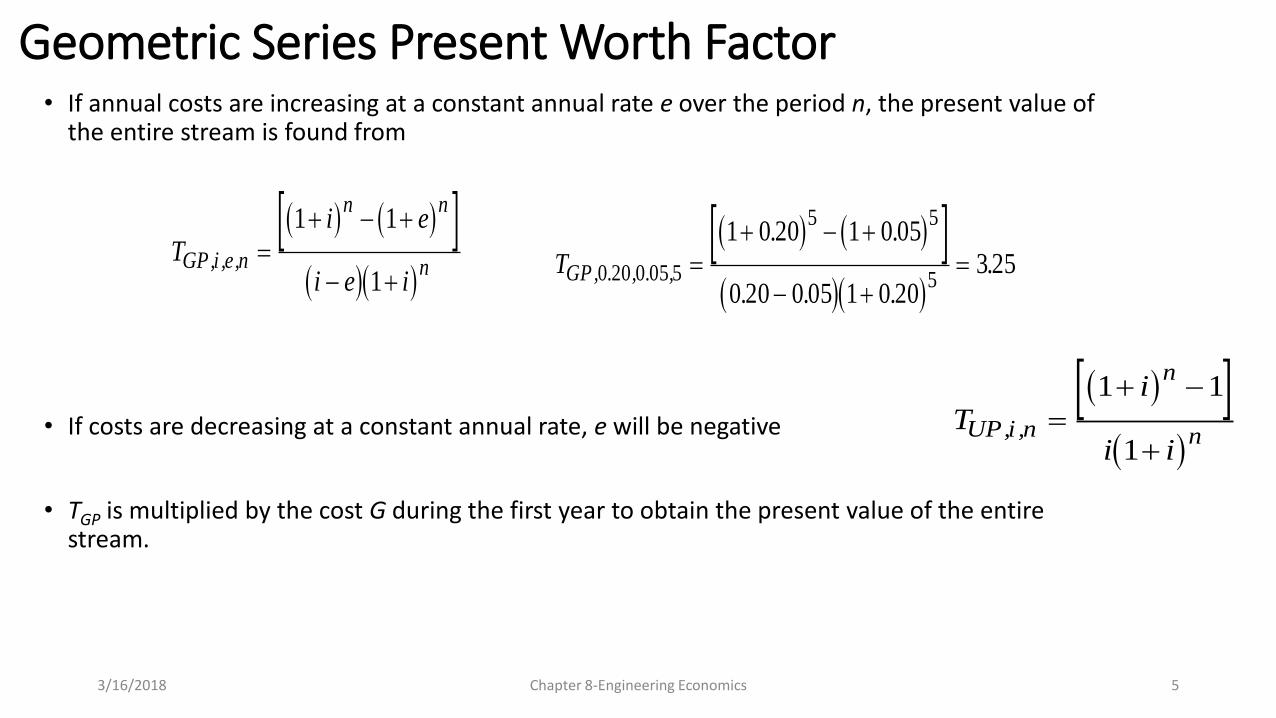
Geometric Series Present Worth Factor• If annual costs are increasing at a constant annual rate e over the period n, the present value of

the entire stream is found from

• If costs are decreasing at a constant annual rate, e will be negative

• TGP is multiplied by the cost G during the first year to obtain the present value of the entire stream.

Ti e

i e iGP i e n

n n

n, , ,

1 1

1

TGP, . , . ,

. .

. . ..0 20 0 05 5

5 5

5

1 0 20 1 0 05

0 20 0 05 1 0 203 25

Ti

i iUP i n

n

n, ,

1 1

1


Present Value Calculation Including TGP ($1,000)• Use discount rate i=0.20

Select Blaylock since the Net Present Value is lower than for Ajax.

Ajax Blaylock

Future/

Annual

Value

Present

Value

Future/

Annual

Value

Present

Value

Initial Cost 30.00 20.00

Rebuilding at End of 3rd year

TFP, . , .0 20 3 0577

- - 3.00 1.73

Salvage Value

TFP, . , .0 20 5 0 403

-4.00 -1.61 - -

Maintenance

TUP, . , .0 20 5 2 99

1.00 2.99 2.00 5.98

Productivity Benefit

TUP, . , .0 20 5 2 99

-0.50 -1.50 - -

Electricity

TGP, . , . , .0 20 0 05 5 325

3.00 9.75 3.50 11.37

Total Present Value Of Costs 39.63 39.08

Ti e

i e iGP i e n

n n

n, , ,

1 1

1

Ti

i iUP i n

n

n, ,

1 1

1

T iFP i nn

, ,

1


Annualized Cost Analysis• Instead of converting all costs to

their equivalent present value, we could instead convert all costs to their equivalent annual value.

• Although the numerical results of the two methods will be different, the least cost alternative using the present value method will also be the least cost alternative using the annualized cost method.

• Capital Recovery Factor

• Sinking Fund Factor

• Generalized Sinking Fund Factor

• Geometric Series Sinking Fund Factor

T

T

i i

iPU i n

UP i n

n

n, ,, ,

1 1

1 1

T

i

iFU i n n, ,

1 1

Ti i e

i i eGU i n

n n

n, ,

1 1

1 1

T

i i

iFU i n

n m

n, ,

1

1 1


Annualized Cost Analysis Ajax Blaylock

Future/

Present

Value

Annual

Value

Future/

Present

Value

Annual

Value

Initial Cost

TPU , . , .0 2 5 0 334

30.00 10.02 20.00 6.68

Rebuilding at End of 3rd year

TFU , . , , .0 2 5 3 0194

- - 3.00 0.58

Salvage Value

TFU , . , .0 2 5 0134

-4.00 -0.54 - -

Maintenance 1.00 2.00

Productivity Benefit -0.50 - -

Electricity

TGU , . , . , .0 2 0 05 5 1086

3.00 3.26 3.50 3.80

Total Equivalent Annual Costs 13.24 13.06

• Capital Recovery Factor

Occur initially (capital)

• Sinking Fund Factor

Occurs downstream (recovery)

• Generalized Sinking Fund Factor

Occurs downstream (rebuilding where m=3)

• Geometric Series Sinking Fund Factor

Geometrically increasing transaction (electricity)


Variations to Basic Engineering Economics Problem

• Unequal lifetimes

• Effect of taxes

• Non-uniform downstream transactions

• Accounting for inflation

• Downstream transactions occurring other than at end of year

• Long project lifetimes


Example of Unequal Lifetimes Problem

Ajax (n=6) Blaylock (n=4)

($1000) ($1000)

Future/

Annual

Value

Present

Value

Future/

Annual

Value

Present

Value

Initial cost - 30.00 - 20.00

Salvage value

33506200 .T ,.,FP

-4.00 -1.34 - -

Maintenance

32636200 .T ,.,UP

1.00 3.33 - -

58924200 .T ,.,UP - - 2.00 5.18

Electricity

67536050200 .T ,.,.,GP

3.00 11.02 - -

75924050200 .T ,.,.,GP - - 3.50 9.66

Total present value of costs 43.01 34.84

• Modified Ajax/Blaylock problem• n(Ajax)=6 n(Blaylock)=4• no rebuilding• no productivity benefit

• Table shows the regular calculation of the decision making process• However if you look at ajax electricity Vs

blaylock electricity, Ajax is more expensive eventhough it consumes less power

• Because it has a longer life• This is unfair

• Alternatively we can do the process for 4 years• But this will be against Ajax as well


Three Approaches to Dealing with Unequal Lifetimes

• Multiple Lifetimes

• Annualized Costs

• Conversion of Present Values

T

T

i i

iPU i n

UP i n

n

n, ,, ,

1 1

1 1

T

i

iFU i n n, ,

1 1

Ti i e

i i eGU i n

n n

n, ,

1 1

1 1


Present Value Calculation for Common Multiple of Lifetimes (n=12)

• Modified Ajax/Blaylock problem• n(Ajax)=6 n(Blaylock)=4

• no rebuilding

• no productivity benefit

• Multiple Lifetimes• Select a analysis period common to lifetime

of both.

• In this case, 4 and 6 years, common term will be 12

• Buy Blayblock at end of 4 and 8 years

• Buy Ajax and end of 6 years

• At 12 year period, Ajax is the better choice

Ajax ($1000) Blaylock ($1000)

Future/

Annual

Value

Present

Value

Future/

Annual

Value

Present

Value

Capital Cost (at n=0) 30.00 20.00

Capita Cost (at n1=4)

( TFP, . , .0 2 4 0482 )

20.00 9.64

Capital Cost (at n2=6)

( TFP, . , .0 2 6 0335 )

30.00

10.05

Capital Cost (at n3=8)

( TFP, . , .0 2 8 0233 )

20.00

4.65

Salvage Value (at n2=6)

( TFP, . , .0 2 6 0335 )

-4.00 -1.34 -

Salvage Value (at n4=12)

( TFP, . , .0 2 12 0112 )

-4.00 -0.45

Maintenance

( TUP, . , .0 2 12 4 439 )

1.00 4.44 2.00 8.88

Electricity

( TGP, . , . , .0 2 0 0512 5324 )

3.00 15.97 3.50 18.63



Annualized Value Calculation for Unequal Lifetimes


($1000) ($1000)

Future/

Present

Value

Annual

Value

Future/

Present

Value

Annual

Value

InitialCost

( 3010620 .T ,.,PU )

( 3860420 .T ,.,PU )

30.00

9.02

20.00

7.73

Salvage Value

( 1010620 .T ,.,FU )

-4.00 -0.40 -

Maintenance 1.00 2.00

Electricity

( 1051605020 .T ,.,.,GU )

( 0661405020 .T ,.,.,GU )

3.00

3.32

3.50

3.73


• Modified Ajax/Blaylock problem• n(Ajax)=6 n(Blaylock)=4

• no rebuilding

• no productivity benefit

• Annualized Costs• All costs expressed as equivalent annual

present value costs

• Inverse factors of TUP, TFP, TGP calculated

• No special treatment needed for difference in lifetime

• Buy Ajax and end of 6 years

• At 12 year period, Ajax is the better choice

T

T

i i

iPU i n

UP i n

n

n, ,, ,

1 1

1 1

Ti

iFU i n n, ,

1 1

Ti i e

i i eGU i n

n n

n, ,

1 1

1 1


Conversion of Present Values*

• Third approach is to Convert any Present Value for period n1 into an equivalent Present Value based on another period n2 using

• Convert P(Ajax) from n1=6 to n2=4 and compare to P(Blaylock)

• Since P4 (Ajax) < P4(Blaylock), choose Ajax

• We can also do the same for Blayblock for 6 years and compare as well

2211 n,i,PUnn,i,PUn TPTP

48.33589.293.12)(

93.12301.001.43)(

4,2.0,4

6,2.0,6

XTAjaxP

XTAjaxP

UP

PU


($1000) ($1000)

Future/

Annual

Value

Present

Value

Future/

Annual

Value

Present

Value

Initial cost - 30.00 - 20.00

Salvage value

33506200 .T ,.,FP

-4.00 -1.34 - -

Maintenance

32636200 .T ,.,UP

1.00 3.33 - -

58924200 .T ,.,UP - - 2.00 5.18

Electricity

67536050200 .T ,.,.,GP

3.00 11.02 - -

75924050200 .T ,.,.,GP - - 3.50 9.66

Total present value of costs 43.01 34.84

T

T

i i

iPU i n

UP i n

n

n, ,, ,

1 1

1 1


The Effect of Taxes

TotalIncome

OperatingExpenses

Depreciation

Taxable Income

Taxes

• Corporation subject to income taxes and type of expense have an effect on the tax rate (mortgage Vs.rental)

• So economic attraction of design options may be influenced

• Figure shows total income on the big block and companies can take deductions on the said income• Operating expenses (payroll, electricity, utility bills etc

• Depreciation (industrial equipment loosing value over time)

• There are different methods of calculating depreciation

• Taxable income is total income – the detections (operating + depreciation)


MACRS Depreciation Schedule Depreciation Period (years)

Year 3 5 7 10 15

1 0.333 0.200 0.143 0.100 0.050

2 0.445 0.320 0.245 0.180 0.095

3 0.148 0.192 0.175 0.144 0.095

4 0.074 0.115 0.125 0.115 0.077

5 0.115 0.089 0.092 0.069

6 0.058 0.089 0.074 0.062

7 0.089 0.066 0.059

8 0.045 0.066 0.059

9 0.065 0.059

10 0.065 0.059

11 0.033 0.059

12-15 0.059

16 0.030

• Depreciation has two components

• Telephone (15 years) computer (5 years)

• Modified Accelerated Cost Recovery System

• % of initial investment that can be depreciated using MARCS shown in table

• Assumed as investments made in the middle of the year, so half year at first and half year after the depreciation period is over

• The total for each adds up to one (means, entire investment is depreciated at the end of the period, even though there might be some salvage value remaining

• When you consider the difference between initial investment and salvage value and divide it over the depreciation period, this is called the Straight line approach


Marginal Tax Rates

Taxable Income Marginal Tax Rates

< 50,000 0.15

50,000 - 75,000 0.25

75,000 - 100,000 0.34

100,000 - 335,000 0.39

335,000 - 10,000,000 0.34

10,000,000 - 15,000,000 0.35

15,000,000 - 18,333,333 0.38

>18,333,333 0.35

• Once we know the depreciation that we can get for that year, we have to apply the tax reate to the allowable depreciation

• This will determine the tax implications of the capital cost of various design alternatives

• Marginal tax rates shown in table


Including Income Tax Effects in Economic Analysis(assume 34% tax bracket and MACRS depreciation schedule with n=5)

Ajax Blaylock

Fut./Ann.Val

.

Pres.

Val.

Fut,/Ann.Val

.

Pres.

Val.

Initial Cost 30.00 30.00 20.00 20.00

Rebuilding at End of 3rd year (TFP,0.2,3

= 0.577)

- - 3.00 1.73

Salvage Value (TFP,0.2,5 = 0.403) -4.00 -1.61 - -

Maintenance (TUP,0.2,5 = 2.99) 1.00 2.99 2.00 5.98

Productivity Benefit (TUP,0.2,5 = 2.99) -0.50 -1.50 - -

Electricity (TGP,0.2,0.05,5 = 3.25) 3.00 9.75 3.50 11.37

Depreciation

1st year @ 0.200 -6.00 -4.00

2nd year @ 0.320 -9.60 -6.40

3rd year @ 0.192 -5.76 -3.84

4th year @ 0.115 -3.45 -2.30

5th year @ 0.115 -3.45 -2.30

6th year @ 0.058 -1.74 -1.16

Tax Benefits from Deprec. @ 0.34

1st year(TFP,0.2,1=0.833) -2.04 -1.70 -1.36 -1.13

2nd year (TFP,0.2,2=0.694) -3.26 -2.26 -2.18 -1.51

3rd year (TFP,0.2,3=0.579) -1.96 -1.13 -1.31 -0.76

4th year (TFP,0.2,4=0.482) -1.17 -0.56 -0.78 -0.38

5th year (TFP,0.2,5=0.402) -1.17 -0.47 -0.78 -0.31

6th year (TFP,0.2,6=0.335) -0.59 -0.20 -0.39 -0.13

Tax Benefits from Maint.+Rebuild.+Elec.

@ 0.34

-4.33 -6.49

Tax Burdens from Product.+ Salv. @ 0.34 1.06


Depreciation for the Ajax motors is based on neglecting salvage value. Assume no depreciation allowed for

rebuilding Blaylock motors.

• Top half of the table is exactly the same as before where we calculate present cost

• % calculated using MACRS at 5 years

• assumed company income is 500000 usd (so 34% tax rate)

• Tax benefit of Depreciation is negative

• Maintenance, rebuild and electricity are operating expenses so direct apply 34% negative again (tax benefit)

• Production and salvage cost incur payment of taxes so hence they are kept positive

• Considering the taxes, Blayblock is the better alternative


Example 8.7.1

• You recommend spending $10,000 on equipment that will increase sales of your product by $1,000 a year and reduce annual operating costs by $800. The equipment has a 10 year lifetime but can be depreciated in three years according to MACRS. Your company uses a 10% discount rate and is in the 25% tax bracket.

• What is the pretax present value of this investment?

• What is the after-tax present value of this investment?


Future/Annual Present

Initial Cost -10,000

Additional annual income TUP,0.1,10 = 6.145 1,000 6,145

Annual savings in operating costs TUP,0.1,10 = 6.145 800 4,916

Pre-tax present value 1,061

Additional tax on additional income rate = 0.25 -1,536

Lost tax deduction on operating costs rate = 0.25 -1,229

Depreciation in year 1 on initial cost 0.333 3,330



Depreciation in year 4 on initial cost 0.074 740

Tax benefits of depreciation in year 1 rate = 0.25 833

Tax benefits of depreciation in year 2 rate = 0.25 1,113



Discounted tax benefits of depr. in year 1 TFP,0.1,1 = 0.909 757




After-Tax Present Value 376

• Pretax calculations show 10 years of additional income and reductions in operating costs when discounted at 10%

• Pretax present value is 1061

• Tax on additional income (6145*.25)

• Tax loss due to reduction in operating cost (4916*0.25)

• Since happen each year, applied directly to present cost

• Depreciation from MACRS table and tax benefit from depreciation

• These values converted to present value using TFP rule

• This gives the after tax present value as 376

Example 8.7.1

Ti

i iUP i n

n

n, ,

1 1

1 T iFP i n

n, ,

1


Cost Estimate for Machining Operation

Category Cost ($)

Feed 1.48

Rapid Traverse 0.11

Load and unload 0.92

Setup 0.43

Tool change 0.49

Tool depreciation 0.13

Tool resharpening 1.48

Rebrazing 0.16

Tip cost 0.10

Grind wheel 0.02

Total $5.33

• For design projects, we need calculation of fabrication costs

• They depend on material being machined, equipment used, tool, operation and rate at which it is performed, desired tolerances, surface finish, and labor

• As example, if we want to consider turning a 3.5” dia 19” long shaft on a lathe using a brazed carbide tool. Shaft is 430 steel

• Cost is summarized in the table. And each cost in itself a detailed calculation

• Tool change cost can be calculated from


Costs and profit

• After calculating the direct and indirect costs, when you provide the customer, you also need to take into account other factors like • Time spent on design, selecting hardware etc

• Man hour * hourly wage * benefits

• Then indirect cost like overheads, utility, telephone, power, etc

• In addition, the company needs to make profit. It could be a % of total costs

• Moreover, an economic safety factor to handle unexpected fluctuations

DECISION MAKING

Last column, normalized such that the total weightage is 1 (cost is 2/6 = 0.3333)

Power

Transmission

Between

Parallel Shafts

Geometry

Health &

Safety

Maintenance

Shaft

Configuration

Noise

(b2)

Shock

Protection

(b1,c6,g6)

Size

(c5,g1)

Install and

Replace Easily

(c2)

Lubrication

Requirement

(b5)

Life

Expectancy

(c7,g5)

Separation

Distance Flexible

(c1)

Misalignment

(b6)

Large Separation

Distance

(b3)

Operating

Conditions

Operating

Speed

Operating

Temperature

(c8)

Speed

Flexibility

(g3)

High Speed

Capability

(b4, g2)

Power/Load

Ratings

Slippage/

Creep

(c4)

Bearing

Loads

(c3)

High Torque

Capability

(g4)

Level 1 Level 2 Level 3 Level 4

Using this formula for 15 criteria mentioned in this tree will give 105 comparisons, becomes difficult

So can break it down to level wise pairwise comparisons

As per previous table, if traditional normalization is used, there is no weightage for recyclability or it has no relevance as a criteria. Other method to do this is use weighted criteria

Start with level 1. 1 criteria so K is 1. Level 2, 5 criteria, divide K such that and since K in level 1 is 1, w is same as K

For level 3 however, k within the group is 1 but w will be the product of K in level 3 and w in level 2 for size it is .25*.1=.025

For level 4 however, k within the group is 1 but w will be the product of K in level 4 and w in level 3 for speed flexibility it is .3*.162=.049

𝑖𝑛 𝑔𝑟𝑜𝑢𝑝

𝑘 = 1

K=1, W=1

K=.5, W=.5

K=.2, W=.1

K=.4, W=.2

K=.4, W=.2

K=.25, W=.25 K=.25, W=.25

K=.75, W=.19

K=.25, W=.06

1A

2A

3A

3B

3C

2B 2C

3D

3E

Documents

Mechanical Engineering Design Project