Embed Size (px)
Citation preview
THÈSE NO 3089 (2004)
ÉCOLE POLYTECHNIQUE FÉDÉRALE DE LAUSANNE
PRÉSENTÉE À LA FACULTÉ SCIENCES DE BASE
Institut de physique de la matière complexe
SECTION DE PHYSIQUE
POUR L'OBTENTION DU GRADE DE DOCTEUR ÈS SCIENCES
PAR
ingénieur physicien, Université de Zagreb, Croatieet de nationalité croate
acceptée sur proposition du jury:
Prof. W. Benoit, directeur de thèseProf. G. Kostorz, rapporteur
Dr D. Mari, rapporteurProf. C. Prioul, rapporteurDr M. Weller, rapporteur
Lausanne, EPFL2004
MECHANICAL PROPERTIES AND MICROSTRUCTUREOF A HIGH CARBON STEEL
Iva TKALCEC

Abstract
This work is focussed on a high carbon tool steel used for the production of files. The mechan-ical properties of the files depend on a hardening thermal treatment that produces a martensiticstructure. Thus, the motivation for this work is technological: we want to understand the effectsof two types of thermal treatment on the file’s mechanical properties. The first is a traditionalthermal treatment in a cyanide bath (CN), while the other is performed in a conveyor belt fur-nace (BF). The files resulting from BF treatment have sometimes a poorer performance. Inorder to improve the quality of BF files, we study the relationship between the mechanicalproperties and the microstructure resulting from a particular thermal treatment.
Transmission electron microscopy does not reveal a change in the microstructure produced bydifferent thermal treatments, yet it does permit visualization of the complex material micro-structure, consisting of a martensitic matrix with embedded carbides. On the other hand, ther-moelectric power measurements allow a differentiation between CN and BF files in a fast andnon-destructive manner: the measurements performed on the whole files show that the ther-mopower of BF files is lower. This result is attributed to a higher concentration of carbon sol-uted in the martensitic matrix. The yield stress and compression strength determined bycompression testing, as well as the hardness measured by nanoindentation, are higher for thebulk of BF files, emphasizing the importance of soluted carbon in hardening the martensite.
The mobility of point defects and dislocations, and their interaction, are studied by mechanicalspectroscopy. The martensitic structure is characterized by a rich internal friction spectrumcomprising several overlapping relaxation and material transformation peaks. The internal fric-tion measured at room temperature is related to an athermal background due to the interactionbetween soluted carbon and dislocations. This background is higher for BF files. The internalfriction spectrum indicates that, upon heating above 375 K, the material structure irreversiblychanges due to tempering processes.
Tempering effects on the material are studied combining several experimental techniques. Afirst stage of tempering, observed by differential scanning calorimetry, starts around 375 K andis related to carbon precipitation in the form of transition carbides. At this temperature, thethermopower and Young’s modulus increase, and the internal friction and hardness decrease,implying that all these quantities are sensitive to soluted carbon. The hardness continuouslydecreases with tempering and no precipitation hardening is observed. A second stage of tem-pering is observed around 525 K, leading to cementite precipitation.
X-ray diffraction allows quantitative determination of the concentration of carbon in solidsolution by measuring the tetragonality of the martensite lattice. The evolution of carbon con-tent during tempering is compared to the evolution of internal friction and thermoelectricpower revealing a strong correlation between these quantities. Internal friction measured atroom temperature is directly proportional to the carbon content.
The measurement of the concentration of carbon by X-ray diffraction is used to determine thevariation of carbon content in the file profile. Thermopower measurements indicate that BFfiles have a lower concentration of carbon in the teeth than in the bulk, while the opposite isfound for CN files. This is confirmed by X-ray diffraction. Moreover, diffraction performed onthe very surface of the teeth reveals a lower carbon concentration in BF than in CN files teeth,which is probably the origin of their lesser performance.
It can be concluded that the concentration of carbon in solid solution in martensite is responsi-ble for the steel’s hardness and therefore for its resistance to wear.

Version abrégée
Cette étude concerne principalement un acier à outils à haute teneur en carbone utilisé pour laproduction de limes. Les propriétés mécaniques des limes dépendent du traitement thermiquede trempe qui produit une structure martensitique. Ainsi, la motivation de ce travail est d’abordtechnologique : il s’agit de comprendre les effets de deux types de traitement thermique deslimes sur leurs propriétés mécaniques. Le premier est un traitement thermique traditionneldans un bain de sel de cyanure (CN), tandis que le deuxième est effectué dans un four à bande(BF). Les performances des limes issues du traitement en four à bande sont parfois de qualitéinférieure. Pour améliorer la qualité des limes de type BF, on étudie le lien entre les propriétésmécaniques et les microstructures issues d’un traitement thermique particulier.
La microscopie électronique à transmission ne montre pas de différences de microstructureentre traitements thermiques, mais elle permet de visualiser la microstructure complexe dumatériau, formée d’une matrice martensitique entourant des carbures. D’autre part, la mesuredu pouvoir thermoélectrique permet de différencier entre les limes de type CN et les limes detype BF de manière non-destructive. Des mesures effectuées sur des limes complètes montrenten effet que le pouvoir thermoélectrique des limes BF est inférieur. Ce résultat est attribué àune concentration supérieure du carbone en solution dans la matrice martensitique. La limiteélastique et la résistance mécanique déterminées dans les tests de compression, de même que ladureté mesurée par nano-indentation, sont supérieures dans les limes de type BF, mettant ainsien évidence l’importance du carbone en solution dans le durcissement de la martensite.
La mobilité des défauts ponctuels et des dislocations, ainsi que leurs interactions, sont étudiéespar spectroscopie mécanique. La structure martensitique est caractérisée par un spectre de frot-tement intérieur très riche, résultant de la superposition de plusieurs pics de relaxation et dephénomènes de transformations du matériau. Le frottement intérieur mesuré à températureambiante est corrélé avec un fond athermique dû à l’interaction entre dislocations et carbone ensolution. Le spectre de frottement intérieur indique qu’après chauffage au-dessus de 375 K lastructure du matériau change de manière irréversible à cause du revenu de l’acier.
Les effets des revenus sur le matériau sont étudiés en combinant différentes techniques expéri-mentales. Un premier stade de revenu, observé par calorimétrie différentielle, commenceautour de 375 K et est déterminé par la précipitation du carbone sous forme de carbures detransition. A cette température, le pouvoir thermoélectrique et le module de Young augmentent,tandis que le frottement interne et la dureté diminuent, ce qui implique que toutes ces quantitéssont sensibles au carbone en solution. La dureté décroît de manière continue avec le revenu etl’on n’observe pas de durcissement par précipitation. Un deuxième stade de revenu est observéà 525 K, conduisant à la précipitation de cémentite.
La diffraction de rayons X permet de déterminer de manière quantitative la concentration decarbone en solution solide en mesurant la tétragonalité du réseau cristallin de la martensite.L’évolution de la teneur en carbone pendant le revenu est comparée avec l’évolution du frotte-ment intérieur et du pouvoir thermoélectrique, montrant une étroite corrélation entre ces quan-tités. Le frottement intérieur mesuré à température ambiante est directement proportionnel à laconcentration du carbone.
La diffraction de rayons X nous a permis également de déterminer le profil de concentration ducarbone dans l’épaisseur de la lime. Les mesures de pouvoir thermoélectrique indiquent queles limes de type BF ont une concentration de carbone supérieure à l’intérieur de la lime tandisque l’effet opposé est présent dans les limes de type CN. Ceci est confirmé par diffraction de

rayons X. D’ailleurs, la diffraction effectuée à la surface des dents montre que la concentrationde carbone dans les dents des limes de type BF est inférieure à celle des dents des limes de typeCN, ce qui est probablement à l’origine de leur moindre performance.
On peut conclure que la concentration de carbone en solution solide dans la martensite est lasource principale de la dureté de l’acier et par conséquent de sa résistance à l’usure.
Contents
Introduction . . . . . . . . . . . . . . . . . . . . . . . . . . . . . . . . . . . . . . . . . . . . . . . 1
1. Martensitic steel: basic description . . . . . . . . . . . . . . . . . . . . . . . . . . 5
1.1 Crystal forms and interstitial solubility of iron: iron-carbon phase diagram . . . 5
1.2 Martensitic transformation . . . . . . . . . . . . . . . . . . . . . . . . . . . . . . . . . . . . . . . . . . 6
1.3 Martensite morphology . . . . . . . . . . . . . . . . . . . . . . . . . . . . . . . . . . . . . . . . . . . . . 9
1.4 Aging and tempering of martensite . . . . . . . . . . . . . . . . . . . . . . . . . . . . . . . . . . . . 9
2. Experimental techniques and relevant results from literature . . . . 11
2.1 Thermomechanical treatment during file processing . . . . . . . . . . . . . . . . . . . .11
2.2 Microstructural analysis . . . . . . . . . . . . . . . . . . . . . . . . . . . . . . . . . . . . . . . . . . .11
2.2.1 Transmission electron microscopy . . . . . . . . . . . . . . . . . . . . . . . . . . . . . .112.2.2 Atomic force microscopy . . . . . . . . . . . . . . . . . . . . . . . . . . . . . . . . . . . . . 122.2.3 X-ray diffraction . . . . . . . . . . . . . . . . . . . . . . . . . . . . . . . . . . . . . . . . . . . . . 13
Principles and experimental procedure . . . . . . . . . . . . . . . . . . . . . . . . . . 13Relevant experimental results found in literature . . . . . . . . . . . . . . . . . . 14
2.3 Thermoelectric power . . . . . . . . . . . . . . . . . . . . . . . . . . . . . . . . . . . . . . . . . . . . 15
2.3.1 Principles and experimental procedure . . . . . . . . . . . . . . . . . . . . . . . . . . . 152.3.2 Relevant experimental results found in literature . . . . . . . . . . . . . . . . . . . 17
2.4 Mechanical tests . . . . . . . . . . . . . . . . . . . . . . . . . . . . . . . . . . . . . . . . . . . . . . . . 19
2.4.1 Compression . . . . . . . . . . . . . . . . . . . . . . . . . . . . . . . . . . . . . . . . . . . . . . 192.4.2 Nanoindentation . . . . . . . . . . . . . . . . . . . . . . . . . . . . . . . . . . . . . . . . . . . 20
2.5 Mechanical spectroscopy . . . . . . . . . . . . . . . . . . . . . . . . . . . . . . . . . . . . . . . . . 22
2.5.1 Phenomenology and definitions . . . . . . . . . . . . . . . . . . . . . . . . . . . . . . . 222.5.2 Experimental installations . . . . . . . . . . . . . . . . . . . . . . . . . . . . . . . . . . . . 25
Free-free vibrating reed installation . . . . . . . . . . . . . . . . . . . . . . . . . . . . 26Inverted torsion pendulum . . . . . . . . . . . . . . . . . . . . . . . . . . . . . . . . . . . . 27
2.5.3 Relevant experimental results found in literature . . . . . . . . . . . . . . . . . . 28
2.6 Differential scanning calorimetry . . . . . . . . . . . . . . . . . . . . . . . . . . . . . . . . . . 32
2.6.1 Principles and experimental procedure. . . . . . . . . . . . . . . . . . . . . . . . . . . . 322.6.2 Relevant experimental results found in literature . . . . . . . . . . . . . . . . . . . 33
3. Material properties at room temperature . . . . . . . . . . . . . . . . . . . . 35
3.1 Microstructure . . . . . . . . . . . . . . . . . . . . . . . . . . . . . . . . . . . . . . . . . . . . . . . . . . 35
3.1.1 Chemical composition . . . . . . . . . . . . . . . . . . . . . . . . . . . . . . . . . . . . . . . 353.1.2 Atomic force microscopy . . . . . . . . . . . . . . . . . . . . . . . . . . . . . . . . . . . . 353.1.3 Transmission electron microscopy . . . . . . . . . . . . . . . . . . . . . . . . . . . . . 36
3.2 Thermoelectric power . . . . . . . . . . . . . . . . . . . . . . . . . . . . . . . . . . . . . . . . . . . . 41
Contents
3.3 Mechanical tests . . . . . . . . . . . . . . . . . . . . . . . . . . . . . . . . . . . . . . . . . . . . . . . . 46
3.3.1 Compression . . . . . . . . . . . . . . . . . . . . . . . . . . . . . . . . . . . . . . . . . . . . . . 463.3.2 Nanoindentation . . . . . . . . . . . . . . . . . . . . . . . . . . . . . . . . . . . . . . . . . . . 46
3.4 Conclusions . . . . . . . . . . . . . . . . . . . . . . . . . . . . . . . . . . . . . . . . . . . . . . . . . . . . 48
4. Mechanical spectroscopy . . . . . . . . . . . . . . . . . . . . . . . . . . . . . . . . . 51
4.1 Temperature spectra . . . . . . . . . . . . . . . . . . . . . . . . . . . . . . . . . . . . . . . . . . . . . 51
4.1.1 High and low frequency spectra for martensite . . . . . . . . . . . . . . . . . . . 514.1.2 Evolution of martensitic spectra with ageing and tempering . . . . . . . . . 554.1.3 Internal friction for tempered martensitic, ferritic and bainitic structure 614.1.4 Effects of cold work on deeply tempered martensite and ferrite . . . . . . . 614.1.5 Difference between thermal treatments of files . . . . . . . . . . . . . . . . . . . . 63
4.2 Discussion . . . . . . . . . . . . . . . . . . . . . . . . . . . . . . . . . . . . . . . . . . . . . . . . . . . . . 65
4.3 Conclusions . . . . . . . . . . . . . . . . . . . . . . . . . . . . . . . . . . . . . . . . . . . . . . . . . . . . 73
5. Tempering effects . . . . . . . . . . . . . . . . . . . . . . . . . . . . . . . . . . . . . . . 75
5.1 Differential scanning calorimetry . . . . . . . . . . . . . . . . . . . . . . . . . . . . . . . . . . 75
5.2 Transmission electron microscopy . . . . . . . . . . . . . . . . . . . . . . . . . . . . . . . . . . 76
5.3 Thermoelectric power . . . . . . . . . . . . . . . . . . . . . . . . . . . . . . . . . . . . . . . . . . . . 77
5.4 Internal friction . . . . . . . . . . . . . . . . . . . . . . . . . . . . . . . . . . . . . . . . . . . . . . . . . 80
5.5 Young’s modulus . . . . . . . . . . . . . . . . . . . . . . . . . . . . . . . . . . . . . . . . . . . . . . . . 80
5.6 Nanoindentation . . . . . . . . . . . . . . . . . . . . . . . . . . . . . . . . . . . . . . . . . . . . . . . . 81
5.7 Discussion . . . . . . . . . . . . . . . . . . . . . . . . . . . . . . . . . . . . . . . . . . . . . . . . . . . . . 82
5.8 Conclusions . . . . . . . . . . . . . . . . . . . . . . . . . . . . . . . . . . . . . . . . . . . . . . . . . . . . 85
6. X-ray diffraction . . . . . . . . . . . . . . . . . . . . . . . . . . . . . . . . . . . . . . . . 87
6.1 Tempering effects on carbon concentration . . . . . . . . . . . . . . . . . . . . . . . . . . . 87
6.1.1 Carbon content fitting . . . . . . . . . . . . . . . . . . . . . . . . . . . . . . . . . . . . . . . . 886.1.2 Correlation with TEP and internal friction . . . . . . . . . . . . . . . . . . . . . . . . 90
6.2 Variation of the amount of carbon in solid solution within a file . . . . . . . . . . 93
6.2.1 Experiments on the bulk and whole teeth of files . . . . . . . . . . . . . . . . . . . . 936.2.2 Experiments on the surface of file teeth . . . . . . . . . . . . . . . . . . . . . . . . . . . 95
6.3 Conclusions . . . . . . . . . . . . . . . . . . . . . . . . . . . . . . . . . . . . . . . . . . . . . . . . . . . . 97
7. Conclusion . . . . . . . . . . . . . . . . . . . . . . . . . . . . . . . . . . . . . . . . . . . . . 99
Bibliography . . . . . . . . . . . . . . . . . . . . . . . . . . . . . . . . . . . . . . . . . . . . . . 103
Acknowledgments . . . . . . . . . . . . . . . . . . . . . . . . . . . . . . . . . . . . . . . . . . 109
1
Introduction
Despite constant development of new materials, steel is still one of the most reliable, mostused, and most important materials of today. Depending on the chemical composition and thethermomechanical processing history during the manufacturing process, its mechanical prop-erties can vary tremendously, covering an extensive range of strength, toughness and ductility.Steel can also be relatively cheaply manufactured in large quantities to very precise specifica-tions. Therefore, it is not surprising that irons and steels account for over 80% by weight of thealloys used in industry [Honeycombe 1980]. Carbon steels are widespread materials becauseof the possibility to induce in them, by means of a rapid quenching, an extremely hard phase:martensite. Due to the complexity of the microstructure of martensitic carbon steels, their char-acterization often remains empirical.
The material in focus of this research is a high carbon tool steel used for the production of files.After shaping, the files are heated above the temperature of austenitization and then quenched.Traditionally, this heat treatment giving the necessary hardness and grip to the files, is per-formed manually in a cyanide salt bath. This process has a low productivity, it requires spe-cially trained personnel and the costs of ecologically safe elimination of the waste are veryhigh. The alternative is a heat treatment in a conveyor belt furnace, but the resulting quality isnot always satisfactory. Therefore, the technological objective of this work is to understand theeffects of thermal treatment on the mechanical properties of carbon steel designated for theproduction of files. The research is performed in collaboration with one of the most importantfile producers in the world, UMV Vallorbe, Switzerland.
The properties of interest for a file user are the grip (bite) of the file and its longevity. Each fileproduced in UMV Vallorbe passes through a quality control where the grip of the file is testedmanually by an experienced staff. This process is rather subjective. A more quantitative mea-sure for the mechanical performance can be obtained by tracing the filing behavior under con-trolled conditions (normal force and stroke speed). An instrument developed by UMV enablesthe measurement of the force necessary to move a file on a test material, i.e. the grip, and themass of the test material removed by that action. The later quantity can be related to a file lon-gevity if the test is performed during long enough time: after sufficient number of strokes thedegradation of the file is reflected in the reduced increase of the total mass of the test materialremoved by filing. The results of a test performed on both cyanide bath (CN) and conveyor beltfurnace (BF) treated files for a total number of 3000 strokes are presented in fig. 1 and fig. 2.As seen from the graphs, some types of files clearly show different performances. In fig. 1, weobserve that the files treated traditionally have a superior grip (with the exception of the first
Introduction
2
few strokes). The grip is diminishing with the use, but this deterioration is more pronouncedfor the files treated in the conveyor belt furnace. Moreover, CN treated files keep removing thetest material after 3000 strokes with almost the same efficiency as when they were new (fig. 2).On the contrary, although not showing a great difference at the beginning (up to 500 strokes),BF treated files with further use remove less and less material, reaching after 3000 strokes astate when the material is no longer removed by filing.
The files have the same initial chemical composition and by traditional testing methods(Vicker’s hardness tests, observation of structure by optical or SEM microscope) the filesresulting from two types of thermal treatment cannot be distinguished. Therefore, a more sci-entific approach, using various experimental techniques is necessary to relate macroscopicmechanical properties of steel to the microstructure emanating from a particular heat treat-ment. This thesis will show that the carbon in solid solution is responsible for the resistance ofthe material to deformation, in particular its hardness.
Because of the huge industrial and economical importance of steel and also its great complex-ity, a vast amount of literature exists covering the topic. Hence it is not possible to condensethat huge amount of information in a traditional thesis chapter entitled “Bibliography”. Chap-ter 1 aims to briefly describe the fundamental terminology related to martensitic steel startingfrom crystal structure and carbon solubility in pure iron, martensitic transformation and result-ing martensite morphology.
Several experimental techniques are used in this work. Microstructural analysis is made com-plementing transmission electron microscopy (TEM), atomic force microscopy (AFM) and X-ray diffraction. Thermoelectric power is also used as a very sensitive probe of the microstruc-tural state of the material. The mobility of defects (point defects and dislocations) and theirinteraction is studied by mechanical spectroscopy. Mechanical properties are investigated bynanoindentation and compression testing. Finally, differential scanning calorimetry is used forthermal analysis. A short description of each technique and the used parameters is given inChapter 2 together with basic results obtained by other authors.
FIGURE 1.
The force of the grip of the file as afunction of the number of strokes performed on atest material under controlled conditions. The forcedecreases with use, but the decrease is smaller forCN files.
FIGURE 2.
The mass of the test material removed byfiling as a function of the number of strokes. CNfiles continue to remove the test material after 3000strokes with almost the same rate as when new. BFfiles show deterioration starting from 500 strokes,and after 3000 strokes material is no longerremoved.
10
15
20
25
30
35
40
45
0 500 1000 1500 2000 2500 3000Number of strokes
Forc
e [N
]
BF
CN
0
1
2
3
4
5
6
7
8
9
10
0 500 1000 1500 2000 2500 3000 3500Number of strokes
Mas
s of
mat
eria
l rem
oved
[g]
BF
CN
Introduction
3
Experimental results are presented in four distinct chapters ending with a discussion and con-clusions. Chapter 3 contains the description of the material properties at room temperature,showing the base differences between CN and BF treated files. A comparison of the measure-ments of thermoelectric power and the mechanical tests emphasizes the importance of the car-bon in solid solution. Mechanical spectroscopy is thus used to get a better insight into theinteractions of soluted atoms and dislocations and their mobility. An extensive study of theinternal friction spectra is presented in Chapter 4. The internal friction spectra indicate that thematerial microstructure continuously changes at temperatures higher than 375 K. The effectsof tempering, examined in more detail with a wide range of techniques, are described in Chap-ter 5. Finally, Chapter 6 contains the results of X-ray diffraction experiments, giving an expla-nation for the differences in mechanical properties resulting from the two types of thermaltreatment and material evolution during tempering.
The scientific conclusions are summarized in Chapter 7.

5
CHAPTER 1
Martensitic steel: basic description
There are evidences of use of meteoritic iron as early as around 2700 BC in Egypt, but it tookanother one and a half millennia for iron to start to replace bronze around 1200 BC [Maddin1992]. In effect, pure iron has a lot of disadvantages in comparison with bronze: the meltingtemperature of iron is 1536˚C, which was impossible to reach with the means of that time,therefore it could not have been cast, moreover, it corrodes easily. Although iron ores weremore readily found than tin, which was required in addition to copper for making bronze, itwas necessary to develop hardening processes in order to make iron more appealing. By dis-solving carbon into iron (and thus forming steel) and quenching it to martensite, an immenseimprovement over bronze could be achieved.
The following paragraphs aim to briefly describe the basic terminology used further on in thisthesis. The properties of steel are conditioned by certain properties of pure iron, namely itscrystal structure and other element solubility characteristics. As it suffices to add carbon to ironto form steel, the carbon solubility will be regarded in more detail, without discussing theeffects of other alloying elements. The thermal treatment producing the characteristic steelmorphology will also be shortly discussed.
1.1 Crystal forms and interstitial solubility of iron: iron-carbon phase diagram
Pure iron is polymorphic: depending on temperature, two allotropic phases exist in solid state.One is body centered cubic (bcc) and the other face centered cubic (fcc). The bcc crystallineform (
α
-iron, ferrite) is stable from low temperatures to 910ºC when it transforms to fcc (
γ
-iron, austenite). The austenite remains stable until 1390ºC, and then it reverts to the bcc form,now called
δ
-iron, which is stable until the melting point of 1536˚C. High purity iron is veryweak (the resolved shear stress can be as low as 10 GPa for single-crystals, and 150 GPa forpolycrystalline samples). The ability of iron to accommodate heavy interstitials, namely car-bon and nitrogen, is mostly responsible for hardening effects.
It is interesting that the fcc structure, which is more closely packed than bcc, contains largercavities. The largest voids in the fcc structure are situated at the centers of the cube edges, andare surrounded by six atoms in the form of an octahedron, therefore called octahedral(fig. 1.1a). The radius of the largest sphere fitting in this space is 0.41
r
,
r
being the atomic
Chapter 1
6
radius of iron (1.28 Å). Second largest are tetrahedral interstices (fig. 1.1b), which can accom-modate a sphere up to the radius of 0.23
r
.
The largest cavities (0.29
r
) in the bcc structure are found between two edge and two centralatoms forming a tetrahedron (tetrahedral sites, fig. 1.1d). The second largest (0.15
r
) are octahe-dral sites found at the centers of the cube faces and of the cube edges (fig. 1.1c). The surround-ing atoms form a flattened octahedron.
The atomic radius of a carbon atom in iron is sufficiently small (0.6
r)
to enter the interstitialsites, however with some lattice distortion. The fact that there are larger interstitial cavitiesavailable in the fcc than in the bcc structure explains the much larger solubility of carbon in
γ
than in
α
-iron. The maximum carbon solubility in austenite reaches 2.04 wt.% at 1147ºC, com-pared with 0.02 wt.% in ferrite at 723ºC. These and other equilibrium features are bestdescribed by means of the iron-carbon phase diagram (fig. 1.2). It should be mentioned that thetrue equilibrium exists between iron and graphite (occurring in cast irons with 2-4 wt.% C). Asgraphite is difficult to obtain in steels, the metastable equilibrium between iron and cementiteis considered. Cementite is an iron-carbide with the chemical formula Fe
3
C and an orthorom-bic crystal structure.
The much greater solubility of carbon is reflected in a much larger phase field of austenite thanferrite. For the carbon content higher than 0.008 wt.%,
α
-iron is accompanied by iron carbide.The transformation temperature of 910ºC between austenite and ferrite for pure iron is progres-sively lowered by the addition of carbon to the eutectoid temperature of 723ºC and the eutec-toid composition of 0.8 wt.% C.
1.2 Martensitic transformation
Sufficiently rapid cooling of austenite containing carbon will prevent the formation offerrite + cementite which would happen with adequately slow cooling, i.e. if the diffusion ofcarbon atoms is allowed. The carbon atoms soluted in austenite remain trapped, causing thetetragonal distortion of the bcc lattice and the formation of a very hard metastable phase: mar-tensite. The martensitic transformation in steel is just one example of a more general phenom-enon of martensitic transformations described as shear-dominant, lattice-distortive,diffusionless transformations occurring by nucleation and growth [Olson 1992].
a) b) c) d)
FIGURE 1.1.
Interstitial voids in iron. Octahedral (a) and tetrahedral (b) voids in fcc structure. Octahedral(c) and tetrahedral (d) voids in bcc structure. Taken from [Leslie 1981].
METAL ATOMS
INTERSTICES
Chapter 1
8
The correspondence between austenite and ferrite lattices was first described by Bain. Asshown in the figure 1.4, octahedral interstitial sites in fcc would be converted to c-orientedoctahedral sites in bct. However, to convert this cell to a martensite cell, a contraction of about17% of the c-axis and an expansion of about 12% of the a-axis is necessary (Bain strain). Sucha deformation would require a considerable amount of energy to overcome the potential barrierfor the development of a martensite nucleus in the surrounding austenite. On the contrary,experiments show that the martensitic transformation occurs practically without thermal acti-vation and that it propagates at the a speed close to the speed of sound. The minimization of thestrain energy requires an invariant plane separating the parent and the product phase (undis-torted and unrotated habit plane) and such interfaces are observed experimentally. This meansthat the transformation strains must constitute an invariant plane strain (
S
). The existence of ahabit plane can be achieved by the combination of Bain’s homogeneous shape deformation (
B
)with an inhomogeneous lattice invariant deformation, as for example shear (
P
). All that is thennecessary is to rotate the strained region by a rotation
R
in order to make the habit plane bothundistorted and unrotated. So, mathematically, a martensitic transformation can be representedby the multiplication of three transformation matrices:
.
(1.1)
In general, the indices of the habit plane are irrational. The required shear could result fromdislocation glide (dislocations are found in martensites in high concentrations of 10
11
to10
12
cm
-2
, which is a value found for heavily cold worked metals) producing slip, or fromtwinning. Twinning is facilitated at high carbon concentrations. As a consequence, differentmartensite morphologies can be found depending on the carbon content.
The tetragonal distortion of the ferritic bcc matrix due to the martensitic transformation highlydepends on the carbon content. This dependence of lattice parameters
a
and
c
is described by
(1.2)
(1.3)
where
a
0
is the lattice parameter of bcc iron (2.8663 Å) and
x
is the concentration of carbon inweight percent [Kurdjumov 1976, Cheng 1990].
FIGURE 1.4.
The lattice correspondence for formation of martensite from austenite as described by Bain. Atetragonal unit cell is outlined in austenite. The interstitial atom (black circle) in an octahedral site in fcc ispositioned in the c-oriented octahedral site in bcc. Such tetragonal unit cell has to be compressed along c(about 20%) and expanded along a (about 12%) to be transformed into the martensite unit cell.
S RPB=
[001]α'[001] γ
[010]α'[100]α' [100] γ
[010] γ a a
c
c a0 0.116x+=
a a0 0.013x–=

Martensitic steel: basic description
9
1.3 Martensite morphology
Lath martensite (fig. 1.5a) is normally found in steels with lower concentrations of carbon (upto 0.5 wt.%). The structure units are laths, mostly separated by low angle boundaries, groupedinto packets. The substructure is characterized by a very high concentration of dislocations.Plate martensite (fig. 1.5b) is characteristic for high carbon steels (more than 1.3 wt.%). Thestructure is made of lenticular plates of martensite units, each consisting of fine twins about5 nm apart. These twins gradually merge into an array of dislocations near the periphery of theplate. The microstructure of steels containing carbon in the range 0.5 to 0.8 wt.% is generallycomplicated, with lath martensite, plate martensite and residual, non-transformed austenitecoexisting together (fig. 1.6a). The effect of carbon content on the volume percent of lath andplate martensite, the temperature of the martensitic transformation and the volume percent ofresidual austenite are shown in fig. 1.6b [Speich 1972a].
1.4 Aging and tempering of martensite
Iron-carbon martensite is a metastable structure, and as such it can undergo structural changeseven at low temperature. Historically, the term tempering is used for a process of heating mar-tensitic steels to elevated temperatures so that they become more ductile. The term aging isreferring to the processes that occur during the storage of martensite at room temperature.
The aging and tempering behavior of iron-carbon martensite has been the subject of intensiveinvestigation for more than 60 years and a large amount of literature exists covering the subject
FIGURE 1.5.
a) Microstructure of lath martensite in a steel containing 0.2 wt.% carbon. Laths are usuallyseparated by low angle boundaries and grouped into a packet. b) Plate martensite microstructure found in asteel containing 1.4 wt% carbon, characterized by fine twinning. Taken from [Nishiyama 1978].
FIGURE 1.6.
a) Microstructure of steel containing 0.8 wt.% C. Both lath and plate martensite can bedistinguished [Nishiyama 1978]. b) Effect of carbon content on relative volume percent of lath and platemartensite, M
s
temperature, and volume percent of retained austenite in Fe-C alloys [Speich 1972a].
1µ
a) b)
1µ
a)
1µ
b)
Chapter 1
10
[Schmidtmann 1965, Speich 1969, Speich 1972a, Inoue 1978, Olson 1983, Samuel 1983,Krauss 1984, Chang 1986, Cheng 1988, Mittemeijer 1991, Cheng 1990, Ohmori 1992, Speich1992, Van Genderen 1997, Han 2001]. Research has shown that the decomposition processesare complex and involve many overlapping phenomena. The temperature ranges at which theyoccur are dependent on heating rate, composition and structural details. They can be summa-rized as follows (for iron carbon martensite containing about 1 wt.% C and for heating rates ofthe order of 10 to 20 K/min [Mittemeijer 1991]):
a) Transformation of a part of the retained austenite into martensite between 115 and 215 K
b) Redistribution of carbon atoms (preprecipitation processes) around and slightly above roomtemperature, ascribed to:
i) Segregation of carbon atoms to lattice defects (~0.2 wt.% C).
ii) Transfer of carbon atoms at a/b octahedral interstices to c octahedral interstices
iii) Formation of carbon enrichments in the matrix for the predominant part of the carbonatoms
c) First stage of tempering between 355 and 455 K: precipitation of transition carbides
d) Second stage of tempering between 475 to 625 K: decomposition of retained austenite intoferrite and cementite
e) Third stage of tempering between 525 and 625 K: precipitation of the stable carbide,cementite
f) Recovery of dislocation substructure, recrystallization, grain growth and sphereoidization ofcementite between 600 and 900 K.
11
CHAPTER 2
Experimental techniques and relevant results from literature
This chapter contains a brief description of file processing and experimental methods used inthe course of this work. Significant works from the literature are described in order to illustratethe possibilities of experimental methods to study the mechanical behavior and microstructureof carbon steel martensite.
2.1 Thermomechanical treatment during file processing
The thermomechanical treatment of the material during the file production can be divided intothree operations: normalization, shaping, and hardening. The raw material is first normalizedby annealing for 15 min at 1150 K and subsequent air-cooling, in order to obtain a ferriticstructure with embedded spheroidized carbide particles. Next, the material is machined toobtain the final file form. This shaping is performed in several steps, each involving more orless heavy plastic deformation. The shape of the studied files is approximately rectangular,with the dimensions cm
3
. The teeth, 0.2 mm high with 0.5 mm step size, arecut on two sides. Finally, the thermal treatment producing the hard martensitic phase and thusgiving necessary hardness to the file consists in rapid quenching after about 15 min of austen-itization at 1100 K. The austenitization can be performed either traditionally, in the cyanidesalt bath (CN) or in the conveyor belt furnace (BF) under protective and slightly nitridingatmosphere.
2.2 Microstructural analysis
2.2.1 Transmission electron microscopy
Transmission electron microscopy (TEM) is used with the aim of visualizing the microstruc-ture of the material. Particular attention is dedicated to the study of the martensite morphology,dislocation structure and the presence of residual austenite.
TEM is such a widely used technique that it needs no special presentation. A point that requiresmore attention is the sample preparation method. In order to study the microstructure by TEM,
19 1.4 0.22××
Chapter 2
12
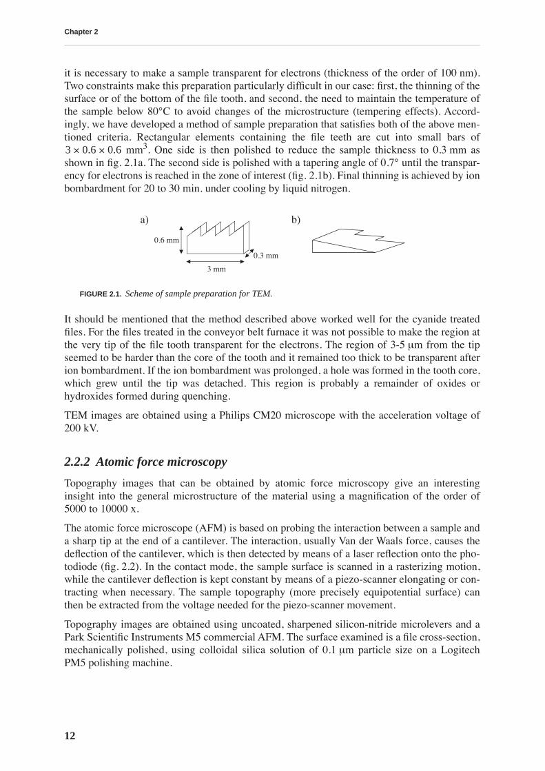
it is necessary to make a sample transparent for electrons (thickness of the order of 100 nm).Two constraints make this preparation particularly difficult in our case: first, the thinning of thesurface or of the bottom of the file tooth, and second, the need to maintain the temperature ofthe sample below 80°C to avoid changes of the microstructure (tempering effects). Accord-ingly, we have developed a method of sample preparation that satisfies both of the above men-tioned criteria. Rectangular elements containing the file teeth are cut into small bars of
mm
3
. One side is then polished to reduce the sample thickness to 0.3 mm asshown in fig. 2.1a. The second side is polished with a tapering angle of 0.7° until the transpar-ency for electrons is reached in the zone of interest (fig. 2.1b). Final thinning is achieved by ionbombardment for 20 to 30 min. under cooling by liquid nitrogen.
It should be mentioned that the method described above worked well for the cyanide treatedfiles. For the files treated in the conveyor belt furnace it was not possible to make the region atthe very tip of the file tooth transparent for the electrons. The region of 3-5
µ
m from the tipseemed to be harder than the core of the tooth and it remained too thick to be transparent afterion bombardment. If the ion bombardment was prolonged, a hole was formed in the tooth core,which grew until the tip was detached. This region is probably a remainder of oxides orhydroxides formed during quenching.
TEM images are obtained using a Philips CM20 microscope with the acceleration voltage of200 kV.
2.2.2 Atomic force microscopy
Topography images that can be obtained by atomic force microscopy give an interestinginsight into the general microstructure of the material using a magnification of the order of5000 to 10000 x.
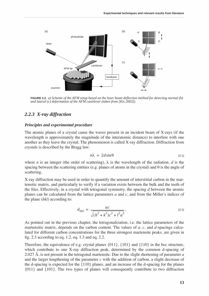
The atomic force microscope (AFM) is based on probing the interaction between a sample anda sharp tip at the end of a cantilever. The interaction, usually Van der Waals force, causes thedeflection of the cantilever, which is then detected by means of a laser reflection onto the pho-todiode (fig. 2.2). In the contact mode, the sample surface is scanned in a rasterizing motion,while the cantilever deflection is kept constant by means of a piezo-scanner elongating or con-tracting when necessary. The sample topography (more precisely equipotential surface) canthen be extracted from the voltage needed for the piezo-scanner movement.
Topography images are obtained using uncoated, sharpened silicon-nitride microlevers and aPark Scientific Instruments M5 commercial AFM. The surface examined is a file cross-section,mechanically polished, using colloidal silica solution of 0.1
µ
m particle size on a LogitechPM5 polishing machine.
FIGURE 2.1.
Scheme of sample preparation for TEM.
3 0.6 0.6××
3 mm
0.6 mm
0.3 mm
a) b)
Experimental techniques and relevant results from literature
13
2.2.3 X-ray diffraction
Principles and experimental procedure
The atomic planes of a crystal cause the waves present in an incident beam of X-rays (if thewavelength is approximately the magnitude of the interatomic distance) to interfere with oneanother as they leave the crystal. The phenomenon is called X-ray diffraction. Diffraction fromcrystals is described by the Bragg law:
(2.1)
where
n
is an integer (the order of scattering),
λ
is the wavelength of the radiation,
d
is thespacing between the scattering entities (e.g. planes of atoms in the crystal) and
θ
is the angle ofscattering.
X-ray diffraction may be used in order to quantify the amount of interstitial carbon in the mar-tensitic matrix, and particularly to verify if a variation exists between the bulk and the teeth ofthe files. Effectively, in a crystal with tetragonal symmetry, the spacing
d
between the atomicplanes can be calculated from the lattice parameters
a
and
c
, and from the Miller’s indices ofthe plane (
hkl)
according to:
.
(2.2)
As pointed out in the previous chapter, the tetragonalization, i.e. the lattice parameters of themartensitic matrix, depends on the carbon content. The values of
a
,
c
, and
d
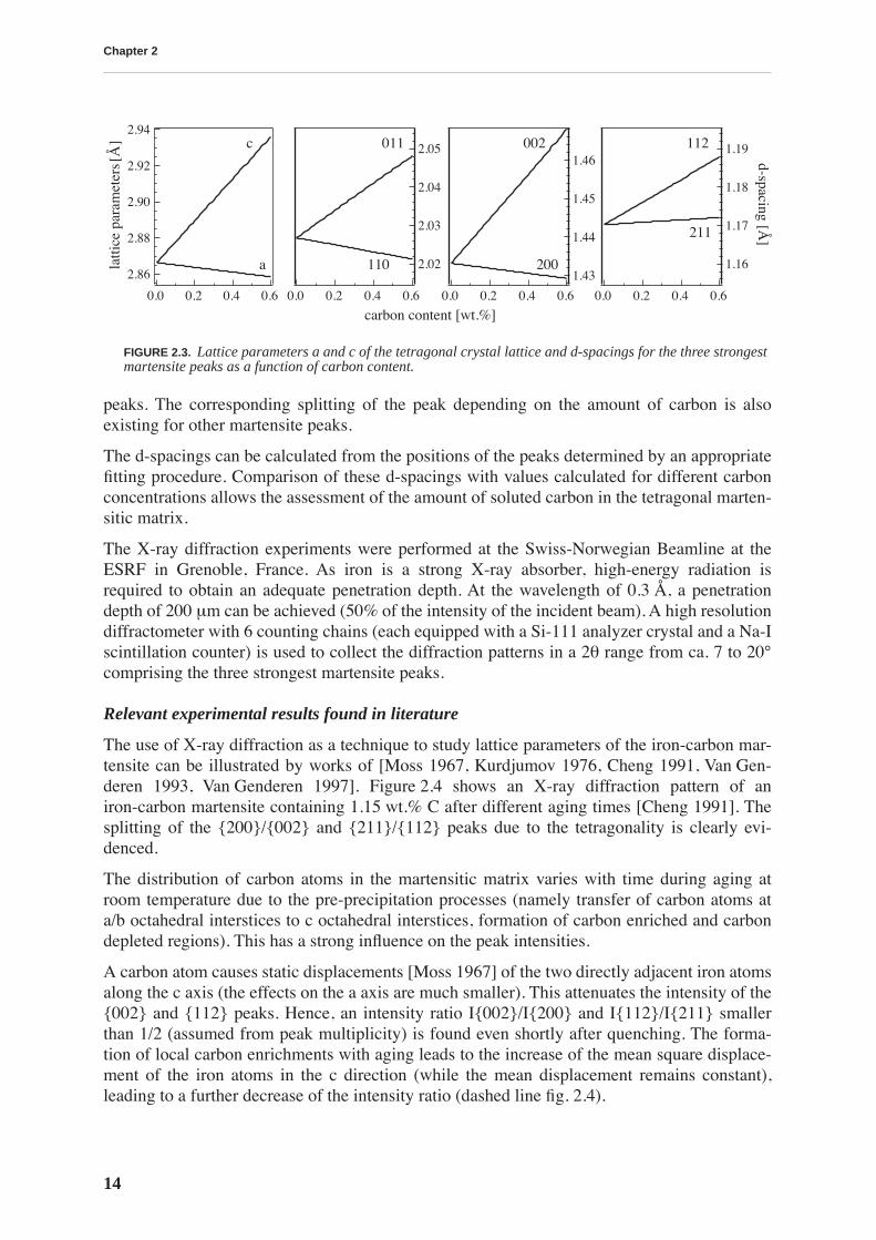
-spacings calcu-lated for different carbon concentrations for the three strongest martensite peaks, are given infig. 2.3 according to eq. 1.2, eq. 1.3 and eq. 2.2.
Therefore, the equivalence of e.g. crystal planes {011}, {101} and {110} in the bcc structure,which contribute to one X-ray diffraction peak, determined by the common d-spacing of2.027 Å, is not present in the tetragonal martensite. Due to the slight shortening of parameter
a
and the larger lengthening of the parameter
c
with the addition of carbon, a slight decrease ofthe d-spacing is expected for the {110} planes, and an increase of the d-spacing for the planes{011} and {101}. The two types of planes will consequently contribute to two diffraction
FIGURE 2.2.
a) Scheme of the AFM setup based on the laser beam deflection method for detecting normal (b)and lateral (c) deformation of the AFM cantilever (taken from [Kis 2003]).
scanner
cantileverAFM tip
laser
photodiode
A B
C D
feedback
(a) (b)
(c)
nλ 2d θsin=
dhklac
h2 k2+( )c2 l2a2
+-----------------------------------------------=
Chapter 2
14
peaks. The corresponding splitting of the peak depending on the amount of carbon is alsoexisting for other martensite peaks.
The d-spacings can be calculated from the positions of the peaks determined by an appropriatefitting procedure. Comparison of these d-spacings with values calculated for different carbonconcentrations allows the assessment of the amount of soluted carbon in the tetragonal marten-sitic matrix.
The X-ray diffraction experiments were performed at the Swiss-Norwegian Beamline at theESRF in Grenoble, France. As iron is a strong X-ray absorber, high-energy radiation isrequired to obtain an adequate penetration depth. At the wavelength of 0.3 Å, a penetrationdepth of 200
µ
m can be achieved (50% of the intensity of the incident beam). A high resolutiondiffractometer with 6 counting chains (each equipped with a Si-111 analyzer crystal and a Na-Iscintillation counter) is used to collect the diffraction patterns in a 2
θ
range from ca. 7 to 20°comprising the three strongest martensite peaks.
Relevant experimental results found in literature
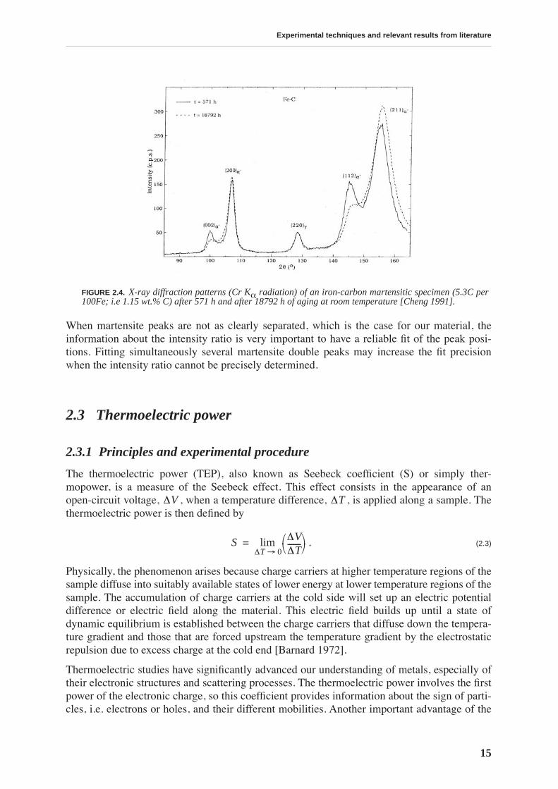
The use of X-ray diffraction as a technique to study lattice parameters of the iron-carbon mar-tensite can be illustrated by works of [Moss 1967, Kurdjumov 1976, Cheng 1991, Van Gen-deren 1993, Van Genderen 1997]. Figure 2.4 shows an X-ray diffraction pattern of aniron-carbon martensite containing 1.15 wt.% C after different aging times [Cheng 1991]. Thesplitting of the {200}/{002} and {211}/{112} peaks due to the tetragonality is clearly evi-denced.
The distribution of carbon atoms in the martensitic matrix varies with time during aging atroom temperature due to the pre-precipitation processes (namely transfer of carbon atoms ata/b octahedral interstices to c octahedral interstices, formation of carbon enriched and carbondepleted regions). This has a strong influence on the peak intensities.
A carbon atom causes static displacements [Moss 1967] of the two directly adjacent iron atomsalong the c axis (the effects on the a axis are much smaller). This attenuates the intensity of the{002} and {112} peaks. Hence, an intensity ratio I{002}/I{200} and I{112}/I{211} smallerthan 1/2 (assumed from peak multiplicity) is found even shortly after quenching. The forma-tion of local carbon enrichments with aging leads to the increase of the mean square displace-ment of the iron atoms in the c direction (while the mean displacement remains constant),leading to a further decrease of the intensity ratio (dashed line fig. 2.4).
FIGURE 2.3.
Lattice parameters a and c of the tetragonal crystal lattice and d-spacings for the three strongestmartensite peaks as a function of carbon content.
1.19
1.18
1.17
1.16
d-spacing [Å]
0.60.40.20.0
1.46
1.45
1.44
1.43
0.60.40.20.0
2.94
2.92
2.90
2.88
2.86
latt
ice
para
met
ers [
Å]
0.60.40.20.0
2.05
2.04
2.03
2.02
0.60.40.20.0
carbon content [wt.%]
c
211
112
200
002
110
011
a
Experimental techniques and relevant results from literature
15
When martensite peaks are not as clearly separated, which is the case for our material, theinformation about the intensity ratio is very important to have a reliable fit of the peak posi-tions. Fitting simultaneously several martensite double peaks may increase the fit precisionwhen the intensity ratio cannot be precisely determined.
2.3 Thermoelectric power
2.3.1 Principles and experimental procedure
The thermoelectric power (TEP), also known as Seebeck coefficient (S) or simply ther-mopower, is a measure of the Seebeck effect. This effect consists in the appearance of anopen-circuit voltage, , when a temperature difference, , is applied along a sample. Thethermoelectric power is then defined by
.
(2.3)
Physically, the phenomenon arises because charge carriers at higher temperature regions of thesample diffuse into suitably available states of lower energy at lower temperature regions of thesample. The accumulation of charge carriers at the cold side will set up an electric potentialdifference or electric field along the material. This electric field builds up until a state ofdynamic equilibrium is established between the charge carriers that diffuse down the tempera-ture gradient and those that are forced upstream the temperature gradient by the electrostaticrepulsion due to excess charge at the cold end [Barnard 1972].
Thermoelectric studies have significantly advanced our understanding of metals, especially oftheir electronic structures and scattering processes. The thermoelectric power involves the firstpower of the electronic charge, so this coefficient provides information about the sign of parti-cles, i.e. electrons or holes, and their different mobilities. Another important advantage of the
FIGURE 2.4.
X-ray diffraction patterns (Cr K
α
radiation) of an iron-carbon martensitic specimen (5.3C per100Fe; i.e 1.15 wt.% C) after 571 h and after 18792 h of aging at room temperature [Cheng 1991].
∆V ∆T
S ∆V∆T-------⎝ ⎠⎛ ⎞
∆T 0→lim=
Chapter 2
16
measurements of TEP over measurements of electric resistivity is that they are independent ofthe sample geometry.
The thermoelectric phenomena in metals are related to fundamental features of electronicenergy levels and to interactions of conduction electrons with their environment. A metal, evenan ideal pure single crystal, is a complex many-body system. The theory of transport propertiesis even more complicated for transition metals, which have overlapping s- and d-bands at theFermi surface, responsible for many interesting properties: the TEP of transition metals isroughly an order of magnitude greater than that of “simple” metals. Additionally, magneticeffects have to be taken into account when the TEP of iron is considered. A detailed descriptionof thermoelectric phenomena in metals can be found, for example, in [MacDonald 1962, Bar-nard 1972] or [Blatt 1976]. Some basic notions of different contributions to the TEP in metalsare described below.
The contribution to thermoelectric power due to electron diffusion,
S
d
, can be described by theMott expression:
,
(2.4)
where
σ(
Ε
) is the electric conductivity in the metal for electrons of energy
E
,
k
is the Boltz-mann constant and
e
the electron charge. The derivative has to be evaluated at the Fermi energy
E
F
. This contribution to the TEP is associated with a system of electrons that interacts with arandom distribution of scattering centers in thermal equilibrium at the local temperature
T
.
In a real system, the effect of temperature gradient on the lattice has to be considered as well asthe effect of the gradient on electrons. The temperature gradient causes an energy flow fromthe hotter to the colder region of the material in the form of phonons. The streaming phononscan interact with electrons, producing a contribution to thermopower, especially important atlow temperatures. This phenomenon is called the phonon-drag and the contribution to TEP,
S
g
,can be approximately described by:
,
(2.5)
where
C
g
is the specific heat of the lattice (subscript
g
is coming from the German word “Git-ter” for lattice),
N
is the density of conduction electrons and
α
, which lies between 0 and 1, is ameasure of the probability of a phonon colliding with an electron.
The effect analog to phonon-drag, when lattice vibration waves, phonons, are replaced by spinwaves, magnons, can appear in ferroelectric metals. It is described with an expression analogto eq. 2.5, only in the expression for
S
m
,
C
g
has to be replaced by
C
m
, the magnon specific heat.
Thermopower measurements were performed on an apparatus made at INSA, Lyon [Borrelly1985], schematized in fig. 2.5. The ends of the sample are fixed by teflon screws to two copperblocks marked
A
and B, the temperatures of which are kept constant by the regulatory system.The distance between the blocks can be regulated so that the length l ranges between 4 and11 cm. The block A is maintained at temperature T using a cooling Peltier module M, while theblock B is held at temperature T+∆T by means of a heating resistor R. Both blocks are con-nected with copper wires W to the isothermal switch I. This way the sample forms a differentialthermocouple with copper as a reference material and the ratio of the electrical potential differ-ence ∆V developed because of the temperature difference ∆T gives the relative thermopower∆S:
Sdπ2k2T3 e
--------------– ∂ σ E( )ln∂E
---------------------⎝ ⎠⎛ ⎞
E EF==
SgCg
3Ne----------α=
Experimental techniques and relevant results from literature
17
. (2.6)
The expression 2.6 is valid under two conditions. First, that ∆T is sufficiently small, so thatS(T) between T and T+∆T can be considered as linear, and second, that the heat flux throughthe sample can be considered as negligible. The temperature difference ∆T is measured by adifferential thermocouple placed just under the contact points of the sample. The ratio betweenthe amplified values of ∆V and ∆T is obtained using a voltage divider, and the value acquired isdisplayed (fig. 2.6).
The temperature T is set to 15.0±0.1 ºC and ∆T to 10.0±0.1 ºC. The absolute thermopower ofcopper at 20 ºC, SCu, is 1.80±0.01 µV/K [Blatt 1976], and this value should be added to themeasured one to get the absolute thermopower of the sample. As the nominal precision of themeasured value, 0.3%, with the resolution 0.002 µV/K, is better than the precision of the abso-lute thermopower of copper, it is the relative thermopower that is presented in the followingchapters.
2.3.2 Relevant experimental results found in literature
Thermopower measurements are found to be a very sensitive probe for the material microstruc-ture. The applications are broad, from verifying the purity of metals (detecting elements insolid solution), through the study of martensitic and order-disorder transformations, precipita-tion processes, to plastic deformation effects (work hardening) [Borrelly 1979].
The TEP of iron exhibits a very large peak near 200 K (fig. 2.7), the effect of which is still verystrong at room temperature. Blatt et al. [Blatt 1967] suggested that the peak arises out of mag-non drag because phonon-drag peaks at temperatures as high as 200 K are unusual and becausecold working produced a barely perceptible difference in the thermopower-temperature rela-tion. However, other mechanisms, like spin-orbit scattering, electron-electron scattering oreven phonon drag are not completely excluded [Blatt 1976].
The effects of cold work as well as those of nitrogen and carbon on the TEP of iron were stud-ied by [Borrelly 1985] and [Benkirat 1988]. Both dislocations and interstitials are found todecrease the TEP measured at room temperature. The decrease of TEP with cold rolling isfound to be a linear function of the thickness reduction (fig. 2.8, TEP is measured relative to areference material with Sref = 13.2 µV/K). The sensitivity of TEP to the concentration of car-
FIGURE 2.5. Schematic representation of the installation for TEP measurements.
FIGURE 2.6. Installation for TEP measurements.
∆S Ssample= SCu– ∆V∆T-------=
divider
display
T T + ∆T
IT0
A B
M
sample
R
∆VW
W
l
Chapter 2
18
bon is used to study the kinetics for isothermal tempering (fig. 2.9, TEP is measured relative toa reference material with Sref = 13.2 µV/K). TEP stabilization levels P0, P1, and P2 are relatedto the residual equilibrium concentration of carbon in the presence of different carbides. Noeffect on the TEP is attributed to carbides. A linear dependence of thermoelectric power on car-bon concentration is proposed for extra-mild steels based on a comparison of TEP with mea-surements of the Snoek peak in internal friction (the height of which is proportional to thecarbon concentration, see section 2.5) [Borrelly 1993]. This proportionality enables a quantita-tive evaluation of the interstitial content. The method proposed by [Borrelly 1993] includes the
FIGURE 2.7. Thermopower of iron and iron alloys: Fe-A, annealed iron; Fe-U, unannealed iron; N1,Fe-0.6 at.% Ni alloy; N2, Fe-1.45 at.% Ni; P1, Fe-1 at.% Pt; P2, Fe-2 at.% Pt [Blatt 1967].
FIGURE 2.8. TEP of pure iron at 20 ºCas a function of the relative variation ofthickness during cold rolling [Borrelly1985].
FIGURE 2.9. Evolution of room temperature TEP as a function ofaging time at various temperatures for a quenchedFe-0.018 wt.% C alloy. Stabilization levels P0, P1, and P2 arerelated to the residual equilibrium concentration of carbon in thepresence of carbides [Benkirat 1988].
Experimental techniques and relevant results from literature
19
measurement of the TEP before and after precipitation of carbon in the region between 100 and250 ºC. An alternative, rather sophisticated method is proposed by [Lavaire 2004]. It is basedon the segregation of carbon to dislocations created by cold rolling. In fact, it was establishedthat the effect of interstitial atoms in solid solution disappears when these atoms are segregatedto dislocations.
2.4 Mechanical tests
The aim of this thesis is to relate the mechanical properties with the microstructure issued by aparticular heat treatment. Two methods are chosen for measuring mechanical properties: com-pression tests and nanoindentation. The compression test is a relatively simple and fast way ofprobing material strength and elastic limits. The advantage of using nanoindentation is the pos-sibility of testing mechanical properties not only for the bulk material, but also for the differentregions of the file profile.
2.4.1 Compression
Compression tests were performed at room temperature in a Schenk RMC 100 testingmachine, operating in inverse compression (see fig. 2.10) and supporting loads up to 25 kN atroom temperature. The TZM pistons are separated from the sample by two WC-Co platesinsuring a protection of the piston surface from a possible formation of indents. The appliedforce is measured by a load cell connected with the movable piston. The displacement is mea-sured by two extensometers.
The stress σ exerted on the sample is calculated from the applied force F taking into accountthe changes of the sample cross-section (under constant volume approximation) according to:
(2.7)
FIGURE 2.10. Scheme of the installation for compression tests. The sample is compressed between two TZMpistons whose positions are detected by extensometers. WC-Co plates protect the piston surface fromformation of indents.
extensometers
WC-Co plates
sample
load cell
fixedpiston
movablepiston
σ FS0-----
ll0----⋅=
Chapter 2
20
where S0 and l0 are initial sample cross-section and length, respectively, and l its length underload. The strain is calculated from the measured variation of the sample length as following:
(2.8)
Because WC-Co plates and TZM pistons also deform elastically during compression (howeverlittle) the slope of the elastic part of the compression curve gives the apparent Young’s modulusEapp, which is lower than the real Young’s modulus of the sample E. Supposing that a part ofthe installation deforms in series with the sample, the apparent modulus is given by:
(2.9)
where Em is an installation contribution depending on the sample size.
The stress-strain curves give also some information about the yield stress and the compressionstrength. The yield stress is defined in connection with the plastic strain and is established byan offset method. It is common to define as engineering yield stress the stress that would causea permanent deformation of 0.2%. The ideal elastic stress relaxation line is drawn parallel tothe elastic portion of the stress-strain curve upon loading, but offset from it by 0.2%. The stressread at the intersection of this line with the stress-strain curve is the yield stress. This proce-dure does not take into account anelastic effects. The compression strength (also called the ulti-mate strength) is defined as the maximum stress a material is capable to attain.
Samples for compression tests are spark-cut from the bulk of the file to the dimensions mm3 taking special care to make the compressed surfaces parallel. Experi-
ments are performed at constant piston speed, set to 40 µm/min, giving a starting strain rate of0.0146 s-1.
2.4.2 Nanoindentation
Hardness is generally defined as the resistance of a material to plastic deformation, usually byindentation, although the term may also refer to resistance to scratching, abrasion or cutting. Itis clear that, lacking a more precise definition, hardness can be expressed quantitatively onlywithin a defined measurement procedure. Several relatively simple hardness test methodsapplying different indent geometries are widely used in industry (Rockwell, Brinell, Vickershardness etc.). A big advance in hardness measurement came with the development of instru-ments that continuously measure force and displacement as an indentation is made. Moreover,it is possible to test the mechanical properties at submicron scale. The analysis of the load-dis-placement data is made according to the method proposed by Oliver and Pharr [Oliver 1992].
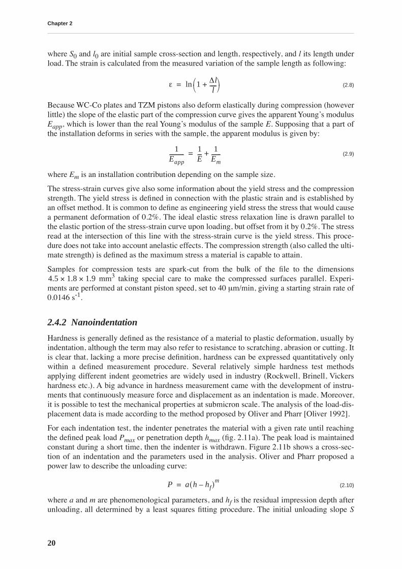
For each indentation test, the indenter penetrates the material with a given rate until reachingthe defined peak load Pmax or penetration depth hmax (fig. 2.11a). The peak load is maintainedconstant during a short time, then the indenter is withdrawn. Figure 2.11b shows a cross-sec-tion of an indentation and the parameters used in the analysis. Oliver and Pharr proposed apower law to describe the unloading curve:
(2.10)
where a and m are phenomenological parameters, and hf is the residual impression depth afterunloading, all determined by a least squares fitting procedure. The initial unloading slope S
ε 1 ∆ll
-----+⎝ ⎠⎛ ⎞ln=
1Eapp-----------
1E---
1Em-------+=
4.5 1.8 1.9××
P a h hf–( )m=
Experimental techniques and relevant results from literature
21
(contact stiffness) is then found by analytically differentiating this expression and evaluatingthe derivative at the peak load and displacement:
. (2.11)
The vertical distance along which the contact is made (the contact depth) hc can then be calcu-lated according to:
(2.12)
where is a constant depending on the indenter geometry.
The mechanical properties of the sample that can be obtained from one complete cycle of load-ing and unloading are hardness and elastic modulus. Hardness is defined as:
(2.13)
where Pmax is the peak indentation load and A is the projected area of the elastic contact, calcu-lated as , depending on the indenter geometry. Taking into account the influences ofa non-rigid indenter, one can define the reduced elastic modulus Er through the equation
, (2.14)
where E and ν are Young’s modulus and Poisson’s ratio for the sample, and Ei and νi are thesame parameters for the indenter (for diamond the values are Ei = 1141 GPa and νi = 0.07).The reduced modulus defined above can be obtained from the experimentally measured stiff-ness S for unloading according to:
a) b)
FIGURE 2.11. a) A schematic representation of load versus indenter displacement for an indentationexperiment. The quantities shown are the maximal indentation load Pmax and the indenter displacementhmax, the final depth of the contact impression after unloading hf and the initial unloading stiffness S. b) Aschematic representation of elasto-plastic deformation induced by the indenter. At any time during loading,the total displacement h is a sum of hs, the displacement of the surface at the perimeter of the contact, andthe distance along which the contact is made (the contact depth), hc.
Pmax
h max
h f
Sloading
unloading
Displacement, h
Load
, P
initial surface
surface profileunder load
h f
h ch s
h
indenter
surface profileafter load removal
S dPdh-------
h hmax=
ma hmax hf–( )m 1–= =
hc hmax κPmax
S-----------–=
κ
HPmax
A-----------=
A f hc( )=
1Er-----
1 ν2–( )E
-------------------1 νi
2–( )
Ei---------------------+=
Chapter 2
22
(2.15)
where is a correction factor arising from the fact that the indenter shape does not have a rota-tional symmetry.
Nanoindentation experiments were performed on a Nano Indenter XP system with a Berkovichtype diamond tip (triangular based pyramid, giving = 0,75 and = 1.034), using the contin-uous stiffness method. This technique superimposes an oscillating load of small amplitude andhigh frequency to the nominal indenting load allowing continuous measurements of elasticmodulus and hardness as the indenter penetrates the material. A more detailed description ofthe installation and dynamic measurements is given in [Azcoïtia 2002] and the original Oliverand Pharr paper [Oliver 1992].
As already pointed out, the aim of the nanoindentation tests was to probe the mechanical prop-erties not only in the bulk, as with compression tests, but more locally. For that reason, across-section of the file is obtained perpendicularly to the teeth (on one file side) to allow themeasurements on the teeth as well (otherwise not meaningful because of the deformation ofthe tooth). 5 mm thick samples extracted from the files were mechanically polished as forAFM, using colloidal silica solution of 0.1 µm particle size.
2.5 Mechanical spectroscopy
The concept of anelastic relaxation that has been introduced in 1948 by Zener [Zener 1948],and related topics such as internal friction and mechanical spectroscopy, are described in detailin the classic book by Nowick and Berry [Nowick 1972a] and more recently in the textbookresulting from the summer school “Mechanical spectroscopy Q-1 2001” [Schaller 2001].
2.5.1 Phenomenology and definitions
Under the condition that the stress applied on a material is sufficiently low (lower than the elas-tic limit), the material will not deform plastically. In that case, the response of the material willbe a deformation that can be completely recovered upon release of the applied stress, com-posed of an elastic and an anelastic part. The elastic deformation, in addition to the completerecoverability, fulfills the requirement of being linearly proportional to the applied stress andbeing instantaneous. The anelastic part, usually much lower in magnitude, differs from theelastic one merely in the way that the equilibrium response is achieved after sufficient time.The anelastic response is related with the motion of defects in the material and results in a dis-sipation of energy.
The internal friction (IF), also called the mechanical loss, is a measure of this energy dissipa-tion in the case of an applied cyclic stress. It is defined as:
(2.16)
where ∆W is the energy dissipated and W the energy stored during one cycle. The internal fric-tion is directly related to the number and kind of mobile microstructural units inside the solid,as well as to the characteristic motion that they undergo. Therefore, the measurement of inter-nal friction can be used to obtain information about the microstructure of the material in anon-destructive way. Mechanical spectroscopy is a spectroscopic technique in which a
Er1β---
π2
-------S
A-------⋅ ⋅=
β
κ β
IF 12π------
∆WW
---------=
Experimental techniques and relevant results from literature
23
mechanical oscillating stress of frequency ω interacts with the solid. The response of the solidinvolves the absorption of mechanical energy that we measure as a function of frequency, giv-ing an internal friction spectrum.
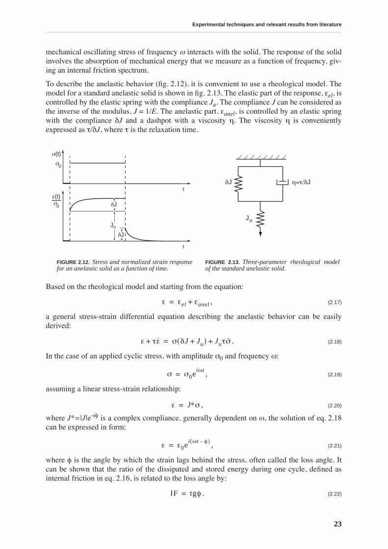
To describe the anelastic behavior (fig. 2.12), it is convenient to use a rheological model. Themodel for a standard anelastic solid is shown in fig. 2.13. The elastic part of the response, εel, iscontrolled by the elastic spring with the compliance Ju. The compliance J can be considered asthe inverse of the modulus, J = 1/E. The anelastic part, εanel, is controlled by an elastic springwith the compliance δJ and a dashpot with a viscosity η. The viscosity η is convenientlyexpressed as τ/δJ, where τ is the relaxation time.
Based on the rheological model and starting from the equation:
, (2.17)
a general stress-strain differential equation describing the anelastic behavior can be easilyderived:
. (2.18)
In the case of an applied cyclic stress, with amplitude σ0 and frequency ω:
, (2.19)
assuming a linear stress-strain relationship:
, (2.20)
where J*=|J|e-iφ is a complex compliance, generally dependent on ω, the solution of eq. 2.18can be expressed in form:
, (2.21)
where φ is the angle by which the strain lags behind the stress, often called the loss angle. Itcan be shown that the ratio of the dissipated and stored energy during one cycle, defined asinternal friction in eq. 2.16, is related to the loss angle by:
. (2.22)
FIGURE 2.12. Stress and normalized strain responsefor an anelastic solid as a function of time.
FIGURE 2.13. Three-parameter rheological modelof the standard anelastic solid.
σ(t)
t
t
δJ
δJ
σ0
Ju
σ0
ε(t)
η=τ/δJ
Ju
δJ
ε εel εanel+=
ε τε̇+ σ δJ Ju+( ) Juτσ̇+=
σ σ0eiωt=
ε J∗σ=
ε ε0ei ωt φ–( )=
IF tgφ=
Chapter 2
24
Another useful quantity is the relative variation of the dynamic compliance (or correspond-ingly, the so called modulus defect):
(2.23)
From equations 2.18 - 2.23, and in the case of δJ<<Ju, it follows that:
(2.24)
. (2.25)
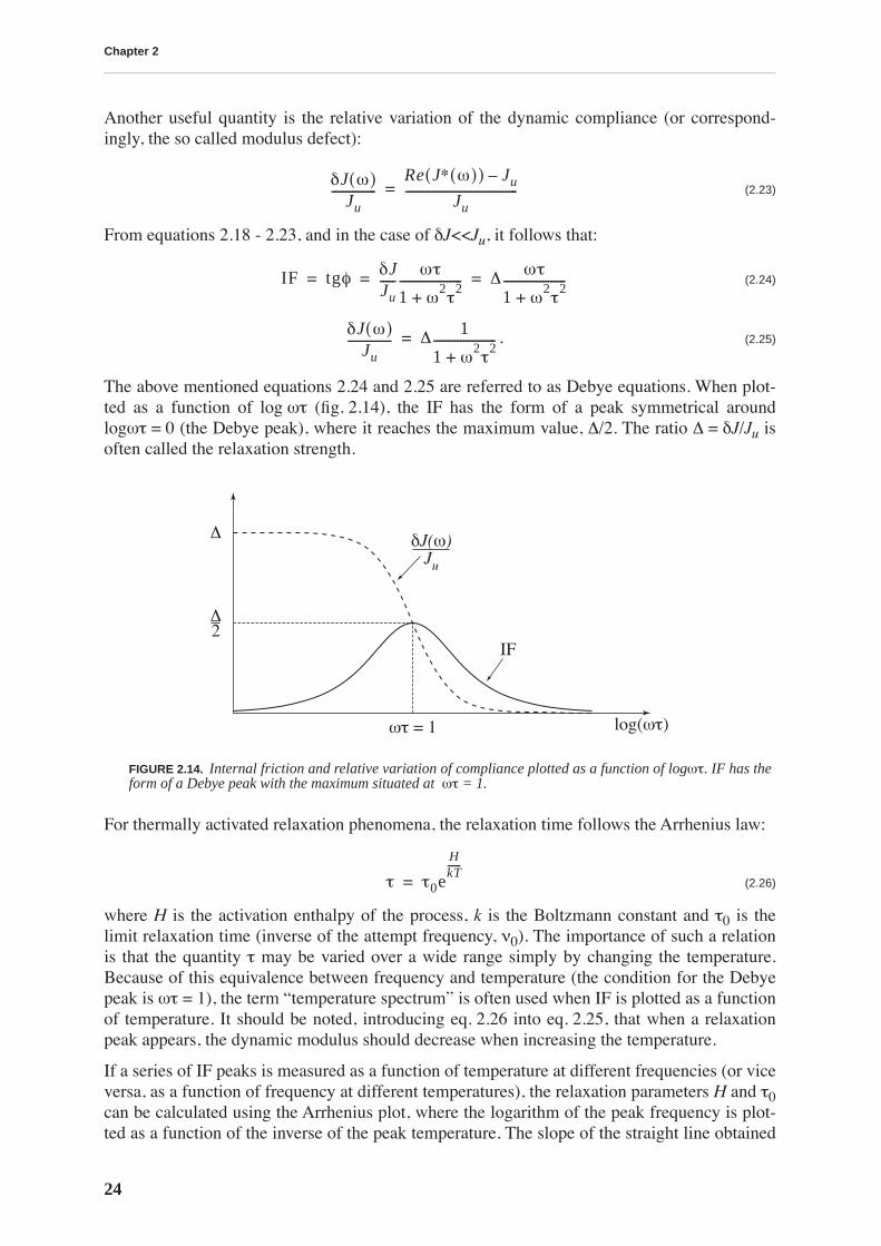
The above mentioned equations 2.24 and 2.25 are referred to as Debye equations. When plot-ted as a function of log ωτ (fig. 2.14), the IF has the form of a peak symmetrical aroundlogωτ = 0 (the Debye peak), where it reaches the maximum value, ∆/2. The ratio ∆ = δJ/Ju isoften called the relaxation strength.
For thermally activated relaxation phenomena, the relaxation time follows the Arrhenius law:
(2.26)
where H is the activation enthalpy of the process, k is the Boltzmann constant and τ0 is thelimit relaxation time (inverse of the attempt frequency, ν0). The importance of such a relationis that the quantity τ may be varied over a wide range simply by changing the temperature.Because of this equivalence between frequency and temperature (the condition for the Debyepeak is ωτ = 1), the term “temperature spectrum” is often used when IF is plotted as a functionof temperature. It should be noted, introducing eq. 2.26 into eq. 2.25, that when a relaxationpeak appears, the dynamic modulus should decrease when increasing the temperature.
If a series of IF peaks is measured as a function of temperature at different frequencies (or viceversa, as a function of frequency at different temperatures), the relaxation parameters H and τ0can be calculated using the Arrhenius plot, where the logarithm of the peak frequency is plot-ted as a function of the inverse of the peak temperature. The slope of the straight line obtained
FIGURE 2.14. Internal friction and relative variation of compliance plotted as a function of logωτ. IF has theform of a Debye peak with the maximum situated at ωτ = 1.
δJ ω( )Ju
---------------Re J∗ ω( )( ) Ju–
Ju--------------------------------------=
IF tgφ δJJu-----
ωτ
1 ω2τ2+
--------------------- ∆ ωτ
1 ω2τ2+
---------------------= = =
δJ ω( )Ju
--------------- ∆ 1
1 ω2τ2+
---------------------=
log(ωτ)ωτ = 1
∆2
∆
IF
Ju
δJ(ω)
τ τ0e
HkT------
=
Experimental techniques and relevant results from literature
25
gives H, and the intercept with the y-axis gives τ0. Analogously, knowing one temperature andfrequency of the peak together with its activation energy, enables the prediction of the peaktemperature for a given frequency (or frequency for a given temperature) according to theexpression:
(2.27)
that is easily derived combining eq. 2.26 and the peak condition ωτ = 1. There are many caseswhere there is no single relaxation time associated with a physical process. It is often necessaryto define a distribution of relaxation times. In that case, the internal friction can be described bythe expression:
, . (2.28)
where α is a broadening factor [Fuoss 1941].
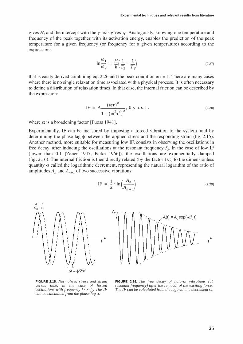
Experimentally, IF can be measured by imposing a forced vibration to the system, and bydetermining the phase lag φ between the applied stress and the responding strain (fig. 2.15).Another method, more suitable for measuring low IF, consists in observing the oscillations infree decay, after inducing the oscillations at the resonant frequency f0. In the case of low IF(lower than 0.1 [Zener 1947, Parke 1966]), the oscillations are exponentially damped(fig. 2.16). The internal friction is then directly related (by the factor 1/π) to the dimensionlessquantity α called the logarithmic decrement, representing the natural logarithm of the ratio ofamplitudes An and An+1 of two successive vibrations:
(2.29)
FIGURE 2.15. Normalized stress and strainversus time, in the case of forcedoscillations with frequency f << f0. The IFcan be calculated from the phase lag φ.
FIGURE 2.16. The free decay of natural vibrations (atresonant frequency) after the removal of the exciting force.The IF can be calculated from the logarithmic decrement α.
ω1
ω2------ln H
k----
1T2-----
1T1-----–⎝ ⎠
⎛ ⎞=
IF ∆ ωτ( )α
1 ω2τ2( )α
+-----------------------------= 0 α 1≤<
IF 1π---
An
An 1+-------------⎝ ⎠⎛ ⎞ln⋅=
t
σσ0
εε0
∆t = φ/2πf
AA(t) = A exp(-αf t)
0
0 0
t

Chapter 2
26
2.5.2 Experimental installations
As the relaxation processes in the material depend both on temperature and frequency, themeasurements of internal friction are performed on different types of installations. Thefree-free vibrating reed installation is used to study the IF at high frequencies (1-3 kHz) andthe inverted torsion pendulum to study the IF at low frequencies (0.5 - 3 Hz). The temperaturerange is 80-800 K for high and 90-700 K for the low frequency installation. The standard heat-ing rate used is 1 K/min, if not otherwise mentioned.
Free-free vibrating reed installation
The principle of measuring internal friction in the free-free vibrating reed installation has beendescribed in detail by [Vittoz 1963]. A rectangular sample suspended between two pairs of thinwires, placed at nodal lines of the first flexural vibration mode, is excited to oscillate at its res-onant frequency by means of an excitation-detection electrode (fig. 2.17). The electrode, posi-tioned above the center of the sample, forms with it a capacitor.
When a voltage of the form
(2.30)
is applied to the electrode, an electrostatic force F acts on the sample:
, (2.31)
where A is the surface of the electrode, d the interelectrode gap and ε0 the vacuum permittivity.Under the condition that U0>U1, the electronics part of the installation filters the frequency ofthe excitation in order to be the resonant frequency of the sample. A resonant frequency
for the first flexural vibration mode is found to be [Vittoz 1963]:
(2.32)
where h is the thickness, b the width and l the length of the sample, E its Young’s modulus andρ and m its density and mass, respectively. The distance x of the nodal line from the end of thesample is in this case 0.2241l. The detection of the oscillations is made by including the
FIGURE 2.17. Scheme of the free-free vibrating reed installation. A rectangular sample suspended betweentwo pairs of wires placed at the nodal lines of the first flexural vibration mode is excited to oscillate at itsresonant frequency by means of an electrode.
b
l
x
h
U U0 U1 ωt( )sin+=
Fε0A
d2--------- U0U1 ωt( ) 14---U1
2 2ωt( ) 12--- U0
2 12---U1
2+⎝ ⎠
⎛ ⎞+cos–sin=
f ω2π------=
f 9π
16 3-------------
h
l2----Eρ--- 9π
16 3-------------
h3 2⁄ b1 2⁄
l3 2⁄---------------------Em----= =
Experimental techniques and relevant results from literature
27
sample-electrode capacitor into an RCL circuit oscillating at high frequency (3.6 MHz). Thevariation of the electric capacitance due to the changing distance between the sample and theelectrode causes a frequency modulation of the high frequency carrier signal (radio principle).A servo-motor holds the electrode gap constant so that no variation occurs in the carrier fre-quency and the vibrating amplitude as a result of the thermal dilatation of the electrode-samplesystem. A more detailed description of the installation can be found in [Fornerod 1968] and[Isoré 1973].
After stopping the excitation, the number n of oscillations in free decay between two fixedamplitudes Ai and Ai+n is recorded. Internal friction is then calculated according to:
(2.33)
The chosen length of the samples is 40 mm in order to have the nodal points of the first flexuraloscillation mode at the distance fixed in the setup, the width of the sample is 4 mm and thethickness is varied between 0.3 and 1 mm. The maximum strain amplitude varies from 10-7 to10-6.
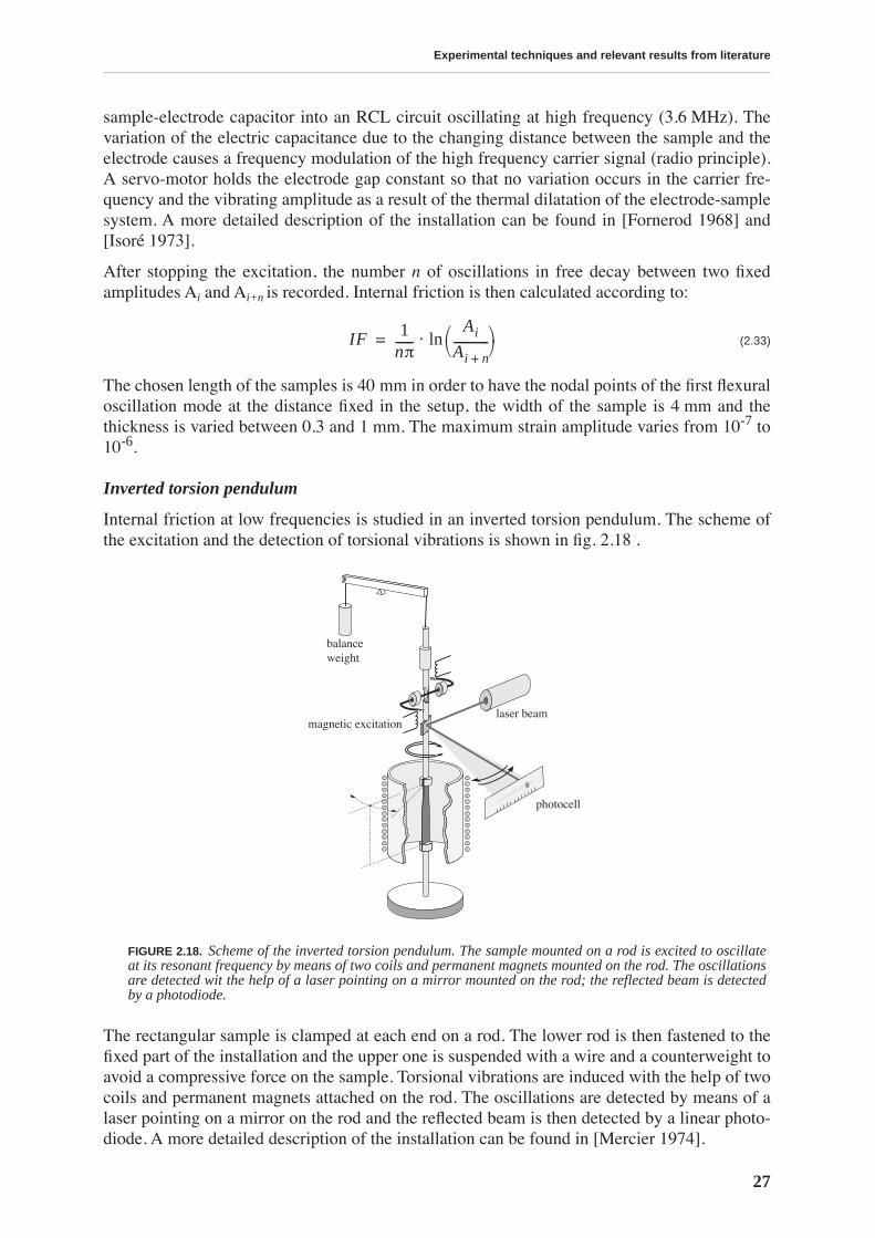
Inverted torsion pendulum
Internal friction at low frequencies is studied in an inverted torsion pendulum. The scheme ofthe excitation and the detection of torsional vibrations is shown in fig. 2.18 .
The rectangular sample is clamped at each end on a rod. The lower rod is then fastened to thefixed part of the installation and the upper one is suspended with a wire and a counterweight toavoid a compressive force on the sample. Torsional vibrations are induced with the help of twocoils and permanent magnets attached on the rod. The oscillations are detected by means of alaser pointing on a mirror on the rod and the reflected beam is then detected by a linear photo-diode. A more detailed description of the installation can be found in [Mercier 1974].
FIGURE 2.18. Scheme of the inverted torsion pendulum. The sample mounted on a rod is excited to oscillateat its resonant frequency by means of two coils and permanent magnets mounted on the rod. The oscillationsare detected wit the help of a laser pointing on a mirror mounted on the rod; the reflected beam is detectedby a photodiode.
IF 1nπ------
Ai
Ai n+------------⎝ ⎠⎛ ⎞ln⋅=
laser beam
photocell
magnetic excitation
balanceweight
Chapter 2
28
Again, as in the case of torsional vibrations, the frequency of oscillations is the resonant fre-quency, which depends on the sample parameters:
(2.34)
where G is the shear modulus, I the moment of inertia of the rod-sample system, b and h arethe previously described sample dimensions, while l is in this case the free length of the sample(between clamps). A numerical coefficient β is necessary to describe the torsional rigidity of arectangular bar and it is dependent of the b/h ratio [Timoshenko 1963]. Typical sample dimen-sions (between the clamps) are mm3, resulting in a value of β = 0.319. The maxi-mum strain amplitude is 10-5. The internal friction is measured as in the case of the vibratingreed setup, observing the free decay of the oscillations.
Some measurements are also made in a forced inverted torsion pendulum where the sample isforced to oscillate at a chosen frequency well below the resonant one. The scheme of the pen-dulum is similar to the one presented in fig. 2.18, but the internal friction is measured from thephase lag (fig. 2.15, eq. 2.24) between excitation and the mechanical response of the sample.The advantage of using a forced pendulum is the possibility to vary the oscillation frequency ina broad range on a single sample. The measurements in free decay, on the other hand, give abetter possibility to measure very low levels of internal friction.
2.5.3 Relevant experimental results found in literature
Various relaxation mechanisms are found to contribute to the internal friction in bcc metals,involving point defects, dislocations, or both when interacting. They are briefly described inthe following paragraphs. In addition to relaxation mechanisms, internal friction is also influ-enced by phase transformations resulting in features which are not thermally activated. One ofthese phenomena is the martensitic transformation. The isothermal martensitic transformationhas been studied by internal friction in Fe-Ni and Fe-Ni-C alloys [Rodriguez 1984]. As themartensitic transformation in our material only occurs upon quenching, and is completely fin-ished at room temperature, these results are of little relevance for this work. The reverse trans-formation upon heating is not sudden. The diffusion of carbon and the formation of carbidesdepletes the martensitic matrix of carbon in solid solution and martensite gradually decom-poses into ferrite.
One of the most famous point defect relaxation mechanisms is certainly the one causing the socalled Snoek IF peak [Nowick 1972b, Weller 2001]. The term Snoek relaxation refers to theanelastic relaxation in bcc metals produced by interstitial solutes in the process ofstrain-induced ordering. It was first observed by Snoek [Snoek 1939] in α-iron loaded withnitrogen and carbon, but it is now known that other bcc metals (e.g. Ta, Nb, Cr, V) exhibit arelaxation of the same type with different interstitials (H, O, in addition to C and N). The pre-requisite for an anelastic relaxation by point defects is the existence of several defect positions.An interstitial atom occupying the octahedral interstitial position in a bcc crystal lattice(fig. 1.1c) constitutes an elastic dipole of tetragonal symmetry, with the symmetry axis lyingalong the mayor axis of the octahedron. The tetragonal axis may lie along any of the cube axes.Therefore, in case of equilibrium without external stress, the octahedral sites may be dividedinto three groups of crystallographically equivalent sites. Under the effect of an applied stress,one orientation is preferred and the interstitials jump between neighboring octahedral sitescausing the reorientation of elastic dipoles. This relaxation process results in the formation ofan internal friction peak with an amplitude proportional to the concentration of interstitials in
f 12π------
βGbh3
lI-----------------=
10 4 0.3××
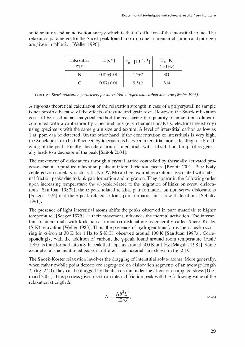
Experimental techniques and relevant results from literature
29
solid solution and an activation energy which is that of diffusion of the interstitial solute. Therelaxation parameters for the Snoek peak found in α-iron due to interstitial carbon and nitrogenare given in table 2.1 [Weller 1996].
A rigorous theoretical calculation of the relaxation strength in case of a polycrystalline sampleis not possible because of the effects of texture and grain size. However, the Snoek relaxationcan still be used as an analytical method for measuring the quantity of interstitial solutes ifcombined with a calibration by other methods (e.g. chemical analysis, electrical resistivity)using specimens with the same grain size and texture. A level of interstitial carbon as low as1 at. ppm can be detected. On the other hand, if the concentration of interstitials is very high,the Snoek peak can be influenced by interactions between interstitial atoms, leading to a broad-ening of the peak. Finally, the interaction of interstitials with substitutional impurities gener-ally leads to a decrease of the peak [Saitoh 2004].
The movement of dislocations through a crystal lattice controlled by thermally activated pro-cesses can also produce relaxation peaks in internal friction spectra [Benoit 2001]. Pure bodycentered cubic metals, such as Ta, Nb, W, Mo and Fe, exhibit relaxations associated with inter-nal friction peaks due to kink pair formation and migration. They appear in the following orderupon increasing temperature: the α'-peak related to the migration of kinks on screw disloca-tions [San Juan 1987b], the α-peak related to kink pair formation on non-screw dislocations[Seeger 1976] and the γ-peak related to kink pair formation on screw dislocations [Schultz1991].
The presence of light interstitial atoms shifts the peaks observed in pure materials to highertemperatures [Seeger 1979], as their movement influences the thermal activation. The interac-tion of interstitials with kink pairs formed on dislocations is generally called Snoek-Köster(S-K) relaxation [Weller 1983]. Thus, the presence of hydrogen transforms the α-peak occur-ring in α-iron at 30 K for 1 Hz to S-K(H) observed around 100 K [San Juan 1987a]. Corre-spondingly, with the addition of carbon, the γ-peak found around room temperature [Astié1980] is transformed into a S-K peak that appears around 500 K at 1 Hz [Magalas 1981]. Someexamples of the mentioned peaks in different bcc materials are shown in fig. 2.19.
The Snoek-Köster relaxation involves the dragging of interstitial solute atoms. More generally,when rather mobile point defects are segregated on dislocation segments of an average length
(fig. 2.20), they can be dragged by the dislocation under the effect of an applied stress [Gre-maud 2001]. This process gives rise to an internal friction peak with the following value of therelaxation strength ∆:
, (2.35)
TABLE 2.1 Snoek relaxation parameters for interstitial nitrogen and carbon in α-iron [Weller 1996].
interstitial type
H [eV] τ0-1 [1014s-1] Tm [K]
(f=1Hz)
N 0.82±0.01 4.2±2 300
C 0.87±0.01 5.3±2 314
L
∆ Λb2L2
12γJ----------------=
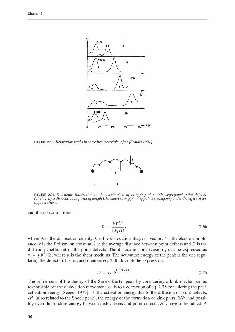
Chapter 2
30
and the relaxation time:
, (2.36)
where Λ is the dislocation density, b is the dislocation Burger’s vector, J is the elastic compli-ance, k is the Boltzmann constant, is the average distance between point defects and D is thediffusion coefficient of the point defects. The dislocation line tension γ can be expressed as
, where µ is the shear modulus. The activation energy of the peak is the one regu-lating the defect diffusion, and it enters eq. 2.36 through the expression:
(2.37)
The refinement of the theory of the Snoek-Köster peak by considering a kink mechanism asresponsible for the dislocation movement leads to a correction of eq. 2.36 considering the peakactivation energy [Seeger 1979]. To the activation energy due to the diffusion of point defects,HS, (also related to the Snoek peak), the energy of the formation of kink pairs, 2Hk, and possi-bly even the binding energy between dislocations and point defects, HB, have to be added. A
FIGURE 2.19. Relaxation peaks in some bcc materials, after [Schultz 1991].
FIGURE 2.20. Schematic illustration of the mechanism of dragging of mobile segregated point defects(circles) by a dislocation segment of length L between strong pinning points (hexagons) under the effect of anapplied stress.
l
L
f
τ kTL2
12γ lD---------------=
l
γ µb2 2⁄=
D D0eHS kT( )⁄=
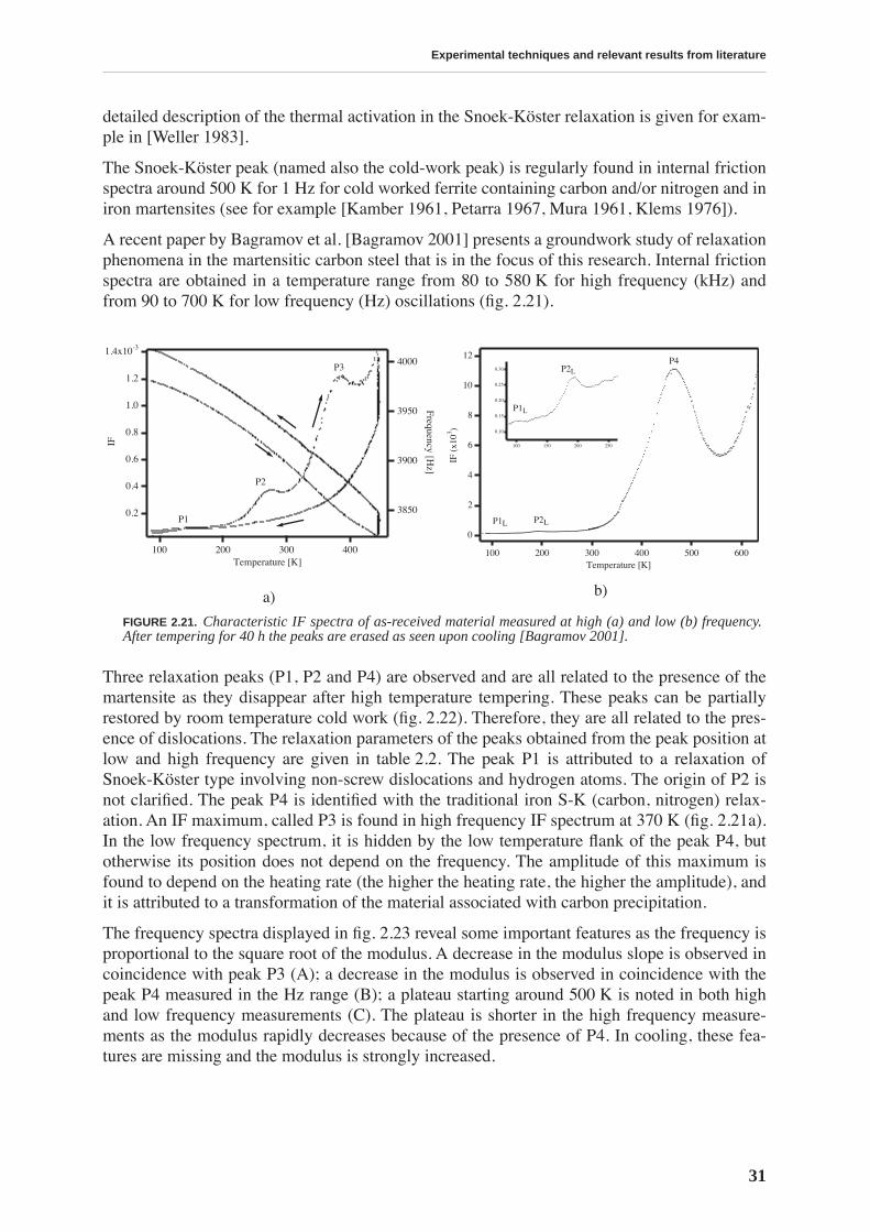
Experimental techniques and relevant results from literature
31
detailed description of the thermal activation in the Snoek-Köster relaxation is given for exam-ple in [Weller 1983].
The Snoek-Köster peak (named also the cold-work peak) is regularly found in internal frictionspectra around 500 K for 1 Hz for cold worked ferrite containing carbon and/or nitrogen and iniron martensites (see for example [Kamber 1961, Petarra 1967, Mura 1961, Klems 1976]).
A recent paper by Bagramov et al. [Bagramov 2001] presents a groundwork study of relaxationphenomena in the martensitic carbon steel that is in the focus of this research. Internal frictionspectra are obtained in a temperature range from 80 to 580 K for high frequency (kHz) andfrom 90 to 700 K for low frequency (Hz) oscillations (fig. 2.21).
Three relaxation peaks (P1, P2 and P4) are observed and are all related to the presence of themartensite as they disappear after high temperature tempering. These peaks can be partiallyrestored by room temperature cold work (fig. 2.22). Therefore, they are all related to the pres-ence of dislocations. The relaxation parameters of the peaks obtained from the peak position atlow and high frequency are given in table 2.2. The peak P1 is attributed to a relaxation ofSnoek-Köster type involving non-screw dislocations and hydrogen atoms. The origin of P2 isnot clarified. The peak P4 is identified with the traditional iron S-K (carbon, nitrogen) relax-ation. An IF maximum, called P3 is found in high frequency IF spectrum at 370 K (fig. 2.21a).In the low frequency spectrum, it is hidden by the low temperature flank of the peak P4, butotherwise its position does not depend on the frequency. The amplitude of this maximum isfound to depend on the heating rate (the higher the heating rate, the higher the amplitude), andit is attributed to a transformation of the material associated with carbon precipitation.
The frequency spectra displayed in fig. 2.23 reveal some important features as the frequency isproportional to the square root of the modulus. A decrease in the modulus slope is observed incoincidence with peak P3 (A); a decrease in the modulus is observed in coincidence with thepeak P4 measured in the Hz range (B); a plateau starting around 500 K is noted in both highand low frequency measurements (C). The plateau is shorter in the high frequency measure-ments as the modulus rapidly decreases because of the presence of P4. In cooling, these fea-tures are missing and the modulus is strongly increased.
a) b)
FIGURE 2.21. Characteristic IF spectra of as-received material measured at high (a) and low (b) frequency.After tempering for 40 h the peaks are erased as seen upon cooling [Bagramov 2001].
P1
P2
P3
1.4x10⁻³
1.2
1.0
0.8
0.6
0.4
0.2
IF
400300200100Temperature [K]
4000
3950
3900
3850
Frequency [Hz]
12
10
8
6
4
2
0
IF (
x103 )
600500400300200100Temperature [K]
P1L P2L
P4
P1L
P2L0.30
0.25
0.20
0.15
0.10
250200150100
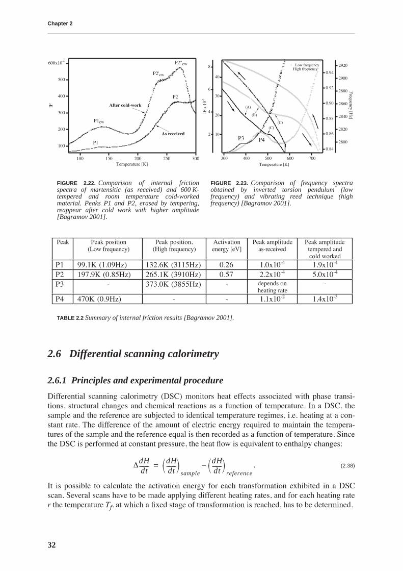
Chapter 2
32
2.6 Differential scanning calorimetry
2.6.1 Principles and experimental procedure
Differential scanning calorimetry (DSC) monitors heat effects associated with phase transi-tions, structural changes and chemical reactions as a function of temperature. In a DSC, thesample and the reference are subjected to identical temperature regimes, i.e. heating at a con-stant rate. The difference of the amount of electric energy required to maintain the tempera-tures of the sample and the reference equal is then recorded as a function of temperature. Sincethe DSC is performed at constant pressure, the heat flow is equivalent to enthalpy changes:
. (2.38)
It is possible to calculate the activation energy for each transformation exhibited in a DSCscan. Several scans have to be made applying different heating rates, and for each heating rater the temperature Tf, at which a fixed stage of transformation is reached, has to be determined.
FIGURE 2.22. Comparison of internal frictionspectra of martensitic (as received) and 600 K-tempered and room temperature cold-workedmaterial. Peaks P1 and P2, erased by tempering,reappear after cold work with higher amplitude[Bagramov 2001].
FIGURE 2.23. Comparison of frequency spectraobtained by inverted torsion pendulum (lowfrequency) and vibrating reed technique (highfrequency) [Bagramov 2001].
TABLE 2.2 Summary of internal friction results [Bagramov 2001].
600x10-6
500
400
300
200
100
IF
300250200150100Temperature [K]
As received
After cold-work
P1
P1cw
P2
P2"cw
P2'cw 0.94
0.92
0.90
0.88
0.86
0.84
700600500400300Temperature [K]
2920
2900
2880
2860
2840
2820
2800
Frequency [Hz]
40
30
20
10
IF x
10-3
8
6
4
2
Low frequencyHigh frequency
(A)
(B)
(C)(C)
P3 P4
Peak Peak position(Low frequency)
Peak position,(High frequency)
Activationenergy [eV]
Peak amplitudeas-received
Peak amplitudetempered andcold worked
P1 99.1K (1.09Hz) 132.6K (3115Hz) 0.26 1.0x10⁻⁴ 1.9x10⁻⁴
P2 197.9K (0.85Hz) 265.1K (3910Hz) 0.57 2.2x10⁻⁴ 5.0x10⁻⁴
P3 - 373.0K (3855Hz) - depends onheating rate
-
P4 470K (0.9Hz) - - 1.1x10⁻² 1.4x10⁻³
∆dHdt-------
dHdt-------⎝ ⎠⎛ ⎞
sample
dHdt-------⎝ ⎠⎛ ⎞
reference–=
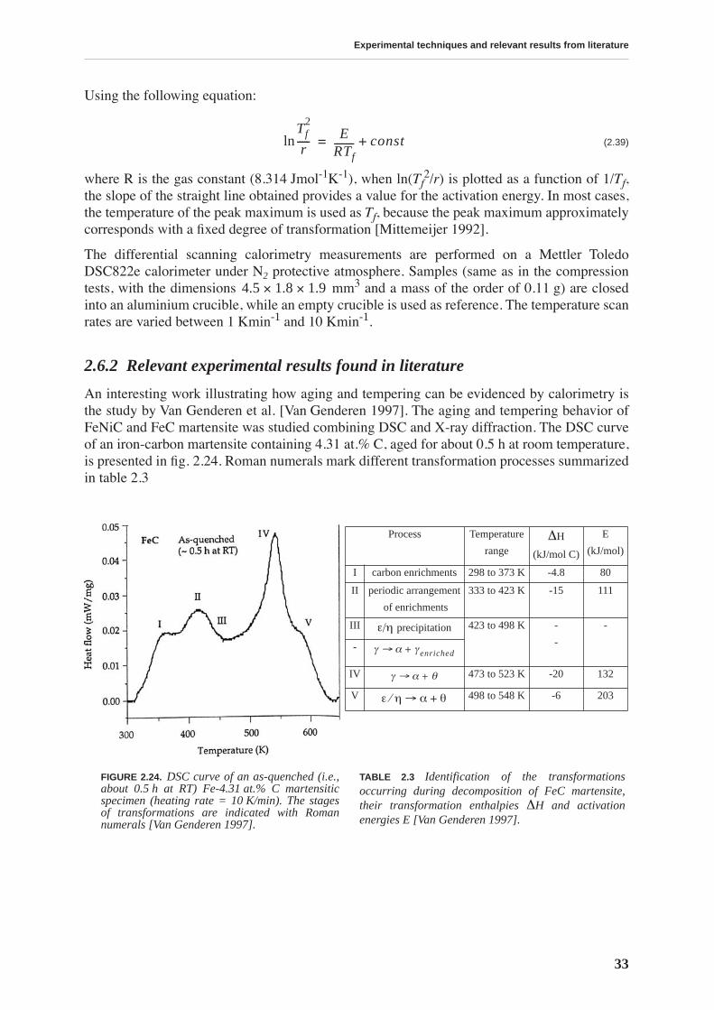
Experimental techniques and relevant results from literature
33
Using the following equation:
(2.39)
where R is the gas constant (8.314 Jmol-1K-1), when ln(Tf2/r) is plotted as a function of 1/Tf,
the slope of the straight line obtained provides a value for the activation energy. In most cases,the temperature of the peak maximum is used as Tf, because the peak maximum approximatelycorresponds with a fixed degree of transformation [Mittemeijer 1992].
The differential scanning calorimetry measurements are performed on a Mettler ToledoDSC822e calorimeter under N2 protective atmosphere. Samples (same as in the compressiontests, with the dimensions mm3 and a mass of the order of 0.11 g) are closedinto an aluminium crucible, while an empty crucible is used as reference. The temperature scanrates are varied between 1 Kmin-1 and 10 Kmin-1.
2.6.2 Relevant experimental results found in literature
An interesting work illustrating how aging and tempering can be evidenced by calorimetry isthe study by Van Genderen et al. [Van Genderen 1997]. The aging and tempering behavior ofFeNiC and FeC martensite was studied combining DSC and X-ray diffraction. The DSC curveof an iron-carbon martensite containing 4.31 at.% C, aged for about 0.5 h at room temperature,is presented in fig. 2.24. Roman numerals mark different transformation processes summarizedin table 2.3
FIGURE 2.24. DSC curve of an as-quenched (i.e.,about 0.5 h at RT) Fe-4.31 at.% C martensiticspecimen (heating rate = 10 K/min). The stagesof transformations are indicated with Romannumerals [Van Genderen 1997].
TABLE 2.3 Identification of the transformationsoccurring during decomposition of FeC martensite,their transformation enthalpies ∆H and activationenergies E [Van Genderen 1997].
Tf2
r-----ln E
RTf-------- const+=
4.5 1.8 1.9××
Process Temperature
range∆H
(kJ/mol C)
E
(kJ/mol)
I carbon enrichments 298 to 373 K -4.8 80
II periodic arrangement
of enrichments
333 to 423 K -15 111
III ε/η precipitation 423 to 498 K -
-
-
-
IV 473 to 523 K -20 132
V 498 to 548 K -6 203
γ α γ enriched+→
γ α θ+→
ε η⁄ α θ+→

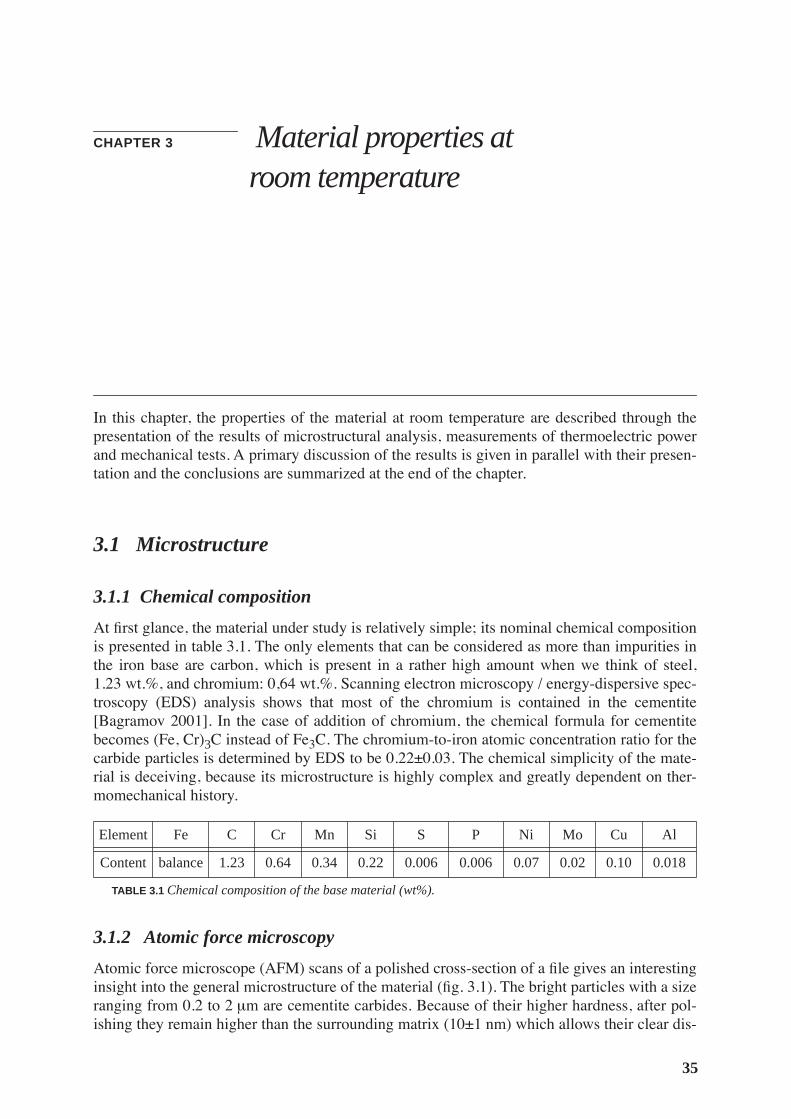
35
CHAPTER 3
Material properties at room temperature
In this chapter, the properties of the material at room temperature are described through thepresentation of the results of microstructural analysis, measurements of thermoelectric powerand mechanical tests. A primary discussion of the results is given in parallel with their presen-tation and the conclusions are summarized at the end of the chapter.
3.1 Microstructure
3.1.1 Chemical composition
At first glance, the material under study is relatively simple; its nominal chemical compositionis presented in table 3.1. The only elements that can be considered as more than impurities inthe iron base are carbon, which is present in a rather high amount when we think of steel,1.23 wt.%, and chromium: 0,64 wt.%. Scanning electron microscopy / energy-dispersive spec-troscopy (EDS) analysis shows that most of the chromium is contained in the cementite[Bagramov 2001]. In the case of addition of chromium, the chemical formula for cementitebecomes (Fe, Cr)
3
C instead of Fe
3
C. The chromium-to-iron atomic concentration ratio for thecarbide particles is determined by EDS to be 0.22±0.03. The chemical simplicity of the mate-rial is deceiving, because its microstructure is highly complex and greatly dependent on ther-momechanical history.
3.1.2 Atomic force microscopy
Atomic force microscope (AFM) scans of a polished cross-section of a file gives an interestinginsight into the general microstructure of the material (fig. 3.1). The bright particles with a sizeranging from 0.2 to 2
µ
m are cementite carbides. Because of their higher hardness, after pol-ishing they remain higher than the surrounding matrix (10±1 nm) which allows their clear dis-
Element Fe C Cr Mn Si S P Ni Mo Cu Al
Content balance 1.23 0.64 0.34 0.22 0.006 0.006 0.07 0.02 0.10 0.018
TABLE 3.1
Chemical composition of the base material (wt%).
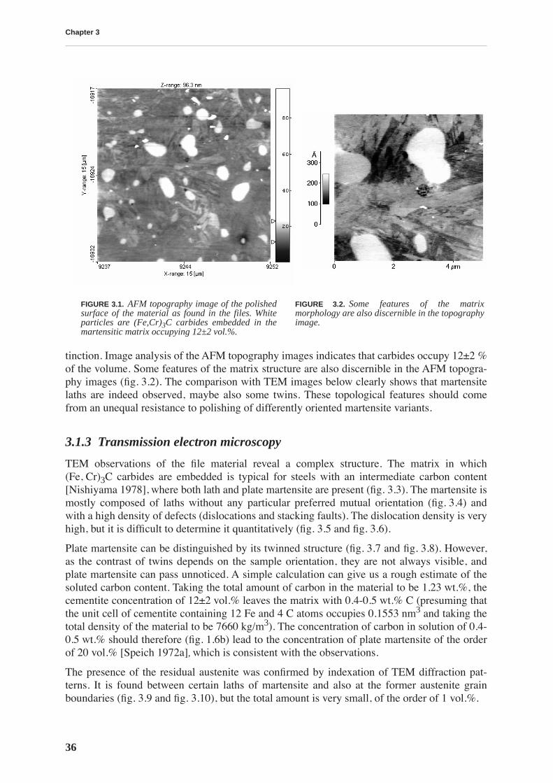
Chapter 3
36
tinction. Image analysis of the AFM topography images indicates that carbides occupy 12±2 %of the volume. Some features of the matrix structure are also discernible in the AFM topogra-phy images (fig. 3.2). The comparison with TEM images below clearly shows that martensitelaths are indeed observed, maybe also some twins. These topological features should comefrom an unequal resistance to polishing of differently oriented martensite variants.
3.1.3 Transmission electron microscopy
TEM observations of the file material reveal a complex structure. The matrix in which(Fe, Cr)
3
C carbides are embedded is typical for steels with an intermediate carbon content[Nishiyama 1978],
where both lath and plate martensite are present (fig. 3.3). The martensite ismostly composed of laths without any particular preferred mutual orientation (fig. 3.4) andwith a high density of defects (dislocations and stacking faults). The dislocation density is veryhigh, but it is difficult to determine it quantitatively (fig. 3.5 and fig. 3.6).
Plate martensite can be distinguished by its twinned structure (fig. 3.7 and fig. 3.8). However,as the contrast of twins depends on the sample orientation, they are not always visible, andplate martensite can pass unnoticed. A simple calculation can give us a rough estimate of thesoluted carbon content. Taking the total amount of carbon in the material to be 1.23 wt.%, thecementite concentration of 12±2 vol.% leaves the matrix with 0.4-0.5 wt.% C (presuming thatthe unit cell of cementite containing 12 Fe and 4 C atoms occupies 0.1553 nm
3
and taking thetotal density of the material to be 7660 kg/m
3
). The concentration of carbon in solution of 0.4-0.5 wt.% should therefore (fig. 1.6b) lead to the concentration of plate martensite of the orderof 20 vol.% [Speich 1972a]
,
which is consistent with the observations.
The presence of the residual austenite was confirmed by indexation of TEM diffraction pat-terns. It is found between certain laths of martensite and also at the former austenite grainboundaries (fig. 3.9 and fig. 3.10), but the total amount is very small, of the order of 1 vol.%.
FIGURE 3.1.
AFM topography image of the polishedsurface of the material as found in the files. Whiteparticles are (Fe,Cr)
3
C carbides embedded in themartensitic matrix occupying 12±2 vol.%.
FIGURE 3.2.
Some features of the matrixmorphology are also discernible in the topographyimage.
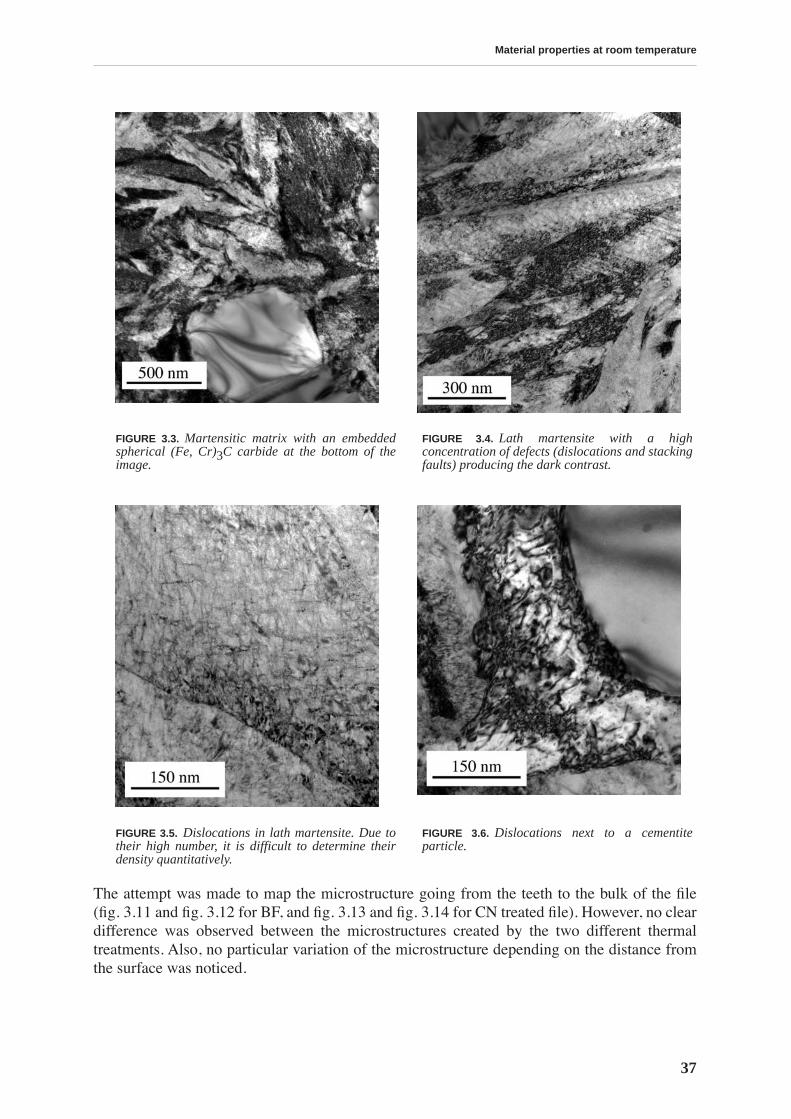
Material properties at room temperature
37
The attempt was made to map the microstructure going from the teeth to the bulk of the file(fig. 3.11 and fig. 3.12 for BF, and fig. 3.13 and fig. 3.14 for CN treated file). However, no cleardifference was observed between the microstructures created by the two different thermaltreatments. Also, no particular variation of the microstructure depending on the distance fromthe surface was noticed.
FIGURE 3.3.
Martensitic matrix with an embeddedspherical (Fe, Cr)
3
C carbide at the bottom of theimage.
FIGURE 3.4.
Lath martensite with a highconcentration of defects (dislocations and stackingfaults) producing the dark contrast.
FIGURE 3.5.
Dislocations in lath martensite. Due totheir high number, it is difficult to determine theirdensity quantitatively.
FIGURE 3.6.
Dislocations next to a cementiteparticle.
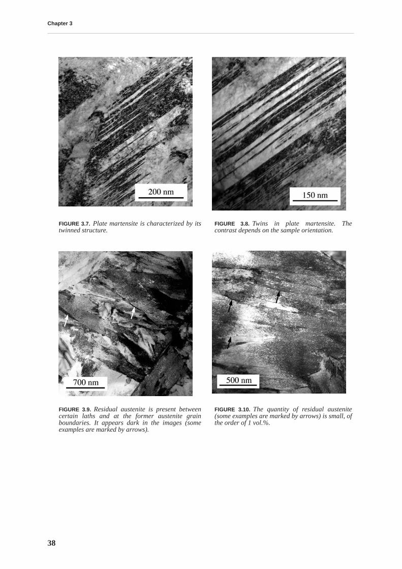
Chapter 3
38
FIGURE 3.7.
Plate martensite is characterized by itstwinned structure.
FIGURE 3.8.
Twins in plate martensite. Thecontrast depends on the sample orientation.
FIGURE 3.9.
Residual austenite is present betweencertain laths and at the former austenite grainboundaries. It appears dark in the images (someexamples are marked by arrows).
FIGURE 3.10.
The quantity of residual austenite(some examples are marked by arrows) is small, ofthe order of 1 vol.%.
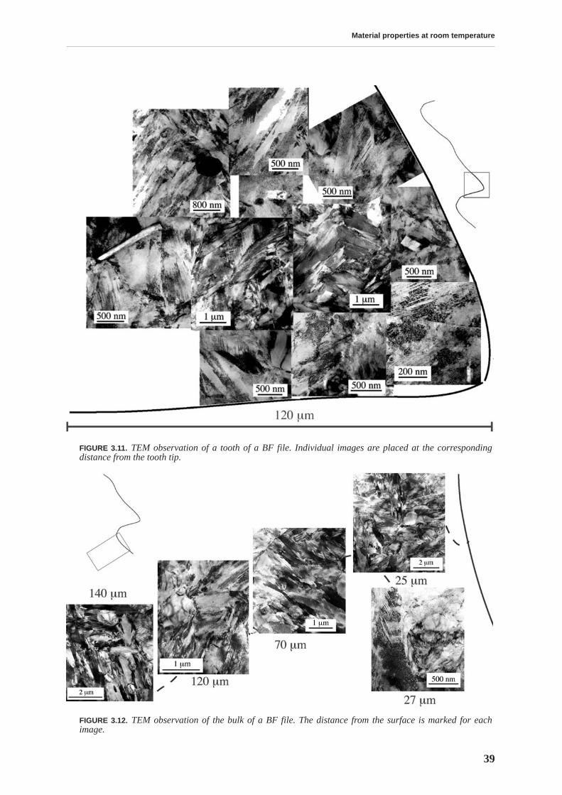
Material properties at room temperature
39
FIGURE 3.11.
TEM observation of a tooth of a BF file. Individual images are placed at the correspondingdistance from the tooth tip.
FIGURE 3.12.
TEM observation of the bulk of a BF file. The distance from the surface is marked for eachimage.
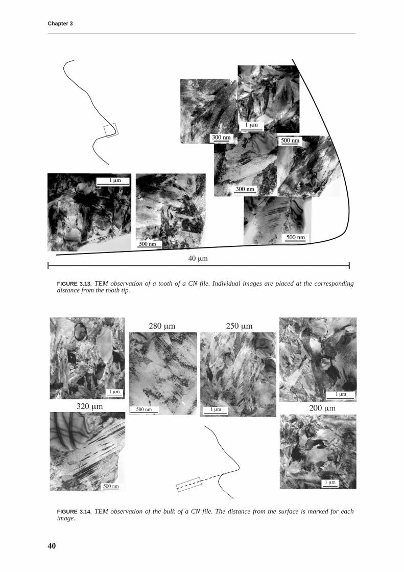
Chapter 3
40
FIGURE 3.13.
TEM observation of a tooth of a CN file. Individual images are placed at the correspondingdistance from the tooth tip.
FIGURE 3.14.
TEM observation of the bulk of a CN file. The distance from the surface is marked for eachimage.
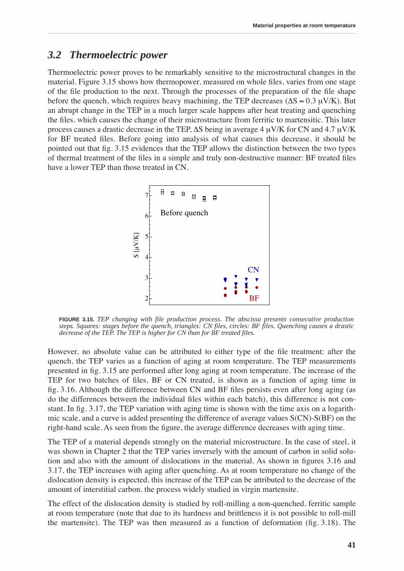
Material properties at room temperature
41
3.2 Thermoelectric power
Thermoelectric power proves to be remarkably sensitive to the microstructural changes in thematerial. Figure 3.15 shows how thermopower, measured on whole files, varies from one stageof the file production to the next. Through the processes of the preparation of the file shapebefore the quench, which requires heavy machining, the TEP decreases (
∆
S
≈
0.3
µ
V/K). Butan abrupt change in the TEP in a much larger scale happens after heat treating and quenchingthe files, which causes the change of their microstructure from ferritic to martensitic. This laterprocess causes a drastic decrease in the TEP,
∆
S being in average 4
µ
V/K for CN and 4.7
µ
V/Kfor BF treated files. Before going into analysis of what causes this decrease, it should bepointed out that fig. 3.15 evidences that the TEP allows the distinction between the two typesof thermal treatment of the files in a simple and truly non-destructive manner: BF treated fileshave a lower TEP than those treated in CN.
However, no absolute value can be attributed to either type of the file treatment: after thequench, the TEP varies as a function of aging at room temperature. The TEP measurementspresented in fig. 3.15 are performed after long aging at room temperature. The increase of theTEP for two batches of files, BF or CN treated, is shown as a function of aging time infig. 3.16. Although the difference between CN and BF files persists even after long aging (asdo the differences between the individual files within each batch), this difference is not con-stant. In fig. 3.17, the TEP variation with aging time is shown with the time axis on a logarith-mic scale, and a curve is added presenting the difference of average values S(CN)-S(BF) on theright-hand scale. As seen from the figure, the average difference decreases with aging time.
The TEP of a material depends strongly on the material microstructure. In the case of steel, itwas shown in Chapter 2 that the TEP varies inversely with the amount of carbon in solid solu-tion and also with the amount of dislocations in the material. As shown in figures 3.16 and3.17, the TEP increases with aging after quenching. As at room temperature no change of thedislocation density is expected, this increase of the TEP can be attributed to the decrease of theamount of interstitial carbon, the process widely studied in virgin martensite.
The effect of the dislocation density is studied by roll-milling a non-quenched, ferritic sampleat room temperature (note that due to its hardness and brittleness it is not possible to roll-millthe martensite). The TEP was then measured as a function of deformation (fig. 3.18). The
FIGURE 3.15.
TEP changing with file production process. The abscissa presents consecutive productionsteps. Squares: stages before the quench, triangles: CN files, circles: BF files. Quenching causes a drasticdecrease of the TEP. The TEP is higher for CN than for BF treated files.
7
6
5
4
3
2
S [µ
V/K
]
Before quench
BF
CN
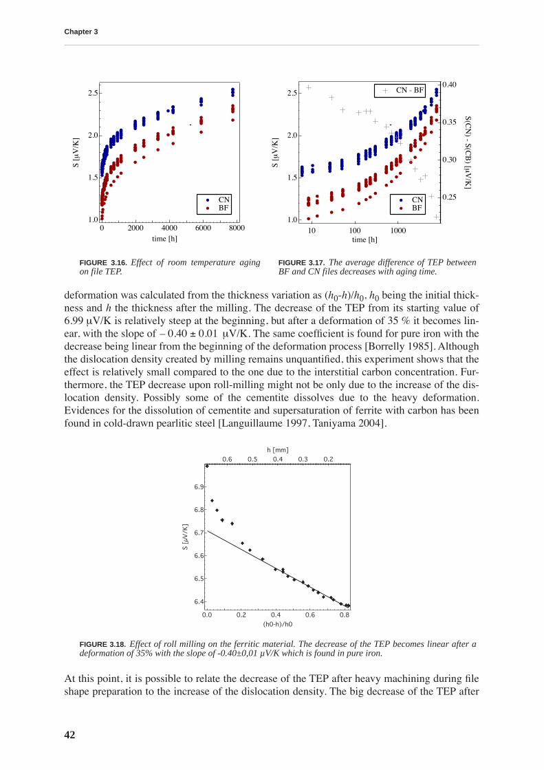
Chapter 3
42
deformation was calculated from the thickness variation as (
h
0
-
h
)/
h
0
,
h
0
being the initial thick-ness and
h
the thickness after the milling. The decrease of the TEP from its starting value of6.99
µ
V/K is relatively steep at the beginning, but after a deformation of 35 % it becomes lin-ear, with the slope of
µ
V/K. The same coefficient is found for pure iron with thedecrease being linear from the beginning of the deformation process [Borrelly 1985]. Althoughthe dislocation density created by milling remains unquantified, this experiment shows that theeffect is relatively small compared to the one due to the interstitial carbon concentration. Fur-thermore, the TEP decrease upon roll-milling might not be only due to the increase of the dis-location density. Possibly some of the cementite dissolves due to the heavy deformation.Evidences for the dissolution of cementite and supersaturation of ferrite with carbon has beenfound in cold-drawn pearlitic steel [Languillaume 1997, Taniyama 2004].
At this point, it is possible to relate the decrease of the TEP after heavy machining during fileshape preparation to the increase of the dislocation density. The big decrease of the TEP after
FIGURE 3.16.
Effect of room temperature agingon file TEP.
FIGURE 3.17.
The average difference of TEP betweenBF and CN files decreases with aging time.
FIGURE 3.18.
Effect of roll milling on the ferritic material. The decrease of the TEP becomes linear after adeformation of 35% with the slope of -0.40±0,01 µV/K which is found in pure iron.
2.5
2.0
1.5
1.0
S [µ
V/K
]
80006000400020000time [h]
CN BF
2.5
2.0
1.5
1.0
S [µ
V/K
]
10 100 1000time [h]
0.40
0.35
0.30
0.25
S(CN
) - S(CB
) [µV
/K]
CN BF
CN - BF
0.40– 0.01±
6.9
6.8
6.7
6.6
6.5
6.4
S [µ
V/K
]
0.80.60.40.20.0(h0-h)/h0
0.6 0.5 0.4 0.3 0.2h [mm]
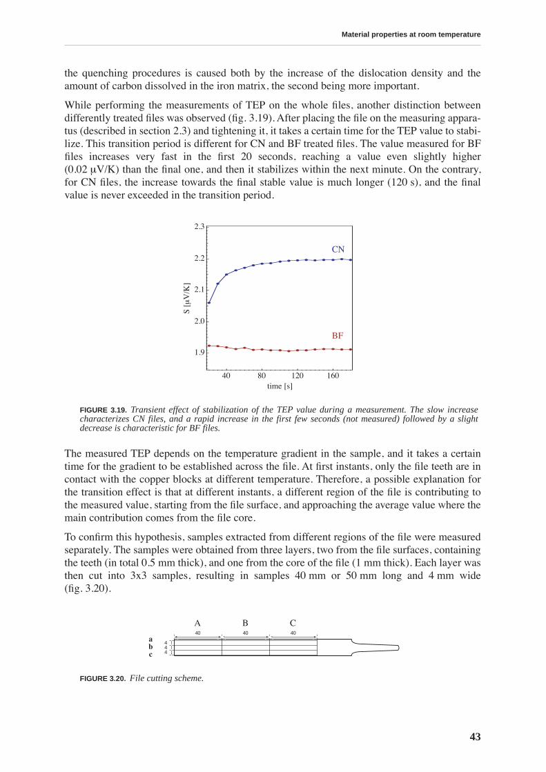
Material properties at room temperature
43
the quenching procedures is caused both by the increase of the dislocation density and theamount of carbon dissolved in the iron matrix, the second being more important.
While performing the measurements of TEP on the whole files, another distinction betweendifferently treated files was observed (fig. 3.19). After placing the file on the measuring appara-tus (described in section 2.3) and tightening it, it takes a certain time for the TEP value to stabi-lize. This transition period is different for CN and BF treated files. The value measured for BFfiles increases very fast in the first 20 seconds, reaching a value even slightly higher(0.02
µ
V/K) than the final one, and then it stabilizes within the next minute. On the contrary,for CN files, the increase towards the final stable value is much longer (120 s), and the finalvalue is never exceeded in the transition period.
The measured TEP depends on the temperature gradient in the sample, and it takes a certaintime for the gradient to be established across the file. At first instants, only the file teeth are incontact with the copper blocks at different temperature. Therefore, a possible explanation forthe transition effect is that at different instants, a different region of the file is contributing tothe measured value, starting from the file surface, and approaching the average value where themain contribution comes from the file core.
To confirm this hypothesis, samples extracted from different regions of the file were measuredseparately. The samples were obtained from three layers, two from the file surfaces, containingthe teeth (in total 0.5 mm thick), and one from the core of the file (1 mm thick). Each layer wasthen cut into 3x3 samples, resulting in samples 40 mm or 50 mm long and 4 mm wide(fig. 3.20).
FIGURE 3.19.
Transient effect of stabilization of the TEP value during a measurement. The slow increasecharacterizes CN files, and a rapid increase in the first few seconds (not measured) followed by a slightdecrease is characteristic for BF files.
FIGURE 3.20.
File cutting scheme.
2.3
2.2
2.1
2.0
1.9
1601208040time [s]
S [µ
V/K
]
BF
CN
A B C
abc 4
44
40 40 40
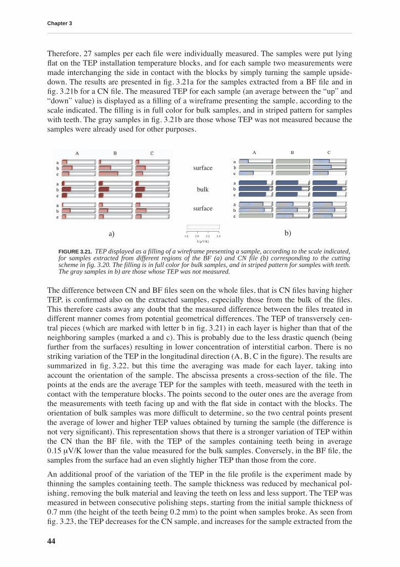
Chapter 3
44
Therefore, 27 samples per each file were individually measured. The samples were put lyingflat on the TEP installation temperature blocks, and for each sample two measurements weremade interchanging the side in contact with the blocks by simply turning the sample upside-down. The results are presented in fig. 3.21a for the samples extracted from a BF file and infig. 3.21b for a CN file. The measured TEP for each sample (an average between the “up” and“down” value) is displayed as a filling of a wireframe presenting the sample, according to thescale indicated. The filling is in full color for bulk samples, and in striped pattern for sampleswith teeth. The gray samples in fig. 3.21b are those whose TEP was not measured because thesamples were already used for other purposes.
The difference between CN and BF files seen on the whole files, that is CN files having higherTEP, is confirmed also on the extracted samples, especially those from the bulk of the files.This therefore casts away any doubt that the measured difference between the files treated indifferent manner comes from potential geometrical differences. The TEP of transversely cen-tral pieces (which are marked with letter b in fig. 3.21) in each layer is higher than that of theneighboring samples (marked a and c). This is probably due to the less drastic quench (beingfurther from the surfaces) resulting in lower concentration of interstitial carbon. There is nostriking variation of the TEP in the longitudinal direction (A, B, C in the figure). The results aresummarized in fig. 3.22, but this time the averaging was made for each layer, taking intoaccount the orientation of the sample. The abscissa presents a cross-section of the file. Thepoints at the ends are the average TEP for the samples with teeth, measured with the teeth incontact with the temperature blocks. The points second to the outer ones are the average fromthe measurements with teeth facing up and with the flat side in contact with the blocks. Theorientation of bulk samples was more difficult to determine, so the two central points presentthe average of lower and higher TEP values obtained by turning the sample (the difference isnot very significant). This representation shows that there is a stronger variation of TEP withinthe CN than the BF file, with the TEP of the samples containing teeth being in average0.15
µ
V/K lower than the value measured for the bulk samples. Conversely, in the BF file, thesamples from the surface had an even slightly higher TEP than those from the core.
An additional proof of the variation of the TEP in the file profile is the experiment made bythinning the samples containing teeth. The sample thickness was reduced by mechanical pol-ishing, removing the bulk material and leaving the teeth on less and less support. The TEP wasmeasured in between consecutive polishing steps, starting from the initial sample thickness of0.7 mm (the height of the teeth being 0.2 mm) to the point when samples broke. As seen fromfig. 3.23, the TEP decreases for the CN sample, and increases for the sample extracted from the
a)
b)
FIGURE 3.21.
TEP displayed as a filling of a wireframe presenting a sample, according to the scale indicated,for samples extracted from different regions of the BF (a) and CN file (b) corresponding to the cuttingscheme in fig. 3.20. The filling is in full color for bulk samples, and in striped pattern for samples with teeth.The gray samples in b) are those whose TEP was not measured.
surface
bulk
surface
1.8 2.0 2.2 2.4
S [µV/K]
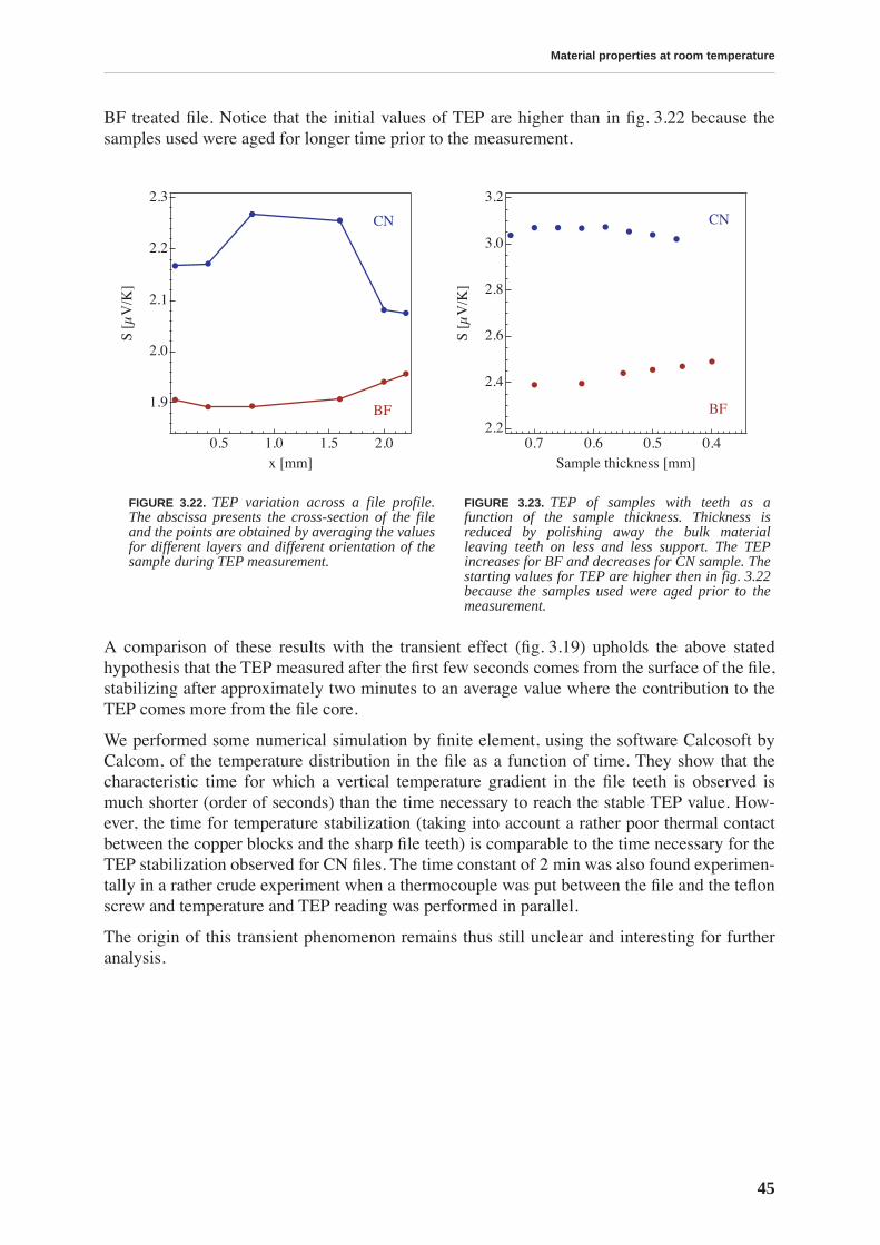
Material properties at room temperature
45
BF treated file. Notice that the initial values of TEP are higher than in fig. 3.22 because thesamples used were aged for longer time prior to the measurement.
A comparison of these results with the transient effect (fig. 3.19) upholds the above statedhypothesis that the TEP measured after the first few seconds comes from the surface of the file,stabilizing after approximately two minutes to an average value where the contribution to theTEP comes more from the file core.
We performed some numerical simulation by finite element, using the software Calcosoft byCalcom, of the temperature distribution in the file as a function of time. They show that thecharacteristic time for which a vertical temperature gradient in the file teeth is observed ismuch shorter (order of seconds) than the time necessary to reach the stable TEP value. How-ever, the time for temperature stabilization (taking into account a rather poor thermal contactbetween the copper blocks and the sharp file teeth) is comparable to the time necessary for theTEP stabilization observed for CN files. The time constant of 2 min was also found experimen-tally in a rather crude experiment when a thermocouple was put between the file and the teflonscrew and temperature and TEP reading was performed in parallel.
The origin of this transient phenomenon remains thus still unclear and interesting for furtheranalysis.
FIGURE 3.22.
TEP variation across a file profile.The abscissa presents the cross-section of the fileand the points are obtained by averaging the valuesfor different layers and different orientation of thesample during TEP measurement.
FIGURE 3.23.
TEP of samples with teeth as afunction of the sample thickness. Thickness isreduced by polishing away the bulk materialleaving teeth on less and less support. The TEPincreases for BF and decreases for CN sample. Thestarting values for TEP are higher then in fig. 3.22because the samples used were aged prior to themeasurement.
2.3
2.2
2.1
2.0
1.9
S [µ
V/K
]
2.01.51.00.5x [mm]
BF
CN
3.2
3.0
2.8
2.6
2.4
2.2
S [µ
V/K
]0.7 0.6 0.5 0.4
Sample thickness [mm]
BF
CN
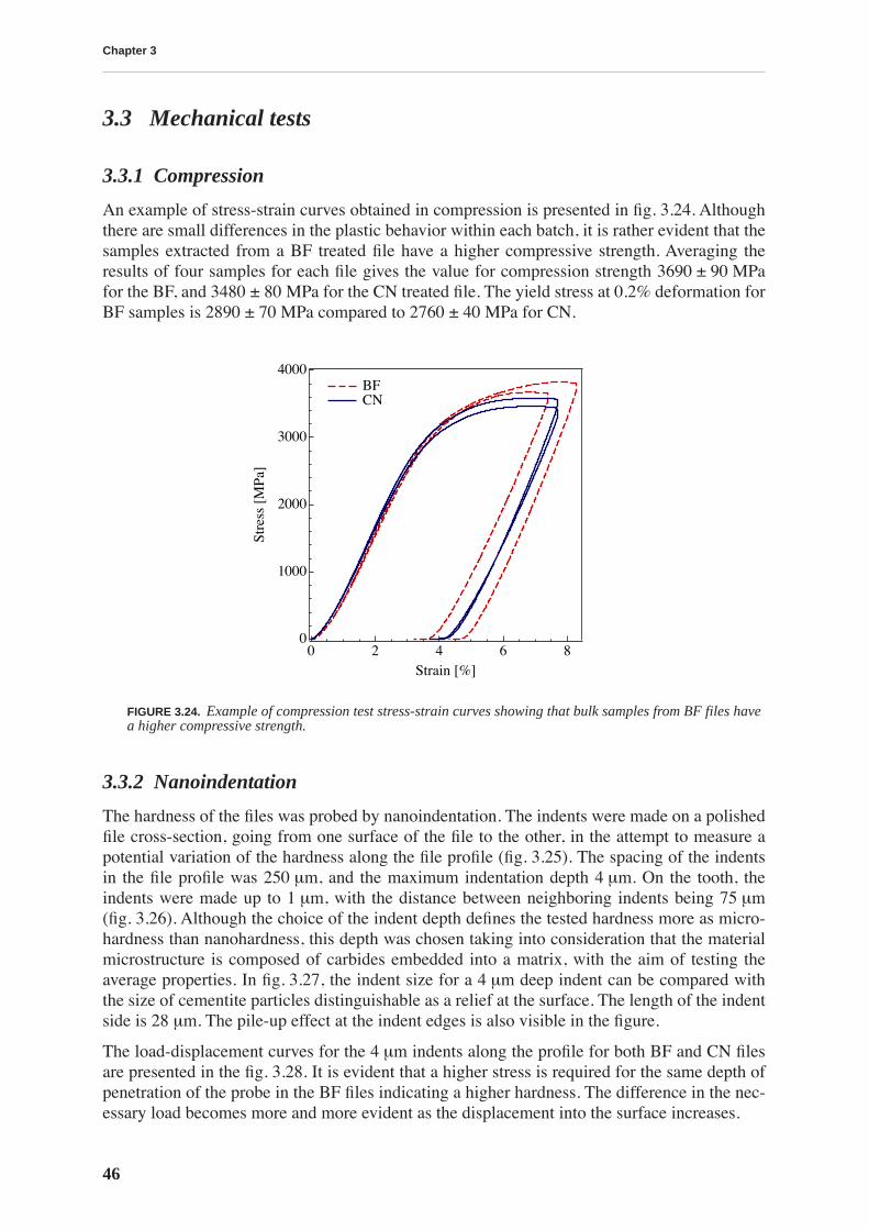
Chapter 3
46
3.3 Mechanical tests
3.3.1 Compression
An example of stress-strain curves obtained in compression is presented in fig. 3.24. Althoughthere are small differences in the plastic behavior within each batch, it is rather evident that thesamples extracted from a BF treated file have a higher compressive strength. Averaging theresults of four samples for each file gives the value for compression strength 3690 ± 90 MPafor the BF, and 3480 ± 80 MPa for the CN treated file. The yield stress at 0.2% deformation forBF samples is 2890 ± 70 MPa compared to 2760 ± 40 MPa for CN.
3.3.2 Nanoindentation
The hardness of the files was probed by nanoindentation. The indents were made on a polishedfile cross-section, going from one surface of the file to the other, in the attempt to measure apotential variation of the hardness along the file profile (fig. 3.25). The spacing of the indentsin the file profile was 250
µ
m, and the maximum indentation depth 4
µ
m. On the tooth, theindents were made up to 1
µ
m, with the distance between neighboring indents being 75
µ
m(fig. 3.26). Although the choice of the indent depth defines the tested hardness more as micro-hardness than nanohardness, this depth was chosen taking into consideration that the materialmicrostructure is composed of carbides embedded into a matrix, with the aim of testing theaverage properties. In fig. 3.27, the indent size for a 4
µ
m deep indent can be compared withthe size of cementite particles distinguishable as a relief at the surface. The length of the indentside is 28
µ
m. The pile-up effect at the indent edges is also visible in the figure.
The load-displacement curves for the 4
µ
m indents along the profile for both BF and CN filesare presented in the fig. 3.28. It is evident that a higher stress is required for the same depth ofpenetration of the probe in the BF files indicating a higher hardness. The difference in the nec-essary load becomes more and more evident as the displacement into the surface increases.
FIGURE 3.24.
Example of compression test stress-strain curves showing that bulk samples from BF files havea higher compressive strength.
4000
3000
2000
1000
0
Stre
ss [
MPa
]
86420Strain [%]
BF CN

Material properties at room temperature
47
The hardness measured by the continuous stiffness method during the loading is shown infig. 3.29a as a function of the penetration depth. The measurements become meaningful onlyfor a displacement into the surface higher than 500 nm, below this value the effects of structureinhomogeneity lead to a huge scatter. As seen from the graph, BF treated files have a higherhardness. The hardness, averaged for the indenter displacement into the surface between 1000and 1200 nm and then over all indents, is 11.3±0.3 GPa for the CN and 11.6±0.2 GPa for theBF treated file. However, no variation of the hardness is observed as a function of the distancefrom the file surface due to the large fluctuations in the measured value. The region closer than50
µ
m from the surface could not have been tested successfully with 4
µ
m deep indents, due totooth edge effects.
The elastic modulus measured by the continuous stiffness method is presented in fig. 3.29b. Asfor the hardness, the fluctuations of the measured values impede the determination of the possi-ble variations along the file profile, but it is possible to say that in average we measure a highermodulus for the BF than for the CN treated file. The average, obtained in the same manner as
FIGURE 3.25.
Optical microscope image of a series ofindents made in the file profile (to the depth of 4
µ
m). Theindents are 250
µ
m apart.
FIGURE 3.26.
Placing of the indents on the filetooth. The distance between the indents is75 µm and the indentation depth 1 µm.
FIGURE 3.27. Optical microscope image of the indent made in the bulk of the file (CN). The length of theindent side of 28 µm can be compared with the size of cementite particles that appear as a relief due to thelight interference contrast. The pile-up effect at the indent edges is also visible.
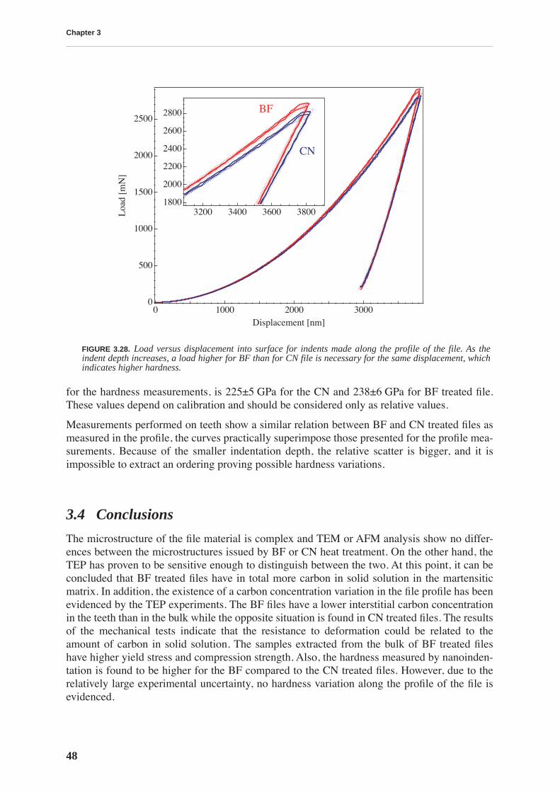
Chapter 3
48
for the hardness measurements, is 225±5 GPa for the CN and 238±6 GPa for BF treated file.These values depend on calibration and should be considered only as relative values.
Measurements performed on teeth show a similar relation between BF and CN treated files asmeasured in the profile, the curves practically superimpose those presented for the profile mea-surements. Because of the smaller indentation depth, the relative scatter is bigger, and it isimpossible to extract an ordering proving possible hardness variations.
3.4 Conclusions
The microstructure of the file material is complex and TEM or AFM analysis show no differ-ences between the microstructures issued by BF or CN heat treatment. On the other hand, theTEP has proven to be sensitive enough to distinguish between the two. At this point, it can beconcluded that BF treated files have in total more carbon in solid solution in the martensiticmatrix. In addition, the existence of a carbon concentration variation in the file profile has beenevidenced by the TEP experiments. The BF files have a lower interstitial carbon concentrationin the teeth than in the bulk while the opposite situation is found in CN treated files. The resultsof the mechanical tests indicate that the resistance to deformation could be related to theamount of carbon in solid solution. The samples extracted from the bulk of BF treated fileshave higher yield stress and compression strength. Also, the hardness measured by nanoinden-tation is found to be higher for the BF compared to the CN treated files. However, due to therelatively large experimental uncertainty, no hardness variation along the profile of the file isevidenced.
FIGURE 3.28. Load versus displacement into surface for indents made along the profile of the file. As theindent depth increases, a load higher for BF than for CN file is necessary for the same displacement, whichindicates higher hardness.
2500
2000
1500
1000
500
0
Loa
d [m
N]
3000200010000Displacement [nm]
2800
2600
2400
2200
2000
18003800360034003200
BF
CN
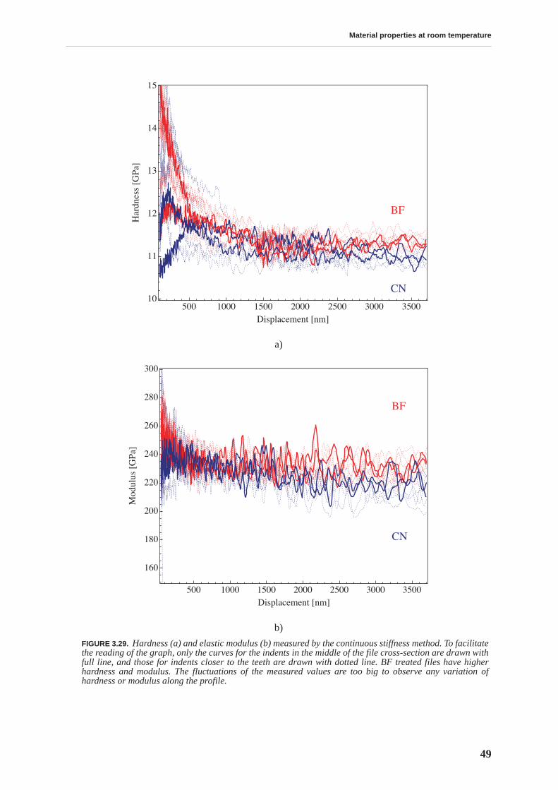
Material properties at room temperature
49
a)
b)
FIGURE 3.29. Hardness (a) and elastic modulus (b) measured by the continuous stiffness method. To facilitatethe reading of the graph, only the curves for the indents in the middle of the file cross-section are drawn withfull line, and those for indents closer to the teeth are drawn with dotted line. BF treated files have higherhardness and modulus. The fluctuations of the measured values are too big to observe any variation ofhardness or modulus along the profile.
15
14
13
12
11
10
Har
dnes
s [G
Pa]
350030002500200015001000500Displacement [nm]
BF
CN
300
280
260
240
220
200
180
160
Mod
ulus
[G
Pa]
350030002500200015001000500Displacement [nm]
BF
CN

51
CHAPTER 4
Mechanical spectroscopy
The results presented in the previous chapter emphasize the importance of interstitial carbonfor the mechanical properties of the material, namely its hardness and strength. Mechanicalspectroscopy is known to be a very sensitive indicator of the interactions of soluted atoms withdislocations and of their mobility, and it is thus chosen as a technique to get a better insight intothese mechanisms, which are also responsible for the macroscopic mechanical properties ofthe material.
4.1 Temperature spectra
4.1.1 High and low frequency spectra for martensite
The typical internal friction and frequency spectrum, measured in the vibrating reed installa-tion during a first heating of a martensitic sample and then in cooling after 1 h of tempering at800 K, is shown in the fig. 4.1. The differences in internal friction spectra for the samplesextracted from files that underwent different thermal treatments are very small (not visible inthis scale), and will be discussed separately. The IF spectrum obtained in heating can bedecomposed into five broadened Debye shaped peaks and an exponential background [Mari1999], as presented in fig. 4.2. The parameters of the peaks, i.e. peak amplitude, temperature,activation energy and broadening factor, as obtained by a peak fitting procedure, are listed inthe same figure.
A typical internal friction and frequency measurement performed in the inverted torsion pen-dulum during heating, 1 h tempering at 700 K and the following cooling of the initially mar-tensitic sample is presented in fig. 4.3. The equivalent decomposition into broadened Debyeshaped peaks (without the peak P1 which is not distinguishable in the spectrum) and an expo-nential background is presented in fig. 4.4.
A comparison of the internal friction spectra obtained in both installations reveal that four ofthe peaks found in the spectrum are thermally activated: the temperatures of the peaks P1, P2,P4 and P5 depend strongly on the measurement frequency. The activation energy and theattempt frequency calculated for the thermally activated peaks according to eq. 2.27 are givenin table 4.1. The relaxation parameters for the peaks P2 and P5 are calculated based on 10
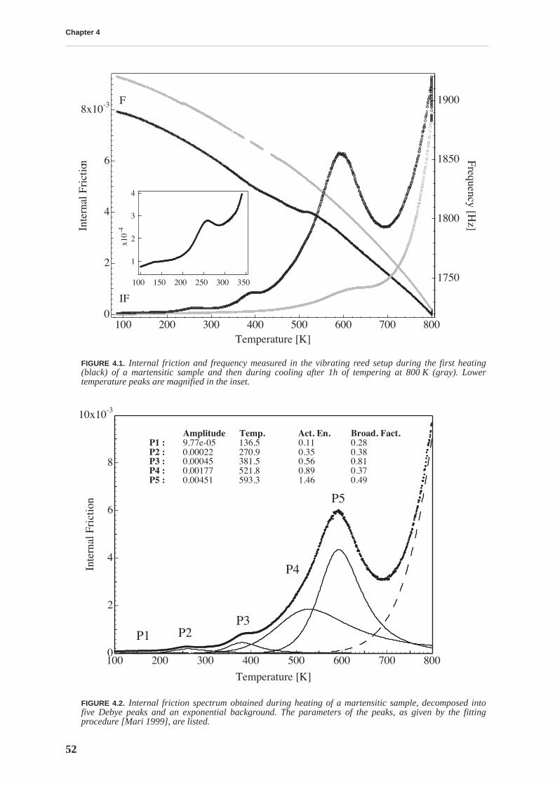
Chapter 4
52
FIGURE 4.1.
Internal friction and frequency measured in the vibrating reed setup during the first heating(black) of a martensitic sample and then during cooling after 1h of tempering at 800 K (gray). Lowertemperature peaks are magnified in the inset.
FIGURE 4.2.
Internal friction spectrum obtained during heating of a martensitic sample, decomposed intofive Debye peaks and an exponential background. The parameters of the peaks, as given by the fittingprocedure [Mari 1999], are listed.
1900
1850
1800
1750
Frequency [Hz]
800700600500400300200100Temperature [K]
8x10⁻³
6
4
2
0
Inte
rnal
Fri
ction
IF
F
4
3
2
1
x10
-4
350300250200150100
10x10-3
8
6
4
2
0
Inte
rnal
Fri
ctio
n
800700600500400300200100
Temperature [K]
P5
P4
P3P1 P2
Amplitude Temp. Act. En. Broad. Fact.P1 : 9.77e-05 136.5 0.11 0.28P2 : 0.00022 270.9 0.35 0.38P3 : 0.00045 381.5 0.56 0.81P4 : 0.00177 521.8 0.89 0.37P5 : 0.00451 593.3 1.46 0.49
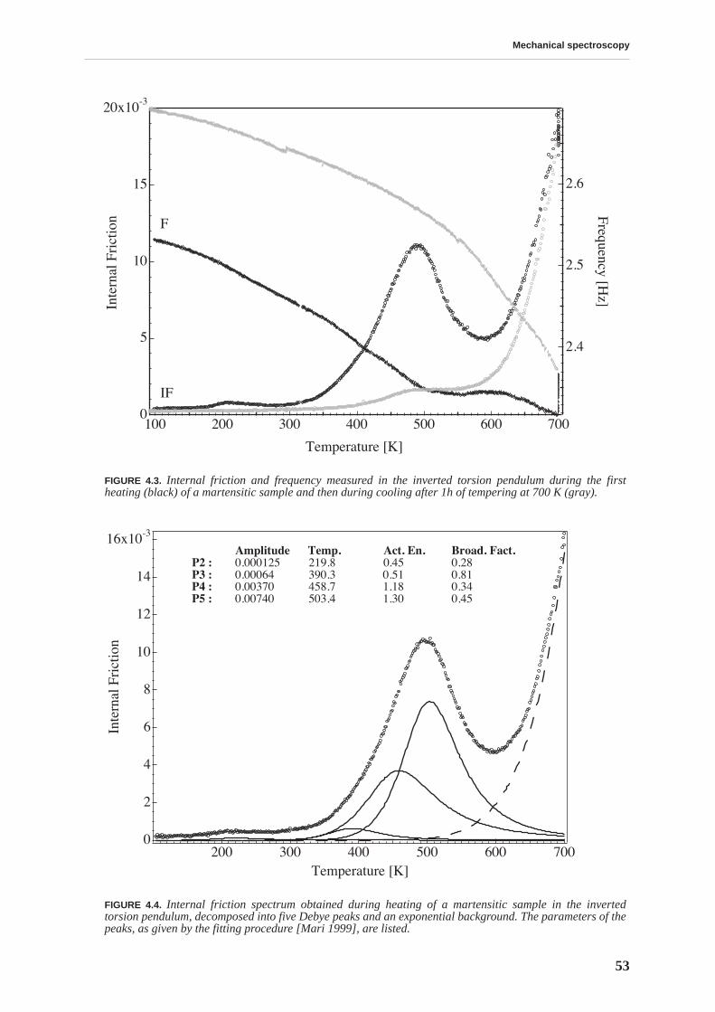
Mechanical spectroscopy
53
FIGURE 4.3.
Internal friction and frequency measured in the inverted torsion pendulum during the firstheating (black) of a martensitic sample and then during cooling after 1h of tempering at 700 K (gray).
FIGURE 4.4.
Internal friction spectrum obtained during heating of a martensitic sample in the invertedtorsion pendulum, decomposed into five Debye peaks and an exponential background. The parameters of thepeaks, as given by the fitting procedure [Mari 1999], are listed.
20x10-3
15
10
5
0
Inte
rnal
Fri
ctio
n
700600500400300200100
Temperature [K]
2.6
2.5
2.4
Frequency [Hz]
IF
F
16x10-3
14
12
10
8
6
4
2
0
Inte
rnal
Fri
ctio
n
700600500400300200Temperature [K]
Amplitude Temp. Act. En. Broad. Fact.P2 : 0.000125 219.8 0.45 0.28P3 : 0.00064 390.3 0.51 0.81P4 : 0.00370 458.7 1.18 0.34P5 : 0.00740 503.4 1.30 0.45
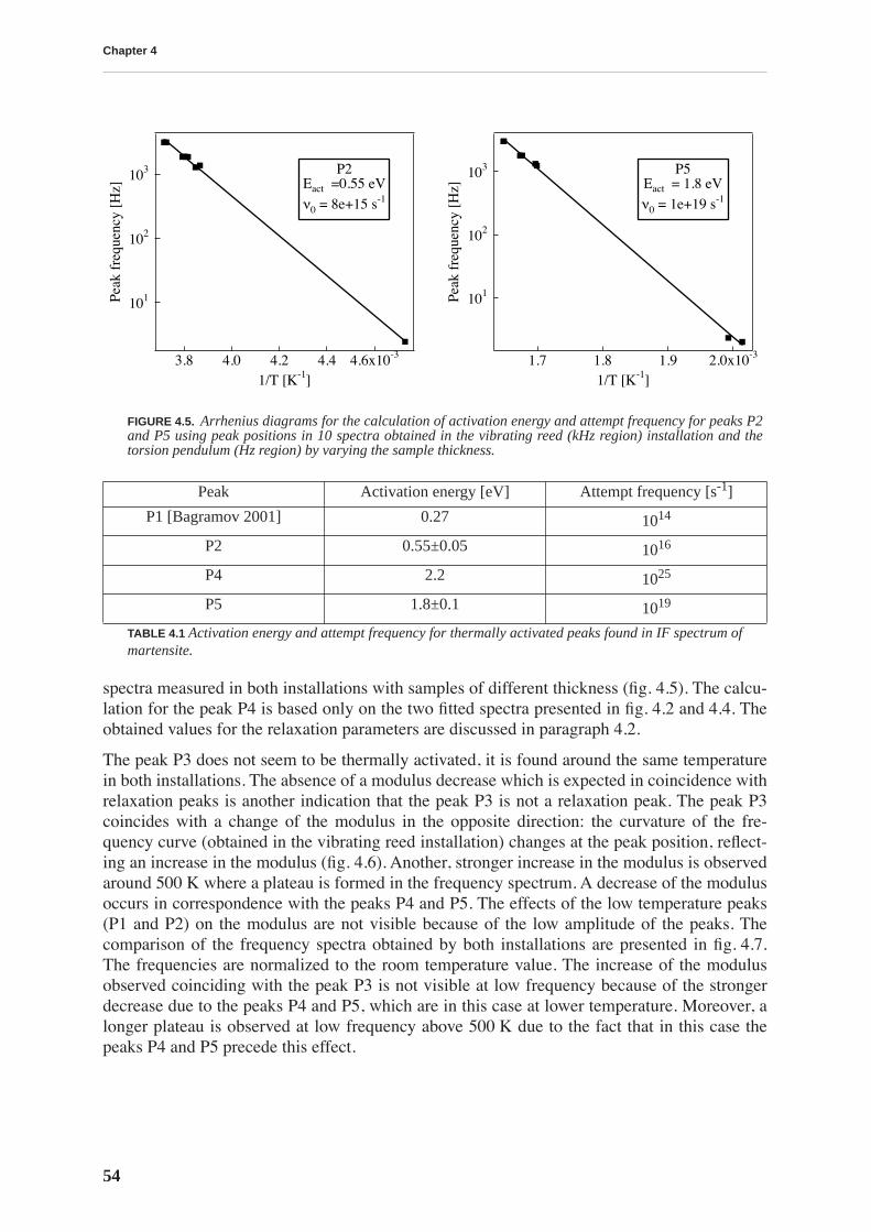
Chapter 4
54
spectra measured in both installations with samples of different thickness (fig. 4.5). The calcu-lation for the peak P4 is based only on the two fitted spectra presented in fig. 4.2 and 4.4. Theobtained values for the relaxation parameters are discussed in paragraph 4.2.
The peak P3 does not seem to be thermally activated, it is found around the same temperaturein both installations. The absence of a modulus decrease which is expected in coincidence withrelaxation peaks is another indication that the peak P3 is not a relaxation peak. The peak P3coincides with a change of the modulus in the opposite direction: the curvature of the fre-quency curve (obtained in the vibrating reed installation) changes at the peak position, reflect-ing an increase in the modulus (fig. 4.6). Another, stronger increase in the modulus is observedaround 500 K where a plateau is formed in the frequency spectrum. A decrease of the modulusoccurs in correspondence with the peaks P4 and P5. The effects of the low temperature peaks(P1 and P2) on the modulus are not visible because of the low amplitude of the peaks. Thecomparison of the frequency spectra obtained by both installations are presented in fig. 4.7.The frequencies are normalized to the room temperature value. The increase of the modulusobserved coinciding with the peak P3 is not visible at low frequency because of the strongerdecrease due to the peaks P4 and P5, which are in this case at lower temperature. Moreover, alonger plateau is observed at low frequency above 500 K due to the fact that in this case thepeaks P4 and P5 precede this effect.
FIGURE 4.5.
Arrhenius diagrams for the calculation of activation energy and attempt frequency for peaks P2and P5 using peak positions in 10 spectra obtained in the vibrating reed (kHz region) installation and thetorsion pendulum (Hz region) by varying the sample thickness.
Peak Activation energy [eV] Attempt frequency [s
-1
]
P1 [Bagramov 2001] 0.27 10
14
P2 0.55±0.05 10
16
P4 2.2 10
25
P5 1.8±0.1 10
19
TABLE 4.1
Activation energy and attempt frequency for thermally activated peaks found in IF spectrum of martensite.
101
102
103
Peak
fre
quen
cy [
Hz]
4.6x10-34.44.24.03.81/T [K-1]
P2Eact =0.55 eV
ν0 = 8e+15 s-1
101
102
103
Peak
fre
quen
cy [
Hz]
2.0x10-31.91.81.71/T [K-1]
P5Eact = 1.8 eV
ν0 = 1e+19 s-1
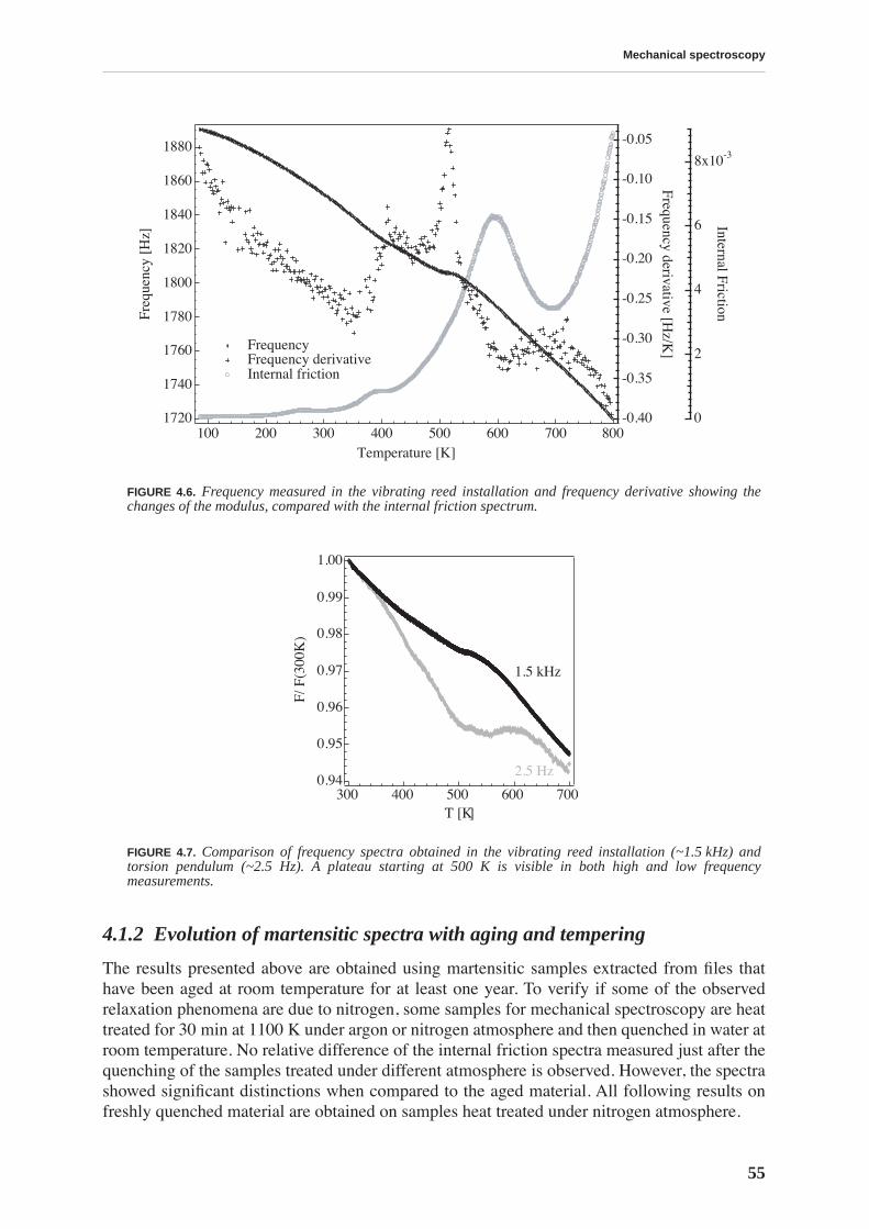
Mechanical spectroscopy
55
4.1.2 Evolution of martensitic spectra with aging and tempering
The results presented above are obtained using martensitic samples extracted from files thathave been aged at room temperature for at least one year. To verify if some of the observedrelaxation phenomena are due to nitrogen, some samples for mechanical spectroscopy are heattreated for 30 min at 1100 K under argon or nitrogen atmosphere and then quenched in water atroom temperature. No relative difference of the internal friction spectra measured just after thequenching of the samples treated under different atmosphere is observed. However, the spectrashowed significant distinctions when compared to the aged material. All following results onfreshly quenched material are obtained on samples heat treated under nitrogen atmosphere.
FIGURE 4.6.
Frequency measured in the vibrating reed installation and frequency derivative showing thechanges of the modulus, compared with the internal friction spectrum.
FIGURE 4.7.
Comparison of frequency spectra obtained in the vibrating reed installation (~1.5 kHz) andtorsion pendulum (~2.5 Hz). A plateau starting at 500 K is visible in both high and low frequencymeasurements.
8x10⁻³
6
4
2
0
Internal Friction
800700600500400300200100Temperature [K]
1880
1860
1840
1820
1800
1780
1760
1740
1720
Freq
uenc
y [H
z]
-0.40
-0.35
-0.30
-0.25
-0.20
-0.15
-0.10
-0.05
Frequency derivative [Hz/K
] Frequency Frequency derivative Internal friction
1.00
0.99
0.98
0.97
0.96
0.95
0.94
F/ F
(300
K)
700600500400300T [K]
2.5 Hz
1.5 kHz
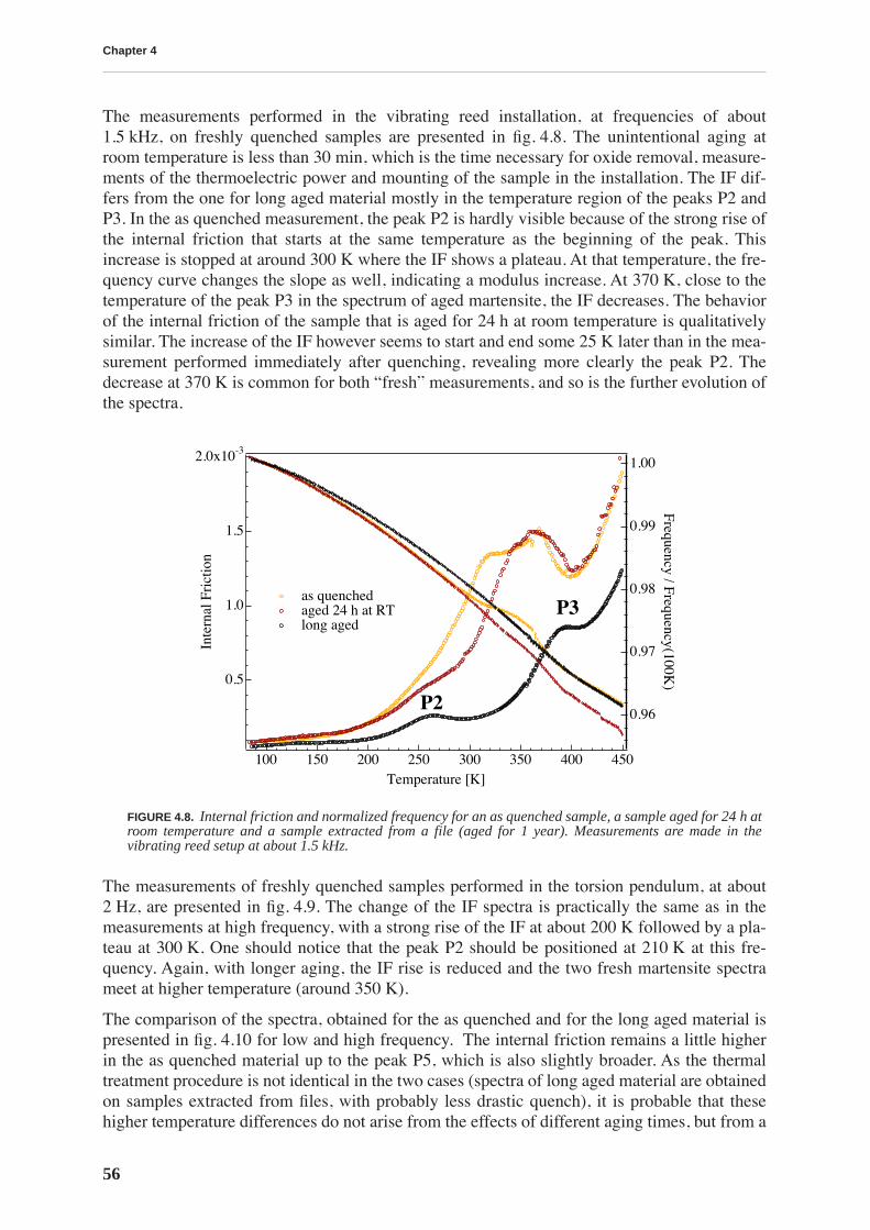
Chapter 4
56
The measurements performed in the vibrating reed installation, at frequencies of about1.5 kHz, on freshly quenched samples are presented in fig. 4.8. The unintentional aging atroom temperature is less than 30 min, which is the time necessary for oxide removal, measure-ments of the thermoelectric power and mounting of the sample in the installation. The IF dif-fers from the one for long aged material mostly in the temperature region of the peaks P2 andP3. In the as quenched measurement, the peak P2 is hardly visible because of the strong rise ofthe internal friction that starts at the same temperature as the beginning of the peak. Thisincrease is stopped at around 300 K where the IF shows a plateau. At that temperature, the fre-quency curve changes the slope as well, indicating a modulus increase. At 370 K, close to thetemperature of the peak P3 in the spectrum of aged martensite, the IF decreases. The behaviorof the internal friction of the sample that is aged for 24 h at room temperature is qualitativelysimilar. The increase of the IF however seems to start and end some 25 K later than in the mea-surement performed immediately after quenching, revealing more clearly the peak P2. Thedecrease at 370 K is common for both “fresh” measurements, and so is the further evolution ofthe spectra.
The measurements of freshly quenched samples performed in the torsion pendulum, at about2 Hz, are presented in fig. 4.9. The change of the IF spectra is practically the same as in themeasurements at high frequency, with a strong rise of the IF at about 200 K followed by a pla-teau at 300 K. One should notice that the peak P2 should be positioned at 210 K at this fre-quency. Again, with longer aging, the IF rise is reduced and the two fresh martensite spectrameet at higher temperature (around 350 K).
The comparison of the spectra, obtained for the as quenched and for the long aged material ispresented in fig. 4.10 for low and high frequency. The internal friction remains a little higherin the as quenched material up to the peak P5, which is also slightly broader. As the thermaltreatment procedure is not identical in the two cases (spectra of long aged material are obtainedon samples extracted from files, with probably less drastic quench), it is probable that thesehigher temperature differences do not arise from the effects of different aging times, but from a
FIGURE 4.8.
Internal friction and normalized frequency for an as quenched sample, a sample aged for 24 h atroom temperature and a sample extracted from a file (aged for 1 year). Measurements are made in thevibrating reed setup at about 1.5 kHz.
2.0x10⁻³
1.5
1.0
0.5
Inte
rnal
Fri
ctio
n
450400350300250200150100Temperature [K]
1.00
0.99
0.98
0.97
0.96
Frequency / Frequency(100K)
as quenched aged 24 h at RT long aged
P2
P3

Mechanical spectroscopy
57
slightly modified structure of the material (for example dislocation density, fraction of platemartensite etc.).
The differences at low temperature in IF spectra between long aged and freshly quenched sam-ples are obviously due to the different aging time. One hour tempering at 375 K of a sampleaged for 2 days at room temperature, which still shows a strong IF increase at 250 K, reducesthe IF to the level of the long aged specimen (fig. 4.11).
FIGURE 4.9.
Internal friction for a sample aged for 2 h at room temperature, a sample aged for 48 h at roomtemperature and a sample extracted from a file (aged for 1 year). Measurements are made in the torsionpendulum at about 2 Hz.
FIGURE 4.10.
As quenched compared to long aged material internal friction spectra, as measured in thevibrating reed installation (about 1.5 kHz, crosses) and the torsion pendulum (about 2 Hz, circles).
6x10⁻³
4
2
0
Inte
rnal
fri
ctio
n
450400350300250200150100Temperature [K]
aged 2h at RT aged 48h at RT long aged
P2P3
12x10-3
10
8
6
4
2
0
Inte
rnal
fri
ctio
n
800700600500400300200100Temperature [K]
2 Hz aged 2h at RT long aged
1.5 kHz
as quenched long aged
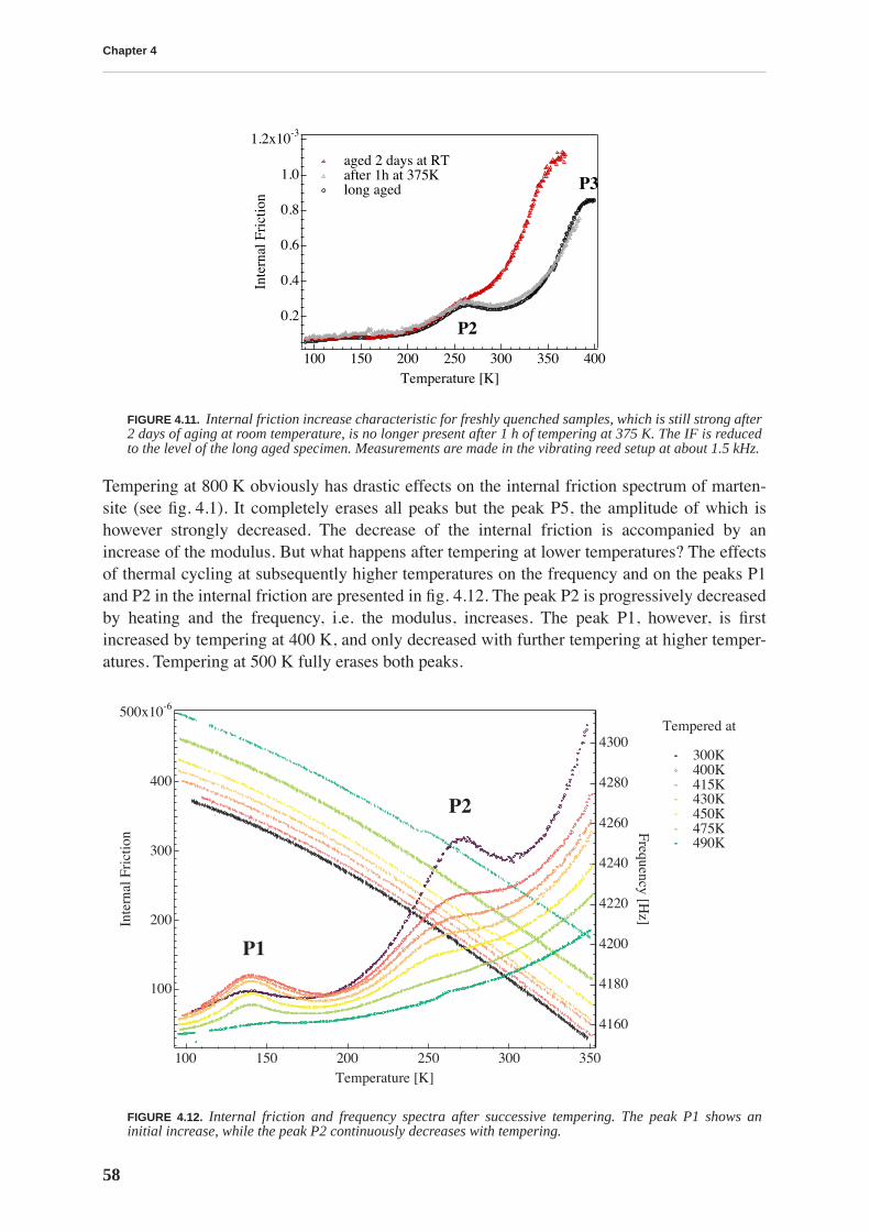
Chapter 4
58
Tempering at 800 K obviously has drastic effects on the internal friction spectrum of marten-site (see fig. 4.1). It completely erases all peaks but the peak P5, the amplitude of which ishowever strongly decreased. The decrease of the internal friction is accompanied by anincrease of the modulus. But what happens after tempering at lower temperatures? The effectsof thermal cycling at subsequently higher temperatures on the frequency and on the peaks P1and P2 in the internal friction are presented in fig. 4.12. The peak P2 is progressively decreasedby heating and the frequency, i.e. the modulus, increases. The peak P1, however, is firstincreased by tempering at 400 K, and only decreased with further tempering at higher temper-atures. Tempering at 500 K fully erases both peaks.
FIGURE 4.11.
Internal friction increase characteristic for freshly quenched samples, which is still strong after2 days of aging at room temperature, is no longer present after 1 h of tempering at 375 K. The IF is reducedto the level of the long aged specimen. Measurements are made in the vibrating reed setup at about 1.5 kHz.
FIGURE 4.12.
Internal friction and frequency spectra after successive tempering. The peak P1 shows aninitial increase, while the peak P2 continuously decreases with tempering.
1.2x10⁻³
1.0
0.8
0.6
0.4
0.2
Inte
rnal
Fri
ctio
n
400350300250200150100Temperature [K]
aged 2 days at RT after 1h at 375K long aged
P2
P3
4300
4280
4260
4240
4220
4200
4180
4160
Frequency [Hz]
350300250200150100Temperature [K]
500x10-6
400
300
200
100
Inte
rnal
Fri
ctio
n
Tempered at
300K 400K 415K 430K 450K 475K 490K
P1
P2
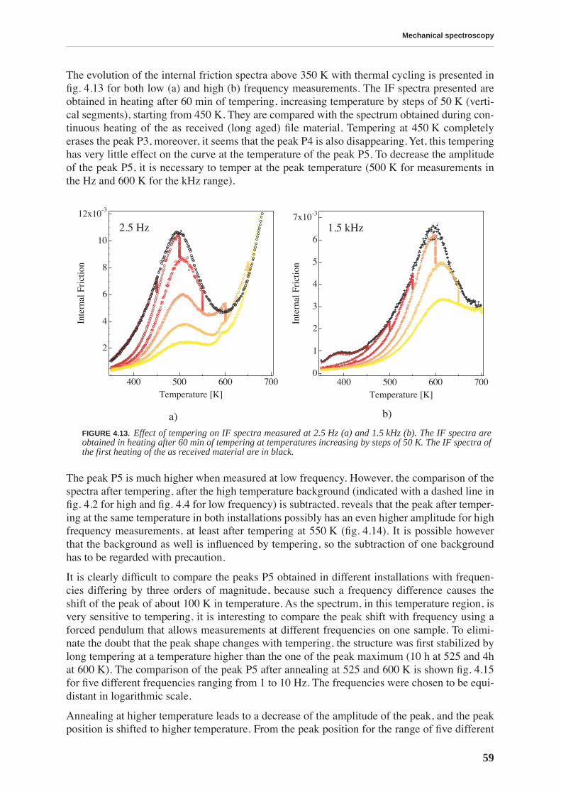
Mechanical spectroscopy
59
The evolution of the internal friction spectra above 350 K with thermal cycling is presented infig. 4.13 for both low (a) and high (b) frequency measurements. The IF spectra presented areobtained in heating after 60 min of tempering, increasing temperature by steps of 50 K (verti-cal segments), starting from 450 K. They are compared with the spectrum obtained during con-tinuous heating of the as received (long aged) file material. Tempering at 450 K completelyerases the peak P3, moreover, it seems that the peak P4 is also disappearing. Yet, this temperinghas very little effect on the curve at the temperature of the peak P5. To decrease the amplitudeof the peak P5, it is necessary to temper at the peak temperature (500 K for measurements inthe Hz and 600 K for the kHz range).
The peak P5 is much higher when measured at low frequency. However, the comparison of thespectra after tempering, after the high temperature background (indicated with a dashed line infig. 4.2 for high and fig. 4.4 for low frequency) is subtracted, reveals that the peak after temper-ing at the same temperature in both installations possibly has an even higher amplitude for highfrequency measurements, at least after tempering at 550 K (fig. 4.14). It is possible howeverthat the background as well is influenced by tempering, so the subtraction of one backgroundhas to be regarded with precaution.
It is clearly difficult to compare the peaks P5 obtained in different installations with frequen-cies differing by three orders of magnitude, because such a frequency difference causes theshift of the peak of about 100 K in temperature. As the spectrum, in this temperature region, isvery sensitive to tempering, it is interesting to compare the peak shift with frequency using aforced pendulum that allows measurements at different frequencies on one sample. To elimi-nate the doubt that the peak shape changes with tempering, the structure was first stabilized bylong tempering at a temperature higher than the one of the peak maximum (10 h at 525 and 4hat 600 K). The comparison of the peak P5 after annealing at 525 and 600 K is shown fig. 4.15for five different frequencies ranging from 1 to 10 Hz. The frequencies were chosen to be equi-distant in logarithmic scale.
Annealing at higher temperature leads to a decrease of the amplitude of the peak, and the peakposition is shifted to higher temperature. From the peak position for the range of five different
a) b)
FIGURE 4.13.
Effect of tempering on IF spectra measured at 2.5 Hz (a) and 1.5 kHz (b). The IF spectra areobtained in heating after 60 min of tempering at temperatures increasing by steps of 50 K. The IF spectra ofthe first heating of the as received material are in black.
12x10-3
10
8
6
4
2
Inte
rnal
Fri
ctio
n
700600500400Temperature [K]
2.5 Hz7x10-3
6
5
4
3
2
1
0
Inte
rnal
Fri
ctio
n
700600500400Temperature [K]
1.5 kHz
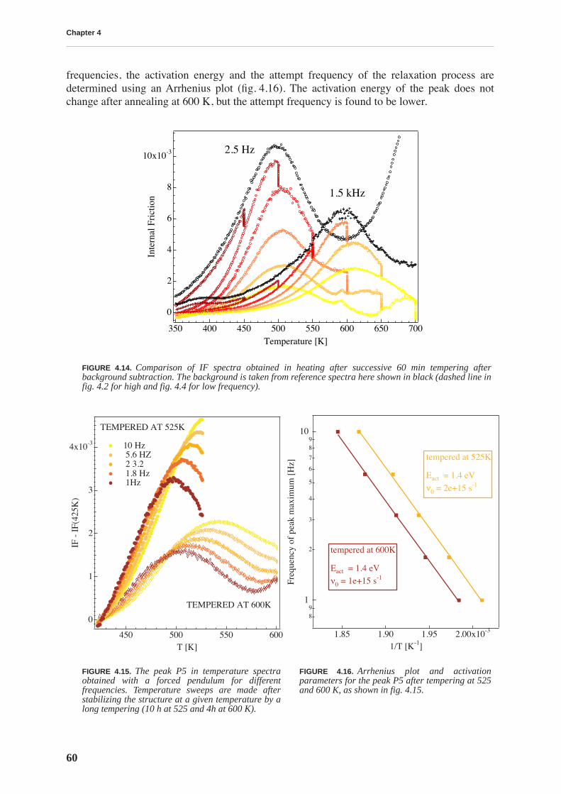
Chapter 4
60
frequencies, the activation energy and the attempt frequency of the relaxation process aredetermined using an Arrhenius plot (fig. 4.16). The activation energy of the peak does notchange after annealing at 600 K, but the attempt frequency is found to be lower.
FIGURE 4.14.
Comparison of IF spectra obtained in heating after successive 60 min tempering afterbackground subtraction. The background is taken from reference spectra here shown in black (dashed line infig. 4.2 for high and fig. 4.4 for low frequency).
FIGURE 4.15.
The peak P5 in temperature spectraobtained with a forced pendulum for differentfrequencies. Temperature sweeps are made afterstabilizing the structure at a given temperature by along tempering (10 h at 525 and 4h at 600 K).
FIGURE 4.16.
Arrhenius plot and activationparameters for the peak P5 after tempering at 525and 600 K, as shown in fig. 4.15.
10x10-3
8
6
4
2
0
Inte
rnal
Fri
ctio
n
700650600550500450400350Temperature [K]
2.5 Hz
1.5 kHz
4x10⁻³
3
2
1
0
IF -
IF(
425K
)
600550500450T [K]
TEMPERED AT 525K
10 Hz 5.6 HZ 2 3.2 1.8 Hz 1Hz
TEMPERED AT 600K 8
91
2
3
4
5
6
7
89
10
Freq
uenc
y of
pea
k m
axim
um [
Hz]
2.00x10-31.951.901.851/T [K-1]
tempered at 525K Eact = 1.4 eVν0 = 2e+15 s-1
tempered at 600K Eact = 1.4 eVν0 = 1e+15 s-1
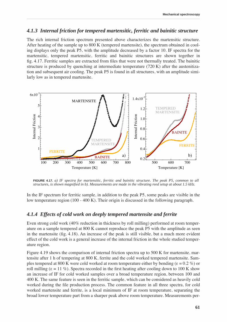
Mechanical spectroscopy
61
4.1.3 Internal friction for tempered martensitic, ferritic and bainitic structure
The rich internal friction spectrum presented above characterizes the martensitic structure.After heating of the sample up to 800 K (tempered martensite), the spectrum obtained in cool-ing displays only the peak P5, with the amplitude decreased by a factor 10. IF spectra for themartensitic, tempered martensitic, ferritic and bainitic structures are shown together infig. 4.17. Ferritic samples are extracted from files that were not thermally treated. The bainiticstructure is produced by quenching at intermediate temperature (720 K) after the austenitiza-tion and subsequent air cooling. The peak P5 is found in all structures, with an amplitude simi-larly low as in tempered martensite.
In the IF spectrum for ferritic sample, in addition to the peak P5, some peaks are visible in thelow temperature region (100 - 400 K). Their origin is discussed in the following paragraph.
4.1.4 Effects of cold work on deeply tempered martensite and ferrite
Even strong cold work (40% reduction in thickness by roll milling) performed at room temper-ature on a sample tempered at 800 K cannot reproduce the peak P5 with the amplitude as seenin the martensite (fig. 4.18). An increase of the peak is still visible, but a much more evidenteffect of the cold work is a general increase of the internal friction in the whole studied temper-ature region.
Figure 4.19 shows the comparison of internal friction spectra up to 500 K for martensite, mar-tensite after 1 h of tempering at 800 K, ferrite and the cold worked tempered martensite. Sam-ples tempered at 800 K were cold worked at room temperature either by bending (
ε
= 0.2 %) orroll milling (
ε
= 11 %). Spectra recorded in the first heating after cooling down to 100 K showan increase of IF for cold worked samples over a broad temperature region, between 100 and400 K. The same feature is seen in the ferritic sample, which can be considered as heavily coldworked during the file production process. The common feature in all three spectra, for coldworked martensite and ferrite, is a local minimum of IF at room temperature, separating thebroad lower temperature part from a sharper peak above room temperature. Measurements per-
FIGURE 4.17.
a) IF spectra for martensitic, ferritic and bainitic structure. The peak P5, common to allstructures, is shown magnified in b). Measurements are made in the vibrating reed setup at about 1.5 kHz.
a) b)
1.4x10⁻³
1.2
1.0
0.8
0.6
0.4
0.2
Inte
rnal
Fri
ctio
n
700600500Temperature [K]
TEMPERED MARTENSITE
BAINITE
FERRITE
6x10⁻³
5
4
3
2
1
Inte
rnal
Fri
ctio
n
800700600500400300200100Temperature [K]
TEMPEREDMARTENSITE
BAINITE
FERRITE
MARTENSITE
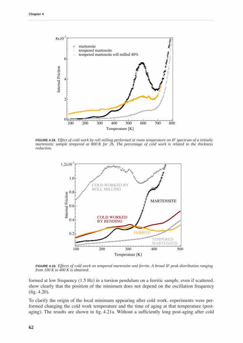
Chapter 4
62
formed at low frequency (1.5 Hz) in a torsion pendulum on a ferritic sample, even if scattered,show clearly that the position of the minimum does not depend on the oscillation frequency(fig. 4.20).
To clarify the origin of the local minimum appearing after cold work, experiments were per-formed changing the cold work temperature and the time of aging at that temperature (post-aging). The results are shown in fig. 4.21a. Without a sufficiently long post-aging after cold
FIGURE 4.18.
Effect of cold work by roll milling performed at room temperature on IF spectrum of a initiallymartensitic sample tempered at 800 K for 2h. The percentage of cold work is related to the thicknessreduction.
FIGURE 4.19.
Effects of cold work on tempered martensite and ferrite. A broad IF peak distribution rangingfrom 100 K to 400 K is obtained.
8x10⁻³
6
4
2
0
Inte
rnal
Fri
ctio
n
800700600500400300200100Temperature [K]
martensite tempered martensite tempered martensite roll milled 40%
1.2x10⁻³
1.0
0.8
0.6
0.4
0.2
Inte
rnal
Fri
ctio
n
500400300200100Temperature [K]
COLD WORKED BY ROLL MILLING
COLD WORKEDBY BENDING
FERRITE
MARTENSITE
TEMPEREDMARTENSITE
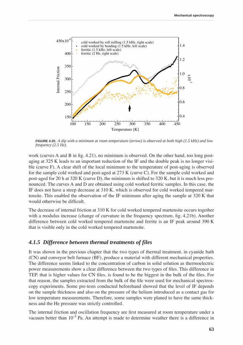
Mechanical spectroscopy
63
work (curves A and B in fig. 4.21), no minimum is observed. On the other hand, too long post-aging at 325 K leads to an important reduction of the IF and the double peak is no longer visi-ble (curve F). A clear shift of the local minimum to the temperature of post-aging is observedfor the sample cold worked and post-aged at 273 K (curve C). For the sample cold worked andpost-aged for 20 h at 320 K (curve D), the minimum is shifted to 320 K, but it is much less pro-nounced. The curves A and D are obtained using cold worked ferritic samples. In this case, theIF does not have a steep decrease at 310 K, which is observed for cold worked tempered mar-tensite. This enabled the observation of the IF minimum after aging the sample at 320 K thatwould otherwise be difficult.
The decrease of internal friction at 310 K for cold worked tempered martensite occurs togetherwith a modulus increase (change of curvature in the frequency spectrum, fig. 4.21b). Anotherdifference between cold worked tempered martensite and ferrite is an IF peak around 390 Kthat is visible only in the cold worked tempered martensite.
4.1.5 Difference between thermal treatments of files
It was shown in the previous chapter that the two types of thermal treatment, in cyanide bath(CN) and conveyor belt furnace (BF), produce a material with different mechanical properties.The difference seems linked to the concentration of carbon in solid solution as thermoelectricpower measurements show a clear difference between the two types of files. This difference inTEP, that is higher values for CN files, is found to be the biggest in the bulk of the files. Forthat reason, the samples extracted from the bulk of the file were used for mechanical spectros-copy experiments. Some pre-tests conducted beforehand showed that the level of IF dependson the sample thickness and also on the pressure of the helium introduced as a contact gas forlow temperature measurements. Therefore, some samples were planed to have the same thick-ness and the He pressure was strictly controlled.
The internal friction and oscillation frequency are first measured at room temperature under avacuum better than 10
-3
Pa. An attempt is made to determine weather there is a difference in
FIGURE 4.20.
A dip with a minimum at room temperature (arrow) is observed at both high (1.5 kHz) and lowfrequency (2.5 Hz).
1.4
1.2
1.0
0.8
0.6
0.4
x10-3
450400350300250200150100Temperature [K]
450x10-6
400
350
300
250
200
150
Inte
rnal
Fri
ctio
n
cold worked by roll milling (1.5 kHz, right scale) cold worked by bending (1.5 kHz, left scale) ferritic (1.5 kHz, left scale) ferritic (2 Hz, right scale)
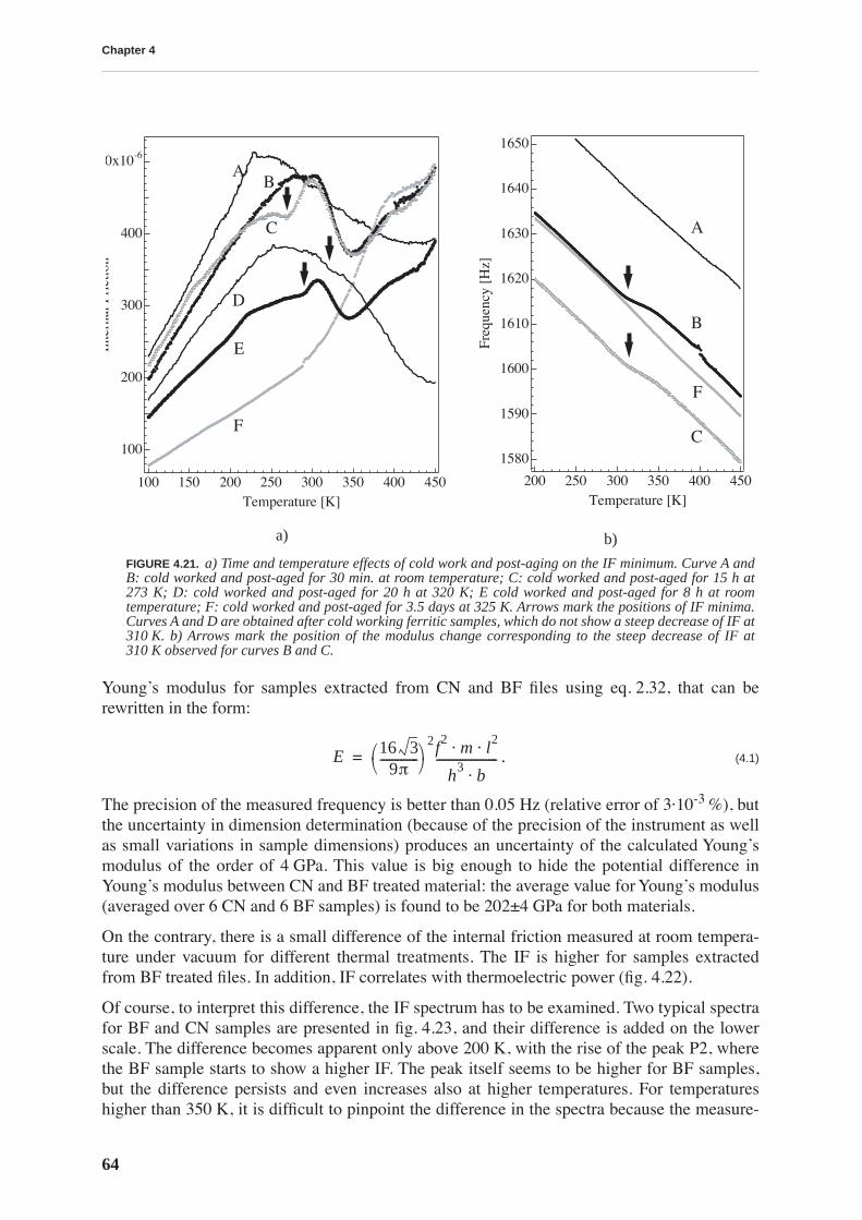
Chapter 4
64
Young’s modulus for samples extracted from CN and BF files using eq. 2.32, that can berewritten in the form:
.
(4.1)
The precision of the measured frequency is better than 0.05 Hz (relative error of 3·10
-3
%), butthe uncertainty in dimension determination (because of the precision of the instrument as wellas small variations in sample dimensions) produces an uncertainty of the calculated Young’smodulus of the order of 4 GPa. This value is big enough to hide the potential difference inYoung’s modulus between CN and BF treated material: the average value for Young’s modulus(averaged over 6 CN and 6 BF samples) is found to be 202±4 GPa for both materials.
On the contrary, there is a small difference of the internal friction measured at room tempera-ture under vacuum for different thermal treatments. The IF is higher for samples extractedfrom BF treated files. In addition, IF correlates with thermoelectric power (fig. 4.22).
Of course, to interpret this difference, the IF spectrum has to be examined. Two typical spectrafor BF and CN samples are presented in fig. 4.23, and their difference is added on the lowerscale. The difference becomes apparent only above 200 K, with the rise of the peak P2, wherethe BF sample starts to show a higher IF. The peak itself seems to be higher for BF samples,but the difference persists and even increases also at higher temperatures. For temperatureshigher than 350 K, it is difficult to pinpoint the difference in the spectra because the measure-
a) b)
FIGURE 4.21.
a) Time and temperature effects of cold work and post-aging on the IF minimum. Curve A andB: cold worked and post-aged for 30 min. at room temperature; C: cold worked and post-aged for 15 h at273 K; D: cold worked and post-aged for 20 h at 320 K; E cold worked and post-aged for 8 h at roomtemperature; F: cold worked and post-aged for 3.5 days at 325 K. Arrows mark the positions of IF minima.Curves A and D are obtained after cold working ferritic samples, which do not show a steep decrease of IF at310 K. b) Arrows mark the position of the modulus change corresponding to the steep decrease of IF at310 K observed for curves B and C.
0x10-6
400
300
200
100
Inte
rnal
Fri
ctio
n
450400350300250200150100Temperature [K]
B
C
D
E
F
A
1650
1640
1630
1620
1610
1600
1590
1580
Freq
uenc
y [H
z]450400350300250200
Temperature [K]
B
C
F
A
E 16 39π
-------------⎝ ⎠⎛ ⎞
2f2 m l2⋅ ⋅
h3 b⋅---------------------=
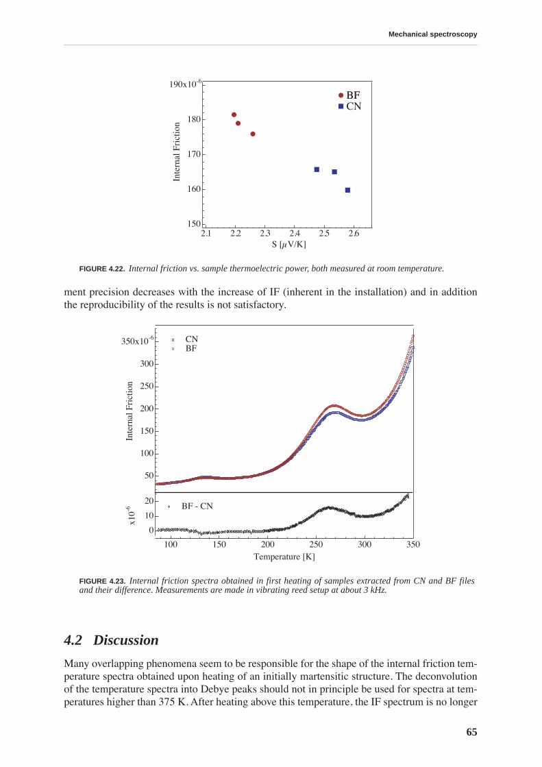
Mechanical spectroscopy
65
ment precision decreases with the increase of IF (inherent in the installation) and in additionthe reproducibility of the results is not satisfactory.
4.2 Discussion
Many overlapping phenomena seem to be responsible for the shape of the internal friction tem-perature spectra obtained upon heating of an initially martensitic structure. The deconvolutionof the temperature spectra into Debye peaks should not in principle be used for spectra at tem-peratures higher than 375 K. After heating above this temperature, the IF spectrum is no longer
FIGURE 4.22.
Internal friction vs. sample thermoelectric power, both measured at room temperature.
FIGURE 4.23.
Internal friction spectra obtained in first heating of samples extracted from CN and BF filesand their difference. Measurements are made in vibrating reed setup at about 3 kHz.
190x10-6
180
170
160
150
Inte
rnal
Fri
ctio
n
2.62.52.42.32.22.1S [µV/K]
BFBFCN
350x10-6
300
250
200
150
100
50
Inte
rnal
Fri
ctio
n
350300250200150100Temperature [K]
20
10
0
x10-6
CN BF
BF - CN
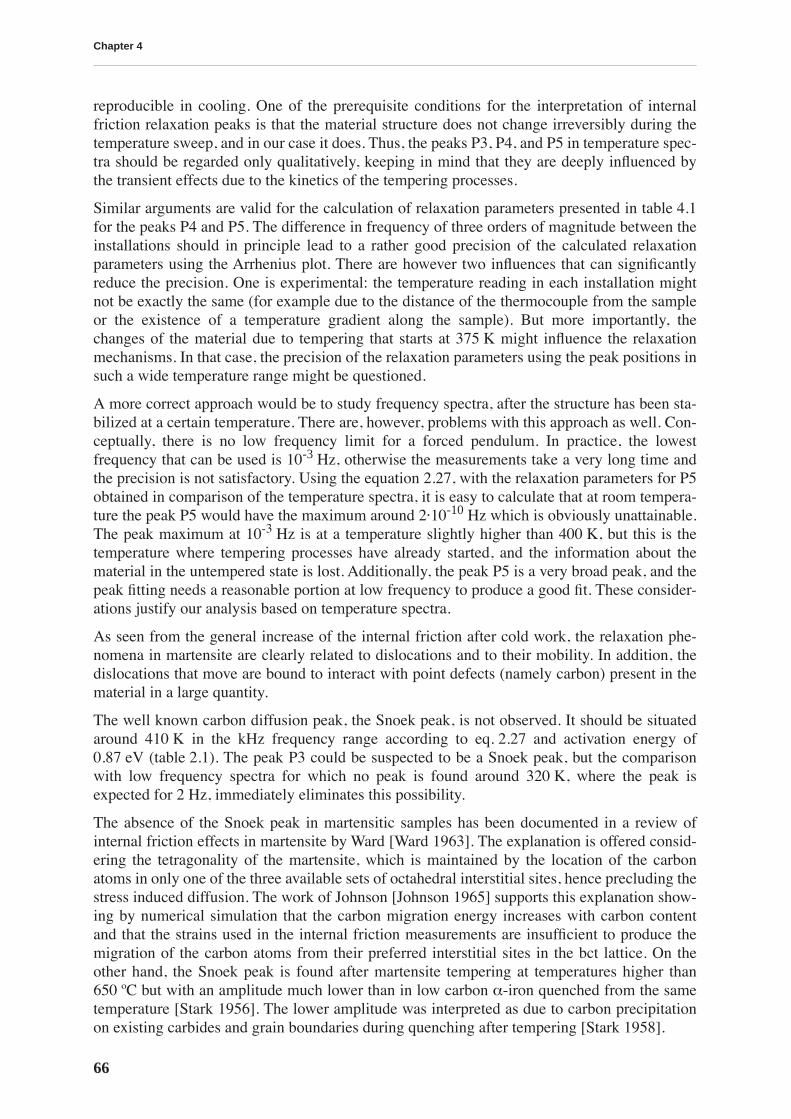
Chapter 4
66
reproducible in cooling. One of the prerequisite conditions for the interpretation of internalfriction relaxation peaks is that the material structure does not change irreversibly during thetemperature sweep, and in our case it does. Thus, the peaks P3, P4, and P5 in temperature spec-tra should be regarded only qualitatively, keeping in mind that they are deeply influenced bythe transient effects due to the kinetics of the tempering processes.
Similar arguments are valid for the calculation of relaxation parameters presented in table 4.1for the peaks P4 and P5. The difference in frequency of three orders of magnitude between theinstallations should in principle lead to a rather good precision of the calculated relaxationparameters using the Arrhenius plot. There are however two influences that can significantlyreduce the precision. One is experimental: the temperature reading in each installation mightnot be exactly the same (for example due to the distance of the thermocouple from the sampleor the existence of a temperature gradient along the sample). But more importantly, thechanges of the material due to tempering that starts at 375 K might influence the relaxationmechanisms. In that case, the precision of the relaxation parameters using the peak positions insuch a wide temperature range might be questioned.
A more correct approach would be to study frequency spectra, after the structure has been sta-bilized at a certain temperature. There are, however, problems with this approach as well. Con-ceptually, there is no low frequency limit for a forced pendulum. In practice, the lowestfrequency that can be used is 10
-3
Hz, otherwise the measurements take a very long time andthe precision is not satisfactory. Using the equation 2.27, with the relaxation parameters for P5obtained in comparison of the temperature spectra, it is easy to calculate that at room tempera-ture the peak P5 would have the maximum around 2·10
-10
Hz which is obviously unattainable.The peak maximum at 10
-3
Hz is at a temperature slightly higher than 400 K, but this is thetemperature where tempering processes have already started, and the information about thematerial in the untempered state is lost. Additionally, the peak P5 is a very broad peak, and thepeak fitting needs a reasonable portion at low frequency to produce a good fit. These consider-ations justify our analysis based on temperature spectra.
As seen from the general increase of the internal friction after cold work, the relaxation phe-nomena in martensite are clearly related to dislocations and to their mobility. In addition, thedislocations that move are bound to interact with point defects (namely carbon) present in thematerial in a large quantity.
The well known carbon diffusion peak, the Snoek peak, is not observed. It should be situatedaround 410 K in the kHz frequency range according to eq. 2.27 and activation energy of0.87 eV (table 2.1). The peak P3 could be suspected to be a Snoek peak, but the comparisonwith low frequency spectra for which no peak is found around 320 K, where the peak isexpected for 2 Hz, immediately eliminates this possibility.
The absence of the Snoek peak in martensitic samples has been documented in a review ofinternal friction effects in martensite by Ward [Ward 1963]. The explanation is offered consid-ering the tetragonality of the martensite, which is maintained by the location of the carbonatoms in only one of the three available sets of octahedral interstitial sites, hence precluding thestress induced diffusion. The work of Johnson [Johnson 1965] supports this explanation show-ing by numerical simulation that the carbon migration energy increases with carbon contentand that the strains used in the internal friction measurements are insufficient to produce themigration of the carbon atoms from their preferred interstitial sites in the bct lattice. On theother hand, the Snoek peak is found after martensite tempering at temperatures higher than650 ºC but with an amplitude much lower than in low carbon
α
-iron quenched from the sametemperature [Stark 1956]. The lower amplitude was interpreted as due to carbon precipitationon existing carbides and grain boundaries during quenching after tempering [Stark 1958].

Mechanical spectroscopy
67
The absence of the Snoek peak is therefore not surprising for the martensite, but its absence inthe tempered martensite or ferrite is more intriguing. It can be concluded that although somecarbon is still present in solid solution (justified by the existence of the peak P5 in these struc-tures, which is, as shown below, interpreted as Snoek-Köster carbon peak), the carbon atomsare not free to move from one type of octahedral site to the other under the applied cyclicstress. The residual tetragonality of tempered martensite could not explain the absence of thepeak in ferrite. The reason why the Snoek peak is never observed could be that most of the car-bon precipitates during cooling and the remaining carbon atoms are bound to dislocationsor/and to other impurities.
The decrease of the Snoek peak in steels with addition of substitutionals, such as Co, Mn, Cr,Si, P and Al, has been evidenced for low impurity concentrations [Numakura 1996, Saitoh2004, Massardier 2004]. The strain field generated by a substitutional atom due to the differ-ence in atomic size is concluded to be the main reason for the reduction in Snoek peak height.As our steel contains 0.34 wt. % of Mn and 0.22 wt. % of Si as well as some other impurities,it is possible that they affect the carbon mobility.
If carbon atoms are bound to dislocations after tempering, they might be freed from them bycold work. It might be argued that the peak observed around 390 K in cold worked temperedmartensite is a Snoek peak. However, this hypothesis is not confirmed by a modulus defect infrequency spectra nor by measurements at low frequency. Therefore it is more likely that thepeak is due to a mechanism comparable to the one that causes the peak P3 in the IF spectrumof martensite.
P1
The peak P1 is observed around 130 K in the high frequency measurements and thus it may beinterpreted as Snoek-Köster hydrogen peak according to literature. In previous measurementson this material [Bagramov 2001], the peak was detected also in the low frequency spectrumobtained in torsion (fig. 2.21b). From the temperature of the peak for low and high frequency(99.1 K at 1 Hz and 132.6 K at 3.1 Hz), the activation energy of the peak is calculated to be0.27 eV, comparing reasonably well to the 0.22±0.1 eV found by San Juan et al. in pure iron[San Juan 1985]. As the peak is also sensitive to cold work (fig. 2.21b), it is attributed to arelaxation of Snoek-Köster type involving non-screw dislocations and hydrogen atoms.
An interesting characteristic feature of the peak P1 is its evolution during tempering. Contraryto the behavior of other peaks, for which tempering leads to a reduction of the amplitude, theamplitude of the peak P1 is initially increased by tempering (fig. 4.12). For tempering at tem-peratures higher than 400 K, the amplitude of the peak decreases, and after tempering at tem-peratures higher than 500 K the peak disappears. The increase of the peak is also observedafter aging the samples at room temperature. Moreover, the peak is hardly visible for asquenched material (fig. 4.8).
The increase of the amplitude of the peak P1 observed after tempering at 400 K could be justi-fied by carbon precipitation. For a dragging mechanism (dislocation segments dragging pointdefects), the amplitude of a relaxation peak is proportional to , the square of the average dis-location length between the strong pinning points (eq. 2.35). At the temperature of the peak P1,which is around 140 K, soluted carbon atoms can be considered as immobile and thereforeplaying the role of strong pinners. Precipitation of carbon in form of carbides during temperingmay decrease the amount of the carbon segregated on the dislocations, therefore leading to anincrease of with a consequent increase of the peak amplitude. The position of the peakshould also be influenced by through the attempt frequency
ν
0
(eq. 2.36). But, using theparameters of the peak listed in table 4.1, it can be calculated that an increase of of 50 %
L2
L2
L2
L2
Chapter 4
68
would cause a shift of the peak to higher temperature of only 3 K. The decrease of the peak byfurther tempering (for temperatures higher than 450 K) could be caused by a decrease of thedislocation mobility by pinning with precipitates, and for higher temperatures by a decrease ofthe dislocation density combined with the degassing of hydrogen from the material.
P5
The most striking feature of the IF spectrum of the martensite is the peak P5 due to its ampli-tude, which is notably higher than the amplitudes of the other peaks. It is also the only peakthat can be found in bainitic and ferritic (tempered martensitic) structures, though having amuch smaller amplitude. The peak temperature (for a given frequency) and amplitude corre-sponds to the Snoek-Köster peak regularly found in iron-carbon martensite and cold workedferrite containing interstitial impurities (see for example [Ward 1963, Petarra 1967, Klems1976]). The Snoek-Köster peak is related to the dragging of carbon atoms by kink pairs form-ing on screw dislocations [Seeger 1979] (see section 2.5).
The relaxation parameters of the peak can be determined by comparing the measurements intorsion and bending, which are three orders of magnitude apart in frequency. The Arrheniusplot presented in fig. 4.5 gives a value for the activation enthalpy H = 1.8±0.1 eV with theattempt frequency
ν
0=1019 s-1. The value for the activation energy fits in the range of energiesmeasured by other authors for the Snoek-Köster relaxation peak in α-iron and carbon steelmartensite of 1.4 to 1.9 eV [Klems 1976]. It can be interpreted (see page 30) as the sum of theenergy for kink pair formation on screw dislocations, 2Hk = 0.94 eV [Schultz 1991], and theenergy for carbon diffusion, HS = 0.87 eV (table 2.1). However, the attempt frequency is (asalso found by other authors) too high to be physical. The attempt frequency for a relaxationdue to point defects is expected to be of the order of the Debye frequency in a material[Nowick 1972a], i.e. of the order of 1013 s-1, and it should be even lower for dislocation relatedmechanisms. The activation energy of 1.4 eV calculated from the measurements in the forcedpendulum (fig. 4.16) might be considered as more precise, and the calculated attempt fre-quency is also closer to the Debye frequency. The measurements are performed in isothermalconditions and transitory effects are suppressed by long tempering prior to obtaining the fre-quency spectra. Yet, 1.4 eV is lower than expected from the theoretical model. The possibleexplanation is that the kink pair formation is facilitated by the presence of the strain field due tothe interstitial carbon. In that case, 2Hk = 0.94 eV obtained from the γ-peak in pure α-ironmight be an overestimation.
The amplitude of the peak is much lower in the spectrum obtained with the flexural vibrationtechnique (frequency in kHz range) than in the spectrum obtained in the inverted torsion pen-dulum (Hz range). The tempering experiments suggest that this is due to the position of thepeak. As the peak is situated at higher temperature for higher frequency, the change of themicrostructure due to tempering is more advanced, and therefore the peak is lower.
The comparison of the P5 after annealing at 525 and 600 K (fig. 4.15) reveals a shift of thepeak to higher temperature and more clearly a decrease of the peak amplitude. The decrease ofthe amplitude of the peak is most probably related to the decrease of the dislocation density(eq. 2.35). The shift of the peak to higher temperatures has to be due to the increase of the aver-age free length of the dislocations ( ) because an increase of the length between carbonatoms alone would lead to a shift of the peak to lower temperature (eq. 2.36).
Ll
Mechanical spectroscopy
69
P3
The peak P3 is not a relaxation peak. It is found at the same temperature in both low and highfrequency spectra. This temperature corresponds to the temperature of the first stages of tem-pering as observed by [Van Genderen 1997] (see page 33) comprising the formation of carbonenrichments and their periodic arrangement, followed by the precipitation of carbides. Thepeak is created by a decrease of the IF, which is combined with an the increase of the Young’smodulus. In as quenched samples spectra, the decrease is even more visible (fig. 4.8). Thedecrease of the IF can be related to a reduced mobility of dislocations due to the pinning byprecipitating carbides, and/or to a decrease of the concentration of carbon in solid solution (see“Athermal background”, below).
P4
The peak P4 is the least discernible peak in the spectrum. It was necessary to introduce a peakat a temperature lower than that of P5 in fitting both high and low frequency spectra, becauseotherwise the fit using only four Debye peaks was not satisfactory. As the position of the peakis not well defined, the calculation of relaxation parameters is not reliable. The value of 2.2 eVfor its activation energy (table 4.1) obtained from the two fits presented in figures 4.2 and 4.4is clearly to high. The calculated activation energy of the peak P5, which is determined withmore precision because the peak is well distinguished, is lower (1.8 eV), while the peak P5appears at higher temperature in the spectrum. The value of the attempt frequency of 1025 s-1 isalso non-physical.
The peak was initially [Tkalcec 2002] interpreted as that observed by Klems [Klems 1976] inthe same temperature region, who attributed the peak to twin boundary dragging of C atoms.Nevertheless, knowing that the IF spectrum continuously changes during heating for tempera-tures higher than 375 K, it is probable that the peak P4 is not a relaxation peak, as is the casewith the peak P3. It is likely to be a part of the left flank of the peak P5, distorted by tempering.
P2
The peak P2 is a relaxation peak. Being sensitive to cold work [Bagramov 2001], it is clearlyrelated to dislocation movement. Screw dislocations should become mobile at much highertemperatures, when the peak P5 is activated. Therefore, a possible interpretation of this peak isa relaxation involving non-screw dislocations or maybe kinks already existing on screw dislo-cations.
The formation of a local minimum in the cold worked spectra (upon aging) in the same temper-ature region as the peak suggests a mechanism of dislocations – point defects interaction. Thefact that there was no difference in the internal friction spectra obtained after quenching suc-ceeding austenitization under nitrogen or argon atmosphere, excludes the interstitial nitrogenas a point defect candidate. Hydrogen is supposed to be interacting with dislocations at lowertemperature, and it could not be responsible for an activation energy of the order of 0.55 eVthat was calculated for the peak P2. Therefore, the most probable candidate is carbon.
The dip found in the IF spectrum of cold worked tempered martensite and ferrite appears in thesame temperature region as the peak P2, implying that P2 could be a pinning-depinning peak.The argument against this interpretation is the lack of dependence of the peak height on strainamplitude. Experiments performed in the forced pendulum, although with low resolution,showed no difference between the IF spectra for the strain amplitude of 5·10-6 and 2.5·10-5.
Also, the peak P2 cannot be a simple dragging peak involving edge dislocations and carbon. Ifdislocations could easily drag carbon atoms, no pinning effect could be caused by them.
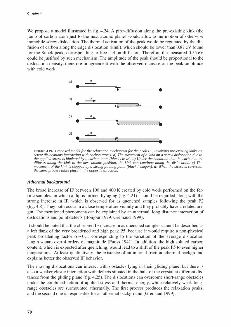
Chapter 4
70
We propose a model illustrated in fig. 4.24. A pipe-diffusion along the pre-existing kink (thejump of carbon atom just to the next atomic plane) would allow some motion of otherwiseimmobile screw dislocation. The thermal activation of the peak would be regulated by the dif-fusion of carbon along the edge dislocation (kink), which should be lower than 0.87 eV foundfor the Snoek peak, corresponding to free carbon diffusion. Therefore the measured 0.55 eVcould be justified by such mechanism. The amplitude of the peak should be proportional to thedislocation density, therefore in agreement with the observed increase of the peak amplitudewith cold work.
Athermal background
The broad increase of IF between 100 and 400 K created by cold work performed on the fer-ritic samples, in which a dip is formed by aging (fig. 4.21), should be regarded along with thestrong increase in IF, which is observed for as quenched samples following the peak P2(fig. 4.8). They both occur in a close temperature vicinity and they probably have a related ori-gin. The mentioned phenomena can be explained by an athermal, long distance interaction ofdislocations and point defects [Bonjour 1979, Gremaud 1999].
It should be noted that the observed IF increase in as quenched samples cannot be described asa left flank of the very broadened and high peak P5, because it would require a non-physicalpeak broadening factor α ≈ 0.1, corresponding to the variation of the average dislocationlength square over 4 orders of magnitude [Fuoss 1941]. In addition, the high soluted carboncontent, which is expected after quenching, would lead to a shift of the peak P5 to even highertemperatures. At least qualitatively, the existence of an internal friction athermal backgroundexplains better the observed IF behavior.
The moving dislocations can interact with obstacles lying in their gliding plane, but there isalso a weaker elastic interaction with defects situated in the bulk of the crystal at different dis-tances from the gliding plane (fig. 4.25). The dislocations can overcome short-range obstaclesunder the combined action of applied stress and thermal energy, while relatively weak long-range obstacles are surmounted athermally. The first process produces the relaxation peaks,and the second one is responsible for an athermal background [Gremaud 1999].
FIGURE 4.24. Proposed model for the relaxation mechanism for the peak P2, involving pre-existing kinks onscrew dislocations interacting with carbon atoms. a) The movement of a kink on a screw dislocation due tothe applied stress is hindered by a carbon atom (black circle). b) Under the condition that the carbon atomdiffuses along the kink to the next atomic position, the kink can continue along the dislocation. c) Themovement of the kink is stopped by a strong pinning point (black hexagon). d) When the stress is reversed,the same process takes place in the opposite direction.
σ
σ
σ
σ
a)
d)
c)
b)
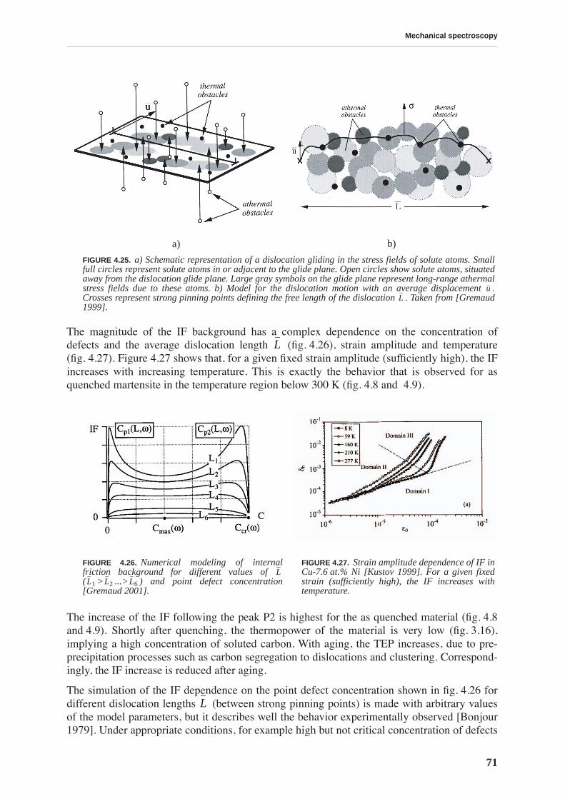
Mechanical spectroscopy
71
The magnitude of the IF background has a complex dependence on the concentration ofdefects and the average dislocation length (fig. 4.26), strain amplitude and temperature(fig. 4.27). Figure 4.27 shows that, for a given fixed strain amplitude (sufficiently high), the IFincreases with increasing temperature. This is exactly the behavior that is observed for asquenched martensite in the temperature region below 300 K (fig. 4.8 and 4.9).
The increase of the IF following the peak P2 is highest for the as quenched material (fig. 4.8and 4.9). Shortly after quenching, the thermopower of the material is very low (fig. 3.16),implying a high concentration of soluted carbon. With aging, the TEP increases, due to pre-precipitation processes such as carbon segregation to dislocations and clustering. Correspond-ingly, the IF increase is reduced after aging.
The simulation of the IF dependence on the point defect concentration shown in fig. 4.26 fordifferent dislocation lengths (between strong pinning points) is made with arbitrary valuesof the model parameters, but it describes well the behavior experimentally observed [Bonjour1979]. Under appropriate conditions, for example high but not critical concentration of defects
a) b)
FIGURE 4.25. a) Schematic representation of a dislocation gliding in the stress fields of solute atoms. Smallfull circles represent solute atoms in or adjacent to the glide plane. Open circles show solute atoms, situatedaway from the dislocation glide plane. Large gray symbols on the glide plane represent long-range athermalstress fields due to these atoms. b) Model for the dislocation motion with an average displacement .Crosses represent strong pinning points defining the free length of the dislocation . Taken from [Gremaud1999].
FIGURE 4.26. Numerical modeling of internalfriction background for different values of ( > ...> ) and point defect concentration[Gremaud 2001].
FIGURE 4.27. Strain amplitude dependence of IF inCu-7.6 at.% Ni [Kustov 1999]. For a given fixedstrain (sufficiently high), the IF increases withtemperature.
uL
L
LL1 L2 L6
L
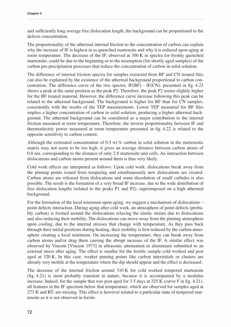
Chapter 4
72
and sufficiently long average free dislocation length, the background can be proportional to thedefects concentration.
The proportionality of the athermal internal friction to the concentration of carbon can explainwhy the increase of IF is highest in as quenched martensite and why it is reduced upon aging atroom temperature. The decrease of the IF, observed at 300 K in spectra for freshly quenchedmartensite, could be due to the beginning or to the resumption (for shortly aged samples) of thecarbon pre-precipitation processes that reduce the concentration of carbon in solid solution.
The difference of internal friction spectra for samples extracted from BF and CN treated filescan also be explained by the existence of the athermal background proportional to carbon con-centration. The difference curve of the two spectra, IF(BF) - IF(CN), presented in fig. 4.23shows a peak at the same position as the peak P2. Therefore, the peak P2 seems slightly higherfor the BF treated material. However, the difference curve increase following this peak can berelated to the athermal background. The background is higher for BF than for CN samples,consistently with the results of the TEP measurements. Lower TEP measured for BF filesimplies a higher concentration of carbon in solid solution, producing a higher athermal back-ground. The athermal background can be considered as a major contribution to the internalfriction measured at room temperature. Therefore, the inverse proportionality between IF andthermoelectric power measured at room temperature presented in fig. 4.22 is related to theopposite sensitivity to carbon content.
Although the estimated concentration of 0.5 wt.% carbon in solid solution in the martensiticmatrix may not seem to be too high, it gives an average distance between carbon atoms of0.8 nm, corresponding to the distance of only 2.8 martensite unit cells. An interaction betweendislocations and carbon atoms present around them is thus very likely.
Cold work effects are interpreted as follows. Upon cold work, dislocations break away fromthe pinning points issued from tempering and simultaneously new dislocations are created.Carbon atoms are released from dislocations and some dissolution of small carbides is alsopossible. The result is the formation of a very broad IF increase, due to the wide distribution offree dislocation lengths (related to the peaks P1 and P2), superimposed on a high athermalbackground.
For the formation of the local minimum upon aging, we suggest a mechanism of dislocations –point defects interaction. During aging after cold work, an atmosphere of point defects (proba-bly carbon) is formed around the dislocations relaxing the elastic strains due to dislocationsand also reducing their mobility. The dislocations can move away from the pinning atmosphereupon cooling, due to the internal stresses that change with temperature. As they pass backthrough their initial positions during heating, their mobility is first reduced by the carbon atmo-sphere creating a local minimum. On increasing the temperature, they can break away fromcarbon atoms and/or drag them causing the abrupt increase of the IF. A similar effect wasobserved by Vincent [Vincent 1973] in ultrasonic attenuation in aluminium submitted to anexternal stress after aging. The effect is smaller for the ferritic sample cold worked and postaged at 320 K. In this case, weaker pinning points like carbon interstitials or clusters arealready very mobile at the temperature where the dip should appear and the effect is decreased.
The decrease of the internal friction around 310 K for cold worked tempered martensite(fig. 4.21) is most probably transient in nature, because it is accompanied by a modulusincrease. Indeed, for the sample that was post aged for 3.5 days at 325 K (curve F in fig. 4.21),all features in the IF spectrum below that temperature, which are observed for samples aged at273 K and RT, are missing. This effect is however related to a particular state of tempered mar-tensite as it is not observed in ferrite.

Mechanical spectroscopy
73
High temperature background
At relatively high temperatures, the damping curve of most materials rises continuously to verylarge values of internal friction. This background is found to be higher in polycrystalline mate-rials than in single crystals, and it is higher for finer grain size. Therefore it is apparentlyrelated to grain boundary mechanisms [Nowick 1972a].
The internal friction spectra were not studied in detail for temperatures higher than 800 K. Thefirst reason is purely practical: 800 K is the upper temperature limit of the installations used.But a more important reason is that the martensitic structure, which is the main object of thiswork, undergoes major changes already at 500 K. Therefore the study of the high temperaturebehavior is out of the scope of this work. Some purely qualitative observations should be how-ever mentioned.
The IF background that is observed following the peak P5 is much higher for low than for highfrequency measurements (fig. 4.10), therefore implying a thermally activated relaxation mech-anism. The background decreases after 1 h tempering at 800 K indicating that the structure isnot stable. Finally, the background following the peak P5 for the ferritic structure is found to besignificantly lower than the one for tempered martensite and bainite (fig. 4.17). The micro-structure of ferrite is much coarser (confirmed by TEM imaging), which supports the hypothe-sis that the background is grain boundary related.
4.3 Conclusions
The martensitic structure is characterized and distinguished by a rich internal friction spectrumcomposed of several overlapping relaxation and transition phenomena. The relaxation mecha-nisms are related to the interaction of dislocations and point defects and their mobility.
The peak P1 is interpreted as Snoek-Köster hydrogen peak. A mechanism is proposed for thepeak P2, involving pipe-diffusion along kinks on screw dislocations. The tempering processes(for aged material) start upon heating over 375 K, causing a decrease of the internal frictionand an increase of the Young’s modulus. Thus peaks P3 and most likely P4 are not relaxationpeaks, but products of these tempering effects. The peak P5 is interpreted as a Snoek-Köstercarbon peak. The increase of the IF observed for as quenched samples is attributed to an ather-mal background proportional to the amount of carbon in solid solution. This mechanism is alsoresponsible for the difference in IF between CN and BF treated material.
The spectra obtained by mechanical spectroscopy show that the material continuously changesdue to the tempering. Therefore, tempering effects will be studied in more details in the follow-ing chapter.

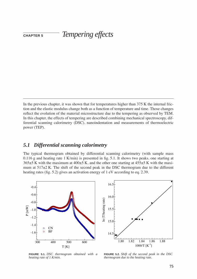
75
CHAPTER 5
Tempering effects
In the previous chapter, it was shown that for temperatures higher than 375 K the internal fric-tion and the elastic modulus change both as a function of temperature and time. Those changesreflect the evolution of the material microstructure due to the tempering as observed by TEM.In this chapter, the effects of tempering are described combining mechanical spectroscopy, dif-ferential scanning calorimetry (DSC), nanoindentation and measurements of thermoelectricpower (TEP).
5.1 Differential scanning calorimetry
The typical thermogram obtained by differential scanning calorimetry (with sample mass0.116 g and heating rate 1 K/min) is presented in fig. 5.1. It shows two peaks, one starting at365±5 K with the maximum at 400±5 K, and the other one starting at 455±5 K with the maxi-mum at 517±2 K. The shift of the second peak in the DSC thermogram due to the differentheating rates (fig. 5.2) gives an activation energy of 1 eV according to eq. 2.39.
FIGURE 5.1.
DSC thermogram obtained with aheating rate of 1 K/min.
FIGURE 5.2.
Shift of the second peak in the DSCthermogram due to the heating rate.
-1.6
-1.4
-1.2
-1.0
-0.8
-0.6
-0.4
P [m
W]
600500400300T [K]
CN BF
16.5
16.0
15.5
15.0
14.5
ln (
T/h
eatin
g ra
te)
1.881.861.841.821.801000/T [K-1]
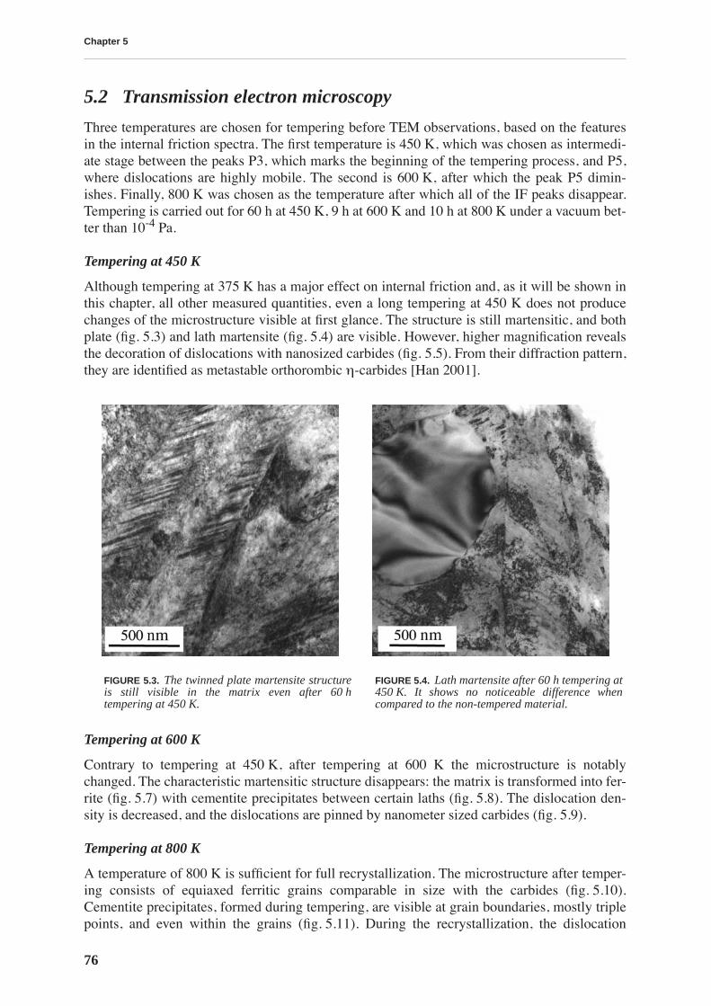
Chapter 5
76
5.2 Transmission electron microscopy
Three temperatures are chosen for tempering before TEM observations, based on the featuresin the internal friction spectra. The first temperature is 450 K, which was chosen as intermedi-ate stage between the peaks P3, which marks the beginning of the tempering process, and P5,where dislocations are highly mobile. The second is 600 K, after which the peak P5 dimin-ishes. Finally, 800 K was chosen as the temperature after which all of the IF peaks disappear.Tempering is carried out for 60 h at 450 K, 9 h at 600 K and 10 h at 800 K under a vacuum bet-ter than 10
-4
Pa.
Tempering at 450 K
Although tempering at 375 K has a major effect on internal friction and, as it will be shown inthis chapter, all other measured quantities, even a long tempering at 450 K does not producechanges of the microstructure visible at first glance. The structure is still martensitic, and bothplate (fig. 5.3) and lath martensite (fig. 5.4) are visible. However, higher magnification revealsthe decoration of dislocations with nanosized carbides (fig. 5.5). From their diffraction pattern,they are identified as metastable orthorombic
η
-carbides [Han 2001].
Tempering at 600 K
Contrary to tempering at 450 K, after tempering at 600 K the microstructure is notablychanged. The characteristic martensitic structure disappears: the matrix is transformed into fer-rite (fig. 5.7) with cementite precipitates between certain laths (fig. 5.8). The dislocation den-sity is decreased, and the dislocations are pinned by nanometer sized carbides (fig. 5.9).
Tempering at 800 K
A temperature of 800 K is sufficient for full recrystallization. The microstructure after temper-ing consists of equiaxed ferritic grains comparable in size with the carbides (fig. 5.10).Cementite precipitates, formed during tempering, are visible at grain boundaries, mostly triplepoints, and even within the grains (fig. 5.11). During the recrystallization, the dislocation
FIGURE 5.3.
The twinned plate martensite structureis still visible in the matrix even after 60 htempering at 450 K.
FIGURE 5.4.
Lath martensite after 60 h tempering at450 K. It shows no noticeable difference whencompared to the non-tempered material.
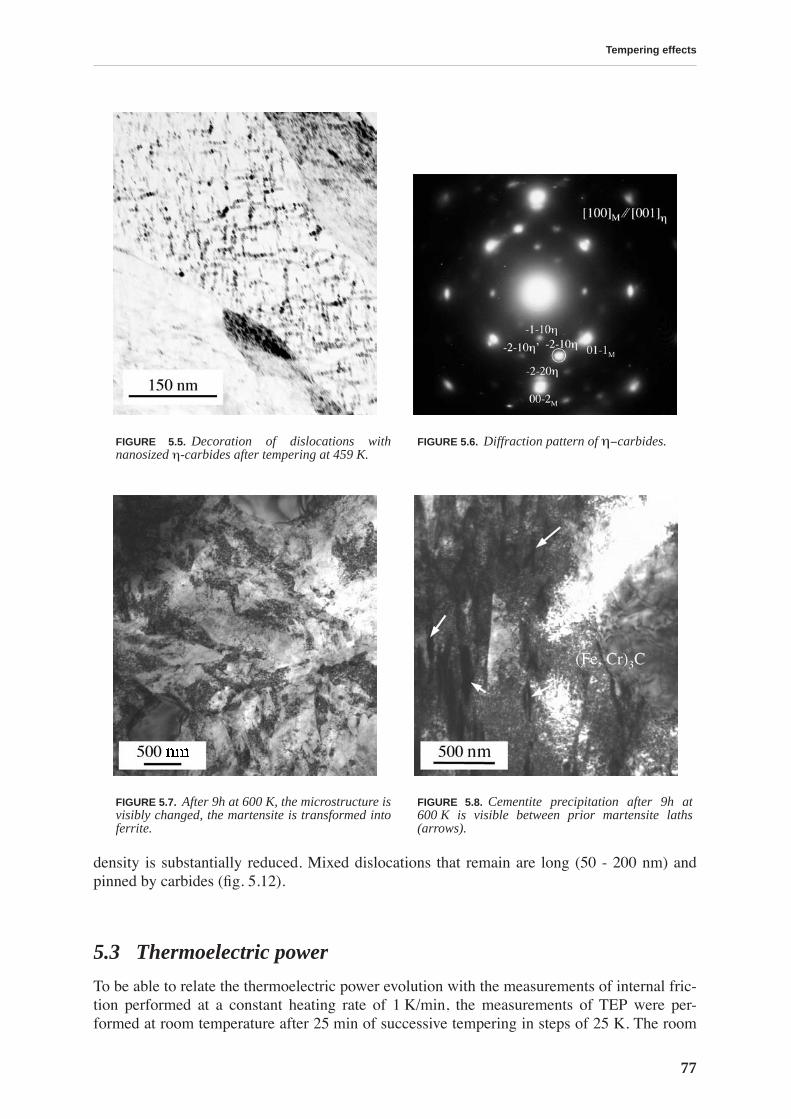
Tempering effects
77
density is substantially reduced. Mixed dislocations that remain are long (50 - 200 nm) andpinned by carbides (fig. 5.12).
5.3 Thermoelectric power
To be able to relate the thermoelectric power evolution with the measurements of internal fric-tion performed at a constant heating rate of 1 K/min, the measurements of TEP were per-formed at room temperature after 25 min of successive tempering in steps of 25 K. The room
FIGURE 5.5.
Decoration of dislocations withnanosized
η
-carbides after tempering at 459 K.
FIGURE 5.6.
Diffraction pattern of
η
−
carbides.
FIGURE 5.7.
After 9h at 600 K, the microstructure isvisibly changed, the martensite is transformed intoferrite.
FIGURE 5.8.
Cementite precipitation after 9h at600 K is visible between prior martensite laths(arrows).
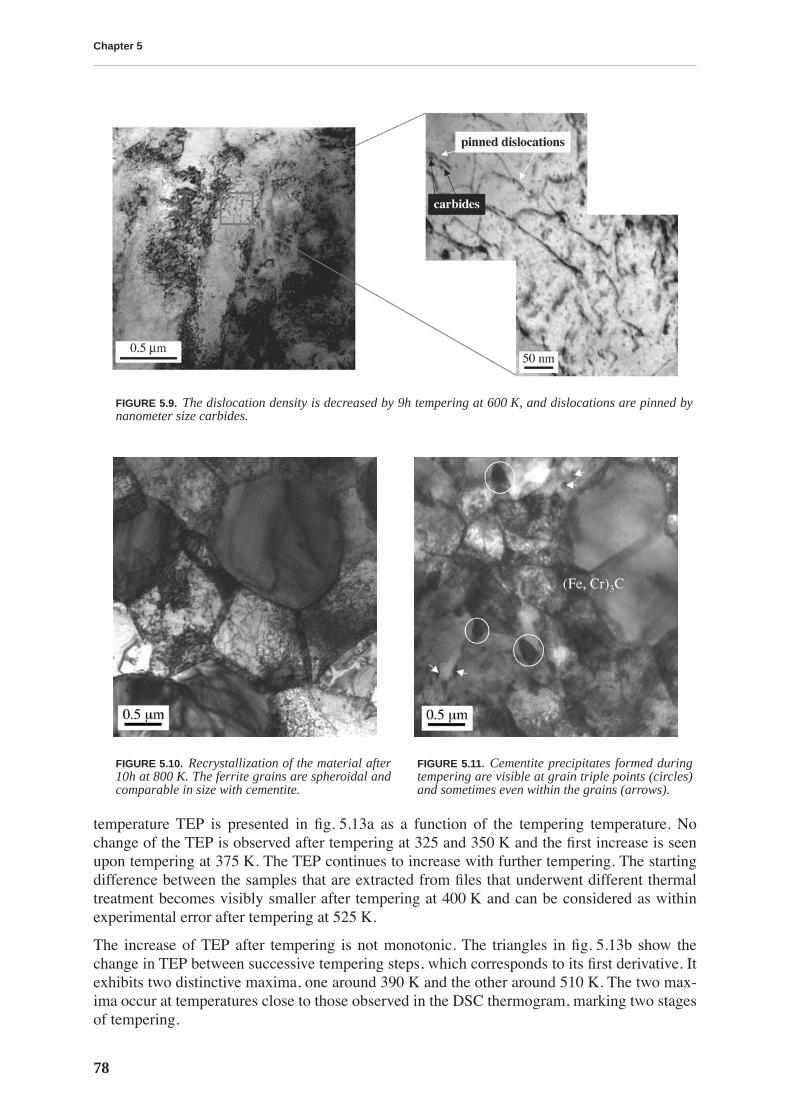
Chapter 5
78
temperature TEP is presented in fig. 5.13a as a function of the tempering temperature. Nochange of the TEP is observed after tempering at 325 and 350 K and the first increase is seenupon tempering at 375 K. The TEP continues to increase with further tempering. The startingdifference between the samples that are extracted from files that underwent different thermaltreatment becomes visibly smaller after tempering at 400 K and can be considered as withinexperimental error after tempering at 525 K.
The increase of TEP after tempering is not monotonic. The triangles in fig. 5.13b show thechange in TEP between successive tempering steps, which corresponds to its first derivative. Itexhibits two distinctive maxima, one around 390 K and the other around 510 K. The two max-ima occur at temperatures close to those observed in the DSC thermogram, marking two stagesof tempering.
FIGURE 5.9.
The dislocation density is decreased by 9h tempering at 600 K, and dislocations are pinned bynanometer size carbides.
FIGURE 5.10.
Recrystallization of the material after10h at 800 K. The ferrite grains are spheroidal andcomparable in size with cementite.
FIGURE 5.11.
Cementite precipitates formed duringtempering are visible at grain triple points (circles)and sometimes even within the grains (arrows).
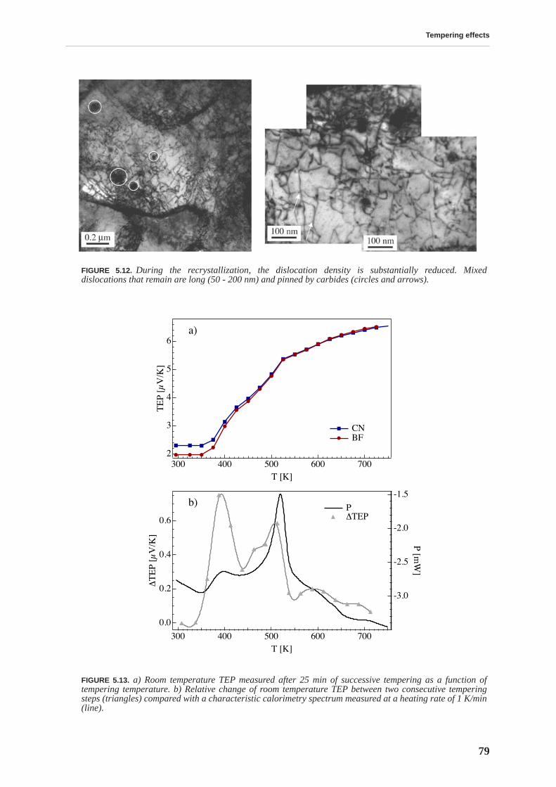
Tempering effects
79
FIGURE 5.12.
During the recrystallization, the dislocation density is substantially reduced. Mixeddislocations that remain are long (50 - 200 nm) and pinned by carbides (circles and arrows).
FIGURE 5.13.
a) Room temperature TEP measured after 25 min of successive tempering as a function oftempering temperature. b) Relative change of room temperature TEP between two consecutive temperingsteps (triangles) compared with a characteristic calorimetry spectrum measured at a heating rate of 1 K/min(line).
6
5
4
3
2
TE
P [µ
V/K
]
700600500400300T [K]
a)
CN BF
-3.0
-2.5
-2.0
-1.5
P [mW
]
700600500400300T [K]
0.6
0.4
0.2
0.0
∆T
EP
[µV
/K]
b) P ∆TEP
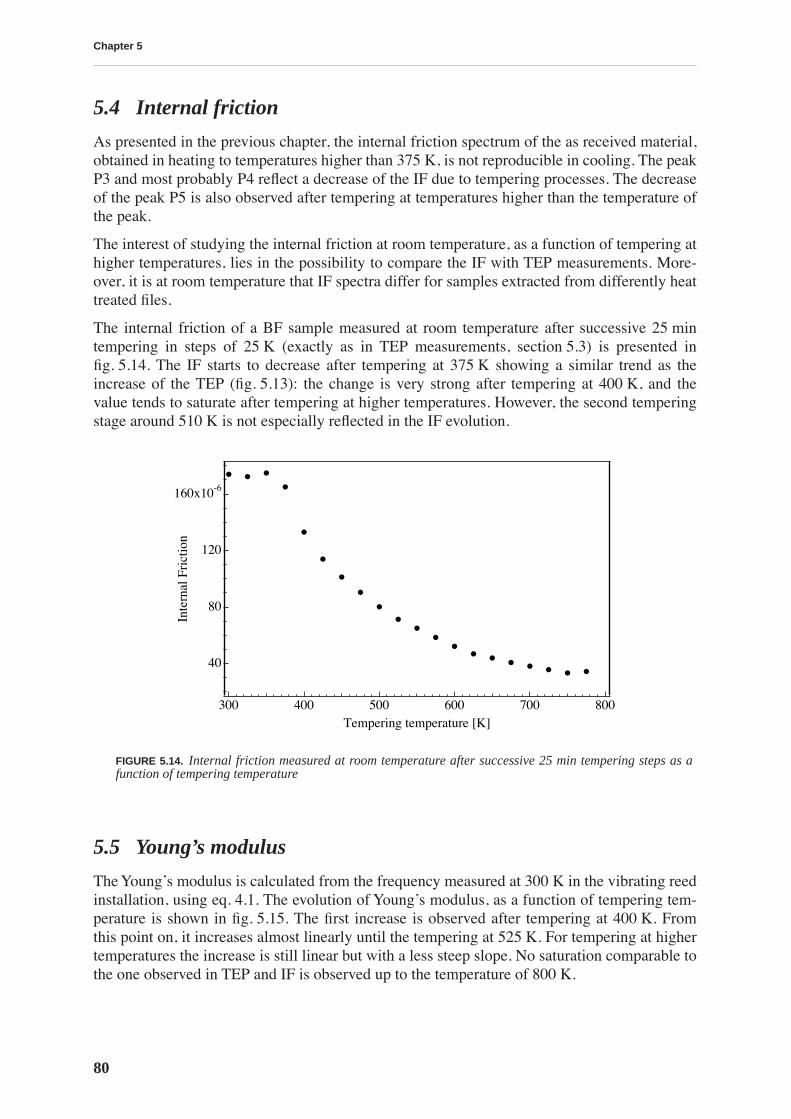
Chapter 5
80
5.4 Internal friction
As presented in the previous chapter, the internal friction spectrum of the as received material,obtained in heating to temperatures higher than 375 K, is not reproducible in cooling. The peakP3 and most probably P4 reflect a decrease of the IF due to tempering processes. The decreaseof the peak P5 is also observed after tempering at temperatures higher than the temperature ofthe peak.
The interest of studying the internal friction at room temperature, as a function of tempering athigher temperatures, lies in the possibility to compare the IF with TEP measurements. More-over, it is at room temperature that IF spectra differ for samples extracted from differently heattreated files.
The internal friction of a BF sample measured at room temperature after successive 25 mintempering in steps of 25 K (exactly as in TEP measurements, section 5.3) is presented infig. 5.14. The IF starts to decrease after tempering at 375 K showing a similar trend as theincrease of the TEP (fig. 5.13): the change is very strong after tempering at 400 K, and thevalue tends to saturate after tempering at higher temperatures. However, the second temperingstage around 510 K is not especially reflected in the IF evolution.
5.5 Young’s modulus
The Young’s modulus is calculated from the frequency measured at 300 K in the vibrating reedinstallation, using eq. 4.1. The evolution of Young’s modulus, as a function of tempering tem-perature is shown in fig. 5.15. The first increase is observed after tempering at 400 K. Fromthis point on, it increases almost linearly until the tempering at 525 K. For tempering at highertemperatures the increase is still linear but with a less steep slope. No saturation comparable tothe one observed in TEP and IF is observed up to the temperature of 800 K.
FIGURE 5.14.
Internal friction measured at room temperature after successive 25 min tempering steps as afunction of tempering temperature
160x10-6
120
80
40
Inte
rnal
Fri
ctio
n
800700600500400300Tempering temperature [K]
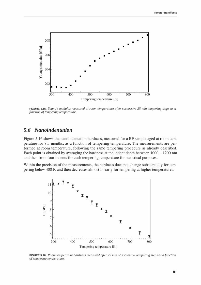
Tempering effects
81
5.6 Nanoindentation
Figure 5.16 shows the nanoindentation hardness, measured for a BF sample aged at room tem-perature for 8.5 months, as a function of tempering temperature. The measurements are per-formed at room temperature, following the same tempering procedure as already described.Each point is obtained by averaging the hardness at the indent depth between 1000 – 1200 nmand then from four indents for each tempering temperature for statistical purposes.
Within the precision of the measurements, the hardness does not change substantially for tem-pering below 400 K and then decreases almost linearly for tempering at higher temperatures.
FIGURE 5.15.
Young’s modulus measured at room temperature after successive 25 min tempering steps as afunction of tempering temperature.
FIGURE 5.16.
Room temperature hardness measured after 25 min of successive tempering steps as a functionof tempering temperature.
208
206
204
202
You
ng's
mod
ulus
[G
Pa]
800700600500400300Tempering temperature [K]
11
10
9
8
7
6
5
H [
GPa
]
800700600500400300
Tempering temperature [K]
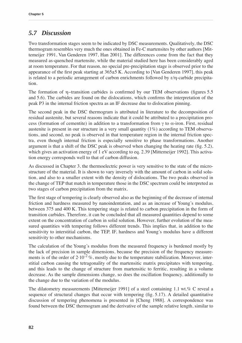
Chapter 5
82
5.7 Discussion
Two transformation stages seem to be indicated by DSC measurements. Qualitatively, the DSCthermogram resembles very much the ones obtained in Fe-C martensites by other authors [Mit-temeijer 1991, Van Genderen 1997, Han 2001]. The differences come from the fact that theymeasured as-quenched martensite, while the material studied here has been considerably agedat room temperature. For that reason, no special pre-precipitation stage is observed prior to theappearance of the first peak starting at 365±5 K. According to [Van Genderen 1997], this peakis related to a periodic arrangement of carbon enrichments followed by
ε
/
η
-carbide precipita-tion.
The formation of
η−
transition carbides is confirmed by our TEM observations (figures 5.5and 5.6). The carbides are found on the dislocations, which confirms the interpretation of thepeak P3 in the internal friction spectra as an IF decrease due to dislocation pinning.
The second peak in the DSC thermogram is attributed in literature to the decomposition ofresidual austenite, but several reasons indicate that it could be attributed to a precipitation pro-cess (formation of cementite) in addition to a transformation from
γ
to
α
-iron. First, residualaustenite is present in our structure in a very small quantity (1%) according to TEM observa-tions, and second, no peak is observed in that temperature region in the internal friction spec-tra, even though internal friction is especially sensitive to phase transformations. Anotherargument is that a shift of the DSC peak is observed when changing the heating rate (fig. 5.2),which gives an activation energy of 1 eV according to eq. 2.39 [Mittemeijer 1992]. This activa-tion energy corresponds well to that of carbon diffusion.
As discussed in Chapter 3, the thermoelectric power is very sensitive to the state of the micro-structure of the material. It is shown to vary inversely with the amount of carbon in solid solu-tion, and also to a smaller extent with the density of dislocations. The two peaks observed inthe change of TEP that match in temperature those in the DSC spectrum could be interpreted astwo stages of carbon precipitation from the matrix.
The first stage of tempering is clearly observed also as the beginning of the decrease of internalfriction and hardness measured by nanoindentation, and as an increase of Young’s modulus,between 375 and 400 K. This tempering stage is related to carbon precipitation in the form oftransition carbides. Therefore, it can be concluded that all measured quantities depend to someextent on the concentration of carbon in solid solution. However, further evolution of the mea-sured quantities with tempering follows different trends. This implies that, in addition to thesensitivity to interstitial carbon, the TEP, IF, hardness and Young’s modulus have a differentsensitivity to other mechanisms.
The calculation of the Young’s modulus from the measured frequency is burdened mostly bythe lack of precision in sample dimensions, because the precision of the frequency measure-ments is of the order of 2·10
-2
%, mostly due to the temperature stabilization. Moreover, inter-stitial carbon causing the tetragonality of the martensitic matrix precipitates with tempering,and this leads to the change of structure from martensitic to ferritic, resulting in a volumedecrease. As the sample dimensions change, so does the oscillation frequency, additionally tothe change due to the variation of the modulus.
The dilatometry measurements [Mittemeijer 1991] of a steel containing 1.1 wt.% C reveal asequence of structural changes that occur with tempering (fig. 5.17). A detailed quantitativediscussion of tempering phenomena is presented in [Cheng 1988]. A correspondence wasfound between the DSC thermogram and the derivative of the sample relative length, similar to
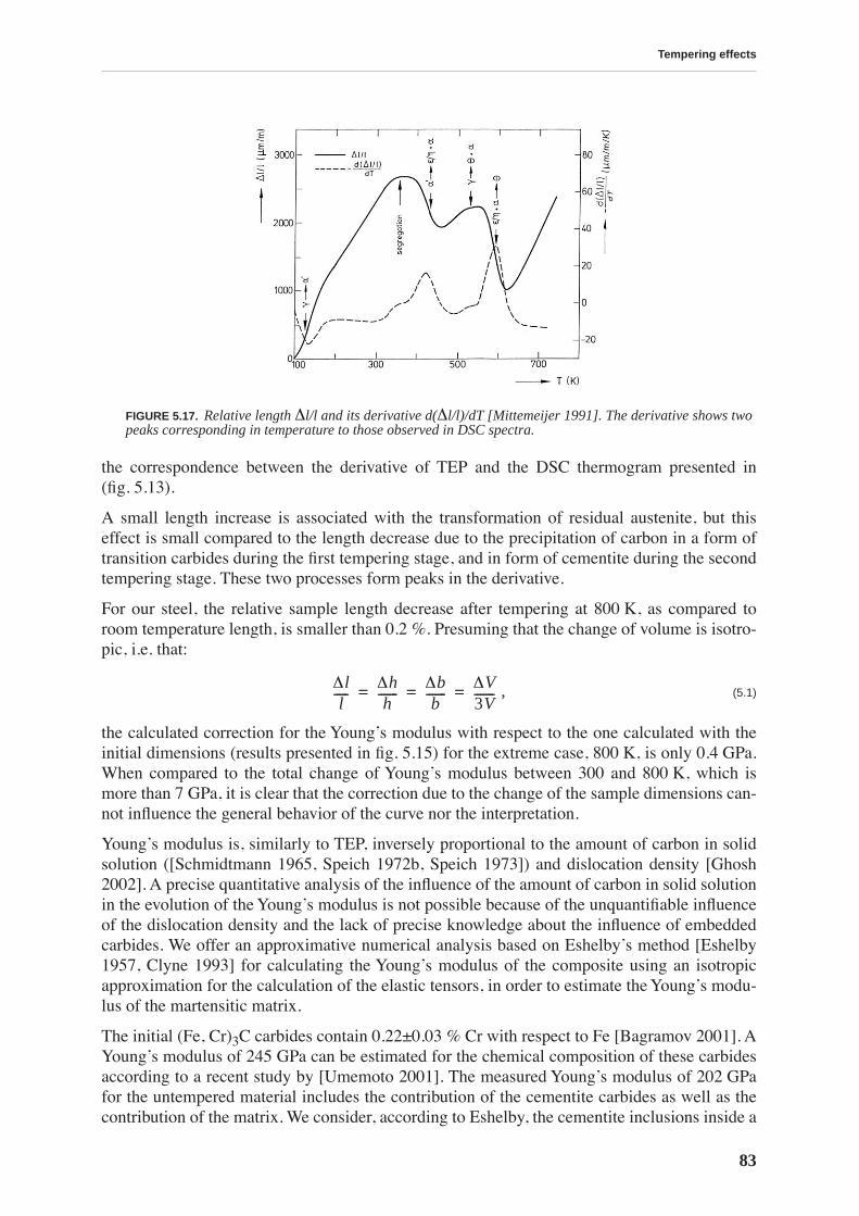
Tempering effects
83
the correspondence between the derivative of TEP and the DSC thermogram presented in(fig. 5.13).
A small length increase is associated with the transformation of residual austenite, but thiseffect is small compared to the length decrease due to the precipitation of carbon in a form oftransition carbides during the first tempering stage, and in form of cementite during the secondtempering stage. These two processes form peaks in the derivative.
For our steel, the relative sample length decrease after tempering at 800 K, as compared toroom temperature length, is smaller than 0.2 %. Presuming that the change of volume is isotro-pic, i.e. that:
,
(5.1)
the calculated correction for the Young’s modulus with respect to the one calculated with theinitial dimensions (results presented in fig. 5.15) for the extreme case, 800 K, is only 0.4 GPa.When compared to the total change of Young’s modulus between 300 and 800 K, which ismore than 7 GPa, it is clear that the correction due to the change of the sample dimensions can-not influence the general behavior of the curve nor the interpretation.
Young’s modulus is, similarly to TEP, inversely proportional to the amount of carbon in solidsolution ([Schmidtmann 1965, Speich 1972b, Speich 1973]) and dislocation density [Ghosh2002]. A precise quantitative analysis of the influence of the amount of carbon in solid solutionin the evolution of the Young’s modulus is not possible because of the unquantifiable influenceof the dislocation density and the lack of precise knowledge about the influence of embeddedcarbides. We offer an approximative numerical analysis based on Eshelby’s method [Eshelby1957, Clyne 1993] for calculating the Young’s modulus of the composite using an isotropicapproximation for the calculation of the elastic tensors, in order to estimate the Young’s modu-lus of the martensitic matrix.
The initial (Fe, Cr)
3
C carbides contain 0.22±0.03 % Cr with respect to Fe [Bagramov 2001]. AYoung’s modulus of 245 GPa can be estimated for the chemical composition of these carbidesaccording to a recent study by [Umemoto 2001]. The measured Young’s modulus of 202 GPafor the untempered material includes the contribution of the cementite carbides as well as thecontribution of the matrix. We consider, according to Eshelby, the cementite inclusions inside a
FIGURE 5.17.
Relative length
∆
l/l and its derivative d(
∆
l/l)/dT [Mittemeijer 1991]. The derivative shows twopeaks corresponding in temperature to those observed in DSC spectra.
∆ll
-----∆hh
-------∆bb
-------∆V3V-------= = =
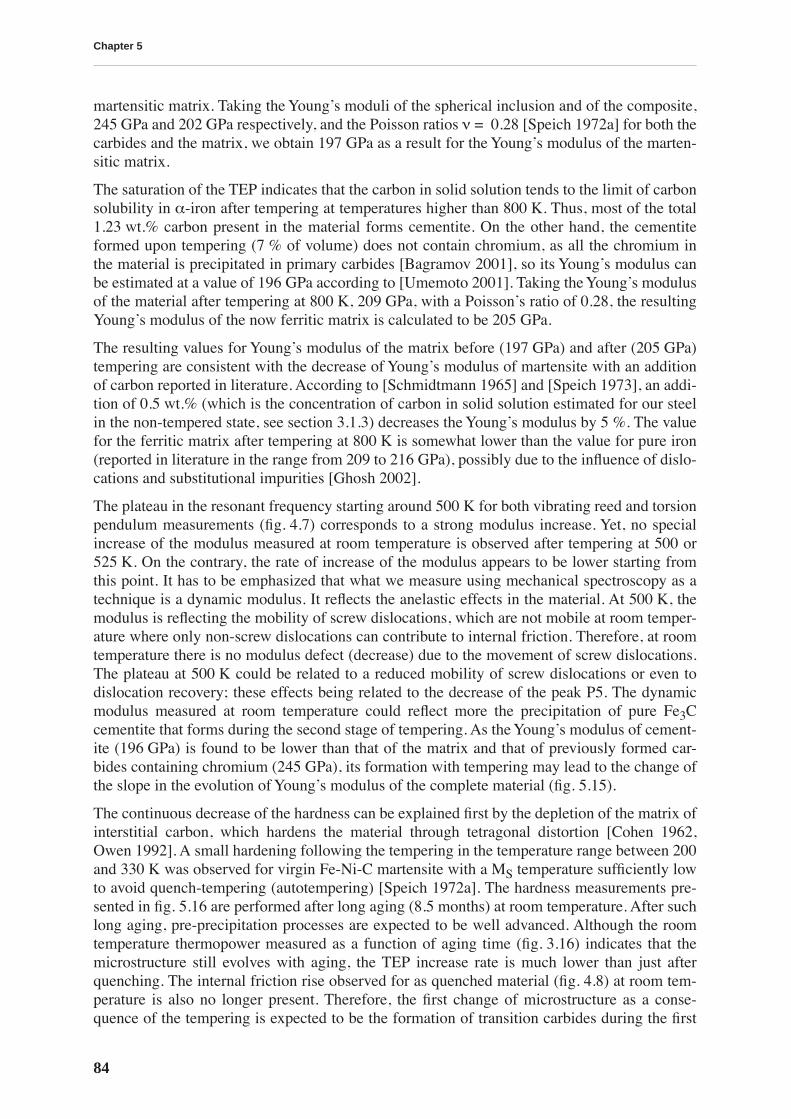
Chapter 5
84
martensitic matrix. Taking the Young’s moduli of the spherical inclusion and of the composite,245 GPa and 202 GPa respectively, and the Poisson ratios
ν
= 0.28 [Speich 1972a] for both thecarbides and the matrix, we obtain 197 GPa as a result for the Young’s modulus of the marten-sitic matrix.
The saturation of the TEP indicates that the carbon in solid solution tends to the limit of carbonsolubility in
α
-iron after tempering at temperatures higher than 800 K. Thus, most of the total1.23 wt.% carbon present in the material forms cementite. On the other hand, the cementiteformed upon tempering (7 % of volume) does not contain chromium, as all the chromium inthe material is precipitated in primary carbides [Bagramov 2001], so its Young’s modulus canbe estimated at a value of 196 GPa according to [Umemoto 2001]. Taking the Young’s modulusof the material after tempering at 800 K, 209 GPa, with a Poisson’s ratio of 0.28, the resultingYoung’s modulus of the now ferritic matrix is calculated to be 205 GPa.
The resulting values for Young’s modulus of the matrix before (197 GPa) and after (205 GPa)tempering are consistent with the decrease of Young’s modulus of martensite with an additionof carbon reported in literature. According to [Schmidtmann 1965] and [Speich 1973], an addi-tion of 0.5 wt.% (which is the concentration of carbon in solid solution estimated for our steelin the non-tempered state, see section 3.1.3) decreases the Young’s modulus by 5 %. The valuefor the ferritic matrix after tempering at 800 K is somewhat lower than the value for pure iron(reported in literature in the range from 209 to 216 GPa), possibly due to the influence of dislo-cations and substitutional impurities [Ghosh 2002].
The plateau in the resonant frequency starting around 500 K for both vibrating reed and torsionpendulum measurements (fig. 4.7) corresponds to a strong modulus increase. Yet, no specialincrease of the modulus measured at room temperature is observed after tempering at 500 or525 K. On the contrary, the rate of increase of the modulus appears to be lower starting fromthis point. It has to be emphasized that what we measure using mechanical spectroscopy as atechnique is a dynamic modulus. It reflects the anelastic effects in the material. At 500 K, themodulus is reflecting the mobility of screw dislocations, which are not mobile at room temper-ature where only non-screw dislocations can contribute to internal friction. Therefore, at roomtemperature there is no modulus defect (decrease) due to the movement of screw dislocations.The plateau at 500 K could be related to a reduced mobility of screw dislocations or even todislocation recovery; these effects being related to the decrease of the peak P5. The dynamicmodulus measured at room temperature could reflect more the precipitation of pure Fe
3
Ccementite that forms during the second stage of tempering. As the Young’s modulus of cement-ite (196 GPa) is found to be lower than that of the matrix and that of previously formed car-bides containing chromium (245 GPa), its formation with tempering may lead to the change ofthe slope in the evolution of Young’s modulus of the complete material (fig. 5.15).
The continuous decrease of the hardness can be explained first by the depletion of the matrix ofinterstitial carbon, which hardens the material through tetragonal distortion [Cohen 1962,Owen 1992]. A small hardening following the tempering in the temperature range between 200and 330 K was observed for virgin Fe-Ni-C martensite with a M
S
temperature sufficiently lowto avoid quench-tempering (autotempering) [Speich 1972a]. The hardness measurements pre-sented in fig. 5.16 are performed after long aging (8.5 months) at room temperature. After suchlong aging, pre-precipitation processes are expected to be well advanced. Although the roomtemperature thermopower measured as a function of aging time (fig. 3.16) indicates that themicrostructure still evolves with aging, the TEP increase rate is much lower than just afterquenching. The internal friction rise observed for as quenched material (fig. 4.8) at room tem-perature is also no longer present. Therefore, the first change of microstructure as a conse-quence of the tempering is expected to be the formation of transition carbides during the first

Tempering effects
85
tempering stage, starting at 375 K. Within the experimental precision no hardening due to thisprecipitation is observed, therefore excluding the hardening by dislocation pinning by car-bides, and supporting the hypothesis of solid-solution hardening.
The decrease of the hardness at higher temperatures should be attributed to the formation ofcoarse cementite and to recrystallization [Speich 1972a], the processes that are observed byTEM (figures 5.7 to 5.12) for samples tempered at 600 and 800 K.
The decrease of the dislocation density and the increase of the dislocation length observed byTEM after tempering at 600 and especially after 800 K confirm the explanation given for thedecrease of the peak P5 amplitude, given in the previous chapter. However, the similaritybetween evolution trends (or in better words reciprocity) of TEP and IF measured at room tem-perature points to a strong dependence of the room temperature IF on the carbon concentration.
5.8 Conclusions
The first stage of tempering in our material starts around 375 K as manifested by a peak in thecalorimetry thermogram. It is related to the precipitation of carbon in the martensite in form oftransition
η
-carbides. This tempering stage is reflected by a first increase of the TEP andYoung’s modulus and by a decrease of the internal friction and hardness. It implies that allthese quantities are sensitive to the concentration of carbon in solid solution in the martensiticmatrix. It is thus of great interest to determine the carbon concentration and its evolution withtempering quantitatively. For this purpose, experiments with X-ray diffraction are performed.The results and further interpretation of both material evolution during tempering and of thedifferences in mechanical properties resulting from the two types of thermal treatment of thefiles are presented in the following chapter.

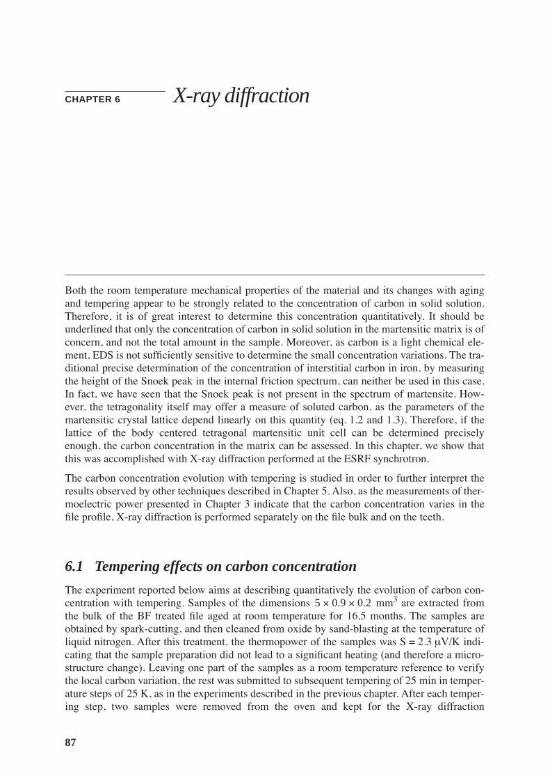
87
CHAPTER 6
X-ray diffraction
Both the room temperature mechanical properties of the material and its changes with agingand tempering appear to be strongly related to the concentration of carbon in solid solution.Therefore, it is of great interest to determine this concentration quantitatively. It should beunderlined that only the concentration of carbon in solid solution in the martensitic matrix is ofconcern, and not the total amount in the sample. Moreover, as carbon is a light chemical ele-ment, EDS is not sufficiently sensitive to determine the small concentration variations. The tra-ditional precise determination of the concentration of interstitial carbon in iron, by measuringthe height of the Snoek peak in the internal friction spectrum, can neither be used in this case.In fact, we have seen that the Snoek peak is not present in the spectrum of martensite. How-ever, the tetragonality itself may offer a measure of soluted carbon, as the parameters of themartensitic crystal lattice depend linearly on this quantity (eq. 1.2 and 1.3). Therefore, if thelattice of the body centered tetragonal martensitic unit cell can be determined preciselyenough, the carbon concentration in the matrix can be assessed. In this chapter, we show thatthis was accomplished with X-ray diffraction performed at the ESRF synchrotron.
The carbon concentration evolution with tempering is studied in order to further interpret theresults observed by other techniques described in Chapter 5. Also, as the measurements of ther-moelectric power presented in Chapter 3 indicate that the carbon concentration varies in thefile profile, X-ray diffraction is performed separately on the file bulk and on the teeth.
6.1 Tempering effects on carbon concentration
The experiment reported below aims at describing quantitatively the evolution of carbon con-centration with tempering. Samples of the dimensions mm
3
are extracted fromthe bulk of the BF treated file aged at room temperature for 16.5 months. The samples areobtained by spark-cutting, and then cleaned from oxide by sand-blasting at the temperature ofliquid nitrogen. After this treatment, the thermopower of the samples was S = 2.3
µ
V/K indi-cating that the sample preparation did not lead to a significant heating (and therefore a micro-structure change). Leaving one part of the samples as a room temperature reference to verifythe local carbon variation, the rest was submitted to subsequent tempering of 25 min in temper-ature steps of 25 K, as in the experiments described in the previous chapter. After each temper-ing step, two samples were removed from the oven and kept for the X-ray diffraction
5 0.9 0.2××
Chapter 6
88
experiment. The X-ray diffraction spectra are obtained in transmission, using the wavelength
λ
= 0.35037 Å.
The diffraction spectra in the 2
θ
range (see section 2.2.3 and eq. 2.1 and 2.2) of the peak{110}/{011} of the martensite
are presented in fig. 6.1. No significant difference among refer-ence (non-tempered) samples spectra is observed, so only one spectrum is displayed.
In fig. 6.1a, the spectra are plotted with the measured intensity normalized to the incident beamintensity. The peak {110}/{011} of the martensite strongly sharpens with tempering, so thatthe reduction in peak width is followed by an increase of the peak height. Furthermore, asharpening and later on an increase of the cementite peaks is observed (for example at2
θ
= 9.99 º). The amplitude of the {110}/{011} peak is also influenced by the sample dimen-sions (the amount of matter producing the diffraction spectrum). The small variation of thesample width (ranging from 0.85 to 1 mm) is the cause of the small irregularity in steps of thepeak sharpening.
In fig. 6.1b, the spectra are plotted with the intensity normalized to the height of the {110}/{011} martensite peak. In this scale, it is visible that the peak remains unchanged by temperingup to 350 K, and the first small change is observed after tempering at 375 K, followed by astrong sharpening of the peak after tempering at 400 K. As it is the peak {011} that best com-bines a high sensitivity to tetragonalization (see paragraph 2.2.3) together with a high intensity(for an ideal tetragonal structure the intensity of the peak {011} is twice the intensity of thepeak {110}), the change between tempering steps is more evident on the left flank of the com-posed {110}/{011} peak.
The strongest residual austenite peak, {111}
a
, that should be positioned in the spectrum at2
θ=
9.66º, is hidden below the strongest martensite peak, {110}/{011}. Nevertheless, threeresidual austenite peaks are clearly visible in the spectrum between 10.8 and 20.6º of 2
θ
(fig. 6.2) up to the tempering at 500 K, when the peaks amplitudes decrease. After tempering at525 K, the peaks are completely erased indicating the complete transformation of residual aus-tenite to ferrite and cementite. The volume fraction of residual austenite cannot be determinedfrom the spectrum with sufficient precision. The relative intensities of the peaks are not inagreement with theoretical and measured values possibly due to the preferred orientation. Therough estimation of the amount of residual austenite however gives a value between 4 and10 vol.%. This is more than estimated from the TEM images (1 %).
No transition carbide peaks [Van Genderen 1993] are found in the spectrum, regardless of thetempering temperature. The probable reason is their nanometer size.
6.1.1 Carbon content fitting
The concentration of carbon in solid solution in the martensitic matrix is calculated by fittingthe martensite double peaks ({110}/{011}, {200}/{002}, {211}/{112} and {220}/{022})using an iterative procedure. The peak positions are fitted using the Igor Pro (Wavemetrics)software. A gaussian peak shape is found to give the best fit. The peak positions are then com-pared with those calculated for the bct lattice (space group I4/mmm) using Checkcell. The cal-culation of the peak positions was based on eq. 1.2 and 1.3 that describe the change of thelattice parameters depending on the carbon concentration. The expected peak positions arethen reintroduced as a new guess for the Igor fitting procedure. The procedure is repeated untila satisfactory correspondence of all peak positions with the tetragonal structure is found inCheckcell. The cementite peaks are fitted but not refined with the structure. The residual auste-nite (when present) is fitted using {200}
a
peak at . Then, the related intensity of{111}
a
at is fixed for the fit of the martensite {110}/{011} peak that overlays it. 2θ 11.16°=
2θ 9.66°=

X-ray diffraction
89
FIGURE 6.1.
Effect of tempering on peak {110}/{011} of martensite. a) Spectra normalized to the intensity ofincident beam. b) Spectra normalized to the height of the {110}/{011} peak.
Cou
nts
a.u.
10.410.210.09.89.69.42Θ [˚]
10.410.210.09.89.69.42θ [˚]
3
25
20
15
10
5
Cou
nts
(nor
mal
ized
)
RT 325 K 350 K 375 K 400 K 425 K 450 K 475 K 500 K 525 K 550 K 575 K 600 K 625 K 650 K 675 K 700 K 725 K 750 K 775 K 800 K 24h @ 800 K
{110}/{011}ma)
b)
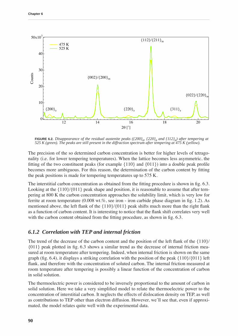
Chapter 6
90
The precision of the so determined carbon concentration is better for higher levels of tetrago-nality (i.e. for lower tempering temperatures). When the lattice becomes less asymmetric, thefitting of the two constituent peaks (for example {110} and {011}) into a double peak profilebecomes more ambiguous. For this reason, the determination of the carbon content by fittingthe peak positions is made for tempering temperatures up to 575 K.
The interstitial carbon concentration as obtained from the fitting procedure is shown in fig. 6.3.Looking at the {110}/{011} peak shape and position, it is reasonable to assume that after tem-pering at 800 K the carbon concentration approaches the solubility limit, which is very low forferrite at room temperature (0.008 wt.%, see iron - iron carbide phase diagram in fig. 1.2). Asmentioned above, the left flank of the {110}/{011} peak shifts much more than the right flankas a function of carbon content. It is interesting to notice that the flank shift correlates very wellwith the carbon content obtained from the fitting procedure, as shown in fig. 6.3.
6.1.2 Correlation with TEP and internal friction
The trend of the decrease of the carbon content and the position of the left flank of the {110}/{011} peak plotted in fig. 6.3 shows a similar trend as the decrease of internal friction mea-sured at room temperature after tempering. Indeed, when internal friction is shown on the samegraph (fig. 6.4), it displays a striking correlation with the position of the peak {110}/{011} leftflank, and therefore with the concentration of soluted carbon. The internal friction measured atroom temperature after tempering is possibly a linear function of the concentration of carbonin solid solution.
The thermoelectric power is considered to be inversely proportional to the amount of carbon insolid solution. Here we take a very simplified model to relate the thermoelectric power to theconcentration of interstitial carbon. It neglects the effects of dislocation density on TEP, as wellas contributions to TEP other than electron diffusion. However, we’ll see that, even if approxi-mated, the model relates quite well with the experimental data.
FIGURE 6.2.
Disappearance of the residual austenite peaks ({200}
a
, {220}
a
and {112}
a
) after tempering at525 K (green). The peaks are still present in the diffraction spectrum after tempering at 475 K (yellow).
50x103
40
30
20
10
0
Cou
nts
20181614122θ [˚]
475 K 525 K
{200}a {220}a {311}a
{002}/{200}m
{112}/{211}m
{022}/{220}m
X-ray diffraction
91
When the conduction electrons in a metallic material are scattered by phonons and impurityatoms of one kind, the electron-diffusion thermopower S
d
is given by the following expression[Blatt 1976], derived from the Mott formula (eq. 2.4):
,
(6.1)
FIGURE 6.3.
Interstitial carbon content obtained from fitting X-ray diffraction spectra compared to theposition of the left flank of the {110}/{011} peak measured at peak half maximum. The inset shows thecomparison of fitted d-spacings for {110} and {011} peaks with those calculated as a function of carbonconcentration.
FIGURE 6.4.
Correlation of internal friction measured at room temperature after tempering (left scale) withthe position of the left flank of the {110}/{011} peak measured at peak half maximum (right scale).
9.90
9.88
9.86
9.84
9.82
9.80
9.78
9.76
2θL [º]
800700600500400300Tempering temperature [K]
0.4
0.3
0.2
0.1
0.0
Car
bon
cont
ent [
wt.]
Carbon content Position of left flank of the
{110}/{011} peak at half maximum
2.040
2.035
2.030
2.025
d_sp
acin
g [Å
]
0.40.20.0carbont content [wt. %]
110
011
9.90
9.88
9.86
9.84
9.82
9.80
9.78
9.76
2θL [º]
800700600500400300Tempering temperature [K]
180x10-6
160
140
120
100
80
60
40
20
Inte
rnal
fri
ctio
n
Internal friction Position of left flank of the
{110}/{011} peak at half maximum
Sd Sid S0
d Sid
–( )ρ0
ρ0 ∆ρ+( )------------------------+=
Chapter 6
92
where and
ρ
0
are respectively the thermopower and the electric resistivity of a perfect crys-tal of the pure metal and is the thermopower characteristic to the impurity that causes anincrease in the resistivity. Equation 6.1 shows that the plot of the thermopower vs.theconductivity at constant temperature should lie on a straight line. This relation-ship is called the Nordheim-Gorter rule.
The thermoelectric power in iron at room temperature is due to electron diffusion, magnondrag [Blatt 1976] and possibly phonon drag. However, in a dilute solid solution, the effect ofcarbon on contributions other than electron-diffusion thermopower might be sufficiently low.In the following, we assume that both magnon and phonon drag do not vary with carbon con-tent. We also assume that the increase of resistivity is directly proportional to the impurity con-centration
C
[Wenzl 1974]
, and can be expressed as
(6.2)
using a constant
K
1
. As already mentioned above, it can be presumed that after tempering at800 K, there is almost no carbon dissolved in the matrix.
Following the hypotheses above, and using eq. 6.1, the difference denoted , between TEPmeasured after tempering at a given temperature and TEP measured after tempering at 800 K,can be expressed as:
,
(6.3)
where is a constant.
Equation 6.3 can then be rewritten in the form:
,
(6.4)
where another constant is introduced: .
The concentration of carbon calculated from the X-ray diffraction and presented in fig. 6.3 isregarded as a function of tempering temperature
T
, . On the other hand, the quantity as defined in eq. 6.3 is also a function of the tempering temperature and it can be easily
determined for all tempering steps between 300 and 800 K using
S
(
T
) and
S
(800K) presentedin fig. 5.13a. If these two measurements are combined, it is possible to replace the temperingtemperature with , and regard . From the experimental values of
C
and , itis then possible to use the eq. 6.4, and fit the parameters
K
2
and
K
3
.
The values of constants obtained from the fit are
µ
V/K and wt.%. When is substituted back with the tempering temperature in eq. 6.4,
one obtains the values for the carbon concentration as a function of tempering temperature.The carbon concentration as calculated from eq. 6.4 and from X-ray diffraction data is com-pared to the room temperature internal friction in fig. 6.5. Again, the correlation is very good.
Internal friction and the left flank of the {110}/{011} peak change smoothly with temperingindicating a continuous carbon depletion from the martensitic matrix, while the second stage oftempering at 525 K is marked in the TEP measurements by a step that slightly departs therelated curve from the others (fig. 6.4). The possible explanation for this effect is that TEP ismore sensitive to the transformation of residual austenite. The magnon peak in pure iron is sit-uated at 200 K, but it is very large and therefore still contributing much to the room tempera-ture TEP [Blatt 1976]. The fcc austenite is nonmagnetic, and for that reason it could lead to a
S0d
Sid
∆ρ Sd
1 ρ0 ∆ρ+( )⁄
∆ρ K1C=
∆S
∆S S T( ) S 800K( )– K2K2ρ0
ρ0 K1C+-----------------------+–= =
K2 S0d Si
d–=
C K3K2
∆S K2+------------------- 1–⎝ ⎠⎛ ⎞=
K3 ρ0 K1⁄=
C C T( )=∆S
∆S C C ∆S( )= ∆S
K2 24 14±=K3 1.6 1.1±= ∆S
X-ray diffraction
93
decrease of the magnon contribution in the thermopower of the material. After the transforma-tion of residual austenite to ferrite and cementite, the TEP may increase due to a stronger mag-non contribution. This effect is neglected in the carbon concentration fit using eq. 6.4 asdescribed above. Still, the correlation between room temperature internal friction, thermoelec-tric power and concentration of interstitial carbon is clearly demonstrated.
6.2 Variation of the amount of carbon in solid solution within a fileThe measurements of thermoelectric power described in the Chapter 3 indicate that there is avariation of carbon concentration in the file profile, specific for each type of thermal treatment(fig. 3.22). To confirm this hypothesis, X-ray diffraction spectra are obtained from differentregions of a file: file bulk and teeth.
6.2.1 Experiments on the bulk and whole teeth of files
The first X-ray diffraction experiments designed to test the variation of the amount of carbon insolid solution within a file were performed in transmission, selecting with a slit the contribu-tion from the bulk and from the teeth of a 0.2 mm thick file cross-section. Figure 6.6 shows thescanned zone, teeth appear gray in transmission. The wavelength used is 0.32727 Å.
The diffraction patterns were obtained for both CN and BF files, with two scans made for eachsample type. With the given resolution, the differences in the X-ray diffraction spectra are mosteasily seen on the peak {110}/{011} of the martensite (fig. 6.7 and fig. 6.8). Although no directsplitting of the peak is observed, it is visible that the width of the peak varies from one sampletype to the other, increasing from CN_bulk with the narrowest peak, through CN_teeth andBF_teeth, to BF_bulk for which the peak is the largest. Different width of the peak indicatesthe different level of tetragonalization (i.e. carbon content) increasing in the same order.
FIGURE 6.5. Correlation between internal friction measured at room temperature after tempering and carboncontent derived from room temperature TEP measurements.
160x10-6
140
120
100
80
60
40
Internal friction
800700600500400300Tempering temperature [K]
0.4
0.3
0.2
0.1
0.0
Car
bon
cont
ent [
wt.]
Internal friction Carbon content (X-ray diffraction) Carbon content (TEP)
Chapter 6
94
To quantify this difference and relate it to the interstitial carbon content, two Voigt-shape peakswere fitted in the {110}/{011} profile (fig. 6.9). So obtained d-spacings of the {110} and{011} peaks are compared in fig. 6.10 to those calculated using eq. 1.2 and 1.3. Through thecomparison of the difference in d-spacing between the two fitted peaks, the carbon contentscale is added as the top axis.
The increase of the carbon content from one sample type to the next goes in the same order asthe decrease of the TEP value (see fig. 3.22).
The values obtained for the carbon content are higher than those for a non-tempered sample inthe experiment where tempering effects are studied (section 6.1.1). The likely explanation liesin the fact that the experiments on different file types are actually performed almost one yearearlier than the experiments with tempering. Therefore, the files studied were aged at roomtemperature for only 7 instead of 16.5 months. During this time, some additional carbon redis-tribution surely occurred. The measurements of TEP as a function of aging time at room tem-perature described in Chapter 3 (fig. 3.16 and 3.17) confirm that the structure is still changingwithin this time delay. The average increase of the TEP for BF files between the two experi-ments was 0.26 µV/K. The peak profile appears also to be less asymmetric after additionalaging. In addition to the inevitable evolution of the material upon aging, the fitting of only onepeak should be considered as less precise than the fitting of four peaks as in the experimentperformed for studying tempering effects.
FIGURE 6.6. The CCD camera image obtained using X-rays in transmission of a 0.2 mm thick sample,showing the zone of the sample used to produce the diffraction spectrum from the teeth. Teeth appear gray intransmission.
FIGURE 6.7. Peak {110}/{011} of the martensite inthe diffraction pattern of different samples. Thediffracted intensity is normalized for each curve toobtain the same height of the peak for all samples.
FIGURE 6.8. The differences in the peak width arevisible: the peak broadens starting from CN_bulkwith the narrowest peak, through CN_teeth andBF_teeth, to BF_bulk for which the peak is largest.
Cou
nts,
a.u
.
9.309.259.209.159.102θ [º]
Cou
nts,
a.u
.
9.69.49.29.08.82θ [º]
CN_bulk
CN_teeth
CB_bulk
CB_teeth
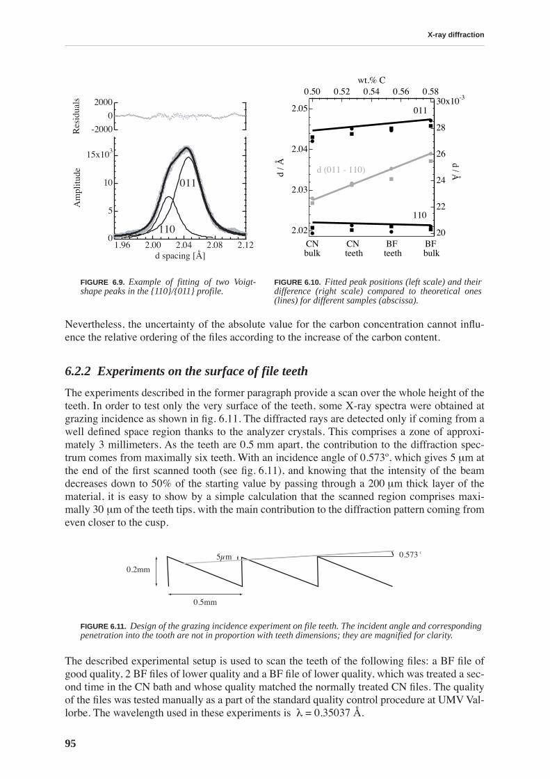
X-ray diffraction
95
Nevertheless, the uncertainty of the absolute value for the carbon concentration cannot influ-ence the relative ordering of the files according to the increase of the carbon content.
6.2.2 Experiments on the surface of file teeth
The experiments described in the former paragraph provide a scan over the whole height of theteeth. In order to test only the very surface of the teeth, some X-ray spectra were obtained atgrazing incidence as shown in fig. 6.11. The diffracted rays are detected only if coming from awell defined space region thanks to the analyzer crystals. This comprises a zone of approxi-mately 3 millimeters. As the teeth are 0.5 mm apart, the contribution to the diffraction spec-trum comes from maximally six teeth. With an incidence angle of 0.573º, which gives 5 µm atthe end of the first scanned tooth (see fig. 6.11), and knowing that the intensity of the beamdecreases down to 50% of the starting value by passing through a 200 µm thick layer of thematerial, it is easy to show by a simple calculation that the scanned region comprises maxi-mally 30 µm of the teeth tips, with the main contribution to the diffraction pattern coming fromeven closer to the cusp.
The described experimental setup is used to scan the teeth of the following files: a BF file ofgood quality, 2 BF files of lower quality and a BF file of lower quality, which was treated a sec-ond time in the CN bath and whose quality matched the normally treated CN files. The qualityof the files was tested manually as a part of the standard quality control procedure at UMV Val-lorbe. The wavelength used in these experiments is λ = 0.35037 Å.
FIGURE 6.9. Example of fitting of two Voigt-shape peaks in the {110}/{011} profile.
FIGURE 6.10. Fitted peak positions (left scale) and theirdifference (right scale) compared to theoretical ones(lines) for different samples (abscissa).
FIGURE 6.11. Design of the grazing incidence experiment on file teeth. The incident angle and correspondingpenetration into the tooth are not in proportion with teeth dimensions; they are magnified for clarity.
15x103
10
5
0
Am
plitu
de
2.122.082.042.001.96d spacing [Å]
-2000
0
2000
Res
idua
ls
110
011
2.05
2.04
2.03
2.02
d / Å
30x10-3
28
26
24
22
20
� d / Å
0.580.560.540.520.50wt.% C
BF bulk
BF teeth
CNbulk
CN teeth
011
110
d (011 - 110)
0.573 o5µm
0.2mm
0.5mm

Chapter 6
96
As seen from fig. 6.12, the resulting {110}/{011} martensite peaks differ in width. The twounsatisfactory BF files show the narrowest peaks, the peak for the good BF file is wider, andfor the additionally CN treated file the peak is widest and more asymmetric. The ordering ofthe files, going from the narrowest to the widest peak, corresponds to the ordering according toincreasing quality. As the peak width reflects the tetragonality, i.e. the amount of soluted car-bon, even remaining purely qualitative in the interpretation, it is possible to conclude that thequality of the files is related with the amount of carbon in solid solution at the very tips of thefile teeth.
The same relation in peak width is found for a pair of BF and CN treated files, which have beenaged at room temperature for 16.5 months (fig. 6.13). The measurements of TEP as a functionof aging time (figures 3.16 and 3.17) have already shown that although the difference in aver-age TEP between CN and BF treated files decreases with aging, the two groups of files are stillclearly distinguishable by TEP measurements. Therefore, it can be concluded that in the verysurface of the teeth tips, BF files have a lower concentration of soluted carbon than CN files.
The comparison of the {110}/{011} peak for the very surface of BF and CN treated files is ofgreat importance. It shows that the relation between BF and CN regarding carbon content isexactly the opposite at the very surface of the teeth than in the bulk. This is illustrated infig. 6.14. The X-ray diffraction spectra obtained from the file bulk (previously presented infig. 6.7 and 6.8) are transposed to the 2θ position for the wavelength λ = 0.35037 Å accordingto eq. 2.1, and compared with the spectra obtained from the teeth surface. It has to be notedthat the experiments on the bulk are made on different files, which were aged for almost a yearless. Figure 6.14 clearly illustrates that the peak broadening at the surface is smaller for BFfiles. The situation is the opposite in the bulk. The variation of the carbon concentration in thefile is indicated by the TEP measurement. Regarding X-ray diffraction results summarized infig. 6.14, it is possible to make a qualitative extension of TEP variation in the file profile pre-sented in fig. 3.22 to the teeth surface (fig. 6.15). The concentration of carbon decreases as theTEP increases: in the bulk of the files it is higher for the BF than for the CN treated files, and inthe teeth surface it is higher for the CN than for the BF treated files.
FIGURE 6.12. Peak {110}/{011} of the martensite fromthe tips of the file teeth for 2 bad BF files, one goodBF file and one bad BF file additionally treated in CNbath.
FIGURE 6.13. Peak {110}/{011} of the martensitefrom the tips of the file teeth for files aged at roomtemperature for more than one year.
3
15
10
5
Cou
nts
norm
aliz
ed
10.210.09.89.69.42θ [˚]
BF_bad1 BF_bad2 BF_good BF -> CN
3
15
10
5
Cou
nts
norm
aliz
ed
10.210.09.89.69.42θ [˚]
BF_bad1 BF_bad2 BF_good BF -> CN CN BF
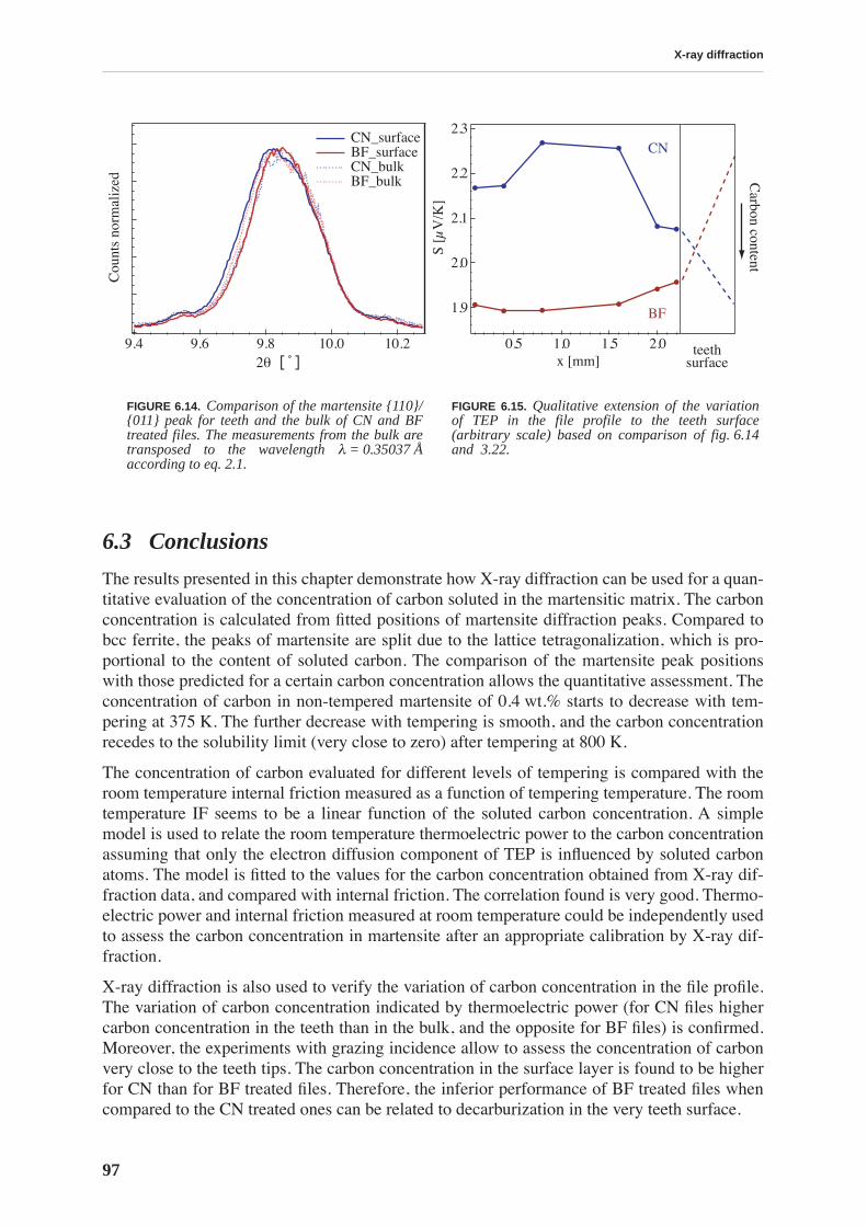
X-ray diffraction
97
6.3 Conclusions
The results presented in this chapter demonstrate how X-ray diffraction can be used for a quan-titative evaluation of the concentration of carbon soluted in the martensitic matrix. The carbonconcentration is calculated from fitted positions of martensite diffraction peaks. Compared tobcc ferrite, the peaks of martensite are split due to the lattice tetragonalization, which is pro-portional to the content of soluted carbon. The comparison of the martensite peak positionswith those predicted for a certain carbon concentration allows the quantitative assessment. Theconcentration of carbon in non-tempered martensite of 0.4 wt.% starts to decrease with tem-pering at 375 K. The further decrease with tempering is smooth, and the carbon concentrationrecedes to the solubility limit (very close to zero) after tempering at 800 K.
The concentration of carbon evaluated for different levels of tempering is compared with theroom temperature internal friction measured as a function of tempering temperature. The roomtemperature IF seems to be a linear function of the soluted carbon concentration. A simplemodel is used to relate the room temperature thermoelectric power to the carbon concentrationassuming that only the electron diffusion component of TEP is influenced by soluted carbonatoms. The model is fitted to the values for the carbon concentration obtained from X-ray dif-fraction data, and compared with internal friction. The correlation found is very good. Thermo-electric power and internal friction measured at room temperature could be independently usedto assess the carbon concentration in martensite after an appropriate calibration by X-ray dif-fraction.
X-ray diffraction is also used to verify the variation of carbon concentration in the file profile.The variation of carbon concentration indicated by thermoelectric power (for CN files highercarbon concentration in the teeth than in the bulk, and the opposite for BF files) is confirmed.Moreover, the experiments with grazing incidence allow to assess the concentration of carbonvery close to the teeth tips. The carbon concentration in the surface layer is found to be higherfor CN than for BF treated files. Therefore, the inferior performance of BF treated files whencompared to the CN treated ones can be related to decarburization in the very teeth surface.
FIGURE 6.14. Comparison of the martensite {110}/{011} peak for teeth and the bulk of CN and BFtreated files. The measurements from the bulk aretransposed to the wavelength λ = 0.35037 Åaccording to eq. 2.1.
FIGURE 6.15. Qualitative extension of the variationof TEP in the file profile to the teeth surface(arbitrary scale) based on comparison of fig. 6.14and 3.22.
3
8
6
4
2
0
Cou
nts
norm
aliz
ed
10.210.09.89.69.42θ [˚]
CN_surface BF_surface CN_bulk BF_bulk
2.3
2.2
2.1
2.0
1.9
S [µ
V/K
]
2.01.51.00.5x [mm]
BF
CN
surfaceteeth
Carbon content

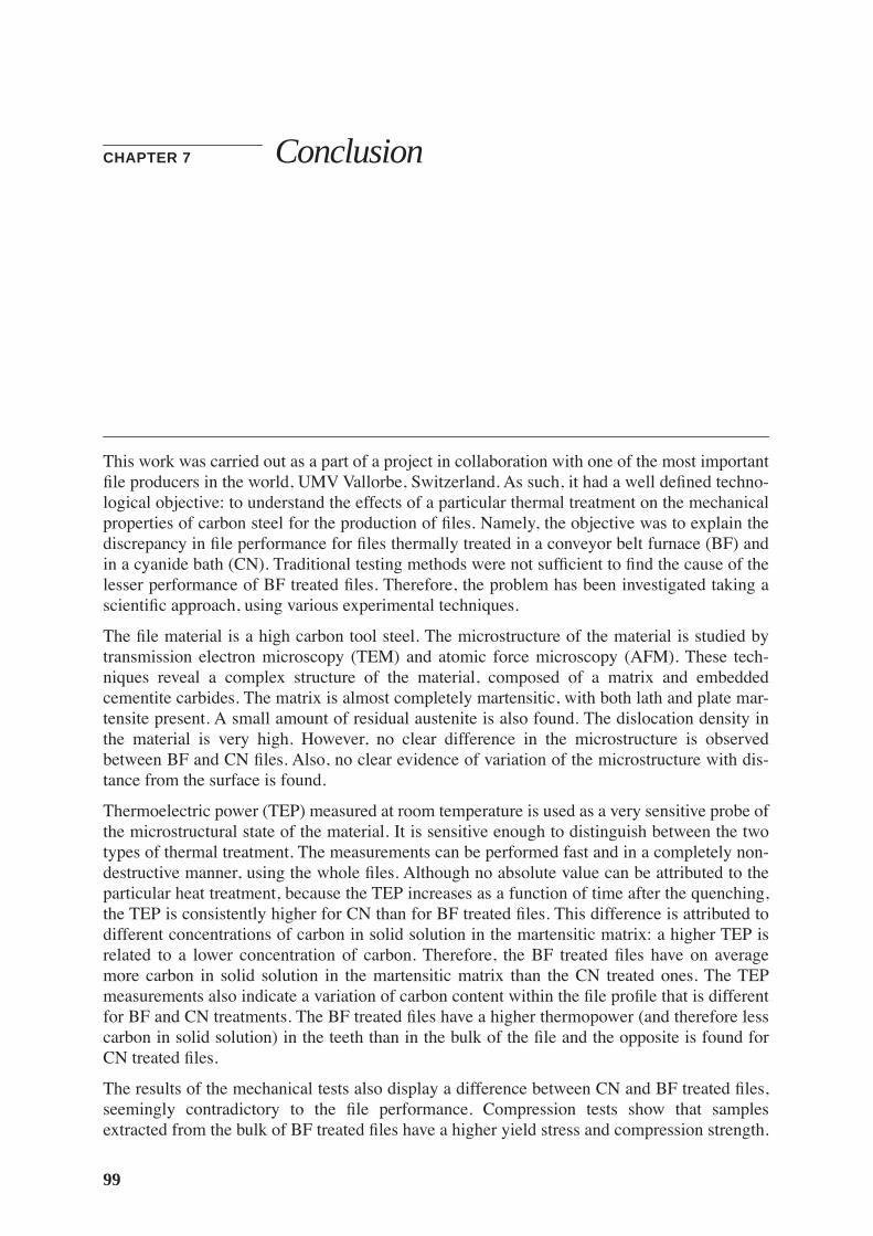
99
CHAPTER 7
Conclusion
This work was carried out as a part of a project in collaboration with one of the most importantfile producers in the world, UMV Vallorbe, Switzerland. As such, it had a well defined techno-logical objective: to understand the effects of a particular thermal treatment on the mechanicalproperties of carbon steel for the production of files. Namely, the objective was to explain thediscrepancy in file performance for files thermally treated in a conveyor belt furnace (BF) andin a cyanide bath (CN). Traditional testing methods were not sufficient to find the cause of thelesser performance of BF treated files. Therefore, the problem has been investigated taking ascientific approach, using various experimental techniques.
The file material is a high carbon tool steel. The microstructure of the material is studied bytransmission electron microscopy (TEM) and atomic force microscopy (AFM). These tech-niques reveal a complex structure of the material, composed of a matrix and embeddedcementite carbides. The matrix is almost completely martensitic, with both lath and plate mar-tensite present. A small amount of residual austenite is also found. The dislocation density inthe material is very high. However, no clear difference in the microstructure is observedbetween BF and CN files. Also, no clear evidence of variation of the microstructure with dis-tance from the surface is found.
Thermoelectric power (TEP) measured at room temperature is used as a very sensitive probe ofthe microstructural state of the material. It is sensitive enough to distinguish between the twotypes of thermal treatment. The measurements can be performed fast and in a completely non-destructive manner, using the whole files. Although no absolute value can be attributed to theparticular heat treatment, because the TEP increases as a function of time after the quenching,the TEP is consistently higher for CN than for BF treated files. This difference is attributed todifferent concentrations of carbon in solid solution in the martensitic matrix: a higher TEP isrelated to a lower concentration of carbon. Therefore, the BF treated files have on averagemore carbon in solid solution in the martensitic matrix than the CN treated ones. The TEPmeasurements also indicate a variation of carbon content within the file profile that is differentfor BF and CN treatments. The BF treated files have a higher thermopower (and therefore lesscarbon in solid solution) in the teeth than in the bulk of the file and the opposite is found forCN treated files.
The results of the mechanical tests also display a difference between CN and BF treated files,seemingly contradictory to the file performance. Compression tests show that samplesextracted from the bulk of BF treated files have a higher yield stress and compression strength.
Chapter 7
100
The hardness measured by nanoindentation is also found to be higher for the BF as comparedto the CN treated files. When compared to the TEP results, mechanical tests indicate that theresistance to deformation is proportional to the amount of carbon in solid solution.
Mechanical spectroscopy is used in order to study the micro-mechanical mechanisms responsi-ble for the macro-mechanical properties of the material. Namely, it is used to examine themobility of point defects and dislocations, and their interaction. It is found that significantaging occurs at room temperature shortly after quenching, and that the stabilized room temper-ature structure becomes again unstable with heating to temperatures higher than 375 K, caus-ing a decrease of IF and an increase of the elastic modulus. The martensitic structure ischaracterized by a rich internal friction temperature spectrum composed of five peaks (namedin increasing order) due to different relaxation and transition phenomena. The peak P1 is inter-preted as a Snoek-Köster hydrogen peak. A mechanism is proposed for the peak P2, involvingpipe-diffusion along kinks on screw dislocations. The peaks P3 and most likely also P4 are notrelaxation peaks. They are related to tempering effects that occur at temperatures higher than375 K. The peak P5 is interpreted as a Snoek-Köster carbon peak.
A small but significant difference between the IF spectra for the BF and CN treated materials isfound in very precise high frequency measurements: the internal friction is slightly higher forthe BF treated material. Upon heating, the difference becomes visible with the rise of the peakP2, and it continues to rise so that it is detectable also at room temperature. This difference isattributed to the existence of an athermal IF background proportional to the amount of carbonin solid solution. The background is related to long range dislocations - carbon interaction andthis is the first observation of such a mechanism in steel. This mechanism is also responsiblefor the increase of the IF observed for as quenched samples.
The tempering of the material indicated by the transition peaks in the internal friction measure-ments is studied combining several techniques. Differential scanning calorimetry reveals twostages of tempering. They are attributed to the precipitation of transition
η
-carbides and to thetransformation of residual austenite followed by precipitation of cementite, as confirmed byTEM observations. The recovery and recrystallization that occur at higher temperatures arealso observed by TEM. The tempering is reflected in an increase of thermoelectric power andYoung’s modulus, and by a decrease of hardness and internal friction. All mentioned physicalquantities start to change with the first stage of tempering observed around 375 K, whichimplies their sensitivity to soluted carbon. Their further evolution with tempering is somewhatdifferent, reflecting different sensitivity to other mechanisms. The hardness continuouslydecreases with tempering and no precipitation hardening is observed.
Finally, X-ray diffraction experiments allow quantification of the amount of carbon in solidsolution in the martensite. The carbon content is assessed from a comparison of the positionsof the martensite peaks in the X-ray diffraction spectra with the position calculated for differ-ent levels of lattice tetragonality, which is linearly dependent on carbon content. The concen-tration of carbon in non-tempered martensite of 0.4 wt.% starts to decrease with tempering at375 K. The further evolution of carbon concentration is smooth and the carbon content stabi-lizes at the solubility limit after tempering at 800 K.
The comparison of TEP, IF and X-ray diffraction results shows a strong correlation betweenthe carbon content and room temperature IF and TEP. A linear proportionality of IF to carboncontent is observed even in the absence of the carbon Snoek peak.
After demonstrating the applicability of X-ray diffraction to the determination of the evolutionof the carbon content with tempering, the method is used to verify the variation of carbon con-
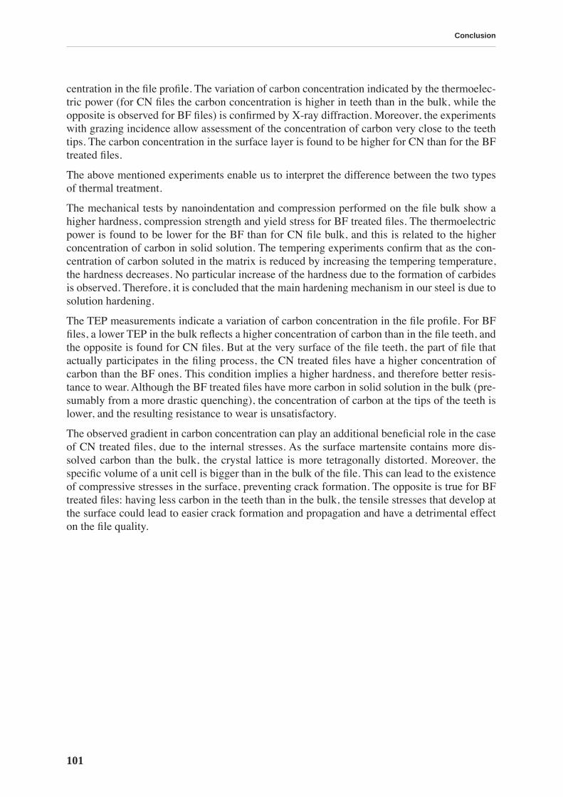
Conclusion
101
centration in the file profile. The variation of carbon concentration indicated by the thermoelec-tric power (for CN files the carbon concentration is higher in teeth than in the bulk, while theopposite is observed for BF files) is confirmed by X-ray diffraction. Moreover, the experimentswith grazing incidence allow assessment of the concentration of carbon very close to the teethtips. The carbon concentration in the surface layer is found to be higher for CN than for the BFtreated files.
The above mentioned experiments enable us to interpret the difference between the two typesof thermal treatment.
The mechanical tests by nanoindentation and compression performed on the file bulk show ahigher hardness, compression strength and yield stress for BF treated files. The thermoelectricpower is found to be lower for the BF than for CN file bulk, and this is related to the higherconcentration of carbon in solid solution. The tempering experiments confirm that as the con-centration of carbon soluted in the matrix is reduced by increasing the tempering temperature,the hardness decreases. No particular increase of the hardness due to the formation of carbidesis observed. Therefore, it is concluded that the main hardening mechanism in our steel is due tosolution hardening.
The TEP measurements indicate a variation of carbon concentration in the file profile. For BFfiles, a lower TEP in the bulk reflects a higher concentration of carbon than in the file teeth, andthe opposite is found for CN files. But at the very surface of the file teeth, the part of file thatactually participates in the filing process, the CN treated files have a higher concentration ofcarbon than the BF ones. This condition implies a higher hardness, and therefore better resis-tance to wear. Although the BF treated files have more carbon in solid solution in the bulk (pre-sumably from a more drastic quenching), the concentration of carbon at the tips of the teeth islower, and the resulting resistance to wear is unsatisfactory.
The observed gradient in carbon concentration can play an additional beneficial role in the caseof CN treated files, due to the internal stresses. As the surface martensite contains more dis-solved carbon than the bulk, the crystal lattice is more tetragonally distorted. Moreover, thespecific volume of a unit cell is bigger than in the bulk of the file. This can lead to the existenceof compressive stresses in the surface, preventing crack formation. The opposite is true for BFtreated files: having less carbon in the teeth than in the bulk, the tensile stresses that develop atthe surface could lead to easier crack formation and propagation and have a detrimental effecton the file quality.

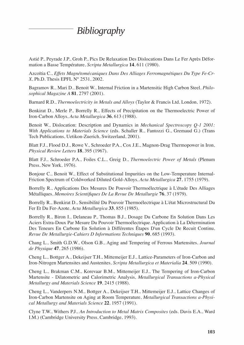
103
Bibliography
Astié P., Peyrade J.P., Groh P., Pics De Relaxation Des Dislocations Dans Le Fer Après Défor-mation a Basse Température,
Scripta Metallurgica
14
, 611 (1980).
Azcoïtia C.,
Effets Magnétomécaniques Dans Des Alliages Ferromagnétiques Du Type Fe-Cr-X
, Ph.D. Thesis EPFL N° 2531, 2002.
Bagramov R., Mari D., Benoit W., Internal Friction in a Martensitic High Carbon Steel,
Philo-sophical Magazine A
81
, 2797 (2001).
Barnard R.D.,
Thermoelectricity in Metals and Alloys
(Taylor & Francis Ltd, London, 1972).
Benkirat D., Merle P., Borrelly R., Effects of Precipitation on the Thermoelectric Power ofIron-Carbon Alloys,
Acta Metallurgica
36
, 613 (1988).
Benoit W., Dislocation: Description and Dynamics in
Mechanical Spectroscopy Q-1 2001:With Applications to Materials Science
(eds. Schaller R., Fantozzi G., Gremaud G.) (TransTech Publications, Uetikon-Zuerich, Switzerland, 2001).
Blatt F.J., Flood D.J., Rowe V., Schroeder P.A., Cox J.E., Magnon-Drag Thermopower in Iron,
Physical Review Letters
18
, 395 (1967).
Blatt F.J., Schroeder P.A., Foiles C.L., Greig D.,
Thermoelectric Power of Metals
(PlenumPress, New York, 1976).
Bonjour C., Benoit W., Effect of Substitutional Impurities on the Low-Temperature Internal-Friction Spectrum of Coldworked Diluted Gold-Alloys,
Acta Metallurgica
27
, 1755 (1979).
Borrelly R., Applications Des Mesures De Pouvoir Thermoélectrique à L'étude Des AlliagesMétalliques,
Memoires Scientifiques De La Revue De Metallurgie
76
, 37 (1979).
Borrelly R., Benkirat D., Sensibilité Du Pouvoir Thermoélectrique à L'état Microstructural DuFer Et Du Fer-Azote,
Acta Metallurgica
33
, 855 (1985).
Borrelly R., Biron I., Delaneau P., Thomas B.J., Dosage Du Carbone En Solution Dans LesAciers Extra-Doux Par Mesure Du Pouvoir Thermoélectrique. Application à La DéterminationDes Teneurs En Carbone En Solution à Différentes Étapes D'un Cycle De Recuit Continu,
Revue De Metallurgie-Cahiers D Informations Techniques
90
, 685 (1993).
Chang L., Smith G.D.W., Olson G.B., Aging and Tempering of Ferrous Martensites,
Journalde Physique
47
, 265 (1986).
Cheng L., Bottger A., Dekeijser T.H., Mittemeijer E.J., Lattice-Parameters of Iron-Carbon andIron-Nitrogen Martensites and Austenites,
Scripta Metallurgica et Materialia
24
, 509 (1990).
Cheng L., Brakman C.M., Korevaar B.M., Mittemeijer E.J., The Tempering of Iron-CarbonMartensite - Dilatometric and Calorimetric Analysis,
Metallurgical Transactions a-PhysicalMetallurgy and Materials Science
19
, 2415 (1988).
Cheng L., Vanderpers N.M., Bottger A., Dekeijser T.H., Mittemeijer E.J., Lattice Changes ofIron-Carbon Martensite on Aging at Room Temperature,
Metallurgical Transactions a-Physi-cal Metallurgy and Materials Science
22
, 1957 (1991).
Clyne T.W., Withers P.J.,
An Introduction to Metal Matrix Composites
(eds. Davis E.A., WardI.M.) (Cambridge University Press, Cambridge, 1993).
Bibliography
104
Cohen M., The Strengthening of Steel,
Transactions of the Metallurgical Society of AIME
224
,638 (1962).
Eshelby J.D., The Determination of the Elastic Field of an Ellipsoidal Inclusion, and RelatedProblems,
Proc. R. Soc.
241A
, 376 (1957).
Fornerod R.,
Un Phénomène D'interaction Entre Défauts D'irradiation Et Dislocations DansL'argent Polycristallin
, Ph.D. Thesis EPFL N° 70, 1968.
Fuoss R.M., Kirkwood J.G., Electrical Properties of Solids. Viii. Dipole Moments in PolyvinylChloride-Diphenyl Systems,
Journal of the American Chemical Society
63
, 385 (1941).
Ghosh G., Olson G.B., The Isotropic Shear Modulus of Multicomponent Fe-Base Solid Solu-tions,
Acta Materialia
50
, 2655 (2002).
Gremaud G., Dislocation - Point Defect Interactions in
Mechanical Spectroscopy Q-1 2001:With Applications to Materials Science
(eds. Schaller R., Fantozzi G., Gremaud G.) (TransTech Publications, Uetikon-Zuerich, Switzerland, 2001).
Gremaud G., Kustov S., Theory of Dislocation-Solute Atom Interactions in Solid Solutionsand Related Nonlinear Anelasticity,
Physical Review B
60
, 9353 (1999).
Han K., Van Genderen M.J., Bottger A., Zandbergen H.W., Mittemeijer E.J., Initial Stages ofFe-C Martensite Decomposition,
Philosophical Magazine a-Physics of Condensed MatterStructure Defects and Mechanical Properties
81
, 741 (2001).
Honeycombe R.,
Steels; Microstructure and Properties
(ed. R. Honeycombe P.H.) (1980).
Inoue T., Haraguchi K., Kimura S., Analysis of Stresses Due to Quenching and Tempering ofSteel,
Transactions of the Iron and Steel Institute of Japan
18
, 11 (1978).
Isoré A.,
Etude De La Recristallisation Primaire De L’argent Par Mesures De FrottementIntérieur Et De Défaut De Module
, Ph.D. Thesis EPFL N° 159, 1973.
Johnson R.A., Calculation of the Energy and Migration Characteristics of Carbon in Marten-site,
Acta Metallurgica
13
, 1239 (1965).
Kamber K., Keefer D., Wert C., Interactions of Interstitials with Dislocations in Iron,
Acta Met-allurgica
9
, 403 (1961).
Kis A.,
Mechanical Properties of Mesoscopic Objects
, Ph.D. Thesis EPFL N° 2876, 2003.
Klems G.J., Miner R.E., Hultgren F.A., Gibala R., Internal Friction in Ferrous Martensites,
Metallurgical Transactions A
7
, 839 (1976).
Krauss G., Tempering and Structural Changes in Ferrous Martensites in
Phase Transforma-tions in Ferrous Alloys
(eds. Mader A.R., Goldstein J.I.) (The Metallurgical Society, 1984).
Kurdjumov G.V., Martensite Crystal Lattice, Mechanism of Austenite-Martensite Transforma-tion and Behavior of Carbon Atoms in Martensite,
Metallurgical Transactions A
7A
, 999(1976).
Kustov S., Gremaud G., Benoit W., Golyandin S., Sapozhnikov K., Nishino Y., Asano S.,Strain Amplitude-Dependent Anelasticity in Cu-Ni Solid Solution Due to Thermally Activatedand Athermal Dislocation-Point Obstacle Interactions,
Journal of Applied Physics
85
, 1444(1999).
Languillaume J., Kapelski G., Baudelet B., Cementite Dissolution in Heavily Cold DrawnPearlitic Steel Wires,
Acta Materialia
45
, 1201 (1997).
Bibliography
105
Lavaire N., Massardier V., Merlin J., Quantitative Evaluation of the Interstitial Content (C and/or N) in Solid Solution in Extra-Mild Steels by Thermoelectric Power Measurements,
ScriptaMaterialia
50
, 131 (2004).
Mercier O.,
Effets des impuretés sur le spectre et la restauration des pics de Hasiguti de l’orécroui ou irradié
, Ph.D. Thesis EPFL N° 180, 1974.
MacDonald D.K.C.,
Thermoelectricity: An Introduction to the Principles
(John Wiley & Sons,New York, London, 1962).
Maddin R., A History of Martensite: Some Thoughts on the Early Hardening of Iron in
Mar-tensite
(eds. Olson G.B., Owen W.S.) (ASM International, USA, 1992).
Magalas L.B., Dufresne J.F., Moser P., The Snoek-Köster Relaxation in Iron,
Journal de Phy-sique
42
, 127 (1981).
Mari D., Bolognini S., Feusier G., Viatte T., Benoit W., Experimental Strategy to Study theMechanical Behaviour of Hardmetals for Cutting Tools,
International Journal of RefractoryMetals & Hard Materials
17
, 209 (1999).
Massardier V., Lavaire N., Soler M., Merlin J., Comparison of the Evaluation of the CarbonContent in Solid Solution in Extra-Mild Steels by Thermoelectric Power and by Internal Fric-tion,
Scripta Materialia
50
, 1435 (2004).
Mittemeijer E.J., Analysis of the Kinetics of Phase-Transformations,
Journal of Materials Sci-ence
27
, 3977 (1992).
Mittemeijer E.J., Wierszyllowski I.A., The Isothermal and Nonisothermal Kinetics of Temper-ing Iron-Carbon and Iron-Nitrogen Martensites and Austenites,
Zeitschrift für Metallkunde
82
,419 (1991).
Moss S.C., Static Atomic Displacements in Iron-Carbon Martensite,
Acta Metallurgica
15
,1815 (1967).
Mura T., Tamura I., Brittain J.O., On the Internal Friction of Cold-Worked and Quenched Mar-tensitic Iron and Steel,
Journal of Applied Physics
32
, 92 (1961).
Nishiyama Z.,
Martensitic Transformation
(Academic Press, New York, 1978).
Nowick A.S., Berry B.S.,
Anelastic Relaxation in Crystalline Solids
(Academic Press, NewYork, 1972a).
Nowick A.S., Berry B.S., The High-Temperature Background in
Anelastic Relaxation in Crys-talline Solids
(Academic Press, New York, 1972b).
Numakura H., Koiwa M., The Snoek Relaxation in Dilute Ternary Alloys. A Review,
Journalde Physique IV
6
, C8 (1996).
Ohmori Y., Tamura I., Epsilon Carbide Precipitation During Tempering of Plain Carbon Mar-tensite,
Metallurgical Transactions a-Physical Metallurgy and Materials Science
23
, 2737(1992).
Oliver W.C., Phar G.M., An Improved Technique for Determining Hardness and Elastic-Modu-lus Using Load and Displacement Sensing Indentation Experiments,
Journal of MaterialsResearch
7
, 1564 (1992).
Olson G.B., Introduction: Martensite in Perspective in
Martensite
(eds. Olson G.B., OwenW.S.) (ASM International, USA, 1992).
Bibliography
106
Olson G.B., Cohen M., Early Stages of Aging and Tempering of Ferrous Martensites, Metal-lurgical Transactions a-Physical Metallurgy and Materials Science 14, 1057 (1983).
Owen W.S., The Strength of Ferrous Martensite in Martensite (eds. Olson G.B., Owen W.S.)(ASM International, 1992).
Parke S., Logarithmic Decrements at High Damping, British Journal of Applied Physics 17,271 (1966).
Petarra D.P., Beshers D.N., Cold-Work Internal Friction Peak in Iron, Acta Metallurgica 15,791 (1967).
Rodriguez C.A.V.D.A., Prioul C., Hyspecka L., Isothermal Martensitic Transformation in Fe-Ni and Fe-Ni-C Alloys at Subzero Temperatures, Metallurgical Transactions A 15, 2193(1984).
Rose A., Hougardy H., Atlas Zur Wärmebehandlung Der Stähle (Verlag Stahleisen m.b.H.,Dèsseldorf, 1972).
Saitoh H., Yoshinaga N., Ushioda K., Influence of Substitutional Atoms on the Snoek Peak ofCarbon in B.C.C. Iron, Acta Materialia 52, 1255 (2004).
Samuel F.H., Hussein A.A., A Comparative-Study of Tempering in Steel, Materials Scienceand Engineering 58, 113 (1983).
San juan J., Fantozzi G., No M.L., Esnouf C., Hydrogen Snoek-Köster Relaxation in Iron,Journal of Physics F: Metal Physics 17, 837 (1987a).
San juan J., Fantozzi G., No M.L., Esnouf C., Vanoni F., Analysis of Snoek-Köster (H) Relax-ation in Iron, Journal de Physique 46, C10 (1985).
San juan J., No M.L., Fantozzi G., Esnouf C., Experimental-Evidence of Relaxation Arisingfrom the Motion of Geometrical Kinks on Screw Dislocations in Iron, Philosophical MagazineLetters 56, 237 (1987b).
Schaller R., Fantozzi G., Gremaud G. (eds.), Mechanical Spectroscopy Q-1 2001: With Appli-cations to Materials Science (Trans Tech Publications, Uetikon-Zuerich, Switzerland, 2001).
Schmidtmann E., Hougardy H., Schenk H., Investigation of the Decomposition of Martensitein the First Stage of Tempering by Measuring Elasticity Modulus and Damping at High Fre-quencies, Archiv für das Eisenhüttenwesen 36, 191 (1965).
Schultz H., Defect Parameters of B.C.C. Metals: Group Specific Trends, Materials Science andEngineering A141, 149 (1991).
Seeger A., A Theory of the Snoek-Köster Relaxation (Cold-Work Peak) in Metals, PhysicaStatus Solidi. Section A. Applied Research 55, 457 (1979).
Seeger A., Wüthrich C., Dislocation Relation Processes in Body-Centred Cubic Materials, IlNuovo Cimento 33B, 39 (1976).
Snoek J.L., Physica 6, 591 (1939).
Speich G.R., Tempering of Low-Carbon Martensite, Transactions of the Metallurgical Societyof AIME 245, 2553 (1969).
Speich G.R., Leslie W.C., Tempering of Steel, Metallurgical Transactions 3, 1043 (1972a).
Speich G.R., Leslie W.C., Elastic-Constants of Martensite, Metallurgical Transactions 4, 1873(1973).
Bibliography
107
Speich G.R., Schwoebl.Aj, Leslie W.C., Elastic-Constants of Binary Iron-Base Alloys, Metal-lurgical Transactions 3, 2031 (1972b).
Speich G.R., Taylor K., Tempering of Ferrous Martensites in Martensite (eds. Olson G.B.,Owen W.S.) (ASM International, 1992).
Stark P., Averbach B.L., Cohen M., Internal Friction Measurements on Tempered Martensite,Acta Metallurgica 4, 91 (1956).
Stark P., Averbach B.L., Cohen M., Influence of Microstructure on the Carbon Damping Peakin Iron-Carbon Alloys, Acta Metallurgica 6, 149 (1958).
Taniyama A., Takayama T., Arai M., Hamada T., Structure Analysis of Ferrite in DeformedPearlitic Steel by Means of X-Ray Diffraction Method with Synchrotron Radiation, ScriptaMaterialia 51, 53 (2004).
Timoshenko S., Résistance Des Matériaux (Librarie Polytechnique Béranger, Paris, 1963).
Tkalcec I., Mari D., Mechanical Spectroscopy in Martensitic and Cold-Worked Carbon Steels,Defects and Diffusion in Metals: An Annual Retrospective Iv 203-205, 253 (2002).
Umemoto M., Liu Z.G., Masuyama K., Tsuchiya K., Influence of Alloy Additions on Produc-tion and Properties of Bulk Cementite, Scripta Materialia 45, 391 (2001).
Van Genderen M.J., Bottger A., Cernik R.J., Mittemeijer E.J., Early Stages of Decompositionin Iron-Carbon and Iron-Nitrogen Martensites - Diffraction Analysis Using Synchrotron-Radi-ation, Metallurgical Transactions a-Physical Metallurgy and Materials Science 24, 1965(1993).
Van Genderen M.J., Isac M., Böttger A., Mittemeijer E.J., Aging and Tempering Behavior ofIron-Nickel-Carbon and Iron-Carbon Martensite, Metallurgical and Materials Transactions a-Physical Metallurgy and Materials Science 28, 545 (1997).
Vincent A., Réalisation D'un Ensamble De Mesures Ultrasonores; Application à L'étude DesDéfauts Cristallins Dans L'aluminium, Ph.D. Thesis, Universite Claude Bernard de Lyon,1973.
Vittoz B., Secrétan B., Martinet B., Frottement Interne Et Anélasticité Des Solides, Zeitschriftfür Angewandte Mathematik und Physik 14, 46 (1963).
Ward R., Capus J.M., Internal Friction Effects in Martensite, Journal of the Iron and SteelInstitute 201, 1038 (1963).
Weller M., The Snoek-Köster Relaxation in Body-Centred Cubic Metals, Journal de Physique44, C9 (1983).
Weller M., Anelastic Relaxation of Point Defects in Cubic Crystals, Journal de Physique IV 6,C8 (1996).
Weller M., Point Defect Relaxations in Mechanical Spectroscopy Q-1 2001: With Applicationsto Materials Science (eds. Schaller R., Fantozzi G., Gremaud G.) (Trans Tech Publications,Uetikon-Zuerich, Switzerland, 2001).
Wenzl H., Welter J.M., Electric Transport Properties of High-Purity Metals and Influence ofTrace Impurities, Zeitschrift für Metallkunde 65, 205 (1974).
Zener C., Mechanical Behavior of High Damping Metals, Journal of Applied Physics 18, 1022(1947).
Zener C., Elasticity and Anelasticity of Metals (Chicago University Press, Chicago, 1948).


103
Acknowledgments
It is a pleasure to thank the many people who made this thesis possible.
I am most grateful to my thesis director, Prof. Willy Benoit, for accepting me into his groupand allowing me to work in such excellent conditions. But above all, I am thankful for his kind-ness, guidance, support and encouragement.
It would be difficult to overstate my gratitude to Daniele Mari who followed and guided mywork closely. With his expertise, inspiration and endless optimism he helped me find my way.
I wish to thank Robert Schaller for passing onto me a little of his expertise and enthusiasmabout mechanical spectroscopy, and Gérard Gremaud for helpful theoretical discussions andideas. Many thanks must also go to Sybille Crevoiserat and Christian Azcoïtia for the TEMimages, and to Hermann Emerich and Wouter van Beek for their help with X-ray diffractionmeasurements at ESRF.
This work has been achieved in collaboration with UMV Vallorbe, Switzerland. I am gratefulto Bruno Jouan, Géraldine Marlin and Marc Christen for the excellent contact I have had withthem over the past four years and for their confidence in my work.
My measurements would not have been possible without careful sample preparation, for whichI thank Antonio Gentile, Guillaume Camarda and especially Gérald Beney for spark-cuttingand polishing to perfection.
I thank Bernard Guisolan for fixing everything that I broke, Alessandro Ichino for his humorand many electronics repairs and Philippe Bugnon for his help and whistling.
I owe a debt of gratitude to many doctorants, ex-doctorants and collaborators, who helped mewhen my French was at level zero, assisted me both at work and elsewhere, and who most ofall made the atmosphere at EPFL really enjoyable. I would particularly like to thank KatharinaBuß and Patrick Mayor who shared with me so much more than just the office and who werenot only my colleagues, but true friends.
I am indebted to Ana Smontara and Prof. László Forró for inspiring me to do my Ph.D. in Lau-sanne.
Immense thanks to my big family, who let me go so far from them. I thank them for all theirlove and support.
And I thank Marko for driving me 6000 km and for fig. 3.21. And for everything else.

Curriculum vitae
Iva Tkalcec
born on January 27th, 1974 in Zagreb, Croatia
nationality: Croatian
Education:
2000-2004: Ph.D. student at EPF Lausanne, Faculty of Basic Sciences, Institute of Physicsof Complex Matter under supervision of Dr. D. Mari and thesis director Prof. W.Benoit
2000: Diploma work “Anisotropy of thermal conductivity of (TaSe4)2I”, performed atInstitute of Physics, Zagreb, Croatia
1992-2000: Physics at University of Zagreb, Faculty of Science, Croatia
1992: V Gimnazija, Zagreb, Croatia
Teaching:
2003: Assistant for “Introduction à la Métrologie”, with G. Gremaud and R. Schaller
2000-2003: Assistant for “Travaux pratiques des physiciens de 2eme année”, with G. Gre-maud
2000: Assistant for “Travaux pratiques de Physique destinés aux étudiants des sectionsde Mécanique et de Microtechnique”, with R. Sanjines
Conferences:
2003: I. Tkalcec, C. Azcoïtia, S. Crevoiserat, D. Mari: “Tempering effects on a mar-tensitic high carbon steel”, oral presentation, 13th International Conference onthe Strength of Materials, Budapest, Hungary
I. Tkalcec, C. Azcoïtia, D. Mari: “Tempering effects on the microstructure ofmartensitic carbon steel”, oral presentation, Annual meeting of the Swiss Physi-cal Society, Basel, Switzerland
2002: I. Tkalcec, S. Crevoiserat, D. Mari: “Interaction between dislocations and pointdefects in martensitic carbon steels”, poster, NATO Advanced Study Institute:Thermodynamics, Microstructures and Plasticity, Fréjus, France
I. Tkalcec and D. Mari: “Internal friction in martensitic, ferritic and bainitic car-bon steel; cold work effects”, oral presentation, 13th International Conferenceon Internal Friction and Ultrasonic Attenuation in Solids, Bilbao, Spain
I. Tkalcec, S. Crevoiserat, D. Mari: “Interaction between dislocations and pointdefects in martensitic carbon steels”, poster, Colloque Plasticité 2002, Lyon,France
Thermoelectric Phenomena in Metals and Alloys, workshop, INSA Lyon,France
2001: I. Tkalcec and D. Mari: “Mechanical spectroscopy in a martensitic carbonsteel”, poster, Mechanical spectroscopy Q-1, summer school, Aussois, France
Publications:
I. Tkalcec, C. Azcoïtia, S. Crevoiserat, D. Mari: “Tempering effects on a mar-tensitic high carbon steel”, Materials Science and Engineering A, In Press, Cor-rected Proof, Available online 26 June 2004
I. Tkalcec, D. Mari: “Internal friction in martensitic, ferritic and bainitic carbonsteel; cold work effects”, Materials Science and Engineering A 370 (1-2), 213-217 (2004)
I. Tkalcec, D. Mari: “Mechanical Spectroscopy in Martensitic and Cold-WorkedCarbon Steels”, Defect and Diffusion Forum Vols. 203-205, pp. 253-256 (2002)
A. Smontara, I. Tkalcec, A. Bilusic, M. Budimir, H. Berger: “Anisotropy of thethermal conductivity in (TaSe4)2 I”, Physica B 316 (2002) pp. 279-282
I. Tkalcec, A. Bilusic, H. Berger, L. Forro, A. Smontara: “Anisotropy of thetransport properties of (TaSe4)2 I”, Synthetic Metals 120 (1-3): 883-884 Sp. Iss.SI MAR 15 (2001)
I. Tkalcec, A. Bilusic, H. Berger, L. Forro, A. Smontara: Anisotropic thermo-electric properties of (TaSe4)2 I”, Fizika A 9 (2000) 4, 169-176