i

Mechanical Properties of Polycrystalline Ceramics by Nanoindentation Methods: Effect

of Surface Roughness and Tip Size

A Thesis

Submitted to the Faculty

of

Drexel University

by

Ismail C. Albayrak

in partial fulfillment of the

requirements for the degree

of

Master of Science

in

Materials Science and Engineering

December 2009

ii

© Copyright 2009 Ismail C. Albayrak. All Rights Reserved.

iii

Dedication

This thesis is dedicated to my father (Ahmet Albayrak), mother (Meral Albayrak), and

brother (Adil Cem Albayrak), who supported and inspired me at the every moment of my

life.

iv

Acknowledgments

I would like thank everyone who helped me or supported me in a way during my education at

Drexel University.

First I would like to thank Prof. Michel W. Barsoum with all of my heart for his supervising

and unlimited help anytime during my education. He believed and supported me even at the

times I was losing my ambition. I could not finish this work without his support. I would also

like to thank my co-advisor Prof. Ori Yeheskel because of his mentorship, encouragement

and endless inspiration to me. During his visiting time at Drexel University, I learned a lot

from him, and I am still learning. I cannot even find words to thank enough to both of them.

I am very grateful to my thesis committee members Prof. Antonios Zavaliangos, Prof. Steven

May and Prof. Yury Gogotsi for their precious time and evaluation of my research. I also

want to thank all of the faculty member and staff in the Materials Science and Engineering

Department of Drexel University.

I would specially like to thank Dr. Sandip Basu for especially his great help with

nanoindentation. He was a perfect mentor who I learned so much from. I would also like to

thank MAX research group members - Dr. Aaron Sakulich, Dr. Aiguo Zhou, Mr. Alexander

J. Moseson, Mr. Babak Anasori, Mr. Charles Spencer Jr., Mr. Darin Tallman, Mr. Eric

Eisele, Miss. Eshani Sarma, Dr. Eva Jud Sierra, Mr. John Lloyd, Mr. Mohammed Shamma,

v

Miss. Nina J. Lane, Mr. Sean Miller, Dr. Shahram Amini, Mr. Theodore Scabarozi Jr. and

Dr. Youngsoo Chung - for their invaluable help and support since the beginning. It was a

great pleasure and honor to be a part of the same research group with them.

I also want to thank my friends in my office and in the department - Mrs. Amalie Oroho,

Miss. Amanda Levinson, Mr. Christopher Winkler, Mr. Ioannis Neitzel, Mr. Jerry Klinzing,

Mr. Matthew Hood, Mr. Min Heon, Mr. Murat E. Kurtoğlu, Mr. Philipp Hunger, Mr. Taha

Demirkan, Mrs. Valerie Binetti, Mr. Veli Kara and the ones I could not remember – for their

friendship and making the office and the labs always fun to work in. I am so glad to meet

them. Before I forget, I want to express my thanks to my roommates Mr. Gary Bryla, Miss.

Mary Long, Miss. Monica Fonorow and Mr. Michael J. Sexton for being a family for me in

my stay here and making my every day enjoyable.

Last but not least, I would like to thank my parents and my brother. I could not complete this

work without their priceless love, support and motivation.

This work was supported by Republic of Turkey - The Ministry of National Education.

vi

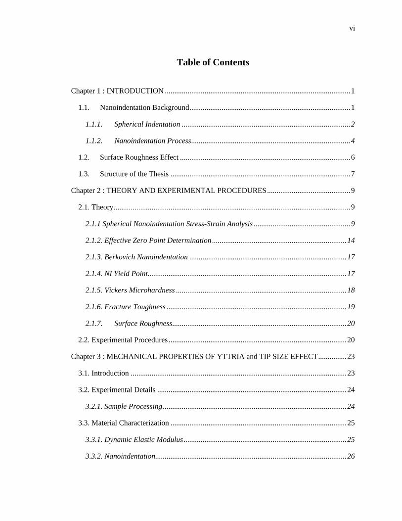
Table of Contents

Chapter 1 : INTRODUCTION .................................................................................................. 1

1.1. Nanoindentation Background ..................................................................................... 1

1.1.1. Spherical Indentation ......................................................................................... 2

1.1.2. Nanoindentation Process .................................................................................... 4

1.2. Surface Roughness Effect .......................................................................................... 6

1.3. Structure of the Thesis ............................................................................................... 7

Chapter 2 : THEORY AND EXPERIMENTAL PROCEDURES ............................................ 9

2.1. Theory ............................................................................................................................. 9

2.1.1 Spherical Nanoindentation Stress-Strain Analysis ................................................... 9

2.1.2. Effective Zero Point Determination ....................................................................... 14

2.1.3. Berkovich Nanoindentation ................................................................................... 17

2.1.4. NI Yield Point ......................................................................................................... 17

2.1.5. Vickers Microhardness .......................................................................................... 18

2.1.6. Fracture Toughness ............................................................................................... 19

2.1.7. Surface Roughness ............................................................................................ 20

2.2. Experimental Procedures .............................................................................................. 20

Chapter 3 : MECHANICAL PROPERTIES OF YTTRIA and TIP SIZE EFFECT ............... 23

3.1. Introduction .................................................................................................................. 23

3.2. Experimental Details .................................................................................................... 24

3.2.1. Sample Processing ................................................................................................. 24

3.3. Material Characterization ............................................................................................. 25

3.3.1. Dynamic Elastic Modulus ...................................................................................... 25

3.3.2. Nanoindentation ..................................................................................................... 26

vii

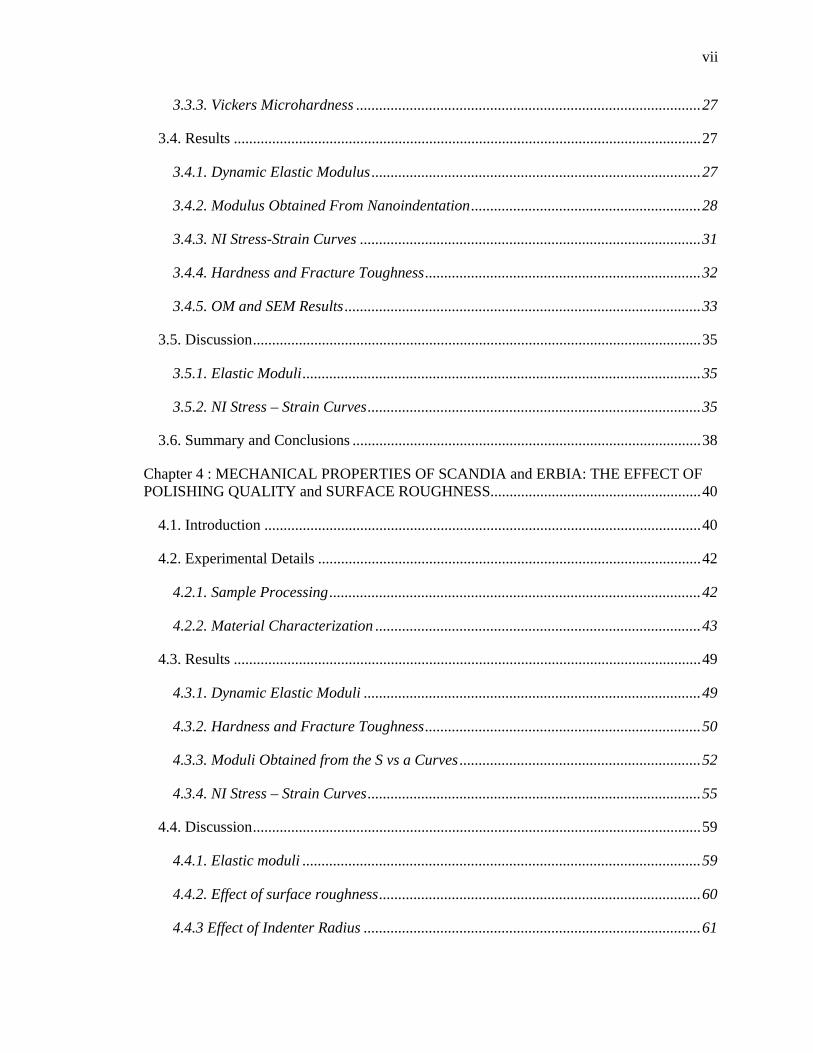
3.3.3. Vickers Microhardness .......................................................................................... 27

3.4. Results .......................................................................................................................... 27

3.4.1. Dynamic Elastic Modulus ...................................................................................... 27

3.4.2. Modulus Obtained From Nanoindentation ............................................................ 28

3.4.3. NI Stress-Strain Curves ......................................................................................... 31

3.4.4. Hardness and Fracture Toughness ........................................................................ 32

3.4.5. OM and SEM Results ............................................................................................. 33

3.5. Discussion ..................................................................................................................... 35

3.5.1. Elastic Moduli ........................................................................................................ 35

3.5.2. NI Stress – Strain Curves ....................................................................................... 35

3.6. Summary and Conclusions ........................................................................................... 38

Chapter 4 : MECHANICAL PROPERTIES OF SCANDIA and ERBIA: THE EFFECT OF POLISHING QUALITY and SURFACE ROUGHNESS....................................................... 40

4.1. Introduction .................................................................................................................. 40

4.2. Experimental Details .................................................................................................... 42

4.2.1. Sample Processing ................................................................................................. 42

4.2.2. Material Characterization ..................................................................................... 43

4.3. Results .......................................................................................................................... 49

4.3.1. Dynamic Elastic Moduli ........................................................................................ 49

4.3.2. Hardness and Fracture Toughness ........................................................................ 50

4.3.3. Moduli Obtained from the S vs a Curves ............................................................... 52

4.3.4. NI Stress – Strain Curves ....................................................................................... 55

4.4. Discussion ..................................................................................................................... 59

4.4.1. Elastic moduli ........................................................................................................ 59

4.4.2. Effect of surface roughness .................................................................................... 60

4.4.3 Effect of Indenter Radius ........................................................................................ 61

viii

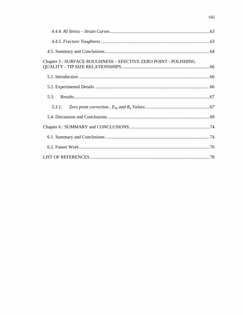
4.4.4. NI Stress – Strain Curves ....................................................................................... 63

4.4.5. Fracture Toughness ............................................................................................... 63

4.5. Summary and Conclusions ........................................................................................... 64

Chapter 5 : SURFACE ROUGHNESS – EFECTIVE ZERO POINT - POLISHING QUALITY - TIP SIZE RELATIONSHIPS ............................................................................. 66

5.1. Introduction .................................................................................................................. 66

5.2. Experimental Details .................................................................................................... 66

5.3. Results ...................................................................................................................... 67

5.3.1. Zero point correction , ESp and Rq Values ........................................................ 67

5.4. Discussion and Conclusions ......................................................................................... 69

Chapter 6 : SUMMARY and CONCLUSIONS ...................................................................... 74

6.1. Summary and Conclusions ........................................................................................... 74

6.2. Future Work .................................................................................................................. 76

LIST OF REFERENCES ........................................................................................................ 78

ix

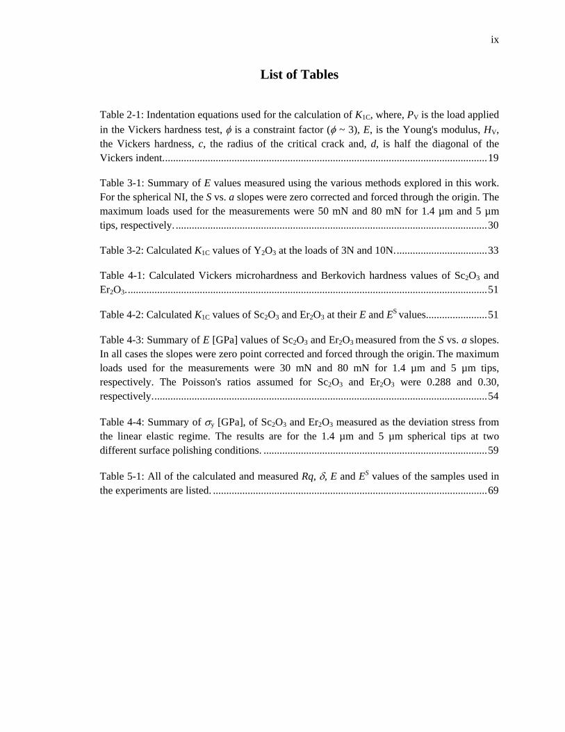
List of Tables

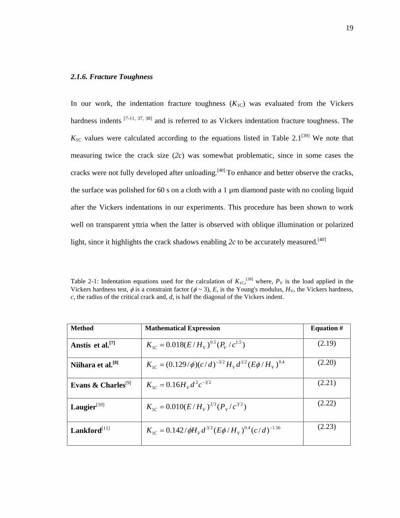
Table 2-1: Indentation equations used for the calculation of K1C, where, PV is the load applied in the Vickers hardness test, φ is a constraint factor (φ ~ 3), E, is the Young's modulus, HV, the Vickers hardness, c, the radius of the critical crack and, d, is half the diagonal of the Vickers indent. ......................................................................................................................... 19

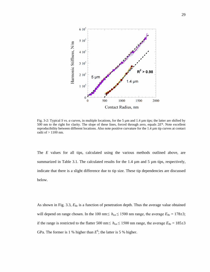
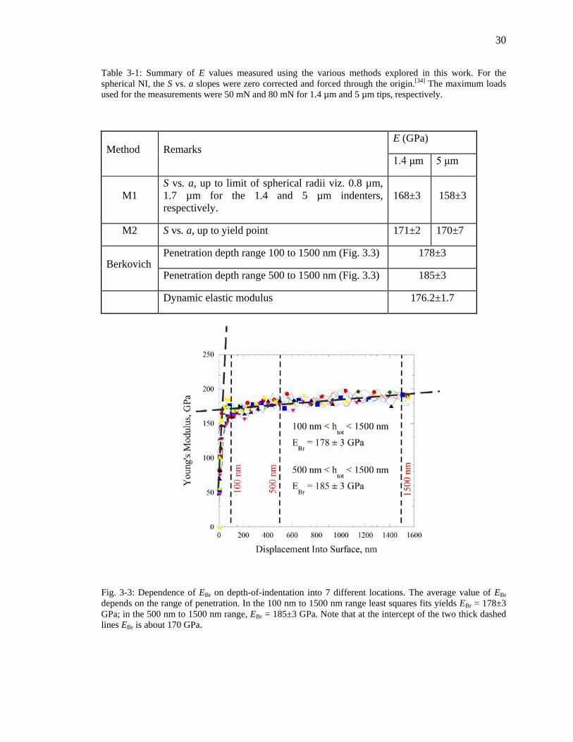
Table 3-1: Summary of E values measured using the various methods explored in this work. For the spherical NI, the S vs. a slopes were zero corrected and forced through the origin. The maximum loads used for the measurements were 50 mN and 80 mN for 1.4 µm and 5 µm tips, respectively. ..................................................................................................................... 30

Table 3-2: Calculated K1C values of Y2O3 at the loads of 3N and 10N. .................................. 33

Table 4-1: Calculated Vickers microhardness and Berkovich hardness values of Sc2O3 and Er2O3. ....................................................................................................................................... 51

Table 4-2: Calculated K1C values of Sc2O3 and Er2O3 at their E and ES values. ...................... 51

Table 4-3: Summary of E [GPa] values of Sc2O3 and Er2O3 measured from the S vs. a slopes. In all cases the slopes were zero point corrected and forced through the origin. The maximum loads used for the measurements were 30 mN and 80 mN for 1.4 µm and 5 µm tips, respectively. The Poisson's ratios assumed for Sc2O3 and Er2O3 were 0.288 and 0.30, respectively. ............................................................................................................................. 54

Table 4-4: Summary of σy [GPa], of Sc2O3 and Er2O3 measured as the deviation stress from the linear elastic regime. The results are for the 1.4 µm and 5 µm spherical tips at two different surface polishing conditions. .................................................................................... 59

Table 5-1: All of the calculated and measured Rq, δ, E and ES values of the samples used in the experiments are listed. ....................................................................................................... 69

x

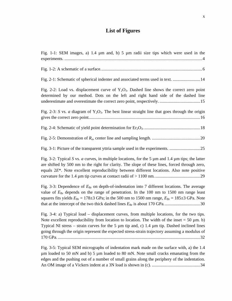
List of Figures

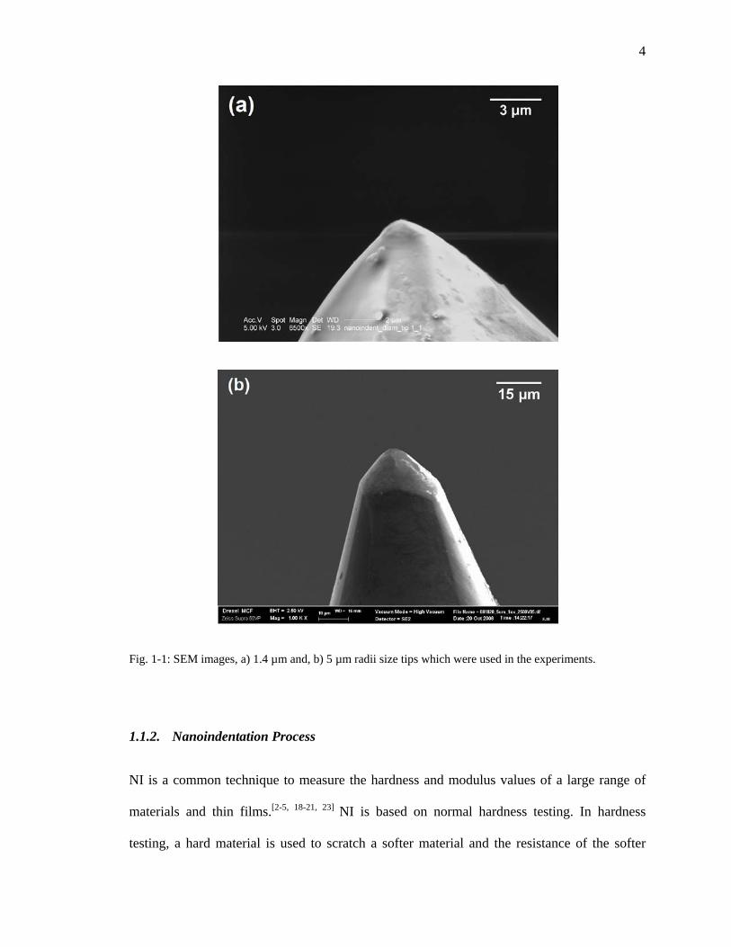
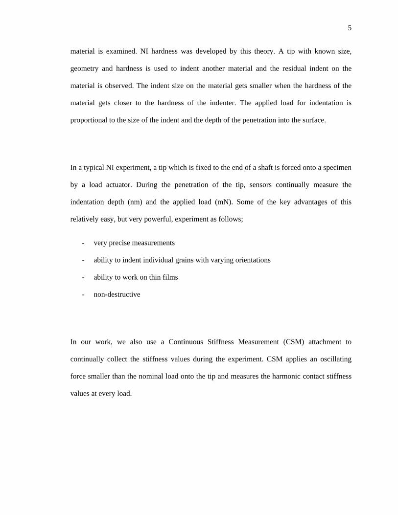
Fig. 1-1: SEM images, a) 1.4 µm and, b) 5 µm radii size tips which were used in the experiments. .............................................................................................................................. 4

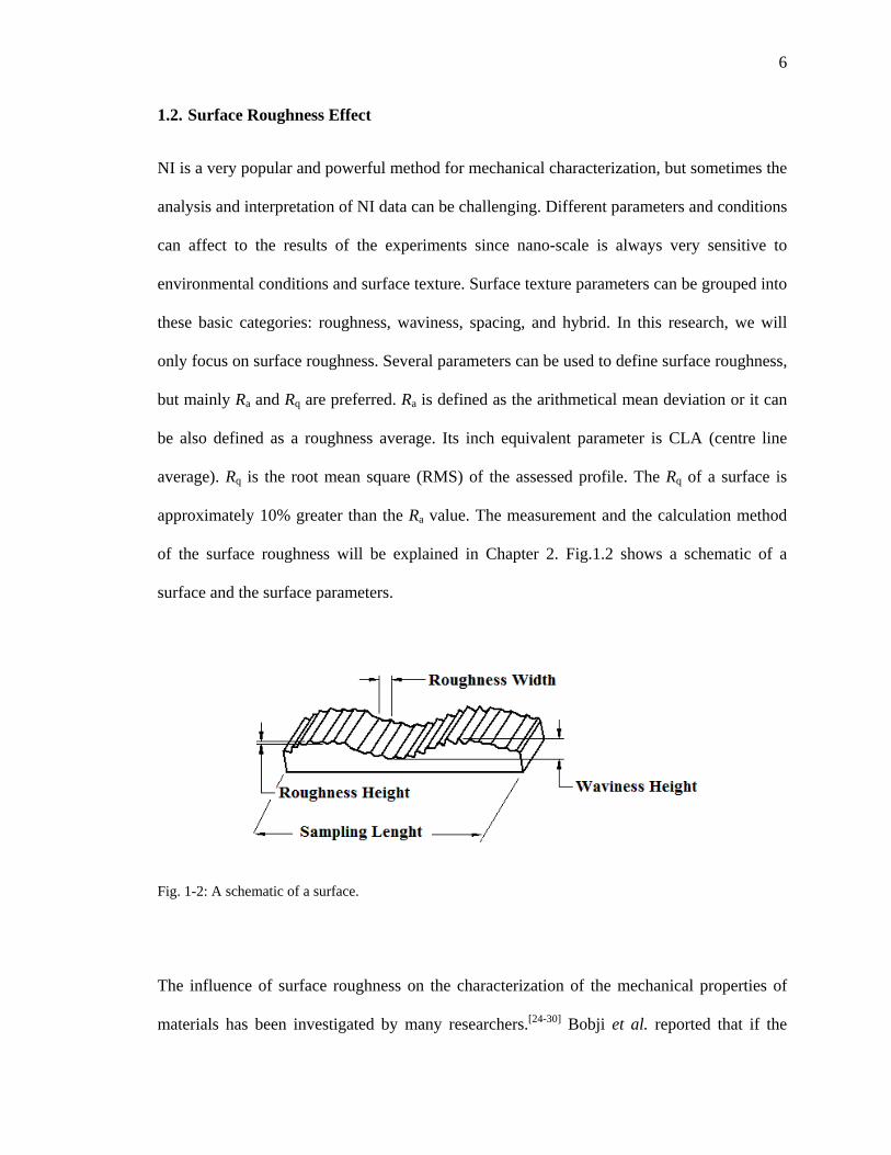
Fig. 1-2: A schematic of a surface. ............................................................................................ 6

Fig. 2-1: Schematic of spherical indenter and associated terms used in text. ......................... 14

Fig. 2-2: Load vs. displacement curve of Y2O3. Dashed line shows the correct zero point determined by our method. Dots on the left and right hand side of the dashed line underestimate and overestimate the correct zero point, respectively. ..................................... 15

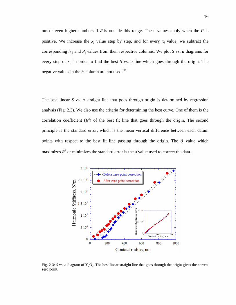
Fig. 2-3: S vs. a diagram of Y2O3. The best linear straight line that goes through the origin gives the correct zero point. ..................................................................................................... 16

Fig. 2-4: Schematic of yield point determination for Er2O3. ................................................... 18

Fig. 2-5: Demonstration of Ra, center line and sampling length. ............................................ 20

Fig. 3-1: Picture of the transparent yttria sample used in the experiments. ............................ 25

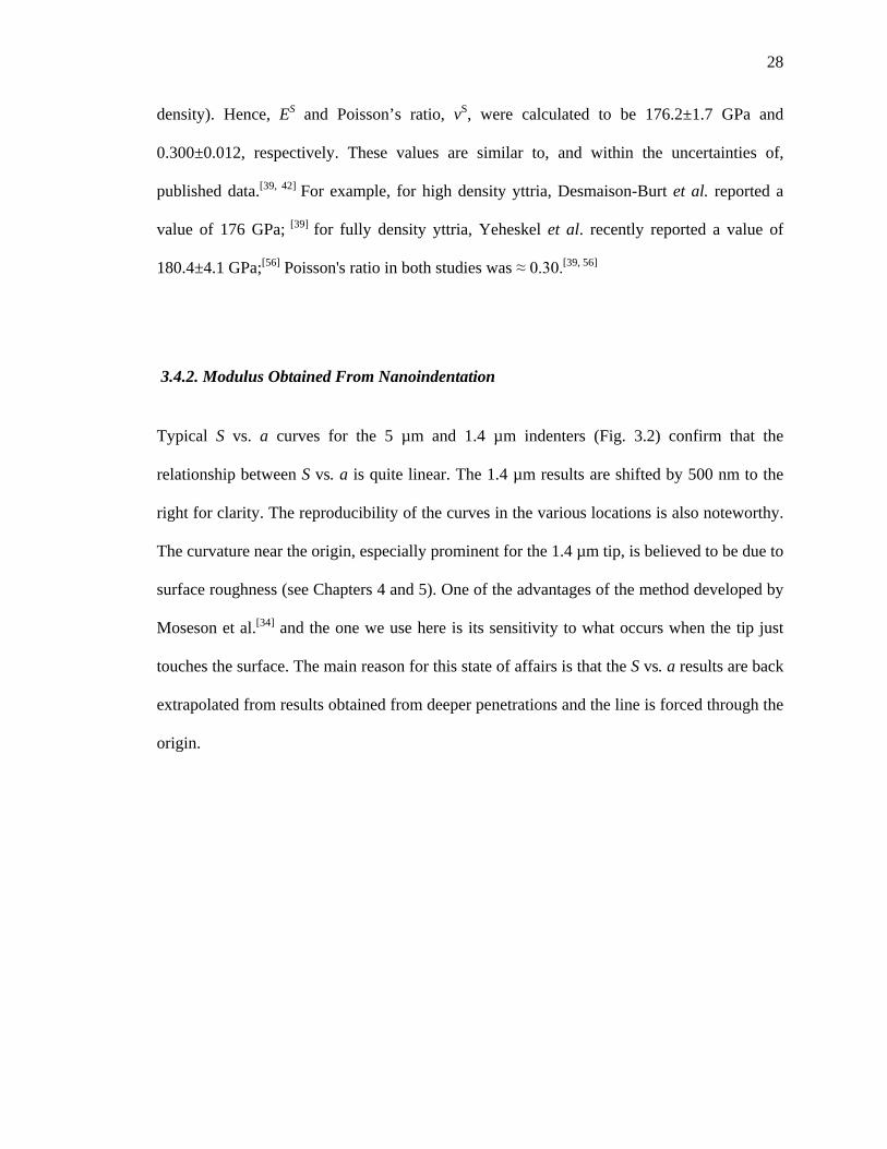
Fig. 3-2: Typical S vs. a curves, in multiple locations, for the 5 µm and 1.4 µm tips; the latter are shifted by 500 nm to the right for clarity. The slope of these lines, forced through zero, equals 2E*. Note excellent reproducibility between different locations. Also note positive curvature for the 1.4 µm tip curves at contact radii of > 1100 nm. ......................................... 29

Fig. 3-3: Dependence of EBr on depth-of-indentation into 7 different locations. The average value of EBr depends on the range of penetration. In the 100 nm to 1500 nm range least squares fits yields EBr = 178±3 GPa; in the 500 nm to 1500 nm range, EBr = 185±3 GPa. Note that at the intercept of the two thick dashed lines EBr is about 170 GPa. ................................ 30

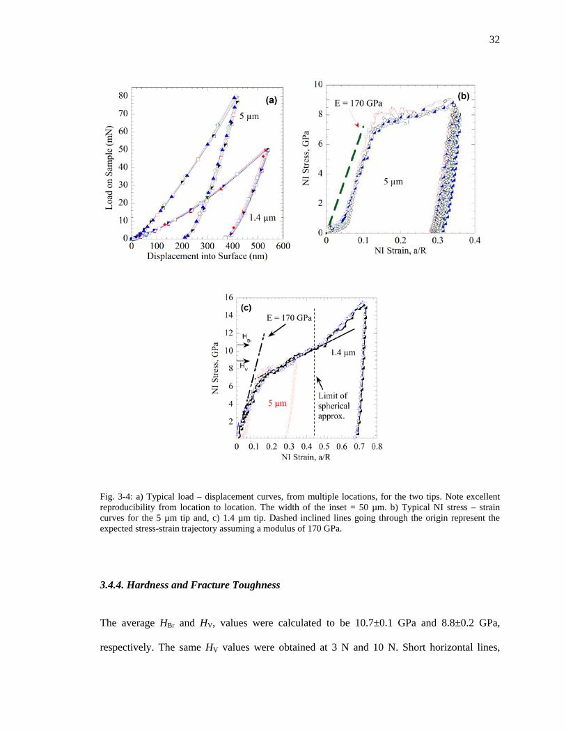
Fig. 3-4: a) Typical load – displacement curves, from multiple locations, for the two tips. Note excellent reproducibility from location to location. The width of the inset = 50 µm. b) Typical NI stress – strain curves for the 5 µm tip and, c) 1.4 µm tip. Dashed inclined lines going through the origin represent the expected stress-strain trajectory assuming a modulus of 170 GPa. .................................................................................................................................. 32

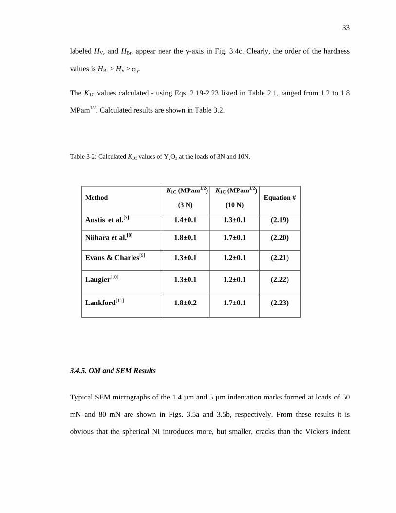
Fig. 3-5: Typical SEM micrographs of indentation mark made on the surface with, a) the 1.4 µm loaded to 50 mN and b) 5 µm loaded to 80 mN. Note small cracks emanating from the edges and the pushing out of a number of small grains along the periphery of the indentation. An OM image of a Vickers indent at a 3N load is shown in (c). ............................................ 34

xi

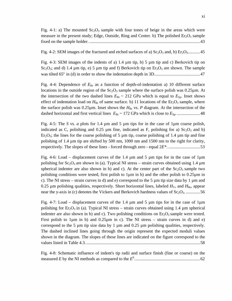
Fig. 4-1: a) The mounted Sc2O3 sample with four tones of beige in the areas which were measure in the present study; Edge, Outside, Ring and Center. b) The polished Er2O3 sample fixed on the sample holder. ..................................................................................................... 43

Fig. 4-2: SEM images of the fractured and etched surfaces of a) Sc2O3 and, b) Er2O3. .......... 45

Fig. 4-3: SEM images of the indents of a) 1.4 µm tip, b) 5 µm tip and c) Berkovich tip on Sc2O3; and d) 1.4 µm tip, e) 5 µm tip and f) Berkovich tip on Er2O3 are shown. The sample was tilted 65° in (d) in order to show the indentation depth in 3D. ......................................... 47

Fig. 4-4: Dependence of EBr as a function of depth-of-indentation a) 10 different surface locations in the outside region of the Sc2O3 sample where the surface polish was 0.25µm. At the intersection of the two dashed lines EBr ~ 212 GPa which is equal to ESp. Inset shows effect of indentation load on HBr of same surface. b) 11 locations of the Er2O3 sample, where the surface polish was 0.25µm. Inset shows the HBr vs. P diagram. At the intersection of the dashed horizontal and first vertical lines EBr ~ 172 GPa which is close to ESp. ..................... 48

Fig. 4-5: The S vs. a plots for 1.4 µm and 5 µm tips for in the case of 1µm coarse polish, indicated as C, polishing and 0.25 µm fine, indicated as F, polishing for a) Sc2O3 and b) Er2O3; the lines for the coarse polishing of 5 µm tip, coarse polishing of 1.4 µm tip and fine polishing of 1.4 µm tip are shifted by 500 nm, 1000 nm and 1500 nm to the right for clarity, respectively. The slopes of these lines - forced through zero - equal 2E*. ............................. 53

Fig. 4-6: Load – displacement curves of the 1.4 µm and 5 µm tips for in the case of 1µm polishing for Sc2O3 are shown in (a). Typical NI stress – strain curves obtained using 1.4 µm spherical indenter are also shown in b) and c). At the center part of the Sc2O3 sample two polishing conditions were tested, first polish to 1µm in b) and the other polish to 0.25µm in c). The NI stress – strain curves in d) and e) correspond to the 5 µm tip size data by 1 µm and 0.25 µm polishing qualities, respectively. Short horizontal lines, labeled HV, and HBr, appear near the y-axis in (c) denotes the Vickers and Berkovich hardness values of Sc2O3. ............. 56

Fig. 4-7: Load – displacement curves of the 1.4 µm and 5 µm tips for in the case of 1µm polishing for Er2O3 in (a). Typical NI stress – strain curves obtained using 1.4 µm spherical indenter are also shown in b) and c). Two polishing conditions on Er2O3 sample were tested. First polish to 1µm in b) and 0.25µm in c). The NI stress – strain curves in d) and e) correspond to the 5 µm tip size data by 1 µm and 0.25 µm polishing qualities, respectively. The dashed inclined lines going through the origin represent the expected moduli values shown in the diagram. The slopes of these lines are indicated on the figure correspond to the values listed in Table 4.3. ........................................................................................................ 58

Fig. 4-8: Schematic influence of indent's tip radii and surface finish (fine or coarse) on the measured E by the NI methods as compared to the ES. ........................................................... 62

xii

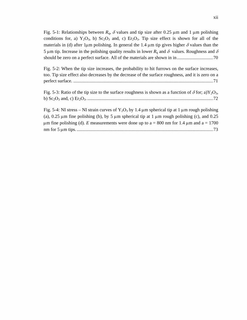
Fig. 5-1: Relationships between Rq, δ values and tip size after 0.25 µm and 1 µm polishing conditions for, a) Y2O3, b) Sc2O3 and, c) Er2O3. Tip size effect is shown for all of the materials in (d) after 1µm polishing. In general the 1.4 µm tip gives higher δ values than the 5 µm tip. Increase in the polishing quality results in lower Rq and δ values. Roughness and δ should be zero on a perfect surface. All of the materials are shown in in ............................... 70

Fig. 5-2: When the tip size increases, the probability to hit furrows on the surface increases, too. Tip size effect also decreases by the decrease of the surface roughness, and it is zero on a perfect surface. ........................................................................................................................ 71

Fig. 5-3: Ratio of the tip size to the surface roughness is shown as a function of δ for; a)Y2O3, b) Sc2O3 and, c) Er2O3. ............................................................................................................ 72

Fig. 5-4: NI stress – NI strain curves of Y2O3 by 1.4 µm spherical tip at 1 µm rough polishing (a), 0.25 µm fine polishing (b), by 5 µm spherical tip at 1 µm rough polishing (c), and 0.25 µm fine polishing (d). E measurements were done up to a = 800 nm for 1.4 µm and a = 1700 nm for 5 µm tips. ..................................................................................................................... 73

xiii

ABSTRACT Mechanical Properties of Polycrystalline Ceramics by Nanoindentation Methods: Effect of

Surface Roughness and Tip Size Ismail C. Albayrak

Advisor: Prof. Michel W. Barsoum Co-advisor: Prof. Ori Yeheskel

Nanoindentation, NI, – mainly with sharp tips - is a powerful method for the

mechanical characterization of solids. When the indenters are sharp, however, valuable

information concerning the all-important elastic-to-plastic transition is lost. Spherical tips, on

the other hand, do not suffer from this problem. In this work, we used 1.4 µm and 5 µm radii,

R, spherical diamond indenters to measure the moduli, E, and generate NI stress–strain

curves of the polycrystalline sesquioxides Y2O3, Sc2O3 and Er2O3. The moduli - measured

from harmonic contact stiffness (S) vs. contact radius (a) curves – were found to be weak

functions of R and slightly lower than the moduli measured by ultrasound on the same

samples used for the NI measurements.

This work also shows that surface finish – that was varied and quantified by

measuring the surface roughness - is an important factor in determining both the values of E,

and the shapes of the NI stress-strain curves, especially near the origin. In all cases, fine

polishing yielded results that were closer to the true values as measured by ultrasound. The

values of E measured by the Berkovich indenter were less sensitive to surface roughness.

When the hardness values measured using the Berkovich and Vickers indenters were

compared with the yield points obtained from the NI stress-strain curves the order was:

Berkovich, Vickers followed by the yield point. This conclusion is in agreement with

previous work on brittle single crystals.

xiv

Based on this work, we conclude that S vs. a plots are a powerful method to measure

the Young’s moduli of polycrystalline ceramics and other hard solids. The fact that one also

obtains NI stress–strain curves is a distinct advantage over the more commonly used load–

displacement curves. The influence of surface roughness, tip size and type are important

consideration when characterization of mechanical characterization at the nano-scale.

xv

1

Chapter 1 : INTRODUCTION

1.1. Nanoindentation Background

Nanoindentation has been widely used to determine the mechanical properties of many kinds

of materials for years. The easy application process of nanoindentation experiments makes it

very attractive to researchers. Several indentation methods and calculation theories have been

created for the characterization of the mechanical properties of the materials for a century.[1-5]

Until the past two decades, these methods mostly focused on finding the hardness values of

solids.[1] For these purposes, different size and different shape indenters were created. The

most common indentation method is the Vickers microhardness indentation which is also

known as the classical indentation method. The Vickers microhardness tip is a four faced

pyramidal tip where the lengths of the diagonals are in the scale of µm. After the indentation

process, a diamond shaped indent is created, and usually cracks are observed at the corners of

the diagonals in brittle solids. This indentation method has been frequently used for

measuring the hardness of solids and also the calculation of the fracture toughness by

measuring the size of the cracks emanating from corners of the indents.[1, 6-11] The

disadvantage of the Vickers indentation is that it does not provide any information other than

the hardness and sometimes an approximate value of fracture toughness.

Over the past two decades, nanoindentation, NI, in which both the load and displacement are

continually measured, has become quite popular. The advantage of the NI techniques is that

in addition to measuring the hardness of a solid, they can also measure the moduli. New

2

developments of test systems opened a door to new sizes of tips for the mechanical

characterization by NI methods. Berkovich indenters are one of the tip types which are

commonly used by researchers in the mechanical characterization area.[2, 3] They have a

three-faced pyramidal shape and create triangle-shaped indents on the material’s surface.

Berkovich tips have the same area-to-depth function as Vickers microhardness indenters, but

with a smaller tip size. They are sharper than Vickers tips. Cube corner tips are sharper than

even Berkovich tips, they have three faces, but they have the shape of the corner of a cube.

Vickers microhardness, Berkovich and cube corner indenters are sharp; therefore, they do not

allow for the collecting enough data during the initial elastic region of the indentation.

Whenever the sharpness increases, the stress and strain produced around the indents

increases. Because of the sharp indenter shape, penetration becomes very rough, and the

material deforms plastically by the penetration of the tip quickly even when the initial load is

quite low. In other words, any all information on the important elastic-to-plastic transition is

lost. As this work shows, this is not true of spherical indenters.

1.1.1. Spherical Indentation

The history of spherical indenters starts with Brinell[12]. In the last two decades, because of

the increase of the importance of nano-scale measurements, spherical NI became the

preferred method of material characterization by many researchers, and the calculations

methods for the characterization of mechanical properties were developed and improved.[4, 13,

14] The method developed by Field and Swain[4] was adopted by most of the researchers of the

material characterization area.

3

As noted above, spherical tips allowed researchers to collect more data around the initial

elastic part of the indentation test before the material started deforming plastically. Spherical

indenters allow us to use the beginning part of the loading data because of the ability of soft

penetration to the surface and the possibility of obtaining more data points in the elastic

regime.

Because of the lack of enough data during the penetration of the tip into the surface, load on

the sample vs. displacement into surface diagrams were plotted for material

characterization.[2, 4, 5, 15, 16] However these plots cannot give so much information about the

mechanical properties of the material. Another positive feature of the spherical indentation is

that the method enables the ability of plotting more informative indentation stress vs.

indentation strain diagrams since there is changing in the strain by the change of the stress.[16]

By this way, yield strength, strain hardening and maximum stresses can be characterized. The

idea to use indentation strain and stress in metals was put forward 6 decades ago;[1]

Since then micro-indentation[4, 17] and NI[2, 3, 5, 18-22] techniques were devised to study the

elastic moduli and mechanical behavior of materials. The method of how to obtain

indentation stress vs. strain curves will be explained in Chapter 2. This thesis mostly will be

focused on spherical indentation and their corresponding stress vs. strain curves. We used

two different sizes of spherical tips, 1.4 µm and 5µm. SEM pictures of the tips shown in Figs

1.1a and 1.1b. Berkovich and Vickers microhardness indentations were used for hardness and

elastic moduli comparisons, and also the calculations of fracture toughness.

4

Fig. 1-1: SEM images, a) 1.4 µm and, b) 5 µm radii size tips which were used in the experiments.

1.1.2. Nanoindentation Process

NI is a common technique to measure the hardness and modulus values of a large range of

materials and thin films.[2-5, 18-21, 23] NI is based on normal hardness testing. In hardness

testing, a hard material is used to scratch a softer material and the resistance of the softer

5

material is examined. NI hardness was developed by this theory. A tip with known size,

geometry and hardness is used to indent another material and the residual indent on the

material is observed. The indent size on the material gets smaller when the hardness of the

material gets closer to the hardness of the indenter. The applied load for indentation is

proportional to the size of the indent and the depth of the penetration into the surface.

In a typical NI experiment, a tip which is fixed to the end of a shaft is forced onto a specimen

by a load actuator. During the penetration of the tip, sensors continually measure the

indentation depth (nm) and the applied load (mN). Some of the key advantages of this

relatively easy, but very powerful, experiment as follows;

- very precise measurements

- ability to indent individual grains with varying orientations

- ability to work on thin films

- non-destructive

In our work, we also use a Continuous Stiffness Measurement (CSM) attachment to

continually collect the stiffness values during the experiment. CSM applies an oscillating

force smaller than the nominal load onto the tip and measures the harmonic contact stiffness

values at every load.

6

1.2. Surface Roughness Effect

NI is a very popular and powerful method for mechanical characterization, but sometimes the

analysis and interpretation of NI data can be challenging. Different parameters and conditions

can affect to the results of the experiments since nano-scale is always very sensitive to

environmental conditions and surface texture. Surface texture parameters can be grouped into

these basic categories: roughness, waviness, spacing, and hybrid. In this research, we will

only focus on surface roughness. Several parameters can be used to define surface roughness,

but mainly Ra and Rq are preferred. Ra is defined as the arithmetical mean deviation or it can

be also defined as a roughness average. Its inch equivalent parameter is CLA (centre line

average). Rq is the root mean square (RMS) of the assessed profile. The Rq of a surface is

approximately 10% greater than the Ra value. The measurement and the calculation method

of the surface roughness will be explained in Chapter 2. Fig.1.2 shows a schematic of a

surface and the surface parameters.

Fig. 1-2: A schematic of a surface.

The influence of surface roughness on the characterization of the mechanical properties of

materials has been investigated by many researchers.[24-30] Bobji et al. reported that if the

7

surface was rough, there was always a scatter in hardness which decreased with increasing

penetration depth.[24] Jiang et al. also observed that surface roughness significantly influenced

both the hardness and Young’s moduli of thin films.[27] Kim et al. observed a decrease in

hardness and Young’s moduli values when the surface was rough.[26] Walter et al.[30] showed

that surface roughness resulted in an underestimation of the determined Young’s moduli. The

effect of the surface roughness on the NI stress – strain and S vs. a curves will be discussed in

Ch. 4. The effect of polishing quality on the effective zero point value is discussed in Ch. 5.

1.3. Structure of the Thesis

In the introduction, we briefly reviewed the history of indentation. We mentioned the tips

which have been used for decades for the mechanical characterization of materials.

Commonly used, sharp tips lead to plastic deformation quickly after penetration. Therefore

we introduced the less sharp spherical tips which are the main tips we used herein. We

mentioned the stress-strain curves produced by using spherical NI tips and also the working

process of the nanoindenters. Finally, we briefly introduced surface roughness and its effects

on the material characterization.

In the Ch. 2, we outline the theory of how to plot spherical NI stress vs. strain diagrams in the

elastic and elasto-plastic regimes. We will introduce a method to plot harmonic contact

stiffness vs. contact radius diagrams, which are the main diagrams that we use to calculate

the reduced Young’s moduli values. Equations for the calculations of hardness and fracture

toughness are also listed in this chapter. We will explain the measurement and calculation

8

method of surface roughness. At the end of the chapter, we will describe the experimental

methods that were used in this study.

Chapter 3 will focus on the mechanical properties of polycrystalline Y2O3 and the effect of tip

size and type on the results. In the fourth chapter, we describe the mechanical properties of

polycrystalline materials Sc2O3 and Er2O3 as determined from NI. The effects of tip size,

surface roughness and polishing quality on the mechanical characterization of these materials

will be outlined.

Chapter 5 will discuss the relations between surface roughness, polishing quality, tip size and

the effective zero point correction. This chapter will verify the discussion in the Ch. 4. The

thesis will be summarized and concluded in the Ch. 6.

9

Chapter 2 : THEORY AND EXPERIMENTAL PROCEDURES

2.1. Theory

2.1.1 Spherical Nanoindentation Stress-Strain Analysis

In a typical NI experiment, the load (P) and total displacement into the surface (htot) values

are collected. Harmonic contact stiffness (S) values can also be obtained if the NI is equipped

with a continuous stiffness measurement (CSM) option.[2, 4, 19] S is continually measured by

superimposing a harmonic force, on the nominally increasing load applied during NI.[19] The

model described here is generally based on the developments on the method first suggested

by Herbert et al.[13]

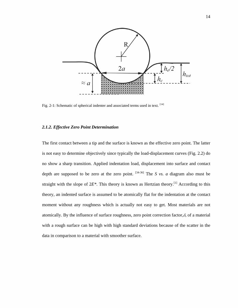
Fig. 2.1 depicts the requisite parameters – elastic distance into the surface (he), contact depth

(hc), total displacement into surface (htot), contact radius (a), and the spherical tip radius (R) -

needed for the calculation of the NI stress-strain curves.[14]

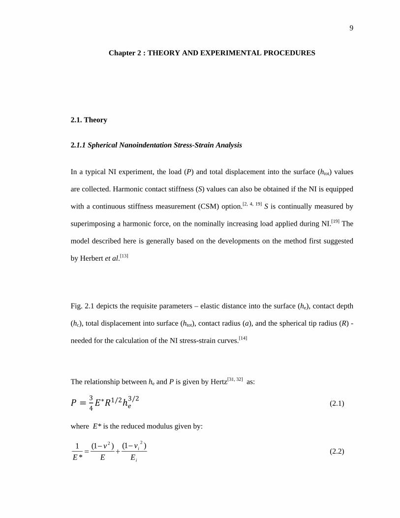
The relationship between he and P is given by Hertz[31, 32] as:

𝑃𝑃 = 34𝐸𝐸∗𝑅𝑅1/2ℎ𝑒𝑒

3/2 (2.1)

where E* is the reduced modulus given by:

i

i

Ev

Ev

E)1()1(

*1 22 −

+−

= (2.2)

10

νi and Ei are the Poisson’s ratio and Young’s modulus of the indenter, respectively, and ν and

E are the Poisson’s ratio and spherical Young’s modulus of the material, respectively. We

used vi =0.07 and Ei = 1141 GPa for the diamond tip.[19]

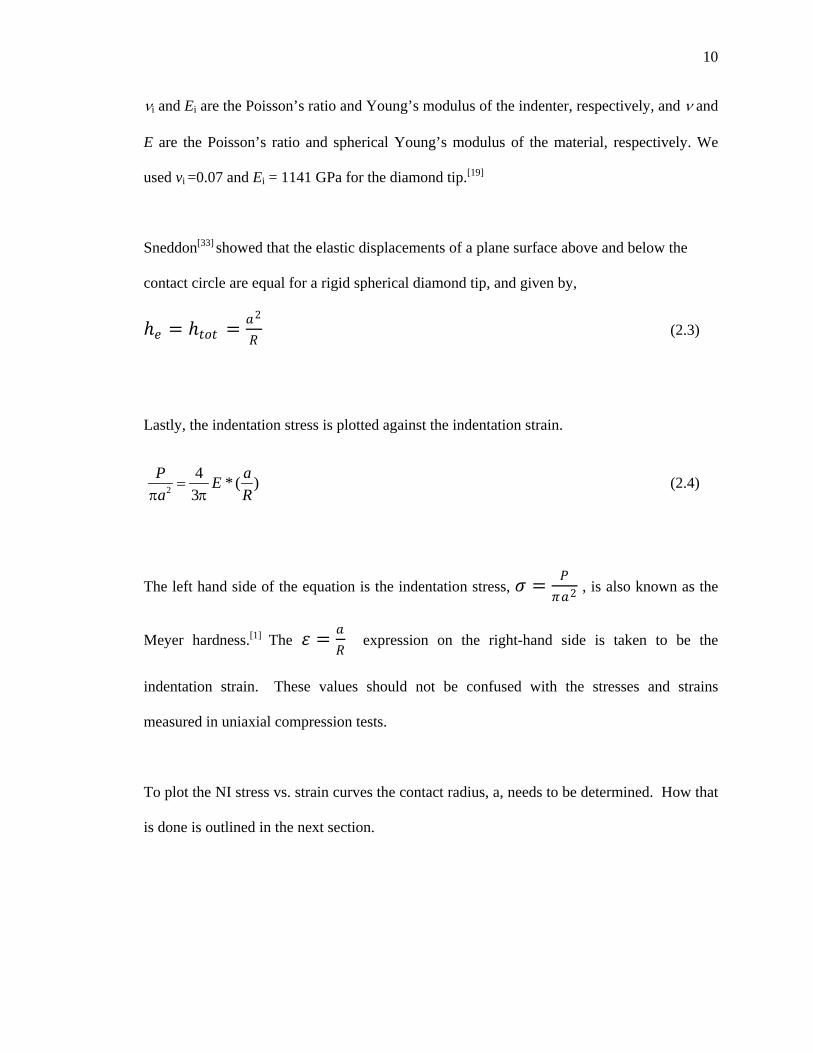
Sneddon[33] showed that the elastic displacements of a plane surface above and below the

contact circle are equal for a rigid spherical diamond tip, and given by,

ℎ𝑒𝑒 = ℎ𝑡𝑡𝑡𝑡𝑡𝑡 = 𝑎𝑎2

𝑅𝑅 (2.3)

Lastly, the indentation stress is plotted against the indentation strain.

(2.4)

The left hand side of the equation is the indentation stress, 𝜎𝜎 = 𝑃𝑃𝜋𝜋𝑎𝑎2 , is also known as the

Meyer hardness.[1] The 𝜀𝜀 = 𝑎𝑎

𝑅𝑅 expression on the right-hand side is taken to be the

indentation strain. These values should not be confused with the stresses and strains

measured in uniaxial compression tests.

To plot the NI stress vs. strain curves the contact radius, a, needs to be determined. How that

is done is outlined in the next section.

Pπa2 =

43π

E * ( aR

)

11

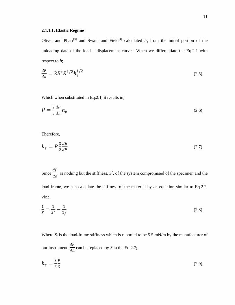
2.1.1.1. Elastic Regime

Oliver and Pharr[3] and Swain and Field[4] calculated he from the initial portion of the

unloading data of the load – displacement curves. When we differentiate the Eq.2.1 with

respect to h;

𝑑𝑑𝑃𝑃𝑑𝑑ℎ

= 2𝐸𝐸∗𝑅𝑅1/2ℎ𝑒𝑒1/2

(2.5)

Which when substituted in Eq.2.1, it results in;

𝑃𝑃 = 23𝑑𝑑𝑃𝑃𝑑𝑑ℎℎ𝑒𝑒 (2.6)

Therefore,

ℎ𝑒𝑒 = 𝑃𝑃 32𝑑𝑑ℎ𝑑𝑑𝑃𝑃

(2.7)

Since 𝑑𝑑𝑃𝑃𝑑𝑑ℎ

is nothing but the stiffness, S*, of the system compromised of the specimen and the

load frame, we can calculate the stiffness of the material by an equation similar to Eq.2.2,

viz.;

1𝑆𝑆

= 1𝑆𝑆∗− 1

𝑆𝑆𝑓𝑓 (2.8)

Where Sf is the load-frame stiffness which is reported to be 5.5 mN/m by the manufacturer of

our instrument. 𝑑𝑑𝑃𝑃𝑑𝑑ℎ

can be replaced by S in the Eq.2.7;

ℎ𝑒𝑒 = 32𝑃𝑃𝑆𝑆

(2.9)

12

Since we obtained the equation of he, we can easily calculate a by the knowledge of P and S,

and using Eq.2.3.

2.1.1.2. Elasto-plastic Regime

Both Oliver and Pharr[3] and Swain and Field[4] assumed that the contact depth, hc, is the

distance from the contact circle of the tip to the maximum penetration depth as shown in

Fig.2.1, one can calculate hc by;

ℎ𝑐𝑐 ≈ ℎ𝑡𝑡𝑡𝑡𝑡𝑡 −ℎ𝑒𝑒2

(2.10)

When we combine Eq.2.9 and Eq.2.10, we obtain,

ℎ𝑐𝑐 = ℎ𝑡𝑡𝑡𝑡𝑡𝑡 − (34𝑃𝑃𝑆𝑆

) (2.11)

Eq.2.11 can be modified for the effective zero point correction by addition of δ as;

ℎ𝑐𝑐 = ℎ𝑡𝑡𝑡𝑡𝑡𝑡 − (34𝑃𝑃𝑆𝑆

) ± 𝛿𝛿 (2.12)

δ is in the scale of a few nanometers and it is adjustable depending on the surface conditions.

Once hc is calculated, a is defined assuming:

𝑎𝑎 = �2𝑅𝑅ℎ𝑐𝑐 − ℎ𝑐𝑐2 ≈ �2𝑅𝑅ℎ𝑐𝑐 (2.13)

13

The right hand side of the equation only applies when ℎ𝑐𝑐 ≪ 𝑎𝑎 and the tip is perfectly

spherical. We should note that in the purely elastic regime, ℎ𝑐𝑐 = ℎ𝑡𝑡𝑡𝑡𝑡𝑡2

= ℎ𝑒𝑒2

so Eq.2.3 and

Eq.2.10 become identical. Note that in the plastic regime, most of the time ℎ𝑡𝑡𝑡𝑡𝑡𝑡 ≫ℎ𝑒𝑒2

, so

ℎ𝑐𝑐 ≈ ℎ𝑡𝑡𝑡𝑡𝑡𝑡 (Eq.2.10).

Given that for an isotropic elastic solid, indented with a spherical indenter: [3, 13, 31]

𝑆𝑆 = 2𝐸𝐸∗𝑎𝑎 (2.14)

it follows that the slope of S vs. a plots should also yield E*, from which the Young's

modulus obtained using a spherical indenter, ESp, can be directly calculated from Eq. 2.2.

Theoretically, it is important to note that the S vs. a curve must be linear and go through the

origin. The latter is critical herein because, as discussed below, it renders the determination

of δ accurate and objective.

14

Fig. 2-1: Schematic of spherical indenter and associated terms used in text. [14]

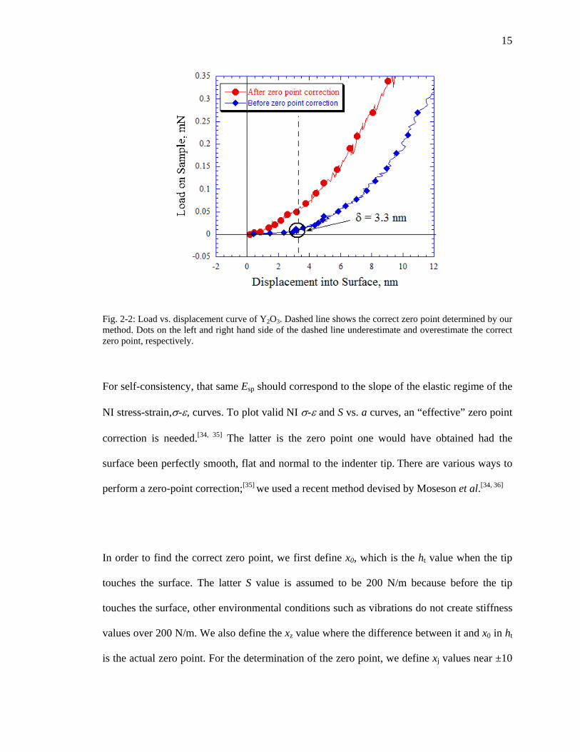
2.1.2. Effective Zero Point Determination

The first contact between a tip and the surface is known as the effective zero point. The latter

is not easy to determine objectively since typically the load-displacement curves (Fig. 2.2) do

no show a sharp transition. Applied indentation load, displacement into surface and contact

depth are supposed to be zero at the zero point. [34-36] The S vs. a diagram also must be

straight with the slope of 2E*. This theory is known as Hertzian theory.[1] According to this

theory, an indented surface is assumed to be atomically flat for the indentation at the contact

moment without any roughness which is actually not easy to get. Most materials are not

atomically. By the influence of surface roughness, zero point correction factor,δ, of a material

with a rough surface can be high with high standard deviations because of the scatter in the

data in comparison to a material with smoother surface.

15

Fig. 2-2: Load vs. displacement curve of Y2O3. Dashed line shows the correct zero point determined by our method. Dots on the left and right hand side of the dashed line underestimate and overestimate the correct zero point, respectively.

For self-consistency, that same Esp should correspond to the slope of the elastic regime of the

NI stress-strain,σ-ε, curves. To plot valid NI σ-ε and S vs. a curves, an “effective” zero point

correction is needed.[34, 35] The latter is the zero point one would have obtained had the

surface been perfectly smooth, flat and normal to the indenter tip. There are various ways to

perform a zero-point correction;[35] we used a recent method devised by Moseson et al.[34, 36]

In order to find the correct zero point, we first define x0, which is the ht value when the tip

touches the surface. The latter S value is assumed to be 200 N/m because before the tip

touches the surface, other environmental conditions such as vibrations do not create stiffness

values over 200 N/m. We also define the xz value where the difference between it and x0 in ht

is the actual zero point. For the determination of the zero point, we define xj values near ±10

16

nm or even higher numbers if δ is outside this range. These values apply when the P is

positive. We increase the xj value step by step, and for every xj value, we subtract the

corresponding ht,j and Pj values from their respective columns. We plot S vs. a diagrams for

every step of xj, in order to find the best S vs. a line which goes through the origin. The

negative values in the ht column are not used.[36]

The best linear S vs. a straight line that goes through origin is determined by regression

analysis (Fig. 2.3). We also use the criteria for determining the best curve. One of them is the

correlation coefficient (R2) of the best fit line that goes through the origin. The second

principle is the standard error, which is the mean vertical difference between each datum

points with respect to the best fit line passing through the origin. The δj value which

maximizes R2 or minimizes the standard error is the δ value used to correct the data.

Fig. 2-3: S vs. a diagram of Y2O3. The best linear straight line that goes through the origin gives the correct zero point.

17

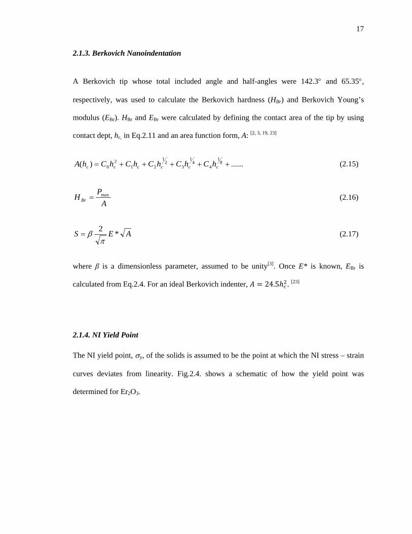
2.1.3. Berkovich Nanoindentation

A Berkovich tip whose total included angle and half-angles were 142.3° and 65.35°,

respectively, was used to calculate the Berkovich hardness (HBr) and Berkovich Young’s

modulus (EBr). HBr and EBr were calculated by defining the contact area of the tip by using

contact dept, hc, in Eq.2.11 and an area function form, A: [2, 3, 19, 23]

......)( 81

44

1

32

1

212

0 +++++= cccccc hChChChChChA (2.15)

AP

H Brmax= (2.16)

AES *2π

β= (2.17)

where β is a dimensionless parameter, assumed to be unity[3]. Once E* is known, EBr is

calculated from Eq.2.4. For an ideal Berkovich indenter, 𝐴𝐴 = 24.5ℎ𝑐𝑐2. [23]

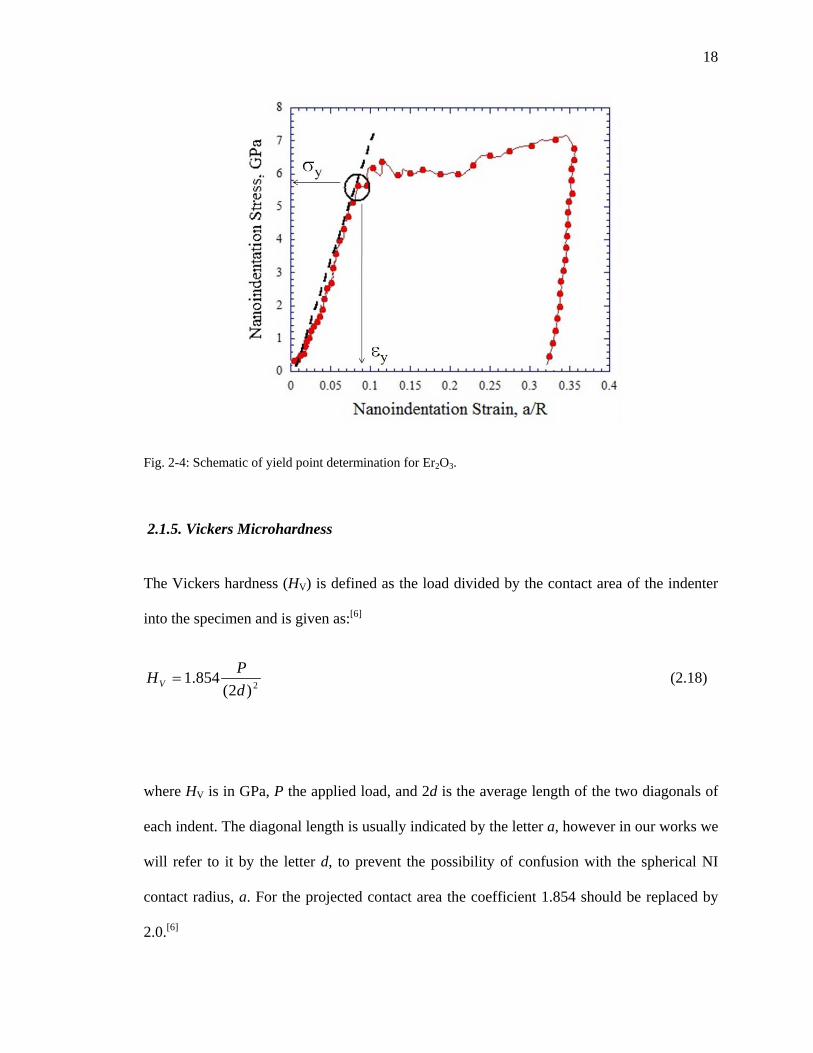
2.1.4. NI Yield Point

The NI yield point, σy, of the solids is assumed to be the point at which the NI stress – strain

curves deviates from linearity. Fig.2.4. shows a schematic of how the yield point was

determined for Er2O3.

18

Fig. 2-4: Schematic of yield point determination for Er2O3.

2.1.5. Vickers Microhardness

The Vickers hardness (HV) is defined as the load divided by the contact area of the indenter

into the specimen and is given as:[6]

2)2(854.1

dPHV = (2.18)

where HV is in GPa, P the applied load, and 2d is the average length of the two diagonals of

each indent. The diagonal length is usually indicated by the letter a, however in our works we

will refer to it by the letter d, to prevent the possibility of confusion with the spherical NI

contact radius, a. For the projected contact area the coefficient 1.854 should be replaced by

2.0.[6]

19

2.1.6. Fracture Toughness

In our work, the indentation fracture toughness (K1C) was evaluated from the Vickers

hardness indents [7-11, 37, 38] and is referred to as Vickers indentation fracture toughness. The

K1C values were calculated according to the equations listed in Table 2.1[39] We note that

measuring twice the crack size (2c) was somewhat problematic, since in some cases the

cracks were not fully developed after unloading.[40] To enhance and better observe the cracks,

the surface was polished for 60 s on a cloth with a 1 µm diamond paste with no cooling liquid

after the Vickers indentations in our experiments. This procedure has been shown to work

well on transparent yttria when the latter is observed with oblique illumination or polarized

light, since it highlights the crack shadows enabling 2c to be accurately measured.[40]

Table 2-1: Indentation equations used for the calculation of K1C,[39] where, PV is the load applied in the Vickers hardness test, φ is a constraint factor (φ ~ 3), E, is the Young's modulus, HV, the Vickers hardness, c, the radius of the critical crack and, d, is half the diagonal of the Vickers indent.

Method Mathematical Expression Equation #

Anstis et al.[7] )/()/(018.0 5.15.01 cPHEK VVC = (2.19)

Niihara et al.[8] 4.021231 )/()/)(/129.0( VVC HEdHdcK φφ −= (2.20)

Evans & Charles[9] 2321 16.0 −= cdHK VC (2.21)

Laugier[10] )/()/(010.0 23321 cPHEK VVC = (2.22)

Lankford[11] 56.14.0231 )/()/(/142.0 −= dcHEdHK VVC φφ (2.23)

20

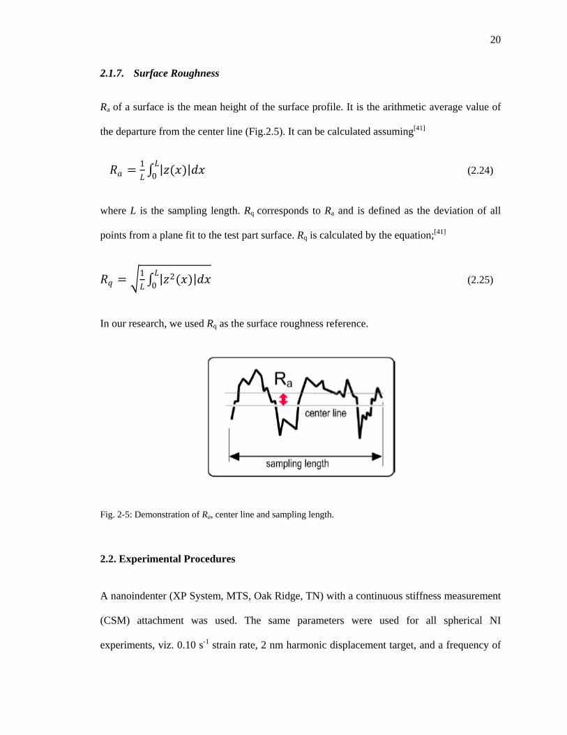
2.1.7. Surface Roughness

Ra of a surface is the mean height of the surface profile. It is the arithmetic average value of

the departure from the center line (Fig.2.5). It can be calculated assuming[41]

𝑅𝑅𝑎𝑎 = 1𝐿𝐿 ∫ |𝑧𝑧(𝑥𝑥)|𝑑𝑑𝑥𝑥𝐿𝐿

0 (2.24)

where L is the sampling length. Rq corresponds to Ra and is defined as the deviation of all

points from a plane fit to the test part surface. Rq is calculated by the equation;[41]

𝑅𝑅𝑞𝑞 = �1𝐿𝐿 ∫ |𝑧𝑧2(𝑥𝑥)|𝑑𝑑𝑥𝑥𝐿𝐿

0 (2.25)

In our research, we used Rq as the surface roughness reference.

Fig. 2-5: Demonstration of Ra, center line and sampling length.

2.2. Experimental Procedures

A nanoindenter (XP System, MTS, Oak Ridge, TN) with a continuous stiffness measurement

(CSM) attachment was used. The same parameters were used for all spherical NI

experiments, viz. 0.10 s-1 strain rate, 2 nm harmonic displacement target, and a frequency of

21

45 Hz. Two different diamond spherical tips with radii of 1.4 µm and 5 µm were used. Prior

to our measurements, the indenters were calibrated on a standard fused silica.

The tests were carried out at different load levels depending on the hardness of the materials.

Whenever a surface was detected by the NI, the tip was loaded at a fixed loading rate of

(dP/dt)/P = 0.1 s-1.[3] Using this loading rate, we were able to collect many data points during

the initial loading section when the tip is penetrating the surface. Using a fixed (dP/dt)/P also

gives us the possibility of producing a constant strain rate value, (dh/dt)/h. In this way, the

hardness is no longer a function of depth if the former is a function of the latter. The NI was

also calibrated with fused silica for the Berkovich tip. We assumed the elastic modulus of

fused silica to be 72 GPa. We bought two pieces and measured their modulus values by our

NI. We obtained 73.4 ± 0.6 GPa, and then changed the area function to a value that we

obtained the correct Young’s moduli.

A Vickers microhardness tester (M-400 Micro Hardness Tester, LECO Corp, St. Joseph, MI)

was also used to measure the Vickers microhardness for all of the materials we used in our

experiments. In all of the Vickers microhardness tests, we used the same surfaces of the

materials which were used for the NI experiments. Different loads were applied to the

materials, but dwell time was always 15 seconds.

The dynamic elastic modulus, ES, were calculated from the longitudinal and transverse sound

velocities, VL and VT, respectively, measured on all of the samples used for the indentation

22

tests. The velocities were measured using a pulse-echo method described elsewhere.[42] ES

calculations were made by Dr. Ori Yeheskel.

Berkovich indentation was applied to all of the materials in our experiments. HBr and EBr

values were calculated using the Oliver and Pharr[3] method, and the results were compared

with ESp, ES and HV values.

An Olympus PMG3 (Japan) metallographic microscope was used for optical microscopy

(OM), and a Zeiss Supra 50VP (Thornwood, NY) was used for Scanning Electron

Microscopy (SEM). These microscopes were both used for imaging the tips and indents for

the hardness and fracture toughness measurements.

Surface roughness measurements were done using an optical profilometer (Zygo NewView

600, Middlefield, CT).

23

Chapter 3 : MECHANICAL PROPERTIES OF YTTRIA and TIP SIZE EFFECT

3.1. Introduction

Yttria (Y2O3) is a cubic sesquioxide which is considered for various applications including

infrared (IR) missile domes,[43-46] as a host material for optical applications,[47-49] cutting

tools,[50] a structural material for high temperatures,[51] and as a coating or a crucible material

for molten reactive metals like Li,[50] Ti,[50] and U.[50, 52, 53]

Transparent yttria for IR applications is usually produced by a combination of pressureless

sintering at high temperature, T~2200 K,[43, 46] pressure-assisted sintering like hot pressing

(HP),[44, 49] and pressureless sintering at T~2150 K followed by high temperature hot isostatic

pressing (HIP), T~2050 K.[45] However, special pretreatments aimed at removing moisture

from the powder particles, followed by relatively low temperature HIP T~1600 K, yield

transparent Y2O3.[42]

Understanding the mechanical deformation behavior is required for all the applications

mentioned above. For high density Y2O3 the bending strengths were measured at room

temperature[39] and in compression at room and at high temperatures.[54] The strength

intensity factor in mode I, the fracture toughness, KIC, of high-purity, high-density yttria was

reported to be in the 1.2–1.8 MPa.m1/2 range depending on the equation used.[39, 55]

24

The technique developed to generate the room-temperature NI stress – strain curves from

spherical NI load – displacement curves was described in Ch. 2.[13, 14] The objective of this

chapter is to characterize the room-temperature mechanical properties of transparent yttria

using this newly developed technique and to compare the results with other more established

techniques, such as Vickers microhardness and Berkovich NI, and also to investigate the tip

size effect on the mechanical properties.

The present chapter focuses on the NI stress – strain curves of fully dense, transparent yttria.

E determined by the various methods also compared to the ES measured by ultrasound on the

same sample. The Vickers indentation fracture toughness, K1C, was also measured.

3.2. Experimental Details

3.2.1. Sample Processing

Yttria powder (Cerac, Milwaukee, WI), 99.9% pure, with an average particle size of ~ 0.5

µm, was cold isostatically pressed at 200 MPa. The compacts were heat-treated in air,

followed by 24 h heat treatment in vacuum (~ 3 Pa) to dry them. The pressed and treated

compact was then HIPed at 1350 °C under a pressure of 150 MPa for 1.5 h.[42] The sample

diameter and thickness were 18.7 mm, and 3.1 mm, respectively. The sample was polished

with 1 µm diamond paste before testing. The sample was transparent and the average grain

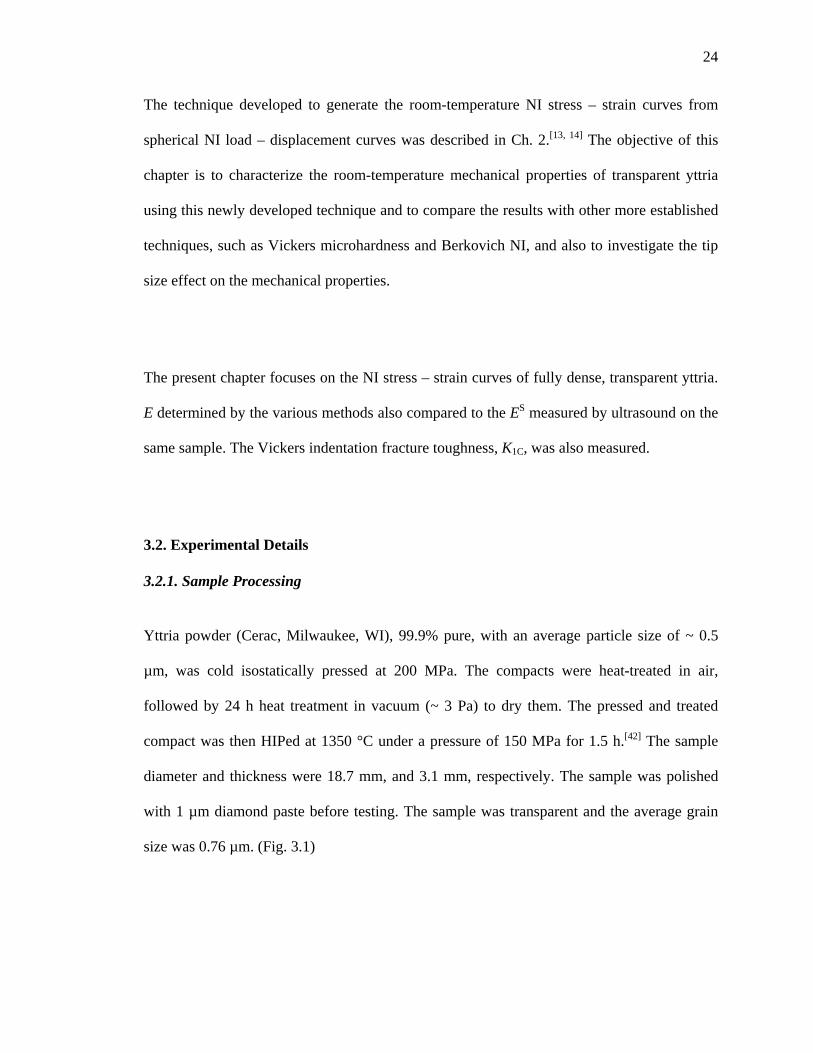
size was 0.76 µm. (Fig. 3.1)

25

Both an OM and a SEM were used to image the surfaces before and after the various

indentations.

Fig. 3-1: Picture of the transparent yttria sample used in the experiments.

3.3. Material Characterization

3.3.1. Dynamic Elastic Modulus

As noted above, ES was calculated from the longitudinal and transverse sound velocities, VL

and VT, respectively - measured on the same sample used for the indentation tests. The

velocities were measured using a pulse-echo method described elsewhere.[42] The sample’s

density (ρ) was measured using Archimedes' principle.[56] The uncertainty in the density

measurements is estimated to be ≈ ± 0.1%; that in VL ≈ ± 0.4%, and for VT ≈ ± 0.25%. The

resulting uncertainty in the ES is thus ≈ ±1 %, while that of the dynamic Poisson’s ratio (vS) is

± 5%.

26

3.3.2. Nanoindentation

A nanoindenter with a CSM attachment was used. The same parameters were used for all of

the spherical NIs, viz. 0.10 s-1 strain rate, 2 nm harmonic displacement target, and a

frequency of 45 Hz. Two different diamond spherical tips with radii of 1.4 µm and 5 µm

were used. The indenters were calibrated on fused silica before all of the experiments

applied.

In our work to date, we typically obtained the modulus of our surfaces – on mostly single

crystals [14, 57-61] from the slope of the S vs. a curves over their entire range. The results

obtained, when compared to the elastic constants, were deemed reasonable. In this work, we

first measured the ES and then calculated ESp from the various ranges of the S vs. a curves

and compared the two. The following ranges of S vs. a curves were used:

(M1) For the 1.4 µm tip, we used the S vs. a results up to values of a ≅ 800 nm; for the 5 µm

tip up to a ≅ 1700 nm. Above these values, the indenters are no longer spherical, in which

case Eq. 2.13 is no longer valid.

(M2) The S vs. a results, but only up to the yield stress. In this iterative approach, first the

stress-strain curves are determined and then the range of a in which the behavior is linear

elastic was determined and used.

27

Henceforth these methods are referred by their designations in parentheses. In all cases the S

vs. a data were corrected for the effective zero point.[34] The point at which the NI stress-

strain curves deviated from linearity was taken as the NI yield point, σy.

The maximum load used with the 5 µm tip was 80 mN; for the 1.4 µm tip it was 50 mN. Four

or five different locations were typically indented and ESp calculated using methods M1 and

M2 for each location.

A Berkovich NI tip was also used to measure the average EBr and HBr values as a function of

penetration depth.

3.3.3. Vickers Microhardness

A microhardness tester was used to measure the Vickers microhardness. Six regions were

indented using 3 N and 10 N loads and a 15 s dwell time.

The 2d and 2c values determined from the OM micrographs were used for both HV and K1C

calculations.

3.4. Results

3.4.1. Dynamic Elastic Modulus

The longitudinal and transverse velocities were measured to be 6876±26 ms-1 and 3670±9

ms-1, respectively. The sample’s density was 5030±3 kgm-3 (99.99% of the theoretical

28

density). Hence, ES and Poisson’s ratio, vS, were calculated to be 176.2±1.7 GPa and

0.300±0.012, respectively. These values are similar to, and within the uncertainties of,

published data.[39, 42] For example, for high density yttria, Desmaison-Burt et al. reported a

value of 176 GPa; [39] for fully density yttria, Yeheskel et al. recently reported a value of

180.4±4.1 GPa;[56] Poisson's ratio in both studies was ≈ 0.30.[39, 56]

3.4.2. Modulus Obtained From Nanoindentation

Typical S vs. a curves for the 5 µm and 1.4 µm indenters (Fig. 3.2) confirm that the

relationship between S vs. a is quite linear. The 1.4 µm results are shifted by 500 nm to the

right for clarity. The reproducibility of the curves in the various locations is also noteworthy.

The curvature near the origin, especially prominent for the 1.4 µm tip, is believed to be due to

surface roughness (see Chapters 4 and 5). One of the advantages of the method developed by

Moseson et al.[34] and the one we use here is its sensitivity to what occurs when the tip just

touches the surface. The main reason for this state of affairs is that the S vs. a results are back

extrapolated from results obtained from deeper penetrations and the line is forced through the

origin.

29

Fig. 3-2: Typical S vs. a curves, in multiple locations, for the 5 µm and 1.4 µm tips; the latter are shifted by 500 nm to the right for clarity. The slope of these lines, forced through zero, equals 2E*. Note excellent reproducibility between different locations. Also note positive curvature for the 1.4 µm tip curves at contact radii of > 1100 nm.

The E values for all tips, calculated using the various methods outlined above, are

summarized in Table 3.1. The calculated results for the 1.4 µm and 5 µm tips, respectively,

indicate that there is a slight difference due to tip size. These tip dependencies are discussed

below.

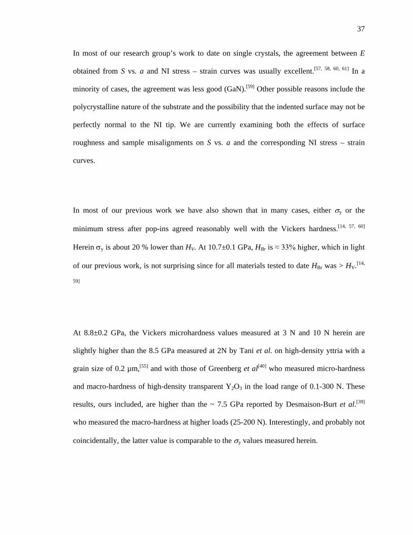
As shown in Fig. 3.3, EBr is a function of penetration depth. Thus the average value obtained

will depend on range chosen. In the 100 nm ≤ htot ≤ 1500 nm range, the average EBr = 178±3;

if the range is restricted to the flatter 500 nm ≤ htot ≤ 1500 nm range, the average EBr = 185±3

GPa. The former is 1 % higher than ES; the latter is 5 % higher.

30

Table 3-1: Summary of E values measured using the various methods explored in this work. For the spherical NI, the S vs. a slopes were zero corrected and forced through the origin.[34] The maximum loads used for the measurements were 50 mN and 80 mN for 1.4 µm and 5 µm tips, respectively.

Method Remarks E (GPa)

1.4 μm 5 μm

M1 S vs. a, up to limit of spherical radii viz. 0.8 µm, 1.7 µm for the 1.4 and 5 µm indenters, respectively.

168±3 158±3

M2 S vs. a, up to yield point 171±2 170±7

Berkovich Penetration depth range 100 to 1500 nm (Fig. 3.3) 178±3

Penetration depth range 500 to 1500 nm (Fig. 3.3) 185±3

Dynamic elastic modulus 176.2±1.7

Fig. 3-3: Dependence of EBr on depth-of-indentation into 7 different locations. The average value of EBr depends on the range of penetration. In the 100 nm to 1500 nm range least squares fits yields EBr = 178±3 GPa; in the 500 nm to 1500 nm range, EBr = 185±3 GPa. Note that at the intercept of the two thick dashed lines EBr is about 170 GPa.

31

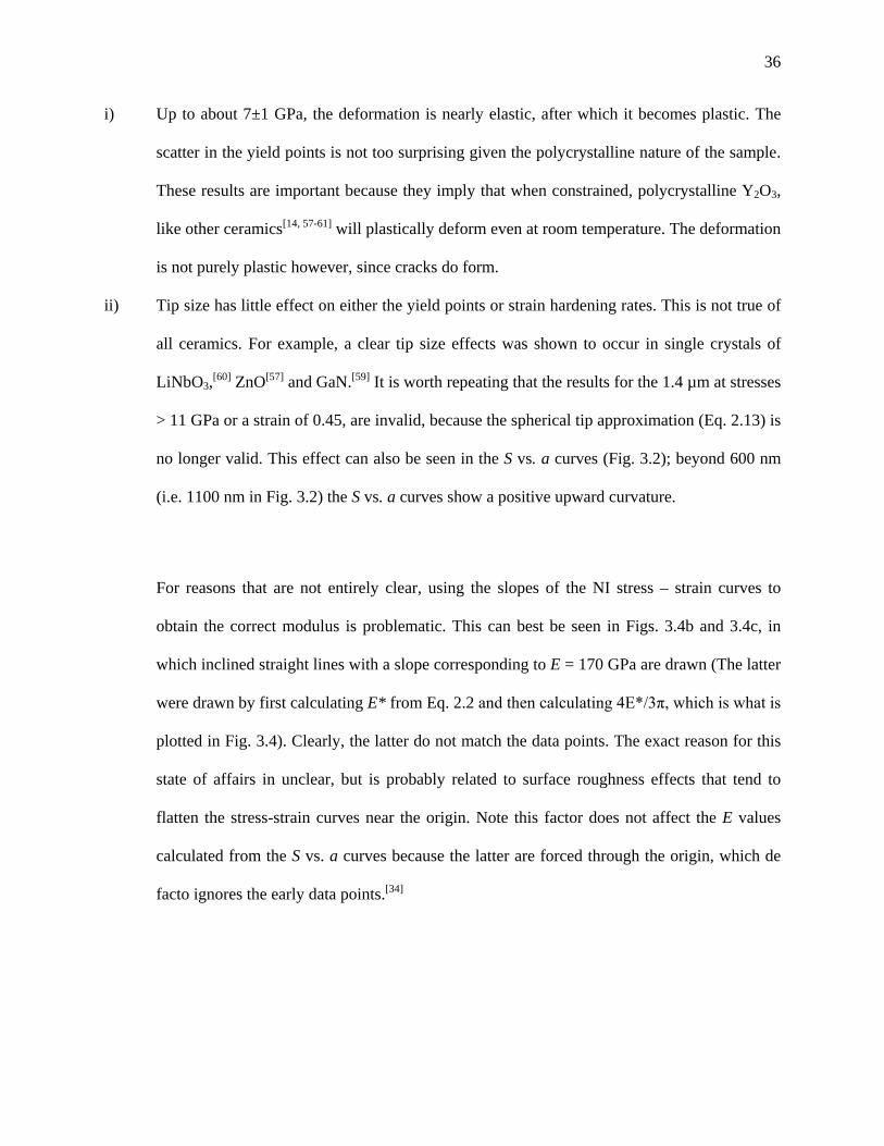
3.4.3. NI Stress-Strain Curves

Typical load – displacement curves for both spherical tips are compared in Fig. 3.4a; the

corresponding NI stress – strain curves for select locations for the 5 µm and 1.4 µm tips are

shown in Figs. 3.4b and 3.4c, respectively. For comparison purposes, the NI stress – strain

curves of one of the locations plotted in Fig. 3.4b is reproduced (open red diamonds) in Fig.

3.4c. It follows that the hardening rates for both tips are comparable.

At 7±1 GPa, the average σy for the two tips are statistically identical. (6.9±0.9 and 7.2±0.4

GPa for the 1.4 µm and 5 µm tip radii, respectively). The stress at which the NI stress – strain

curves, above and below the yield points intersected was taken to be σy. The maximum stress,

σmax, attained using the 5 µm tip size is 9±0.2 GPa, at a strain, ε ~ 0.3. For the 1.4 µm tip,

σmax, is 14±1 GPa at a ε ~ 0.7. However, as mentioned above and discussed below, the results

beyond ε ~ 0.5 are invalid since it is at that strain that the tip is no longer spherical, but

becomes conical. The upturn in the work-hardening rate at ε > 0.5 – where a > 800 nm - is a

reflection of this fact.

32

Fig. 3-4: a) Typical load – displacement curves, from multiple locations, for the two tips. Note excellent reproducibility from location to location. The width of the inset = 50 µm. b) Typical NI stress – strain curves for the 5 µm tip and, c) 1.4 µm tip. Dashed inclined lines going through the origin represent the expected stress-strain trajectory assuming a modulus of 170 GPa.

3.4.4. Hardness and Fracture Toughness

The average HBr and HV, values were calculated to be 10.7±0.1 GPa and 8.8±0.2 GPa,

respectively. The same HV values were obtained at 3 N and 10 N. Short horizontal lines,

33

labeled HV, and HBr, appear near the y-axis in Fig. 3.4c. Clearly, the order of the hardness

values is HBr > HV > σy.

The K1C values calculated - using Eqs. 2.19-2.23 listed in Table 2.1, ranged from 1.2 to 1.8

MPam1/2. Calculated results are shown in Table 3.2.

Table 3-2: Calculated K1C values of Y2O3 at the loads of 3N and 10N.

Method K1C (MPam1/2)

(3 N)

K1C (MPam1/2)

(10 N) Equation #

Anstis et al.[7] 1.4±0.1 1.3±0.1 (2.19)

Niihara et al.[8] 1.8±0.1 1.7±0.1 (2.20)

Evans & Charles[9] 1.3±0.1 1.2±0.1 (2.21)

Laugier[10] 1.3±0.1 1.2±0.1 (2.22)

Lankford[11] 1.8±0.2 1.7±0.1 (2.23)

3.4.5. OM and SEM Results

Typical SEM micrographs of the 1.4 µm and 5 µm indentation marks formed at loads of 50

mN and 80 mN are shown in Figs. 3.5a and 3.5b, respectively. From these results it is

obvious that the spherical NI introduces more, but smaller, cracks than the Vickers indent

34

shown in Fig. 3.5c imaged using an OM. The push out of a few grains around the perimeter

of the spherical NI is noteworthy.

Fig. 3-5: Typical SEM micrographs of indentation mark made on the surface with, a) the 1.4 µm loaded to 50 mN and b) 5 µm loaded to 80 mN. Note small cracks emanating from the edges and the pushing out of a number of small grains along the periphery of the indentation. An OM image of a Vickers indent at a 3N load is shown in (c).

35

3.5. Discussion

3.5.1. Elastic Moduli

The ES obtained herein, 176±1.7 GPa, is in good agreement with the value of 173±2 GPa,

calculated by Palko et al.[62] A perusal of Table 3.1 indicates that using method M1, for the

1.4 µm and 5 µm tips results in ESp which underestimate ES by ~ 3% and ~10%, respectively.

The reasons for this tip size dependence is unclear, but may be attributed to the differences in

crack sizes that form under the various indenters. From Fig. 3.5a and 3.5b, the crack size for

the 1.4 µm and 5 µm indenters are roughly 1 µm and 5.5 µm, respectively. Supporting this

notion is the fact that when the S vs. a results are restricted to the elastic regime (method

M2), where presumably no cracks form, ESp of both tips are identical and underestimate ES

by only ~ 3%. This small underestimation, notwithstanding, the fact that the average values

for both tips are in excellent agreement with each other, and their proximity to ES is

gratifying. As importantly, these values are closer to E than the Young's moduli measured in

compression tests on 99.7 % dense Y2O3, that are in the vicinity 150 GPa.[54] The EBr

overestimates ES by ≈ 1% to 5 % depending on indentation depth range considered (see Fig.

3.3 and Table 3.1).

3.5.2. NI Stress – Strain Curves

An obvious advantage of using spherical indenters, however, is the ability to obtain NI stress

– strain curves. From the results shown in Figs. 3.4b and 3.4c it is reasonable to conclude

that:

36

i) Up to about 7±1 GPa, the deformation is nearly elastic, after which it becomes plastic. The

scatter in the yield points is not too surprising given the polycrystalline nature of the sample.

These results are important because they imply that when constrained, polycrystalline Y2O3,

like other ceramics[14, 57-61] will plastically deform even at room temperature. The deformation

is not purely plastic however, since cracks do form.

ii) Tip size has little effect on either the yield points or strain hardening rates. This is not true of

all ceramics. For example, a clear tip size effects was shown to occur in single crystals of

LiNbO3,[60] ZnO[57] and GaN.[59] It is worth repeating that the results for the 1.4 µm at stresses

> 11 GPa or a strain of 0.45, are invalid, because the spherical tip approximation (Eq. 2.13) is

no longer valid. This effect can also be seen in the S vs. a curves (Fig. 3.2); beyond 600 nm

(i.e. 1100 nm in Fig. 3.2) the S vs. a curves show a positive upward curvature.

For reasons that are not entirely clear, using the slopes of the NI stress – strain curves to

obtain the correct modulus is problematic. This can best be seen in Figs. 3.4b and 3.4c, in

which inclined straight lines with a slope corresponding to E = 170 GPa are drawn (The latter

were drawn by first calculating E* from Eq. 2.2 and then calculating 4E*/3π, which is what is

plotted in Fig. 3.4). Clearly, the latter do not match the data points. The exact reason for this

state of affairs in unclear, but is probably related to surface roughness effects that tend to

flatten the stress-strain curves near the origin. Note this factor does not affect the E values

calculated from the S vs. a curves because the latter are forced through the origin, which de

facto ignores the early data points.[34]

37

In most of our research group’s work to date on single crystals, the agreement between E

obtained from S vs. a and NI stress – strain curves was usually excellent.[57, 58, 60, 61] In a

minority of cases, the agreement was less good (GaN).[59] Other possible reasons include the

polycrystalline nature of the substrate and the possibility that the indented surface may not be

perfectly normal to the NI tip. We are currently examining both the effects of surface

roughness and sample misalignments on S vs. a and the corresponding NI stress – strain

curves.

In most of our previous work we have also shown that in many cases, either σy or the

minimum stress after pop-ins agreed reasonably well with the Vickers hardness.[14, 57, 60]

Herein σy is about 20 % lower than HV. At 10.7±0.1 GPa, HBr is ≈ 33% higher, which in light

of our previous work, is not surprising since for all materials tested to date HBr was > HV.[14,

59]

At 8.8±0.2 GPa, the Vickers microhardness values measured at 3 N and 10 N herein are

slightly higher than the 8.5 GPa measured at 2N by Tani et al. on high-density yttria with a

grain size of 0.2 µm,[55] and with those of Greenberg et al[40] who measured micro-hardness

and macro-hardness of high-density transparent Y2O3 in the load range of 0.1-300 N. These

results, ours included, are higher than the ~ 7.5 GPa reported by Desmaison-Burt et al.[39]

who measured the macro-hardness at higher loads (25-200 N). Interestingly, and probably not

coincidentally, the latter value is comparable to the σy values measured herein.

38

The average K1C of all the methods listed in Table 2.1 is 1.5±0.3 MPam1/2. These results are

consistent with the results of Desmaison-Burt et al. who measured K1C on high-density Y2O3

using various methods.[39] The K1C values reported were in the 1.2 – 1.8 MPam1/2 range

depending on equation used.

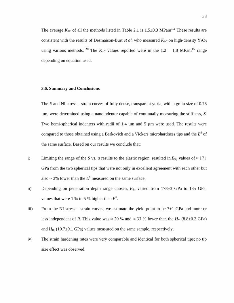
3.6. Summary and Conclusions

The E and NI stress – strain curves of fully dense, transparent yttria, with a grain size of 0.76

µm, were determined using a nanoindenter capable of continually measuring the stiffness, S.

Two hemi-spherical indenters with radii of 1.4 µm and 5 µm were used. The results were

compared to those obtained using a Berkovich and a Vickers microhardness tips and the ES of

the same surface. Based on our results we conclude that:

i) Limiting the range of the S vs. a results to the elastic region, resulted in ESp values of ≈ 171

GPa from the two spherical tips that were not only in excellent agreement with each other but

also ~ 3% lower than the ES measured on the same surface.

ii) Depending on penetration depth range chosen, EBr varied from 178±3 GPa to 185 GPa;

values that were 1 % to 5 % higher than ES.

iii) From the NI stress – strain curves, we estimate the yield point to be 7±1 GPa and more or

less independent of R. This value was ≈ 20 % and ≈ 33 % lower than the HV (8.8±0.2 GPa)

and HBr (10.7±0.1 GPa) values measured on the same sample, respectively.

iv) The strain hardening rates were very comparable and identical for both spherical tips; no tip

size effect was observed.

39

v) At 1.5±0.3 MPam1/2, the fracture toughness values extracted from the Vickers microhardness

indentations are in good agreement with published results on samples with comparable

microstructures.

40

Chapter 4 : MECHANICAL PROPERTIES OF SCANDIA and ERBIA: THE EFFECT OF POLISHING QUALITY and SURFACE ROUGHNESS

4.1. Introduction

Scandium oxide, (scandia, Sc2O3), a cubic sesquioxide that resembles the light elements in

the binary rare earth sesquioxide (R2O3) ceramics[53] - is sometimes considered for high

temperature applications [51] It is also considered as a host material for solid lasers,[63-65] and

as heat-resistant optical windows in solid state laser.[65] Erbium oxide, (erbia, Er2O3), is also a

cubic material with high stability and corrosion resistance.[66, 67]

Data on the E and strengths of Sc2O3 are scarce[51, 68] and so are the elastic and mechanical

properties of Er2O3.[66, 67, 69] For 98.7% dense Sc2O3, Gogotsi reported that the E ranged from

218 to 251 GPa.[51] He also claimed that E determined from 4-point flexure experiments

depended on sample size.[51, 70] Dole et al. report the ES of slightly porous Sc2O3 and based on

a linear relationship between the E and the volume fraction of pores they estimated a value of

227 GPa for pore free material.[68]

The E and K1C values of Sc2O3 and Er2O3 were recently revisited. Gogotsi et al., based on his

previous study on Sc2O3,[51] reported an E value of 218 GPa.[70] The bulk moduli, B, can be

either measured isothermally, or by dynamic methods or even can be estimated based on

various calculation procedures. From the physical point of view, B of various R2O3

41

compounds were evaluated by various estimation methods based on the interatomic distance.

According to these procedures B of Sc2O3 ranges from 126 to 167 GPa.[71] The isothermal B

obtained from a diamond anvil cell pressurized to 31 GPa yielded a value of 189±7 GPa.[72]

Yusa et al.[72] calculated an even higher B value, 199 GPa, while Barzilai et al. calculated a B

of 174.5±1 GPa.[73] Based on the reported B values and on the known v of fully dense Sc2O3,

viz. 0.256,[68] the calculated E are in the range of 250±41 GPa. This ~ 16 % scatter is

unacceptable for the E of any material.

For Er2O3 the E of porous samples, measured by Manning et al. and then extrapolated to full

density, was reported to be ~175 GPa.[74] Lately, the elastic constants of single crystals were

measured and the calculated E values of polycrystalline samples from the elastic constants

was reported to be ~ 177 GPa.[69]

The objective of this chapter is to characterize the room-temperature mechanical properties of

fully dense Sc2O3 and Er2O3 using the technique described in Ch. 2 and to compare the

results with other more established hardness techniques, such as Vickers and Berkovich. The

present study focuses on NI stress – strain curves on nearly fully dense Sc2O3 and slightly

porous Er2O3, with grain sizes of about 1 µm and 3 µm, respectively. We compared the E

determined by the method detailed in Ch. 2 to the ES measured by ultrasound on the same

sample. The HV and K1C were also measured for both of the materials.

42

4.2. Experimental Details

4.2.1. Sample Processing

A 99.99% pure Sc2O3 powder (China Rare Metals Material Co. Ltd, China) with an average

particle size of < 1 µm, was cold isostatically pressed at 300 MPa. The compacts were heat-

treated using a proprietary treatment in air, followed by annealing for 24 hours in vacuum (~

3 Pa) to dry them. The pressed and treated compact was then hot isostatically pressed

(HIPed) at 1300°C under a pressure of 130 MPa for 5 hours. For Er2O3, a 99.95% pure

powder was compacted and followed the same procedure as the yttria samples consolidated

by HIP.[42]

A ≈ 8 mm thick slice of Sc2O3 and a ≈ 2.7 mm slice of Er2O3 were used in the present study.

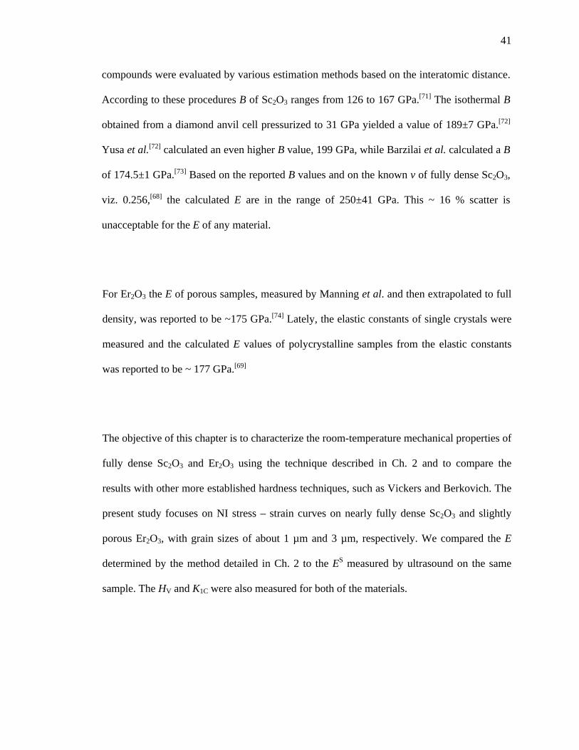
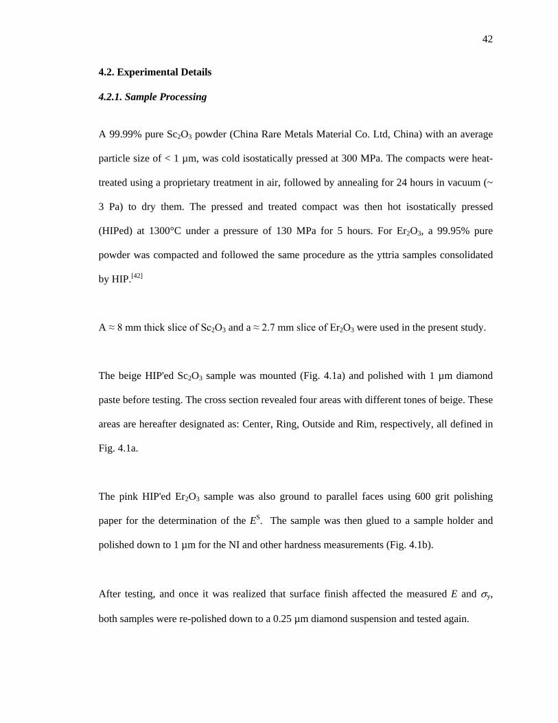
The beige HIP'ed Sc2O3 sample was mounted (Fig. 4.1a) and polished with 1 µm diamond

paste before testing. The cross section revealed four areas with different tones of beige. These

areas are hereafter designated as: Center, Ring, Outside and Rim, respectively, all defined in

Fig. 4.1a.

The pink HIP'ed Er2O3 sample was also ground to parallel faces using 600 grit polishing

paper for the determination of the ES. The sample was then glued to a sample holder and

polished down to 1 µm for the NI and other hardness measurements (Fig. 4.1b).

After testing, and once it was realized that surface finish affected the measured E and σy,

both samples were re-polished down to a 0.25 µm diamond suspension and tested again.

43

Fig. 4-1: a) The mounted Sc2O3 sample with four tones of beige in the areas which were measure in the present study; Edge, Outside, Ring and Center. b) The polished Er2O3 sample fixed on the sample holder.

4.2.2. Material Characterization

4.2.2.1. Dynamic Elastic Modulus

ES and ρ were measured by the method explained in Ch. 2. The uncertainty in the density

measurements is estimated to be ≈ ± 0.1%; that in VL ≈ ± 0.1%, and that in VT ≈ ± 0.1%. The

resulting uncertainty in ES is thus better than 1%, vS is about 3%.

44

4.2.2.2. Vickers Microhardness

A microhardness tester was used to measure the Vickers microhardness. Six indents in all of

the regions of Sc2O3 sample, - a total 24 indents - were made using a 3 N load and a 15 s

dwell time. Their average value was used as the final Vickers microhardness value of Sc2O3.

A total six indents on Er2O3 were made using the same parameters.

4.2.2.3. Optical Microscopy and Scanning Electron Microscopy

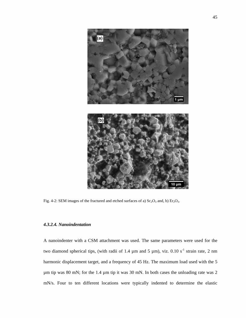
To measure the grain size, fractured surfaces were etched by immersing them in boiling

H2SO4 for 20s. The average grain size was determined using the line-intercept method of ≈

20 and 40 grains for Sc2O3 and Er2O3, respectively. Figures 4.2a and 4.2b show SEM

micrographs of fractured and etched surfaces of Sc2O3 and Er2O3, respectively.

An OM and a SEM were used to image the polished surfaces before and after the various

indentations.

45

Fig. 4-2: SEM images of the fractured and etched surfaces of a) Sc2O3 and, b) Er2O3.

4.3.2.4. Nanoindentation

A nanoindenter with a CSM attachment was used. The same parameters were used for the

two diamond spherical tips, (with radii of 1.4 µm and 5 µm), viz. 0.10 s-1 strain rate, 2 nm

harmonic displacement target, and a frequency of 45 Hz. The maximum load used with the 5

µm tip was 80 mN; for the 1.4 µm tip it was 30 mN. In both cases the unloading rate was 2

mN/s. Four to ten different locations were typically indented to determine the elastic

46

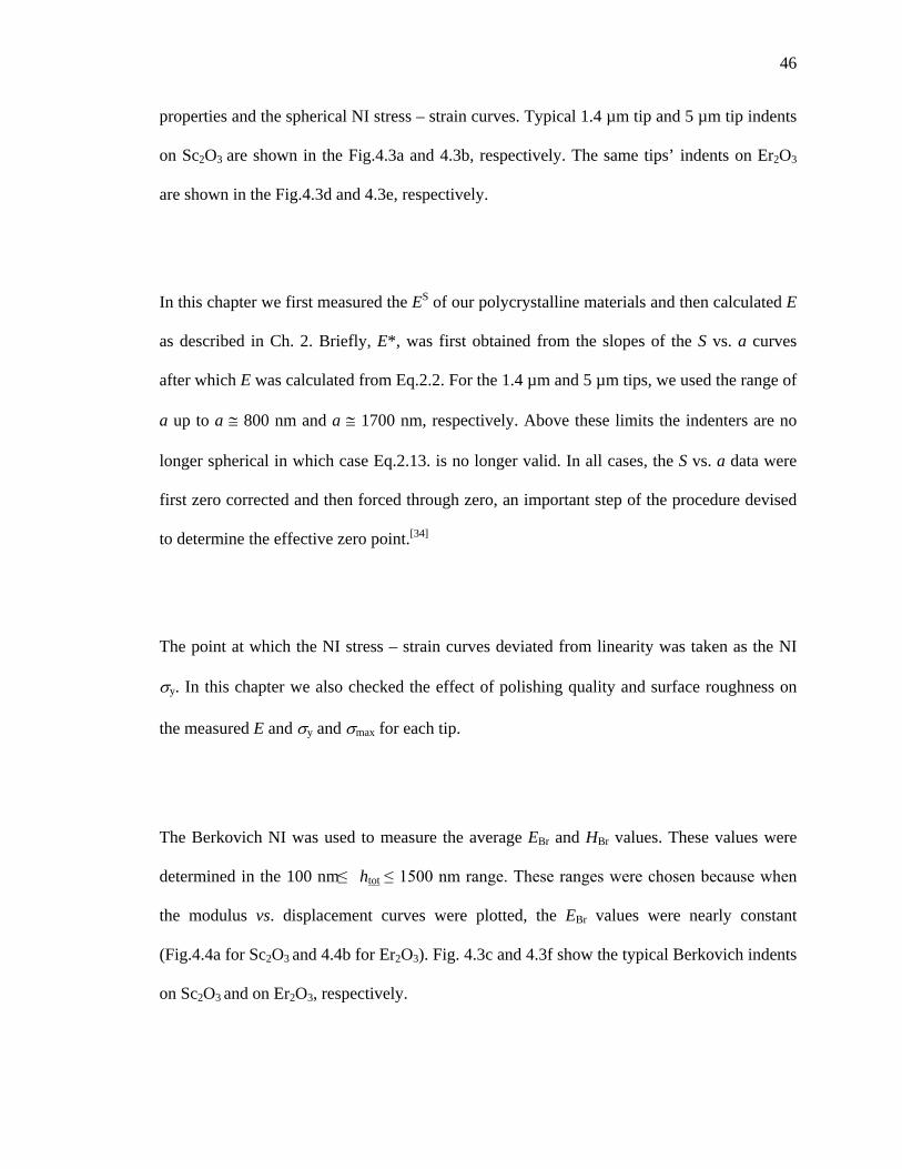
properties and the spherical NI stress – strain curves. Typical 1.4 µm tip and 5 µm tip indents

on Sc2O3 are shown in the Fig.4.3a and 4.3b, respectively. The same tips’ indents on Er2O3

are shown in the Fig.4.3d and 4.3e, respectively.

In this chapter we first measured the ES of our polycrystalline materials and then calculated E

as described in Ch. 2. Briefly, E*, was first obtained from the slopes of the S vs. a curves

after which E was calculated from Eq.2.2. For the 1.4 µm and 5 µm tips, we used the range of

a up to a ≅ 800 nm and a ≅ 1700 nm, respectively. Above these limits the indenters are no

longer spherical in which case Eq.2.13. is no longer valid. In all cases, the S vs. a data were

first zero corrected and then forced through zero, an important step of the procedure devised

to determine the effective zero point.[34]

The point at which the NI stress – strain curves deviated from linearity was taken as the NI

σy. In this chapter we also checked the effect of polishing quality and surface roughness on

the measured E and σy and σmax for each tip.

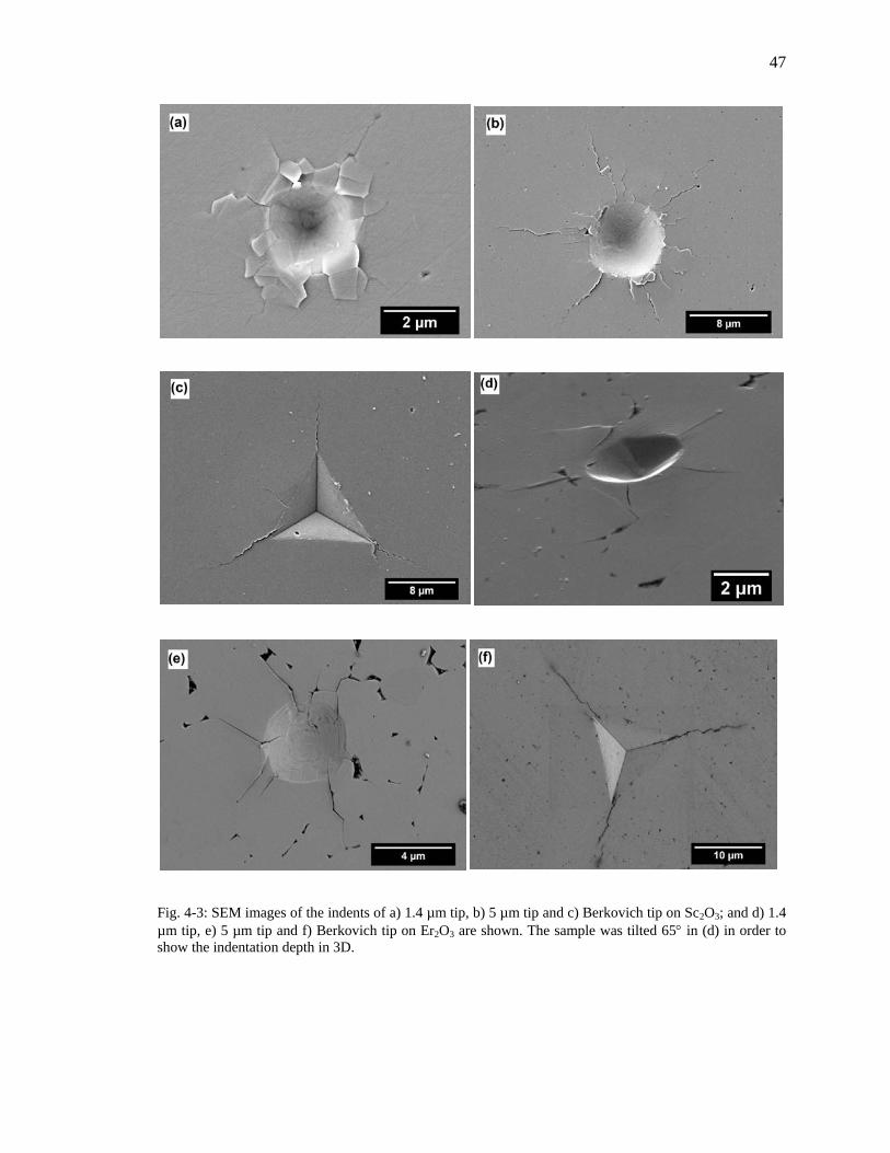
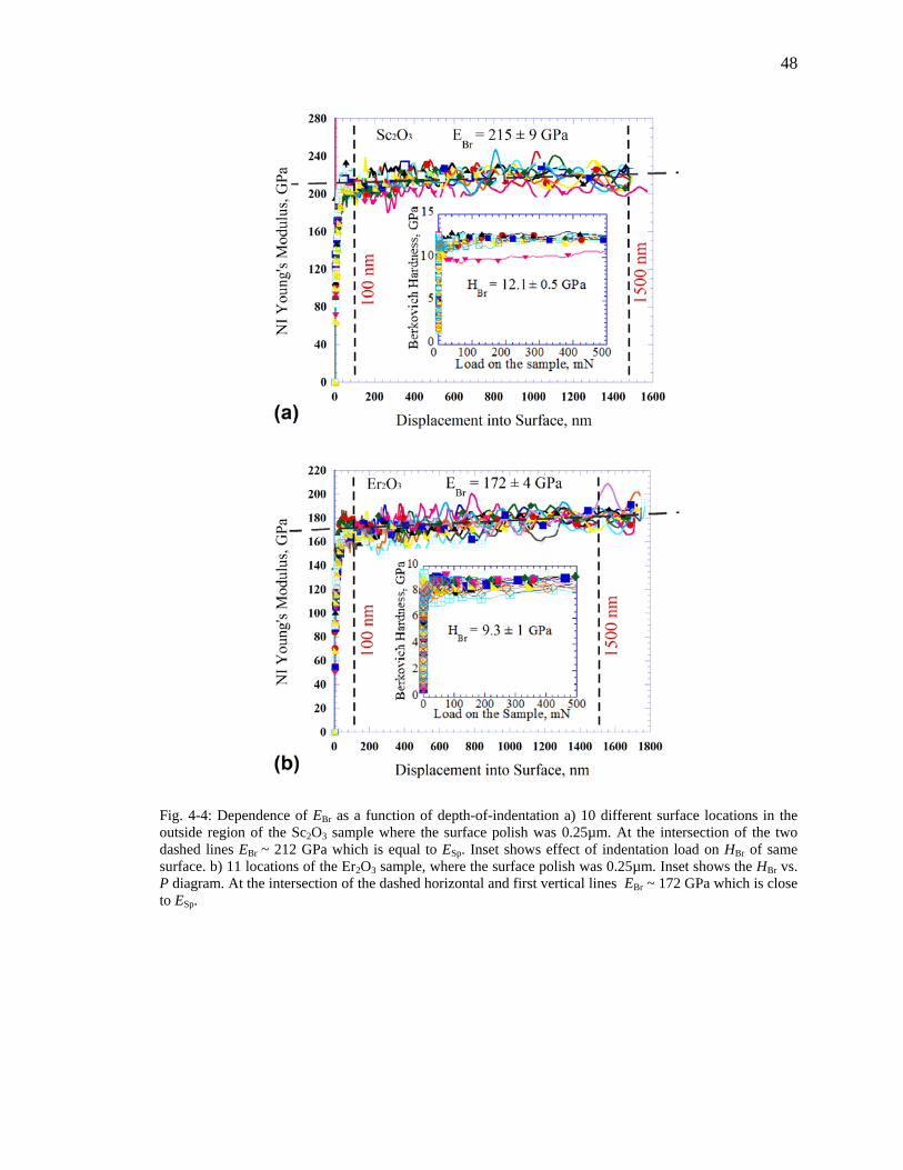
The Berkovich NI was used to measure the average EBr and HBr values. These values were

determined in the 100 nm ≤ htot

≤ 1500 nm range. These ranges were chosen because when

the modulus vs. displacement curves were plotted, the EBr values were nearly constant

(Fig.4.4a for Sc2O3 and 4.4b for Er2O3). Fig. 4.3c and 4.3f show the typical Berkovich indents

on Sc2O3 and on Er2O3, respectively.

47

Fig. 4-3: SEM images of the indents of a) 1.4 µm tip, b) 5 µm tip and c) Berkovich tip on Sc2O3; and d) 1.4 µm tip, e) 5 µm tip and f) Berkovich tip on Er2O3 are shown. The sample was tilted 65° in (d) in order to show the indentation depth in 3D.

48

Fig. 4-4: Dependence of EBr as a function of depth-of-indentation a) 10 different surface locations in the outside region of the Sc2O3 sample where the surface polish was 0.25µm. At the intersection of the two dashed lines EBr ~ 212 GPa which is equal to ESp. Inset shows effect of indentation load on HBr of same surface. b) 11 locations of the Er2O3 sample, where the surface polish was 0.25µm. Inset shows the HBr vs. P diagram. At the intersection of the dashed horizontal and first vertical lines EBr ~ 172 GPa which is close to ESp.

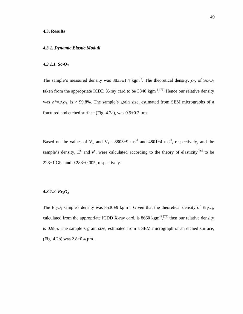
49

4.3. Results

4.3.1. Dynamic Elastic Moduli

4.3.1.1. Sc2O3

The sample’s measured density was 3833±1.4 kgm-3. The theoretical density, ρT, of Sc2O3

taken from the appropriate ICDD X-ray card to be 3840 kgm-3.[75] Hence our relative density

was ρ*=ρ/ρT, is > 99.8%. The sample’s grain size, estimated from SEM micrographs of a

fractured and etched surface (Fig. 4.2a), was 0.9±0.2 µm.

Based on the values of VL and VT - 8803±9 ms-1 and 4801±4 ms-1, respectively, and the

sample’s density, ES and vS, were calculated according to the theory of elasticity[76] to be

228±1 GPa and 0.288±0.005, respectively.

4.3.1.2. Er2O3

The Er2O3 sample's density was 8530±9 kgm-3. Given that the theoretical density of Er2O3,

calculated from the appropriate ICDD X-ray card, is 8660 kgm-3,[75] then our relative density

is 0.985. The sample’s grain size, estimated from a SEM micrograph of an etched surface,

(Fig. 4.2b) was 2.8±0.4 µm.

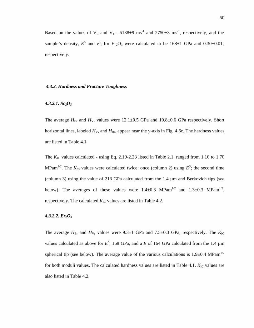
50

Based on the values of VL and VT - 5138±9 ms-1 and 2750±3 ms-1, respectively, and the

sample’s density, ES and vS, for Er2O3 were calculated to be 168±1 GPa and 0.30±0.01,

respectively.

4.3.2. Hardness and Fracture Toughness

4.3.2.1. Sc2O3

The average HBr and HV, values were 12.1±0.5 GPa and 10.8±0.6 GPa respectively. Short

horizontal lines, labeled HV, and HBr, appear near the y-axis in Fig. 4.6c. The hardness values

are listed in Table 4.1.

The KIC values calculated - using Eq. 2.19-2.23 listed in Table 2.1, ranged from 1.10 to 1.70

MPam1/2. The KIC values were calculated twice: once (column 2) using ES; the second time

(column 3) using the value of 213 GPa calculated from the 1.4 µm and Berkovich tips (see

below). The averages of these values were 1.4±0.3 MPam1/2 and 1.3±0.3 MPam1/2,

respectively. The calculated KIC values are listed in Table 4.2.

4.3.2.2. Er2O3

The average HBr and HV, values were 9.3±1 GPa and 7.5±0.3 GPa, respectively. The KIC

values calculated as above for ES, 168 GPa, and a E of 164 GPa calculated from the 1.4 µm

spherical tip (see below). The average value of the various calculations is 1.9±0.4 MPam1/2

for both moduli values. The calculated hardness values are listed in Table 4.1. KIC values are

also listed in Table 4.2.

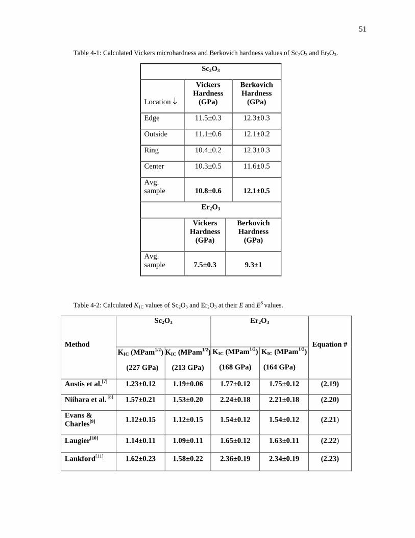
51

Table 4-1: Calculated Vickers microhardness and Berkovich hardness values of Sc2O3 and Er2O3.

Sc2O3

Location ↓

Vickers Hardness

(GPa)

Berkovich Hardness

(GPa)

Edge 11.5±0.3 12.3±0.3

Outside 11.1±0.6 12.1±0.2

Ring 10.4±0.2 12.3±0.3

Center 10.3±0.5 11.6±0.5

Avg. sample 10.8±0.6 12.1±0.5

Er2O3

Vickers Hardness

(GPa)

Berkovich Hardness

(GPa)

Avg. sample 7.5±0.3 9.3±1

Table 4-2: Calculated K1C values of Sc2O3 and Er2O3 at their E and ES values.

Method

Sc2O3

Er2O3

Equation #

KIC (MPam1/2)

(227 GPa)

KIC (MPam1/2)

(213 GPa)

KIC (MPam1/2)

(168 GPa)

KIC (MPam1/2)

(164 GPa)

Anstis et al.[7] 1.23±0.12 1.19±0.06 1.77±0.12 1.75±0.12 (2.19)

Niihara et al. [8] 1.57±0.21 1.53±0.20 2.24±0.18 2.21±0.18 (2.20)

Evans & Charles[9] 1.12±0.15 1.12±0.15 1.54±0.12 1.54±0.12 (2.21)

Laugier[10] 1.14±0.11 1.09±0.11 1.65±0.12 1.63±0.11 (2.22)

Lankford[11] 1.62±0.23 1.58±0.22 2.36±0.19 2.34±0.19 (2.23)

52

4.3.3. Moduli Obtained from the S vs a Curves

4.3.3.1. Sc2O3

The S vs. a curves - for the 1.4 µm and 5 µm indenters, for both surface finishes - shown in

Fig. 4.5a confirm that the relationship between S vs. a is linear. The reproducibility of the

curves in the various locations is noteworthy. The main effect of polishing was in slightly

changing the curvatures near the origin. The calculated E values, for both tips and surface

finishes, using the S vs. a method are listed in Table 4.3. Clearly both indenter tip size and

surface finishes affect the moduli values.

4.3.3.2. Er2O3

The S vs. a curves - for the 1.4 µm and 5 µm indenters, for both surface finishes - shown in

Fig. 4.5b again confirm that the relationship between S vs. a is linear. Here again, the

reproducibility of the curves in the various locations is noteworthy. In this case, the curvature

near the origin for the 5 µm indenter in surfaces polished down to 0.25 µm is reduced as

compared to the surfaces polished down to 1 µm.

The calculated E values, for both tips and surface finishes, using the S vs. a method are listed

in Table 4.3. Clearly both indenter tip size and surface finish affect the moduli values.

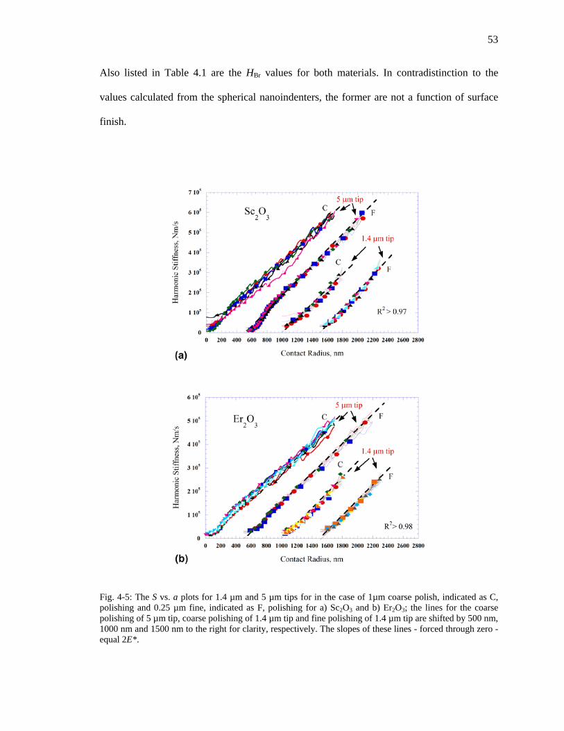
53

Also listed in Table 4.1 are the HBr values for both materials. In contradistinction to the

values calculated from the spherical nanoindenters, the former are not a function of surface

finish.

Fig. 4-5: The S vs. a plots for 1.4 µm and 5 µm tips for in the case of 1µm coarse polish, indicated as C, polishing and 0.25 µm fine, indicated as F, polishing for a) Sc2O3 and b) Er2O3; the lines for the coarse polishing of 5 µm tip, coarse polishing of 1.4 µm tip and fine polishing of 1.4 µm tip are shifted by 500 nm, 1000 nm and 1500 nm to the right for clarity, respectively. The slopes of these lines - forced through zero - equal 2E*.

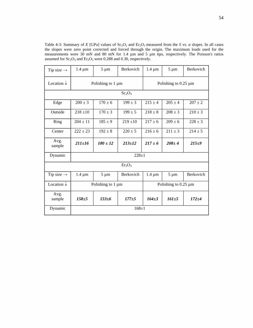
54

Table 4-3: Summary of E [GPa] values of Sc2O3 and Er2O3 measured from the S vs. a slopes. In all cases the slopes were zero point corrected and forced through the origin. The maximum loads used for the measurements were 30 mN and 80 mN for 1.4 µm and 5 µm tips, respectively. The Poisson's ratios assumed for Sc2O3 and Er2O3 were 0.288 and 0.30, respectively.

Tip size → 1.4 µm 5 µm Berkovich 1.4 µm 5 µm Berkovich

Location ↓ Polishing to 1 µm Polishing to 0.25 µm

Sc2O3

Edge 200 ± 3 170 ± 6 199 ± 3 215 ± 4 205 ± 4 207 ± 2

Outside 218 ±10 170 ± 3 199 ± 5 218 ± 8 208 ± 3 210 ± 3

Ring 204 ± 11 185 ± 9 219 ±10 217 ± 6 209 ± 6 228 ± 3

Center 222 ± 23 192 ± 8 220 ± 5 216 ± 6 211 ± 3 214 ± 5

Avg. sample 211±16 180 ± 12 213±12 217 ± 6 208± 4 215±9

Dynamic 228±1

Er2O3

Tip size → 1.4 µm 5 µm Berkovich 1.4 µm 5 µm Berkovich

Location ↓ Polishing to 1 µm Polishing to 0.25 µm

Avg. sample 158±5 153±6 177±5 164±3 161±5 172±4

Dynamic 168±1

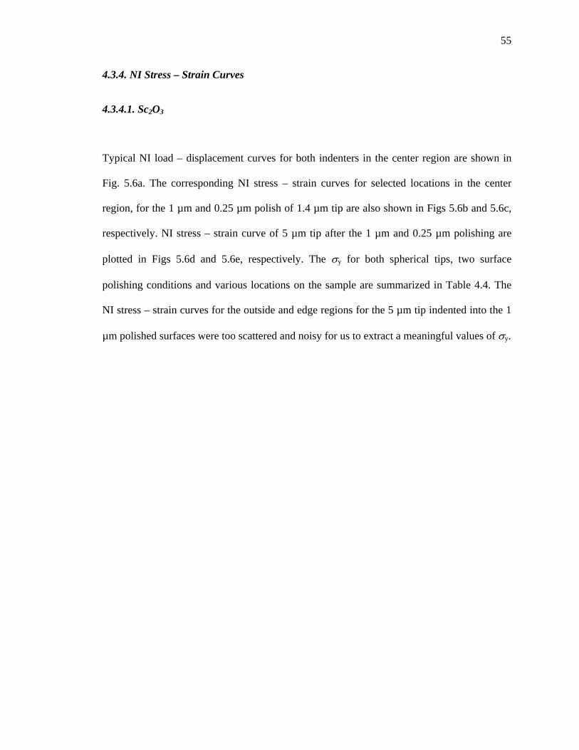
55

4.3.4. NI Stress – Strain Curves

4.3.4.1. Sc2O3

Typical NI load – displacement curves for both indenters in the center region are shown in

Fig. 5.6a. The corresponding NI stress – strain curves for selected locations in the center

region, for the 1 µm and 0.25 µm polish of 1.4 µm tip are also shown in Figs 5.6b and 5.6c,

respectively. NI stress – strain curve of 5 µm tip after the 1 µm and 0.25 µm polishing are

plotted in Figs 5.6d and 5.6e, respectively. The σy for both spherical tips, two surface

polishing conditions and various locations on the sample are summarized in Table 4.4. The

NI stress – strain curves for the outside and edge regions for the 5 µm tip indented into the 1

µm polished surfaces were too scattered and noisy for us to extract a meaningful values of σy.

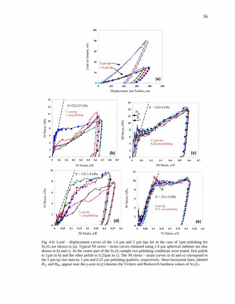
56

Fig. 4-6: Load – displacement curves of the 1.4 µm and 5 µm tips for in the case of 1µm polishing for Sc2O3 are shown in (a). Typical NI stress – strain curves obtained using 1.4 µm spherical indenter are also shown in b) and c). At the center part of the Sc2O3 sample two polishing conditions were tested, first polish to 1µm in b) and the other polish to 0.25µm in c). The NI stress – strain curves in d) and e) correspond to the 5 µm tip size data by 1 µm and 0.25 µm polishing qualities, respectively. Short horizontal lines, labeled HV, and HBr, appear near the y-axis in (c) denotes the Vickers and Berkovich hardness values of Sc2O3.

57

4.3.4.2. Er2O3

Typical NI load – displacement curves for both indenters are shown in Fig. 4.7a. The

corresponding NI stress-strain curves by 1 µm tip in various locations across the 1 µm and

0.25 µm polishing appear in Figs 4.7b and 4.7c, respectively. Indentation stress-strain curves

of 5 µm tip by 1 µm and 0.25 µm polishing conditions are plotted in Figs 5.7d and 5.7e,

respectively. The σy for both spherical tips and two surface polishing conditions are

summarized in Table 4.4.

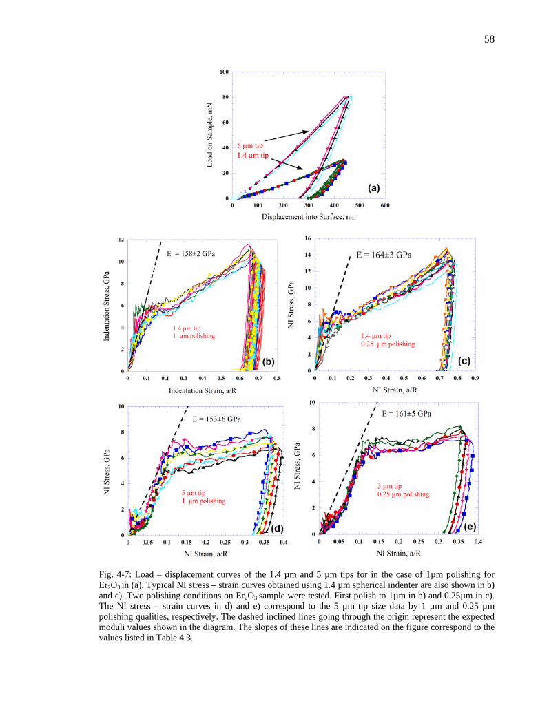
58

Fig. 4-7: Load – displacement curves of the 1.4 µm and 5 µm tips for in the case of 1µm polishing for Er2O3 in (a). Typical NI stress – strain curves obtained using 1.4 µm spherical indenter are also shown in b) and c). Two polishing conditions on Er2O3 sample were tested. First polish to 1µm in b) and 0.25µm in c). The NI stress – strain curves in d) and e) correspond to the 5 µm tip size data by 1 µm and 0.25 µm polishing qualities, respectively. The dashed inclined lines going through the origin represent the expected moduli values shown in the diagram. The slopes of these lines are indicated on the figure correspond to the values listed in Table 4.3.

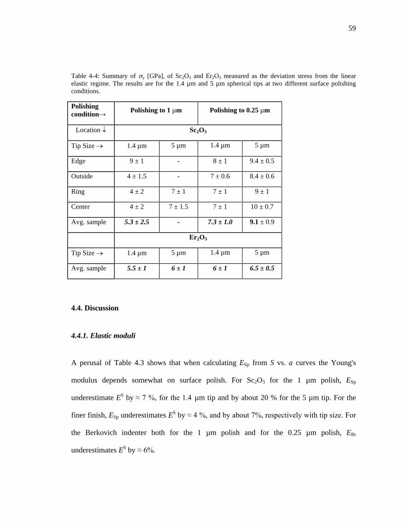
59

Table 4-4: Summary of σy [GPa], of Sc2O3 and Er2O3 measured as the deviation stress from the linear elastic regime. The results are for the 1.4 µm and 5 µm spherical tips at two different surface polishing conditions.

Polishing condition→ Polishing to 1 µm Polishing to 0.25 µm

Location ↓ Sc2O3

Tip Size → 1.4 µm 5 µm 1.4 µm 5 µm

Edge 9 ± 1 - 8 ± 1 9.4 ± 0.5

Outside 4 ± 1.5 - 7 ± 0.6 8.4 ± 0.6

Ring 4 ± 2 7 ± 1 7 ± 1 9 ± 1

Center 4 ± 2 7 ± 1.5 7 ± 1 10 ± 0.7

Avg. sample 5.3 ± 2.5 - 7.3 ± 1.0 9.1 ± 0.9

Er2O3

Tip Size → 1.4 µm 5 µm 1.4 µm 5 µm

Avg. sample 5.5 ± 1 6 ± 1 6 ± 1 6.5 ± 0.5

4.4. Discussion

4.4.1. Elastic moduli

A perusal of Table 4.3 shows that when calculating ESp from S vs. a curves the Young's

modulus depends somewhat on surface polish. For Sc2O3 for the 1 µm polish, ESp

underestimate ES by ≈ 7 %, for the 1.4 µm tip and by about 20 % for the 5 µm tip. For the

finer finish, ESp underestimates ES by ≈ 4 %, and by about 7%, respectively with tip size. For

the Berkovich indenter both for the 1 µm polish and for the 0.25 µm polish, EBr

underestimates ES by ≈ 6%.

60

For the Er2O3, ESp underestimates ES for both surface finish conditions, with an effect of tip

size. The EBr, however overestimates ES by about 6% and 2.5% for the 1 µm and 0.25 µm

surface polish, respectively. The reasons for all these deviations are discussed below. From

all the above it follows that the zero-point corrected S vs. a results, when forced through zero,

is a reasonable method for estimating E. However, as described below, the tip radii and

surface roughness do have some effect.

4.4.2. Effect of surface roughness

Let us assume that we polish to say 1 µm and we introduce a very fine tip of say 0.1 µm. The

probability of such a fine tip to hit a furrow or a ridge is small as the indent can hit directly

the solid between the furrows. However when using a larger tip, the probability of hitting a

ridge increases as a function of the tip's radius. The presence of such ridges under the

indenter alters the local stiffness, compressive strengths due to the defected volume around

the ridge and due to the fact that ridge walls crush under the load. These two effects influence

both ESp and the compressive σy values (Table 4.4). As we decrease the ridges by finer

polishing the E increases and approaches the ES values as the indenter hits the "true" solid.

Recent 2D and 3D calculations show that for hard films, the predicted E decrease with the

increase of surface roughness.[30]

ESp measured herein is higher than the E for a material with 0.05 porosity, viz. 156 GPa,

reported by Manning et al.[74], but lower than their extrapolated value for pore free Er2O3 of

61

175.2 GPa[74] and from the results of Sharif et al. 177.4 GPa.[69] The Poisson's ratio here is

higher than the extrapolated value of Manning et al., 0.292 [74] but lower than the result of

Sharif et al., 0.339.[69]

ESp reported herein for Sc2O3 are in very good agreement with the 218 GPa[51, 70] reported by

Gogotsi. It is also comparable to the value reported by Dole et al.[68] for fully dense Sc2O3;

their vS value was 0.256.[68] The present work shows that the surface polishing affects the

values of the E measured using spherical NIs. We simply note here again that one of the

advantages of the technique developed by Moseson et al.[34] is its sensitivity to what occurs

when the tip just touches the surface.

4.4.3 Effect of Indenter Radius

A recent article indicates that frame stiffness correction might be needed for testing metals

using spherical indenters with various tip radii.[77] Kang et al. method of correction[77] should

be checked on various ceramics using various tip radii. However in the current study we

correlate the influence of tip radii on the E determination mainly to surface roughness. Fig.

4.8 shows schematically the effect of tip size and surface finish on the E determined by NI

methods as compared to ES. In light of this description we can understand why in most cases

EBr is higher than ESp for both tips. The fact that both spherical tips and Berkovich tips

underestimate ES, has probably to do with the cracks that form under the indents. The fact

that EBr over estimates ES in the case of Er2O3 might be related to the small tip which indents

the surface with limited amount of pores as compared to the spherical tips that indent the

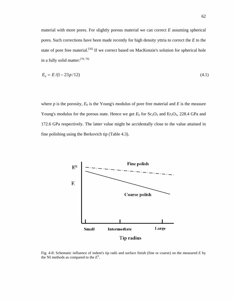
62

material with more pores. For slightly porous material we can correct E assuming spherical

pores. Such corrections have been made recently for high density yttria to correct the E to the

state of pore free material.[56] If we correct based on MacKenzie's solution for spherical hole

in a fully solid matter:[78, 79]

)12/231/(0 pEE −= (4.1)

where p is the porosity, E0 is the Young's modulus of pore free material and E is the measure

Young's modulus for the porous state. Hence we get E0 for Sc2O3 and Er2O3, 228.4 GPa and

172.6 GPa respectively. The latter value might be accidentally close to the value attained in

fine polishing using the Berkovich tip (Table 4.3).

Fig. 4-8: Schematic influence of indent's tip radii and surface finish (fine or coarse) on the measured E by the NI methods as compared to the ES.

63

4.4.4. NI Stress – Strain Curves

An obvious advantage of using spherical indenters is our ability to obtain NI stress – strain

curves. From the results shown in Figs. 4.6 and 4.7, it is reasonable to conclude that:

1. The NI σy values of Sc2O3 and Er2O3 depend on surface roughness. For the finer

polish, σy is higher and the scatter is much smaller.

2. The values of σy at the Edge of the Sc2O3 sample are higher than those in the

center. The reason for this state of affairs is not clear, but may be related to the

fact that the center rim was denser or had a slightly smaller grain size.

3. The NI σy of fully dense Sc2O3, with ≈ 1 µm grains, is ≈ 7 GPa, a value that is

very comparable to the values obtained for Y2O3 using the same technique and

slightly higher than the value in Er2O3 where the grain size is 2.8±0.4 µm.

4.4.5. Fracture Toughness

The K1C obtained herein for Sc2O3 based on the E in the dynamic method, 1.4±0.3 MPam1/2,

or , in the NI method, 1.3±0.3 MPam1/2 are consistent with Gogotsi's value of 1.49±0.03

MPam1/2 [70, 80] for 98.7% dense Sc2O3 attained using single edge notch beams. The similarity

in these results supports to some extent the use of VIF after careful surface treatments.[40] For

Er2O3 the HV in the polycrystalline material measured here, 7.5±0.3 GPa is consistent with

the average results of Er2O3 single crystal measured by Petrovic et al.[66, 67] The K1C based on

the E attained here using the NI method, which is close to ES (Table 4.2), 1.9±0.4 MPam1/2, is

about twice the K1C attained for single crystals.[66, 67]

64

4.5. Summary and Conclusions

E and NI stress – strain curves of fully dense Sc2O3 and slightly porous Er2O3 with a grain

size of ~1-3 µm were determined using a nanoindenter capable of continually measuring the

stiffness, S. Two hemi-spherical indenters with radii of 1.4 µm and 5 µm were used in

addition to a Berkovich tip. We also measured the ES of the same sample. Surface roughness

effect can be clearly seen in the NI stress – strain and S vs. a diagrams. Rough surfaces

increase the scatter of the data specifically in the initial part during which the tip starts

penetrating to the surface. Based on our results we also conclude that both tip sizes and

surface finish have some effect on the E and H determined in these methods and on the

compressive σy values attained using the spherical tips. A smooth surface, with low

roughness, yields less scatter, resulting in clearer diagrams for better analysis. The K1C

attained using the Vickers indentation method after careful treatment of the surface to reveal

the cracks give comparable values for Sc2O3 with literature results and gives twice the K1C for

polycrystalline Er2O3, as compared with the results of Er2O3 single crystal. Based on our

results, we conclude that:

i) Average ESp values of Sc2O3 were calculated to be 211±16 GPa and 180±12 GPa using 1.4

µm and 5 µm tips on roughly polished surfaces, respectively. These values were ~7% and

~21% lower than measured ES value. After fine polishing, ESp values were 217±6 GPa and

208±4 GPa which are ~5% higher and ~9% lower that ES using 1.4 µm and 5 µm tips,

respectively.

ii) ESp values of Er2O3 were calculated to be 158±5 GPa and 153±6 GPa using 1.4 µm and 5 µm

tips on roughly polished surfaces, respectively. These values were ~6% and ~9% lower than

65

measured ES value. After fine polishing, ESp values were 164±3 GPa and 161±5 GPa which

are ~2% higher and ~4% lower that ES using 1.4 µm and 5 µm tips, respectively.

iii) After fine polishing, EBr was calculated to be 215±9 GPa and 172±4 GPa; values that were

~6% lower and ~2% higher than ES for Sc2O3 and Er2O3, respectively. EBr values were lower

and more scattered for roughly polished surfaces.

iv) From the NI stress – strain curves, we estimated the yield point to be 7.3±1 GPa and 9.1±1

GPa for Sc2O3 using 1.4 µm and 5 µm tips after fine polishing, respectively. These values

were lower than the HV (10.8±0.6 GPa) and HBr (12.1±0.5 GPa) values measured on the same

sample. Measured yield point values were lower for rough polishing.

v) We estimated the yield points to be 6±1 GPa and 6.5±0.5 GPa for Er2O3 using 1.4 µm and 5

µm tips after fine polishing, respectively. These values were lower than the HV (7.5±0.3 GPa)

and HBr (9.3±1 GPa) values on the same sample. The yield point values were lower for rough

polishing.

vi) At 1.4±0.3 MPam1/2 average fracture toughness value of Sc2O3 extracted from the Vickers

microhardness indentations were in good agreement with published results on samples with

comparable microstructures. The value of 1.94±0.4 MPam1/2 of Er2O3 was twice of the

attained value of single crystal.

66

Chapter 5 : SURFACE ROUGHNESS – EFECTIVE ZERO POINT - POLISHING QUALITY - TIP SIZE RELATIONSHIPS

5.1. Introduction

The effects of surface roughness and polishing quality on the results obtained for Sc2O3 and

Er2O3 surfaces were discussed in Ch. 4. It is clear that the surface roughness has an influence

on the properties of the materials such as E and σy. The polishing quality is one of the most

important parameters which can affect the surface roughness. In our experiments, our

samples were polished to 1 µm or 0.25 µm. We also observed a tip size effect on the

materials examined. In this chapter, we will go over these effects. We will clarify the tip size

effect by using three more polycrystalline materials which are B4C and MgAl2O4.

5.2. Experimental Details

A CSM attachment enabled nanoindenter was used for NI experiments. The same test

parameters, viz. 45 MHz frequency, 0.05 s-1 strain rate and 2 nm harmonic displacement

target, were selected for all of the tests. Two spherical tips of 1.4 µm radii and 5 µm radii and

a Berkovich tip were used. Generally, 5 to 10 indents were done in different locations at

maximum loads of 50 mN, 80 mN and 500 mN for the 1.4 µm and 5 µm spherical tips and

the Berkovich tip, respectively.

67

ESp of the materials we have used in our experiments were calculated using S vs. a method

which was explained in Ch. 2. ESp calculations for 1.4 µm and 5 µm radii spherical tips were

done up to a = 800 nm and a = 1700 nm of the S vs. a data, respectively. Zero point

corrections were applied to the data before the ESp calculations of all of the experiments and

obtained δ values by the method explained in Ch. 2. [34] NI experiments were completed on

MgAl2O4 and B4C using both tip sizes after polishing with 1 µm size diamond solution in

order to observe the tip size effect on δ and surface roughness relationship. The Y2O3, Er2O3

and Sc2O3 surfaces were indented twice; after polishing with 1 µm and then again with 0.25

µm size diamond solutions. Then the effect of polishing quality on the surface roughness and

δ were investigated.

5.3. Results

5.3.1. Zero point correction , ESp and Rq Values

Calculated effective δ values showed differences depending on polishing quality and tip size.

The highest δ values were observed on Sc2O3 by both spherical tips when the polishing

quality was 1 µm. Y2O3 had the second highest δ value for the 1.4 µm tip. MgAl2O4 showed

the second highest δ value for the 5 µm size tip. After 0.25 µm fine polishing applied to the

samples, δ values decreased significantly for both of the tip sizes.

In the same manner, ESp values demonstrated better agreement with the ES values after fine

polishing. Y2O3 gave 168±3 GPa and 158±3 GPa modulus values before fine polishing by 1.4

µm and 5 µm size tips, respectively. These values are 4.5% and 10.2% lower than the ES.

68

However, the obtained numbers 177±7 GPa and 166±3 GPa after fine polishing render the

results 0.5% and 5.5% closer to the ES values for the 1.4 µm and 5 µm size tips, respectively.

Fine polishing on Sc2O3 increases the proximity from 7% to 4.4% for the 1.4 µm size tip and

from 20.7% to 8.4% for 5 µm size tip.

Surface roughness measurements of Y2O3, Sc2O3 and Er2O3 which were polished by both of

the diamond solutions clearly showed the effect of polishing on Rq. Rq values were reduced

from 14 nm to 9 nm for Y2O3, from 66 nm to 7 nm for Sc2O3 and from 48 nm to 24 nm for

Er2O3.

All of the experiment results are listed in Table 5.1.

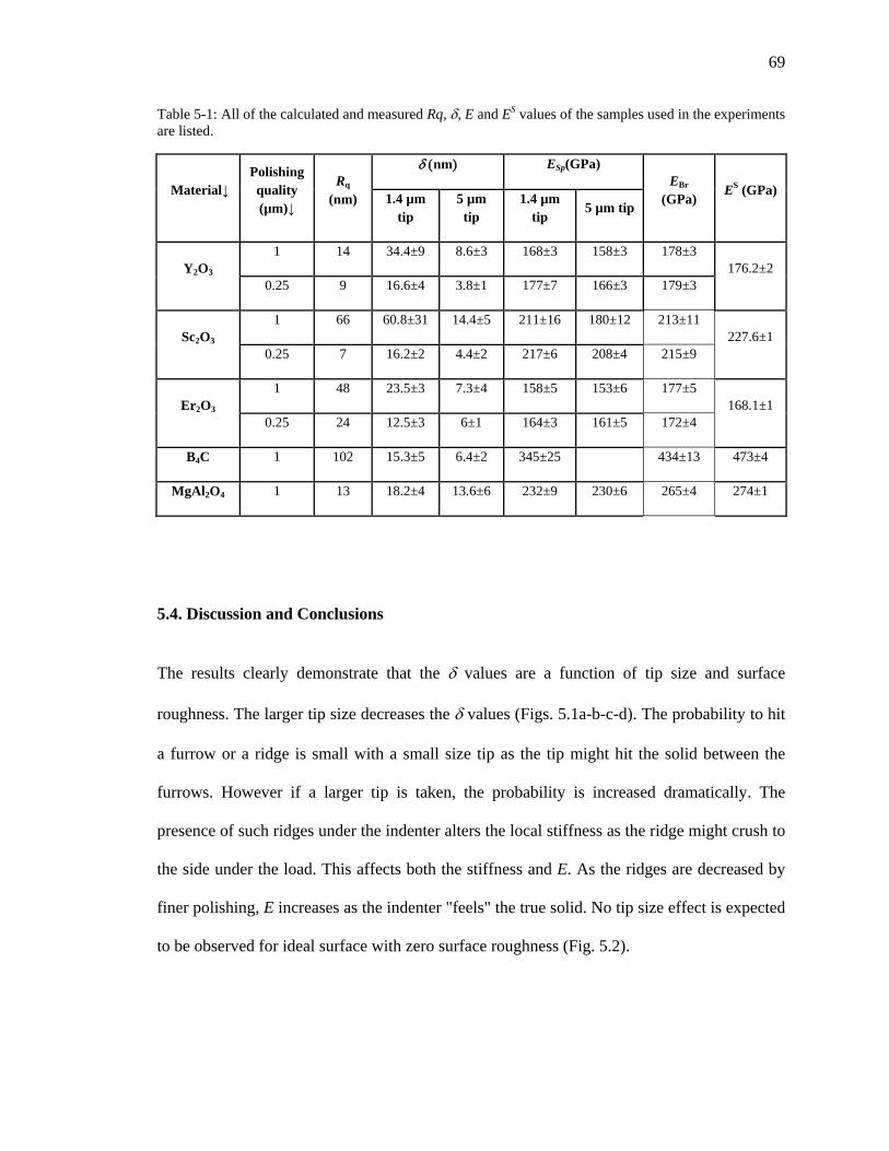
69

Table 5-1: All of the calculated and measured Rq, δ, E and ES values of the samples used in the experiments are listed.

Material↓ Polishing quality (µm)↓

Rq (nm)

δ (nm) ESp(GPa) EBr

(GPa) ES (GPa) 1.4 µm

tip 5 µm tip

1.4 µm tip

5 µm tip

Y2O3 1 14 34.4±9 8.6±3 168±3 158±3 178±3

176.2±2 0.25 9 16.6±4 3.8±1 177±7 166±3 179±3

Sc2O3 1 66 60.8±31 14.4±5 211±16 180±12 213±11

227.6±1 0.25 7 16.2±2 4.4±2 217±6 208±4 215±9

Er2O3 1 48 23.5±3 7.3±4 158±5 153±6 177±5

168.1±1 0.25 24 12.5±3 6±1 164±3 161±5 172±4

B4C 1 102 15.3±5 6.4±2 345±25

434±13 473±4

MgAl2O4 1 13 18.2±4 13.6±6 232±9 230±6 265±4 274±1

5.4. Discussion and Conclusions

The results clearly demonstrate that the δ values are a function of tip size and surface

roughness. The larger tip size decreases the δ values (Figs. 5.1a-b-c-d). The probability to hit

a furrow or a ridge is small with a small size tip as the tip might hit the solid between the

furrows. However if a larger tip is taken, the probability is increased dramatically. The

presence of such ridges under the indenter alters the local stiffness as the ridge might crush to

the side under the load. This affects both the stiffness and E. As the ridges are decreased by

finer polishing, E increases as the indenter "feels" the true solid. No tip size effect is expected

to be observed for ideal surface with zero surface roughness (Fig. 5.2).

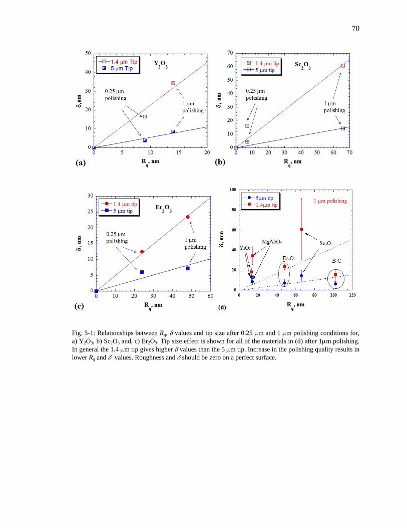
70

Fig. 5-1: Relationships between Rq, δ values and tip size after 0.25 µm and 1 µm polishing conditions for, a) Y2O3, b) Sc2O3 and, c) Er2O3. Tip size effect is shown for all of the materials in (d) after 1µm polishing. In general the 1.4 µm tip gives higher δ values than the 5 µm tip. Increase in the polishing quality results in lower Rq and δ values. Roughness and δ should be zero on a perfect surface.

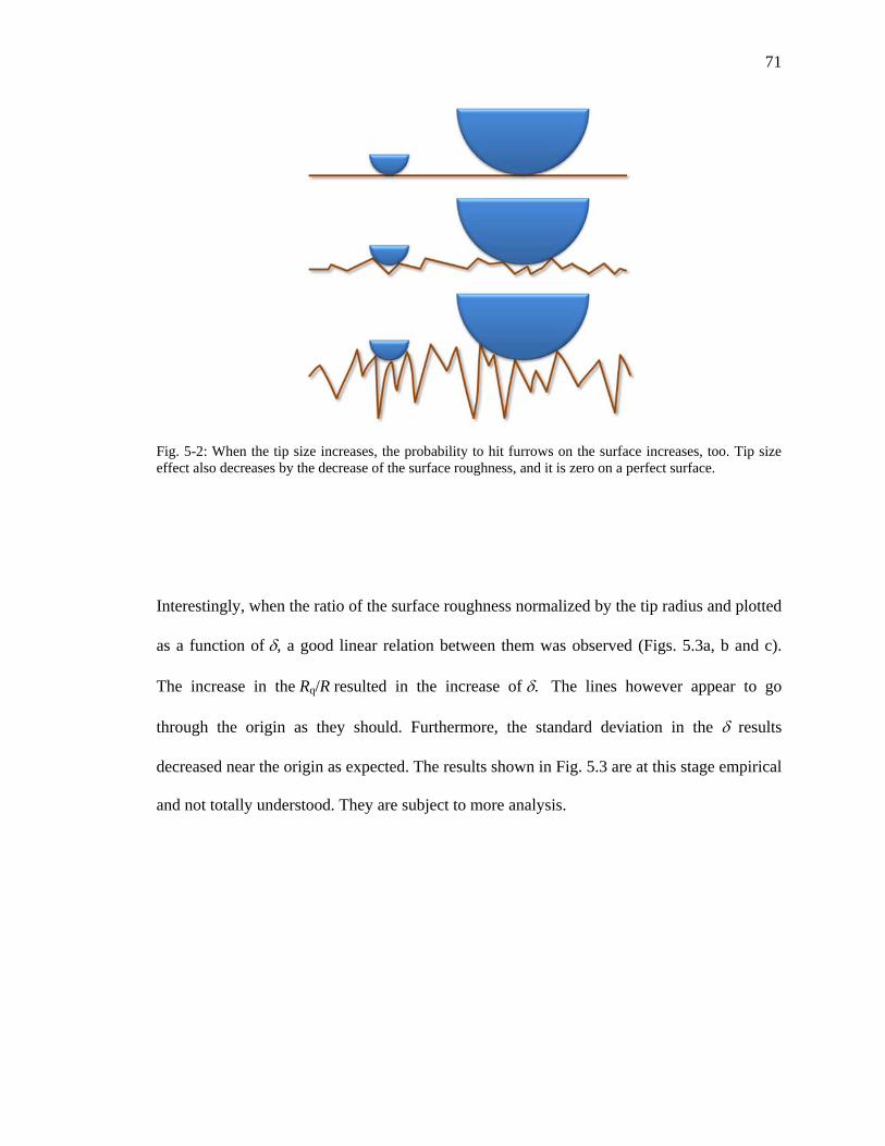
71

Fig. 5-2: When the tip size increases, the probability to hit furrows on the surface increases, too. Tip size effect also decreases by the decrease of the surface roughness, and it is zero on a perfect surface.

Interestingly, when the ratio of the surface roughness normalized by the tip radius and plotted

as a function of δ, a good linear relation between them was observed (Figs. 5.3a, b and c).

The increase in the Rq/R resulted in the increase of δ. The lines however appear to go

through the origin as they should. Furthermore, the standard deviation in the δ results

decreased near the origin as expected. The results shown in Fig. 5.3 are at this stage empirical

and not totally understood. They are subject to more analysis.

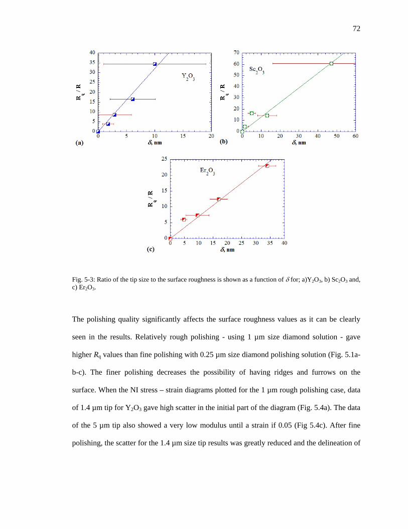
72

Fig. 5-3: Ratio of the tip size to the surface roughness is shown as a function of δ for; a)Y2O3, b) Sc2O3 and, c) Er2O3.

The polishing quality significantly affects the surface roughness values as it can be clearly

seen in the results. Relatively rough polishing - using 1 µm size diamond solution - gave

higher Rq values than fine polishing with 0.25 µm size diamond polishing solution (Fig. 5.1a-

b-c). The finer polishing decreases the possibility of having ridges and furrows on the

surface. When the NI stress – strain diagrams plotted for the 1 µm rough polishing case, data

of 1.4 µm tip for Y2O3 gave high scatter in the initial part of the diagram (Fig. 5.4a). The data

of the 5 µm tip also showed a very low modulus until a strain if 0.05 (Fig 5.4c). After fine

polishing, the scatter for the 1.4 µm size tip results was greatly reduced and the delineation of

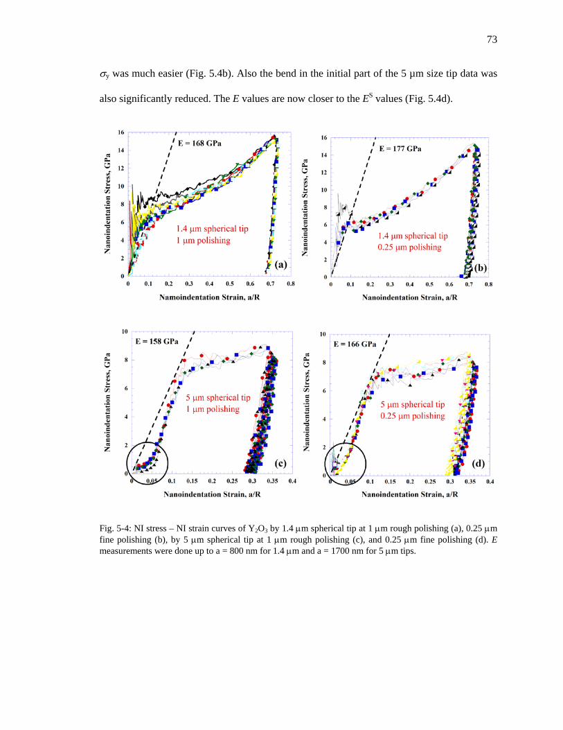
73

σy was much easier (Fig. 5.4b). Also the bend in the initial part of the 5 µm size tip data was

also significantly reduced. The E values are now closer to the ES values (Fig. 5.4d).

Fig. 5-4: NI stress – NI strain curves of Y2O3 by 1.4 µm spherical tip at 1 µm rough polishing (a), 0.25 µm fine polishing (b), by 5 µm spherical tip at 1 µm rough polishing (c), and 0.25 µm fine polishing (d). E measurements were done up to a = 800 nm for 1.4 µm and a = 1700 nm for 5 µm tips.

74

Chapter 6 : SUMMARY and CONCLUSIONS

6.1. Summary and Conclusions

In this thesis, we principally discussed the characterization of hard, brittle polycrystalline

solids using principally NI. We briefly introduced tip types and then focused on spherical tips

which were mainly used in all of our experiments. We explained a method to plot S vs. a

diagrams. Based on this work, it is obvious that the S vs. a plots are a powerful, and relatively

simple, technique to measure the E of polycrystalline ceramics and other hard solids.

A distinct advantage to using spherical NI is the fact that one can also obtain NI stress –

strain curves that can be quite informative about the mechanical properties of the materials as

compared to the commonly used load – displacement diagrams. NI stress – strain curves

enable one to determine the elastic and elastic – plastic regimes.

In Chapter 3 and 4, we reported our work on the polycrystalline binary oxides Y2O3, Sc2O3

and Er2O3. The E and H values were measured by using spherical and sharp indenters. The

Young's moduli of these solids were determined from S vs a curves. We also plotted the NI

stress – strain curves. These results, in turn, were compared with the hardness values

obtained using Berkovich tips. We also measured the Vickers hardness values and compared

to those obtained from the NI stress-strain curves and those obtained from the Berkovich tip.

The influence of polishing quality on surface roughness and the effect of the latter on the

mechanical properties of Sc2O3 and Er2O3 were also examined and reported in Ch. 4. The

75

relationship between the polishing quality – viz. surface roughness – effective zero point and

tip size on the following solids: Y2O3, Sc2O3, Er2O3, B4C, MgAl2O4 and LiTaO3 were

discussed in Ch. 5. Based on our results we concluded that:

• NI is an excellent way to determine the mechanical properties of polycrystalline

ceramics which are brittle solids that cannot be otherwise tested at room temperature.

• The E values calculated using spherical indenters were always smaller than those

measured by the Berkovich indenter. It follows that sharper tips yield higher E

values. The E values of both of all tips, however, were close to those measured by

ultrasound, ES.

• The H values obtained using the Vickers tip are always lower than those obtained

using Berkovich tips. Confirming this notion is the fact that the yield points obtained

from the NI stress – strain curves - a value that can be considered to be the NI

spherical "hardness" - is less than the Vickers hardness.

• A tip size effect is observed. In general, the smaller radii tips resulted in higher E

values than larger ones. The yield points, on the other hand showed quite a bit of

scatter. Within that scatter, no tip size effect was observed. The scatter, however, was

a strong function of surface roughness, with rough surfaces yielding higher scatter.

• The K1C values calculated in this work, except for Er2O3, are in a good agreement

with published results in the literature. Calculated K1C values for Er2O3 are

approximately 50% below its single crystal values in the literature.

• The polishing quality clearly affects the surface roughness of the materials. Finer

polishing decreases the furrows and surface roughness, so the tip can better access the

true surface of the material. More precise material characterization can be made by

this way.

76

• Smoother surfaces result in less scatter and values of E that are closer to those

obtained from ultrasound. The effect of the surface roughness on the NI stress – strain

curves was also investigated. Higher roughness resulted in much more scatter in both

the elastic and plastic regions. We observed a bending in the initial section of the 5

µm radii tip data for the rough polishing. After the fine polishing this bending was

significantly reduced.

6.2. Future Work

Some future work is pointed for better understanding of S vs. a method and NI stress – strain

curves and surface roughness effect;

• Material characterization of thin films can be worked by using S vs. a method and NI

stress – strain diagrams.

• Influence of the surface roughness on the material characterization of thin films is

unknown. This knowledge can be extended. Also, some work on a standard material

such as fused silica can be done. It can be polished by 0.05 µm, 0.25 µm and 1 µm

polishing solutions, and then it can be tested for surface roughness with various

spherical tips; 1.4 µm, 5 µm and even 21 µm.

• We only use effective zero point determination method on bulk materials and only

by spherical tips. We don’t know how accurate this method can be on thin films.

Whether the method can be also extended to other tip types needs to be explored.

• The effect of tilted surfaces on the characterization and also its influence on the

effective zero point determination should be observed.

77

• The effect of ceramic hardness on the NI should be further checked in order to

understand why the elastic modulus measured by NI is low as compared with the

dynamic elastic modulus.

78

LIST OF REFERENCES

1. Tabor, D., Hardness of Metals. 1951, Clarendon, U.K.: Oxford.

2. Oliver, W.C. and G.M. Pharr, An improved technique for determining hardness and elastic-modulus using load and displacement sensing indentation experiments. Journal of Materials Research, 1992. 7(6): p. 1564-1583.

3. Oliver, W.C. and G.M. Pharr, Measurement of hardness and elastic modulus by instrumented indentation: Advances in understanding and refinements to methodology. Journal of Materials Research, 2004. 19(1): p. 3-20.

4. Field, J.S. and M.V. Swain, Determining the mechanical properties of small volumes of material from submicrometer spherical indentations. Journal of Materials Research, 1995. 10(1): p. 101-112.

5. Field, J.S. and M.V. Swain, A simple predictive model for spherical indentation. Journal of Materials Research, 1992. 8(2): p. 297-306.

6. Quinn, G.D., et al., Fracture toughness of advanced ceramics at room temperature. Journal of Research of the National Institute of Standards and Technology, 1992. 97(5): p. 579-607.

7. Anstis, G.R., et al., A critical evaluation of indentation techniques for measuring fracture toughness: I, direct crack measurements. Journal of the American Ceramic Society, 1981. 64(9): p. 533-538.

8. Niihara, K., R. Morena, and D.P.H. Hasselman, Evaluation of KIC of brittle solids by the indentation method with a low crack-to-indent ratios. Journal of Materials Science Letters, 1982. 1(1): p. 13-16.

9. A.G. Evans and E.A. Charles, Fracture toughness determination by indentation. J. American Ceramic Society, 1976. 59: p. 371-372.

10. Laugier, M.T., The elastic/plastic indentation of ceramics. Journal of Materials Science Letters, 1985. 4(12): p. 1539-1541.

11. Lankford, J., Indentation microstructure in Palmqvist crack regime: implications for fracture toughness evaluation by the indentation method. Journal of Materials Science Letters, 1982. 1(11): p. 493-495.

12. Brinell, J.A., in II. Cong. Int. Methodes d'Essai. 1900: Paris.

13. Herbert, E.G., et al., On the measurement of stress-strain curves by spherical indentation. Thin Solid Films, 2001. 398: p. 331-335.

79

14. Basu, S., A. Moseson, and M.W. Barsoum, On the determination of spherical nanoindentation stress-strain curves. Journal of Materials Research, 2006. 21: p. 2628-2637.

15. Doerner, M. and W. Nix, A method for interpreting the data from depth-sensing indentation instruments. J. Mater. Res, 1986. 1(4): p. 601-609.

16. Swain, M.V., Mechanical property characterisation of small volumes of brittle materials with spherical tipped indenters. Materials Science and Engineering a-Structural Materials Properties Microstructure and Processing, 1998. 253(1-2): p. 160-166.

17. Swain, M.V. and J.T. Hagan, Indentation plasticity and the ensuing fracture of glass. Journal of Physics D: Applied Physics, 1976. 9(15): p. 2201-2214.

18. Field, J.S. and M.V. Swain, The indentation characterisation of the mechanical properties of various carbon materials: Glassy carbon, coke and pyrolytic graphite. Carbon, 1996. 34(11): p. 1357-1366.

19. Li, X.D. and B. Bhushan, A review of nanoindentation continuous stiffness measurement technique and its applications. Materials Characterization, 2002. 48(1): p. 11-36.

20. Lawn, B.R., Indentation of ceramics with spheres: A century after Hertz. Journal of the American Ceramic Society, 1998. 81(8): p. 1977-1994.

21. Bushby, A.J., Nano-indentation using spherical indenters. Nondestructive Testing and Evaluation, 2001. 17(4): p. 213 - 234.

22. Basu, S., On Spherical Nanoindentation Stress-Strain Curves, Creep and Kinking Nonlinear Elasticity in Brittle Hexagonal Single Crystals, in Materials Science and Engineering. 2008, Drexel University: Philadelphia.

23. Fischer-Cripps, A.C., A review of analysis methods for sub-micron indentation testing. Vacuum, 2000. 58(4): p. 569-585.

24. Bobji, M.S., S.K. Biswas, and J.B. Pethica, Effect of roughness on the measurement of nanohardness - a computer simulation study. Applied Physics Letters, 1997. 71(8): p. 1059-1061.

25. Shibutani, Y. and A. Koyama, Surface roughness effects on the displacement bursts observed in nanoindentation. Journal of Materials Research, 2004. 19(1): p. 183-188.

26. Kim, J.Y., et al., Surface roughness effect in instrumented indentation: A simple contact depth model and its verification. Journal of Materials Research, 2006. 21(12): p. 2975-2978.

27. Jiang, W.G., J.J. Su, and X.Q. Feng, Effect of surface roughness on nanoindentation test of thin films. Engineering Fracture Mechanics, 2008. 75(17): p. 4965-4972.

80

28. Kim, J.Y., et al., Influence of surface-roughness on indentation size effect. Acta Materialia, 2007. 55(10): p. 3555-3562.

29. Walter, C., et al. Finite element simulation of the effect of surface roughness on nanoindentation of thin films with spherical indenters. 2007: Elsevier Science Sa.

30. Walter, C. and C. Mitterer, 3D versus 2D finite element simulation of the effect of surface roughness on nanoindentation of hard coatings. Surface & Coatings Technology, 2009. 203(20-21): p. 3286-3290.

31. Johnson, K.L., Indentation Contact Mechanics. 1985, Cambridge: Cambridge University Press.

32. Hertz, H., Miscellaneous papers. London: Jones & Schott. 1863, Macmillan.

33. Sneddon, I.N., The relation between load and penetration in the axisymmetric boussinesq problem for a punch of arbitrary profile. International Journal of Engineering Science, 1965. 3(1): p. 47-57.

34. Moseson, A.J., S. Basu, and M.W. Barsoum, Determination of the effective zero point of contact for spherical nanoindentation. Journal of Materials Research, 2008. 23(1): p. 204-209.

35. Fischer-Cripps, A.C., Critical review of analysis and interpretation of nanoindentation test data. Surface & Coatings Technology, 2006. 200(14-15): p. 4153-4165.

36. Moseson, A.J., Spherical Nanoindentation: Insights And Improvements, Including Stress-Strain Curves and Effective Zero Point Determination, in Materials Science and Engneering. 2007, Drexel University: Philadelphia.

37. Lawn, B.R., A.G. Evans, and D.B. Marshall, Elastic/plastic indentation damage in ceramics: the median/radial crack system. Journal of the American Ceramic Society, 1980. 63(9-10): p. 574-581.

38. Smith, S.S., P. Magnusen, and B.J. Pletka, Fracture toughness od glass using the indentation fracture technique, in 3rd International Symposium On Fracture Mechanics of Ceramics. 1981. p. 33-45.

39. Desmaisonbrut, M., et al., Influence of processing conditions on the microstructure and mechanical properties of sintered yttrium oxide. Journal of the American Ceramic Society, 1995. 78(3): p. 716-722.

40. Greenberg, Y., M. Aizenshtein, and O. Yeheskel, The hardness and fracture toughness of transparent yttria, in NRCN. 1996: Israel.

41. MetroPro Surface Texture Parameters Manual, Zygo, Editor. 2005.

42. Yeheskel, O. and O. Tevet, Elastic moduli of transparent yttria. Journal of the American Ceramic Society, 1999. 82(1): p. 136-144.

81

43. Wei, G.C., et al., Lanthana-atrengthened yttria domes and windows. SPIE, 1988. 968: p. 5-13.

44. Greskovich, C.D. and C.R. O'Clair, Yttrium Oxide Ceramic Body, U.S. Patent, Editor. 1988, General Electric Company: United States.

45. Hartnett, T., M. Greenberg, and R.L. Gentilmen, Optically Transparent Yttrium Oxide, U.S. Patent, Editor. 1988, Raytheon Company: United States.

46. Rhodes, W.H., Controlled transient solid second-phase sintering of yttria. Journal of the American Ceramic Society, 1981. 64(1): p. 13-19.

47. Mouzon, J., Synthesis of Yb:Y2O3 nanoparticles and fabrication of transparent polycrystalline yttria ceramics. 2005, Luleå University of Technology: Sweden.

48. Mouzon, J., et al., Effect of drying and dewatering on yttria precursors with transient morphology. Journal of the American Ceramic Society, 2006. 89(10): p. 3094-3100.

49. Dutta, S.K. and G.A. Gazzara, Method for production of transparent yttrium oxide, U.S. Patent, Editor. 1975, United States of America as represented by the Secretary of Army: United States.

50. Kumar, A.S., A.R. Durai, and T. Sornakumar, Yttria ceramics: cutting tool application. Materials Letters, 2004. 58(11): p. 1808-1810.

51. Gogotsi, G.A., Thermal stress behaviour of yttria, scandia and AIN ceramics. Ceramurgia International, 1980. 6(1): p. 31-35.

52. Barzilai, S., et al., Interface phenomena in the Y2O3/(Al-Cu) system. Materials Science and Engineering a-Structural Materials Properties Microstructure and Processing, 2006. 420(1-2): p. 291-295.

53. Cao, X.Q., Application of rare earths in thermal barrier coating materials. Journal of Materials Science & Technology, 2007. 23(1): p. 15.

54. Unal, O. and M. Akinc, Compressive properties of yttrium oxide. Journal of the American Ceramic Society, 1996. 79(3): p. 805-808.

55. Tani, T., et al., Grain size dependences of vickers microhardness and fracture toughness in Al2O3 and Y2O3 ceramics. Ceramics International, 1986. 12(1): p. 33-37.

56. Yeheskel, O., et al., Effect of Initial Particle and Agglomerate Size on the Elastic Moduli of Porous Yttria (Y2O3). Journal of the American Ceramic Society, 2009. 92(8): p. 1655-1662.

57. Basu, S. and M.W. Barsoum, Deformation micromechanisms of ZnO single crystals as determined from spherical nanoindentation stress-strain curves. Journal of Materials Research, 2007. 22: p. 2470-2477.

82

58. Basu, S., M.W. Barsoum, and S.R. Kalidindi, Sapphire: A kinking nonlinear elastic solid. Journal of Applied Physics, 2006. 99(6).

59. Basu, S., et al., Spherical nanoindentation and deformation mechanisms in freestanding GaN films. Journal of Applied Physics, 2007. 101(8).

60. Basu, S., A.G. Zhou, and M.W. Barsoum, Reversible dislocation motion under contact loading in LiNbO3 single crystal. Journal of Materials Research, 2008. 23(5): p. 1334-1338.

61. Basu, S., A. Zhou, and M.W. Barsoum, On spherical nanoindentations, kinking nonlinear elasticity of mica single crystals and their geological implications. Journal of Structural Geology, 2009. 31(8): p. 791-801.

62. Palko, J.W., et al., Elastic constants of yttria (Y2O3) monocrystals to high temperatures. Journal of Applied Physics, 2001. 89(12): p. 7791-7796.

63. Lu, J., et al., Yb3+:Sc2O3 ceramic laser. Applied Physics Letters, 2003. 83(6): p. 1101-1103.

64. Tokurakawa, M., et al., Diode-pumped sub-100 fs Kerr-lens mode-locked Yb3+: Sc2O3 ceramic laser. Optics Letters, 2007. 32(23): p. 3382-3384.

65. Li, J.G., T. Ikegami, and T. Mori, Fabrication of transparent, sintered Sc2O3 ceramics. Journal of the American Ceramic Society, 2005. 88(4): p. 817-821.

66. Petrovic, J.J., et al., Synthesis and properties of erbium oxide single crystals. Ceram Eng. Sci. Proc., 1999. 20: p. 3-10.

67. Petrovic, J.J., et al., Mechanical behavior of erbium oxide single crystals, in 24th Annual Cocoa Beach Conference. 2000, Journal of American Ceramic Society: Cocoa Beach, Florida.

68. Dole, S., D. Hunter Jr, and F. Calderwood, Elastic properties of polycrystalline scandium and thulium sesquioxides. Journal of the American Ceramic Society, 1977. 60(3): p. 167-68.

69. Sharif, A.A., et al., Elastic constants of erbia single crystals. Journal of the American Ceramic Society, 2000. 83(9): p. 2246-2250.

70. Gogotsi, G., S. Mudrik, and V. Galenko, Evaluation of fracture resistance of ceramics: Edge fracture tests. Ceramics International, 2007. 33(3): p. 315-320.

71. Makino, Y. and S. Miyake, Estimation of bulk moduli of compounds by empirical relations between bulk modulus and interatomic distance. Journal of Alloys and Compounds, 2000. 313(1-2): p. 235-241.

72. Yusa, H., et al., High-Pressure Phase Transition to the Gd2S3 Structure in Sc2O3: A New Trend in Dense Structures in Sesquioxides. Inorganic Chemistry, 2009. 48(16): p. 7537-7543.

83

73. Barzilai, S., I. Halevy, and O. Yeheskel, The Bulk Modulus of Sc2O3: ab-initio Calculations and Experimental Results. 2009.

74. Manning, W.R., O.H. Jr., and B.R.P. Jr., Elastic Properties of Polycrystalline Yttrium Oxide, Dysprosium Oxide, Holmium Oxide, and Erbium Oxide: Room Temperature Measurements. Journal of the American Ceramic Society, 1969. 52(8): p. 436-442.

75. The International Centre for Diffraction Data, I.C.D.D., Sc2O3, card # 43-1028, Er2O3, card # 43-1007

76. Timoshenko, S. and J. Goodier, Theory of elasticity. 3rd ed. 1970, New York: McGraw-Hill.

77. Kang, S.K., et al., Effective indenter radius and frame compliance in instrumented indentation testing using a spherical indenter. Journal of Materials Research, 2009. 24(9): p. 2965-2973.

78. Pal, R., Porosity-dependence of effective mechanical properties of pore-solid composite materials. Journal of Composite Materials, 2005. 39(13): p. 1147-1158.

79. Mackenzie, J.K., The Elastic Constants of a Solid containing Spherical Holes. Proceedings of the Physical Society. Section B, 1950. 63(1): p. 2-11.

80. Gogotsi, G., Fracture resistance of ceramics: direct measurements. Advances in Science and Technology, 2006. 45: p. 95–100.

84