Mechanical simulation of a single sheet of graphene: a study on

the aplications of nanomaterials

Ricardo Silva Rosa Pedrosaricardopedrosa@ist.utl.pt

Instituto Superior Tecnico, Lisboa, Portugal

May 2016

Abstract

Graphene is a bidimensional carbon allotrope with a hexagonal molecular lattice, in which itsmechanical, electrical and optical properties have motivated an intense level of research of the scientificcommunity in the last decade. This dissertation’s main objectives are the development of a consistentfinite element model for the both linear and non linear simulation of graphene’s mechanical behaviour.Two interatomic potentials were used in the linear simulations of the model to assess their influenceon the elastic properties. Non linear simulations were performed to obtain graphene’s mechanicalstrength. The finite element model results are compared with results collected from previous works onthe fields of molecular dynamics and other atomistic computational methods. The present study showsthat finite element models are able to predict well the mechanical properties of graphene.Keywords:Graphene, Nanomaterials, Mechanical Properties, Interatomic Potential, Finite ElementMethod

1. Introduction

Nanostructured materials have attracted a con-siderable amount of interest and research in thelast few years due to their remarkable mechani-cal [10], electrical [24], and optical properties. Inparticular, graphene has been intensely studied,due its many applications. Some of the more ap-plications are: structural composites like ceramicgraphene-ceramic ones that improve brittle fracturebehaviour of the ceramics used in jet engines with-out compromising heat resistance [20], metal andpolymer nanocomposites that are stiffer, strongerand lighter than most of the composites availabletoday [? ]; in electronics, graphene and CNTshave been researched for future transistors that maygreatly increase information processing speed [7];graphene is expected to improve hydrogen storagecapabilities, and even efficient electrical power stor-age in the form of supercapacitors [21].

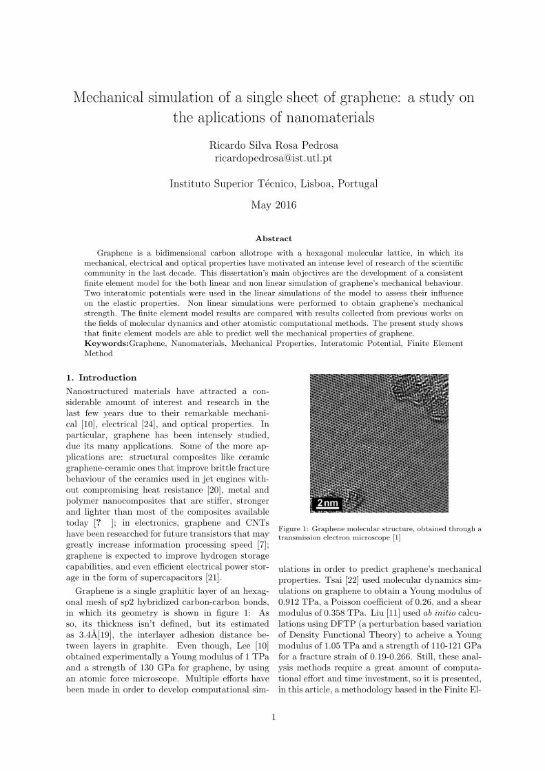
Graphene is a single graphitic layer of an hexag-onal mesh of sp2 hybridized carbon-carbon bonds,in which its geometry is shown in figure 1: Asso, its thickness isn’t defined, but its estimatedas 3.4A[19], the interlayer adhesion distance be-tween layers in graphite. Even though, Lee [10]obtained experimentally a Young modulus of 1 TPaand a strength of 130 GPa for graphene, by usingan atomic force microscope. Multiple efforts havebeen made in order to develop computational sim-

Figure 1: Graphene molecular structure, obtained through atransmission electron microscope [1]

ulations in order to predict graphene’s mechanicalproperties. Tsai [22] used molecular dynamics sim-ulations on graphene to obtain a Young modulus of0.912 TPa, a Poisson coefficient of 0.26, and a shearmodulus of 0.358 TPa. Liu [11] used ab initio calcu-lations using DFTP (a perturbation based variationof Density Functional Theory) to acheive a Youngmodulus of 1.05 TPa and a strength of 110-121 GPafor a fracture strain of 0.19-0.266. Still, these anal-ysis methods require a great amount of computa-tional effort and time investment, so it is presented,in this article, a methodology based in the Finite El-

1

ement Method (FEM), available and widely used inengineering aplications, to study with precision andquickness the mechanical properties (linear elasticand non linear) of graphene. Some authors have al-ready used this method (originally devised by Ode-gard [17] with sucess: Meo and Rossi [12] used nonlinear springs to modulate the carbon links in CNTsand graphene, and obtained, for the last, a Youngmodulus of 0.945 GPa.

2. Background2.1. Molecular mechanics

An important component in molecular mechanicscalculations is the description of the forces betweenindividual atoms. This description is characterizedby a force field. In the most general form, the totalinter-atomic potential energy in a molecule, Utotal,for a nano-structured material is described by thesum of many individual energy contributions re-lated to the interactions between linked atoms, andnon linked atoms, in the molecular lattice, as shownin the equation 1:

Utotal =∑

Ur+∑

Uθ+∑

Uϕ+∑

Uω+∑

Uvw

(1)in which the first four terms represent the inter-actions between bonded atoms and the fifth term,Uvw represents the van der Waals interaction be-tween any non bonded atoms, often described bythe Lennard-Jones potential [3], but here is despiseddue to its weak influence on the mechanical prop-erties of graphene. The electrostatic term of thepotential is also despised. The first four terms de-scribe the atoms motion and position lattice. Ur

is related to the axial deformation on the molecularlink, Uθ is the ’bending’ term and it describes angu-lar motion between three atoms and finally, Uϕ andUω are the in-plane and out-of-plane torsion terms.These interactions are easily interpreted from a ba-sic molecule scheme depicted in figure 2:

Figure 2: Geometry of a simple molecule chain where r23is the interatomic distance, θ234 is the ’bending’ angle andϕ1234 the in-plane torsion angle [3]

Obtaining accurate parameters for a force field

amounts to fitting a set of experimental or empiricaldata to the assumed functional form, specifically,the force constants and equilibrium structure of themolecule. In this article the AMBER [5] and Morse[15] interatomic potentials are used. They are bothrepresented in their harmonized form in equation 2:

Ur =1

2kr(δr)

2 , (2a)

Uθ =1

2kθ(δθ)

2 , (2b)

Uτ = Uϕ + Uω =1

2kτ (δϕ)

2 . (2c)

where kr is the bond stretching force constant, kθis the bond bending force constant and kτ is theequivalent bond torsion term, and δr, δθ and δϕ arethe bond stretching increment, bond angle variationand angle variation of bond twisting, respectively.

2.2. Equivalent beam model

In order to determine the elastic moduli of the beamelements that will compose graphene’s structure, re-lations between the sectional stiffness parameters instructural mechanics and the force-field constantsin molecular mechanics need to be obtained. Forsimplicity reasons, the sections of the bonds areassumed to be identical and circular. The elas-tic properties that need to be obtained are Youngsmodulus E, Poisson’s ratio ν and the shear modu-lus G. The deformation of a space-frame results inchanges of strain energies. Thus, the elastic mod-uli can be determined through the equivalence ofthe energies due to the interatomic interactions pre-sented in equation 2 and the elastic energy that re-sults from the deformation of the space-frame struc-tural elements. As each of the energy terms of equa-tions 2 represents deformations in specific degrees offreedom, the strain energies of structural elementsunder the same deformations in equivalent degreesof freedom will be considered. According to theEuler-Bernoulli beam model from classical struc-tural mechanics, the strain energy UA of a uniformbeam of length L and cross-section A under pureaxial force N is:

UA =1

2

∫ L

0

N2

EAdx =

1

2

EA

L(δL)2 (3)

The strain energy UM of a uniform beam with amoment of inertia I, under pure bending momentM is:

UM =1

2

∫ L

0

M2

EIdx =

1

2

EI

L(2α)2 . (4)

where α denotes the rotational angle at the ends ofthe beam.The strain energy UT of a uniform beam

2

under pure torsion T is:

UT =1

2

∫ L

0

T 2

GJdx =

1

2

GJ

L(δβ)2 . (5)

where δβ is the relative rotation between the endsof the beam and J the polar moment of inertia.The equivalence of bond stretch equation 2a and

axial beam equation 3, bond and beam bendingequations 2b, 4 and bond and beam torsion equa-tions 2c, 5 serves as foundation of the equivalentatomic-beam model that is used in the analysisof graphene’s linear mechanical behaviour. Thisequivalence is presented in a more compact in thefollowing equations:

EA

L= kr,

EI

L= kθ,

GJ

L= kτ . (6)

The thickness of a single sheet of graphene is notwell defined, but for calculation purposes it hasbeen estimated as 3.4 A. As the length of the samecarbon bond is estimated as 1.42 A, the beam el-ement that models this covalent bond will have ashort aspect ratio, and therefore, the Timoshenkoshear correction [18] can be introduced in the clas-sical beam model of equation 4. This correctionchanges the bending energy equation to the form:

UTimoshenko =1

2

EI

L

4 + Φ

1 + Φ(2α)2 . (7)

where Φ is the shear tension coefficient, representedby:given by the expression:

Φ =12EI

GAsL2. (8)

where As = A/Fs, e Fs is the shear correction fac-tor, which takes the following form for a circularsection:

Fs =6 + 12ν + 6ν2

7 + 12ν + 4ν2(9)

The system of equations 6 establish the founda-tion for the application of the theory of structuralmechanics in modeling of graphene or other simi-lar fullerene structures, for linear elastic simulation.For the non linear behaviour a more direct approachbased on the Morse potential is used. This poten-tial is described approximately by the force field ofthe equation:

F = 2βDe(1− exp−βϵr) exp−βϵr . (10)

where β = 2.625A−1 is a constant that controls the’width’ of the potential, De = 6.03105nNA is thedissociation energy and r is the length of the cova-lent bond taken as 1.42 A. In order to get the nonlinear stress-strain curve for the C-C bond, equa-tion 10 is divided by the section area of the carbonbond, which is not well defined because of the ill de-fined thickness of graphene, so therefore the sectionarea is taken as unitary for the non linear studies.

3. Methodology

In this section the finite element model develop-ment methodology is described. In the first sub-section the model’s geometry, material models andelement type are depicted. In the second subsec-tion, the analysis with each own boundary condi-tions are defined for linear elastic simulations. Inthe third subsection, the non linear analysis are de-fined, along with the modifications to the modelthat were needed to study this behaviour.

3.1. Reference model

A finite element model was built in the FEM soft-ware ABAQUS/CAE R⃝. As both linear and nonlinear simulations run on the same geometry, themodel used for the linear elastic simulations ishereby defined as the Reference model, and ev-ery definition made in this subsection is relative tothe reference model. In the following subsection,some modifications are made based on the referencemodel as a starting point.

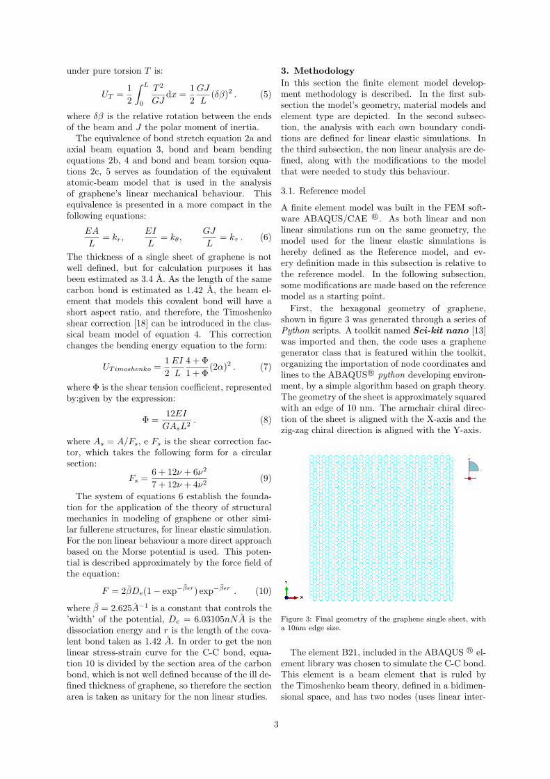
First, the hexagonal geometry of graphene,shown in figure 3 was generated through a series ofPython scripts. A toolkit named Sci-kit nano [13]was imported and then, the code uses a graphenegenerator class that is featured within the toolkit,organizing the importation of node coordinates andlines to the ABAQUS R⃝ python developing environ-ment, by a simple algorithm based on graph theory.The geometry of the sheet is approximately squaredwith an edge of 10 nm. The armchair chiral direc-tion of the sheet is aligned with the X-axis and thezig-zag chiral direction is aligned with the Y-axis.

Figure 3: Final geometry of the graphene single sheet, witha 10nm edge size.

The element B21, included in the ABAQUS R⃝ el-ement library was chosen to simulate the C-C bond.This element is a beam element that is ruled bythe Timoshenko beam theory, defined in a bidimen-sional space, and has two nodes (uses linear inter-

3

polation) that have 6 degrees of freedom: 3 transla-tional and 3 rotational, in every cartesian direction.Regarding the material model, there will be four

material models to be tested within the same frame-work of analysis. Two of the material models willbe based on the Euler-Bernoulli beam approach ofequation 6, one using AMBER force field and theother using the linearized Morse force field. Theother two are developed using AMBER and Morseforce fields, but now with the Timoshenko correc-tion. The material model inputs (Young moduliand shear moduli, the Poisson coefficient of the C-C bond is taken as 0) are expressed in table 1 ,with the four beam model/potential combinationsthat were implemented on the software. The ele-ment section as taken as circular.

Table 1: Force field constants k derived from both inter-atomic potentials used and the results from equation 6 forE, G and section diamater

Interatomic force fields

Data AMBER MORSE

kr

[nN

A

]65.20 84.70

kθ

[nNArad2

]8.76 9.00

kτ

[nNArad2

]2.78 2.78

Timoshenko beam

E[nN

A2

]167.132 292.992

G[nN

A2

]80.828 147.191

d[A]

0.834 0.723

Euler-Bernoulli beam

E[nN

A2

]54.836 90.075

G[nN

A2

]8.70122221 13.912

d[A]

1.466 1.304

These four material models, with its respectivesection geometry, are now defined, so it is nowpossible to present the four simulations that weremade in order to simulate the elastic behaviourof graphene for small deformations. Each simu-lation was tested with each combination of beammodel/potential so a total of 16 simulations wereconducted. The four simulations are:

• Uniaxial traction test in the armchair direction(Ox axis), in order to obtain Ex and νx.

• Uniaxial traction test in the zig-zag direction(Oy axis), in order to obtain Ey and νy.

• Biaxial traction test (XY plane), in order to

obtain the bulk moduli K (in this case an areamoduli) .

• Shear test (XY plane), in order to obtain theshear moduli G.

For the uniaxial tests, one edge was simply su-ported, constraining only the translational degreeof freedom in the direction of the test, while onthe other edge was applied a unitary displacementof 1 A. On the biaxial test the center point of thesheet was constrained in every degree of freedomand the same unitary displacement was applied toevery edge. Relative to the shear test, the centerpoint was also constrained, and in every edge wasapplied a shear load, parallel to the edge direction,in order to apply two cancelling moments.

3.2. Non linear model

Regarding the non linear model, some modificationswere made to the reference model, concerning thestudy of graphene non linear behaviour in order toobtain the mechanical strength of this nanomate-rial. The geometry of this model wasn’t modifiedbecause it is the same material, therefore the samemolecular geometry. To describe the mechanicalbehaviour of the C-C bond, the equivalent atomic-beam method is still used but the equivalence be-tween structural and molecular mechanics is madedirectly thought the Morse potential in its non har-monized form of equation 10, as detailed in theprevious section. This equation only expresses thestretching interaction, as in this section, the remain-ing interactions are despised.

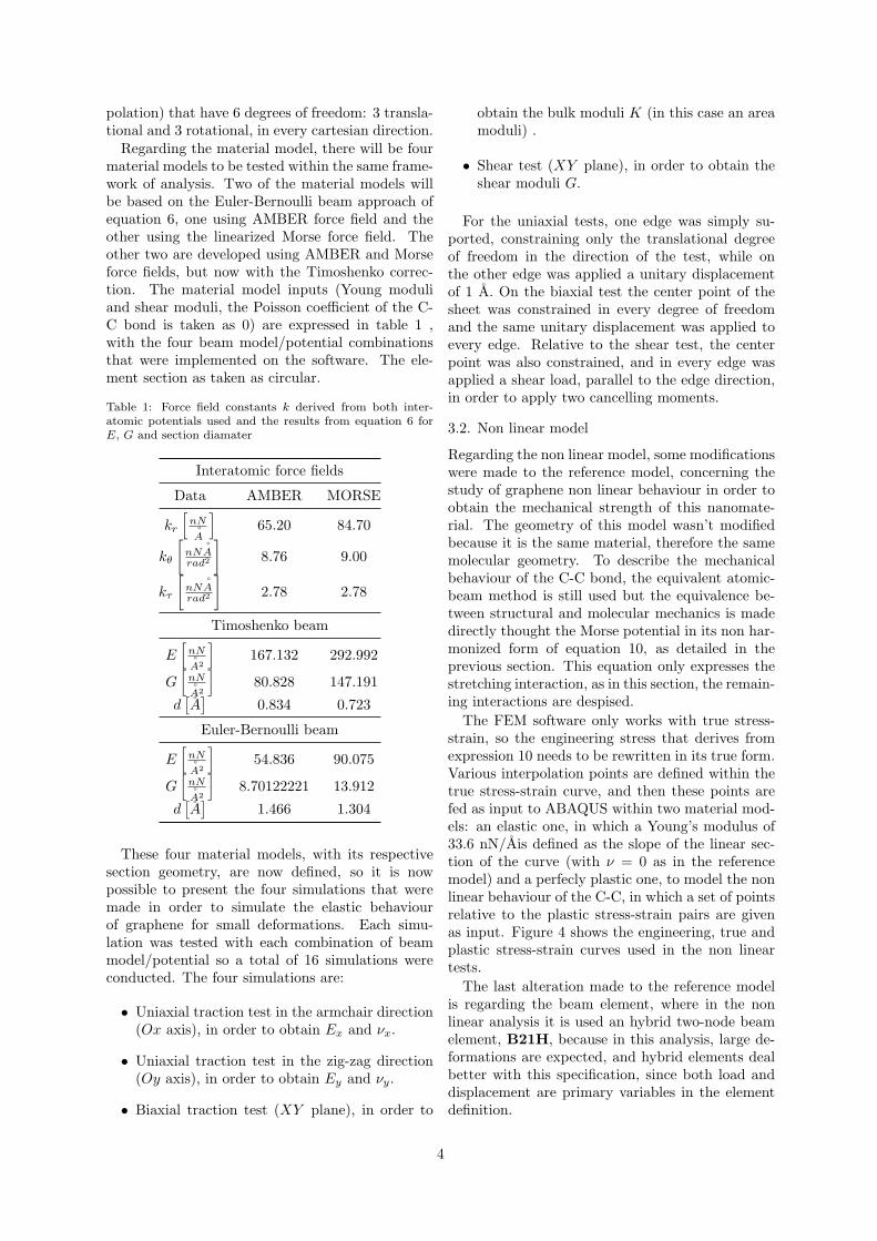
The FEM software only works with true stress-strain, so the engineering stress that derives fromexpression 10 needs to be rewritten in its true form.Various interpolation points are defined within thetrue stress-strain curve, and then these points arefed as input to ABAQUS within two material mod-els: an elastic one, in which a Young’s modulus of33.6 nN/Ais defined as the slope of the linear sec-tion of the curve (with ν = 0 as in the referencemodel) and a perfecly plastic one, to model the nonlinear behaviour of the C-C, in which a set of pointsrelative to the plastic stress-strain pairs are givenas input. Figure 4 shows the engineering, true andplastic stress-strain curves used in the non lineartests.

The last alteration made to the reference modelis regarding the beam element, where in the nonlinear analysis it is used an hybrid two-node beamelement, B21H, because in this analysis, large de-formations are expected, and hybrid elements dealbetter with this specification, since both load anddisplacement are primary variables in the elementdefinition.

4

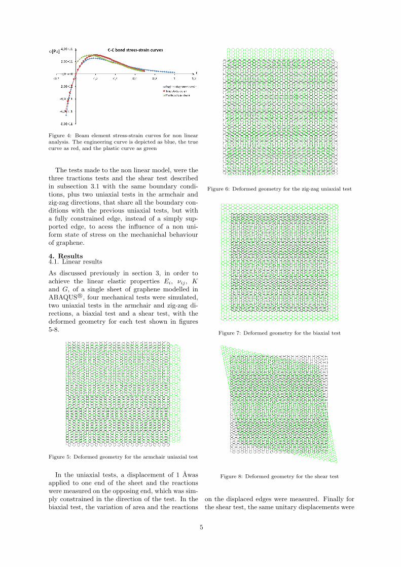
Figure 4: Beam element stress-strain curves for non linearanalysis. The engineering curve is depicted as blue, the truecurve as red, and the plastic curve as green

The tests made to the non linear model, were thethree tractions tests and the shear test describedin subsection 3.1 with the same boundary condi-tions, plus two uniaxial tests in the armchair andzig-zag directions, that share all the boundary con-ditions with the previous uniaxial tests, but witha fully constrained edge, instead of a simply sup-ported edge, to acess the influence of a non uni-form state of stress on the mechanichal behaviourof graphene.

4. Results4.1. Linear results

As discussed previously in section 3, in order toachieve the linear elastic properties Ei, νij , Kand G, of a single sheet of graphene modelled inABAQUS R⃝, four mechanical tests were simulated,two uniaxial tests in the armchair and zig-zag di-rections, a biaxial test and a shear test, with thedeformed geometry for each test shown in figures5-8.

Figure 5: Deformed geometry for the armchair uniaxial test

In the uniaxial tests, a displacement of 1 Awasapplied to one end of the sheet and the reactionswere measured on the opposing end, which was sim-ply constrained in the direction of the test. In thebiaxial test, the variation of area and the reactions

Figure 6: Deformed geometry for the zig-zag uniaxial test

Figure 7: Deformed geometry for the biaxial test

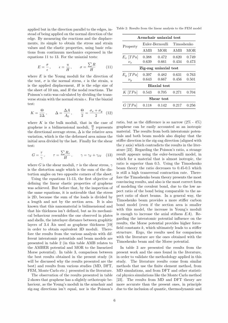
Figure 8: Deformed geometry for the shear test

on the displaced edges were measured. Finally forthe shear test, the same unitary displacements were

5

applied but in the direction parallel to the edges, in-stead of being applied on the normal direction of theedge. By measuring the reactions and the displace-ments, its simple to obtain the stress and strainvalues and the elastic properties, using basic rela-tions from continuum mechanics expressed in theequations 11 to 13. For the uniaxial tests:

E =σ

ϵ, ϵ =

u

H, σ =

∑R

H(11)

where E is the Young moduli for the direction ofthe test, σ is the normal stress, ϵ is the strain, uis the applied displacement, H is the edge size ofthe sheet of 10 nm, and R the nodal reactions. ThePoisson’s ratio was calculated by dividing the trans-verse strain with the normal strain ϵ. For the biaxialtest:

K =Θ

2∆, ∆ =

∆A

A0,

Θ

2=

σx + σy

2(12)

where K is the bulk moduli, that in the case ofgraphene is a bidimensional moduli, Θ

2 representsthe directional average stress, ∆ is the relative areavariation, which is the the deformed area minus theinitial area divided by the last. Finally for the sheartest:

G =τ

γ, τ =

∑Rτ

H, γ = γI + γII (13)

where G is the shear moduli, τ is the shear stress, γis the distortion angle which is the sum of the dis-tortion angles on two opposite corners of the sheet.Using the equations 11-13, the first objective of

defining the linear elastic properties of graphenewas achieved. But before that, by the inspection ofthe same equations, it is noticeable that the stressis 2D, because the sum of the loads is divided bya length and not by the section area. It is alsoknown that this nanomaterial is bidimensional andthat his thickness isn’t defined, but as its mechani-cal behaviour resembles the one observed in platesand shells, the interlayer distance between graphiticlayers of 3.4 Ais used as graphene thickness [19]in order to obtain equivalent 3D moduli. There-fore the results from the various analysis with dif-ferent interatomic potentials and beam models arepresented in table 2 (in this table AMB relates tothe AMBER potential and MOR to the linearizedMorse potential). In table 3, comparison betweenthe best results obtained in the present study (itwill be discussed why the results presented are thebest) and results from various studies (MD, DFT,FEM, Monte Carlo etc.) presented in the literature.The observation of the results presented in table

2 shows that graphene has a slightly orthotropic be-haviour, as the Young’s moduli in the armchair andzig-zag directions isn’t equal, nor is the Poisson’s

Table 2: Results from the linear analysis to the FEM model

Armchair uniaxial test

PropertyEuler-Bernoulli Timoshenko

AMB MOR AMB MOR

Ex [TPa] 0.388 0.472 0.620 0.749νx 0.639 0.661 0.434 0.473

Zig-zag uniaxial test

Ey [TPa] 0.397 0.482 0.631 0.763νy 0.643 0.667 0.456 0.501

Biaxial test

K [TPa] 0.543 0.705 0.271 0.704

Shear test

G [TPa] 0.118 0.142 0.217 0.256

ratio, but as the difference is so narrow (2% - 4%)graphene can be easily accounted as an isotropicmaterial. The results from both interatomic poten-tials and both beam models also display that thestiffer direction is the zig-zag direction (aligned withthe y axis) which contradicts the results in the liter-ature [22]. Regarding the Poisson’s ratio, a strangeresult appears using the euler-bernoulli model, inwhich for a material that is almost isotropic, theratio is superior than 0.5. Using the Timoshenkobeam theory the ratio decreases to 0.45-0.5 whichis still a high transversal contraction rate. There-fore the Timoshenko beam theory presents the mostconvincing results, and also is the most correct formof modeling the covalent bond, due to the low as-pect ratio of the bond being comparable to the as-pect ratio of short beams. In a general way, theTimoshenko beam provides a more stiffer carbonbond model (even if the section area is smallerwith this model, the increase in Young’s moduliis enough to increase the axial stifness EA). Re-garding the interatomic potential influence on theresults, the Morse potential provides higher force-field constants k, which ultimately leads to a stifferstructure. Ergo, the results used for comparisonwith the literature are the ones obtained with theTimoshenko beam and the Morse potential.

In table 3 are presented the results from thepresent work and the ones found in the literature,in order to validate the methodology applied in thisstudy. The literature results come from similarmethods that use the finite element method, fromMD simulations, and from DFT and other statisti-cal physics simulations like the Monte Carlo method[23]. The results from MD and DFT theory aremore accurate than the present ones, in principledue to the inclusion of quantic, thermodynamic and

6

many other parameters involved in the atomic scale.Some experimental studies are also presented, evenif they don’t provide the full spectrum of elasticproperties, their results are the most accepted inthe cientific community (mainly the results fromLee [10]).

By inspection of table 3, we can conclude thatthe results from the finite element method have agreater variability due the different modeling proce-dures: Alzebdeh [2] used an equivalent continuumframework after using the atomistic-beam modeland Reddy [? ] minimized the potential energyof the beams to find the equilibrium structure ofgraphene and its stifness. For the Young’s moduli,our results of 0.749-0.763 TPa for the armchair andzigzag directions respectively are closer to the onesobtained by Reddy with a difference of 11.8 % - 6.3%, but with a not so satisfactory difference relativeto the more accepted value of 1 TPa, found by Lee[10] and, in average, in many other MD studies. Theresults of the Poisson’s ratio are somehwat largerthan the ones found in the MD and DFT studies.Regarding the bulk modulus, there are not so manyresults available, but our bulk modulus result is inthe same scale with the one found in Zakharchenko[23] with a difference of 19.5 %. Our result of theshear modulus, is a lot smaller than the results ob-tained by MD and DFT, but is in agreement withthe result of Scarpa [18] that used the same beammodel applied in the present work.

4.2. Non linear results

The non linear test were made with the objective ofdefining the mechanical strength and make a frac-ture strain prevision of graphene, within the frame-work of FEM modelling. With this in mind, thesame test that were set up in the linear tests weremade, plus two more uniaxial tests in the armchairand zigzag direction with a fully constrained edge.These two additional test better simulate real ap-plications (it is always harder to only constraint onedegree of freedom, than simply constrain all motionin every direction) and will serve to infer where frac-ture behaviour may appear in the sheet’s structure.

The elastic results from the non linear model arepresented in table 4, in conjunction with the elasticresults from the linear analysis, in order to compareboth linear and non linear models in their effec-tiveness in predicting elastic properties. In table 5,the strength and fracture strain results are shown.Results from the literature are also shown in bothtables.

The non linear model provided higher valuesfor the Young’s moduli of 0.904-0.924 TPa, whichtranslates in an average increase of 20% in compar-ison to the linear model. These results are closerto the staple value of 1 TPa found in the exper-

imental study of Lee [10] and, in average, in MDstudies [22][16], with an error in order of 10%. Thisincrease arises because of the direct interpolation ofthe force-displacement relation of the Morse poten-tial, instead of modelling the stiffness of the beamwith the equivalence of the potential energies of astructural beam and a covalent bond. Regardingthe biaxial test, the bulk modulus K decreased 13.5% in relation to the the linear model, result that ismuch closer to the ones found in the MD computa-tional simulations [14] , with a relative error of 3.4%. The shear analysis also provided closer resultsof the shear modolus G to the literature, with an er-ror of 15.4%. In a genereal way, it can be concludedthat the non linear model is a better aproximationof the elastic behaviour of graphene than the lin-ear model, due to the more direct aproximation ofthe bond mechanichal behaviour, which is validatedby its results being closer to the ones found in theliterature, in comparison with the linear results.

The non linear model was created not just asa better aproximation for the elastic behaviour ofgraphene, but as a tool to obtain the strength σf

and the respective fracture strain ϵf of this nanoma-terial, which demand a simulation of the response ofthe model’s structure to large displacements. Withthis in mind in table 5 are also shown the resultsfor σf and ϵf obtained through the uniaxial tests ,σf and (∆A

A0)fthrough the biaxial test and τf and

γf through the shear test.

Regarding the simply constrained uniaxial tests,the value of σf obtained was 113.2 for the arm-chair direction, and 134.7 for the zig-zag direction,which present an error of 13.2 % in relation to theMD results [9] and 12.9 % in relation to the exper-imental results [10]. The ϵf result shows a relativedeviation of 8.5 % in average for both directions,in relation to the experimental result of Lee [10].There were found no relevant studies on the biax-ial strength and fracture area variation of a singlesheet of graphene. The most studied behaviour re-garding shear strength of graphene, is the collapseof a multi sheet graphene structure due to inter-layer shear loading. As to in-layer shear, the onlyrelevant study was Min [14] that obtained a τf valueof 97.15 GPa, which is 20.9 % greater then the valueof 117.5 GPa obtained in the present work.

In regard to the influence of the full constraintsapplied on the two additional uniaxial tests, it isshown in figures 9 and 10 the plastic equivalentstrain energy in the uniaxial tests in the armchairand zig-zag direction respectively. These figuresprovide a means to interpret how a graphene sheetwould fracture when subjected to a axial load, beingfully constrained on one edge.

By observing figure 9, it can be concluded thatthe fully constrain creates a curvature on the de-

7

Table 3: Comparison of the present work linear results and the ones in the literature,

Author Ex [TPa] Ey [TPa] E [TPa] νx νy ν K ([N/m]) G [TPa]

(FEM)

Present 0.749 0.763 - 0.473 0.501 - (239) 0.256Alzebdeh [2] 0.990 0.100 - 0.109 0.110 - - 0.455Scarpa [18] 1.957 1.379 - 0.570 0.578 - - 0.213Reddy [? ] 0.670 0.814 - 0.430 0.520 - - 0.384Huang [8] - - 2.690 - - 0.412 - -

(MD - molecular dynamics)

Tsai [22] - - 0.912 - - 0.261 - 0.358Ni [16] 1.050 1.130 - - - - - -Min [14] - - - - - - - 0.450

(DFT and Monte Carlo)

Zakharchenko [23] - - 1.040 - - 0.150 (200) 0.450Zhao [? ] - - 0.910 - - - - -Liu [11] - - 1.050 - - 0.190 - -

(Experimental)

Lee [10] - - 1.010 - - - - -Frank [6] - - 1.000 - - - - -

Blakslee [4] - - 1.000 - - - - -

Table 4: Elastic properties results from linear simulations and non linear , and literature results from MD simulations andexperimental studies) [10] (NUT stands for Non Uniform Tension)

Analysis (properties) Linear Non linear MD [22] [16] Experimental

Armchair (Ex [GPa], νx) 749, 0.473 903.2, 0.128 1130, 0.261 1000Zig-zag (Ey [GPa], νy) 763, 0.501 924.6, 0.148 1050, 0.261 1000Biaxial (K [GPa]) 703 608 588 -Shear (G [GPa]) 256 303 358 -

Armchair NUT (Ex [GPa]) - 916 - -Zig-zag NUT (Ey [GPa]) - 937 - -

Table 5: Results for the strength properties from non linear simulations, and literature results from MD simulations andexperimental studies [10] (NUT represents Non Uniform Tension)

Analysis (properties) Non linear MD [9] Experimental

Armchair (σf x [GPa], ϵf x) 113.2, 0.229 120, 0.325 130, 0.25Zig-zag (σf y [GPa], ϵf y) 134.7, 0.228 100, 0.439 130, 0.25

Biaxial (σf [GPa], (∆AA0

)f) 112.2, 0.507 - -

Shear (τf [GPa], γf [rad]) 117.5, 0.487 97.150 -Armchair TNU (σf x [GPa], ϵf x) 112.4, 0.218 - -Zig-zag TNU (σf y [GPa], ϵf y) 134.8, 0.229 - -

formed shape of the structure, and it can be seennear the leftmost corners that there is a concentra-tion in plastic strain energy in that area, which canbe a zone prone to the start of fracture nucleationwith this loading condition. In figure 10 this phe-nonoma can be seen also near the upper right cornerand lower left corner of the sheet, where this is a di-

fusion of plastic energy from the corner in directionto the center of the sheet, which may be a plausiblefracture axis in this loading condition.

5. Conclusions

This article was a extended resume of the thesisthat was set out to infer the linear and non linear

8

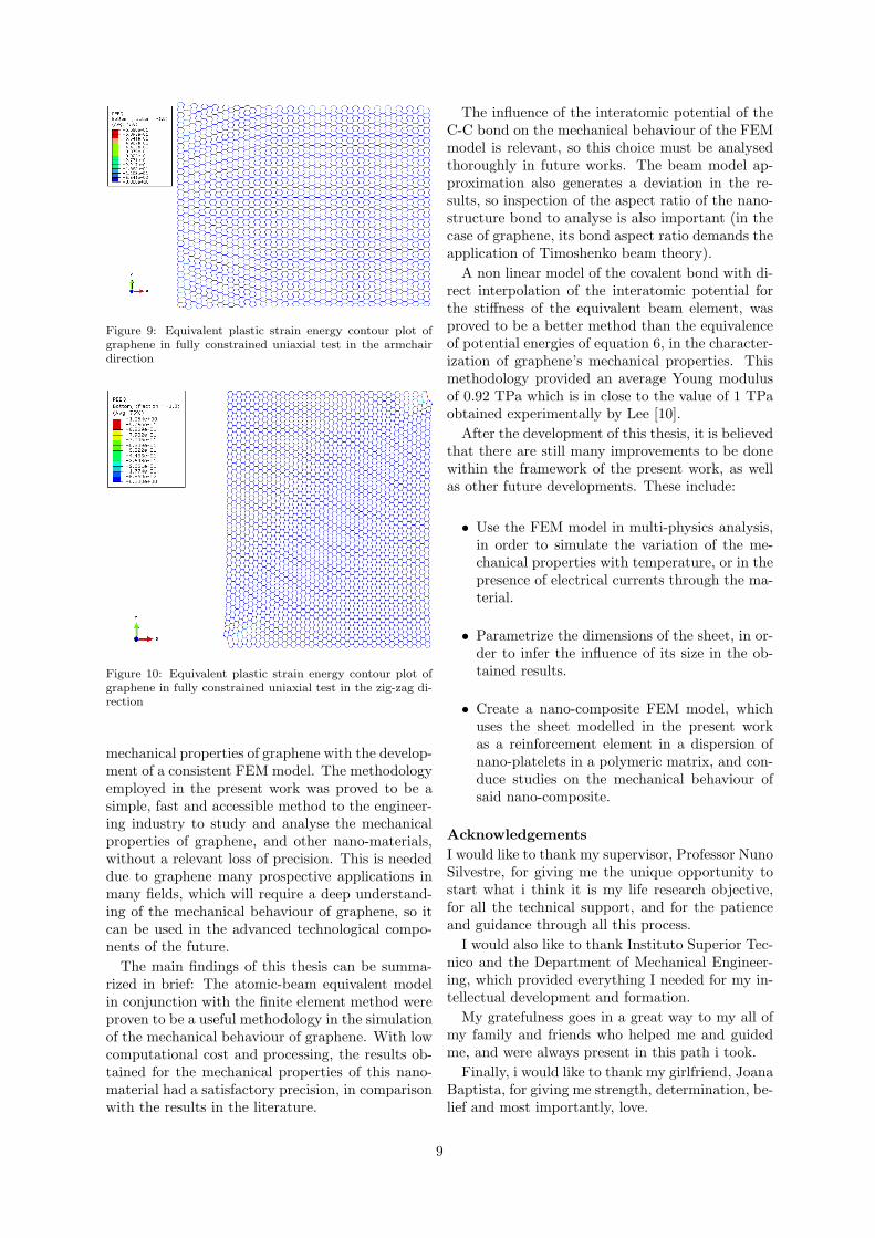
Figure 9: Equivalent plastic strain energy contour plot ofgraphene in fully constrained uniaxial test in the armchairdirection

Figure 10: Equivalent plastic strain energy contour plot ofgraphene in fully constrained uniaxial test in the zig-zag di-rection

mechanical properties of graphene with the develop-ment of a consistent FEM model. The methodologyemployed in the present work was proved to be asimple, fast and accessible method to the engineer-ing industry to study and analyse the mechanicalproperties of graphene, and other nano-materials,without a relevant loss of precision. This is neededdue to graphene many prospective applications inmany fields, which will require a deep understand-ing of the mechanical behaviour of graphene, so itcan be used in the advanced technological compo-nents of the future.

The main findings of this thesis can be summa-rized in brief: The atomic-beam equivalent modelin conjunction with the finite element method wereproven to be a useful methodology in the simulationof the mechanical behaviour of graphene. With lowcomputational cost and processing, the results ob-tained for the mechanical properties of this nano-material had a satisfactory precision, in comparisonwith the results in the literature.

The influence of the interatomic potential of theC-C bond on the mechanical behaviour of the FEMmodel is relevant, so this choice must be analysedthoroughly in future works. The beam model ap-proximation also generates a deviation in the re-sults, so inspection of the aspect ratio of the nano-structure bond to analyse is also important (in thecase of graphene, its bond aspect ratio demands theapplication of Timoshenko beam theory).

A non linear model of the covalent bond with di-rect interpolation of the interatomic potential forthe stiffness of the equivalent beam element, wasproved to be a better method than the equivalenceof potential energies of equation 6, in the character-ization of graphene’s mechanical properties. Thismethodology provided an average Young modulusof 0.92 TPa which is in close to the value of 1 TPaobtained experimentally by Lee [10].

After the development of this thesis, it is believedthat there are still many improvements to be donewithin the framework of the present work, as wellas other future developments. These include:

• Use the FEM model in multi-physics analysis,in order to simulate the variation of the me-chanical properties with temperature, or in thepresence of electrical currents through the ma-terial.

• Parametrize the dimensions of the sheet, in or-der to infer the influence of its size in the ob-tained results.

• Create a nano-composite FEM model, whichuses the sheet modelled in the present workas a reinforcement element in a dispersion ofnano-platelets in a polymeric matrix, and con-duce studies on the mechanical behaviour ofsaid nano-composite.

Acknowledgements

I would like to thank my supervisor, Professor NunoSilvestre, for giving me the unique opportunity tostart what i think it is my life research objective,for all the technical support, and for the patienceand guidance through all this process.

I would also like to thank Instituto Superior Tec-nico and the Department of Mechanical Engineer-ing, which provided everything I needed for my in-tellectual development and formation.

My gratefulness goes in a great way to my all ofmy family and friends who helped me and guidedme, and were always present in this path i took.

Finally, i would like to thank my girlfriend, JoanaBaptista, for giving me strength, determination, be-lief and most importantly, love.

9

References[1] High-resolution tem on graphene.

http://www.cen.dtu.dk/

english/Research/Projects/

ACTUAL-High-Resolution-TEM-on-graphene.Accessed: 16-04-2016.

[2] K. Alzebdeh. Evaluation of the in-plane effec-tive elastic moduli of single-layered graphenesheet. International Journal of Mechanics andMaterials in Design, 8:269–278, May 2012.

[3] N. Attig, K. Binder, and H. Grubm. Introduc-tion to molecular dynamics simulation. Com-putational Soft Matter: From Synthetic Poly-mers to Proteins, 23(2):1–28, 2004.

[4] O. L. Blakslee. Elastic constants of compres-sion annealed pyrolytic graphite. Journal ofApplied Physics, 41:3373, Aug. 1970.

[5] W. D. Cornell. A second generation force fieldfor the simulation of proteins, nucleic acids,and organic molecules. Journal of the Amer-ican Chemical Society, 117:5179–5197, Nov.1995.

[6] O. Frank. Development of a universal stresssensor for graphene and carbon fibres. Naturecommunications, 2:255, Mar. 2011.

[7] S.-J. Han, A. V. Garcia, S. Oida, and K. Jenk-ins. Graphene radio frequency receiver inte-grated circuit. Nature communications, 5:3086,Jan. 2014.

[8] Y. Huang. Thickness of graphene and single-wall carbon nanotubes. Physical Review B- Condensed Matter and Materials Physics,74:1–9, Dec. 2006.

[9] G. Kalosakas, N. N. Lathiotakis, C. Galiotis,and K. Papagelis. In-plane force fields and elas-tic properties of graphene. Journal of AppliedPhysics, 113(13), 2013.

[10] C. Lee and X. Wei. Measurement of the elasticproperties and intrinsic strenght of monolayergraphene. Science, 321:385–388, July 2008.

[11] F. Liu, P. Ming, and J. Li. Ab initio calcu-lation of ideal strength and phonon instabilityof graphene under tension. Physical Review B,76:064120, Aug. 2007.

[12] M. Meo and M. Rossi. Prediction of young’smodulus of single wall carbon nanotubes bymolecular-mechanics based finite element mod-elling. Composites Science and Technology,66:1597–1605, Feb. 2006.

[13] A. Merril. Sci-kit nano documentation, Nov2015. https://scikit-nano.org/doc/.

[14] K. Min and N. Aluru. Mechanical propertiesof graphene under shear deformation. AppliedPhysics Letters, 98:1–3, Jan. 2011.

[15] P. M. Morse. Diatomic molecules according tothe wave mechanics. ii. vibrational levels, 1929.

[16] Z. Ni and H. Bu. Anisotropic mechanicalproperties of graphene sheets from molecu-lar dynamics. Physica B: Condensed Matter,405:1301–1306, Nov. 2009.

[17] G. M. Odegard and T. S. Gates. Equivalent-continuum modeling of nano-structured ma-terials. Composites Science and Technology,62:1869–1880, Jan. 2002.

[18] F. Scarpa. The bending of single layergraphene sheets: the lattice versus continuumapproach. Nanotechnology, 21:125702, Mar.2010.

[19] O. Shenderova, V. Zhirnov, and D. W. Bren-ner. Carbon Nanostructures. Critical Reviewsin Solid State and Materials Sciences, 27 edi-tion, Aug 2006.

[20] J. Silvestre, N. Silvestre, and J. de Brito. Anoverview on the improvement of mechanicalproperties of ceramics nanocomposites. Jour-nal of Nanomaterials, 2015:13, 2015.

[21] M. D. Stoller, S. Park, Z. Yanwu, and J. An.Graphene-based ultracapacitors. Nano Letters,8(10):3498–3502, Oct. 2008.

[22] J. Tsai and J. Tu. Characterizing mechanicalproperties of graphite using molecular dynam-ics simulation. Materials and design, 31:194–199, June 2009.

[23] K. Zakharchenko and M. I. Katsnelson. Finitetemperature lattice properties of graphene be-yond the quasiharmonic approximation. Phys-ical Review Letters, 102:2–5, Jan. 2009.

[24] Y. Zhu, L. Li, and C. Zhang. A seamless three-dimensional carbon nanotube graphene hybridmaterial. Nature communications, 3(92):1225,Nov. 2012.

10