Mechanics and dynamics of translocating MreB filaments on

*For correspondence:

[email protected]

Competing interests: The

authors declare that no

competing interests exist.

Funding: See page 11

Received: 02 August 2018

Accepted: 15 February 2019

Published: 18 February 2019

Reviewing editor: Tam Mignot,

Aix Marseille University-CNRS

UMR7283, France

Copyright Wong et al. This

article is distributed under the

terms of the Creative Commons

Attribution License, which

permits unrestricted use and

redistribution provided that the

original author and source are

credited.

Mechanics and dynamics of translocatingMreB filaments on curved membranesFelix Wong1, Ethan C Garner2,3, Ariel Amir1*

1John A Paulson School of Engineering and Applied Sciences, Harvard University,Cambridge, United States; 2Department of Molecular and Cellular Biology, HarvardUniversity, Cambridge, United States; 3Center for Systems Biology, HarvardUniversity, Cambridge, United States

Abstract MreB is an actin homolog that is essential for coordinating the cell wall synthesis

required for the rod shape of many bacteria. Previously we have shown that filaments of MreB bind

to the curved membranes of bacteria and translocate in directions determined by principal

membrane curvatures to create and reinforce the rod shape (Hussain et al., 2018). Here, in order to

understand how MreB filament dynamics affects their cellular distribution, we model how MreB

filaments bind and translocate on membranes with different geometries. We find that it is both

energetically favorable and robust for filaments to bind and orient along directions of largest

membrane curvature. Furthermore, significant localization to different membrane regions results

from processive MreB motion in various geometries. These results demonstrate that the in vivo

localization of MreB observed in many different experiments, including those examining negative

Gaussian curvature, can arise from translocation dynamics alone.

DOI: https://doi.org/10.7554/eLife.40472.001

IntroductionThe role of membrane curvature in influencing the cellular location and function of proteins has been

increasingly appreciated (McMahon and Gallop, 2005; Zimmerberg and Kozlov, 2006;

Baumgart et al., 2011). In cells, membrane curvature can both be induced by proteins that bind to

membranes as well as recruit proteins that bind to this curvature (Peter et al., 2004; Renner and

Weibel, 2011; Wang and Wingreen, 2013; Ursell et al., 2014; Hussain et al., 2018; Wu et al.,

2018). Here, we focus on MreB, an actin homolog essential for coordinating the cell wall synthesis

required for the rod shape of many bacteria (Jones et al., 2001). We examine how MreB orientation

and motion along directions of principal curvature affect its localization in different cellular geome-

tries. MreB filaments polymerize onto membranes (Figure 1A) (Salje et al., 2011; van den Ent

et al., 2014; Hussain et al., 2018), creating short filaments that move along their lengths in live

cells. Viewed dynamically, MreB filaments are seen to rotate around the rod width, a motion pow-

ered by the activity of associated cell wall synthesis enzymes (Figure 1B and Figure 1—video 1)

(Garner et al., 2011; Domınguez-Escobar et al., 2011; van Teeffelen et al., 2011; Reimold et al.,

2013; Hussain et al., 2018). The orientation of MreB filaments coincides with the direction of their

motion, as filaments move along the direction in which they point (Figure 1C) (Hussain et al., 2018;

Olshausen et al., 2013). However, studies examining the localization of MreB in kymographs

(Ursell et al., 2014) or at single time points (Bratton et al., 2018) have found that, in Escherichia

coli, MreB filaments are enriched at regions of negative Gaussian curvature or small mean curvature

(Figure 1D). This prompts the question of how the collective motion of MreB filaments could affect,

or give rise to, their enrichment. As filaments are constantly moving, their instantaneous localization

to any one point is transient: a typical filament (~250 nm long) in Bacillus subtilis moves through a

1 mm2 region in ~30 s. To understand how the previously observed enrichment at negative Gaussian

Wong et al. eLife 2019;8:e40472. DOI: https://doi.org/10.7554/eLife.40472 1 of 30

RESEARCH ADVANCE

http://creativecommons.org/licenses/by/4.0/

http://creativecommons.org/licenses/by/4.0/

https://doi.org/10.7554/eLife.40472.001

https://doi.org/10.7554/eLife.40472

https://creativecommons.org/

https://creativecommons.org/

http://elifesciences.org/

http://elifesciences.org/

http://en.wikipedia.org/wiki/Open_access

http://en.wikipedia.org/wiki/Open_access

curvatures could arise from the dynamics of filaments moving around the cell, we sought to relate

the binding and motion of MreB filaments to their distribution in different geometries.

In previous work (Hussain et al., 2018), we demonstrated that MreB filaments orient and translo-

cate along directions of largest principal curvature inside differently shaped B. subtilis cells and lipo-

somes. To understand how MreB filaments orient along different membrane curvatures and how

their motion along this orientation affects their cellular localization, we first model the mechanics of

MreB-membrane binding and provide a quantitative description of how MreB filaments bind both in

vivo and in vitro. Next, we model the curvature-dependent motion of MreB filaments in different

geometries and examine how this motion affects their distribution to different membrane regions.

A

D

B

Vesicle

Filaments

Negative/Positive Gaussian curvature correlates with more/less MreB

–1–2 –1 0 21R

elat

ive

Mre

B e

nric

hmen

t

1.0

0.5

0

1.5

2.0

Average

Full distribution of observed MreB enrichment

90°

10 30 50 9070

Frac

tion

0.2

0.1

0.0

0.3

0.4MreB filaments alignedin B. subtilis protoplasts (n

MreB tracks in wild-type cells(n

C

Figure 1. Experimental observation of membrane binding and translocation. (A) Cryo-electron microscopy image showing the direct membrane

binding of MreB filaments reconstituted in vitro to vesicles. The scale bar indicates 50 nm, and dashed curves represent guides. The image is

reproduced here from Salje et al. (2011) under a CC BY 3.0 license (https://creativecommons.org/licenses/by/3.0/). (B) Fluorescence microscopy image

of MreB filaments translocating in live Bacillus subtilis cells with trajectories of individual filaments drawn and cell edges outlined, reproduced from

Hussain et al. (2018) (see also Figure 1—video 1). Note that typical trajectories are perpendicular to the cellular long axis, consistent with the binding

angles in (C). The scale bar indicates 1 mm. (C) Angular distribution of membrane-bound filaments within B. subtilis protoplasts confined to become

rod-shaped (green curve) and MreB motion in wild-type B. subtilis cells (black curve), reproduced from Hussain et al. (2018). (D) Relative MreB

enrichment in Escherichia coli cells growing in a sinusoidally shaped chamber, adapted from Ursell et al. (2014).


The following video is available for figure 1:

Figure 1—video 1. SIM-TIRF movies of MreB motion.



Research advance Microbiology and Infectious Disease Physics of Living Systems

https://creativecommons.org/licenses/by/3.0/




Strikingly, we find that the dynamics of MreB translocation alone, without requiring any intrinsic pref-

erence of MreB filaments for curved regions of the cell, results in differential enrichment of MreB fila-

ments at regions of negative Gaussian curvature or small mean curvature similar to those observed

in cells.

Results

Mechanics of bindingWe first model how inwardly curved (Salje et al., 2011; van den Ent et al., 2014; Hussain et al.,

2018) MreB filaments bind and orient on membranes. Previous theoretical studies have modeled the

binding of protein filaments to membranes and demonstrated that binding conformations can be

influenced by both filament thickness and twist. In a seminal theoretical work, Wang and Wingreen

modeled twisted bundles of MreB approximately six-fold thicker than typical filaments (Wang and

Wingreen, 2013). This study nicely demonstrated that the mechanics of binding alone could orient

bundles and suggested that bundle length could be limited by twist. Another elegant theoretical

study by Quint et al. demonstrated that twisted filaments of varying rigidities could bind to regions

of negative Gaussian curvature in manners that are particularly energetically favorable (Quint et al.,

2016). While it is intriguing to examine the effects of filament rigidity and twist on general filament

systems (discussed below), here we focus on modeling thin, inwardly curved MreB filaments with no

twist. We focus on these parameters as they reflect the observations of all available in vitro studies

of membrane-associated MreB: three different cryo-electron microscopy studies have shown that

membrane-bound MreB filaments are flat and untwisted, binding to the membrane on one filament

face (Figure 1A) (Salje et al., 2011; van den Ent et al., 2014; Hussain et al., 2018). These studies

also suggest that inward curvature, and not twist, limits filament length: MreB filaments are short

when polymerized onto non-deforming planar-supported lipid bilayers, but become extremely long

when polymerized inside deformable liposomes (Salje et al., 2011; van den Ent et al., 2014;

Hussain et al., 2018). The model we present here extends our previous work (Hussain et al., 2018)

and demonstrates that thin, untwisted filaments orient robustly along directions of largest principal

curvature, thus providing a generic mechanism for orienting their motion.

We model an MreB filament as a polymer which binds linearly along its length to a membrane in

an energetically favorable manner, namely via burial of hydrophobic residues on one face

(Figure 2A; see Figure 2—figure supplement 1 for additional details) (Salje et al., 2011). We

assume the filament to be a curved, cylindrical, linear-elastic rod which is free to bend to maximize

membrane interaction, so that its elastic energy of deformation is Ebend ¼ ðpYr4f =8Þ �R ðk� ksÞ2d‘,

where rf is the filament cross-sectional radius, Y is the filament Young’s modulus, k is the curvature

of the deformed state, ks is the intrinsic filament curvature, and the integration is over the filament

length (Landau and Lifshitz, 1970). We will minimize the free energy change due to binding with

respect to the deformed curvature, k.

Next, we assume an isotropic, fluid, bilayer membrane, where there are no in-plane shears and

the only in-plane deformations are compressions and expansions (Safran, 2003). The membrane

free energy is given by the Helfrich form,

F ¼ZS

kb2ð2H�HsÞ2þ kt

2Kþg

� �dA� p

ZSdV ; (1)

where kb is the bending rigidity of the membrane, kt is the saddle-splay modulus of the membrane,

Hs is the spontaneous curvature, g is the membrane surface tension, p is the pressure difference

across the membrane, H and K are the mean and Gaussian curvatures of the membrane surface, S,respectively, and dA and dV denote area and volume elements, respectively (Helfrich, 1973;

Safran, 2003; Zhong-can and Helfrich, 1987; Zhong-can and Helfrich, 1989). For the small mem-

brane deformations considered in this work, we assume that excess phospholipids can be freely

added to the membrane to compensate for stretching, so that the membrane surface tension

g¼ 0 (Safran, 2003). Note that a nonzero surface tension would make the preferred binding orienta-

tion determined below more energetically favorable. For simplicity, we also assume Hs ¼ 0 and note

that the case of a nonzero Hs can be considered similarly. Finally, we assume that the membrane




surface can be parameterized in the Monge gauge by a function h¼ hðx;yÞ, where x and y are real

numbers and terms of quadratic order or higher in the gradient of h, rh, are neglected. As shown in

Appendix 1, the mechanical energy associated with membrane deformations is determined by the

solution of the shape equation

D2h¼ pkb; (2)

which is similar to the equilibrium equation of a thin plate (Ventsel and Krauthammer, 2001;

Timoshenko and Woinowsky-Krieger, 1959). Here D2 is the biharmonic operator and Equation (2)

is subject to Dirichlet boundary conditions enforcing continuity of mean curvature and surface height

in a manner compatible with the deformed filament. Equation (2) can then be decomposed as two

Poisson equations, each with Dirichlet boundary conditions, and solved numerically using the finite

element method (Appendix 1).

The free energy change due to filament binding is determined by Ebend, F , and the solution of

Equation (2). For characteristic parameter values relevant to the binding of MreB filaments to bacte-

rial membranes, as summarized in Supplementary file 1, our model predicts a preferred, circumfer-

ential orientation of MreB binding in a rod-shaped cell. This result arises because the intrinsic

curvature of filaments is smaller than characteristic cell radii. While the filament bends to conform to

the membrane for physiological values of p—as shown in previous work (Hussain et al., 2018)—and

A Undeformed

B

EbendInteraction

energy gainedfrom binding

p

Polymerbends

Membranebends

No binding

In vivo(Cell membranes)

In vitro(Vesicles)

Criticalpressure

Free

ene

rgy

chan

gedu

e to

bin

ding

(kT)

Binding angle – 90°45°–45°

p = 0.2 atm, 20 atmR

C

Proteinfilament

Deformed

Membrane

–465

–495

–475

–485

–455

–90° 90°0°

Rcell

cell

Figure 2. Mechanics of binding. (A) A schematic of the model. A protein filament (red) may bend and bind to a cylindrical membrane (green) at an

angle with respect to the long axis, �, and the equilibrium conformation may involve deformations of both protein and membrane. (B) Plot of the

estimated free energy change due to filament binding against the binding angle, �, where the cell radius Rcell ¼ 0:5 �m, the pressure difference across

the membrane p ¼ 20 atm, the estimated turgor pressure of B. subtilis (Whatmore and Reed, 1990), and the other model parameters are given in

Supplementary file 1. The estimate is similar for p ¼ 0:2 atm, but exhibits a more shallow potential well for Rcell ¼ 1:5 �m (red curve). (C) An

approximate phase diagram of protein-membrane binding. The dashed lines delineate regimes, as explained further in Appendix 1.


The following figure supplement is available for figure 2:

Figure supplement 1. Energetic modeling of MreB binding and deformation of vesicles.







grossly deforms the membrane for small values of p, the preferred binding orientation is robust to

changes in p (Figure 2B). In fact, across a wide range of parameter values including the filament

bending rigidity (B ¼ pYr4f =4), the filament intrinsic curvature (ks), and the membrane pressure differ-

ence (p), a preferred binding orientation exists and coincides with the direction of largest principal

curvature for any membrane which is less curved than the filament. In the case of p ¼ 0, as discussedin Appendix 1, the prediction that MreB binding induces large membrane deformations is consistent

with cryo-electron microscopy images of MreB binding to vesicles (Figure 1A) (Salje et al., 2011;

van den Ent et al., 2014). Importantly, the energetic penalties for deviatory binding conformations

are larger than the energy of thermal fluctuations across a large range of p, suggesting the empiri-

cally observed variation in binding orientation (Figure 1C) to be caused by other sources of stochas-

ticity. The energetic penalties are also decreased in wider membranes for both small and

physiological values of p, the latter of which is consistent with the gradual widening of the distribu-

tions of MreB trajectory angles in wider B. subtilis protoplasts (Hussain et al., 2018).

In general, the mechanics of filament binding are well described by the pressure difference across

the membrane and the filament bending energy, which can be viewed as order parameters that

largely dictate whether the filament predominantly bends the membrane, bends to conform to the

membrane, or both. An approximate phase diagram for MreB binding to any membrane which is

less curved than the filament can be determined (Figure 2C and Appendix 1). Below, we suppose

the membrane surface to be less curved than the filament—so that it is always energetically favor-

able to orient along directions of largest membrane curvature—and model filament translocation

along these directions.

Dynamics of translocationWe next examine how the translocation of MreB filaments, once bound to the membrane, affects

their distribution in different geometries. Inside cells, MreB filaments move along the membrane in

the direction of their orientation (Hussain et al., 2018; Olshausen et al., 2013) (Figure 1C). This

directional and processive motion is driven by cell wall synthesis (Sliusarenko et al., 2010;

van Teeffelen et al., 2011; Olshausen et al., 2013), and filaments may reorient according to differ-

ent membrane geometries (Hussain et al., 2018). Thus, highly-bent MreB filaments translocate

along the direction of largest curvature, a direction that minimizes the energetic cost of binding. As

discussed below, this hypothesis is supported by observations that (1) MreB moves circumferentially

in live B. subtilis cells, but this motion becomes disoriented if cells become round, (2) circumferential

motion is re-established when round cells are confined into rods, (3) MreB moves directionally in

bulges protruding from round cells, and (4) MreB filaments rapidly translocate out of poles in rods,

reorienting when filaments reach the cylindrical bulks (Hussain et al., 2018). Assuming translocation

on a static surface, we may model the trajectories of filaments as biased random walks as follows

(with more details provided in Appendix 1). The case of a dynamical surface, as expected for MreB-

directed growth, can be considered similarly. Note that a ‘biased random walk’ refers to a succes-

sion of random steps which may be processive: while the mean-squared displacement of a filament

will be approximately quadratic, and not linear, in time, the processive motion we consider is ran-

dom only because the translocation direction can deviate from directions of largest membrane cur-

vature due to sources of stochasticity (Figure 1C). We will show that our biased random walk model

of filament trajectories leads to predictions of MreB localization.

We consider the membrane as a parametric surface, r ¼ rðu; vÞ, embedded in three-dimensional

space (R3) with surface coordinates u and v and a filament as a point on this surface which, at any

moment in time, translocates along the largest principal direction d—that is, the direction of largest

curvature of the surface. As d is a vector in R3, arbitrarily moving in the direction of d may move the

filament off of the surface. To define the translocation consistently, we

set h ¼ cos�1 d�r�jjdjj�jjr� jj, where h is an angular deviation from the largest principal direction on the sur-

face introduced by possible sources of stochasticity, the modified direction corresponds to an

angle � relative to the u-axis in parametric coordinates, r� 2 R3 is the derivative of r in the direction

of �, and distances are defined by the surface metric. Translocating along an angle � with respect to

the u-axis in ðu; vÞ-coordinates then ensures that the filament remains on the surface, and the direc-

tion of translocation corresponds to that on a patch of r.




As a discrete-time flow in ðu; vÞ-coordinates, and with suitable units of time so that the filament

may reorient at every timestep, the 2D equation of filament motion is

Xnþ1 ¼ Xn þ�n‘nðcos�n; sin�nÞ; (3)

where Xn, ‘n, and �n are the position, step size, and translocation angle, respectively, of the filament

at a timestep n. Here �n is the value of � computed at the surface point corresponding

to Xn and assuming h~Nð0;s2Þ—that is, the angular noise is normally-distributed, with mean zero

and a variance, s2, to be inferred from data—and note that the translocation noise, s, may depend

on quantities such as the principal curvatures, as discussed later. �n is a random sign, which accounts

for the possibility of both left-handed and right-handed translocation, and may not substantially vary

in n if the filament does not backtrack, as is assumed for the remainder of this work. We assume that

‘n satisfies an integral equation which relates it to a constant and finite filament step size, L, on the

surface (Appendix 1), and note that inertia in MreB motion, as measured previously by the velocity

autocorrelation (Kim et al., 2006; van Teeffelen et al., 2011), is modeled by the finite step size.

Note that, when both principal curvatures are equal, so that d is not well defined, we will assume

steps of uniformly random angles and size L on the surface. Furthermore, for finite step sizes, Equa-

tion (3) extrapolates the translocation direction in surface coordinates: while motion along the larg-

est principal direction can be maintained irrespective of parameterization by parallel transport, we

anticipate the distinction from Equation (3) to be insignificant for many geometries due to the small

step sizes considered in this work. Determining the probability distribution of X then determines the

probability distribution of the filament on r, and this can be done analytically and numerically for sev-

eral geometries as discussed below.

We next consider the dynamics of activating and deactivating filaments as follows. We suppose

that a filament may be activated at a position X at any timestep at a constant rate k � 0 with proba-

bility proportional to the membrane surface area, dAðXÞ, and deactivated at a constant rate l � 0which determines the filament’s processivity—that is, the mean number of steps that a filament takes

on the membrane surface before becoming inactive (Figure 3A). The case of k being dependent on

fields, such as mechanical strains (Wong et al., 2017), can be considered similarly but is not neces-

sary for the results below. An ensemble of filaments produced by such dynamics will exhibit filament

numbers, NF, that vary in space and time, and likewise for the filament concentration

CFðX; nÞ ¼ NFðX; nÞ=dAðXÞ. Below, we discuss characteristic parameter values relevant to MreB and

show that the dynamics of Equation (3) gives rise to localization. We then examine the model in

detail and describe how localization depends on different parameters of the model.

Implications to MreB localizationPrevious fluorescence microscopy measurements provide estimates for the step size (L), deactivationrate (l), and translocation noise (s) of MreB filaments in cells. We assume L to be 200 nm as a model-

ing choice, but show in Appendix 1 that the results discussed below are qualitatively similar for sig-

nificantly larger L ( ~ 2�m). Similar experiments have estimated the persistence time of MreB

filaments in E. coli as ~5 min (Ursell et al., 2014), while a characteristic translocation noise of

s » 0:3 rad in B. subtilis has been found separately by (1) measuring filament trajectory angles relative

to the midline and (2) measuring binding angles in confined protoplasts (Figure 1C) (Hussain et al.,

2018). While we assume the values of l and s to be based on these measurements, we examine the

effects of varying l and s in the following section. Furthermore, in recent studies, rod-shaped cells

have been perturbed to be in geometries other than a spherocylinder (Ursell et al., 2014;

Wong et al., 2017; Hussain et al., 2018; Renner et al., 2013; Amir et al., 2014). As the distribution

of MreB filament angles gradually becomes broader as B. subtilis cells become wider

(Hussain et al., 2018), it may also be reasonable to suppose that s depends on the difference, Dc,of principal curvatures at the location of any MreB filament: s ¼ aðDcÞ�1, where a » 0:6 rad � �m�1 is a

constant of proportionality determined by experimental data. While all our results pertaining to

MreB below assume this dependence as to be consistent with data, we show in Appendix 1 that our

results are similar for different dependencies of s on Dc.Given the aforementioned parameters, Equation (3) leads to predictions for the statistics of the

filament position (X) and the ensuing filament concentration (CF) across different membrane geome-

tries. For a cylindrical cell, analytical expressions for the statistics of X show that translocation noise




B

E F

–0.6 –0.4 –0.2 0 0.2 0.40

2

4

6

8

10

12

0.6

Freq

uenc

y

n = 47

Experiment Theory

Simulation

Filament concentration

CFilam

ent concentration

2×

0×

2×0×

Cell membrane

Translocation direction of filament

Activation (k

Deactivation (

Principal directions

A

G

Positive/N

egative Gaussian curvature

Finite Continuum

Filament concentration0× 2×

Bratton et al. (wild-type

0.0 0.4 0.8 1.2 1.6 2.0 2.4 2.80.0

0.5

1.0

1.5

2.0

2.5

3.0

0.0 2.0 4.0 6.00.0

0.5

1.0

1.5

2.0

2.5

3.0

–2.0

Ursell et al.(confined/unconfined

Shi et al.(thin/wide

Continuum

Finite

Finite

Continuum

–2–1

D

Negative Gaussian curvature Positive Gaussian curvature


1.1×0.9×

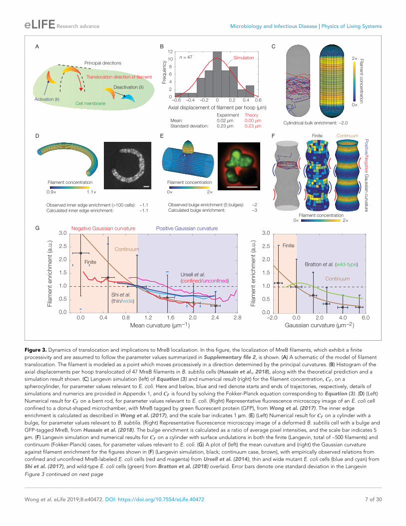
Figure 3. Dynamics of translocation and implications to MreB localization. In this figure, the localization of MreB filaments, which exhibit a finite

processivity and are assumed to follow the parameter values summarized in Supplementary file 2, is shown. (A) A schematic of the model of filament

translocation. The filament is modeled as a point which moves processively in a direction determined by the principal curvatures. (B) Histogram of the

axial displacements per hoop translocated of 47 MreB filaments in B. subtilis cells (Hussain et al., 2018), along with the theoretical prediction and a

simulation result shown. (C) Langevin simulation (left) of Equation (3) and numerical result (right) for the filament concentration, CF , on a

spherocylinder, for parameter values relevant to E. coli. Here and below, blue and red denote starts and ends of trajectories, respectively, details of

simulations and numerics are provided in Appendix 1, and CF is found by solving the Fokker-Planck equation corresponding to Equation (3). (D) (Left)

Numerical result for CF on a bent rod, for parameter values relevant to E. coli. (Right) Representative fluorescence microscopy image of an E. coli cell

confined to a donut-shaped microchamber, with MreB tagged by green fluorescent protein (GFP), from Wong et al. (2017). The inner edge

enrichment is calculated as described in Wong et al. (2017), and the scale bar indicates 1 mm. (E) (Left) Numerical result for CF on a cylinder with a

bulge, for parameter values relevant to B. subtilis. (Right) Representative fluorescence microscopy image of a deformed B. subtilis cell with a bulge and

GFP-tagged MreB, from Hussain et al. (2018). The bulge enrichment is calculated as a ratio of average pixel intensities, and the scale bar indicates 5

mm. (F) Langevin simulation and numerical results for CF on a cylinder with surface undulations in both the finite (Langevin, total of ~500 filaments) and

continuum (Fokker-Planck) cases, for parameter values relevant to E. coli. (G) A plot of (left) the mean curvature and (right) the Gaussian curvature

against filament enrichment for the figures shown in (F) (Langevin simulation, black; continuum case, brown), with empirically observed relations from

confined and unconfined MreB-labeled E. coli cells (red and magenta) from Ursell et al. (2014), thin and wide mutant E. coli cells (blue and cyan) from

Shi et al. (2017), and wild-type E. coli cells (green) from Bratton et al. (2018) overlaid. Error bars denote one standard deviation in the Langevin

Figure 3 continued on next page




does not significantly affect the mean or variance of the circumferential displacement of a filament

(Appendix 1). In contrast, the value of s » 0:3 rad corresponds to a standard deviation of approxi-

mately 0:2 �m for the axial displacement of a filament per hoop of wall material inserted. This value

is consistent with experimental measurements (Figure 3B), showing that deviations from a circumfer-

ential translocation direction can significantly contribute to wall insertions in the axial direction and

disordered wall architecture.

MreB filaments have been observed to be depleted from the hemispherical poles of spherocylin-

drical cells compared to the cylindrical bulks (Kawazura et al., 2017; Ursell et al., 2014). Observa-

tions of filament dynamics revealed a possible explanation: MreB filaments reorient rapidly in, and

translocate out of, the poles and into the bulks, where motion then becomes aligned (Hussain et al.,

2018). Consistent with this observation, simulations of Equation (3) on a spherocylindrical surface

show that the concentration of filaments in the bulk is enhanced (Figure 3C). The average filament

concentration is predicted to be approximately two-fold higher in the bulk than the poles, in agree-

ment with experimental measurements in E. coli (Ursell et al., 2014). Simulations of Equation (3) on

a toroidal surface are also quantitatively consistent with prior measurements of MreB fluorescence in

E. coli cells confined to donut-shaped microchambers, which have shown that MreB intensity is

increased at the inner edges by a factor of ~1.1 relative to the midlines (Figure 3D) (Wong et al.,

2017). For a spherocylinder, filament enrichment arises because the cylindrical bulk retains filaments:

oriented motion is preserved in the bulk, while disordered motion at the poles eventually becomes

ordered. In contrast, filament enrichment arises in a curved cell because filaments become uniformly

distributed along circumferential hoops. The smaller arclength along the inner edge then results in a

greater density of filaments.

In our previous study, we found that MreB rotation and localization at small protrusions in B. sub-

tilis protoplasts preceded rod shape generation from these protrusions (Hussain et al., 2018). To

model the geometry observed in these experiments, we consider a cylindrical body with a protrud-

ing bulge in which filament trajectories become parallel to the cylinder long axis. Simulations of

Equation (3) on this geometry reveal that the filament concentration is larger in the bulge and that

the predicted enrichment is quantitatively consistent with the MreB enhancement observed in

bulged cells, without any fitting parameters (Figure 3E and Figure 3—figure supplement 1). Similar

to the case of a spherocylinder, localization arises due to the bulge attracting filaments. The dynam-

ics of Equation (3) therefore results in localization which contributes to de novo generation of rod

shape.

Finally, previous work has examined MreB localization in E. coli cells (1) with submicron-scale

shape fluctuations or (2) confined in sinusoidal chambers (Ursell et al., 2014; Shi et al., 2017;

Bratton et al., 2018). The empirically observed magnitudes of MreB enrichment at regions of nega-

tive Gaussian curvature or small mean curvature in these studies are consistent with our modeling.

To model the cell shapes observed in these experiments, we consider filament translocation on a

geometry with both negative and positive Gaussian curvatures and undulations of smaller wave-

lengths than the surface size (Figure 3F and Figure 3—figure supplement 2). As discussed in

Appendix 1, the Gaussian and mean curvatures in this geometry are positively correlated and consis-

tent with experimental observations (Ursell et al., 2014). For this geometry, filament translocation

results in increased values of concentration (CF ) at regions of negative Gaussian curvature or small

Figure 3 continued

simulation, and 1 a.u. equals the mean of CF when the mean curvature is 1 mm�1 (left) and when the Gaussian curvature is 0 mm�2 (right). Note that the

magenta and green curves are not normalized according to this convention.


The following figure supplements are available for figure 3:

Figure supplement 1. Curvature-based translocation on cylinders with bulges.


Figure supplement 2. Correlations between Gaussian and mean curvatures for, and translocation directions in, cylinders with undulations of different

wavelengths.


Figure supplement 3. Effects of curvature-dependent translocation noise and varying filament properties on model predictions.









mean curvature (Figure 3F). This effect arises because the principal curvatures away from these

regions reorient filaments axially, instead of circumferentially, so that regions of negative Gaussian

curvature or small mean curvature attract filaments. Furthermore, the magnitude of this enhance-

ment is consistent with the amount of MreB enrichment observed (Figure 3G and Figure 3—figure

supplement 3), demonstrating that translocation dynamics alone can negatively correlate filament

concentration with Gaussian or mean curvature in cells with similar short wavelength undulations.

Dependence of localization on processivity and Gaussian curvatureAs we anticipate our model to be applicable to general filament systems, we now explore the

response of the filament concentration (CF) to (1) different parameter values and (2) other geome-

tries. We fix the filament step size (L) and suppose the translocation noise (s) and the deactivation

rate (l) to be constants which are varied within a broad range. We show in Appendix 1 that, for any

value of processivity and zero translocation noise, CF is uniform over the surface of an ellipsoid, as is

generally the case for any surface when the processivity is small (or, equivalently, l is large). In con-

trast, in the case of small l corresponding to large processivity—a limiting case that is relevant to

MreB—and over a range of s, CF is larger at the inner edge of a torus, at the inner edge of a helix,

and at the tips of an ellipsoid (Figure 4A and Figure 4—figure supplements 1 and 2). As discussed

above, localization occurs geometrically in these cases due to the filament number (NF) becoming

uniform over the surface and spatial variations in the surface area element. The magnitude of the

localization can be quantitatively predicted by geometric parameters alone (Appendix 1). The mech-

anism underlying localization is different for a spherocylinder or a bulged cylinder, for which surface

regions attract filaments. Nevertheless, a nonzero processivity is required for localization even in

geometries which attract filaments (Figure 4B and Figure 4—figure supplements 1 and 2).

Since filament enrichment depends on both processivity and geometry, we wondered if the locali-

zation of processive filaments always correlates with the Gaussian or mean curvatures, regardless of

overall geometry. Although Figure 3G demonstrates that filament enrichment correlates with nega-

tive Gaussian curvature or small mean curvature in a specific, undulating geometry, this correlation is

reversed in bulged cylinders (Figure 3E). Furthermore, Figure 4C illustrates a surface of zero Gauss-

ian curvature exhibiting regions which attract filaments, as filaments change from moving circumfer-

entially to moving axially in such regions (see Figure 4—figure supplement 3 for additional details).

Examining Equation (3) on different surfaces therefore shows that CF need not depend on Gaussian

curvature at all, and the dynamics modeled in this work cannot act as a generic mechanism for sens-

ing Gaussian curvature.

Finally, while large filament bundles or twist have not been observed in MreB filaments reconsti-

tuted in vitro (Salje et al., 2011; van den Ent et al., 2014; Hussain et al., 2018), it is possible that

general filament systems could exhibit these properties (Wang and Wingreen, 2013; Quint et al.,

2016). The binding and activation of twisted filaments may also depend on membrane Gaussian cur-

vature, as previously demonstrated (Quint et al., 2016). We systematically explore the effects of

varying filament bending rigidity, filament twist, and Gaussian curvature-dependent activation in

Appendix 1, where we show that our model predictions remain largely robust across a broad range

of these parameters (Figure 4—figure supplement 4). Thus, we expect filament dynamics to con-

tribute to localization in different filament systems, regardless of the details of filament rigidity, twist,

and other parameters of our model.

DiscussionAn outstanding problem in bacterial physiology has been to understand how short and disconnected

filaments distribute themselves within cells to conduct different cellular functions (Eun et al., 2015).

In this work, we have examined an aspect of this problem by modeling the direct binding of protein

filaments to membranes and the curvature-based translocation of an ensemble of such filaments.

Our results provide a theoretical framework for prior work examining MreB dynamics and localiza-

tion (Hussain et al., 2018; Salje et al., 2011; Wong et al., 2017; Ursell et al., 2014; Shi et al.,

2017; Bratton et al., 2018; Renner et al., 2013). Furthermore, our results are consistent with the

cellular localization observed in all these works and demonstrate that filament motion alone can cor-

relate enrichment with Gaussian curvature in specific geometries. Our work may be extended by

modeling an evolving membrane surface, as expected for MreB-directed growth, and it would be




intriguing to explore whether and how principal curvature-based translocation contributes to deter-

mining cell width.

The main contribution of this work is to show that the biological results of MreB localization, as

observed in many different experiments involving a range of cell shapes (Hussain et al., 2018;

Wong et al., 2017; Ursell et al., 2014; Shi et al., 2017; Bratton et al., 2018), can arise from proc-

essivity and principal curvature-dependent motion alone. Our study therefore helps to unravel how

rod shape formation may be achieved through subcellular-scale mechanisms (Amir and van Teeffe-

len, 2014; Shi et al., 2018; Surovtsev and Jacobs-Wagner, 2018). More broadly, our work shows

that the localization of translocating protein filaments can vary significantly depending on membrane

geometry. This paves the way for exploring similar behavior in other contexts, such as bacterial cyto-

kinesis and eukaryotic membrane trafficking and transport. For example, in bacterial cytokinesis,

A

C

B


0.5×

2×

Per

cent

age

offil

amen

ts a

t bul

ge

Zeroprocessivity

Infiniteprocessivity

Spherical bulge Ellipsoidal bulge

Filament concentration0× 2×

Zero processivity

Infinite processivity

Trajectories

0

10

20

30

40 Processivity

00

Figure 4. Dependence of localization on processivity and Gaussian curvature. (A) Langevin simulations of Equation (3) and numerical results for CF , the

filament concentration, on different surfaces. Note that cases of zero processivity correspond to uniform distributions and that we have considered the

limiting cases of zero and infinite processivity, along with a constant value of the translocation noise (s), here. Figure 3 shows numerical results for the

case of a large, but finite, processivity and a principal curvature-dependent translocation noise relevant to MreB. (B) Plot of the percentage of total

filaments contained in a bulge, for the two different geometries indicated in the limits of zero and infinite processivity. (C) Langevin simulation and

numerical result for CF on a non-circular cylinder in the limits of zero and infinite processivity.


The following figure supplements are available for figure 4:

Figure supplement 1. Curvature-based translocation on a torus and a helix.


Figure supplement 2. Curvature-based translocation on an ellipsoid.


Figure supplement 3. Curvature-based translocation on a geometry with zero Gaussian curvature.


Figure supplement 4. Effects of filament twist, flexural rigidity, and Gaussian curvature-dependent activation on model predictions.










filaments of the tubulin homolog FtsZ assemble at, and treadmill around, the septum, a process

which directs the insertion of new PG and constricts the cell (Bisson-Filho et al., 2017; Yang et al.,

2017). Like MreB, FtsZ filaments are curved and could orient along the largest principal direction on

membranes through bending alone (Osawa et al., 2009; Erickson et al., 2010). Treadmilling along

such directions would then allow filaments to drive PG synthesis circumferentially at the septum.

Aside from MreB and FtsZ, septins, BAR-domain-containing proteins, dynamins, and endopro-

teins are known to exhibit similar, curvature-dependent membrane binding behaviors important for

membrane trafficking, growth, and movement in both prokaryotes and eukaryotes (Baumgart et al.,

2011; Zimmerberg and Kozlov, 2006; McMahon and Gallop, 2005; Peter et al., 2004; Low and

Lowe, 2006; Raiborg and Stenmark, 2009; Teo et al., 2006; Kostelansky et al., 2007). Like MreB

filaments, many such proteins sense membrane curvature through mechanical deformations of either

the membrane or the protein itself. Unlike MreB or FtsZ, these proteins do not translocate; rather,

they often induce membrane curvature to facilitate downstream processes. One example is BAR-

domain-containing proteins, which scaffold higher-order assemblies of dynamin that actively con-

strict for vesicle scission (McMahon and Gallop, 2005). It would be interesting to apply the methods

introduced here to this and other biological systems where molecules are known to bind to mem-

branes or sense membrane curvature. These systems are widespread and involved in pathogenesis

(Baumgart et al., 2011; Frost et al., 2009), cell division (Renner et al., 2013; Ramamurthi and

Losick, 2009; Ramamurthi et al., 2009; Frost et al., 2009), intracellular trafficking

(Zimmerberg and Kozlov, 2006; McMahon and Gallop, 2005; Raiborg and Stenmark, 2009;

Ford et al., 2002; Frost et al., 2009; Romer et al., 2007), and cell migration (Frost et al., 2009;

Zhao et al., 2013). The mathematical model introduced in this work, which requires minimal

assumptions as to how filaments bind to and translocate on membranes, should be widely applicable

to these and other broader contexts.

AcknowledgementsFW was supported by the National Science Foundation Graduate Research Fellowship under grant

no. DGE1144152 and the Quantitative Biology Initiative at Harvard. ECG was supported by the

National Institutes of Health under grant no. DP2AI117923-01, the Smith Family Award, and the

Searle Scholar Fellowship. AA was supported by the Materials Research and Engineering Center at

Harvard, the Kavli Institute for Bionano Science and Technology at Harvard, and the Alfred P Sloan

Foundation. ECG and AA were supported by the Volkswagen Foundation. We thank Carl Wivagg,

Saman Hussain, Ned Wingreen, and Siyuan (Steven) Wang for discussions and Sven van Teeffelen,

Jie Lin, and Po-Yi Ho for comments on the manuscript.

Additional information

Funding

Funder Grant reference number Author

National Science Foundation DGE1144152 Felix Wong

Quantitative Biology Initiativeat Harvard

Felix Wong

National Institutes of Health DP2AI117923-01 Ethan C Garner

Smith Family Award Ethan C Garner

Searle Scholar Fellowship Ethan C Garner

Volkswagen Foundation Ethan C GarnerAriel Amir

Materials Research and Engi-neering Center at Harvard

Ariel Amir

Kavli Institute for BionanoScience and Technology atHarvard

Ariel Amir




Alfred P. Sloan Foundation Ariel Amir

The funders had no role in study design, data collection and interpretation, or the

decision to submit the work for publication.

Author contributions

Felix Wong, Conceptualization, Software, Formal analysis, Validation, Investigation, Visualization,

Methodology, Writing—original draft, Writing—review and editing; Ethan C Garner, Conceptualiza-

tion, Formal analysis, Funding acquisition, Investigation, Methodology, Writing—original draft, Writ-

ing—review and editing; Ariel Amir, Conceptualization, Formal analysis, Supervision, Funding

acquisition, Investigation, Methodology, Writing—original draft, Writing—review and editing

Author ORCIDs

Felix Wong http://orcid.org/0000-0002-2309-8835

Ethan C Garner https://orcid.org/0000-0003-0141-3555

Ariel Amir http://orcid.org/0000-0003-2611-0139

Decision letter and Author response

Decision letter https://doi.org/10.7554/eLife.40472.023

Author response https://doi.org/10.7554/eLife.40472.024

Additional files

Supplementary files. Supplementary file 1. Variables used, or calculated, in the model of filament binding and their

numerical values.


. Supplementary file 2. Variables used, or calculated, in the model of filament translocation and their

numerical values for E. coli.


. Transparent reporting form


Data availability

All data generated or analyzed during this study are included in the manuscript and supporting files.

ReferencesAmir A, Babaeipour F, McIntosh DB, Nelson DR, Jun S. 2014. Bending forces plastically deform growing bacterialcell walls. PNAS 111:5778–5783. DOI: https://doi.org/10.1073/pnas.1317497111, PMID: 24711421

Amir A, van Teeffelen S. 2014. Getting into shape: how do rod-like bacteria control their geometry? Systems andSynthetic Biology 8:227–235. DOI: https://doi.org/10.1007/s11693-014-9143-9, PMID: 25136385

Baumgart T, Capraro BR, Zhu C, Das SL. 2011. Thermodynamics and mechanics of membrane curvaturegeneration and sensing by proteins and lipids. Annual Review of Physical Chemistry 62:483–506. DOI: https://doi.org/10.1146/annurev.physchem.012809.103450, PMID: 21219150

Bisson-Filho AW, Hsu YP, Squyres GR, Kuru E, Wu F, Jukes C, Sun Y, Dekker C, Holden S, VanNieuwenhze MS,Brun YV, Garner EC. 2017. Treadmilling by FtsZ filaments drives peptidoglycan synthesis and bacterial celldivision. Science 355:739–743. DOI: https://doi.org/10.1126/science.aak9973, PMID: 28209898

Bratton BP, Shaevitz JW, Gitai Z, Morgenstein RM. 2018. MreB polymers and curvature localization areenhanced by RodZ and predict E. coli’s cylindrical uniformity. Nature Communications 9:2797. DOI: https://doi.org/10.1038/s41467-018-05186-5, PMID: 30022070

Burkardt J. 2011. FEM2D_POISSON finite element solution of Poisson’s equation on a triangulated region.http://people.sc.fsu.edu/~jburkardt/f_src/fem2d_poisson/fem2d_poisson.html [Accessed December 27, 2015].

Domınguez-Escobar J, Chastanet A, Crevenna AH, Fromion V, Wedlich-Soldner R, Carballido-Lopez R. 2011.Processive movement of MreB-associated cell wall biosynthetic complexes in bacteria. Science 333:225–228.DOI: https://doi.org/10.1126/science.1203466, PMID: 21636744



http://orcid.org/0000-0002-2309-8835

https://orcid.org/0000-0003-0141-3555

http://orcid.org/0000-0003-2611-0139






https://doi.org/10.1073/pnas.1317497111

http://www.ncbi.nlm.nih.gov/pubmed/24711421

https://doi.org/10.1007/s11693-014-9143-9


https://doi.org/10.1146/annurev.physchem.012809.103450

https://doi.org/10.1146/annurev.physchem.012809.103450


https://doi.org/10.1126/science.aak9973


https://doi.org/10.1038/s41467-018-05186-5

https://doi.org/10.1038/s41467-018-05186-5


http://people.sc.fsu.edu/~jburkardt/f_src/fem2d_poisson/fem2d_poisson.html

http://people.sc.fsu.edu/~jburkardt/f_src/fem2d_poisson/fem2d_poisson.html

https://doi.org/10.1126/science.1203466



Erickson HP, Anderson DE, Osawa M. 2010. FtsZ in bacterial cytokinesis: cytoskeleton and force generator all inone. Microbiology and Molecular Biology Reviews 74:504–528. DOI: https://doi.org/10.1128/MMBR.00021-10,PMID: 21119015

Eun YJ, Kapoor M, Hussain S, Garner EC. 2015. Bacterial filament systems: toward understanding their emergentbehavior and cellular functions. Journal of Biological Chemistry 290:17181–17189. DOI: https://doi.org/10.1074/jbc.R115.637876, PMID: 25957405

Ford MG, Mills IG, Peter BJ, Vallis Y, Praefcke GJ, Evans PR, McMahon HT. 2002. Curvature of clathrin-coatedpits driven by epsin. Nature 419:361–366. DOI: https://doi.org/10.1038/nature01020, PMID: 12353027

Frost A, Unger VM, De Camilli P. 2009. The BAR domain superfamily: membrane-molding macromolecules. Cell137:191–196. DOI: https://doi.org/10.1016/j.cell.2009.04.010, PMID: 19379681

Garner EC, Bernard R, Wang W, Zhuang X, Rudner DZ, Mitchison T. 2011. Coupled, circumferential motions ofthe cell wall synthesis machinery and MreB filaments in B. subtilis. Science 333:222–225. DOI: https://doi.org/10.1126/science.1203285, PMID: 21636745

Helfrich W. 1973. Elastic properties of lipid bilayers: theory and possible experiments. Zeitschrift furNaturforschung C 28:693–703. DOI: https://doi.org/10.1515/znc-1973-11-1209, PMID: 4273690

Hussain S, Wivagg CN, Szwedziak P, Wong F, Schaefer K, Izore T, Renner LD, Holmes MJ, Sun Y, Bisson-FilhoAW, Walker S, Amir A, Lowe J, Garner EC. 2018. MreB filaments align along greatest principal membranecurvature to orient cell wall synthesis. eLife 7:e32471. DOI: https://doi.org/10.7554/eLife.32471, PMID: 29469806

Jones LJ, Carballido-Lopez R, Errington J. 2001. Control of cell shape in bacteria: helical, actin-like filaments inBacillus subtilis. Cell 104:913–922. DOI: https://doi.org/10.1016/S0092-8674(01)00287-2, PMID: 11290328

Kareiva PM, Shigesada N. 1983. Analyzing insect movement as a correlated random walk. Oecologia 56:234–238. DOI: https://doi.org/10.1007/BF00379695, PMID: 28310199

Kawazura T, Matsumoto K, Kojima K, Kato F, Kanai T, Niki H, Shiomi D. 2017. Exclusion of assembled MreB byanionic phospholipids at cell poles confers cell polarity for bidirectional growth. Molecular Microbiology 104:472–486. DOI: https://doi.org/10.1111/mmi.13639, PMID: 28164388

Kim SY, Gitai Z, Kinkhabwala A, Shapiro L, Moerner WE. 2006. Single molecules of the bacterial actin MreBundergo directed treadmilling motion in Caulobacter crescentus. PNAS 103:10929–10934. DOI: https://doi.org/10.1073/pnas.0604503103, PMID: 16829583

Kostelansky MS, Schluter C, Tam YY, Lee S, Ghirlando R, Beach B, Conibear E, Hurley JH. 2007. Moleculararchitecture and functional model of the complete yeast ESCRT-I heterotetramer. Cell 129:485–498.DOI: https://doi.org/10.1016/j.cell.2007.03.016, PMID: 17442384

Kroon DJ. 2014. Patch curvature. http://www.mathworks.com/matlabcentral/fileexchange/32573-patch-curvature/content/patchcurvature.m [Accessed December 27, 2015].

Landau L, Lifshitz E. 1970. Theory of Elasticity. Pergammon Press.Lee JM. 2009. Manifolds and Differential Geometry. American Mathematical Society.Low HH, Lowe J. 2006. A bacterial dynamin-like protein. Nature 444:766–769. DOI: https://doi.org/10.1038/nature05312, PMID: 17122778

McMahon HT, Gallop JL. 2005. Membrane curvature and mechanisms of dynamic cell membrane remodelling.Nature 438:590–596. DOI: https://doi.org/10.1038/nature04396, PMID: 16319878

Mecklai Z. 2004. Making surface plots from scatter data. http://www.mathworks.com/matlabcentral/fileexchange/5105-making-surface-plots-from-scatter-data/content/surf_from_scatter.m [Accessed December27, 2015].

Olshausen PV, Defeu Soufo HJ, Wicker K, Heintzmann R, Graumann PL, Rohrbach A. 2013. Superresolutionimaging of dynamic MreB filaments in B. subtilis–a multiple-motor-driven transport? Biophysical Journal 105:1171–1181. DOI: https://doi.org/10.1016/j.bpj.2013.07.038, PMID: 24010660

Osawa M, Anderson DE, Erickson HP. 2009. Curved FtsZ protofilaments generate bending forces on liposomemembranes. The EMBO Journal 28:3476–3484. DOI: https://doi.org/10.1038/emboj.2009.277, PMID: 19779463

Ouzounov N, Nguyen JP, Bratton BP, Jacobowitz D, Gitai Z, Shaevitz JW. 2016. MreB orientation correlates withcell diameter in Escherichia coli. Biophysical Journal 111:1035–1043. DOI: https://doi.org/10.1016/j.bpj.2016.07.017, PMID: 27602731

Peter BJ, Kent HM, Mills IG, Vallis Y, Butler PJ, Evans PR, McMahon HT. 2004. BAR domains as sensors ofmembrane curvature: the amphiphysin BAR structure. Science 303:495–499. DOI: https://doi.org/10.1126/science.1092586, PMID: 14645856

Quint DA, Gopinathan A, Grason GM. 2016. Shape selection of surface-bound helical filaments: biopolymers oncurved membranes. Biophysical Journal 111:1575–1585. DOI: https://doi.org/10.1016/j.bpj.2016.08.017,PMID: 27705779

Raiborg C, Stenmark H. 2009. The ESCRT machinery in endosomal sorting of ubiquitylated membrane proteins.Nature 458:445–452. DOI: https://doi.org/10.1038/nature07961, PMID: 19325624

Ramamurthi KS, Lecuyer S, Stone HA, Losick R. 2009. Geometric cue for protein localization in a bacterium.Science 323:1354–1357. DOI: https://doi.org/10.1126/science.1169218, PMID: 19265022

Ramamurthi KS, Losick R. 2009. Negative membrane curvature as a cue for subcellular localization of a bacterialprotein. PNAS 106:13541–13545. DOI: https://doi.org/10.1073/pnas.0906851106, PMID: 19666580

Reimold C, Defeu Soufo HJ, Dempwolff F, Graumann PL. 2013. Motion of variable-length MreB filaments at thebacterial cell membrane influences cell morphology. Molecular Biology of the Cell 24:2340–2349. DOI: https://doi.org/10.1091/mbc.e12-10-0728, PMID: 23783036



https://doi.org/10.1128/MMBR.00021-10


https://doi.org/10.1074/jbc.R115.637876

https://doi.org/10.1074/jbc.R115.637876


https://doi.org/10.1038/nature01020


https://doi.org/10.1016/j.cell.2009.04.010





https://doi.org/10.1515/znc-1973-11-1209





https://doi.org/10.1016/S0092-8674(01)00287-2


https://doi.org/10.1007/BF00379695


https://doi.org/10.1111/mmi.13639







http://www.mathworks.com/matlabcentral/fileexchange/32573-patch-curvature/content/patchcurvature.m

http://www.mathworks.com/matlabcentral/fileexchange/32573-patch-curvature/content/patchcurvature.m






http://www.mathworks.com/matlabcentral/fileexchange/5105-making-surface-plots-from-scatter-data/content/surf_from_scatter.m

http://www.mathworks.com/matlabcentral/fileexchange/5105-making-surface-plots-from-scatter-data/content/surf_from_scatter.m

https://doi.org/10.1016/j.bpj.2013.07.038


https://doi.org/10.1038/emboj.2009.277

















https://doi.org/10.1091/mbc.e12-10-0728

https://doi.org/10.1091/mbc.e12-10-0728



Renner LD, Eswaramoorthy P, Ramamurthi KS, Weibel DB. 2013. Studying biomolecule localization byengineering bacterial cell wall curvature. PLOS ONE 8:e84143. DOI: https://doi.org/10.1371/journal.pone.0084143, PMID: 24391905

Renner LD, Weibel DB. 2011. Cardiolipin microdomains localize to negatively curved regions of Escherichia colimembranes. PNAS 108:6264–6269. DOI: https://doi.org/10.1073/pnas.1015757108, PMID: 21444798

Romer W, Berland L, Chambon V, Gaus K, Windschiegl B, Tenza D, Aly MR, Fraisier V, Florent JC, Perrais D,Lamaze C, Raposo G, Steinem C, Sens P, Bassereau P, Johannes L. 2007. Shiga toxin induces tubularmembrane invaginations for its uptake into cells. Nature 450:670–675. DOI: https://doi.org/10.1038/nature05996, PMID: 18046403

Safran SA. 2003. Statistical Thermodynamics of Surfaces, Interfaces, and Membranes. Westview Press.Salje J, van den Ent F, de Boer P, Lowe J. 2011. Direct membrane binding by bacterial actin MreB. MolecularCell 43:478–487. DOI: https://doi.org/10.1016/j.molcel.2011.07.008, PMID: 21816350

Shi H, Colavin A, Bigos M, Tropini C, Monds RD, Huang KC. 2017. Deep phenotypic mapping of bacterialcytoskeletal mutants reveals physiological robustness to cell size. Current Biology 27:3419–3429. DOI: https://doi.org/10.1016/j.cub.2017.09.065, PMID: 29103935

Shi H, Bratton BP, Gitai Z, Huang KC. 2018. How to build a bacterial cell: MreB as the foreman of E. coliConstruction. Cell 172:1294–1305. DOI: https://doi.org/10.1016/j.cell.2018.02.050, PMID: 29522748

Sliusarenko O, Cabeen MT, Wolgemuth CW, Jacobs-Wagner C, Emonet T. 2010. Processivity of peptidoglycansynthesis provides a built-in mechanism for the robustness of straight-rod cell morphology. PNAS 107:10086–10091. DOI: https://doi.org/10.1073/pnas.1000737107, PMID: 20479277

Suresh K. 2010. Volume of a surface triangulation. http://www.mathworks.com/matlabcentral/fileexchange/26982-volume-of-a-surface-triangulation/content/stlVolume.m [Accessed December 27, 2015].

Surovtsev IV, Jacobs-Wagner C. 2018. Subcellular organization: a critical feature of bacterial cell replication. Cell172:1271–1293. DOI: https://doi.org/10.1016/j.cell.2018.01.014, PMID: 29522747

Takeuchi S, DiLuzio WR, Weibel DB, Whitesides GM. 2005. Controlling the shape of filamentous cells ofEscherichia coli. Nano Letters 5:1819–1823. DOI: https://doi.org/10.1021/nl0507360, PMID: 16159230

Teo H, Gill DJ, Sun J, Perisic O, Veprintsev DB, Vallis Y, Emr SD, Williams RL. 2006. ESCRT-I core and ESCRT-IIGLUE domain structures reveal role for GLUE in linking to ESCRT-I and membranes. Cell 125:99–111.DOI: https://doi.org/10.1016/j.cell.2006.01.047, PMID: 16615893

Timoshenko S, Woinowsky-Krieger S. 1959. Theory of Plates and Shells. New York: McGraw-Hill.Ursell TS, Nguyen J, Monds RD, Colavin A, Billings G, Ouzounov N, Gitai Z, Shaevitz JW, Huang KC. 2014. Rod-like bacterial shape is maintained by feedback between cell curvature and cytoskeletal localization. PNAS 111:E1025–E1034. DOI: https://doi.org/10.1073/pnas.1317174111, PMID: 24550515

van den Ent F, Izore T, Bharat TA, Johnson CM, Lowe J. 2014. Bacterial actin MreB forms antiparallel doublefilaments. eLife 3:e02634. DOI: https://doi.org/10.7554/eLife.02634, PMID: 24843005

van Teeffelen S, Wang S, Furchtgott L, Huang KC, Wingreen NS, Shaevitz JW, Gitai Z. 2011. The bacterial actinMreB rotates, and rotation depends on cell-wall assembly. PNAS 108:15822–15827. DOI: https://doi.org/10.1073/pnas.1108999108, PMID: 21903929

Ventsel E, Krauthammer T. 2001. Thin Plates and Shells: Theory, Analysis, and Applications. Marcel Dekker, Inc.Wang S, Wingreen NS. 2013. Cell shape can mediate the spatial organization of the bacterial cytoskeleton.Biophysical Journal 104:541–552. DOI: https://doi.org/10.1016/j.bpj.2012.12.027, PMID: 23442905

Whatmore AM, Reed RH. 1990. Determination of turgor pressure in Bacillus subtilis: a possible role for K+ inturgor regulation. Journal of General Microbiology 136:2521–2526. DOI: https://doi.org/10.1099/00221287-136-12-2521, PMID: 2127801

Wong F, Renner LD, Ozbaykal G, Paulose J, Weibel DB, van Teeffelen S, Amir A. 2017. Mechanical strain sensingimplicated in cell shape recovery in Escherichia coli. Nature Microbiology 2:17115. DOI: https://doi.org/10.1038/nmicrobiol.2017.115, PMID: 28737752

Wu Z, Su M, Tong C, Wu M, Liu J. 2018. Membrane shape-mediated wave propagation of cortical proteindynamics. Nature Communications 9:136. DOI: https://doi.org/10.1038/s41467-017-02469-1, PMID: 29321558

Yang X, Lyu Z, Miguel A, McQuillen R, Huang KC, Xiao J. 2017. GTPase activity-coupled treadmilling of thebacterial tubulin FtsZ organizes septal cell wall synthesis. Science 355:744–747. DOI: https://doi.org/10.1126/science.aak9995, PMID: 28209899

Zhao Y, Liu J, Yang C, Capraro BR, Baumgart T, Bradley RP, Ramakrishnan N, Xu X, Radhakrishnan R, Svitkina T,Guo W. 2013. Exo70 generates membrane curvature for morphogenesis and cell migration. DevelopmentalCell 26:266–278. DOI: https://doi.org/10.1016/j.devcel.2013.07.007, PMID: 23948253

Zhong-can OY, Helfrich W. 1987. Instability and deformation of a spherical vesicle by pressure. Physical ReviewLetters 59:2486–2488. DOI: https://doi.org/10.1103/PhysRevLett.59.2486, PMID: 10035563

Zhong-can O-Y, Helfrich W. 1989. Bending energy of vesicle membranes: general expressions for the first,second, and third variation of the shape energy and applications to spheres and cylinders. Physical Review A39:5280–5288. DOI: https://doi.org/10.1103/PhysRevA.39.5280

Zimmerberg J, Kozlov MM. 2006. How proteins produce cellular membrane curvature. Nature Reviews MolecularCell Biology 7:9–19. DOI: https://doi.org/10.1038/nrm1784, PMID: 16365634



https://doi.org/10.1371/journal.pone.0084143

https://doi.org/10.1371/journal.pone.0084143







https://doi.org/10.1016/j.molcel.2011.07.008


https://doi.org/10.1016/j.cub.2017.09.065

https://doi.org/10.1016/j.cub.2017.09.065






http://www.mathworks.com/matlabcentral/fileexchange/26982-volume-of-a-surface-triangulation/content/stlVolume.m

http://www.mathworks.com/matlabcentral/fileexchange/26982-volume-of-a-surface-triangulation/content/stlVolume.m



https://doi.org/10.1021/nl0507360













https://doi.org/10.1099/00221287-136-12-2521

https://doi.org/10.1099/00221287-136-12-2521


https://doi.org/10.1038/nmicrobiol.2017.115

https://doi.org/10.1038/nmicrobiol.2017.115


https://doi.org/10.1038/s41467-017-02469-1





https://doi.org/10.1016/j.devcel.2013.07.007


https://doi.org/10.1103/PhysRevLett.59.2486


https://doi.org/10.1103/PhysRevA.39.5280

https://doi.org/10.1038/nrm1784



Appendix 1


1. Mechanics of binding

1.1. Model of a protein filament binding to a membraneWe consider the protein as a filament with monomeric subunits that bind to a membrane in an

energetically favorable manner, such as burial of hydrophobic residues (Hussain et al., 2018).

When a filament binds to a membrane, an energetic cost Edefð‘bÞ is associated to deformations

which deviate from a position at mechanical equilibrium, while the free energy may be

lowered by an amount Eintð‘bÞ due to interaction (Figure 2—figure supplement 1a). Both the

deformation and interaction energies are expressed as functions of the bound filament length,

‘b, which is less than or equal to the total filament length, Lf . We wish to minimize the free

energy due to filament binding, DE ¼ Edef � Eint. If DEð‘bÞ is negative, then it is energetically

favorable for the filament to bind to the membrane along a length ‘b. We estimate Eint as

Eintð‘bÞ ¼ "int‘b; "int �Nint"0=Lf ; (S1)

where Nint denotes the total number of membrane binding sites of the filament and "0denotes an independent and additive single binding site energy, which is given for MreB

along with other parameter values in Supplementary file 1.

We assume that the binding sites are arranged linearly along the filament, and in particular,

that the filament is not twisted. In this case, it suffices to account only for filament bending,

and we may decompose the deformation energy Edef into the bending energy of the filament,

Ebend, and the deformation energy of the membrane, Emem : Edef ¼ Ebend þ Emem. With notation

as in the main text, we model the filament as a curved, cylindrical elastic rod with a circular

cross-section of radius rf and curvature 1=Rs, so that the elastic energy density per unit length

of bending the filament from a curvature of 1=Rs to a curvature of 1=R is

"bend ¼pYr4

81R� 1Rs

� �2

¼ B2

1R� 1Rs

� �2

; (S2)

where Y is the elastic modulus of the filament and B ¼ pYr4f =4 is its flexural rigidity

(Landau and Lifshitz, 1970). The resulting filament bending energy is Ebend ¼ "bend‘b. For

simplicity, we have assumed the filament to be bent uniformly, but the case of a curvature

which varies with position along the filament length can be considered similarly.

As stated in the main text, we assume an isotropic, fluid bilayer membrane, where there is

no in-plane shear modulus and the only in-plane deformations are compressions and

expansions. The membrane free energy assumes the form of Equation (1) in the main text.

The mechanical energy required to bend a membrane from a surface S0, with a mean

curvature H0, to a surface S is then the difference of the corresponding free energies:

Emem ¼minS

2kb

ZSðH2 �H2

0ÞdA� pZ

dV� �

; (S3)

where the surface integrals of the Gaussian curvature are topological invariants by the Gauss-

Bonnet theorem and therefore cancel in the difference, and the volume integral is understood

to be a difference of the volumes in the deformed and undeformed states.

Minimizing DE requires the minimization of Emem given some value 1=R of the deformed

filament curvature. To minimize Emem in Equation (S3), we assume that the surface S can be

parameterized in the Monge gauge h ¼ hðx; yÞ, where ðx; yÞ 2 R2, and furthermore that

jrhj � 1: this means that the membrane surface is not excessively curved or kinked. We

assume the same for the undeformed surface S0, which is parameterized by a function h0 in the

Monge gauge. In the case of binding to a cylindrical membrane, we may, for instance, take the

undeformed surface to correspond to a cylinder with radius Rcell:




h0ðx;yÞ ¼ Rcell�ffiffiffiffiffiffiffiffiffiffiffiffiffiffiffiffiffiffiR2cell� x2

q; jxj<Rcell: (S4)

In the Monge gauge, the mean curvature can be expanded as H ¼ 12r2hþ O½ðrhÞ2�, where the

big-O notation signifies jH � 12r2hj MðrhÞ2 when 0<ðrhÞ2 <d for some positive numbers d

and M. The membrane bending energy in Equation (S3) can then be rewritten with the

Laplacian, D, as

Emem ¼minh

F½h�; F½h� ¼ kb2

ZW

ðDhÞ2�ðDh0Þ2h i

dxdy� pZWðh� h0Þdxdy; (S5)

for some domain � R2 of h and h0 not containing the domain U of the filament surface

(Figure 2—figure supplement 1a). Setting the first variation of F½h� to zero, we find that the

equilibrium membrane shape is given by the solution of the shape equation

D2h¼ pkb; (S6)

where D2 is the biharmonic operator. Equation (S6) is subject to the Dirichlet boundary

conditions

hðx;yÞ ¼fðx;yÞ ðx;yÞ 2 qWDhðx;yÞ ¼ ðx;yÞ ðx;yÞ 2 qW:

�(S7)

Here f and are indicator functions defined by their values on the boundary of �, q�. In the

case of a cylindrical membrane, for instance,

fðx;yÞ ¼ h0ðx;yÞ ðx;yÞ 2 qW� qU

fðx;yÞ ¼ p0ðx;yÞ ðx;yÞ 2 qU;

� ðx;yÞ ¼ 1=Rcell ðx;yÞ 2 qW� qU

ðx;yÞ ¼ 2C0 ðx;yÞ 2 qU;

�(S8)

where, as above, h0 parameterizes the undeformed surface S0, p0ðyÞ is a quadratic function

describing the values of the filament height at the curve qU parameterizing the binding

region, and C0 is the mean curvature of the filament along qU. Thus, the first condition in

Equation (S7) comes from imposing continuity of membrane height with respect to the

filament surface, while the second condition comes from imposing continuity of mean

curvature. In live cells, we treat the periplasm as a rigid, undeformable body (Hussain et al.,

2018), so that, for instance, p0ðyÞ � h0ðx; yÞ for all ðx; yÞ 2 � when h0 assumes the form of

Equation (S4) above. With the boundary conditions of Equation (S7), Equation (S6) can be

conveniently decoupled as two Poisson equations, each with Dirichlet boundary conditions:

Dhðx;yÞ ¼ f ðx;yÞ ðx;yÞ 2Whðx;yÞ ¼fðx;yÞ ðx;yÞ 2 qW;

�Df ðx;yÞ ¼ p=kb ðx;yÞ 2Wf ðx;yÞ ¼ ðx;yÞ ðx;yÞ 2 qW:

�(S9)

Since any solution to the Poisson equation with Dirichlet boundary conditions is unique, the

decomposition above yields a unique solution for h.As the foregoing considerations assume a fixed � in determining h, the size of � is an

additional variable that must be considered. Since shape space is infinite-dimensional,

determining h for an arbitrarily large � does not necessarily imply that the global minimum of

DE is achieved; neither does it necessarily determine the appropriate decay length of the

indentation, since hðx; yÞ ¼ h0ðx; yÞ is generally not a solution to Equation (S9). It is possible

that DE may be minimized at a finite �. Due to the boundary conditions (Equation (S7) and

(S8)), solutions of Equation (S9) over finite � are continuous, with continuous mean

curvatures, and could in fact be physically plausible. This subtlety can be addressed by

choosing � so that the numerically computed value of DE is minimal among differently sized

�, as discussed below.




1.2. Finite element solutions of the shape equationGiven values of kb; p;Rcell;C0, and the filament height along qU, we numerically solved

Equation (S6) by individually solving the decoupled equations, Equation (S9), with a two-

dimensional finite element Poisson equation solver (Figure 2—figure supplement 1b–c)

(Burkardt, 2011). The value of DE was then calculated numerically from the height function, h,by triangulating h and extracting the mean curvature and enclosed volume of the resulting

mesh using pre-existing MATLAB (Mathworks, Natick, MA) software (Mecklai, 2004;

Kroon, 2014; Suresh, 2010). To find the energy-minimizing filament-membrane conformation,

DE was numerically computed while varying the deformed filament curvature, 1=R, the size of

�, and the size of, and the filament height in, U (the size of U corresponds to the bound

length of the filament; consistent with the discussion below, we find that ‘b ¼ Lf in all cases of

interest). As the simulation details above assume a perpendicular binding orientation relative

to the long axis of a cylinder, for simplicity we model binding to deviatory angles by

perpendicular binding to a different cell radius, R, where � ¼ cos�1ðR=RcellÞ. Theseimplementation details were used to generate Figure 2—figure supplement 1b–c and

Figure 4—figure supplement 4.

1.3. Preferred orientation of filament binding and binding phasediagramIn this section, following Hussain et al. (2018), we provide details of analytic calculations

complementing the numerical calculations discussed above. For a cylindrical membrane whose

radius is larger than the radius of curvature of a filament, it is energetically favorable for the

filament to bind at an angle of � ¼ 90� relative to the long axis of the cell, as this orientation

requires minimal bending of both the protein and the membrane. For deviatory angles,

j�� 90�j> 0�, an effective correction to the cell radius Rcell is a multiplicative factor of 1=cos �,which makes binding less energetically favorable. The energetic penalty for MreB filaments

binding at deviatory angles is approximately 40 kT for a broad range of membrane pressures

and depending on the membrane radius (below and Figure 2B of the main text). In general,

higher membrane pressures make it more energetically favorable for the protein filament to

bend, which minimizes the amount of volume displaced by the protein-membrane interaction

(see below) (Hussain et al., 2018), while smaller membrane pressures make it more

energetically favorable for the membrane to bend. Since a filament can always bend to

conform to the membrane curvature, we see that large pressure differences across the

membrane may enhance the energetic preference of an MreB filament for the perpendicular

orientation.

We may summarize our results over a wide range of parameter values with an approximate

phase diagram, assuming a cylindrical membrane (Figure 2C in the main text). We use the

membrane pressure p and the filament Young modulus Y, which varies with the bending

energy Ebend of the filament, as order parameters. By considering only the volume and surface

height displaced directly underneath the binding region of the membrane, the deformation

energy of the binding region, U, is (Hussain et al., 2018)

Edef;U »minR

B2

1R� 1Rs

� �2

‘bþpbkb‘brf

þ prf ‘3b12

1R� 1Rcell

� �" #; (S10)

where b is the fraction of the filament cross-section needed to adhere to the membrane. The

critical pressure at which the deformation is dominated by filament bending can be estimated

as the value that sets Edef;U to be minimal at R ¼ Rcell:

p� »12B‘2brf

1Rs

� 1Rcell

� �; (S11)

which, for the parameter values summarized in Supplementary file 1, estimates

p� » 20 kPa (Hussain et al., 2018). This value of p� is smaller than estimates of the turgor

pressures of both B. subtilis and E. coli (Supplementary file 1), suggesting that in vivo, MreB




filaments always bend to adhere to the inner membrane. Equation (S10) is used under this

assumption to generate the curves in Figure 2B of the main text. Furthermore, the linear

dependence on ‘b of the first term of Equation (S10) implies that MreB filaments bind fully

along their lengths. If p< p�, as is the case for vesicles, then both the membrane and the MreB

filament can deform each other in a manner that minimizes the total energy, with the

membrane shape determined by Equation (S6). For a large range of membrane pressures

0 p <~ p�, we find that bound MreB filaments induce membrane curvature, and for vesicles

where the pressure difference across the membrane is vanishingly small, the shape equation

also predicts that MreB filaments can grossly deform the membrane (Figure 2—figure

supplement 1c), a prediction consistent with experimental observations (Salje et al., 2011;

van den Ent et al., 2014). For a filament with fixed dimensions, both Ebend and the expression

for p� in Equation (S11) are proportional to Y. Hence, Ebend / p� as Y increases, and this

relation is shown as the diagonal line in Figure 2C of the main text.

Similarly, considering only the membrane curvature induced by the binding region U, the

filament does not bend if Ebend þ E>Eint, where E ¼ pbkbLf =rf . If this inequality were satisfied,

then the interaction energy Eint may be too small to justify membrane binding, which requires

a combination of polymer and membrane bending. Note that, while we assume b ¼ 1=6 in this

work, our results do not significantly change for different b, as shown in Figure 4 of

(Hussain et al., 2018), and the regimes delineated in this section are summarized in Figure 2C

of the main text.

Finally, we note that, for the parameter values summarized in Supplementary file 1, the

prediction that it is energetically favorable for MreB filaments to align along the

circumferential direction of a rod-like cell is robust in the case where the intrinsic curvature

varies with position along the filament. In particular, a calculation based on Equation (S2)

shows that this conclusion follows given that the filaments are, on average, more curved than

the membrane. To see this, let ksð‘Þ denote the intrinsic filament curvature as a function of

position along the filament length, ‘, and k denote the deformed curvature. In live cells, k

does not vary as a function of ‘ because it is most energetically favorable for the filament to

bend completely to match the ambient membrane curvature, as we have shown above. The

total bending energy of the filament is then

Ebend ¼ B2

Z Lf

0ðk�ksð‘ÞÞ2d‘: (S12)

When binding to an angle that deviates from the circumferential direction in a cylinder, the

deformed curvature will be smaller: let k ¼ k0 � k0, where k0 is the curvature along the

circumferential direction of a cylinder and k0 � 0 is a constant correction to k0 depending on

the binding angle. Then, the difference in bending energies between binding in the direction

of k as opposed the circumferential k0 direction is

B2

Z Lf

0ðk0Þ2d‘þ 2k0

B2

Z Lf

0ðksð‘Þ�k0Þd‘; (S13)

which is larger than zero provided the filament is, on average, more curved than the cell (that

is, the second term above is non-negative). Hence, because the binding orientation is robust,

our model predictions will remain the same. Nevertheless, we note that cryo-EM experiments

(Hussain et al., 2018; Salje et al., 2011; van den Ent et al., 2014) support the assumption of

a uniformly bent MreB filament, and we have therefore focused on this case in the main text.

In the foregoing argument, we have assumed that k does not vary as a function of ‘. The

case in which k varies significantly as a function of ‘, which is relevant to the geometry

considered in Figure 3F of the main text, is more delicate. Note, however, that in this

geometry kð‘Þ can be explicitly calculated to show that MreB still orients in the largest

principal direction. We consider, in particular,




E1ðvÞ ¼ B2

Z vþd

v�dðk1ð‘Þ�ksÞ2d‘ and E2ðvÞ ¼ B

2

Z vþd

v�dðk2ð‘Þ�ksÞ2d‘; (S14)

where, at an axial coordinate v, E1 is the bending energy of a (constantly curved) filament

aligning in the axial direction (with principal curvature k1) and E2 is the bending energy of a

filament aligning in the circumferential direction (with principal curvature k2). Here the

integration is over the axial coordinates corresponding to filament length, ½v� d; vþ d�.Figure 3—figure supplement 2c–d shows that, in this case, binding along the greatest

principal direction generally still incurs the least bending energy.

2. Curvature-based translocation of filamentsConsider a surface parameterized by r ¼ rðu; vÞ R3, with ðx1; x2Þ ¼ ðu; vÞ 2 R2, which, for

simplicity, we assume to be smooth almost everywhere so that the following quantities are

well defined. The considerations below can be readily extended to the case of a piecewise

smooth surface, as discussed in the following section (§2.1). We model a curved filament as a

point p on this surface which translocates in a direction d 2 R3. At p, the principal direction,

w, represented in the basis of the tangent space satisfies

Sw¼ cw; (S15)

where S is the shape operator at p and c is one of the principal curvatures of r, hereafter taken

to be the largest. Throughout this work, we assume the sign convention that the curvature is

positive when any normal vector at p points towards the interior of r, so that, for instance, the

largest principal curvature is always positive for a cylinder (§2.2). When the filament

translocates in the direction of the largest principal curvature, d satisfies d ¼ w � ðru; rvÞ, whereru ¼ qur and rv ¼ qvr.

For convenience, we recall the following statements from the main text. We

set h ¼ cos�1 d�r�jjdjj�jjr� jj, where h is an angular deviation from the largest principal direction on the

surface introduced by possible sources of stochasticity, the modified direction corresponds to

an angle � relative to the u-axis in parametric coordinates, r� 2 R3 is the derivative of r in the

direction of �, and distances are defined by the surface metric. Note that, when the largest

principal direction is well defined, it is independent of the parameterization up to a sign

(Lee, 2009). After the filament orients, it may translocate in the direction of d for a certain

distance, dependent on the filament speed, before reorienting its direction of motion. As d is

a vector in R3, arbitrarily moving in the direction of d may, however, move the filament out of

r. To define the translocation consistently, we define it ðu; vÞ-space by taking the translocation

angle with respect to the u-axis to also be �. Translocating along an angle � with respect to

the u-axis in ðu; vÞ-space ensures that the filament remains on the surface, and the direction of

translocation corresponds to that on the smooth patch defined locally on r.

As a discrete-time flow in parametric space, and with suitable units of time so that the

filament may reorient at every timestep, the 2D equation of filament motion is

Xnþ1 ¼ Xn þ�n‘nðcos�n; sin�nÞ; (S16)

where, in ðu; vÞ-space, Xn, ‘n, and �n are the position, step size, and translocation angle,

respectively, of the filament at a timestep n. Here �n is the value of � computed at the surface

point corresponding to Xn and assuming h ~Nð0;s2Þ—that is, the angular noise is normally-

distributed, with mean zero and variance s2. The strength of the noise may depend on factors

such as the energetic difference of binding along the two principal directions, and we examine

cases where s depends on the difference, Dc, between principal curvatures below. �n is a

random sign, which accounts for the possibility of both left-handed and right-handed

translocation, and may not substantially vary in n if filament motion is processive (namely, the

filament does not backtrack). We assume that ‘n satisfies the integral equation




L¼Z ‘n

0

ffiffiffiffiffiffiffiffiffiffiffiffiffiffiffiffiffiffiffiffiffiffiffiffiffiffiffiffiffiffiffiffiffiffiffiffiffiffiffiffiffiffiffiffiffiffiffiffiffiffiffiffiffiffiffiffiffiffiffiffiffiffiffiffiffiffiffiffiffiffiffiffiffiffiffiffiffiffiffiffiffiffiffiffiffiffiffiffiffiffiffiffiffiffiffiffiffiffiffiffiffiffiffiffiffiffiffiffiffiffiffiffiffiffiffiffiffiffiffig11ðXðtÞÞcos2 �nþ 2g12ðXðtÞÞcos�n sin�n þ g22ðXðtÞÞsin2 �n

qdt; (S17)

where XðtÞ ¼ Xn þ tðcos �n; sin �nÞ and g denotes the metric tensor (with u and v correspondingto the indices 1 and 2, respectively), which relates it to a constant filament step size, L, on the

surface. When g is slowly varying, that is gðXðtÞÞ » gðXnÞ, as is expected in the limit of small ‘n,

or in particular

‘nY �rIðXnÞ4IðXnÞ � 1; (S18)

where Y ¼ ðcos �n; sin �nÞ, I is the integrand of Equation (S17), and we discard higher-order

terms in rI and ‘n, Equation (S17) simplifies to a linear equation for ‘n:

L¼ ‘n

ffiffiffiffiffiffiffiffiffiffiffiffiffiffiffiffiffiffiffiffiffiffiffiffiffiffiffiffiffiffiffiffiffiffiffiffiffiffiffiffiffiffiffiffiffiffiffiffiffiffiffiffiffiffiffiffiffiffiffiffiffiffiffiffiffiffiffiffiffiffiffiffiffiffiffiffiffiffiffiffiffiffiffiffiffiffiffiffiffiffiffiffiffiffiffiffiffiffiffiffiffiffiffiffiffiffig11ðXnÞcos2 �n þ 2g12ðXnÞcos�n sin�n þ g22ðXnÞ sin2 �n

q: (S19)

In general, we wish to determine the distribution of X in ðu; vÞ-space, which would determine

the distribution of the filament on the surface. Below, we introduce activation and deactivation

dynamics, as discussed in the main text, and examine the statistics of X on several surfaces.

2.1. Numerical solutions in the finite and continuum casesBefore discussing the implications of Equation (S16), we provide implementation details for

the simulations and numerical calculations discussed below and in the main text. We

numerically implemented the dynamics of Equation (S16) with Langevin simulations and

verified our results with coarse-grained, continuum calculations corresponding to solutions of

the corresponding Fokker-Planck equation. For the former, individual filaments were activated

and deactivated as discussed in the main text, and their trajectories were simulated directly

according to Equation (S16). The final positions of all filaments were pooled together to

determine the corresponding filament concentrations. For the latter, we discretized ðu; vÞ-space uniformly into Mu �Mv rectangular elements, computed the transition matrix

corresponding to Equation (S16) and a given set of parameter values, and multiplied a vector

corresponding to the filament number, NF, to model the dynamics. Deactivation effects were

modeled by multiplying the vector of filament numbers after each timestep by e�l, and

filament concentrations were determined by dividing the vector of filament numbers by the

corresponding surface area elements. Specific implementation details, such as geometric

parameters, are summarized for each figure in this work in §3.

For a piecewise parametric surface, we allowed filaments to translocate between two

subsurfaces while conserving the total step size, L, translocated at every timestep. For the

piecewise geometries considered in this work, the filament coordinates were connected

between subsurfaces in an obvious manner.

2.2. CylinderConsider a cylinder parameterized by r ¼ ða cos u; a sin u; avÞ, where a> 0, u 2 ½0; 2p�, v 2 ½0; z�,and z is a large enough constant so that we do not consider filament translocation out of the

cylinder. The nonvanishing components of the metric tensor are g11 ¼ g22 ¼ a2. Hence, thestep sizes in parameter space are identical at all timesteps n and equal to ‘n ¼ ‘ ¼ L=a, andtranslocation occurs mainly along the u-axis. Assuming processive filament motion, we recover

a Pearson-like random walk in a 2D plane with periodic boundary conditions in u, where the

translocation angle satisfies �n ~Nð0;s2Þ, and �n ¼ 1 for all n. Correlated Pearson random

walks of a similar form have been studied by Kareiva and Shigesada in the context of insect

movement (Kareiva and Shigesada, 1983). Denoting by UN and VN the displacement along

the u and v coordinate, respectively, after N steps, with UN ¼PNi¼1 ‘ cos �i and

VN ¼PNi¼1 ‘ sin �i, we find that




hUNi ¼ ‘Ne�s2=2; hVNi ¼ 0; VarðUNÞ ¼ ‘2Ne�s2ðcoshðs2Þ� 1Þ;VarðVNÞ ¼ ‘2Ne�s2

sinhðs2Þ; (S20)

in agreement with simulations of Equation (S16) for parameter values relevant to B. subtilis

(§3.1 and Figure 3B of the main text).

2.3. Torus and HelixLet r ¼ ððRþ a sin uÞ cosðav=RÞ; ðRþ a sin uÞ sinðav=RÞ; a cos uÞ, where u 2 ½0; 2p�, v 2 ½0;RF=a�, Fis the axial subtended angle, and 0< a<R. Here the nonvanishing elements of the metric

tensor are g11 ¼ a2 and g22 ¼ a2ð1þ ða=RÞ sin uÞ2, and the step sizes depend on u. As theprincipal curvatures in the circumferential u-direction, cu, and in the axial v-direction, cv, satisfy

cu ¼ 1=a> cv ¼ ðRþ a sin uÞ�1 sin u, translocation occurs mainly in the direction of u. Due to the

dependence of the step sizes on u, hUNi, hVNi, VarðUNÞ, and VarðVNÞ may differ from that of a

cylinder and are analytically difficult to calculate. We focus instead on determining the filament

concentration, CF, which, unlike the case of a cylinder, will be non-uniform in X.For intuition, we consider the case of no translocation noise. Consider the probability

PNðX; YÞ of observing the filament at any point X in ðu; vÞ-space at a timestep N given that it is

initially at Y, and assume pinitðYÞ to be proportional to dA ¼ a2ð1þ ða=RÞ sin uÞdudv. Since dAdepends on u, the probability PNðXÞ of observing the filament at a timestep N, averaged over

initial positions, is not uniform. Nevertheless, considering the dynamics of activating and

deactivating filaments as above, we find that, in the limit of continuous time, the expected

number of filaments at a coordinate X ¼ ðu; vÞ and time t is

NFðX; tÞ ¼ R t0 ½dAðu� tn;vÞþ dAðuþ tn;vÞ�k0e�ltdt

¼ 2a2k0 1�eltl þ al sinu�ale�lt sinucosðtnÞþane�lt sinu sinðtnÞ

Rðl2þn2Þ

� ;

(S21)

where k0 ¼ kpinit=dA and n is a speed corresponding to UN in the continuum limit. As l ! ¥,corresponding to the limit in which filaments are instantaneously deactivated, Equation (S21)

predicts a number enhancement on the outer edge of the form

NFðX; tÞ ¼ ð2a2k0=lÞð1þ ða=RÞ sin uÞ, while as l ! 0, corresponding to the limit in which

filaments persist indefinitely, Equation (S21) predicts an approximate uniform distribution

2a2k0ðt þ aRn sinðtnÞ sin uÞ» 2a2k0t in the limit of large t. While the concentration of filaments, CF ,

is uniform over the surface in the former case, the latter case corresponds to the ‘washing-out’

of initial activation conditions and implies a larger value of CF on the inner edge. Namely, in

the formal limit l ! 0 followed by t ! ¥, with lt ! 0,

CFðX; tÞt

! 2k0

ð1þða=RÞsinuÞ ; (S22)

which is maximized at u ¼ �p=2, corresponding to the inner edge of the torus. The filament

concentration at the inner edge becomes larger than that of the outer edge by a factor of

ð1þ a=RÞ=ð1� a=RÞ, which depends only on the geometry of the torus. This effect may be

interpreted as a ‘geometric focusing’ caused by both the filament number, NF , becoming

uniform in ðu; vÞ-coordinates and variations in the area element dA in u or v. Even for a range of

noises, including the limit of large noise (s ! ¥), simulations show that this description is valid

and agrees with Equation (S22) (Figure 4—figure supplement 1a).

While the geometric focusing effect is clearly applicable to other geometries, particularly

those involving bent or sinusoidal surfaces (Takeuchi et al., 2005; Renner et al., 2013), we

examine whether it applies to ellipsoids and other geometries considered in this work below.

We also note that this effect is different from filaments translocating along a direction of

curvature until it is ‘attracted,’ as is the case for a spherocylinder (§2.5) or a surface with small

wavelength undulations (Figure 3F of the main text and §2.8). The main difference is that the

dynamics corresponding to geometric focusing is recurrent, and hence, due to spatial

variations in the area element dA, leads to CF depending on geometric features such as in




Equation (S22). In contrast, the dynamics corresponding to an attractor is not. For instance, in

the absence of noise and the limit of large processivity, CF is nonzero over a toroidal surface

and the relative localization is determined by Equation (S22), but CF vanishes at the

hemispherical caps on a spherocylinder, as discussed later (§2.5).

Note that characteristic values of MreB persistence, as summarized in Supplementary file

2, suggest that MreB filaments lie in the l» 0 regime. The observation of enhanced MreB

concentration at the inner edge of toroidal cells is quantitatively consistent with the geometric

focusing effect discussed in this section, as explained in the main text and prior work

(Wong et al., 2017).

Finally, we note that similar arguments as that above describe the case of a helix, which can

be parameterized by

r¼ ðRþ asinuÞcosðav=RÞþfasinðav=RÞcosuffiffiffiffiffiffiffiffiffiffiffiffiffiffiffiffiR2þf2

p ; ðRþ a sinuÞsinðav=RÞ

�facosðav=RÞcosuffiffiffiffiffiffiffiffiffiffiffiffiffiffiffiffiR2 þf2

p ;favR

þ aRcosuffiffiffiffiffiffiffiffiffiffiffiffiffiffiffiffiR2þf2

p!;

(S23)

where u 2 ½0; 2p�, v 2 ½0;RF=a�, F determines the extended length of the helix, 0< a<R, and f

is the helical pitch. Here the nonvanishing elements of the metric tensor are g11 ¼ a2,

g12 ¼ g21 ¼ fa3ðRffiffiffiffiffiffiffiffiffiffiffiffiffiffiffiffiR2 þ f2

pÞ�1, and

g22 ¼ a2ð2ðR2 þ f2Þ2 þ a2ðR2 þ 2f2Þ þaRð4ðR2 þ f2Þ sin u� aR cos 2uÞÞð2R2ðR2 þ f2ÞÞ�1, and the

step sizes again depend on u. As the principal curvatures in the circumferential direction, cu,

and in the axial direction, cv, satisfy cu ¼ 1=a> cv ¼ ðR2 þ f2 þ aR sin uÞ�1R sin u, translocationoccurs mainly in the direction of u. Like the case of a torus, we expect filaments to become

uniformly distributed across circumferential hoops in the limit of infinite processivity. The

predicted value of CF in this case, CF / 1=dA ¼ ða2ðR2 þ f2 þ aR sin uÞdudvÞ�1RffiffiffiffiffiffiffiffiffiffiffiffiffiffiffiffiR2 þ f2

p, is

quantitatively consistent with numerical simulations and larger at the inner edge (Figure 4—

figure supplement 1b–c).

2.4. EllipsoidConsider the surface r ¼ ða sin u cos v; a sin u sin v; b cos uÞ, where a; b> 0, u 2 ½0;p�, andv 2 ½0; 2p�. Here the nonvanishing components of the metric tensor are g11 ¼ ða2 þ b2 þ ða2 �b2Þ cosð2uÞÞ=2 and g22 ¼ a2 sin2 u, and dA ¼ 1ffiffi

2p a sin u

ffiffiffiffiffiffiffiffiffiffiffiffiffiffiffiffiffiffiffiffiffiffiffiffiffiffiffiffiffiffiffiffiffiffiffiffiffiffiffiffiffiffiffiffiffiffiffiffiffiffiffiffiffiffiffia2 þ b2 þ ða2 � b2Þ cosð2uÞp

dudv. When

b> a, the principal curvatures in the circumferential v-direction, cv, and in the axial u-direction,cu, satisfy

cv ¼ffiffiffi2

pb

affiffiffiffiffiffiffiffiffiffiffiffiffiffiffiffiffiffiffiffiffiffiffiffiffiffiffiffiffiffiffiffiffiffiffiffiffiffiffiffiffiffiffiffiffiffiffiffiffiffiffiffiffia2 þ b2 þða2 � b2Þcosð2uÞp � cu ¼ 2

ffiffiffi2

pab

ða2 þ b2þða2 � b2Þcosð2uÞÞ3=2; (S24)

with equality only at the poles (u ¼ 0;p). Hence, in the case of no noise, filaments always

translocate in the direction of v, and similarly, the opposite is true when b<a.As calculations involving a finite noise are analytically complex, we first consider the case of

no noise. Here UN ¼ 0 and VuN ¼ LN=ða sin uÞ, where UN is the displacement along the u-

coordinate after N steps and VuN is the displacement along the v-coordinate after N steps

assuming that the filament remains on the curve of constant u. For an ensemble of filaments,

considering similar activation and deactivation dynamics as above gives




NFðX; tÞ ¼Z t

0dA u;v� t

n

sinu

� þ dA u;vþ t

n

sinu

� h ik0e�ltdt (S25)

¼ffiffiffi2

pk0ð1� e�ltÞ

la sinu

ffiffiffiffiffiffiffiffiffiffiffiffiffiffiffiffiffiffiffiffiffiffiffiffiffiffiffiffiffiffiffiffiffiffiffiffiffiffiffiffiffiffiffiffiffiffiffiffiffiffiffiffiffia2þ b2 þða2 � b2Þcosð2uÞ

p(S26)

¼ 2k0ð1� e�ltÞl

� dAdudv

; (S27)

where k0 is the same as above and n is a constant speed corresponding to VN ¼ VuN sin u in the

continuum limit. Hence, for any value of l, CF is a constant, in agreement with numerics

(Figure 4—figure supplement 2).

We next consider the case of a finite noise. We first note that the area element dA vanishes

at the tips, and here the resulting value of CF would diverge if NF were nonzero. To compare

filament concentrations over regions with differently sized area elements, it is convenient to

define the average concentration on the (sub)surface S as

hCFiS ¼P

X2S NFðXÞPX2S dAðXÞ

; (S28)

which is different from a direct averaging of CF over area elements as considered for a torus

(the latter has the form of a harmonic sum). Numerical calculations accounting for an ensemble

of filaments with similar activation and deactivation dynamics as above show that, intriguingly,

hCFiS is enhanced at the ellipsoidal poles (S ¼ fX : u<p=4 or u> 3p=4g) for a range of noises

(Figure 4—figure supplement 2). Different from the case of zero noise, here the increased

values of CF at the poles arise because filaments may randomly translocate to the poles and

the area element is significantly smaller there than that away from the poles. Similar

observations also hold in the limit of large noise, s ! ¥, and the limiting value of the ratio of

hCFiS at the tips versus the bulk is the ratio of the corresponding areas (Figure 4—figure

supplement 2).

In the case of a finite noise, localization in a torus, a helix, and an ellipsoid arises because of

NF becoming spatially homogeneous and spatial variations of the area elements. However, in

the case of zero noise, we remark on a key difference between CF on a torus and an ellipsoid

as follows. For a torus, spatially heterogeneous filament concentration arises due to the

trajectories of individual filaments being closed orbits in the circumferential direction and the

long persistence of filaments, which ‘washes out’ the initial distribution of filament position.

For an ellipsoid, filaments do not move in the axial direction and the resultant filament

concentration remains uniform on the surface, regardless of persistence. That a uniform

distribution is maintained in the absence of noise on an ellipsoid is also different from the

cases of a spherocylinder (§2.5) and a surface with small wavelength undulations (Figure 3F of

the main text and §2.8), as discussed later. In general, CF would be uniform in the case of zero

noise for any surface where the direction in which dA varies does not coincide with the

direction of filament translocation.

2.5. SpherocylinderConsider the surface parameterized piecewise by r1 ¼ ða cos u; a sin u; avÞ, where a> 0,u 2 ½0; 2p�, v 2 ½0; z� for some z> 0, r2 ¼ ða sin v cos u; a sin v sin u; a cos vþ azÞ, where u 2 ½0; 2p�and v 2 ½0;p=2�, and r3 ¼ r2 � ð0; 0; azÞ, where u 2 ½0; 2p� and v 2 ½p=2;p�. In the absence of

noise, filaments translocate along the u axis in the cylinder and a random angle in the

hemispheres. This could allow for translocation out of the caps and into the cylindrical body.

Indeed, in the absence of noise, it is clear that any filament in the hemispherical caps will

eventually translocate into and remain at the cylindrical rims.

For the spherocylindrical surface described above, general calculations in the case of a

finite noise are analytically complex due to the irregular geometry. In the presence of noise,

however, the depletion of filaments at the hemispherical caps can be supported

numerically. For parameter values relevant to MreB in E. coli and B. subtilis

(Supplementary file 2), numerical calculations show that hCFiS is larger by a multiplicative




factor of ~2.0 when S is the cylindrical bulk than that when S is a hemispherical endcap

(Figure 3C of the main text).

2.6. Filament concentration is independent of Gaussian curvatureWhile filament movement depends on the principal curvatures, we wondered whether this

implies that filament concentration always depend on the Gaussian curvature. Here we show

that, for general surfaces, filament concentration is independent of Gaussian curvature under

the dynamics considered in this work. Consider the parameterization

r ¼ ðsin u; ð1� cos uÞ cos u; vÞ, where u 2 ½�p;p�, v 2 ½0; z�, and z is a large enough constant so

that we do not consider filament translocation out of the surface. Although the Gaussian

curvature vanishes everywhere, any cross-section of the surface has regions of both negative

and positive principal curvature, and the regions of positive principal curvature represent

attractors to the filament dynamics: filaments translocating into such regions rarely translocate

out.

While numerical simulations show that filaments are localized at regions where the largest

principle direction coincides with the axial direction (Figure 4C in the main text and

Figure 4—figure supplement 3a–b), analytical calculations are difficult to undertake due to

the complicated geometry. Nevertheless, we may consider a similar 1D problem of a particle

moving with velocity n along a circular ring, which is parameterized without loss of generality

by u 2 ½0; 2p�, and contains a single absorbing coordinate at u ¼ 0. Accounting for activation

and deactivation dynamics as above, the filament number at u ¼ 0 at a time t> t� in the case of

vanishing translocation noise (s ¼ 0) and assuming n> 2pl, so that the flux described below is

nonzero, can be written as

NFðu¼ 0Þ ¼Z t

0

Z t1

maxðt1�t�;0Þk0dAðu� nðt1 � t0Þ;vÞe�lðt1�t0Þdt0

!e�lðt�t1Þdt1; (S29)

where k0 is defined above, the term in parenthesis is the filament flux into u ¼ 0 at time t1, andt� ¼ 2p=n represents the maximal time needed for any filament to become absorbed. Further

assuming a constant value of dAðu; vÞ ¼ dA for simplicity, direct evaluation of Equation (S29)

yields

NFðu¼ 0Þ ¼ k0dAl2

1� e�2pln � 2pl

ne�lt

� �; (S30)

which quantitatively describes the dependence of the filament number at the absorbing

coordinate as a function of the processivity, which is determined by l, and other parameters.

Note that, as l ! 0, corresponding to the case of infinite processivity, NFðu ¼ 0Þ is predictedto diverge, while as l ! ¥, corresponding to the case of zero processivity, NFðu ¼ 0Þ ! 0. It isstraightforward to generalize Equation (S30) to the case of several absorbing points and

different geometries, provided that similar simplifying assumptions can be employed as

above. Importantly, these calculations can be compared to numerical calculations for the

geometry considered in this section. While the value of NF at attracting regions may generally

depend on the geometry of such regions, the dependence of NF on the processivity, l, can be

conveniently explored by defining the localization ratio, �, as the ratio between filament

numbers at a certain value of l compared to that at l=2:

�¼ NFðu¼ 0;lÞNFðu¼ 0;l=2Þ : (S31)

Defining � analogously for the geometry considered in this section, we find that numerical

calculations of � for the geometry considered here across a range of s are consistent with the

theoretical prediction for � based on the simplified model considered in this paragraph

(Figure 4—figure supplement 3c). Hence, we conclude that Equation (S30) captures the

dependence of NF on l for more general geometries.




2.7. Cylinder with a bulgeBuilding on work that has examined MreB motion in cells with membrane bulges

(Hussain et al., 2018), here and below we consider bulges of positive Gaussian curvature on a

cylindrical surface. We consider a class of cylinders with bulges parameterized piecewise by

r1 ¼ ðv; cos u; sin uÞ, where u 2 ½0; 2p� and v 2 ½0; z� for some z> 0 andffiffiffiffiffiffiffiffiffiffiffiffiffiffiffiffiffiffiffiffiffiffiffiffiffiffiffiffiffiffiffiffiffiffiffiffiffiffiffiffiffiffiffiffiffiffiffiffiffiðu� p=2Þ2 þ ðv� z=2Þ2

q<b and r2 ¼ ðb sin v cos uþ z=2; b sin v sin u; sc cos vþ 1Þ where u 2 ½0; 2p�

and v 2 ½0;p=2� otherwise. We suppose b; c> 0 and b< z, so that the intersection area

constitutes a small fraction of the cylindrical body. Here s ¼ 1 if the bulge protrudes outward

and s ¼ �1 if the bulge protrudes inward. For this class of parametric surfaces, three general

cases of outward bulges (s ¼ 1) can be classified depending on whether c ¼ b, c< b, or c> b.Upon computing the principal curvatures in each case, we find that the three cases correspond

respectively to random translocation (c ¼ b), in which case the translocation direction is

random; polar translocation (c< b), in which case translocation occurs predominantly along the

bulge v-coordinate; and circumferential translocation (c> b), in which case translocation occurs

predominantly along the bulge u-coordinate (Figure 3—figure supplement 1a). We note that

inward bulges of positive Gaussian curvature (s ¼ �1) exhibit the same behavior, with polar

translocation when c> b and circumferential translocation when c< b.

Figure 4B of the main text illustrates filament dynamics for both random and

circumferential translocation where b ¼ c ¼ 0:5 (spherical bulge) and b ¼ 0:5; c ¼ 1 (ellipsoidal

bulge), in both the cases of zero and infinite processivity. We focus here on the latter

geometry as the motion there is consistent with experiments (Hussain et al., 2018). When

there is no noise, considering similar activation and deactivation dynamics as above shows

that, similar to a spherocylinder (§2.5), the bulge attracts filaments in the case of small l or

large processivity. As simulations demonstrate, this is also true in the case of a finite noise,

where we find the bulge to contain larger numbers of filaments relative to the case of a

uniform distribution on the surface (Figure 4B in the main text). For characteristic parameter

values relevant to B. subtilis MreB, we find that hCFiS is increased at the bulge (Figure 3E of

the main text) and substantial localization may occur at the bulge neck, consistent with

previous experiments (Figure 3—figure supplement 1b).

2.8. Cylinder with small wavelength undulationsPrevious work has examined the correlation of MreB concentration with subcellular-scale

shape fluctuations in E. coli cells (Ursell et al., 2014). Based on the weak correlation observed

between outer and inner contour curvatures in Ursell et al. (2014), the authors determined

that the experimentally observed MreB enrichment was not caused by bending modes: in a

circular torus, for instance, the correlation between outer and inner contour curvatures should

be strictly negatively correlated. The authors concluded that short length-scale, high

magnitude fluctuations dominate experimental observations of cell shape.

To probe such a geometry, we consider the parameterization

r ¼ ððaþ c sinðPvÞÞ sin u; ðaþ c sinðPvÞÞ cos u; vÞ, for u 2 ½0; 2p� and v 2 ½0; 2p�. Here a denotes an

average cylinder radius, we assume that 0< c � a, and P> 0 is a variable controlling the

number of periods. For large wavelength undulations, P is less than, or on the order of, unity.

However, the Gaussian and mean curvatures are uncorrelated in this case, inconsistent with

the positive correlation observed in Ursell et al., 2014 for cells growing in sinusoidally-shaped

chambers, and the ranges of Gaussian and mean curvatures are significantly smaller than those

measured for wild-type, unconfined, sinusoidally-confined, thin, and wide cells in different

experiments (Ursell et al., 2014; Shi et al., 2017; Bratton et al., 2018) (Figure 3—figure

supplement 2a and Figure 3G of the main text). We therefore consider a geometry with short

wavelength undulations, for which P � 1 (Figure 3—figure supplement 2b). Numerical results

for principal curvature-dependent translocation on this geometry, which is consistent with the

predicted filament binding orientation (Figure 3—figure supplement 2c–d), are presented in

Figure 3G in the main text.




2.9. Effects of principal curvature-dependent translocation noiseand varying filament step size on model predictionsPrior experiments have shown that the variation in MreB trajectory direction is width-

dependent, suggesting that the translocation noise may depend on the difference of principal

curvatures, Dc (Hussain et al., 2018). As discussed in the main text, we may model this

observation by letting s vary with Dc: for simplicity, we set

s¼ aðDcÞ�1 (S32)

(Figure 3—figure supplement 3a), but note that more complicated functional dependencies,

such as a quadratic dependence of the form s ¼ bðDcÞ�2, do not significantly change our

results (Figure 3—figure supplement 3b). Unless otherwise indicated (see §3), all simulations

and calculations in this work pertaining to MreB assume Equation (S32), and we further note

that, for the parameter values relevant to MreB translocation in E. coli and B. subtilis

summarized in Supplementary file 2, taking a constant value of s ¼ 0:3 also does not

significantly change our results. Similarly, we verify that localization arises even for vary large

step sizes (L ¼ 2 �m), in which case MreB filaments realign infrequently (Figure 3—figure

supplement 3b).

2.10. Effects of filament twist, flexural rigidity, and Gaussiancurvature-dependent activation on model predictionsRecent work has shown that regions of negative Gaussian curvature can allow twisted

filaments to bind with low elastic energy (Quint et al., 2016). In another study, Wang and

Wingreen assumed that MreB assembles into bundles with significantly larger flexural rigidity

than that of filaments considered in this work (Wang and Wingreen, 2013). In this section, we

examine how our model predictions for MreB localization in E. coli change over ranges of

three parameters: (1) the intrinsic filament twist, !0, (2) the coupling, g, of filament activation

to Gaussian curvature, and (3) the filament flexural rigidity, B.We first note that g may vary independently of !0. Quantitatively, the rate of filament

activation may not only depend on the parameters of the twist, but also on other cellular

parameters (Wong et al., 2017). We assume that the filament activation rate per unit area, k,varies with g as

kðu;vÞ ¼ k0 �gGðu;vÞ; (S33)

where k0 and g are constants and Gðu; vÞ is the Gaussian curvature at the parametric

coordinate ðu; vÞ. When g ¼ 0, we recover our original assumption that the activation rate per

unit area is constant.

We now explore the effects of twist and Gaussian curvature-dependent activation on

filament concentration. For simplicity, we consider a torus (Figure 4—figure supplement 1a),

for which G ¼ sin u½aðRþ a sin uÞ��1 (c.f. §2.3), but show later in Figure 3—figure supplement

3b that the results for the undulating geometry of Figure 3F of the main text also remain

qualitatively similar. Due to twist, MreB filaments may move in a direction which deviates from

the direction of largest curvature. In particular, while further work should verify the robustness

of this equation for nonzero turgor pressures and intrinsic filament curvatures, Equation (12) of

Quint et al. (2016),

2Bsin3 �0 cos�0

a2¼K

cosð2�0Þ2a

sinð2�0Þ2a

þ!0

� �; (S34)

predicts the angular deviation from the largest principal direction in a cylinder, �0, due to twist

in the limit that MreB filaments are fully bound to the membrane. Here B is the flexural rigidity

of a filament, K is the elastic twist stiffness, a is the cell radius, and !0 is the intrinsic helical

twist. Thus, upon knowing the values of k0, !0, g, and B, we may compute k and �0 using

Equation (S33) and (S34), from which we can determine CF via simulations similar to those




above. Doing so for a large parameter range which includes characteristic values of B(Supplementary file 1) and theoretically hypothesized values for MreB of K ¼ 2000 kT � nmand !0a ¼ 1 to 5 (Quint et al., 2016) reveals the final ratio of filament concentrations to be

quantitatively similar in all cases (Figure 4—figure supplement 4a–f). We note, in particular,

that the effect of filament twist alone is small in all cases: this is because the biasing of

translocation angles due to twist, as predicted by Equation (S34), is irrelevant for the toroidal

geometry, where translocating along deviatory angles still traces out hoops (c.f. §2.3). In these

simulations, to illustrate the range of translocation behavior we have assumed that binding is

always energetically favorable; however, there will be an energetic cost of unwinding of the

form

Etwist ¼K2

Z ‘b

0ð!�!0Þ2dl; (S35)

where ! is the bound filament twist (Quint et al., 2016). For the parameter values considered

in this work (Supplementary file 1), binding becomes energetically unfavorable at large twists

(!0a >~ 100), for which �0 »p=4.Additionally, our previous measurements of MreB fluorescence in bent E. coli cells confined

to toroidal microchambers (which may be modeled as torii with geometric parameters a ¼ 1and R ¼ 10) shows MreB concentration to be enhanced at the inner edges by a factor of

approximately 1:1 (Wong et al., 2017). This suggests the strength of Gaussian curvature

coupling for MreB, if indeed such coupling does exist, to be small, as shown in Figure 4—

figure supplement 4g–h. As we have demonstrated previously (Wong et al., 2017), the small

observed enhancement is consistent with processivity alone. Furthermore, as mentioned

above, modeling characteristic parameter values of both filament twist and Gaussian

curvature-dependent activation still results in localization for geometries other than a torus,

such as that considered in Figure 4F of the main text (Figure 3—figure supplement 3b).

Finally, we were interested to determine if our model predictions were robust to variation

in the filament flexural rigidity, which for the parameter values in Supplementary file 1 has a

value of B » 1:65� 10�25J �m. To explore this for a torus, we repeated the foregoing dynamical

simulations across a range of flexural rigidities. We first considered a ten-fold smaller value of

B ¼ 1:0� 10�26J �m, which, by Equation (S10), still predicts (1) the filament to bend to

conform to the membrane and (2) the depth of the potential well corresponding to Figure 2B

of the main text to be approximately 3 kT , a value that may be large enough to be robust to

thermal noise and other sources of stochasticity (Figure 4—figure supplement 4k). We next

considered a 100-fold larger value of B ¼ 1:5� 10�23J �m, approximately the flexural rigidity of

a thick bundle with rf ¼ 10nm (Wang and Wingreen, 2013). For this value of B and rf , notwist, and the remaining parameters summarized in Supplementary file 1, Equation (S11)

estimates the critical pressure to be p� » 5 atm, a value which is larger than characteristic

estimates of turgor in E. coli. As the corresponding value of Ebend is less than Eint, we

anticipate that both the membrane and the bundle may bend (see Figure 2C of the main

text). To show that it remains energetically favorable for thick bundles to bind to membranes

and that the binding orientation along the largest principal direction is robust, we numerically

solved the shape equation (Equation (S6)) and found that the free energy change due to

binding, DE, decreases with the size of the domain � and, for a given �, is minimal when the

membrane bends to conform to the bundle (Figure 4—figure supplement 4k). In the limit

� ! U, the Monge gauge assumption underlying Equation (S6) becomes invalid;

nevertheless, DE tends to the analytical expression of Equation (S10) under the condition that

the minimizer, R, is close to the intrinsic radius of curvature of the bundle, Rs. In both this limit

and the simulations of Figure 4—figure supplement 4k, binding remains energetically

favorable and the binding orientation remains robust even for thick filaments, suggesting that

translocating along directions of largest principal curvature remains relevant. Figure 4—figure

supplement 4f,i–j shows simulation results for both values of B compared to the value

(1:65� 10�25J �m) assumed in this work. We find that, in all cases, the model predictions

remain quantitatively similar.




3. Summary of FiguresFor convenience, here we summarize implementation details used to generate figures in this

work.

3.1. Figure 3B of the main textHere a ¼ 1 and z ¼ 100. Langevin simulations to generate trajectories were undertaken with

105 activated filaments, L ¼ 0:4, s ¼ 0:3, and N determined by the number of steps needed to

translocate one hoop. Filaments were activated at the center (v ¼ 0) so that none of them

translocated beyond the range specified by z.

3.2. Figure 3C of the main textHere a ¼ 1 and z ¼ 4. Langevin simulations to generate a representative trajectory were

undertaken with a single activated filament and the parameters relevant to E. coli summarized

in Supplementary file 2, except N ¼ 500. Note that we use the linear relation s ¼ aðDcÞ�1,

where Dc is the difference of principal curvatures and the value of a is provided in

Supplementary file 2. Numerical calculations for ensemble dynamics were undertaken with

the parameters relevant to E. coli summarized in Supplementary file 2. Each subsurface is

discretized into 60� 60 bins.

3.3. Figure 3D of the main textHere a ¼ 1, R ¼ 10, and F ¼ p. Periodic boundary conditions in v are assumed. Note that we

use the linear relation s ¼ aðDcÞ�1, where Dc is the difference of principal curvatures and the

value of a is provided in Supplementary file 2. Numerical calculations for ensemble dynamics

were undertaken with the parameters relevant to E. coli summarized in Supplementary file 2.

The surface is discretized into 30� 30 bins.

3.4. Figure 3E of the main textHere z ¼ 4, b ¼ 0:5, and c ¼ 1. Periodic boundary conditions in v for the cylinder are assumed.

Note that we use the linear relation s ¼ aðDcÞ�1, where Dc is the difference of principal

curvatures and the value of a is provided in Supplementary file 2. Numerical calculations for

ensemble dynamics were undertaken with the parameters relevant to B. subtilis summarized in

Supplementary file 2. The bulge is discretized into 20� 20 bins and the cylinder is discretized

into 40� 40 bins.

3.5. Figure 3F of the main textHere c ¼ 0:1, P ¼ 4, and z ¼ p. Periodic boundary conditions in v are assumed. Note that we

use the linear relation s ¼ aðDcÞ�1, where Dc is the difference of principal curvatures and the

value of a is provided in Supplementary file 2. Langevin simulations to generate a

representative trajectory were undertaken with a single activated filament and the parameters

relevant to E. coli summarized in Supplementary file 2, except N ¼ 100. Langevin simulations

and numerical calculations for ensemble dynamics were undertaken with the parameters

relevant to E. coli summarized in Supplementary file 2. In the finite case, the surface is

discretized into 25� 25 bins into which individual trajectories are aggregated. In the

continuum case, the surface is discretized into 200� 200 bins.

3.6. Figure 4A of the main textFor the ellipsoid, a ¼ 1 and b ¼ 2. For the torus, a ¼ 1, R ¼ 2, and F ¼ 2p. For the helix, a ¼ 1,R ¼ 2, F ¼ 2p, f ¼ 1, and periodic boundary conditions in v are assumed. For all geometries,




Langevin simulations to generate a representative trajectory were undertaken with a single

activated filament and L ¼ 0:4, s ¼ 0:3, and N ¼ 300. Numerical calculations for ensemble

dynamics were undertaken with the parameters summarized in Supplementary file 2 but

s ¼ 0:3, N large enough to correspond to a fixed point for the dynamics (N ¼ 103), and either

l ¼ 0 (infinite processivity) or l ¼ ¥ (zero processivity). The surfaces are discretized into 30�30 bins.

3.7. Figure 4B of the main textHere z ¼ 4, b ¼ 0:5, and c ¼ 1 or c ¼ 0:5. Periodic boundary conditions in v for the cylinders are

assumed. Langevin simulations to generate a representative trajectory were undertaken with a

single activated filament and L ¼ 0:4, s ¼ 0:3, and N ¼ 30. Numerical calculations for ensemble

dynamics were undertaken with the parameters summarized in Supplementary file 2 but

s ¼ 0:3, N large enough to correspond to a fixed point for the dynamics (N ¼ 103), and either

l ¼ 0 (infinite processivity) or l ¼ ¥ (zero processivity). The bulges are discretized into 20� 20bins and the cylinders are discretized into 40� 40 bins.

3.8. Figure 4C of the main textHere z ¼ 4 with periodic boundary conditions in v. Langevin simulations to generate a

representative trajectory were undertaken with a single activated filament and L ¼ 0:4, s ¼ 0:3,and N ¼ 15. Numerical calculations for ensemble dynamics were undertaken with the

parameters summarized in Supplementary file 2 but s ¼ 0:3, N large enough to correspond

to a fixed point for the dynamics (N ¼ 103), and either l ¼ 0 (infinite processivity) or l ¼ ¥(zero processivity). The surface is discretized into 60� 60 bins.

3.9. Figure 3—figure supplement 1The numerical results shown in panel a are identical to those in Figure 4B of the main text,

with an additional representative trajectory in the case c ¼ 0:2. For the simulation in the inset

of panel a, s ¼ 0. The numerical result shown in panel b is identical to that in Figure 3E of the

main text.

3.10. Figure 3—figure supplement 3The numerical results shown in panel b are identical to those in Figure 3G of the main text,

with the exception of (1) a constant value of s ¼ 0:3 and (2) a quadratic dependence of s on

the difference of principal curvatures, s ¼ bðDcÞ�2, where the value of b is provided in

Supplementary file 2. A numerical result corresponding to Figure 3G of the main text, but

with a step size of L ¼ 2 �m, is also shown. Here the same parameters summarized in

Supplementary file 2 apply, except the larger value of L implies the following rescaling of

parameters: L ¼ 4, N ¼ 6, and l ¼ 0:66. Finally, a numerical result corresponding to Figure 3G

of the main text, but for a nonzero filament twist of j!0aj ¼ 5 and Gaussian curvature-

dependent activation parameter of g=k0 ¼ 1 (see also §2.10 and Figure 4—figure supplement

4h) is shown.

3.11. Figure 4—figure supplement 1For the torus, a ¼ 1, R ¼ 2, and F ¼ 2p. For the helix, a ¼ 1, R ¼ 2, F ¼ 2p, and f ¼ 1 unless

otherwise stated, and periodic boundary conditions in v are assumed. Numerical calculations

for ensemble dynamics were undertaken with the parameters summarized in

Supplementary file 2 but varying s, N large enough to correspond to a fixed point for the

dynamics (N ¼ 103), and either l ¼ 0 (infinite processivity) or l ¼ ¥ (zero processivity). In panel

c, s is fixed at s ¼ 0 while f varies. The surfaces are discretized into 30� 30 bins.




3.12. Figure 4—figure supplement 2Here a ¼ 1 and b ¼ 2. Numerical calculations for ensemble dynamics were undertaken with the

parameters summarized in Supplementary file 2 but varying s, N large enough to correspond

to a fixed point for the dynamics (N ¼ 103), and either l ¼ 0 (infinite processivity) or l ¼ ¥(zero processivity). The ellipsoid is discretized into 30� 30 bins.

3.13. Figure 4—figure supplement 3The numerical results shown in Figure 4—figure supplement 3a are identical to those in

Figure 4C in the main text. The same details apply for Figure 4—figure supplement 3c,

except that s and l are varied.

3.14. Figure 4—figure supplement 4The numerical results shown in all panels use the parameter values relevant to E. coli as

summarized in Supplementary file 2. Note that we use the linear relation s ¼ aðDcÞ�1, where

Dc is the difference of principal curvatures and the value of a is provided in

Supplementary file 2. Generally, a ¼ 1, R ¼ 2, and F ¼ 2p except for panels g and h, for

which R ¼ 10. All simulated torii were discretized into 30� 30 bins.




Documents

Mechanics and dynamics of translocating MreB filaments on