Embed Size (px)
Citation preview
This article was downloaded by:[University of Iowa Libraries]On: 3 February 2008Access Details: [subscription number 789294307]Publisher: Taylor & FrancisInforma Ltd Registered in England and Wales Registered Number: 1072954Registered office: Mortimer House, 37-41 Mortimer Street, London W1T 3JH, UK
Mechanics Based Design ofStructures and MachinesAn International JournalPublication details, including instructions for authors and subscription information:http://www.informaworld.com/smpp/title~content=t713639027
Shape Design Sensitivity Analysis of Elastic StructuresKyung K. Choi a; Edward J. Haug aa CENTER FOR COMPUTER AIDED DESIGN, THE UNIVERSITY OF IOWA, IOWACITY, IOWA, |
Online Publication Date: 01 January 1983To cite this Article: Choi, Kyung K. and Haug, Edward J. (1983) 'Shape DesignSensitivity Analysis of Elastic Structures', Mechanics Based Design of Structuresand Machines, 11:2, 231 - 269To link to this article: DOI: 10.1080/03601218308907443
URL: http://dx.doi.org/10.1080/03601218308907443
PLEASE SCROLL DOWN FOR ARTICLE
Full terms and conditions of use: http://www.informaworld.com/terms-and-conditions-of-access.pdf
This article maybe used for research, teaching and private study purposes. Any substantial or systematic reproduction,re-distribution, re-selling, loan or sub-licensing, systematic supply or distribution in any form to anyone is expresslyforbidden.
The publisher does not give any warranty express or implied or make any representation that the contents will becomplete or accurate or up to date. The accuracy of any instructions, formulae and drug doses should beindependently verified with primary sources. The publisher shall not be liable for any loss, actions, claims, proceedings,demand or costs or damages whatsoever or howsoever caused arising directly or indirectly in connection with orarising out of the use of this material.
Dow
nloa
ded
By:
[Uni
vers
ity o
f Iow
a Li
brar
ies]
At:
02:2
4 3
Febr
uary
200
8
J. STRUCT. MECH., 11(2), 231-269 (1983)
Shape Design Sensitivity Analysis
of Elastic Structures
Kyung K. Chol and Edward J. Haug
CENTER FOR COMPUTER A ~ E D DESIGN THE UNIVERSITY OF IOWA IOWA CITY, IOWA 52240
ABSTRACT
Design problems in which the shape of two- or threedimensional elastic bodies plays the role of design are studied. Five prototype problems are formulated in a unified variational form, with performance measures involv- ing natural frequency, displacement, and stress in the structure. The material derivative of continuum mechanics and an adjoint variable method of design sensitivity analysis are used to develop an explicit formula for variation of performance measures in terms of normal movement of the boundary of the physical domain. Examples are presented for beams, membranes, shafts, and three-dimensional elastic solids.
I. INTRODUCTION
A reasonably complete theory of design sensitivity analysis for elastic structures and structural elements whose shapes are defined by cross section and thickness variables has been developed (see Refs. 1-3 and literature cited therein). In such problems a design function that specifies the shape of
Copyright (P 1983 by Marcel Dekker. Inc. 0360-1218/83/11024231$3.50/0
Dow
nloa
ded
By:
[Uni
vers
ity o
f Iow
a Li
brar
ies]
At:
02:2
4 3
Febr
uary
200
8
232 CHOI AND HAUG
a structural element is defined on a fixed physical domain. This design func- tion appears explicitly in the variational equation of the problem and may also appear explicitly in performance functionals that define constraints that must be treated in design of the structure.
There is an important class of structural design problems in which the shape of a two- or three-dimensional structural component is to be deter- mined, subject to constraints involving natural frequencies, displacements, and stresses in the structure. Such problems can not always be reduced to a formulation that characterizes shape with a design function that appears explicitly in the formulation. For such problems it is the shape of the struc- tural component that must be treated as the design variable. Determination of the effect of a shape change or performance of the structure is the problem of "shape design sensitivity analysis."
The material derivative idea of continuum mechanics and an adjoint variable method of design sensitivity analysis are used to obtain computable expressions for the effect of shape variation on the functionals arising in the shape design problem. Once design derivatives of performance functionals are calculated, one can use either an optimality criteria method or an iterative direct method for structural optimization. Five basic problems, ranging from an elementary beam design problem to a fully three-dimensional interface problem, are presented to illustrate applicability of the method.
In a sequence of papers on shape optimization [4, 51, Dems and Mroz have used physically based methods to treat the shape design sensitivity problem. They interpret an adjoint problem in physical terms. While the origins of methods presented herein and those used by Dems and Mroz are quite different, remarkably consistent and complementary results are obtained. The relationship of results obtained by methods presented herein and by Dems and Mroz are noted here.
II. SHAPE DESIGN PROBLEMS
In order to be specific about properties of shape optimal design problems, it is helpful to formulate several prototype problems in a unified way, prior to delving into analysis of the effect of shape variation. Five basic problems are defined in this section, ranging from an elementary beam design problem to a fully three-dimensional interface problem. It is shown that the basic form of all of these problems is identical.
Dow
nloa
ded
By:
[Uni
vers
ity o
f Iow
a Li
brar
ies]
At:
02:2
4 3
Febr
uary
200
8
SHAPE DESIGN SENSITIVITY ANALYSIS 233
A. Beam
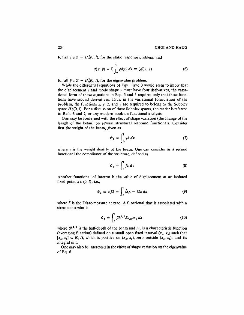
Consider the beam of Fig. I, with clamped supports and variable cross- sectional area h E C1[O, 4.' It is presumed that all dimensions of the cross section vary with the same ratio, so the moment of inertia of the cross- sectional area is I ( x ) = ah2(x), where a is a positive constant that depends on the shape of the cross section. The boundary-value problem, in operator form, is given as
where E is Young's modulus, h(x) 2 ho > 0, and f E C1[O, [I is distributed load.
For vibration, the formal operator eigenvalue equation is
where [ = w2, w is natural frequency, and p is material density. These boundary-value problems may be written in an equivalent .variational
form, essentially the principle of virtual work, by multiplying Eqs. 1 and 3 by arbitrary virtual displacements Z and j that satisfy the boundary condi- tions of Eqs. 2 and 4 and integrating by parts to obtain the variational equa- tions
Fi. 1 Clamped beam of variable cross-section area h(x).
'C1(n) denotes the wllection of i-times, wntinuously differentiable functions defined on a domain n.
Dow
nloa
ded
By:
[Uni
vers
ity o
f Iow
a Li
brar
ies]
At:
02:2
4 3
Febr
uary
200
8
234 CHOI AND HAUG
for all Z E Z = Hi(0, I), for the static response problem, and
for all g E Z = Hi(0, I), for the eigenvalue problem. While the differential equations of Eqs. 1 and 3 would seem to imply that
the displacement z and mode shape y must have four derivatives, the varia- tional form of these equations in Eqs. 5 and 6 requires only that these func- tions have second derivatives. Thus, in the variational formulation of the problem, the functions z, y, 5, and J are required to belong to the Sobolev space Hi(0, I). For a discussion of these Sobolev spaces, the reader is referred to Refs. 6 and 7, or any modern book on functional analysis.
One may be concerned with the effect of shape variation (the change of the length of the beam) on several structural response functionals. Consider first the weight of the beam, given as
where y is the weight density of the beam. One can consider as a second functional the compliance of the structure, defined as
Another functional of interest is the value of displacement at an isolated fixed point x E (0, I); i.e.,
where 8 is the Dirac-measure at zero. A functional that is associated with a stress constraint is
where Bh'I2 is the half-depth of the beam and m, is a characteristic function (averaging function) defined on a small open fixed interval (x,, x,) such that [x,, x,] c (0, I), which is positive on (x,, x,), zero outside (x,, x,), and its integral is 1.
One may also be interested in the effect of shape variation on the eigenvalue of Eq. 6.
Dow
nloa
ded
By:
[Uni
vers
ity o
f Iow
a Li
brar
ies]
At:
02:2
4 3
Febr
uary
200
8
SHAPE DESIGN SENSITIVITY ANALYSIS 235
B. Membrane
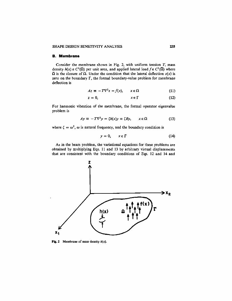
Consider the membrane shown in Fig. 2, with uniform tension T, mass density h(x) E C'(0) per unit area, and applied lateral load f E C1(:Ti) where IT is the closure of R. Under the condition that the lateral deflection z(x) is zero on the boundary T, the formal boundary-value problem for membrane deflection is
For harmonic vibration of the membrane, the formal operator eigenvalue problem is
Ay = - TV2y = (h(x)y = (By, x E R (13)
where ( = wZ, w is natural frequency, and the boundary condition is
As in the beam problem, the variational equations for these problems are obtained by multiplying Eqs. 11 and 13 by arbitrary virtual displacements that are consistent with the boundary conditions of Eqs. 12 and 14 and
Fig. 2 Membrane of mass density h(x).
Dow
nloa
ded
By:
[Uni
vers
ity o
f Iow
a Li
brar
ies]
At:
02:2
4 3
Febr
uary
200
8
236 CHOI AND HAUG
integrating by parts, to obtain
for all i E Z = HA(R), for the static response problem, and
for all j E Z = Hh(R), for the eigenvalue problem. As in the beam problem, while z and y would appear to require at least
two derivatives to be the solution of Eqs. 11 and 13, respectively, the gener- alized solution of the variational equations of Eqs. 15 and 16 require that z, y, Z, and 7 have only first-order derivatives; i.e., they must be in the Sobolev space HA@).
As in the beam problem, one can consider the effect of shape variation on the area of the membrane,
One can consider, as a second functional, the strain energy of the membrane
From Eq. 15, one notes that the strain energy $, is equal to half of the com- pliance
Also one can consider the effect of shape variation on the eigenvalue of Eq. 16.
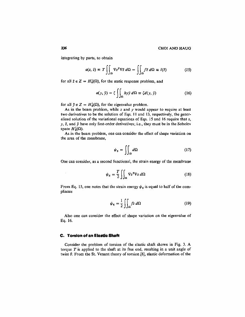
C. Torsion of an Elestlc Shaft
Consider the problem of torsion of the elastic shaft shown in Fig. 3. A torque T is applied to the shaft at its free end, resulting in a unit angle of twist 8. From the St. Venant theory of torsion [8], elastic deformation of the
Dow
nloa
ded
By:
[Uni
vers
ity o
f Iow
a Li
brar
ies]
At:
02:2
4 3
Febr
uary
200
8
SHAPE DESIGN SENSITIVITY ANALYSIS
Fig. 3 Torsion of an elastic shaft.
system is governed by the formal boundary-value problem
where z is the Prandtl stress function. The torque-angular deflection relation is given by T = GJB, where G is the shear modulus of the shaft material and J is torsional rigidity, given by [a]
Comparing Eqs. 11 and 20, one notes that they are exactly the same if f/T = 2. Hence the variational equation for the shaft is
for all i E Z = H1(S1). One can consider the torsional rigidity in Eq. 22 as a response functional,
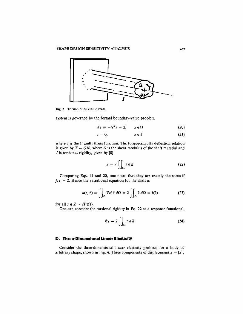
D. ThreaDimensional Linear Elasticity
Consider the three-dimensional linear elasticity problem for a body of arbitrary shape, shown in Fig. 4. Three components of displacement z = [z',
Dow
nloa
ded
By:
[Uni
vers
ity o
f Iow
a Li
brar
ies]
At:
02:2
4 3
Febr
uary
200
8
CHOI AND HAUG
Fig. 4 Three-dimensional elastic solid.
z2, z3IT characterize the displacement at each point in the elastic body. The strain tensor is defined as
where a subscript i denotes derivative with respect to x,. The stress-strain relation (generalized Hooke's law) is given as [8]
where D is the elastic modulus tensor, satisfying Dil" =, DJ"' and D'"' = DiJ", i, j, k, I = 1, 2, 3. The equilibrium equations are [8]
with boundary conditions
z' = 0, i = 1,2, 3, x E r0 (28) 3
~" ' (z ) = 2 ui'(z)nI = Ti, i = 1,2,3, x E r2 1-1
(29)
and boundary segment T1 is traction free, where n1 is the jth component of
Dow
nloa
ded
By:
[Uni
vers
ity o
f Iow
a Li
brar
ies]
At:
02:2
4 3
Febr
uary
200
8
SHAPE DESIGN SENSITIVITY ANALYSIS 239
the outward unit normal, F = [F', F', F3IT E [C1(@I3, and T = [Ti, T2, T3IT E [C10l3 .
The foregoing boundary-value problem may be reduced to variational form by multiplying both sides of Eq. 27 by an arbitrary displacement vector f = [fl, z2, p3IT that satisfies the boundary condition of Eqs. 28 and 29 and integrating by parts to obtain the variational equation
which must hold for all virtual displacements Z E Z, where Z is the space of kinematically admissible displacements; i.e.,
As a response functional, one can consider a mean stress over a tixed test volume R, such that II, c R,
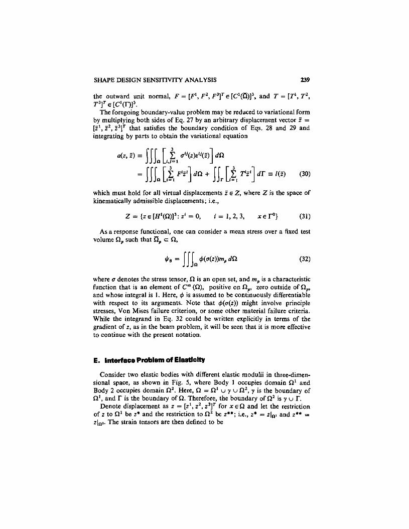
where a denotes the stress tensor, Q is an open set, and m, is a characteristic function that is an element of Cm (a), positive on Rp, zero outside of R,, and whose integral is 1. Here, 41 is assumed to be cont~nuously differentiable with respect to its arguments. Note that +(a(z)) might involve principle stresses, Von Mises failure criterion, or some other material failure criteria. While the integrand in Eq. 32 could be written explicitly in terms of the gradient of z, as in the beam problem, it will be seen that it is more effective to continue with the present notation.
E. Interface Problem of Elastlclty
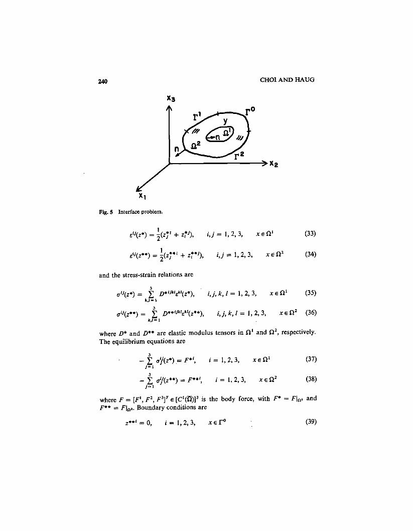
Consider two elastic bodies with different elastic moduli in three-dimen- sional space, as shown in Fig. 5, where Body 1 occupies domain R1 and Body 2 occupies domain RZ. Here, R = R1 u y u RZ, y is the boundary of R1, and r is the boundary of R. Therefore, the boundary of RZ is y u T.
Denote displacement as z = [zl, zz, z3IT for x E R and let the restriction of z to R1 be z* and the restriction to RZ be z**; i.e., z* = zl,, and z** = zln2. The strain tensors are then defined to be
Dow
nloa
ded
By:
[Uni
vers
ity o
f Iow
a Li
brar
ies]
At:
02:2
4 3
Febr
uary
200
8
CHOI AND HAUG
Fig. 5 Interface problem.
and the stress-strain relations are
where D* and D** are elastic modulus tensors in R' and R2, respectively. The equilibrium equations are
3 - C ~ $ j ( z * ) ,= F*', i = 1,2,3 , x E R1
j = 1
where F = [F', F Z , F3]' E [C1(TI)13 is the body force, with F* = FI,t and F** = FI,L Boundary conditions are
Dow
nloa
ded
By:
[Uni
vers
ity o
f Iow
a Li
brar
ies]
At:
02:2
4 3
Febr
uary
200
8
SHAPE DESIGN SENSITIVITY ANALYSIS 241
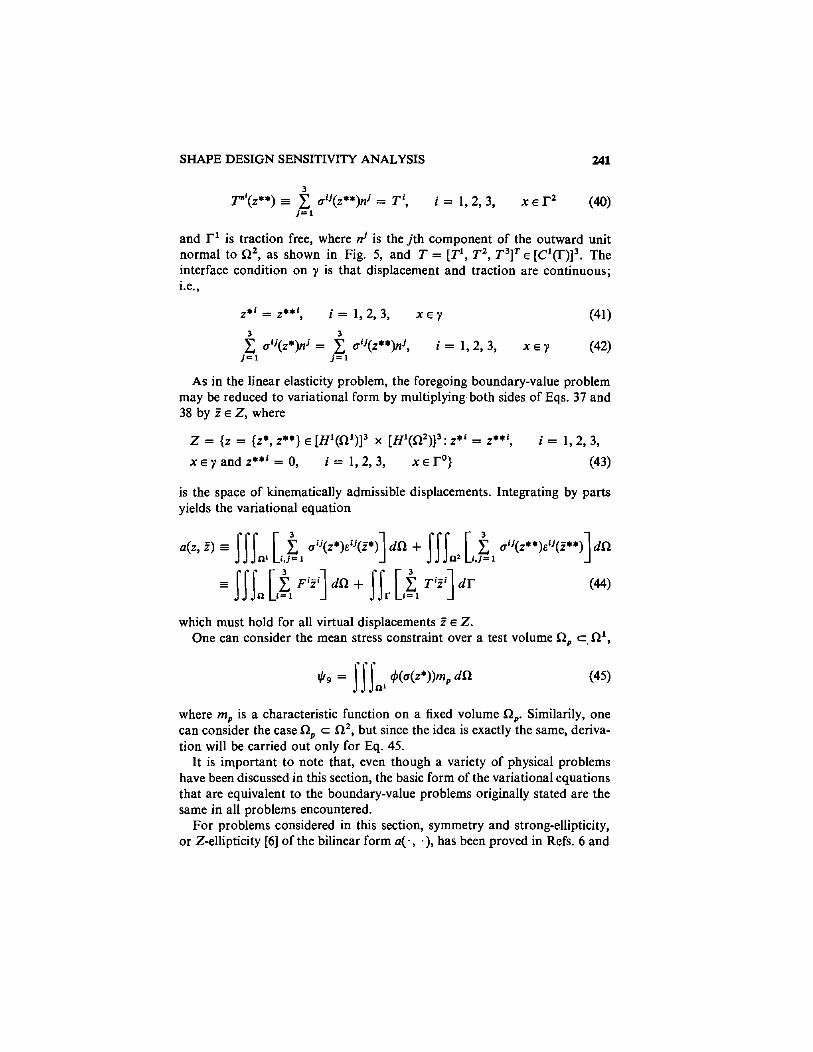
and r1 is traction free, where nj is the jth component of the outward unit normal to R2, as shown in Fig. 5, and T = [T1, T 2 , T3IT E [ C 1 Q I 3 . The interface condition on y is that displacement and traction are continuous; l.e.,
As in the linear elasticity problem, the foregoing boundary-value problem may be reduced to variational form by multiplyingboth sides of Eqs. 37 and 38 by f E Z, where
Z = {z = {z*, z**} E [H1(R1)I3 x [H1(R2)I3: = z**~ , i = l , 2 , 3 ,
x ~ y a n d z * * ' = O , i = 1 , 2 , 3 , x ~ l - ' ) (43)
is the space of kinematically admissible displacements. Integrating by parts yields the variational equation
Pii d + J [i ~ i , ] dl- - SSI. [f I r i = 1
which must hold for all virtual displacements 2 E Z. One can consider the mean stress constraint over a test volume R, c , R 1 ,
where m, is a characteristic function on a fixed volume R,. Similarily, one can consider the case R, c R2, but since the idea is exactly the same, deriva- tion will be carried out only for Eq. 45.
It is important to note that, even though a variety of physical problems have been discussed in this section, the basic form of the variational equations that are equivalent to the boundary-value problems originally stated are the same in all problems encountered.
For problems considered in this section, symmetry and strong-ellipticity, or Z-ellipticity [6] of the bilinear form a ( . , .), has been proved in Refs. 6 and
Dow
nloa
ded
By:
[Uni
vers
ity o
f Iow
a Li
brar
ies]
At:
02:2
4 3
Febr
uary
200
8
242 CHOI AND HAUG
9 and existence and uniqueness of the solution of the variational equation follows from the Lax-Milgram theorem [6], if the right side of the variational equation is a bounded linear functional of P in the Sobolev norm.
The importance of the variational formulation of problems of linear mechanics will further be seen in treating shape design sensitivity analysis in subsequent sections. The variational formulation of prototype problems discussed in this section serves as the principal tool in development of a broadly applicable and rigorous design sensitivity analysis method.
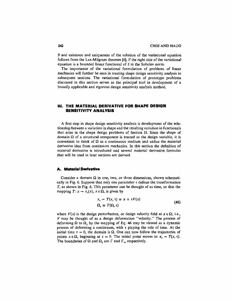
Ill. THE MATERIAL DERIVATIVE FOR SHAPE DESIQN SENSITIVITY ANALYSIS
A first step in shape design sensitivity analysis is development of the rela- tionship between a variation in shape and the resulting variation in functionals that arise in the shape design problems of Section 11. Since the shape of domain R of a structural component is treated as the design variable, it is convenient to think of R as a continuous medium and utilize the material derivative idea from continuum mechanics. In this section the definition of material derivative is introduced and several material derivative formulas that will be used in later sections are derived.
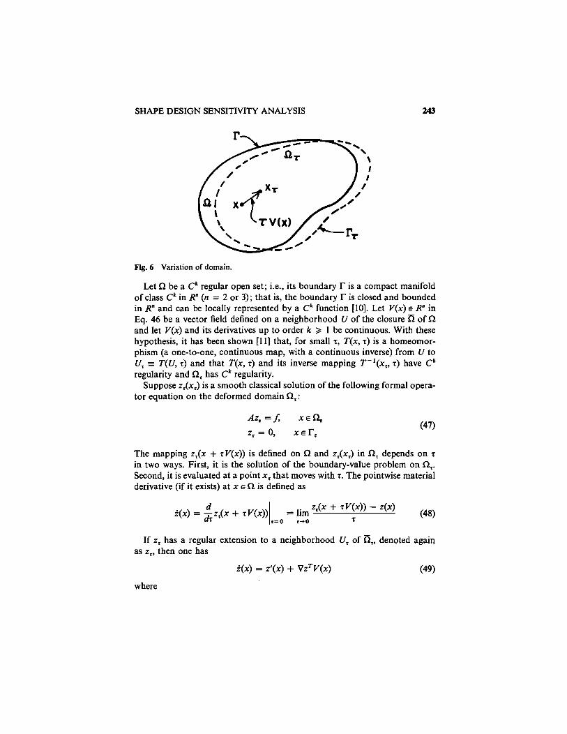
Consider a domain R in one, two, or three dimensions, shown schemati- cally in Fig. 6. Suppose that only one parameter r defines the transformation T, as shown in Fig. 6. This parameter can be thought of as time, so that the mapping T : x -t x,(x), x E R, is given by
where V(x) is the design perturbation, or design velocity field at x E R; i.e., Y may be thought of as a design deformation "velocity." The process of deforming R to R, by the mapping of Eq. 46 may be viewed as a dynamic process of deforming a continuum, with r playing the role of time. At the initial time r = 0, the domain is R. One can now follow the trajectories of points x E R, beginning at r = 0. The initial point moves to x , = T(x, T). The boundaries of R and a, are l- and T,, respectively.
Dow
nloa
ded
By:
[Uni
vers
ity o
f Iow
a Li
brar
ies]
At:
02:2
4 3
Febr
uary
200
8
SHAPE DESIGN SENSITIVITY ANALYSIS
Fig. 6 Variation of domain.
Let R be a Ck regular open set; i.e., its boundary l- is a compact manifold of class Ck in Rn (n = 2 or 3); that is, the boundary r is closed and bounded in R" and can be locally represented by a Ck function [lo]. Let V(x) s R" in Eq. 46 be a vector field defined on a neighborhood U of the closure a of R and let V(x) and its derivatives up to order k 3 1 be continuous. With these hypothesis, it has been shown [I 11 that, for small T, T(x, T) is a homeomor- phism (a one-to-one, continuous map, with a continuous inverse:) from U to U f = T(U, T) and that T(x, T) and its inverse mapping T-'(x,, T) have Ck regularity and R, has Ck regularity.
Suppose z,(x,) is a smooth classical solution of the following formal opera- tor equation on the deformed domain R,:
The mapping z,(x + zV(x)) is defined on R and z,(x,) in R, depends on T
in two ways. First, it is the solution of the boundary-value problem on R,. Second, it is evaluated at a point x, that moves with T. The pointwise material derivative (if it exists) at x E R is defined as
d z.(x + TV(X)) - z(x) i(x) = -z,(x + zV(x)) = lim
& r=O r-o T - (48)
If z, has a regular extension to a neighborhood U, of a,, denoted again as z,, then one has
where
Dow
nloa
ded
By:
[Uni
vers
ity o
f Iow
a Li
brar
ies]
At:
02:2
4 3
Febr
uary
200
8
CHOI AND HAUG
is the partial derivative of z. One attractive feature of the partial derivative is that, with smoothness assumptions, it commutes with the derivative with respect to independent variables; i.e.,
If z,(x,) is the solution of the following variational equation on the de- formed domain R,:
for all 2, E Z,, where Z, c Hm(RJ is the space of kinematically admissible displacements on R,, then z, E Z , c Hm(R,). For z, E Hm(R,), the material derivative i (if it exists) at R is defined as
Note that for z, E Hm(R,), the pointwise derivative of Eq. 48 is meaningless. It is shown in Ref. 11 that, since T(x, T) is a Ck homeomorphism, the Sobolev space Hm(R), for rn < k, is preserved by T(x, T); i.e.,
This fact is used in Ref. 12 to prove existence of the material derivative i in problems treated in Section 11.
For z, E Hm(R,), it is shown in Ref. 6 that for a Ck regular open set R,, for k large enough, there exists an extension of z, in a neighborhood U, of 0, and hence one has the partial derivative z', as in Eq. 50. In this case the equality in Eq. 50 must be interpreted in tbe Hm(R) norm, as in Eq. 53.
B. Material Derivative Formulas
The following lemmas, which give the material derivatives of several func- tional~, are proved in Ref. 12.
Lemma I: Let $, be a domain functional, defined as an integral over R,,
Dow
nloa
ded
By:
[Uni
vers
ity o
f Iow
a Li
brar
ies]
At:
02:2
4 3
Febr
uary
200
8
SHAPE DESIGN SENSITIVITY ANALYSIS 245
where f, is a regular function defined on R,. If R has Ck regularity, then the material derivative of $, at R is
It is interesting and important to note that it is only the normal component (VTn) of the boundary design velocity appearing in Eq. 55 that is of impor- tance in accounting for the effect of domain variation. In fact, it is shown in Ref. 11 that if a general domain functional $ has a gradient at R and 0 has Ck+' regularity, then one can consider only the normal component (VTn) of the design velocity field on the boundary for the derivative calculations. The basic idea behind this result is that T,(VT) = T for all s, where VT is the component of the velocity field V of Eq. 46 that is tangent to the boundary T. That is, the tangential component VT of the velocity field does not deform the domain R.
Next consider a functional defined as an integration over T,,
where g, is a regular function defined on T,.
Lemma 2: Suppose g, in Eq. 56 is a regular function defined on r, and the mapping V + g is linear and continuous. If R has Cktl regularity, the material derivative of I, in Eq. 56 at R is
where H is the curvature of the boundary T in R2 and twice the mean cur- vature of T in R3.
The choice of n as directed outward from the domain R defines the orienta- tion of the boundary T. If one changes the orientation of T, then n is changed to - n and one must change H to - H.
Finally, consider a special functional defined as an integration over T, as
Dow
nloa
ded
By:
[Uni
vers
ity o
f Iow
a Li
brar
ies]
At:
02:2
4 3
Febr
uary
200
8
246 CHOI AND HAUG
where h, is a regular field defined on T, and hence hTn, is a regular function on rr.
Lemma 3: Suppose h, in Eq. 58 is a regular field defined on T, and the mapping V + h is linear and continuous. If R has Ck+' regularity, then the material derivative of in Eq. 58 at R is
$; = 1 [hl(x)'n + div h(VTn)] dT r
(59)
IV. ADJOINT VARIABLE METHOD OF SHAPE DESIGN SENSITIVITY ANALYSIS
As seen in Section 111, the static response of a structure depends on the shape of the domain. Existence of material derivative i, which is proved in Refs. 12 and 13, is used in this section to derive an adjoint variable method for design sensitivity analysis of general functionals, utilizing the material derivative formulas of Section 111. An adjoint problem that is closely related to the original structural problem is defined and explicit formulas for shape design sensitivity are obtained.
A. Dlfferentlablllty of Bilinear Forms and Static Response
Basic design differentiability results for energy bilinear forms and static response are proved in Ref. 12 for the problems treated in Section 11. These differentiability results are used here to develop shape design sensitivity formulas that are applicable to the beam, membrane, and torsion problems of Section 11. Shape design sensitivity formulas for the linear elasticity prob- lems will be considered separately.
The variational equations of the problems of Section 11, on a deformed domain, are of the form
for all 2, E Z,, where 2; c Hm(RJ is the space of kinematically admissible displacements and c(., .) is a bilinear mapping that can be obtained from the integrand of the variational equation. It is shown in Ref. 12 that the load
Dow
nloa
ded
By:
[Uni
vers
ity o
f Iow
a Li
brar
ies]
At:
02:2
4 3
Febr
uary
200
8
SHAPE DESIGN SENSITIVITY ANALYSIS 247
linear forms I&) for the problems of Section I1 are also differentiable with respect to design.
A substantially more powerful result from Ref. 12 is that the solution of Eq. 60 is differentiable with respect to design; i.e., the material derivative i defined in Eq. 53 exists. Note that the material derivative i depends on the direction of the velocity field. It is shown in Ref. 12 that i is linear in V and in fact is the Frkchet derivative with respect to design, evaluated in the direction V. This linearity and continuity of the mapping V + i justify use of only the normal component (VTn) of the velocity field V in the derivation of material derivatives, as in Eqs. 57 and 59.
Taking the material derivative of both sides of Eq. 60, using Eq. 55, and noting that the partial derivatives with respect to s and x commute with each other, one has
[a(z, P)]' = al(z, 2) + a ( i , Z ) = I'(P) (61)
for all Z E 2, where
[a(z, Z)]' = Isn [c(zl, Z ) + c(z, I ) ] d R + c(z, Z)(VTn) d r 1 = JJ. [c(i - VzTV, Z ) + c(z, 2 - VPTV)] d R
and
The fact that the partial derivatives of the coe%cients, which depend on cross-sectional area and thickness, in the bilinear mapping c ( . , .) are zero has been used in Eq. 62 and f' = 0 has been used in Eq. 63, because they do not depend explicitly on r. For Z,, one can take Z,(x + rV(x)) = 9(x); i.e., choose Z as constant on the line x, = x + rV(x). Then if P is an arbitrary element of Hm(R) that satisfies kinematic boundary conditions on I-, 9, is an arbitrary element of Hm(R,) that satisfies kinematic boundary conclitions on r , . In this case, using Eq. 49, one has
Dow
nloa
ded
By:
[Uni
vers
ity o
f Iow
a Li
brar
ies]
At:
02:2
4 3
Febr
uary
200
8
248 CHOI AND HAUG
and from Eqs. 61, 62, and 63, one obtains, using Eq. 64,
and
Then, Eq. 61 can be rewritten to provide the result
a(& Z) = lr(E) - al(z, 2)
[c(VzTV, f ) + C(Z, Vf - f (VfT V)] dR
for all f E Z. Note that if the state z is known as the solution of Eq. 60 at Q and if V
is known, Eq. 67 is a variational equation with the same energy bilinear form for i E Hm(R), which satisfies kinematic boundary conditions. Indeed, for second-order problems (membrane, shaft, elasticity), kinematic boundary conditions are only assigned to z, so if z, = 0 on T,, i = 0 on T and i satisfies kinematic boundary conditions. For higher order problems such as the beam and plate, one can show that 2 also satisfies kinematic boundary conditions [12].
Note that the right side of Eq. 67 is linear in f and that the energy bilinear form on the left is Z-elliptic. Thus, Eq. 67 has a unique solution i [6]. The fact that there is a unique solution of Eq. 67 agrees with the previously stated result that the shape design derivative of the solution of the state equation exists.
B. Aaolnt Variable Deslgn Sensltlvlty Analysis
Consider a general functional that may be written in integral form as
where z E H1(Q), VZ = [z,, z2, zJT, and the function g is continuously
Dow
nloa
ded
By:
[Uni
vers
ity o
f Iow
a Li
brar
ies]
At:
02:2
4 3
Febr
uary
200
8
SHAPE DESIGN SENSITIVITY ANALYSIS 249
differentiable with respect to its arguments. In case z E H2(R), second deriva- tives of z may appear in the integrand of Eq. 68. This case will be treated as specific applications arise. Note that JI depends on R, in two ways. First, there is the obvious dependence of the integral on its domain of integration. Second, the state z, depends'on the domain R,, through the variational equa- tion of Eq. 60.
Taking the variation of the functional of Eq. 68, using the material deriva- tive formula of Eq. 51 and Eq. 55, one has
where g,, = [agpz, , aglaz,, ag/az,]. Using Eq. 49, Eq. 69 can be rewritten as
Note that i and V i depend on the design velocity field V. The objective is to obtain an explicit expression of JI' in terms of the velocity field V, which requires rewriting the first two terms of the first integral on the right of Eq. 70 explicitly in terms of V.
An adjoint equation is introduced by replacing i in Eq. 70 by a virtual displacement X and equating terms involving to the energy bilinear form in I and X, yielding the adjoint equation for the adjoint variable I,
which must hold for all 1 E Z. A simple application of the Schwartz: inequality to the right of Eq. 71 shows that it is a bounded linear functional of in the H1(R) norm. Thus, the Lax-Milgram Theorem [6] guarantees that Eq. 71 has a unique solution I, which is called the adjoint variable associated with the constraint of Eq. 68.
To take advantage of the adjoint equation, one may evaluate Eq. 71 at X = 2, since i E 2, to obtain the expression
Similarly, one may evaluate the identity of Eq. 67 at 2 = I, since both are
Dow
nloa
ded
By:
[Uni
vers
ity o
f Iow
a Li
brar
ies]
At:
02:2
4 3
Febr
uary
200
8
250 CHOI AND HAUG
in 2, to obtain
Recalling that the energy bilinear form a ( . , .) is symmetric in its arguments, the left sides of Eqs. 72 and 73 are equal, yielding
Using Eqs. 67 and 74, Eq. 70 yields the desired result,
where the integral over $2 can be transformed to a boundary integral by integrating by parts and using the formal operator equation. This will be done for each type of structural component encountered. The fact that one can express the design sensitivity I' as a boundary integral gives significant advantages in numerical calculations.
Note that evaluation of the design sensitivity formula of Eq. 75 requires solution of the variational equation of Eq. 60 for z. Similarly, the variational adjoint equation of Eq. 71 must be solved for the adjoint variable I. This is an efficient calculation, using finite element analy;is, if the boundary-value problem for z has already been solved, requiring only evaluation of the solu- tion of the same set of finite element equations with a different right side (the adjoint load).
C. Analytical Examples of Static Design Sensitlvsty Analysis
The beam, membrane, and torsion problems of Section I1 are used here as examples with which to calculate design sensitivity formulas, using the adjoint variable method. The linear elasticity problem will be considered in the next subsection.
1. Beam. Consider the clamped beam of Section I1 with $2 = (0, [) c R1 and I = ah2. Consider first the weight of the beam, given in Eq. 7 . Taking the
Dow
nloa
ded
By:
[Uni
vers
ity o
f Iow
a Li
brar
ies]
At:
02:2
4 3
Febr
uary
200
8
SHAPE DESIGN SENSITIVITY ANALYSIS 251
variation of Eq. 7, using Eq. 55 with (yh)' = 0, one obtains
where V(0) and V(l) are perturbations of end point locations for the beam, taken as positive if V(0) and V(1) cause the end points to move in the positive x-direction. Note that this direct variation gives the explicit form of variation of structural weight in terms of variation of shape. Thus, no adjoint problem needs to be defined.
Consider as a second functional the compliance of the beam in Eq. 8. Note that the integrand of Eq. 8 depends on the load f. However, since f' = 0, one can treat Eq. 8 as the functional form of Eq. 68. Hence, the adjoint equation of Eq. 71 is
for all 1 E Z. Since the load functional on the right of Eq. 77 is precisely the same as the load functional for the original beam problem of Eq. 5, in this special case I = z and from Eq. 75, one obtains
Integrating the first term of the integral in Eq. 78 by parts, one obtains
For a clamped beam, using Eqs. 1 and 2, Eq. 79 becomes
As noted, the design sensitivity in Eq. 80 is expressed as a boundaly evalua- tion'and is given explicitly in terms of movement of the boundary.
Consider next a functional in Eq. 9 that defines the value of displacement at an isolated fixed point 2 E (0, I). Since 8(x - 2) is defined on a neighborhood of [0, I] by zero extension and 2 is a fixed point, bl(x - 2) = 0. Thus, one can treat Eq. 9 as the functional form of Eq. 68 and the adjoint equation is, from Eq. 71,
Dow
nloa
ded
By:
[Uni
vers
ity o
f Iow
a Li
brar
ies]
At:
02:2
4 3
Febr
uary
200
8
CHOI AND HAUG
for all 1 E Z. By the Sobolev imbedding theorem [q, the functional on the right side of Eq. 81 is bounded and linear in 1 and Eq. 81 has a unique solu- tion 1. Note that I is the displacement due to a unit load at 2. That is, with smoothness assumptions, the variational equation of Eq. 81 is equivalent to the formal operator equation
From Eq. 75, one obtains
Integrating the first two terms of the integral in Eq. 84 by parts, one obtains
For a clamped beam, using Eqs. 1, 2, 82, and 83, Eq. 85 becomes simply
Consider another functional in Eq. 10 that is associated with a stress constraint. Assume that one is interested in the averaged stress on the fixed interval (x,, x,); i.e., m, in Eq. 10 does not change with T. One can extend m, on R1 by extending it to zero value outside (0, I), so m, = 0.
Taking the variation of Eq. 10, using Eqs. 51 and 55, one has
Dow
nloa
ded
By:
[Uni
vers
ity o
f Iow
a Li
brar
ies]
At:
02:2
4 3
Febr
uary
200
8
SHAPE DESIGN SENSITIVITY ANALYSIS 253
since mp(0) = mp(l) = 0 . As in the general derivation of the adjoint equation of Eq. 71, one may define the adjoint equation by replacing i in the first term on the right side of Eq. 87 by 1, to define a load functional for the adjoint equation, obtaining
for all X E 2. In the Sobolev space H2(0, I), the functional on the right side of Eq. 88 is a bounded linear functional. Thus, by the Lax-Milgram Theorem [6], Eq. 88 has a unique solution I .
With smoothness assumptions, the variational equation of Eq. 88 is equiva- lent to the formal operator equation
Since i E 2, one may evaluate Eq. 88 at 1 = i to obtain
Similarly, one may evaluate the identity of Eq. 67 at Z = I , since both are in 2, to obtain
~ ( 2 , I ) = I ~ ( I ~ - at(z9 A) (92)
Since the energy bilinear form a ( . , .) is symmetric, Eqs. 87, 91, and 92 yield
which can be rewritten, using Eq. 67, as
Integrating the first two terms and the fourth term in the integral by parts, Eq. 94 becomes
Dow
nloa
ded
By:
[Uni
vers
ity o
f Iow
a Li
brar
ies]
At:
02:2
4 3
Febr
uary
200
8
254 CHOI AND HAUG
For a clamped beam, using Eqs. 1, 2, 89, and 90, Eq. 95 becomes simply
2. Membrane. Consider the membrane of Section I1 with mass density h. The area of the membrane is given in Eq. 17. Taking variation of Eq. 17, using Eq. 55, one has
Note that this direct variation calculation gives the explicit form of variation of area in terms of the normal movement (vTn) of the boundary. Thus, for this functional, no adjoint problem needs to be defined.
Consider as a second functional the strain energy of the membrane in Eq. 19. Note that the integrand of Eq. 19 depends on the loadf. However, since f' = 0, one can treat Eq. 19 as the functional form of Eq. 68. Hence, the adjoint equation of Eq. 71 is
for all 1 E Z. Note that the load functional on the right of Eq. 98 is precisely half the load functional for the original membrane problem of Eq. 15. Hence, in this special case, I = 1/22 and from Eq. 75, using z = 0 on T, one has
Integrating the first term of the domain integral in Eq. 99 by parts, one obtains
Dow
nloa
ded
By:
[Uni
vers
ity o
f Iow
a Li
brar
ies]
At:
02:2
4 3
Febr
uary
200
8
SHAPE DESIGN SENSITIVITY ANALYSIS 255
Since z = 0 on T, Vz = (VzTn)n on r. Hence, using Eq. 11, the domain integral in Eq. 100 is zero and one has the simplified result
As noted, the design sensitivity in Eq. 101 is expressed as a boundary integral and only the normal movement (VTn) of the boundary appears.
3. Torsion of an Elastic Shaft. Consider torsion of the elastic shaft of Section 11. One can consider the torsional rigidity in Eq. 24 as a response functional. The adjoint equation is, from Eq. 71,
for all 1 E 2. Thus, in this special case 1 = z. Comparing this with the membrane problem, one obtains
D. Elastlclty Problems
Shape design sensitivity analysis of the three-dimensional elasticity and interface problems of Section I1 is carried out here, using the adjoint variable method.
1. Three-Dimensional Elasticity. Consider the three-dimensional elasticity problem of Section I1 with a mean stress constraint over a test volume R, c R, as in Eq. 32. For boundary perturbation in the elasticity problem, it is supposed that the boundary T = To u T' u TZ is varied, except that the curve aT2 that bounds the loaded boundary surface TZ is fixed, so the velocity field Va t dT2 is zero. There are two kinds of boundary loads that may be considered. One is a conservative loading that depends on the position, but not the shape of the boundary. The other is a more general nonconservative load that depends not only on the position, but also on the shape of the boundary.
Consider first the elementary conservative loading case in which the trac- tion Ti in Eq. 29 depends on position only. Taking the variation of Eq. 30, using Eqs. 51, 55, and 57 and the fact that Fi' = 0, one obtains
Dow
nloa
ded
By:
[Uni
vers
ity o
f Iow
a Li
brar
ies]
At:
02:2
4 3
Febr
uary
200
8
256 CHOI AND HAUG
for all i E Z. Using Eqs. 49 and 64, Eq. I04 can be rewritten as
for all Z E Z. As in Eq. 67, Eq. 105 is a variational equation for i E Z. Taking the variation of the functional of Eq. 32, using material derivative
formulas of Eqs. 49 and 55 and mb = 0, one obtains
because m, = 0 on I'. As in the general derivation of Eq. 71, one may replace the variation in
state i by a virtual displacement 1 in the first term on the right side of Eq. 106 to define a load functional for the adjoint equation, obtaining as in Eq. 71,
for all X E Z. One may directly show that the linear form in 1 on the right
Dow
nloa
ded
By:
[Uni
vers
ity o
f Iow
a Li
brar
ies]
At:
02:2
4 3
Febr
uary
200
8
SHAPE DESIGN SENSITIVITY ANALYSIS 257
side of Eq. 107 is bounded in [H1(n)13, so Eq. 107 has a unique solution for a displacement field I, with the right side of Eq. 107 defining the adjoint load functional (virtual work associated with a virtual displacement A).
With smoothness assumptions, Eq. 107 is equivalent to the formal opera- tor equation
with boundary conditions
Since i E Z, one may evaluate Eq. 107 at 1 = z to obtain
Similarly, since P E Z and I E Z, one may evaluate Eq. 105 at i? = I to obtain
By the Betti reciprocal theorem [8],
for all z and i E [H1(Q)l3. Thus, a(i, I) = a(I, i) and Eqs. 106, 110, and 11 1 yield
Dow
nloa
ded
By:
[Uni
vers
ity o
f Iow
a Li
brar
ies]
At:
02:2
4 3
Febr
uary
200
8
258 CHOI AND HAUG
As before, integrating the first and last integrals by parts, using Eqs. 27, 29, 108, and 109 and the fact m, = 0 on T, one has
On To, z = I = 0 implies V z i = (vr iTn)n and V I i = (vziTn)n. Hence, Eq. 114 becomes
which is the desired result. Next, consider the more general nonconservative loading case. For ex-
ample, in pressure loading, traction is given as
Substituting T' into Eq. 30 and taking the variation of both sides, using Eqs. 51, 55, and 59 and the factp' = 0 and F" = 0, one has
Dow
nloa
ded
By:
[Uni
vers
ity o
f Iow
a Li
brar
ies]
At:
02:2
4 3
Febr
uary
200
8
SHAPE DESIGN SENSInVITY ANALYSIS 259
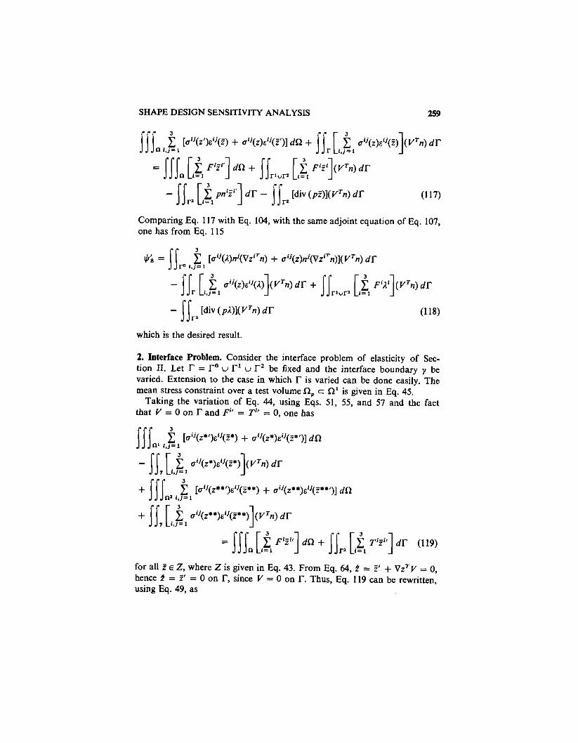
Comparing Eq. 117 with Eq. 104, with the same adjoint equation of Eq. 107, one has from Eq. 1 15
which is the desired result.
2. Interface Problem. Consider the interface problem of elasticity of Sec- tion 11. Let r = r0 u r1 u r2 be fixed and the interface boundary y be varied. Extension to the case in which l- is varied can be done easily. The mean stress constraint over a test volume R, c R1 is given in Eq. 45.
Taking the variation of Eq. 44, using Eqs. 51, 55, and 57 and the fact that V = 0 on r and Fi' = Ti' = 0, one has
C C C 9
for all P E 2, where Z is given in Eq. 43. From Eq. 64, k = Z' + V z T v = 0, hence I = Z' = 0 on r, since V = 0 on r. Thus, Eq. 119 can be rewritten, using Eq. 49, as
Dow
nloa
ded
By:
[Uni
vers
ity o
f Iow
a Li
brar
ies]
At:
02:2
4 3
Febr
uary
200
8
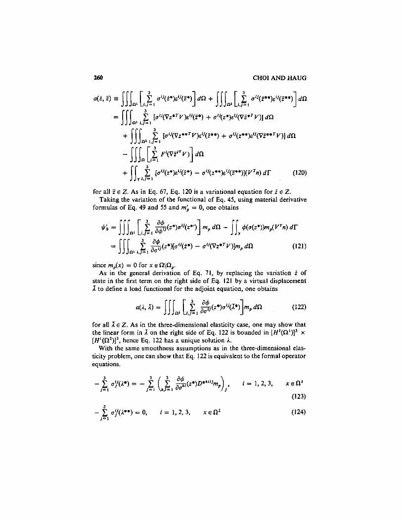
260 CHOI AND HAUG
for all f E 2. As in Eq. 67, Eq. 120 is a variational equation for i E 2. Taking the variation of the functional of Eq. 45, using material derivative
formulas of Eq. 49 and 55 and mb = 0, one obtains
since mp(x) = 0 for x E R\Rp. As in the general derivation of Eq. 71, by replacing the variation i of
state in the first term on the right side of Eq. 121 by a virtual displacement to define a load functional for the adjoint equation, one obtains
for all 2 E 2. As in the three-dimensional elasticity case, one may show that the linear form in 2 on the right side of Eq. 122 is bounded in [H' (Q' ) ]~ x [ H ' ( R ~ ) ] ~ , hence Eq. 122 has a unique solution I.
With the same smoothness assumptions as in the three-dimensional elas- ticity problem, one canshow that Eq. 122 is equivalent to the formal operator equations.
Dow
nloa
ded
By:
[Uni
vers
ity o
f Iow
a Li
brar
ies]
At:
02:2
4 3
Febr
uary
200
8
SHAPE DESIGN SENSITIVITY ANALYSIS 261
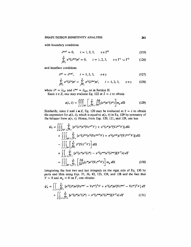
with boundary conditions
and interface conditions
where I* = I[,, and I** = A~,Z, as in Section 11. Since i E 2, one may evaluate Eq. 122 at 1 = i to obtain
Similarily, since Z and I Z, Eq. 120 may be evaluated at 2 = I to obtain the expression for a(i, I), which is equal to a(I, i ) in Eq. 129 by symmetry of the bilinear form a(v, v) . Hence, from Eqs. 120, 121, and 129, one has
Integrating the first two and last integrals on the right side of Eq. 130 by parts and then using Eqs. 37, 38, 42, 123, 124, and 128 and the fact that V = 0 and m, = 0 on r, one obtains
Dow
nloa
ded
By:
[Uni
vers
ity o
f Iow
a Li
brar
ies]
At:
02:2
4 3
Febr
uary
200
8
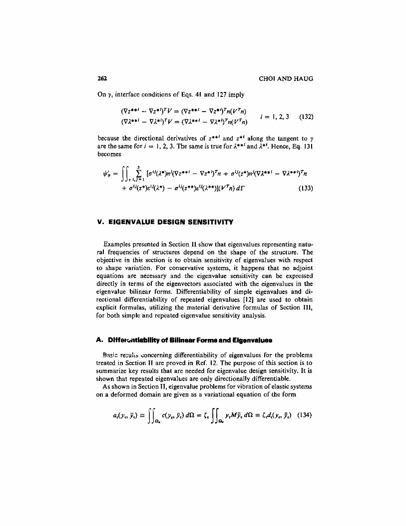
262 CHOI AND HAUG
On y, interface conditions of Eqs. 41 and 127 imply
because the directional derivatives of z**' and z*' along the tangent to y are the same for i = 1, 2, 3. The same is true for A**' and A*'. Hence, Eq. 131 becomes
V. EIGENVALUE DESIGN SENSITIVITY
Examples presented in Section I1 show that eigenvalues representing natu- ral frequencies of structures depend on the shape of the structure. The objective in this section is to obtain sensitivity of eigenvalues with respect to shape variation. For conservative systems, it happens that no adjoint equations are necessary and the eigenvalue sensitivity can be expressed directly in terms of the eigenvectors associated with the eigenvalues in the eigenvalue bilinear forms. Differentiability of simple eigenvalues and di- rectional differentiability of repeated eigenvalues [12] are used to obtain explicit formulas, utilizing the material derivative formulas of Section 111, for both simple and repeated eigenvalue sensitivity analysis.
A. Diffeffintiablllty of Bilinear Forms and Eigenvalues
Bask. re~u:is concerning differentiability of eigenvalues for the problems treated in Section I1 are proved in Ref. 12. The purpose of this section is to summarize key results that are needed for eigenvalue design sensitivity. It is shown that repeated eigenvalues are only directionally differentiable.
As shown in Section 11, eigenvalue problems for vibration of elastic systems on a deformed domain are given as a variational equation of the form
Dow
nloa
ded
By:
[Uni
vers
ity o
f Iow
a Li
brar
ies]
At:
02:2
4 3
Febr
uary
200
8
SHAPE DESIGN SENSITIVITY ANALYSIS 263
for all 8, E Z,, where Z, c Hm(RJ is the space of kinematically admissible displacements and c ( . , .) is a bilinear mapping. Since Eq. 134 is homogene- ous in y,, a normalizing condition must be given to have unique eigenfunc- tions. The normalizing condition is
The energy bilinear form on the left side of Eq. 134 is the same as the bilinear form in the static problems treated in Section 111. Therefore, it has the same differentiability properties as discussed there. The bilinear form d, on the right side of Eq. 134 represents mass effects in vibration problems. In most cases, it is even more regular than the energy bilinear form in its dependence on design and eigenfunction.
1. Simple Eigenvalues. It is shown in Ref. 12 that a simple eigenvalue [ is differentiable. It is 'shown in Ref. 14 that the corresponding eigenfunction y is also differentiable. In fact, material derivatives of both the eigenvalue and eigenfunction are linear in V, hence they are Frkchet derivatives of the eigenvalue and eigenfunction. As in the static response case, Linearity and continuity of the mapping V -P j~ allows [I21 one to use only the normal component (VTn) of the design velocity field V in derivation of the material derivative, as in Eq. 55.
Taking the material derivative of both sides of Eq. 134, using Eq. 55 and noting that the partial derivatives with respect to T and x comnlute with each other, one has
for all 8 E Z, where
and
Dow
nloa
ded
By:
[Uni
vers
ity o
f Iow
a Li
brar
ies]
At:
02:2
4 3
Febr
uary
200
8
264 CHOI AND HAUG
As in Eq. 62, the fact that the partial derivatives of the coefficients in the bilinear mapping c ( . , .) are zero has been used in Eq. 137. Also, M' = 0 has been'used in Eq. 138. As in the static response case, for j , one can take j l (x + rV(x)) = j(x). Hence, if j E Z is arbitrary, then j , is an arbitrary element of Z,. Also, from Eq. 49, one has
and from Eqs. 135, 136, and 137 one obtains, using Eq. 138,
and
( y , ) = - j [ (VyTV)Mj + yM(VjTV)] + yMj(VTn) dl- (141) n I-
Since 7 E Z, one may evaluate Eq. 136 with j j = y, using symmetry of the bilinear forms, to obtain
Noting that j, E Z, one sees that the term in brackets on the right of Eq. 142 is zero. Furthermore, due to the normalizing condition of Eq. 135, one has the simplified equation
where, as in the static response case, the integral' over R can be transformed to a boundary integral by integrating by parts and using the formal operator equation. This will be done for each class of problems encountered.
Dow
nloa
ded
By:
[Uni
vers
ity o
f Iow
a Li
brar
ies]
At:
02:2
4 3
Febr
uary
200
8
SHAPE DESIGN SENSITIVITY ANALYSIS 265
Note that the directional derivative of the eigenvalue is linear in V, since variations of the bilinear forms on the right side of Eq. 143 are linear in V. It should be emphasized, however, that the validity of this result rests on existence of derivatives of eigenvalues and eigenfunctions.
2. Repeated Eigenvalues. Consider now the situation in which an eigenvalue ( has multiplicity m > 1 at 0; i.e.,
a , ) = d y i , ) for all j E Z i , j = 1 , 2 ,..., m (144)
d(yi, y') = 611
It is shown in Ref. 12 that the repeated eigenvalue [ is a continuous func- tion of design, but the corresponding eigenfunctions are not. Moreover, it is shown in Ref. 12 that at R, where the eigenvalue is repeated m times, the eigenvalue ( is only directionally differentiable and the directional derivatives (;(V) in the direction V are the eigenvalues of the m x m matrix A with elements
-U = a'(yi, y3 - Cd'(yi, y')
The notation ( ; ( V ) is used here to emphasize dependence of the directional derivative on V. As in the simple eigenvalue case, the integral over R in Eq. 145 can be transformed to a boundary integral by integrating by parts and using the formal operator equation. This will be done for each class of problem encountered.
If one changes the d-orthonormal basis {yi}i=l,,..,,,, of the eigenspace, then the matrix Jl changes but the eigenvalues of A remain the same. It is clear that the directional derivatives C;(V) are not generally linear in V, even though each Jli, is linear in V.
For m = 2, directional derivatives of the double eigenvalue are
where i = 1 corresponds to the - sign, i = 2 corresponds to the 1- sign, and A,] is given in Eq. 145, i,j = 1,2. Another expression for the directional
Dow
nloa
ded
By:
[Uni
vers
ity o
f Iow
a Li
brar
ies]
At:
02:2
4 3
Febr
uary
200
8
266 CHOI AND HAUG
derivatives is
5',(V) = cosZ+(V)A,, + sin 2+(V)Al, + s i n 2 + ( ~ ) A z , (147)
&(V) = sin2+(V)All - sin 2+(V)A12 + C O S ~ + ( V ) A ~ ~ (148)
where the eigenvector rotation angle + is given as
6. Analytical Examples of Eigenvalue Deslgn Sensltlvtty
The beam and membrane problems of Section I1 are used here as examples for eigenvalue design sensitivity analysis.
1. Vibration of a Beam. Consider the clamped vibrating beam of Section 11, with cross-sectional area h(x) 8 h, > 0 and Young's modulus E. Using Eq. 143, one obtains
Integrating the first term of the integral in Eq. 150 by parts, one obtains
Using Eqs. 3 and 4 for the clamped beam, Eq. 151 becomes
It is interesting to note that since the coefficient of the variation Vis negative, the frequency decreases with the boundary moving outward, which is clear physically. Moreover, by moving the end of the beam with larger y, out- ward, one can decrease the fundamental frequency most effectively.
Since no evidence of a shape leading to repeated eigenvalues in the vibra- tion of beams has been encountered in practice, formulas for directional derivatives of repeated eigenvalues are not written here.
Dow
nloa
ded
By:
[Uni
vers
ity o
f Iow
a Li
brar
ies]
At:
02:2
4 3
Febr
uary
200
8
SHAPE DESIGN SENSITIVITY ANALYSIS 267
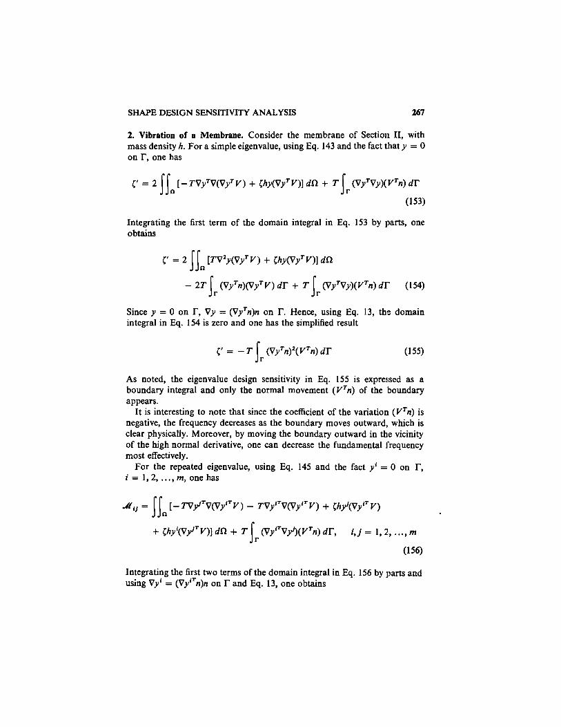
2. Vibration of a Membrane. Consider the membrane of Section 11, with mass density h. For a simple eigenvalue, using Eq. 143 and the fact that y = 0 on r, one has
Integrating the first term of the domain integral in Eq. 153 by parts, one obtains
- 2T 1 ( V y T n ) ( V y T ~ ) dT + T 1 (VyTVy)(VTn) d l . (154) I- I-
Since y = 0 on T , V y = (VyTn)n on l.. Hence, using Eq. 13, the domain integral in Eq. 154 is zero and one has the simplified result
(Vyrn)'(VTn) d l . (155)
As noted, the eigenvalue design sensitivity in Eq. 155 is expressed as a boundary integral and only the normal movement (VTn) of the 'boundary appears.
It is interesting to note that since the coefficient of the variation (VTn) is negative, the frequency decreases as the boundary moves outward, which is clear physically. Moreover, by moving the boundary outward in the vicinity of the high normal derivative, one can decrease the fundamental frequency most effectively.
For the repeated eigenvalue, using Eq. 145 and the fact y' = 0 on l., i = 1,2, . . . , m, one has
+ C ~ ~ ' ( V ~ ' ~ V ) ] dR + T ( V ~ ' ~ V ~ ' ) ( V ~ ~ ) dl., i, j = 1,2,, . . . , m 1 (156)
Integrating the first two terms of the domain integral in Eq. 156 by parts and using vyi = (vyi%)n on l. and Eq. 13, one obtains
Dow
nloa
ded
By:
[Uni
vers
ity o
f Iow
a Li
brar
ies]
At:
02:2
4 3
Febr
uary
200
8
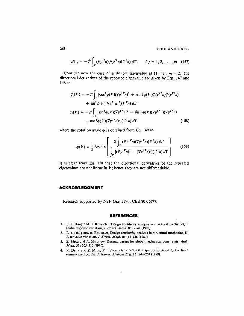
CHOI AND HAUG
Consider now the case of a double eigenvalue at R; i.e., m = 2. The directional derivatives of the repeated eigenvalue are given by Eqs. 147 and 148 as
[',(V) = - T [ C O ~ ~ ~ ( V ) ( V ~ ' ~ ~ ) ' + sin 24(V ) ( ~ y " n ) ( ~ y ~ ~ n ) J . (;(V) = - T 1 [ s i n ' ~ ( ~ ) ( V y ~ ~ n ] ~ - sin i ~ ( V ) ( ~ ~ ' ~ n ) ( ~ ~ ' ~ n )
r
where the rotation angle 4 is obtained fromEq. 149 as
It is clear from Eq. 158 that the directional derivatives of the repeated eigenvalues are not linear in V; hence they are not differentiable.
ACKNOWLEDGMENT
Research supported by NSF Grant No. CEE 80 05677.
REFERENCES
1. E. J . Haug and B. Rousselet, Design sensitivity analysis in structural mechanics, I. Static response variation, J. Strucf. Mech. 8 : 17-41 (1980).
2. E. J. Haug and B. Rousselet, Design sensitivity analysis in structural me~hanics, LI. Eigenvalue variation, J. Strucf. Me&. 8 : 161-186 (1980).
3. Z. Mroz and A. Mironow, Optimal design for global mechanical constraints, Arch. Mech. 32: 505-516 (1980).
4. K. Dems and Z. Mroz, Multiparameter structural shape optimization by the finite element method, Int. J. Numer. Mefhodr Eng. 13: 247-263 (1979).
Dow
nloa
ded
By:
[Uni
vers
ity o
f Iow
a Li
brar
ies]
At:
02:2
4 3
Febr
uary
200
8
SHAPE DESIGN SENSITIVITY ANALYSIS 269
5. K. Dems and Z. Mroz, Optimal shape design of multiwmposite stmcturs, J. Struct. Mech. 8 : 309-329 (1980).
6. J-P. Aubin, Applied Functional Analysis, Wiley-Interscience, New York, 1979. 7. R. A. Adams, Sobolev Spaces, Academic, New York, 1975. 8. I. S. Sokolnikoff, Mathematical Theory of Elasticity, McGraw-Hill, New York, 1956. 9. G. Fichera, Existence theorems in elasticity, Handbuch der Physik, VIn/2: 347-389
(1972). 10. W. H. Fleming, Functions of Several Variables, Addison-Wesley, Reading, Massa-
chusetts, 1965. 11. J-P. Zolesio, The material derivative (or speed) method for shape optimization, in
Optimization of Distributed Parameter Structures (E. J. Haug and J. Cea, eds.), Sijthoff & Noordhoff, Alphen aan den Rijn, Netherlands, 1981, pp. 1089-1151.
12. E. J. Haug, K. K. Choi, and V. Komkov, Structural Design Sensitivity Analysis, Academic, New York (in press).
13. B. Rousselet and E. J. Haug, Design sensitivity analysis of shape variations, in Optimi- zation of Distributed Parameter Structures ( E . J. Haug and J. Cea, eds.), Sijthoff & Noordhoff, Alphen aan den Rijn, Netherlands, 1981, pp. 1397-1442.
14. T. Kato, Perturbation Theory for Linear Operators, Springer, New York, 1976.
Received December I982