Embed Size (px)
Citation preview
R. L. Mokwa CHAPTER 2
6
CHAPTER 2
MECHANICS OF PILE CAP AND PILE GROUP
BEHAVIOR
2.1 INTRODUCTION
The response of a laterally loaded pile within a group of closely spaced piles is
often substantially different than a single isolated pile. This difference is attributed to the
following three items:
1. The rotational restraint at the pile cap connection. The
greater the rotational restraint, the smaller the deflection
caused by a given lateral load.
2. The additional lateral resistance provided by the pile
cap. As discussed in Chapter 1, verifying and
quantifying the cap resistance is the primary focus of
this research.
3. The interference that occurs between adjacent piles
through the supporting soil. Interference between zones
of influence causes a pile within a group to deflect more
than a single isolated pile, as a result of pile-soil-pile
interaction.
A comprehensive literature review was conducted as part of this research to
examine the current state of knowledge regarding pile cap resistance and pile group
behavior. Over 350 journal articles and other publications pertaining to lateral resistance,
testing, and analysis of pile caps, piles, and pile groups were collected and reviewed.
R. L. Mokwa CHAPTER 2
7
Pertinent details from these studies were evaluated and, whenever possible, assimilated
into tables and charts so that useful trends and similarities can readily be observed. Some
of the data, such as graphs that present p-multipliers as functions of pile spacing, are
utilized as design aids in subsequent chapters.
This chapter addresses three topics. The first is a review of the current state of
practice regarding the lateral resistance of pile caps. The second is a brief review of the
most recognized analytical techniques for analysis of single piles. This discussion of
single piles is necessary to set the stage for the third topic, which is a review of published
field and analytical research conducted to study the behavior of laterally loaded pile
groups.
2.2 PILE CAP RESISTANCE – STATE OF PRACTICE
A literature search was performed to establish the state of knowledge with regard
to pile cap resistance to lateral loads. The focus of the literature review was directed
towards experimental and analytical studies pertaining to the lateral resistance of pile
caps, and the interaction of the pile cap with the pile group.
There is a scarcity of published information available in the subject area of pile
cap lateral resistance. Of the publications reviewed, only four papers were found that
describe load tests performed to investigate the lateral resistance of pile caps. The results
from these four studies, summarized in Table 2.1 and Figure 2.1, show that the lateral
load resistance provided by pile caps can be very significant, and that in some cases the
cap resistance is as large as the resistance provided by the piles themselves.
Beatty (1970) tested two 6-pile groups of step-tapered piles and determined that
approximately 50 percent of the applied lateral load was resisted by passive pressure on
the pile cap.
R. L. Mokwa CHAPTER 2
8
Kim and Singh (1974) tested three 6-pile groups of 10BP42 piles and found that
removal of soil beneath the pile caps significantly increased the measured deflections,
rotations, and bending moments. This effect increased as the load increased.
Rollins et al. (1997) performed statnamic lateral testing on a group of 9 piles and
determined the lateral load resistance of the pile cap was greater than the lateral
resistance provided by the piles themselves.
Zafir and Vanderpool (1998) tested a group of four drilled shafts, two feet in
diameter, embedded in an 11-foot-diameter, 10-foot-thick cap, and determined that the
lateral load resistance of the cap was approximately equal to the lateral resistance
provided by the drilled shafts. Their measurements showed that the lateral resistance at
loads less than 450 tons was provided entirely by passive pressure on the cap.
No systematic method has been reported in the literature for unlinking the cap
resistance from the lateral resistance provided by the piles. For the most part, the studies
described above addressed only a portion of the cap resistance. For example, the
statnamic tests performed by Rollins et al. (1997) considered only the passive resistance
at the front of the cap, and only dynamic loads. Kim and Singh (1974) considered only
the soil in contact with the bottom of the pile cap. The pile caps in Kim and Singh’s
study were constructed on the ground surface, and thus the results do not include any
passive resistance at the front of the cap or frictional resistance of soil along the sides of
the cap. The tests by Beatty (1970) only involved the passive resistance at the front of
the cap. The tests by Zafir and Vanderpool (1998) were performed on an atypical pile
cap, which consisted of a large, deep circular embedded cap.
These studies indicate that the lateral resistance of pile caps can be quite
significant, especially when the pile cap is embedded beneath the ground surface. There
is clearly a need for a rational method to evaluate the magnitude of pile cap resistance,
and for including this resistance in the design of pile groups to resist lateral loads.
R. L. Mokwa CHAPTER 2
9
2.3 BEHAVIOR OF LATERALLY LOADED SINGLE PILES
Three criteria must be satisfied in the design of pile foundations subjected to
lateral forces and moments: 1) the soil should not be stressed beyond its ultimate
capacity, 2) deflections should be within acceptable limits, and 3) the structural integrity
of the foundation system must be assured.
The first criteria can be addressed during design using ultimate resistance theories
such as those by Broms (1964a, 1964b) or Brinch Hansen (1961). The second and third
criteria apply to deflections and stresses that occur at working loads. The behavior of
piles under working load conditions has been the focus of numerous studies over the past
40 to 50 years. A brief review of the most widely recognized analytical techniques is
provided in this section. Many of these techniques can be modified to predict the
behavior of closely spaced piles, or pile groups. Modifications for group response are
often in the form of empirically or theoretically derived factors that are applied, in
various ways, to account for group interaction effects.
Analytical methods for predicting lateral deflections, rotations and stresses in
single piles can be grouped under the following four headings:
• Winkler approach,
• p-y method,
• elasticity theory, and
• finite element methods.
These techniques provide a framework for the development of analytical
techniques that can be used to evaluate the response of piles in closely spaced groups,
which is the subject of Section 2.7.
R. L. Mokwa CHAPTER 2
10
2.3.1 Winkler Approach
The Winkler approach , also called the subgrade reaction theory, is the oldest
method for predicting pile deflections and bending moments. The approach uses
Winkler’s modulus of subgrade reaction concept to model the soil as a series of
unconnected linear springs with a stiffness, Es, expressed in units of force per length
squared (FL-2). Es is the modulus of soil reaction (or soil modulus) defined as:
yp
Es
−= Equation 2.1
where p is the lateral soil reaction per unit length of the pile, and y is the lateral deflection
of the pile (Matlock and Reese, 1960). The negative sign indicates the direction of soil
reaction is opposite to the direction of the pile deflection. Another term that is sometimes
used in place of Es is the coefficient (or modulus) of horizontal subgrade reaction, kh,
expressed in units of force per unit volume (Terzaghi 1955). The relationship between Es
and kh can be expressed as:
DkE hs = Equation 2.2
where D is the diameter or width of the pile. Es is a more fundamental soil property
because it is not dependent on the pile size. The behavior of a single pile can be analyzed
using the equation of an elastic beam supported on an elastic foundation (Hetenyi 1946),
which is represented by the 4th order differential beam bending equation:
02
2
4
4
=++ yEdx
ydQ
dx
ydIE spp Equation 2.3
where Ep is the modulus of elasticity of the pile, Ip is the moment of inertia of the pile
section, Q is the axial load on the pile, x is the vertical depth, and y is the lateral
deflection of the pile at point x along the length of the pile.
R. L. Mokwa CHAPTER 2
11
The governing equation for the deflection of a laterally loaded pile, obtained by
applying variational techniques (minimization of potential energy) to the beam bending
equation (Reddy 1993), and ignoring the axial component, is:
04
4
=+ yIE
E
dx
yd
pp
s Equation 2.4
Solutions to Equation 2.4 have been obtained by making simplifying assumptions
regarding the variation of Es (or kh) with depth. The most common assumption is that Es
is constant with depth for clays and Es varies linearly with depth for sands. Poulos and
Davis (1980) and Prakash and Sharma (1990) provide tables and charts that can be used
to determine pile deflections, slopes, and moments as a function of depth and non-
dimensional coefficients for a constant value of Es with depth.
The soil modulus for sand and normally consolidated clay is often assumed to
vary linearly with depth, as follows:
kxEs = Equation 2.5
where k (defined using the symbol nh by Terzaghi, 1955) is the constant of horizontal
subgrade reaction, in units force per volume. For this linear variation of Es with depth,
Matlock and Reese (1960) and Poulos and Davis (1980) present nondimensional
coefficients that can be used to calculate pile deflections, rotations, and bending moments
for various pile-head boundary conditions. Gill and Demars (1970) present other
formulations for the variation of Es with depth, such as step functions, hyperbolic
functions, and exponential functions.
The subgrade reaction method is widely employed in practice because it has a
long history of use, and because it is relatively straight forward to apply using available
chart and tabulated solutions, particularly for a constant or linear variation of Es with
depth. Despite its frequent use, the method is often criticized because of its theoretical
shortcomings and limitations. The primary shortcomings are:
R. L. Mokwa CHAPTER 2
12
1. the modulus of subgrade reaction is not a unique
property of the soil, but depends intrinsically on pile
characteristics and the magnitude of deflection,
2. the method is semi-empirical in nature,
3. axial load effects are ignored, and
4. the soil model used in the technique is discontinuous.
That is, the linearly elastic Winkler springs behave
independently and thus displacements at a point are not
influenced by displacements or stresses at other points
along the pile (Jamiolkowski and Garassino 1977).
Modifications to the original subgrade reaction approach have been proposed to
account for some of these shortcomings. One of these modifications attempts to convert
the Winkler model to a continuous model by coupling the springs using an inter-spring
shear layer component (Georgiadis and Butterfield 1982). This model also accounts for
the contribution of edge shear along the pile boundaries. The model has not gained
widespread acceptance because of difficulties associated with obtaining soil parameters
necessary to develop coefficients for use in the model (Horvath 1984).
McClelland and Focht (1956) augmented the subgrade reaction approach using
finite difference techniques to solve the beam bending equation with nonlinear load
versus deflection curves to model the soil. Their approach is known as the p-y method of
analysis. This method has gained popularity in recent years with the availability of
powerful personal computers and commercial software such as COM624 (1993) and
LPILE Plus3.0 (1997). A brief summary of the p-y method of analysis is presented in the
following section.
R. L. Mokwa CHAPTER 2
13
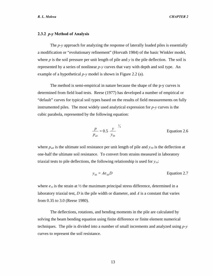
2.3.2 p-y Method of Analysis
The p-y approach for analyzing the response of laterally loaded piles is essentially
a modification or “evolutionary refinement” (Horvath 1984) of the basic Winkler model,
where p is the soil pressure per unit length of pile and y is the pile deflection. The soil is
represented by a series of nonlinear p-y curves that vary with depth and soil type. An
example of a hypothetical p-y model is shown in Figure 2.2 (a).
The method is semi-empirical in nature because the shape of the p-y curves is
determined from field load tests. Reese (1977) has developed a number of empirical or
“default” curves for typical soil types based on the results of field measurements on fully
instrumented piles. The most widely used analytical expression for p-y curves is the
cubic parabola, represented by the following equation:
31
50
5.0
=
yy
pp
ult
Equation 2.6
where pult is the ultimate soil resistance per unit length of pile and y50 is the deflection at
one-half the ultimate soil resistance. To convert from strains measured in laboratory
triaxial tests to pile deflections, the following relationship is used for y50:
DAy 5050 ε= Equation 2.7
where ε50 is the strain at ½ the maximum principal stress difference, determined in a
laboratory triaxial test, D is the pile width or diameter, and A is a constant that varies
from 0.35 to 3.0 (Reese 1980).
The deflections, rotations, and bending moments in the pile are calculated by
solving the beam bending equation using finite difference or finite element numerical
techniques. The pile is divided into a number of small increments and analyzed using p-y
curves to represent the soil resistance.
R. L. Mokwa CHAPTER 2
14
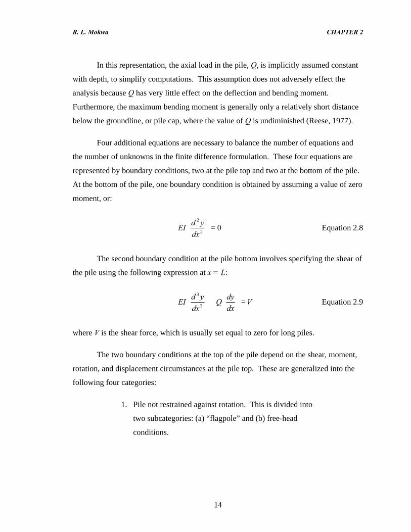
In this representation, the axial load in the pile, Q, is implicitly assumed constant
with depth, to simplify computations. This assumption does not adversely effect the
analysis because Q has very little effect on the deflection and bending moment.
Furthermore, the maximum bending moment is generally only a relatively short distance
below the groundline, or pile cap, where the value of Q is undiminished (Reese, 1977).
Four additional equations are necessary to balance the number of equations and
the number of unknowns in the finite difference formulation. These four equations are
represented by boundary conditions, two at the pile top and two at the bottom of the pile.
At the bottom of the pile, one boundary condition is obtained by assuming a value of zero
moment, or:
02
2
=
dx
ydEI Equation 2.8
The second boundary condition at the pile bottom involves specifying the shear of
the pile using the following expression at x = L:
Vdxdy
Qdx
ydEI =
+
3
3
Equation 2.9
where V is the shear force, which is usually set equal to zero for long piles.
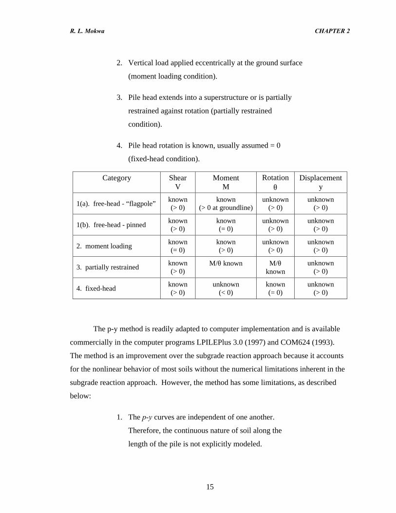
The two boundary conditions at the top of the pile depend on the shear, moment,
rotation, and displacement circumstances at the pile top. These are generalized into the
following four categories:
1. Pile not restrained against rotation. This is divided into
two subcategories: (a) “flagpole” and (b) free-head
conditions.
R. L. Mokwa CHAPTER 2
15
2. Vertical load applied eccentrically at the ground surface
(moment loading condition).
3. Pile head extends into a superstructure or is partially
restrained against rotation (partially restrained
condition).
4. Pile head rotation is known, usually assumed = 0
(fixed-head condition).
Category ShearV
MomentM
Rotationθ
Displacementy
1(a). free-head - “flagpole”known(> 0)
known(> 0 at groundline)
unknown(> 0)
unknown(> 0)
1(b). free-head - pinnedknown(> 0)
known(= 0)
unknown(> 0)
unknown(> 0)
2. moment loadingknown(= 0)
known(> 0)
unknown(> 0)
unknown(> 0)
3. partially restrainedknown(> 0)
M/θ known M/θknown
unknown(> 0)
4. fixed-headknown(> 0)
unknown(< 0)
known(= 0)
unknown(> 0)
The p-y method is readily adapted to computer implementation and is available
commercially in the computer programs LPILEPlus 3.0 (1997) and COM624 (1993).
The method is an improvement over the subgrade reaction approach because it accounts
for the nonlinear behavior of most soils without the numerical limitations inherent in the
subgrade reaction approach. However, the method has some limitations, as described
below:
1. The p-y curves are independent of one another.
Therefore, the continuous nature of soil along the
length of the pile is not explicitly modeled.
R. L. Mokwa CHAPTER 2
16
2. Suitable p-y curves are required. Obtaining the
appropriate p-y curve is analogous to obtaining the
appropriate value of Es; one must either perform full-
scale instrumented lateral load tests or adapt the
existing available standard curves (default curves) for
use in untested conditions. These default curves are
limited to the soil types in which they were developed;
they are not universal.
3. A computer is required to perform the analysis.
Other representations of p-y curves have been proposed such as the hyperbolic
shape by (Kondner 1963). Evans (1982) and Mokwa et al. (1997) present a means of
adjusting the shape of the p-y curve to model the behavior of soils that have both
cohesion and friction using Brinch Hansen’s (1961) φ-c ultimate theory. In situ tests such
as the dilatometer (Gabr 1994), cone penetrometer (Robertson et al. 1985), and
pressuremeter (Ruesta and Townsend 1997) have also been used to develop p-y curves.
2.3.3 Elasticity Theory
Poulos (1971a, 1971b) presented the first systematic approach for analyzing the
behavior of laterally loaded piles and pile groups using the theory of elasticity. Because
the soil is represented as an elastic continuum, the approach is applicable for analyzing
battered piles, pile groups of any shape and dimension, layered systems, and systems in
which the soil modulus varies with depth. The method can be adapted to account for the
nonlinear behavior of soil and provides a means of determining both immediate and final
total movements of the pile (Poulos 1980).
Poulos’s (1971a, 1971b) method assumes the soil is an ideal, elastic,
homogeneous, isotropic semi-infinite mass, having elastic parameters Es and vs. The pile
is idealized as a thin beam, with horizontal pile deflections evaluated from integration of
R. L. Mokwa CHAPTER 2
17
the classic Mindlin equation for horizontal subsurface loading. The Mindlin equation is
used to solve for horizontal displacements caused by a horizontal point load within the
interior of a semi-infinite elastic-isotropic homogeneous mass. Solutions are obtained by
integrating the equation over a rectangular area within the mass. The principle of
superposition is used to obtain displacement of any points within the rectangular area.
Details of the Mindlin equation can be found in Appendix B of Pile Foundation Analysis
and Design by Poulos and Davis (1980).
The pile is assumed to be a vertical strip of length L, width D (or diameter, D, for
a circular pile), and flexural stiffness EpIp. It is divided into n+1 elements and each
element is acted upon by a uniform horizontal stress p. The horizontal displacements of
the pile are equal to the horizontal displacements of the soil. The soil displacements are
expressed as:
}]{[}{ pIEd
y s
s
s = Equation 2.10
where {ys} is the column vector of soil displacements, {p} is the column vector of
horizontal loading between soil and pile, and [Is] is the n+1 by n+1 matrix of soil-
displacement influence factors determined by integrating Mindlin’s equation, using
boundary element analyses (Poulos 1971a). The finite difference form of the beam
bending equation is used to determine the pile displacements. The form of the equation
varies depending on the pile-head boundary conditions. Poulos and Davis (1980) present
expressions for free-head and fixed-head piles for a number of different soil and loading
conditions. One of the biggest limitations of the method (in addition to computational
complexities) is the difficulty in determining an appropriate soil modulus, Es.
2.3.4 Finite Element Method
The finite element method is a numerical approach based on elastic continuum
theory that can be used to model pile-soil-pile interaction by considering the soil as a
three-dimensional, quasi-elastic continuum. Finite element techniques have been used to
R. L. Mokwa CHAPTER 2
18
analyze complicated loading conditions on important projects and for research purposes.
Salient features of this powerful method include the ability to apply any combination of
axial, torsion, and lateral loads; the capability of considering the nonlinear behavior of
structure and soil; and the potential to model pile-soil-pile-structure interactions. Time-
dependent results can be obtained and more intricate conditions such as battered piles,
slopes, excavations, tie-backs, and construction sequencing can be modeled. The method
can be used with a variety of soil stress-strain relationships, and is suitable for analyzing
pile group behavior, as described in Section 2.7.5. Performing three-dimensional finite
element analyses requires considerable engineering time for generating input and
interpreting results. For this reason, the finite element method has predominately been
used for research on pile group behavior, rarely for design.
2.4 PILE GROUP BEHAVIOR – EXPERIMENTAL RESEARCH
2.4.1 Background
The literature review also encompassed the current state of practice in the area of
pile group behavior and pile group efficiencies. This section describes relevant aspects of
experimental studies reported in the literature. Analytical studies of pile group behavior
are described in Section 2.7.
Table A.1 (located in Appendix A) contains a summary of 37 experimental
studies in which the effects of pile group behavior were observed and measured. The
table includes many relevant load tests that have been performed on pile groups during
the past 60 years. The references are organized chronologically. Multiple references
indicate that a particular test was addressed in more than one published paper.
The conventions and terms used to describe pile groups in this dissertation are
shown in Figure 2.3. Most pile groups used in practice fall into one of the following
three categories, based on the geometric arrangement of the piles:
R. L. Mokwa CHAPTER 2
19
1. Figure 2.3 (a) – in-line arrangement. The piles are
aligned in the direction of load.
2. Figure 2.3 (b) – side-by-side arrangement. The piles
are aligned normal to the direction of load.
3. Figure 2.3 (c)– box arrangement. Consists of multiple
in-line or side-by-side arrangements.
Pile rows are labeled as shown in Figure 2.3(c). The leading row is the first row
on the right, where the lateral load acts from left to right. The rows following the leading
row are labeled as 1st trailing row, 2nd trailing row, and so on. The spacing between two
adjacent piles in a group is commonly described by the center to center spacing,
measured either parallel or perpendicular to the direction of applied load. Pile spacings
are often normalized by the pile diameter, D. Thus, a spacing identified as 3D indicates
the center to center spacing in a group is three times the pile diameter. This convention is
used throughout this document.
The experimental studies described in Table A1 are categorized under three
headings:
1. full-scale field tests (15 studies)
2. 1g model tests (16 studies)
3. geotechnical centrifuge tests (6 studies)
Pertinent details and relevant test results are discussed in the following sections.
2.4.2 Full-Scale Field Tests
Full-scale tests identified during the literature review include a wide variety of
pile types, installation methods, soil conditions, and pile-head boundary conditions, as
shown in Table 2.2.
R. L. Mokwa CHAPTER 2
20
The earliest reported studies (those by Feagin and Gleser) describe the results of
full-scale field tests conducted in conjunction with the design and construction of large
pile-supported locks and dams along the Mississippi River. O’Halloran (1953) reported
tests that were conducted in 1928 for a large paper mill located in Quebec City, Canada,
along the banks of the St. Charles River. Load tests performed in conjunction with the
Arkansas River Navigation Project provided significant amounts of noteworthy design
and research data, which contributed to advancements in the state of practice in the early
1970’s. Alizadeh and Davisson (1970) reported the results of numerous full-scale lateral
load tests conducted for navigation locks and dams that were associated with this massive
project, located in the Arkansas River Valley.
Ingenious methods were devised in these tests for applying loads and monitoring
deflections of piles and pile groups. The load tests were usually conducted during design
and, very often, additional tests were conducted during construction to verify design
assumptions. In many instances, the tests were performed on production piles, which
were eventually integrated into the final foundation system.
The most notable difference between the tests conducted prior to the 1960’s and
those conducted more recently is the sophistication of the monitoring instruments.
Applied loads and pile-head deflection were usually the only variables measured in the
earlier tests. Loads were typically measured manually by recording the pressure gauge
reading of the hydraulic jack.
A variety of methods were employed to measure deflections. In most cases, more
than one system was used to provide redundancy. For example, Feagin (1953) used two
completely independent systems. One system used transit and level survey instruments,
and the other system consisted of micrometers, which were embedded in concrete and
connected to piano wires under 50 pound of tension. Electronic contact signals were
used to make the measurements with a galvanometer connected in series with a battery.
O’Halloran (1953) manually measured horizontal deflections using piano wire as a point
of reference. The piano wires, which were mounted outside the zone of influence of the
R. L. Mokwa CHAPTER 2
21
test, were stretched across the centerline of each pile, at right angles to the direction of
applied load. Deflection measurements were made after each load application by
measuring the horizontal relative displacement between the pile center and the piano
wire.
Over the last 30 to 40 years, the level of sophistication and overall capabilities of
field monitoring systems have increased with the advent of personal computers and
portable multi-channel data acquisition systems. Hydraulic rams or jacks are still
commonly used for applying lateral loads for static testing. However, more advanced
systems are now used for cyclic and dynamic testing. Computer-driven servo-controllers
are often used for applying large numbers of cyclic loads. For example, Brown and
Reese (1985) applied 100 to 200 cycles of push-pull loading at 0.067 Hz using an MTS
servo valve operated by an electro-hydraulic servo controller.
A variety of methods have been used to apply dynamic loads. Blaney and O’Neill
(1989) used a linear inertial mass vibrator to apply dynamic loads to a 9-pile group at
frequencies as high as 50 Hz. Rollins et al. (1997) used a statnamic loading device to
apply large loads of short duration (100 to 250 msec) to their test pile group. The
statnamic device produces force by igniting solid fuel propellant inside a cylinder
(piston), which causes a rapid expansion of high-pressure gas that propels the piston and
forces the silencer and reaction mass away.
Powerful electronic systems are now available to facilitate data collection. These
systems usually have multiple channels for reading responses from a variety of
instruments at the same time. It is now possible to collect vast amounts of information
during a test at virtually any frequency and at resolutions considerably smaller than is
possible using optical or mechanical devices.
Pile deflections and rotations are often measured using displacement transducers,
linear potentiometers, and linear variable differential transformers (LVDT’s). In addition
to measuring deflections, piles are often instrumented with strain gauges and slope
R. L. Mokwa CHAPTER 2
22
inclinometers. Information obtained from these devices can be used to calculate stresses,
bending moments, and deflections along the length of a pile.
Whenever possible, strain gauges are installed after the piles are driven to
minimize damage. A technique commonly used with closed-end pipe piles is to attach
strain gauges to a smaller diameter steel pipe or sister bar, which is then inserted into the
previously driven pile and grouted in place. This method was used in the tests performed
on pipe piles by Brown (1985), Ruesta and Townsend (1997), and Rollins et al. (1998).
In some cases, strain gauges are attached prior to installing piles. For instance,
gauges are often attached to steel H-piles prior to driving; or gauges may be attached to
the reinforcing steel cage prior to pouring concrete for bored piles (drilled shafts).
Meimon et al. (1986) mounted strain gauges on the inside face of the pile flange and
mounted a slope inclinometer tube on the web face. They protected the instruments by
welding steel plates across the ends of the flanges creating a boxed-in cross-section, and
drove the piles close-ended.
Applied loads are usually measured using load cells. Ruesta and Townsend
(1997) used ten load cells for tests on a 9-pile group. One load cell was used to measure
the total applied load, and additional load cells were attached to the strut connections at
each pile. Additional instruments such as accelerometers, geophones, and earth pressure
cells are sometimes used for specialized applications.
2.4.3 1g Model Tests
The majority of experiments performed on pile groups fall under the category of
1g model tests. Model tests are relatively inexpensive and can be conducted under
controlled laboratory conditions. This provides an efficient means of investigation. For
instance, Cox et al. (1984) reported on a study in which tests on 58 single piles and 41
pile groups were performed. They varied the geometric arrangement of piles within
groups, the number of piles per group, and the spacing between piles. Liu (1991)
performed 28 sets of tests on pile groups in which the pile spacing, group configuration,
R. L. Mokwa CHAPTER 2
23
and pile lengths were varied. Franke (1988) performed a number of parametric studies
by varying the arrangement, size, and spacing of piles within groups; the length and
stiffness of the piles; the pile head boundary conditions; and the relative density of the
backfill soil.
Aluminum is the most frequently used material for fabricating model piles. Small
diameter aluminum pipes, bars, or tubes were used in 8 of the 16 model tests reported in
Table A.1. Other materials such as mild steel and chloridized-vinyl (Shibata et al. 1989)
have also been used. Tschebotarioff (1953) and Wen (1955) used small wood dowels to
represent timber piles in their model tests
Sand was by far the most commonly used soil (12 out of 16 tests); however, silt
and clay soils were used as well. A variety of techniques were used to place soil and
install piles. In some studies, soil was placed first and the piles were subsequently
driven, pushed or bored into place. In other cases, the piles were held in place as soil was
placed around them. Techniques for installing soil included tamping, pluviation, raining,
dropping, flooding, and “boiling”. Shibata et al. (1989) applied the term boiling to the
technique of pumping water with a strong upward gradient through the bottom of a sand-
filled tank.
The primary shortcomings of 1g model testing are related to scaling and edge
effects. Scaling effects limit the applicability of model tests in simulating the
performance of prototypes. Models are useful in performing parametric studies to
examine relative effects, but it is appropriate to exercise caution in extrapolating results
obtained from model tests to full-scale dimensions. Items such as at-rest stress levels,
soil pressure distributions, and soil particle movements are all factors influenced by
scaling (Zhang and Hu 1991).
Edge effects become significant if the size of the test tank is too small relative to
the size of the model pile. Prakash (1962) reported the results of tests in a large test tank
in which the zone of influence (or zone of interference) extended a distance of 8 to 12
R. L. Mokwa CHAPTER 2
24
times the pile width in the direction of loading and 3 to 4 times the pile width normal to
the direction of loading. Experimental apparatus that do not meet these guidelines would
involve edge effects, which are not easily quantified.
As discussed in the following paragraphs, centrifuge tests have become
increasingly popular in the last decade as a means of overcoming scaling effects inherent
in 1g model testing.
2.4.4 Centrifuge Tests
Similar to 1g model testing, a geotechnical centrifuge provides a relatively rapid
method for performing parametric studies. The advantage of centrifuge modeling lies in
the ability of the centrifuge to reproduce prototype stress-strain conditions in a reduced
scale model (Mcvay et al. 1995).
For additional information pertaining to centrifuge mechanics, the reader is
referred to the 20th Rankine Lecture by Schofield (1980), which provides a detailed
discussion of centrifuge testing principles. Schofield explains the mechanics behind
centrifuge modeling in terms of Newtonian physics and the theory of relativity. In
essence, the gravitational force of a prototype body is indistinguishable from, and
identical to, an inertial force created in the centrifuge. Thus, if the product of depth times
acceleration is the same in model and prototype, the stresses at every point within the
model will theoretically be the same as the stresses at every corresponding point in the
prototype (Schofield 1980).
Four studies that investigated the lateral resistance of pile groups using
geotechnical centrifuges were found during the literature study, and these are summarized
in Table A.1. Some details about the facilities are provided in Table 2.3. Significant
aspects of the studies are discussed in the following paragraphs.
The first centrifuge tests on model pile groups were performed by Barton (1984)
on groups consisting of 2, 3, and 6 piles at various spacings and orientations with respect
R. L. Mokwa CHAPTER 2
25
to the direction of load. Zhang and Hu (1991) examined the effect of residual stresses on
the behavior of laterally loaded piles and pile groups. Adachi et al. (1994b) examined
pile-soil-pile interaction effects by testing two piles at various spacings and orientations.
In these three studies, the soil was placed and the piles were installed prior to starting the
centrifuge (i.e., pile installation occurred at 1g).
McVay et al. (1994) was the first to install pile groups in flight, laterally load
them, and measure their response without stopping the centrifuge. The results from
McVay’s study indicates that piles have greater resistance to lateral and axial loads when
driven at prototype stress levels (centrifuge in motion during pile installation), as opposed
to 1g installation. The difference in behavior is attributed to the significantly greater
dilation of the test sand at 1g and resulting decrease in density and strength (McVay et al.
1995).
McVay et al. (1994, 1995, and 1998) measured group efficiencies and back-
calculated p-multipliers for pile groups ranging in size from 3 by 3 to 3 by 7 (3 rows
oriented parallel to the direction of loading and 7 rows oriented normal to the direction of
load). Spacings of 3 and 5 times the pile diameter were tested using both loose- and
medium-dense sand backfill.
Centrifuge testing appears to provide a relatively efficient means of systematically
investigating several variables at prototype stress conditions. Factors that impact
centrifuge test results include boundary conditions or edge effects between the model
foundation and the centrifuge bucket (model container), and soil behavior incongruities
caused by installing piles at 1g, rather than in flight. Additional inconsistencies between
model and prototype behavior may arise when testing clayey soils. Schofield (1980)
describes these limitations and attributes them to changes in water contents, pore
pressures, and equivalent liquidities, which are difficult to model in the centrifuge.
R. L. Mokwa CHAPTER 2
26
2.5 PILE GROUP EFFICIENCY
2.5.1 Background
Piles are usually constructed in groups and tied together by a concrete cap at the
ground surface. Piles in closely spaced groups behave differently than single isolated
piles because of pile-soil-pile interactions that take place in the group. It is generally
recognized that deflections of a pile in a closely spaced group are greater than the
deflections of an individual pile at the same load because of these interaction effects. The
maximum bending moment in a group will also be larger than that for a single pile,
because the soil behaves as if it has less resistance, allowing the group to deflect more for
the same load per pile.
The most widely recognized standard for quantifying group interaction effects is
the group efficiency factor, Ge, which is defined in Equation 2.11 as the average lateral
capacity per pile in a group divided by the lateral capacity of a single pile (Prakash 1990).
( )( )
su
gu
e Qn
QG = Equation 2.11
Where (Qu)g is the ultimate lateral load capacity of the group, n is the number of
piles in the group, and (Qu)s is the ultimate lateral load capacity of a single pile. A
somewhat different definition for the group efficiency factor, one that is based on p-
multipliers, is described in Section 2.6.
The analysis of pile group behavior can be divided into widely-spaced closely-
spaced piles. Model tests and a limited number of full-scale tests indicate that piles are
not influenced by group effects if they are spaced far apart.
Piles installed in groups at close spacings will deflect more than a single pile
subjected to the same lateral load per pile because of group effects (Bogard and Matlock,
1983). There is general agreement in the literature that group effects are small when
R. L. Mokwa CHAPTER 2
27
center-to-center pile spacings exceed 6 pile diameters (6D) in a direction parallel to the
load and when they exceed 3D measured in a direction perpendicular to the load. This
approximation has been validated through experimental tests by Prakash (1967), Franke
(1988), Lieng (1989), and Rao et al. (1996).
Group efficiency factors can be evaluated experimentally by performing load tests
on pile groups and on comparable single piles. The next section summarizes over 60
years of experimental research in the area of pile group efficiencies.
2.5.2 Group Efficiency Factors
Fourteen of the studies included in Table A.1 involve experimental evaluations of
the group efficiency factor, Ge, or provide enough information to calculate Ge using
Equation 2.11. The references for these 14 studies are tabulated chronologically in Table
2.4. Pertinent data from these papers are presented in Table 2.4 for three geometric
arrangements, defined in Figure 2.3 as: box, in-line, and side-by-side. Some of the
references, such as Cox et al. (1984) and Shibata et al. (1989), include multiple tests
conducted using different geometric arrangements and pile spacings. For clarity, these
tests were arranged into separate rows of the table. Of the 85 separate tests described in
Table 2.4, only five percent (4 tests) were full-scale. The remaining tests were performed
on reduced scale models, either 1g model or centrifuge. The large percentage of model
tests is due to the relative ease and lower cost of these tests, as opposed to full-scale field
tests.
The studies summarized in Table 2.4 were examined in detail to determine the
factors that most significantly effect overall group efficiency. Because most of these
factors are interrelated, those with greatest significance are identified first. In order of
importance, these factors are:
• pile spacing
• group arrangement
R. L. Mokwa CHAPTER 2
28
• group size
• pile-head fixity
• soil type and density
• pile displacement
Pile Spacing
Center to center pile spacing is the dominant factor affecting pile group
efficiency. Cox et al. (1984) measured group efficiencies ranging from 0.59 at 1.5D
spacing to 0.95 at 3D spacing for a 3-pile in-line arrangement in very soft clay. For the
same arrangement of piles in medium dense sand, Sarsby (1985) reported nearly the same
values of group efficiencies ranging from 0.66 at 2D spacing to 0.80 at 8D spacing.
The results for all of the tests summarized in Table 2.4, are plotted in Figure 2.4
as a function of center to center pile spacing. The most significant trend in this figure is
the increase of Ge with pile spacing. However, there is a large amount of scatter in the
data indicating that other factors also influence the value of Ge. To estimate accurate
values of group efficiency, it is necessary to consider factors in addition to pile spacing.
Group Arrangement and Group Size
After pile spacing, the next most significant factor appears to be the geometric
arrangement of piles within the group. Observable trends are evident in Figure 2.4,
where the group arrangements (square, in-line, and side-by-side) are delineated using
different symbols. Piles in square arrangements are represented by solid squares, in-line
arrangements are identified by solid circles, and side-by-side arrangements are identified
by open circles. The three outlying data points (shown as solid circles) at 8D spacing
represent results from Sarsby’s (1985) 1g model tests. These tests were performed on
small (less than ¼-inch-diameter) steel bars. The bars were repeatedly pushed laterally to
deflections greater than 20 times the pile diameter, and Ge values were determined by
extrapolating the resistance curves back to zero deflection. Because the test procedure is
R. L. Mokwa CHAPTER 2
29
questionable, and the results are not consistent with those from other more reasonable test
procedures, no weight is placed on these tests in the development of recommendations for
design.
For clarity, the test results are plotted and described separately based on the
arrangement of piles within a group, as follows:
• box arrangement - Figures 2.5 and 2.6
• in-line arrangement – Figures 2.7 and 2.8
• side-by-side arrangement - Figure 2.9
Design curves were visually fitted through the data points for the three types of
pile arrangements, using engineering judgement, as described below.
Box arrangement. Test results from Table 2.4 for multiple rows of piles oriented
in box arrangements are plotted in Figure 2.5, along with the proposed design curve. The
design curve is linear between Ge = 1.0 at a spacing of 6D, and Ge = 0.25 at a spacing of
1D.
There is no clear effect of group size, as can be seen in Figure 2.6. This may be a
result of scatter in the data. One could logically infer that shadowing effects would
increase with group size. If this were the case, group efficiency would be expected to
decrease as group size increased. As additional data becomes available, it may be
possible to quantify the effect of group size.
In-line arrangement. Test results from Table 2.4 for single rows of piles
oriented in the direction of load (in-line arrangement) are plotted in Figure 2.7, along
with proposed design lines. Based on this plot, it can be noted that group efficiency is
influenced by the number of piles in the line. This can be seen more clearly in Figure
2.8, where the data points are plotted using symbols that indicate the number of piles per
line, either 2, 3, or 4. The following conclusions can be drawn from this plot:
R. L. Mokwa CHAPTER 2
30
1. At the same pile spacing, a single row of in-line piles
will have a greater group efficiency than piles in a box
arrangement.
2. At a given spacing, the group efficiency decreases as
the number of piles in a line increase.
As additional data become available, it may be possible to refine the design lines
shown in Figures 2.7 and 2.8.
Side-by-side arrangement. Test results from Table 2.4 for single rows of piles
oriented normal to the direction of load (side-by-side arrangement) are plotted in Figure
2.9, along with the proposed design line. From this plot, it is concluded that:
1. Piles oriented in side-by-side arrangements are effected
by pile spacing to a lesser degree than in-line or box
arrangements of piles.
2. For practical purposes, side-by-side piles spaced at 3D
or greater experience no group effects. In other words,
side-by-side piles spaced at 3D or greater will behave
the same as single isolated piles.
Pile Head Fixity
Approximately 80 % of the tests described in Table 2.4 were reportedly
performed on free-headed piles, with either pinned or “flag pole” boundary conditions.
The remaining 20 % of the tests were performed on piles with fixed-head boundary
conditions. It is postulated, that the boundary conditions for some of the tests reported in
Table 2.4 were partially restrained, rather than fixed or free headed. Significant
conclusions regarding the impact of pile head restraint on group efficiency are not
possible because of inconsistencies regarding the classification of boundary conditions
and the small number of fixed-headed tests. The unequal distribution of boundary
R. L. Mokwa CHAPTER 2
31
conditions among the tests becomes even more significant when the data is divided into
subgroups based on geometric characteristics (i.e., box, in-line, and side-by-side).
Determining the actual degree of fixity under which test piles are loaded is
probably a more significant issue than ascertaining the effect that pile-head fixity has on
the value of Ge. To determine Ge by direct comparison, the boundary condition for the
piles in the group should be the same as the single pile boundary condition. If this is not
the case, than Ge may be evaluated inaccurately. For free-headed piles, this
determination is not difficult. However, it is very difficult to achieve completely fixed-
head conditions for single piles and pile groups. As discussed subsequently in the section
on p-multipliers, there are other approaches available for determining Ge that can be used
if the boundary conditions of the group do not match those of the single pile. However,
for these methods to yield accurate results, the boundary conditions must be known.
Soil Type and Density
Sixty-six percent of the tests described in Table 2.4 were performed in sand, 27 %
in clay, and 7 % in silt. The results are plotted in Figure 2.10 as a function of soil type,
for piles in box arrangements. There does not appear to be any significant trends in this
data, except possibly for the tests performed in silty soil. These tests were performed by
Prakash and Saran (1967) and appear to yield slightly lower Ge values then tests
performed in clay or sand, at comparable spacings. However, because these were the
only tests performed using silty soil and the points are not far below the design line, it
seems reasonable to use the same design lines for piles in silt.
The following three studies provide useful information pertaining to the
sensitivity of Ge to soil type or soil density.
1.) McVay et al. (1995) performed centrifuge tests on pile
groups embedded in loose and medium dense sand at
3D and 5D spacings. From these studies, they
R. L. Mokwa CHAPTER 2
32
concluded that group efficiency is independent of soil
density.
2.) Two separate studies were performed on the same 3 by
3 pile group at a site in Texas. The first series of tests
were performed with the piles embedded in native
clayey soils, and a Ge of 0.75 was determined (Brown
and Reese 1985). The second series of tests were
performed after the native soils were replaced with
compacted sand. The Ge determined in this case was
0.77, almost exactly the same as for piles in clay. Thus,
changing the soil type from a stiff clay to a medium
dense sand had essentially no effect on the measured
Ge.
3.) Brown and Shie (1991) investigated group efficiencies
using detailed three-dimensional finite element analyses
with two different soil models, Von Mises for saturated
clay and extended Drucker-Prager for sand. They
concluded that the variation in group efficiencies
between the two models was too small to warrant
consideration in design.
In general, it appears that soil type and soil density do not significantly affect pile
group efficiencies.
Pile Displacement
Group efficiency as defined in Equation 2.11 is independent of pile displacement.
It remains to be determined, however, whether Ge varies with pile displacement, all other
things being equal. To gain insight into this question, results from six of the studies
described in Table 2.4 were used to calculate values of group efficiency for a range of
R. L. Mokwa CHAPTER 2
33
pile displacements. The results of these calculations are plotted in Figure 2.11. Based on
these plots, it appears that Ge first decreases as displacement increases, and then becomes
constant at deflections in excess of 0.05D (5 % of the pile diameter). The small
variations in Ge at deflections greater than 0.05D fall within the typical range of
experimental data scatter, and are insignificant with respect to practical design
considerations.
The proposed design curves presented in Figures 2.5 through 2.10 were computed
using data for deflections greater than 0.05D. Based on the review of available literature,
this appears reasonable, and will yield conservative results for deflections less than
0.05D.
The writer believes that the design curves presented in this section, which are
based on the compilation of experimental evidence in Table 2.4, represent the best and
most complete values of Ge that can be currently established. They are recommended as
state-of-the-art values for use in analysis and design of laterally loaded pile groups.
2.6 P-MULTIPLIERS
2.6.1 Background
Measurements of displacements and stresses in full-scale and model pile groups
indicate that piles in a group carry unequal lateral loads, depending on their location
within the group and the spacing between piles. This unequal distribution of load among
piles is caused by “shadowing”, which is a term used to describe the overlap of shear
zones and consequent reduction of soil resistance. A popular method to account for
shadowing is to incorporate p-multipliers into the p-y method of analysis. The p-
multiplier values depend on pile position within the group and pile spacing. This section
summarizes the current state of knowledge pertaining to p-multipliers, and presents
recommendations based on a compilation of available research data.
R. L. Mokwa CHAPTER 2
34
The concept of p-multipliers (also called fm) were described by Brown et al.
(1988) as a way of accounting for pile group effects by making adjustments to p-y curves.
The multipliers are empirical reduction factors that are experimentally derived from load
tests on pile groups. Because they are determined experimentally, the multipliers include
both elasticity and shadowing effects. This eliminates the need for a separate y-
multiplier, which is found in many elasticity-based methods. The procedure follows the
same approach used in the p-y method of analysis, except that a multiplier, with a value
less than one, is applied to the p-values of the single pile p-y curve. This reduces the
ultimate soil resistance and softens the shape of the p-y curve, as shown in Figure 2.2 (b).
Table 2.5 summarizes the results from 11 experimental studies, which present p-
multipliers for pile groups of different sizes and spacings. In these studies, which include
29 separate tests, p-multipliers were determined through a series of back-calculations
using results from instrumented pile-group and single pile load tests. The general
procedure for calculating multipliers from load tests results is summarized below.
Step 1 – Assemble load test data. Data is required from lateral load tests
performed on groups of closely spaced piles and a comparable single pile. At a
minimum, the instrumentation program should provide enough data to develop load
versus deflection curves for each pile in the group and the single pile. Ideally, the piles
will be fully instrumented so that deflections are measured at the top of each pile and
strains caused by bending and deformation are measured throughout the length of the
piles.
Step 2 – Develop and adjust single pile p-y curves. The goal of this step is to
develop a set of p-y curves that accurately model the soil conditions at the test site based
on the measured load response of the single pile. Trial p-y curves, determined by any
suitable method, are adjusted until a good match is obtained between the calculated and
the measured response of the single pile.
R. L. Mokwa CHAPTER 2
35
Step 3 – Determine fm values. The multipliers are determined in this step
through a trial and error process using the p-y curves developed for the single pile and the
measured load versus deflection responses for piles in the group. Trial values of fm are
adjusted until a good match is obtained between the measured and calculated load versus
deflection response curves for each pile.
2.6.2 Experimental Studies
Brown and Reese (1985), Morrison and Reese (1986), and McVay et al. (1995)
did not detect any significant variation in the response of individual piles within a given
row; therefore, they used average response curves for each row of piles rather than
attempting to match the response curves for every pile in the group. A similar approach
was used by Ruesta and Townsend (1997) and Rollins et al. (1998). In all of these cases,
loads were essentially the same for piles in a given row. The current state of practice is
thus to use individual row multipliers, rather than separate multipliers for each pile. This
approach was followed in all of the studies reported in Table 2.5.
The similarity in behavior between piles in a row is attributed to the pile spacing,
which ranged from 3D to 5D in the studies described herein. As discussed in the group
efficiency section (see Figure 2.9), side-by-side piles at spacings greater than or equal to
3D are not affected by adjacent piles in the same row. However, at spacings less than
3D, the outer corner piles will take a greater share of load than the interior piles, as
demonstrated in Franke’s (1988) model tests, and as supported by elasticity-based
methods (Poulos 1971b). This implies that corner piles will experience greater bending
moments and stresses than interior piles at spacings less than 3D. Ignoring this behavior
is unconservative, and could results in overstressed corner piles (in the leading row) for
piles spaced at less than 3D.
Franke (1988) performed model tests on 3 side-by-side piles and measured the
load that was taken up by each pile. At 3D spacing, the load distribution between the
corner piles and center pile was the same. At 2D spacing the corner piles resisted 20 %
R. L. Mokwa CHAPTER 2
36
more load than the center pile, and at 1D spacing the corner piles resisted 60 % more
load.
The generally accepted approach is to assumed that p-multipliers are constant
with depth. That is, a constant p-multiplier is applied to the set of p-y curves for all
depths in a given pile row. Thus, individual p-y curves for a pile are adjusted by the same
amount, regardless of variations in the soil profile or depth below the ground surface.
The suitability of this assumption was investigated by Brown et al. (1988) during
large-scale tests performed on fully instrumented piles. They reported back-calculated fm
values along the length of three piles, one from each row of the group. As shown in
Figure 2.12, variation of fm was small and had no affect on the calculated response curve.
In reality, the p-y modifier approach uses an average multiplier that is determined by
back-calculating an overall response curve. The modifier is adjusted until the calculated
response curve matches the measured response curve. Thus, assuming a constant value
of fm with depth is reasonable, because the variation of fm is implicitly accounted for
during the back-calculation procedure.
The test results summarized in Table 2.5 clearly show that the lateral capacity of a
pile in a group is most significantly affected by its row position (leading row, first trailing
row, etc.) and the center to center pile spacing. The leading row carries more load than
subsequent rows; consequently, it has the highest multiplier. Multipliers experimentally
measured in these studies are plotted in Figures 2.13 and 2.14 as a function of pile
spacing. Figure 2.13 (a) contains data for the leading row, Figure 2.13 (b) the first
trailing row, Figure 2.14 (a) the second trailing row, and Figure 2.14 (b) the third and
subsequent trailing rows.
Conservative design curves were fitted to the data points using engineering
judgement. The four fm curves are plotted together in Figure 2.15, which is presented as
a proposed design aid. Tests by McVay et al, (1997) indicate that fm is essentially the
R. L. Mokwa CHAPTER 2
37
same for the third, fourth, and subsequent trailing rows. Thus, it appears reasonable to
use the 3rd trailing row multiplier for the 4th pile row and all subsequent rows.
The bending moments computed for the corner piles should be increased if the
spacing normal to the direction of load (side-by-side spacing) is less than 3D. Based on
the load distributions that were measured by Franke (1988), the bending moments
computed using the p-multipliers presented in Figure 2.15 should be adjusted as follows
for the corner piles:
side-by-sidespacing
corner pile momentmodification factor
3D 1.0
2D 1.2
1D 1.6
2.6.3 Relationship Between fm and Ge
The overall pile group efficiency, Ge, can be calculated if the p-multipliers for
each row are known, as shown by Equation 2.12.
NG
N
ie
∑== 1
mifEquation 2.12
Where N is the number of rows in the direction of load and fmi is the p-multiplier
for row i. Equation 2.12 was used to calculate group efficiencies for seven of the studies
reported in Table 2.5. For the purpose of this discussion, the approach used in Equation
2.11 is designated Method A and the approach represented by Equation 2.12 is
designated Method B. Group efficiencies calculated using Method A and Method B are
plotted together in Figure 2.16, along with the proposed design curve. Method A data
points are shown as open squares and Method B points are shown as solid squares.
R. L. Mokwa CHAPTER 2
38
Group efficiencies calculated using the two different equations should
theoretically be the same, and it can be seen that the two approaches yield similar results.
However, there can be some discrepancy when results obtained from the two equations
are compared. Discrepancies can arise as a result of inconsistencies in matching the
single pile and the pile group boundary conditions.
When Method A (Equation 2.11) is used, a direct comparison is made between
the resistance of a single pile and the resistance of a pile within the group at a given
deflection. However, a direct comparison is not valid unless the pile-head fixity
conditions of the single pile are identical to those of the group pile. This is practically
impossible. Thus, either analytical adjustments are incorporated into the evaluation, or
the difference is simply ignored. If analytical adjustments are used, an estimate of the
degree of fixity of both the single pile and group pile is required.
A similar type of judgement regarding pile-head fixity is required for Method B,
where Ge is determined from Equation 2.12. The pile-head boundary condition of the
single pile must be estimated when the initial single pile p-y curve is developed.
Likewise, pile-head boundary conditions for the group pile must be assumed when fm is
evaluated during the back-calculation procedure. One way to reduce the uncertainties of
these assumptions is to develop the initial set of p-y curves by testing a free-headed
single pile, because the free-headed single pile boundary condition is not difficult to
obtain in the field. Values of fm can then be determined for either a pinned- or fixed-
headed group by applying the appropriate boundary conditions during the back-
calculation step of the procedure.
The design curves (or design lines, since a linear approximation was assumed) in
Figures 2.5, 2.6, 2.7, 2.8, 2.9, 2.10, 2.13, and 2.14 are considered suitable for all except
the largest projects, where lateral load behavior of pile groups is an extremely critical
issue. For projects where the expense can be justified, these curves can be verified or
improved by performing on-site full-scale load tests on groups of instrumented piles.
R. L. Mokwa CHAPTER 2
39
2.7 PILE GROUP BEHAVIOR – ANALYTICAL STUDIES
2.7.1 Background
Single pile analytical techniques are not sufficient in themselves to analyze piles
within a closely spaced group because of pile-soil-pile interactions and shadowing
effects. Numerous methods have been proposed over the last 30 years for evaluating the
lateral resistance of piles within a closely spaced group. Table A.2 (Appendix A)
summarizes many of these methods, which are classified under four catagories, as:
1. closed-form analytical approaches,
2. elasticity methods,
3. hybrid methods, and
4. finite element methods.
Pertinent features of these approaches are described in the following paragraphs.
2.7.2 Closed-Form Analytical Approaches
Many of the methods in this category combine empirical modifying factors with
single-pile analytical techniques. The oldest techniques simply involve applying a group
efficiency factor to the coefficient of subgrade reaction. Kim (1969) used this approach
to model the soil and replaced the pile with an equivalent cantilever beam. Bogard and
Matlock (1983) used a group efficiency factor to soften the soil response and modeled the
pile group as an equivalent large pile. This method is similar to the p-multiplier
approach, which was described in the Section 2.6.
2.7.3 Elasticity Methods
Methods that fall into this category model the soil around the piles as a three-
dimensional, linearly elastic continuum. Mindlin’s equations for a homogenous,
R. L. Mokwa CHAPTER 2
40
isotropic, semi-infinite solid are used to calculate deformations. This is similar to the
single pile approach except elastic interaction factors are incorportaed into the analyses.
These factors are used to address the added displacements and rotations of a pile within a
group caused by movements of adjacent piles.
In the original approach used by Poulos (1971b), the expression for single pile
deflection, Equation 2.10, was modified for pile-soil-pile interaction effects by including
the influence factors, αρ and αθ, to account for the additional horizontal displacements
and rotations of pile i caused by displacement of pile j. These factors were defined as
follows:
loadingownitsbycausedpileofntdisplacemepileadjacentbycausedntdisplacemeadditional
=ρα
loadingownitsbycausedpileofrotationpileadjacentbycausedrotationadditional
=θα
Poulos and Davis (1980) present the interaction factors in chart form for various
conditions. The displacement and rotations of any pile in the group is obtained using the
principle of superposition. This implies that the increase in displacement of a pile due to
all the surrounding piles can be calculated by summing the increases in displacement due
to each pile in turn using interaction factors (Poulos 1971b).
Using the principal of superposition, the displacement of a pile within a group, yk,
is determined by modifying the single pile equation (Equation 2.10) using the interaction
factors and the principal of superposition. The deflection of pile k, within a group is
given by:
( )
+= ∑
=
n
jkkjjsk ppyy
1
α Equation 2.13
R. L. Mokwa CHAPTER 2
41
where ys is the displacement of a single pile, pj is the load on pile j, αkj is the interaction
factor corresponding to the spacing and angle between piles k and j, n is the number of
piles in the group, and pk is the load on pile k.
The total load on the group, pg, is determined by superposition as:
∑=
=n
jjg pp
1
Equation 2.14
In addition to Poulos’s chart solutions, there are a number of computer programs
available including: PIGLET, DEFPIG, and PILGPI (Poulos 1989).
Other elastic continuum methods are available that use numerical techniques in
place of Mindlin’s equations. These include the boundary element method (Banerjee and
Davies, 1978 and 1979), algebraic equations fitted to finite element results (Randolph
1981), numerical procedures (Iyer and Sam 1991), semi-empirical methods using radial
strain components (Clemente and Sayed 1991), and finite element methods (discussed
under a separate heading).
2.7.4 Hybrid Methods
These methods are called hybrid because they combine the nonlinear p-y method
with the elastic continuum approach. p-y curves are used to model the component of soil
deflection that occurs close to individual piles (shadow effect) and elastic continuum
methods are used to approximate the effects of pile-soil interaction in the less highly
stressed soil further from the piles. Focht and Koch (1973) developed the original hybrid
procedure in which elasticity-based α-factors are used in conjunction with y-multipliers.
Reese et al. (1984) modified the Focht-Koch approach by using solutions from p-y
analyses to estimate elastic deflections where load-deflection behavior is linear. O’Neill
et al. (1977) modified the Focht-Koch approach by adjusting unit-load transfer curves
individually to account for stresses induced by adjacent piles. Additional hybrid
R. L. Mokwa CHAPTER 2
42
approaches include Garassino’s (1994) iterative elasticity method and Ooi and Duncan’s
(1994) group amplification procedure.
2.7.5 Finite Element Methods
Finite element approaches typically model the soil as a continuum. Pile
displacements and stresses are evaluated by solving the classic beam bending equation
(Equation 2.3) using one of the standard numerical methods such as Galerkin (Iyer and
Sam 1991), collocation, or Rayleigh-Ritz (Kishida and Nakai 1977). Various types of
elements are used to represent the different structural components. For instance, the
computer program Florida Pier (McVay et al. 1996) uses three-dimensional two-node
beam elements to model the piles, pier columns, and pier cap, and three-dimensional 9-
node flat shell elements for the pile cap. Interface elements are often used to model the
soil-pile interface. These elements provide for frictional behavior when there is contact
between pile and soil, and do not allow transmittal of forces across the interface when the
pile is separated from the soil (Brown and Shie 1991).
Another finite element computer program that has been used to analyze pile
groups is the computer program GPILE-3D by Kimura et al. (1995). Kimura and his co-
workers initially used column elements in the computer program to represent the piles.
They later discovered that column elements alone were not sufficient to adequately model
the response of pile groups; thus, subsequent modifications were made to their computer
code to model the piles with both beam and column elements. They found that using this
combination of elements with the Cholesky resolution method allowed them to better
simulate the load-displacement relationship of a nonlinear pile in a 3-D analysis.
The soil stress-strain relationship incorporated into the finite element model is one
of the primary items that delineate the various finite element approaches. This
relationship may consist of a relatively straightforward approach using the subgrade
reaction concept with constant or linearly varying moduli, or a complex variation of the
elastic continuum method. For instance, Sogge’s (1984) one-dimensional approach
R. L. Mokwa CHAPTER 2
43
models the soil as a discrete series of springs with a stiffness equivalent to the modulus of
subgrade reaction. Sogge used the modulus of subgrade reaction, as defined in Equation
2.5, to develop p-y curves for input into the computer model.
Desai et al. (1980) used a much more rigorous approach to calculate the soil
modulus in their two-dimensional approach. They calculated nonlinear p-y curves using
the tangent modulus, Est, obtained from a modified form of the Ramberg-Osgood model.
Brown and Shie (1991) performed a three-dimensional study using a simple elastic-
plastic constant yield strength envelope (Von Mises surface) to model a saturated clay
soil and a modified Drucker-Prager model with a nonassociated flow rule for sands.
Adachi et al. (1994) performed a 3-D elasto-plastic analysis using a Druker-
Prager yield surface for the soil and a nonlinear model (trilinear curve) for the concrete
piles, which accounted for the decrease in bending rigidity and cracking at higher loads.
The pile response was modeled using a bending moment versus pile curvature
relationship with three points of deflection, defined as: (1) the initial cracking point of the
concrete, (2) the yield point of the reinforcing steel, and (3) the ultimate concrete
capacity. A hyperbolic equation was fit to the three points to obtain a smooth curve for
the computer analysis.
The current trend in finite element analyses is the development of more user-
friendly programs such as Florida Pier (Hoit et al. 1997). The developers of these
programs have attempted to overcome some of the difficulties that practicing engineers
have with the finite element method by incorporating interactive graphical pre- and post-
processors. For instance, in Florida Pier the finite element mesh is internally created in
the pre-processor based on the problem geometry. Florida Pier’s post-processor displays
the undeflected and deflected shape of the structure, along with internal forces, stresses,
and moments in the piles and pier columns.
R. L. Mokwa CHAPTER 2
44
2.8 SUMMARY
A comprehensive literature review was conducted to examine the current state of
knowledge regarding pile cap resistance and pile group behavior. Over 350 journal
articles and other publications pertaining to lateral resistance, testing, and analysis of pile
caps, piles, and pile groups were collected and reviewed. Pertinent details from these
studies were evaluated and, whenever possible, assimilated into tables and charts so that
useful trends and similarities can readily be observed.
Of the publications reviewed, only four papers were found that described load
tests performed to investigate the lateral resistance of pile caps. These studies indicate
that the lateral resistance of pile caps can be quite significant, especially when the cap is
embedded beneath the ground surface.
A review of the most widely recognized techniques for analyzing laterally loaded
single piles was provided. These techniques provide a framework for methods that are
used to evaluate the response of closely spaced piles, or pile groups. Modifications of
single pile techniques are often in the form of empirically or theoretically derived factors
that are applied, in various ways, to account for group interaction effects.
Piles in closely spaced groups behave differently than single isolated piles
because of pile-soil-pile interactions that take place in the group. Deflections and
bending moments of piles in closely spaced groups are greater than deflections and
bending moments of single piles, at the same load per pile, because of these interaction
effects.
The current state of practice regarding pile group behavior was reviewed from an
experimental and analytical basis. Thirty-seven experimental studies were reviewed in
which the effects of pile group behavior were observed and measured. These included 15
full-scale field tests, 16 1g model tests, and 6 geotechnical centrifuge tests.
Approximately 30 analytical studies were reviewed that addressed pile group lateral
R. L. Mokwa CHAPTER 2
45
behavior. These studies included closed-form analytical approaches, elasticity methods,
hybrid methods, and finite element methods.
Based on these studies, the following factors were evaluated to determine their
influence on pile group behavior, and more specifically, pile group efficiency (Ge).
1. Pile spacing. Pile spacing is the most dominant factor affecting pile group
behavior. Group effects are negligible when center to center pile spacing
exceeds 6 pile diameters (6D) in the direction of load and when they exceed
3D measured in a direction normal to load. The efficiency of a pile group
decreases as pile spacings drop below these values.
2. Group arrangement. After pile spacing, the next most significant factor
appears to be the geometric arrangement of piles within the group. Group
efficiencies were evaluated for the three most common geometric
arrangements used in practice, which are defined in Figure 2.3 as: box
arrangement, in-line arrangement, and side-by-side arrangement.
3. Group Size. The effect of group size on piles in box arrangements or side-
by-side arrangements could not be discerned from the data available.
Sufficient data was available to evaluate the influence of group size on in-line
arrangements of piles, as shown in Figure 2.7. At a given spacing, the group
efficiency decreases as the number of piles in a line increase.
4. Pile head fixity. Significant conclusions regarding the impact of pile head
restraint on group efficiency were not possible because of limited
experimental data. However, quantifying the actual degree of fixity under
which test piles are loaded is probably a more significant issue than
ascertaining the effect that pile-head fixity has on the value of group
efficiency.
R. L. Mokwa CHAPTER 2
46
5. Soil type and density. Based on the evaluation of 37 experimental studies in
different soils, there is no significant relationship between soil type or density
and group efficiency.
6. Pile displacement. The influence of pile displacement on group efficiency
(Ge) was evaluated using the results from six experimental studies. As shown
in Figure 2.11, Ge first decreases as displacement increases, and then becomes
constant at deflections in excess of 0.05D (5 % of the pile diameter). The
small variations in Ge at deflections greater than 0.05D fall within the typical
range of experimental data scatter, and are insignificant with respect to
practical design considerations.
Measurements of displacements and stresses in full-scale and model pile groups
indicate that piles in a group carry unequal lateral loads, depending on their location
within the group and the spacing between piles. This unequal distribution of load among
piles is caused by “shadowing”, which is a term used to describe the overlap of shear
zones and consequent reduction of soil resistance. A popular method to account for
shadowing is to incorporate p-multipliers (fm) into the p-y method of analysis. The p-
multiplier values depend on pile position within the group and pile spacing. The
multipliers are empirical reduction factors that are experimentally derived from load tests
on pile groups. Because they are determined experimentally, the multipliers include both
elasticity and shadowing effects.
The results from 11 experimental studies were reviewed in which p-multipliers
for pile groups of different sizes and spacings were developed. In these studies, which
include 29 separate tests, p-multipliers were determined through a series of back-
calculations using results from instrumented pile-groups and single pile load tests.
Multipliers applied to p-y curves and group efficiency factors represent two
approaches for quantifying group interaction effects. Because these approaches
theoretically represent the same phenomenon, the factors summarized above for
R. L. Mokwa CHAPTER 2
47
empirically derived Ge values apply equally as well to the empirically derived fm values.
Three additional factors that are more specific to p-multipliers are summarized below:
1. Depth. The p-y modifier approach uses an average multiplier that is
determined by back-calculating an overall response curve. The modifier is
adjusted until the calculated response curve matches the measured response
curve. Thus, assuming a constant value of fm with depth is reasonable,
because the variation of fm is implicitly accounted for during the back-
calculation procedure.
2. Row position. The lateral capacity of a pile in a group is significantly
affected by its row position (leading row, first trailing row, etc.) and the center
to center pile spacing. The leading row carries more load than subsequent
rows; consequently, it has the highest multiplier. Multipliers decrease going
from the leading to the trailing row, which has the lowest multiplier.
3. Corner pile effects. At spacings less than 3D, the outer corner piles will take
a greater share of load than interior piles, and consequently, will experience
greater bending moments and stresses. Ignoring this behavior is
unconservative, and could result in overstressed corner piles.
Recommendations were presented for modifying bending moments computed
for the corner piles if the spacing normal to the direction of load (side-by-side
spacing) is less than 3D.
Design lines were developed for estimating pile group efficiency values and p-
multipliers as functions of pile arrangement and pile spacing. To the extent possible, the
lines account for the factors described above. The design lines are presented in chart
form, as follows:
• Group efficiency versus pile spacing for piles in a box
arrangement – Figure 2.5.
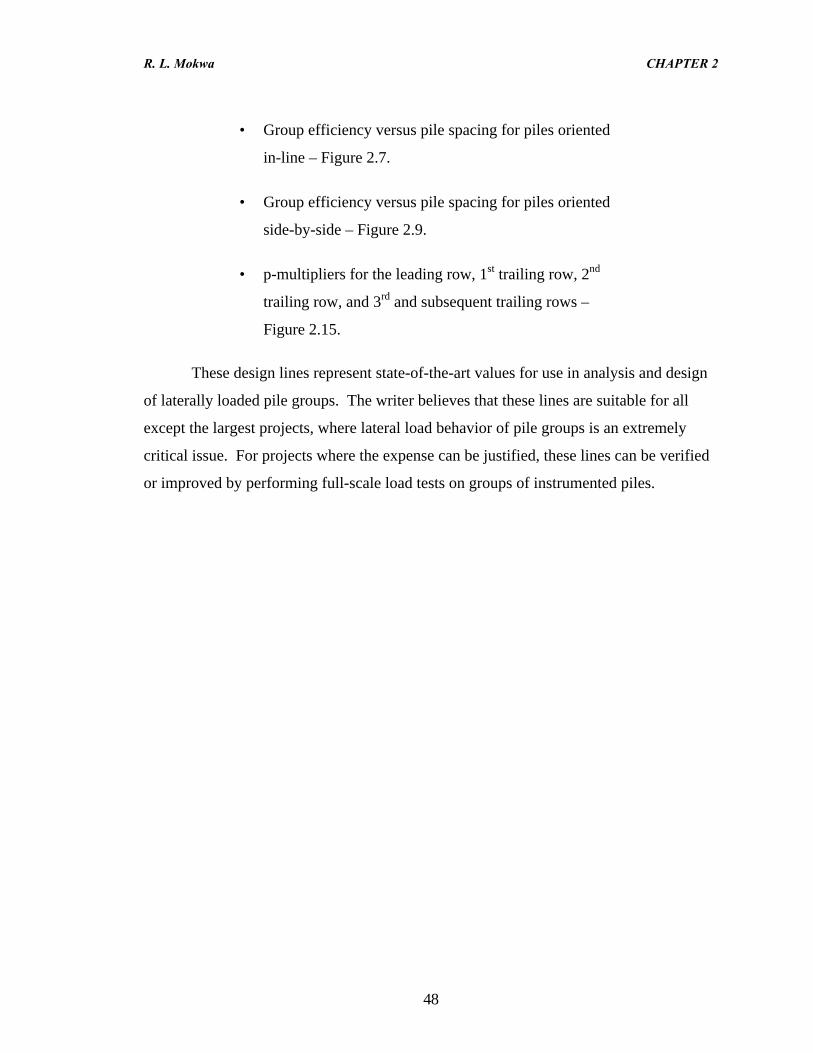
R. L. Mokwa CHAPTER 2
48
• Group efficiency versus pile spacing for piles oriented
in-line – Figure 2.7.
• Group efficiency versus pile spacing for piles oriented
side-by-side – Figure 2.9.
• p-multipliers for the leading row, 1st trailing row, 2nd
trailing row, and 3rd and subsequent trailing rows –
Figure 2.15.
These design lines represent state-of-the-art values for use in analysis and design
of laterally loaded pile groups. The writer believes that these lines are suitable for all
except the largest projects, where lateral load behavior of pile groups is an extremely
critical issue. For projects where the expense can be justified, these lines can be verified
or improved by performing full-scale load tests on groups of instrumented piles.
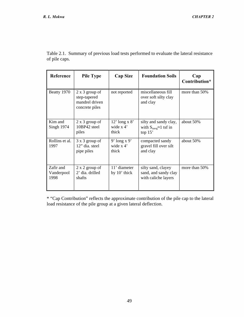
R. L. Mokwa CHAPTER 2
49
Table 2.1. Summary of previous load tests performed to evaluate the lateral resistanceof pile caps.
Reference Pile Type Cap Size Foundation Soils CapContribution*
Beatty 1970 2 x 3 group ofstep-taperedmandrel drivenconcrete piles
not reported miscellaneous fillover soft silty clayand clay
more than 50%
Kim andSingh 1974
2 x 3 group of10BP42 steelpiles
12’ long x 8’wide x 4’thick
silty and sandy clay,with Suavg≈1 tsf intop 15’
about 50%
Rollins et al.1997
3 x 3 group of12” dia. steelpipe piles
9’ long x 9’wide x 4’thick
compacted sandygravel fill over siltand clay
about 50%
Zafir andVanderpool1998
2 x 2 group of2’ dia. drilledshafts
11’ diameterby 10’ thick
silty sand, clayeysand, and sandy claywith caliche layers
more than 50%
* “Cap Contribution” reflects the approximate contribution of the pile cap to the lateralload resistance of the pile group at a given lateral deflection.
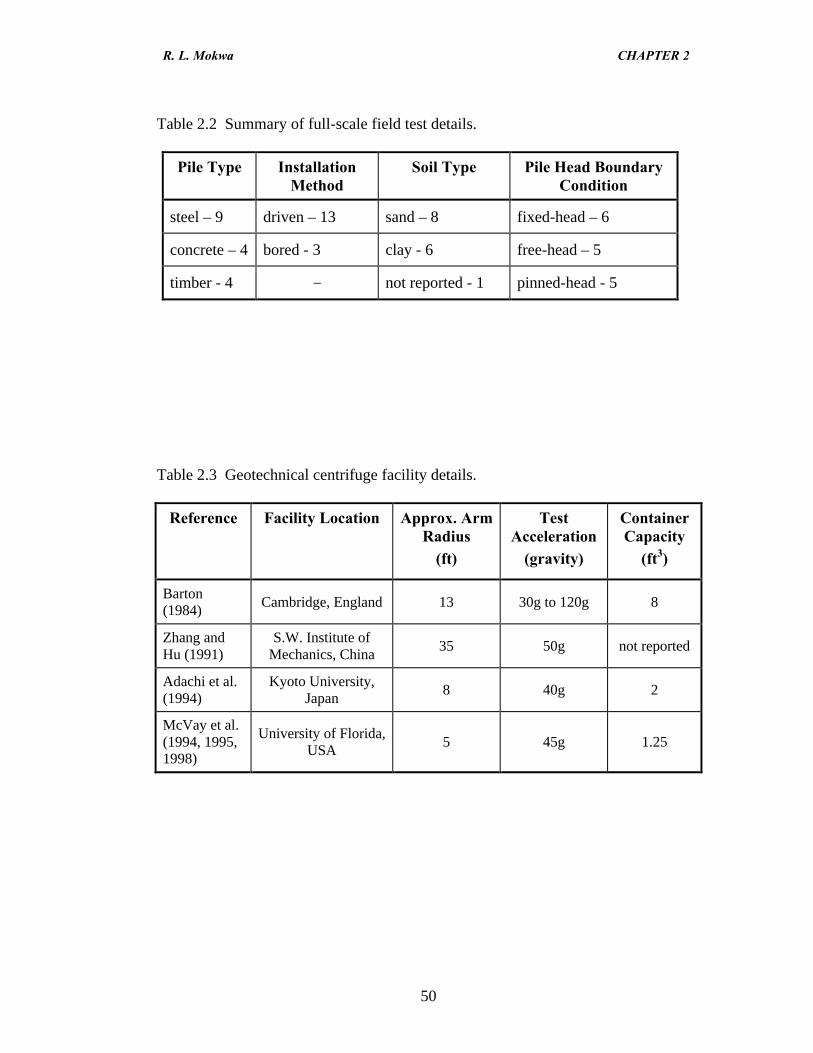
R. L. Mokwa CHAPTER 2
50
Table 2.2 Summary of full-scale field test details.
Pile Type InstallationMethod
Soil Type Pile Head BoundaryCondition
steel – 9 driven – 13 sand – 8 fixed-head – 6
concrete – 4 bored - 3 clay - 6 free-head – 5
timber - 4 − not reported - 1 pinned-head - 5
Table 2.3 Geotechnical centrifuge facility details.
Reference Facility Location Approx. ArmRadius
(ft)
TestAcceleration
(gravity)
ContainerCapacity
(ft3)
Barton(1984) Cambridge, England 13 30g to 120g 8
Zhang andHu (1991)
S.W. Institute ofMechanics, China
35 50g not reported
Adachi et al.(1994)
Kyoto University,Japan
8 40g 2
McVay et al.(1994, 1995,1998)
University of Florida,USA
5 45g 1.25
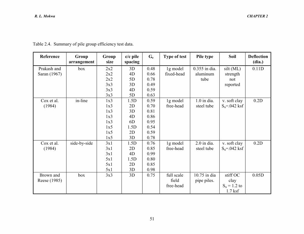
R. L. Mokwa CHAPTER 2
51
Table 2.4. Summary of pile group efficiency test data.
Reference Grouparrangement
Group size
c/c pilespacing
Ge Type of test Pile type Soil Deflection(dia.)
Prakash andSaran (1967)
box 2x22x22x23x33x33x3
3D4D5D3D4D5D
0.480.660.780.490.590.63
1g modelfixed-head
0.355 in dia.aluminum
tube
silt (ML)strength
notreported
0.11D
Cox et al.(1984)
in-line 1x31x31x31x31x31x51x51x5
1.5D2D3D4D6D
1.5D2D3D
0.590.700.810.860.950.540.590.78
1g modelfree-head
1.0 in dia.steel tube
v. soft claySu=.042 ksf
0.2D
Cox et al.(1984)
side-by-side 3x13x13x15x15x15x1
1.5D2D4D
1.5D2D3D
0.760.850.990.800.850.98
1g modelfree-head
2.0 in dia.steel tube
v. soft claySu=.042 ksf
0.2D
Brown andReese (1985)
box 3x3 3D 0.75 full scalefield
free-head
10.75 in diapipe piles.
stiff OCclay
Su = 1.2 to1.7 ksf
0.05D
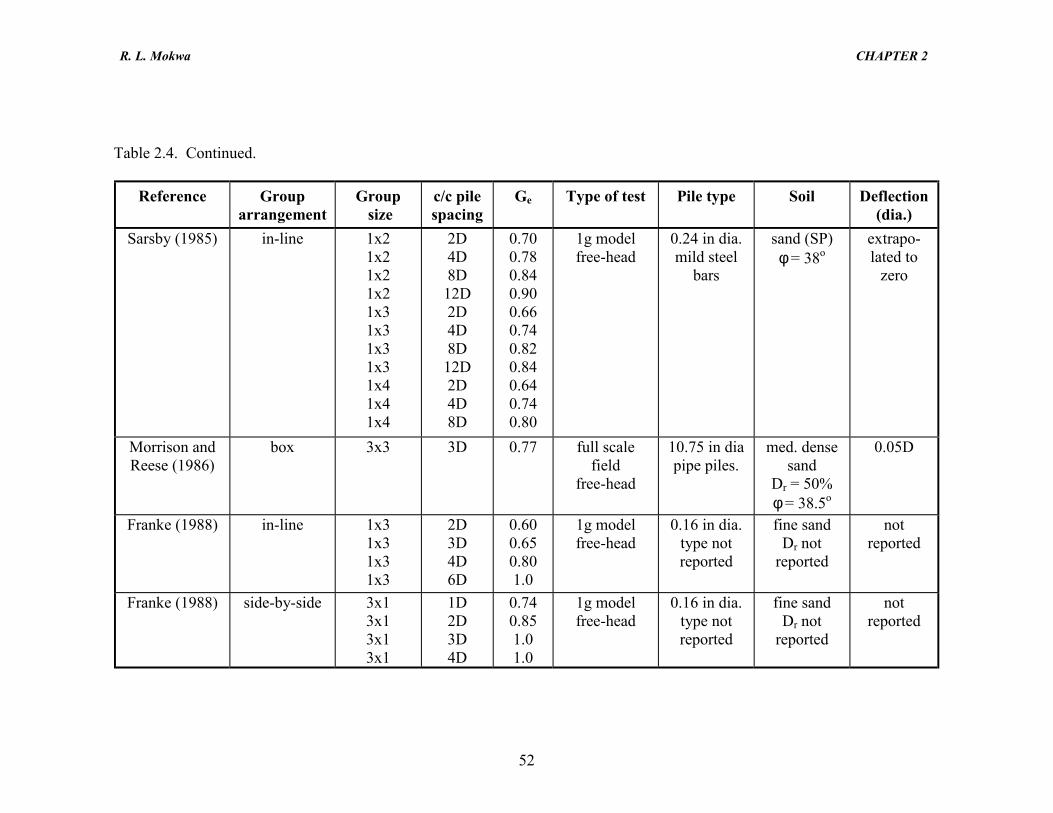
R. L. Mokwa CHAPTER 2
52
Table 2.4. Continued.
Reference Grouparrangement
Group size
c/c pilespacing
Ge Type of test Pile type Soil Deflection(dia.)
Sarsby (1985) in-line 1x21x21x21x21x31x31x31x31x41x41x4
2D4D8D12D2D4D8D12D2D4D8D
0.700.780.840.900.660.740.820.840.640.740.80
1g modelfree-head
0.24 in dia.mild steel
bars
sand (SP)φ = 38o
extrapo-lated to
zero
Morrison andReese (1986)
box 3x3 3D 0.77 full scalefield
free-head
10.75 in diapipe piles.
med. densesand
Dr = 50%φ = 38.5o
0.05D
Franke (1988) in-line 1x31x31x31x3
2D3D4D6D
0.600.650.801.0
1g modelfree-head
0.16 in dia.type notreported
fine sandDr not
reported
notreported
Franke (1988) side-by-side 3x13x13x13x1
1D2D3D4D
0.740.851.01.0
1g modelfree-head
0.16 in dia.type notreported
fine sandDr not
reported
notreported
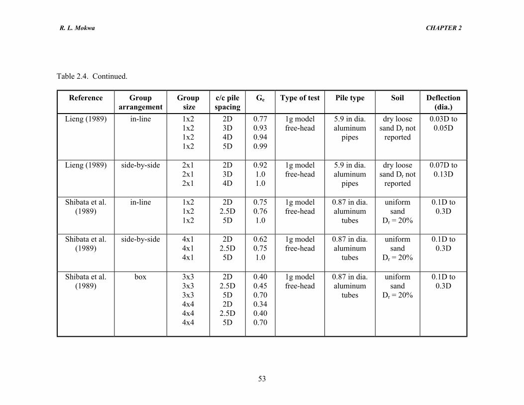
R. L. Mokwa CHAPTER 2
53
Table 2.4. Continued.
Reference Grouparrangement
Group size
c/c pilespacing
Ge Type of test Pile type Soil Deflection(dia.)
Lieng (1989) in-line 1x21x21x21x2
2D3D4D5D
0.770.930.940.99
1g modelfree-head
5.9 in dia.aluminum
pipes
dry loosesand Dr not
reported
0.03D to0.05D
Lieng (1989) side-by-side 2x12x12x1
2D3D4D
0.921.01.0
1g modelfree-head
5.9 in dia.aluminum
pipes
dry loosesand Dr not
reported
0.07D to0.13D
Shibata et al.(1989)
in-line 1x21x21x2
2D2.5D5D
0.750.761.0
1g modelfree-head
0.87 in dia.aluminum
tubes
uniformsand
Dr = 20%
0.1D to0.3D
Shibata et al.(1989)
side-by-side 4x14x14x1
2D2.5D5D
0.620.751.0
1g modelfree-head
0.87 in dia.aluminum
tubes
uniformsand
Dr = 20%
0.1D to0.3D
Shibata et al.(1989)
box 3x33x33x34x44x44x4
2D2.5D5D2D
2.5D5D
0.400.450.700.340.400.70
1g modelfree-head
0.87 in dia.aluminum
tubes
uniformsand
Dr = 20%
0.1D to0.3D
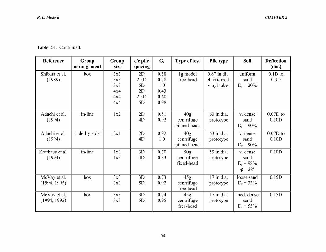
R. L. Mokwa CHAPTER 2
54
Table 2.4. Continued.
Reference Grouparrangement
Group size
c/c pilespacing
Ge Type of test Pile type Soil Deflection(dia.)
Shibata et al.(1989)
box 3x33x33x34x44x44x4
2D2.5D5D2D
2.5D5D
0.580.781.00.430.600.98
1g modelfree-head
0.87 in dia.chloridized-vinyl tubes
uniformsand
Dr = 20%
0.1D to0.3D
Adachi et al.(1994)
in-line 1x2 2D4D
0.810.92
40gcentrifuge
pinned-head
63 in dia.prototype
v. densesand
Dr = 90%
0.07D to0.10D
Adachi et al.(1994)
side-by-side 2x1 2D4D
0.921.0
40gcentrifuge
pinned-head
63 in dia.prototype
v. densesand
Dr = 90%
0.07D to0.10D
Kotthaus et al.(1994)
in-line 1x31x3
3D4D
0.700.83
50gcentrifugefixed-head
59 in dia.prototype
v. densesand
Dr = 98%φ = 38o
0.10D
McVay et al.(1994, 1995)
box 3x33x3
3D5D
0.730.92
45gcentrifugefree-head
17 in dia.prototype
loose sandDr = 33%
0.15D
McVay et al.(1994, 1995)
box 3x33x3
3D5D
0.740.95
45gcentrifugefree-head
17 in dia.prototype
med. densesand
Dr = 55%
0.15D
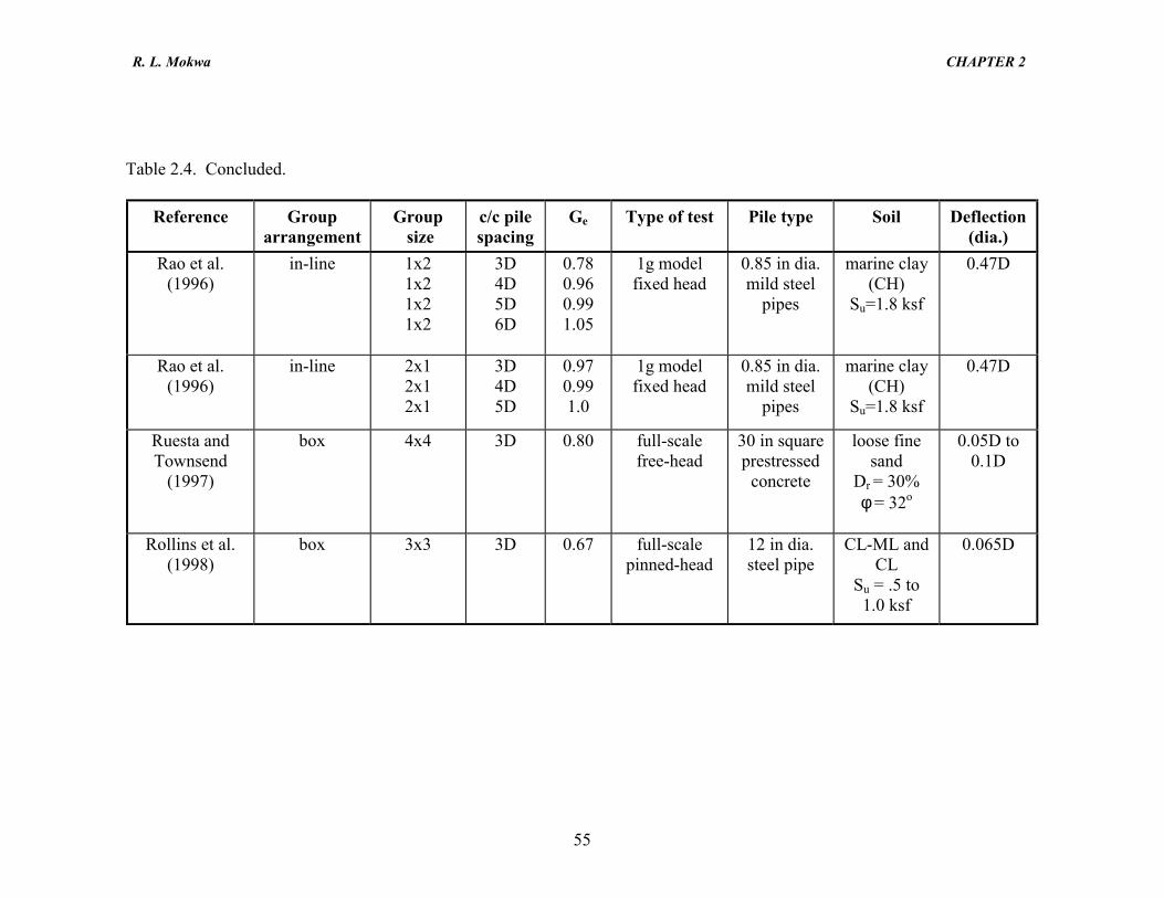
R. L. Mokwa CHAPTER 2
55
Table 2.4. Concluded.
Reference Grouparrangement
Group size
c/c pilespacing
Ge Type of test Pile type Soil Deflection(dia.)
Rao et al.(1996)
in-line 1x21x21x21x2
3D4D5D6D
0.780.960.991.05
1g modelfixed head
0.85 in dia.mild steel
pipes
marine clay(CH)
Su=1.8 ksf
0.47D
Rao et al.(1996)
in-line 2x12x12x1
3D4D5D
0.970.991.0
1g modelfixed head
0.85 in dia.mild steel
pipes
marine clay(CH)
Su=1.8 ksf
0.47D
Ruesta andTownsend
(1997)
box 4x4 3D 0.80 full-scalefree-head
30 in squareprestressed
concrete
loose finesand
Dr = 30%φ = 32o
0.05D to0.1D
Rollins et al.(1998)
box 3x3 3D 0.67 full-scalepinned-head
12 in dia.steel pipe
CL-ML andCL
Su = .5 to1.0 ksf
0.065D
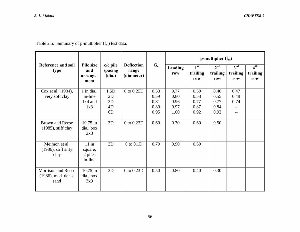
R. L. Mokwa CHAPTER 2
56
Table 2.5. Summary of p-multiplier (fm) test data.
p-multiplier (fm)
Reference and soiltype
Pile sizeand
arrange-ment
c/c pilespacing(dia.)
Deflectionrange
(diameter)
Ge Leadingrow
1st
trailingrow
2nd
trailingrow
3rd
trailingrow
4th
trailingrow
Cox et al. (1984),very soft clay
1 in dia.,in-line
1x4 and1x3
1.5D2D3D4D6D
0 to 0.25D 0.530.590.810.890.95
0.770.800.960.971.00
0.500.530.770.870.92
0.400.550.770.840.92
0.470.490.74
----
Brown and Reese(1985), stiff clay
10.75 india., box
3x3
3D 0 to 0.23D 0.60 0.70 0.60 0.50
Meimon et al.(1986), stiff silty
clay
11 insquare,2 pilesin-line
3D 0 to 0.1D 0.70 0.90 0.50
Morrison and Reese(1986), med. dense
sand
10.75 india., box
3x3
3D 0 to 0.23D 0.50 0.80 0.40 0.30
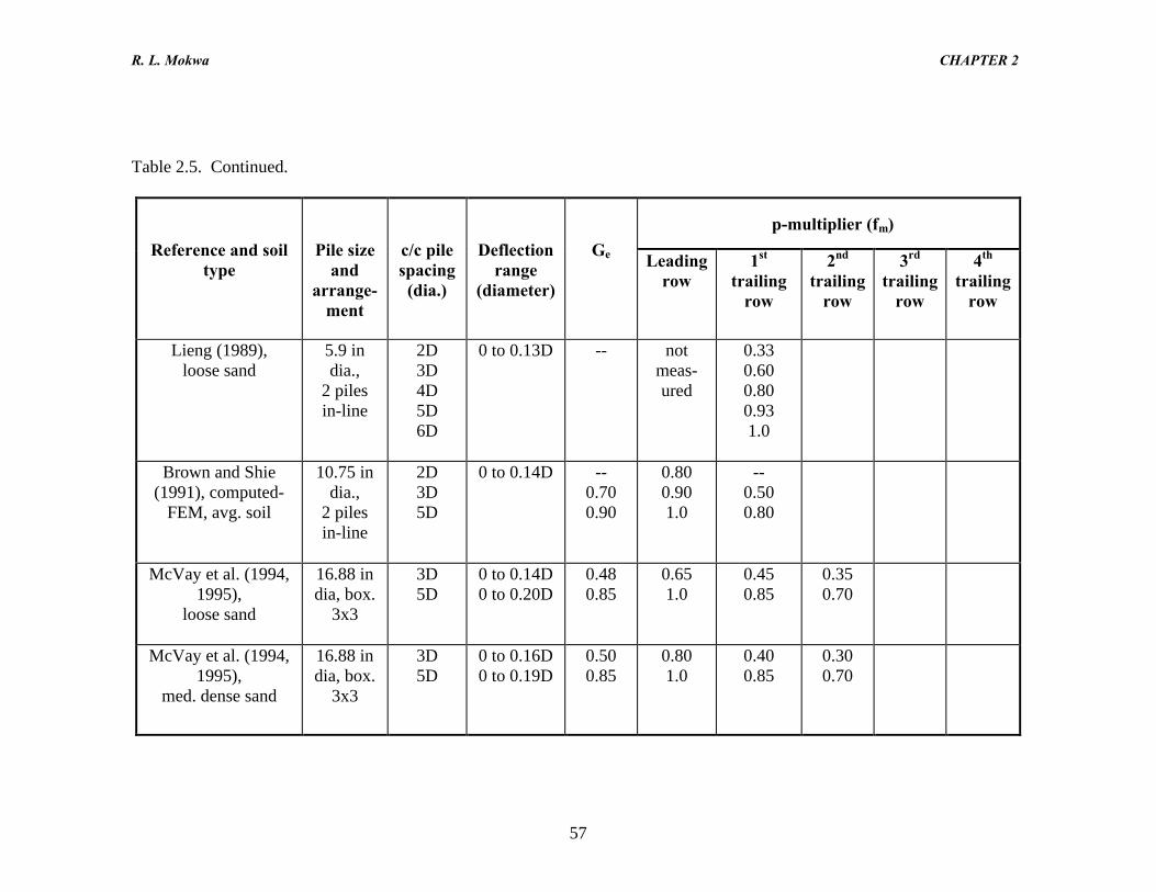
R. L. Mokwa CHAPTER 2
57
Table 2.5. Continued.
p-multiplier (fm)
Reference and soiltype
Pile sizeand
arrange-ment
c/c pilespacing(dia.)
Deflectionrange
(diameter)
Ge Leadingrow
1st
trailingrow
2nd
trailingrow
3rd
trailingrow
4th
trailingrow
Lieng (1989),loose sand
5.9 india.,
2 pilesin-line
2D3D4D5D6D
0 to 0.13D -- notmeas-ured
0.330.600.800.931.0
Brown and Shie(1991), computed-
FEM, avg. soil
10.75 india.,
2 pilesin-line
2D3D5D
0 to 0.14D --0.700.90
0.800.901.0
--0.500.80
McVay et al. (1994,1995),
loose sand
16.88 india, box.
3x3
3D5D
0 to 0.14D0 to 0.20D
0.480.85
0.651.0
0.450.85
0.350.70
McVay et al. (1994,1995),
med. dense sand
16.88 india, box.
3x3
3D5D
0 to 0.16D0 to 0.19D
0.500.85
0.801.0
0.400.85
0.300.70
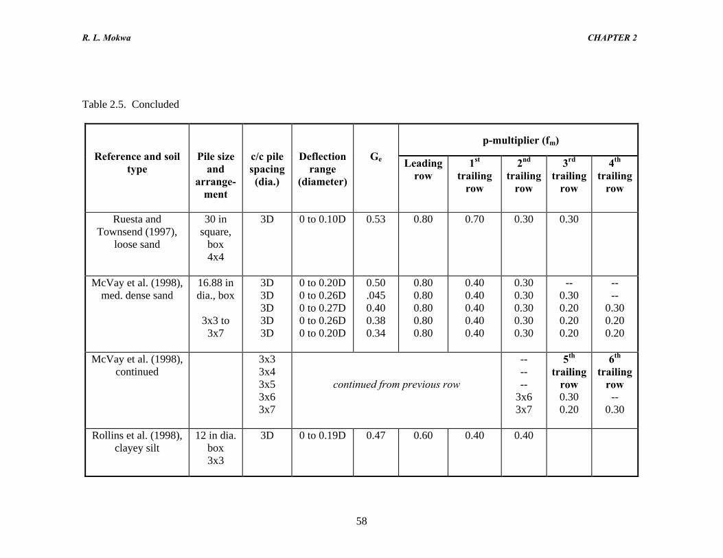
R. L. Mokwa CHAPTER 2
58
Table 2.5. Concluded
p-multiplier (fm)
Reference and soiltype
Pile sizeand
arrange-ment
c/c pilespacing(dia.)
Deflectionrange
(diameter)
Ge Leadingrow
1st
trailingrow
2nd
trailingrow
3rd
trailingrow
4th
trailingrow
Ruesta andTownsend (1997),
loose sand
30 insquare,
box4x4
3D 0 to 0.10D 0.53 0.80 0.70 0.30 0.30
McVay et al. (1998),med. dense sand
16.88 india., box
3x3 to3x7
3D3D3D3D3D
0 to 0.20D0 to 0.26D0 to 0.27D0 to 0.26D0 to 0.20D
0.50.0450.400.380.34
0.800.800.800.800.80
0.400.400.400.400.40
0.300.300.300.300.30
--0.300.200.200.20
----
0.300.200.20
McVay et al. (1998),continued
3x33x43x53x63x7
continued from previous row
------
3x63x7
5th
trailingrow0.300.20
6th
trailingrow
--0.30
Rollins et al. (1998),clayey silt
12 in dia.box3x3
3D 0 to 0.19D 0.47 0.60 0.40 0.40
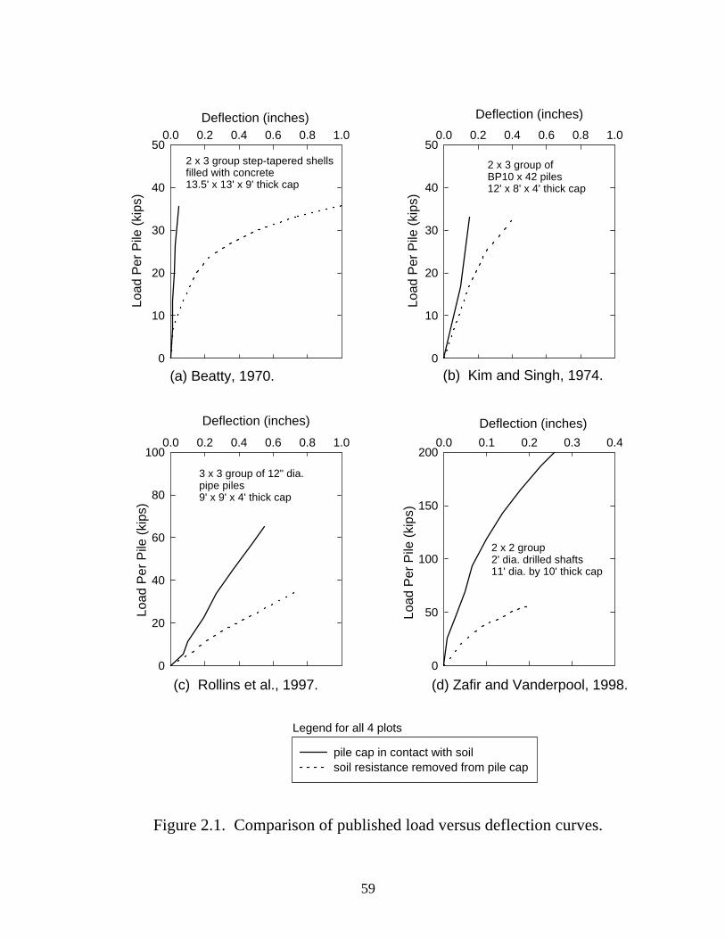
Deflection (inches)
0.0 0.2 0.4 0.6 0.8 1.0
Load
Per
Pile
(ki
ps)
0
20
40
60
80
100
Deflection (inches)
0.0 0.2 0.4 0.6 0.8 1.0
Load
Per
Pile
(ki
ps)
0
10
20
30
40
50
Deflection (inches)0.0 0.2 0.4 0.6 0.8 1.0
Load
Per
Pile
(ki
ps)
0
10
20
30
40
50
pile cap in contact with soilsoil resistance removed from pile cap
Deflection (inches)
0.0 0.1 0.2 0.3 0.4
Load
Per
Pile
(ki
ps)
0
50
100
150
200
3 x 3 group of 12" dia. pipe piles 9' x 9' x 4' thick cap
2 x 3 group of BP10 x 42 piles12' x 8' x 4' thick cap
2 x 3 group step-tapered shellsfilled with concrete13.5' x 13' x 9' thick cap
2 x 2 group 2' dia. drilled shafts11' dia. by 10' thick cap
(b) Kim and Singh, 1974.
(c) Rollins et al., 1997.
(a) Beatty, 1970.
(d) Zafir and Vanderpool, 1998.
Figure 2.1. Comparison of published load versus deflection curves.
59
Legend for all 4 plots
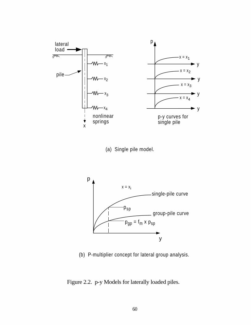
y
y
y
y
p
x = x1
x = x2
x = x3
x = x4
p-y curves forsingle pile
y
p
single-pile curve
group-pile curve
(a) Single pile model.
psp
pgp = fm x psp
(b) P-multiplier concept for lateral group analysis.
x
x1
x2
x3
x4
lateralload
pile
nonlinearsprings
Figure 2.2. p-y Models for laterally loaded piles.
x = xi
60
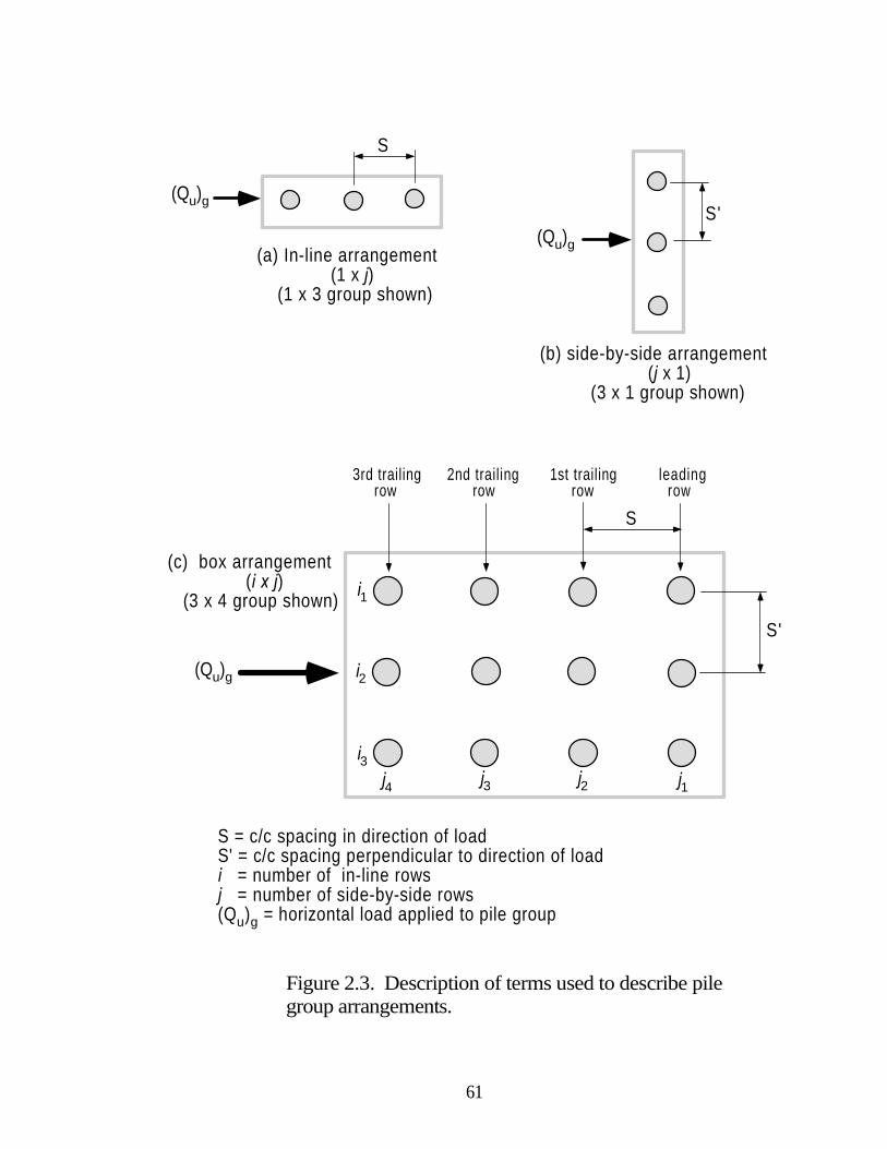
Figure 2.3. Description of terms used to describe pilegroup arrangements.
(a) In-line arrangement (1 x j) (1 x 3 group shown)
(Qu)g
S
(b) side-by-side arrangement (j x 1) (3 x 1 group shown)
(Qu)g
S'
(c) box arrangement (i x j) (3 x 4 group shown)
leading row
1st trailing row
2nd trailing row
3rd trailing row
S'
S
i1
i2
i3j4 j3 j2 j1
S = c/c spacing in direction of loadS' = c/c spacing perpendicular to direction of loadi = number of in-line rowsj = number of side-by-side rows(Qu)g = horizontal load applied to pile group
(Qu)g
61
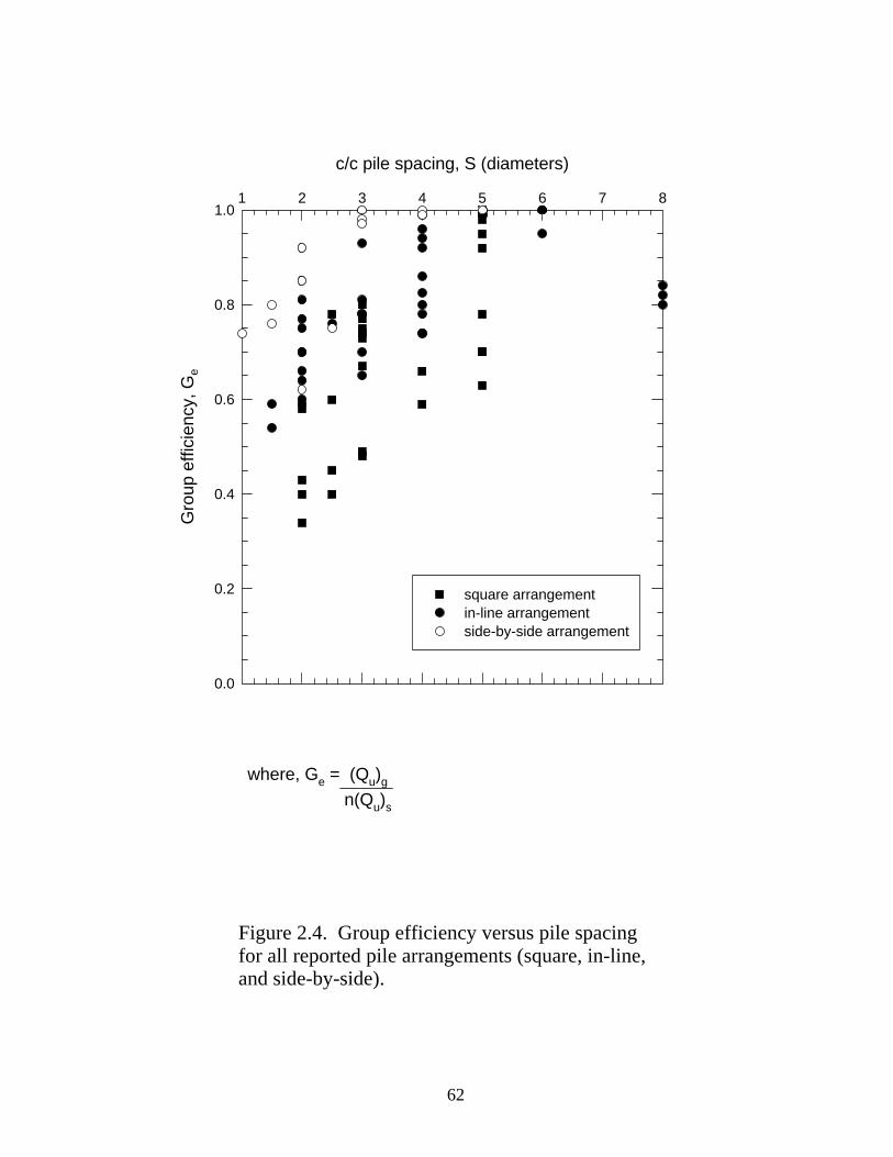
Figure 2.4. Group efficiency versus pile spacingfor all reported pile arrangements (square, in-line,and side-by-side).
c/c pile spacing, S (diameters)
1 2 3 4 5 6 7 8G
roup
effi
cien
cy, G
e
0.0
0.2
0.4
0.6
0.8
1.0
square arrangementin-line arrangementside-by-side arrangement
where, Ge = (Qu)g
n(Qu)s
62
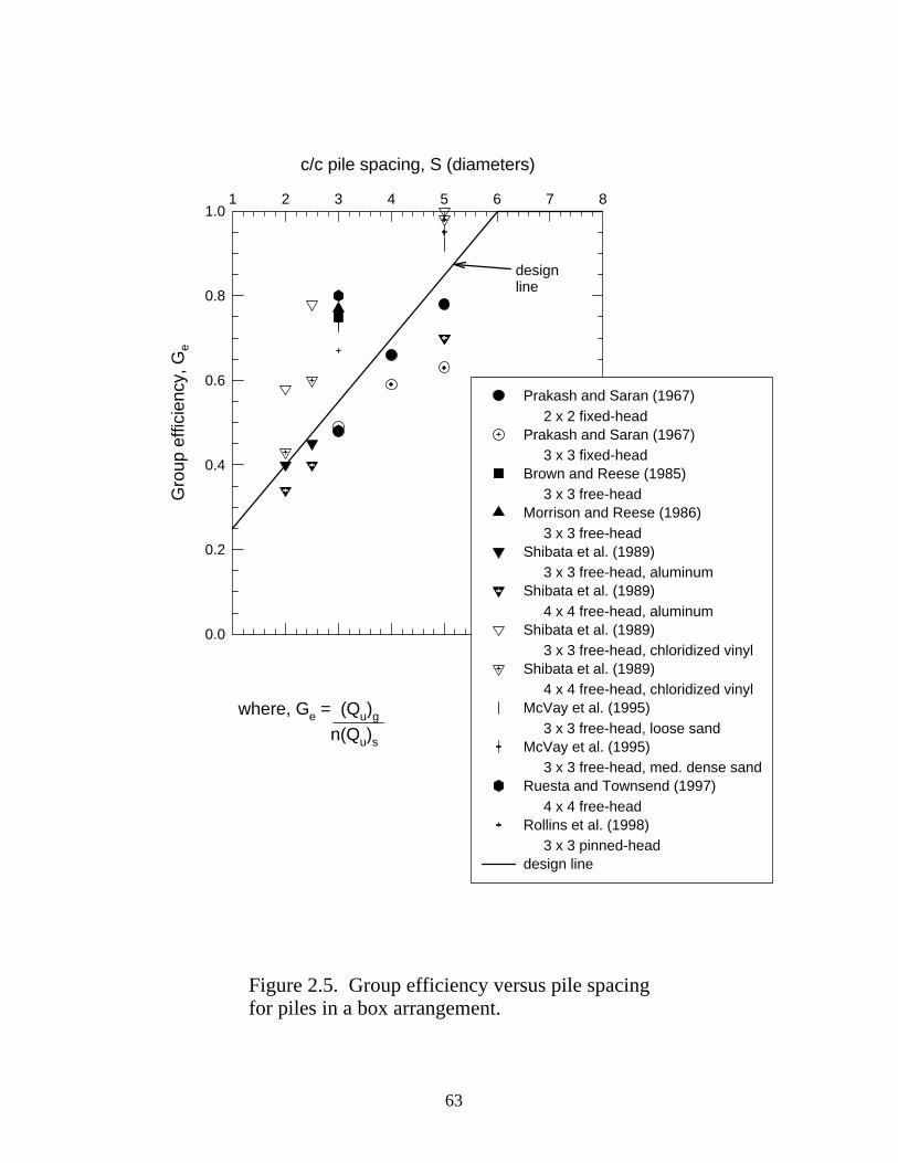
Figure 2.5. Group efficiency versus pile spacingfor piles in a box arrangement.
c/c pile spacing, S (diameters)
1 2 3 4 5 6 7 8G
roup
effi
cien
cy, G
e
0.0
0.2
0.4
0.6
0.8
1.0
Prakash and Saran (1967)
2 x 2 fixed-headPrakash and Saran (1967) 3 x 3 fixed-headBrown and Reese (1985) 3 x 3 free-headMorrison and Reese (1986)
3 x 3 free-headShibata et al. (1989) 3 x 3 free-head, aluminumShibata et al. (1989)
4 x 4 free-head, aluminumShibata et al. (1989) 3 x 3 free-head, chloridized vinylShibata et al. (1989) 4 x 4 free-head, chloridized vinylMcVay et al. (1995)
3 x 3 free-head, loose sandMcVay et al. (1995) 3 x 3 free-head, med. dense sandRuesta and Townsend (1997)
4 x 4 free-headRollins et al. (1998) 3 x 3 pinned-headdesign line
where, Ge = (Qu)g
n(Qu)s
design line
63
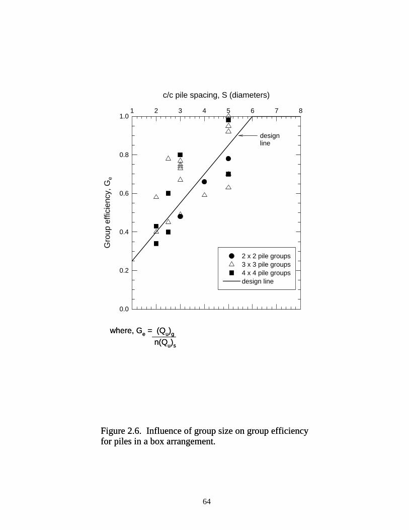
Figure 2.6. Influence of group size on group efficiencyfor piles in a box arrangement.
where, Ge = (Qu)g
n(Qu)s
64
Figure 2.6. Influence of group size on group efficiencyfor piles in a box arrangement.
c/c pile spacing, S (diameters)
1 2 3 4 5 6 7 8G
roup
effi
cien
cy, G
e
0.0
0.2
0.4
0.6
0.8
1.0
2 x 2 pile groups3 x 3 pile groups4 x 4 pile groupsdesign line
where, Ge = (Qu)g
n(Qu)s
designline
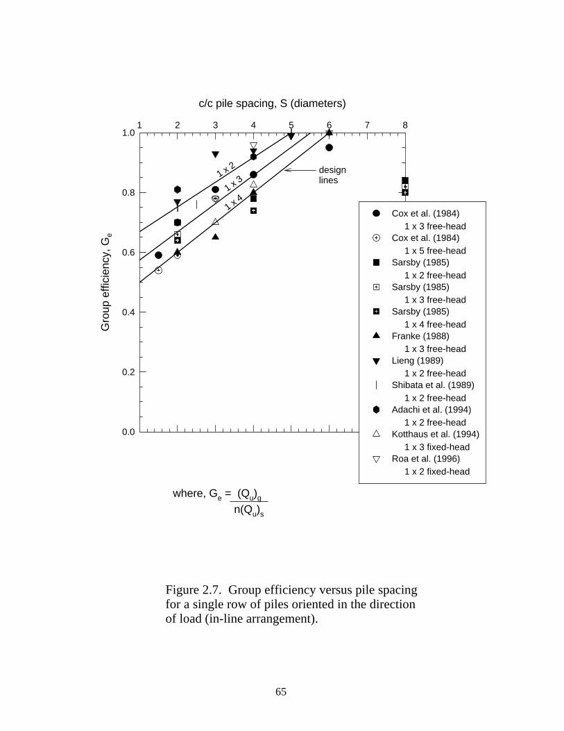
Figure 2.7. Group efficiency versus pile spacingfor a single row of piles oriented in the direction of load (in-line arrangement).
c/c pile spacing, S (diameters)
1 2 3 4 5 6 7 8
Gro
up e
ffici
ency
, Ge
0.0
0.2
0.4
0.6
0.8
1.0
Cox et al. (1984) 1 x 3 free-headCox et al. (1984) 1 x 5 free-headSarsby (1985)
1 x 2 free-headSarsby (1985) 1 x 3 free-headSarsby (1985)
1 x 4 free-headFranke (1988) 1 x 3 free-headLieng (1989) 1 x 2 free-headShibata et al. (1989)
1 x 2 free-headAdachi et al. (1994) 1 x 2 free-headKotthaus et al. (1994)
1 x 3 fixed-headRoa et al. (1996) 1 x 2 fixed-head
where, Ge = (Qu)g
n(Qu)s
1 x 2
1 x 3
1 x 4
designlines
65
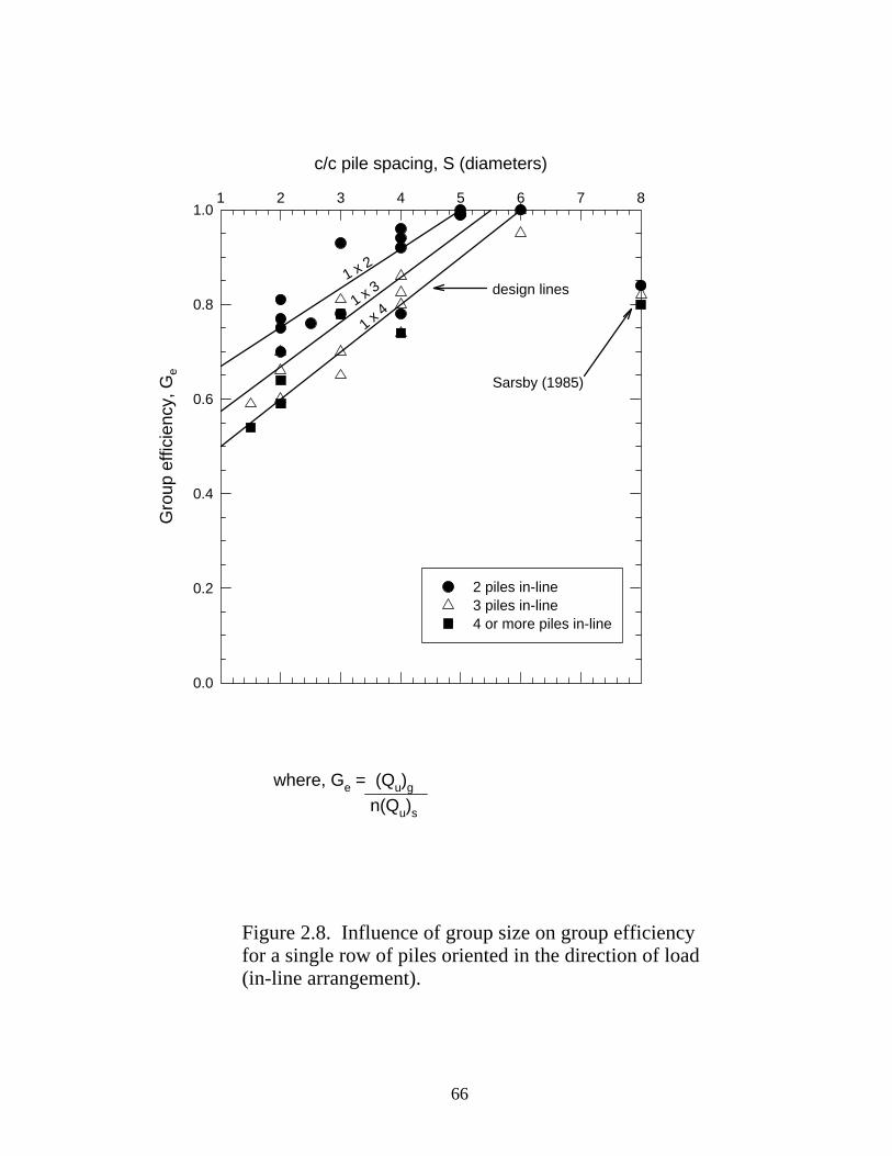
Figure 2.8. Influence of group size on group efficiencyfor a single row of piles oriented in the direction of load(in-line arrangement).
c/c pile spacing, S (diameters)
1 2 3 4 5 6 7 8
Gro
up e
ffici
ency
, Ge
0.0
0.2
0.4
0.6
0.8
1.0
2 piles in-line3 piles in-line4 or more piles in-line
design lines1 x 2
1 x 3
1 x 4
where, Ge = (Qu)g
n(Qu)s
Sarsby (1985)
66
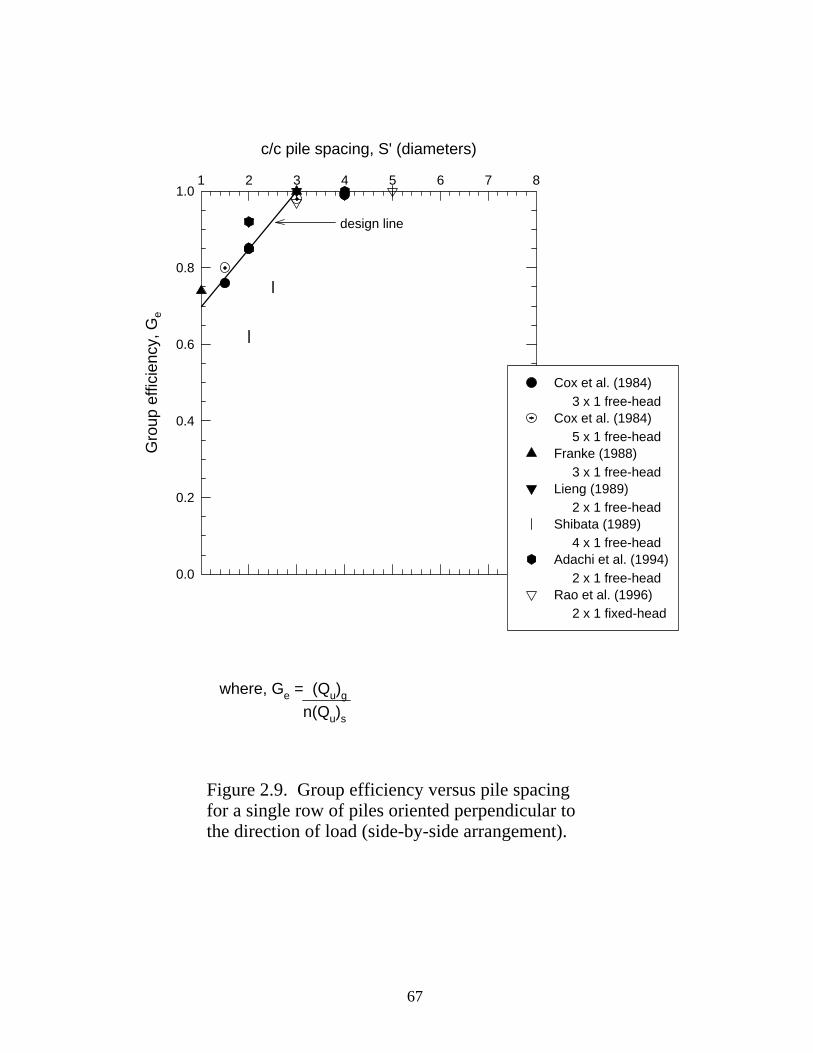
Figure 2.9. Group efficiency versus pile spacingfor a single row of piles oriented perpendicular to the direction of load (side-by-side arrangement).
c/c pile spacing, S' (diameters)
1 2 3 4 5 6 7 8
Gro
up e
ffici
ency
, Ge
0.0
0.2
0.4
0.6
0.8
1.0
Cox et al. (1984)
3 x 1 free-headCox et al. (1984) 5 x 1 free-headFranke (1988)
3 x 1 free-headLieng (1989) 2 x 1 free-headShibata (1989) 4 x 1 free-headAdachi et al. (1994)
2 x 1 free-headRao et al. (1996) 2 x 1 fixed-head
where, Ge = (Qu)g
n(Qu)s
design line
67
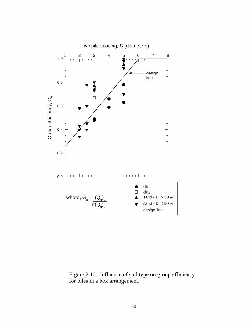
Figure 2.10. Influence of soil type on group efficiencyfor piles in a box arrangement.
c/c pile spacing, S (diameters)
1 2 3 4 5 6 7 8G
roup
effi
cien
cy, G
e
0.0
0.2
0.4
0.6
0.8
1.0
siltclaysand - Dr > 50 %
sand - Dr < 50 %
design line
where, Ge = (Qu)g
n(Qu)s
design line
68
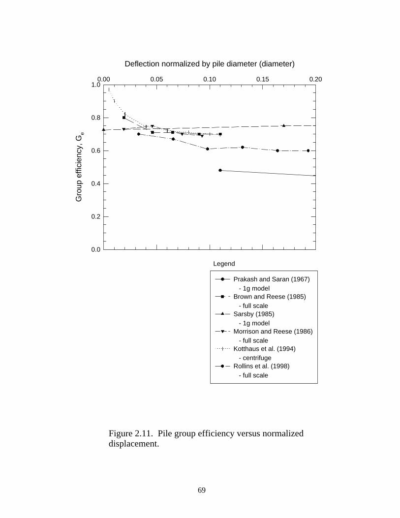
Deflection normalized by pile diameter (diameter)
0.00 0.05 0.10 0.15 0.20G
roup
effi
cien
cy, G
e
0.0
0.2
0.4
0.6
0.8
1.0
Prakash and Saran (1967)
- 1g modelBrown and Reese (1985) - full scaleSarsby (1985)
- 1g modelMorrison and Reese (1986) - full scaleKotthaus et al. (1994) - centrifugeRollins et al. (1998)
- full scale
Figure 2.11. Pile group efficiency versus normalized displacement.
Legend
69
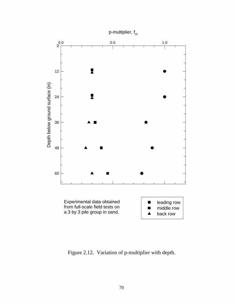
p-multiplier, fm
0.0 0.5 1.0
Dep
th b
elow
gro
und
surf
ace
(in)
0
12
24
36
48
60
leading rowmiddle rowback row
Figure 2.12. Variation of p-multiplier with depth.(From Brown et al., 1988.)
Experimental data obtainedfrom full-scale field tests ona 3 by 3 pile group in sand.
70
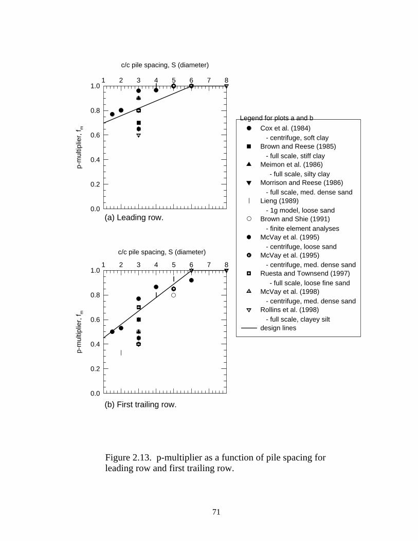
c/c pile spacing, S (diameter)
1 2 3 4 5 6 7 8
p-m
ultip
lier,
f m
0.0
0.2
0.4
0.6
0.8
1.0
(b) First trailing row.
(a) Leading row.
Figure 2.13. p-multiplier as a function of pile spacing for leading row and first trailing row.
c/c pile spacing, S (diameter)
1 2 3 4 5 6 7 8p-
mul
tiplie
r, f m
0.0
0.2
0.4
0.6
0.8
1.0
Cox et al. (1984)
- centrifuge, soft clayBrown and Reese (1985) - full scale, stiff clayMeimon et al. (1986) - full scale, silty clayMorrison and Reese (1986)
- full scale, med. dense sandLieng (1989) - 1g model, loose sandBrown and Shie (1991)
- finite element analysesMcVay et al. (1995) - centrifuge, loose sandMcVay et al. (1995) - centrifuge, med. dense sandRuesta and Townsend (1997)
- full scale, loose fine sandMcVay et al. (1998) - centrifuge, med. dense sandRollins et al. (1998)
- full scale, clayey siltdesign lines
Legend for plots a and b
71
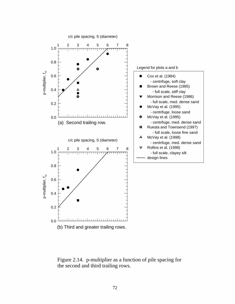
c/c pile spacing, S (diameter)
1 2 3 4 5 6 7 8
p-m
ultip
lier,
f m
0.0
0.2
0.4
0.6
0.8
1.0
(a) Second trailing row.
(b) Third and greater trailing rows.
Figure 2.14. p-multiplier as a function of pile spacing forthe second and third trailing rows.
c/c pile spacing, S (diameter)
1 2 3 4 5 6 7 8p-
mul
tiplie
r, f m
0.0
0.2
0.4
0.6
0.8
1.0
Cox et al. (1984) - centrifuge, soft clayBrown and Reese (1985)
- full scale, stiff clayMorrison and Reese (1986) - full scale, med. dense sandMcVay et al. (1995)
- centrifuge, loose sandMcVay et al. (1995) - centrifuge, med. dense sandRuesta and Townsend (1997) - full scale, loose fine sandMcVay et al. (1998)
- centrifuge, med. dense sandRollins et al. (1998) - full scale, clayey siltdesign lines
Legend for plots a and b
72
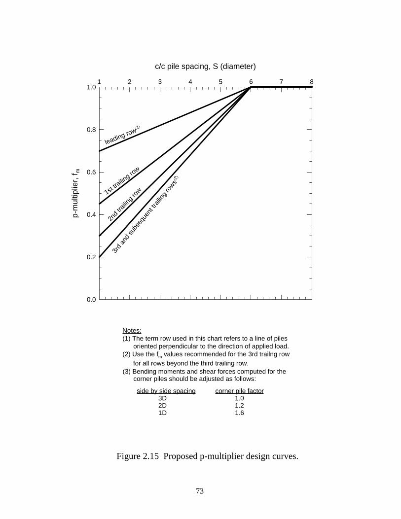
Figure 2.15 Proposed p-multiplier design curves.
c/c pile spacing, S (diameter)
1 2 3 4 5 6 7 8p-
mul
tiplie
r, f m
0.0
0.2
0.4
0.6
0.8
1.0
leading row(1)
1st tra
iling ro
w
2nd
trailin
g ro
w
3rd
and
subs
eque
nt tr
ailin
g ro
ws(2
)
Notes:(1) The term row used in this chart refers to a line of piles oriented perpendicular to the direction of applied load. (2) Use the fm values recommended for the 3rd trailng row
for all rows beyond the third trailing row.
73
(3) Bending moments and shear forces computed for the corner piles should be adjusted as follows: side by side spacing corner pile factor
3D 1.0 2D 1.2 1D 1.6
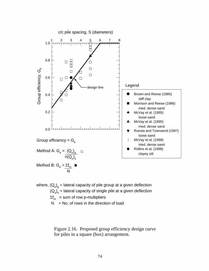
Figure 2.16. Proposed group efficiency design curvefor piles in a square (box) arrangement.
c/c pile spacing, S (diameters)
1 2 3 4 5 6 7 8G
roup
effi
cien
cy, G
e
0.0
0.2
0.4
0.6
0.8
1.0
Brown and Reese (1985)
stiff clayMorrison and Reese (1986)
med. dense sandMcVay et al. (1995) loose sandMcVay et al. (1995)
med. dense sandRuesta and Townsend (1997) loose sandMcVay et al. (1998) med. dense sandRollins et al. (1998)
clayey silt
Group efficiency = Ge
Method A: Ge = (Qu)g
n(Qu)s
Method B: Ge = Σfm N
where, (Qu)g = lateral capacity of pile group at a given deflection
(Qu)s = lateral capacity of single pile at a given deflection
Σfm = sum of row p-multipliers
N = No. of rows in the direction of load
Legenddesign line
74