Embed Size (px)
Citation preview

Mechanics of Soft Materials Volokh 2010
MECHANICS OF SOFT MATERIALS
K. Y. Volokh
Faculty of Civil and Environmental Engineering
Technion – Israel Institute of Technology
Contents
1. Tensors 2
2. Kinematics 16
3. Balance laws 28
4. Isotropic elasticity 37
5. Anisotropic elasticity 49
6. Viscoelasticity 56
7. Chemo-mechanical coupling 64
8. Electro-mechanical coupling 71
9. Appendix 79
Mechanics of Soft Materials Volokh 2010 2
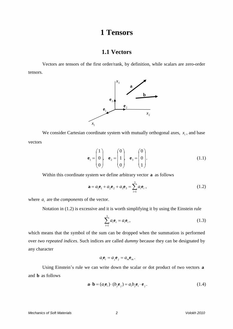
1 Tensors
1.1 Vectors
Vectors are tensors of the first order/rank, by definition, while scalars are zero-order
tensors.
We consider Cartesian coordinate system with mutually orthogonal axes, ix , and base
vectors
1
0
0
,
0
1
0
,
0
0
1
321 eee . (1.1)
Within this coordinate system we define arbitrary vector a as follows
3
1
332211
i
iiaaaa eeeea , (1.2)
where ia are the components of the vector.
Notation in (1.2) is excessive and it is worth simplifying it by using the Einstein rule
ii
i
ii aa ee
3
1
, (1.3)
which means that the symbol of the sum can be dropped when the summation is performed
over two repeated indices. Such indices are called dummy because they can be designated by
any character
mmjjii aaa eee .
Using Einstein’s rule we can write down the scalar or dot product of two vectors a
and b as follows
jijijjii baba eeeeba )()( . (1.4)
1x
2x
3x
1e
3e
2e
a
b
Mechanics of Soft Materials Volokh 2010 3
The scalar product of base vectors is zero for different base vectors and one for the
same vector
ijjiji
ji
,0
,1ee , (1.5)
where we introduced the (Leopold) Kronecker delta for short notation.
Substituting (1.5) in (1.4) we have
332211 bababababababa jjiiijjijiji
ij
eeba , (1.6)
where
iiiiijj bbbbb 332211 . (1.7)
By using the dot product of base vector ie with vector a we find ia
iijjjijjjii aaaa eeeeae )( . (1.8)
The Kronecker delta was introduced through the scalar products of the Cartesian base
vectors. It is also very convenient to introduce the permutation (Tulio Levi-Civita) symbol by
using triple product of base vectors
ijkkji
ijk
ijk
ijk
...,0
132;213;321,1
312;231;123,1
)( eee . (1.9)
The permutation symbol allows us to write the components of the vector product in a
short way
kjijkkjkjikkjjiiii bababac
ijk
)}({)}(){()( eeeeeebaece
c
. (1.10)
It is important that there is no summation over index i in (1.10). Such index is called
free. Computing (1.10) for varying i we get
122133113223321 ,, babacbabacbabac . (1.11)
1.2 Second-order tensors
To define a second-order tensor we introduce dyadic or tensor product, , of base
vectors
000
000
001
001
0
0
1
1111
Teeee ,
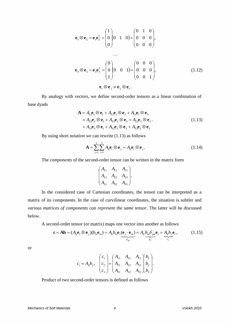
Mechanics of Soft Materials Volokh 2010 4
000
000
010
010
0
0
1
2121
Teeee ,
…
100
000
000
100
1
0
0
3333
Teeee , (1.12)
ijji eeee .
By analogy with vectors, we define second-order tensors as a linear combination of
base dyads
333323321331
322322221221
311321121111
eeeeee
eeeeee
eeeeeeA
AAA
AAA
AAA
. (1.13)
By using short notation we can rewrite (1.13) as follows
jiij
j i
jiij AA eeeeA
3
1
3
1
. (1.14)
The components of the second-order tensor can be written in the matrix form
333231
232221
131211
AAA
AAA
AAA
.
In the considered case of Cartesian coordinates, the tensor can be interpreted as a
matrix of its components. In the case of curvilinear coordinates, the situation is subtler and
various matrices of components can represent the same tensor. The latter will be discussed
below.
A second-order tensor (or matrix) maps one vector into another as follows
i
c
jiji
b
jmmijmjimijmmjiij
ijjm
bAbAbAbA eeeeeeeeAbc
)())(( , (1.15)
or
3
2
1
333231
232221
131211
3
2
1
,
b
b
b
AAA
AAA
AAA
c
c
c
bAc jiji .
Product of two second-order tensors is defined as follows

Mechanics of Soft Materials Volokh 2010 5
ni
F
jnijnijmmnij
nimjmnijnmmnjiij
in
jm
DADA
DADA
eeee
eeeeeeeeADF
)())((
, (1.16)
or
333231
232221
131211
333231
232221
131211
333231
232221
131211
,
DDD
DDD
DDD
AAA
AAA
AAA
FFF
FFF
FFF
DAF jnijin .
Double dot product of two tensors is a scalar
333312121111 ....
)()()(:)(:
DADADADADA
DADA
mjmj
D
jnmn
A
imij
njmimnijnmmnjiij
mjmj
jnim
eeeeeeeeDA
. (1.17)
By using the double dot product we can calculate components of a second-order
tensor as follows
ijnjmimnnmmnjiji AAA
jnim
)()()(:: eeeeeeeeAee . (1.18)
Since the second-order tensor can be interpreted as a matrix then all subsequent
definitions for tensors are analogous to the matrix definitions. For example, the second-order
identity tensor is defined as
332211 eeeeeeee1 jiij , (1.19)
and it enjoys the remarkable property
A1AA1 . (1.20)
The transposed second-order tensor is
jijiijij
T
jiij
T AAA eeeeeeA )( . (1.21)
It allows us to additively decompose any second-order tensor into symmetric and
skew (anti)-symmetric parts
T
skew
T
skew
T
sym
T
symskewsym AAAAAAAAAAA )(2
1,)(
2
1, . (1.22)
The inverse second order tensor, 1A , is defined through the identity
1AAAA 11 . (1.23)

Mechanics of Soft Materials Volokh 2010 6
Finally, we consider the eigenproblem for a symmetric second-order tensor TAA .
The eigenvalue (principal value) and the eigenvector (principal direction) n of the tensor
are defined by the following equation
nAn . (1.24)
The eigenproblem defines the principal directions of tensor A where vector n is
mapped into itself scaled by factor . We rewrite the eigenproblem by moving all terms onto
the left hand side
0n1A )( , (1.25)
or
0
0
0
3
2
1
333231
232221
131211
n
n
n
AAA
AAA
AAA
.
This equation possesses a nontrivial solution when the determinant of the coefficient
matrix is singular
0)()()()det( 321
23 AAA1A III . (1.26)
Here the principal invariants of tensor A have been introduced
AA tr)( 3322111 AAAI , (1.27)
)}(tr)tr{(2
1)( 22
2 AAA I , (1.28)
AA det)(3 I . (1.29)
Since tensor A is symmetric then all roots of (1.26) , 321 ,, , are real and it is
possible to find three mutually orthogonal principal directions corresponding to the roots. The
unit vectors in principal directions, )3()2()1( ,, nnn , obey the orthonormality conditions
ij
ji )()(nn . (1.30)
Now tensor A can enjoy the spectral decomposition based on the solution of the
eigenproblem
)3()3(
3
)2()2(
2
)1()1(
1 nnnnnnA , (1.31)
if 321 , or
1nnA 2
)1()1(
21 )( , (1.32)
if 321 , or
1A 1 . (1.33)
Mechanics of Soft Materials Volokh 2010 7
if 321 .
Based on the spectral decomposition it is convenient to introduce the logarithm and
the square root of a symmetric positive definite tensor, 0i ,
3
1
)()()(lnlnk
kk
k nnA , (1.34)
3
1
)()(
k
kk
k nnA . (1.35)
The spectral decomposition also allows us to calculate the principal invariants simply
3211 )( AI , (1.36)
3231212 )( AI , (1.37)
3213 )( AI . (1.38)
Finally, we derive the useful Cayley-Hamilton formula pre-multiplying (1.26) with
)(in and accounting for )()( ia
i
iannA
0A1AAAAA )()()( 321
23 III . (1.39)
1.3 Tensor functions
Tensors can be arguments of functions: )(Af ; )( ijAf ; )(Af ; )( ijm Af ; )(AF ;
)( ijmn AF . Let us calculate a differential of a scalar function f with respect to tensor
argument A
ij
ij
dAA
fdf
. (1.40)
Here the components of the tensor increment can be written as (see (1.18))
Aee ddA jiij : ,
and, consequently, (1.40) takes form
AA
Aee df
dA
fdf ji
ij
::
, (1.41)
where the derivative with respect to the second-order tensor has been defined
ji
ijA
ffee
A
. (1.42)
Analogously, it is possible to define the derivative of a second-order tensor
Mechanics of Soft Materials Volokh 2010 8
jinm
C
ij
mnji
ij
mnij
B
A
Beeeeee
A
B
AC
. (1.43)
This is the fourth-order tensor, which is formed by a combination of base tetrads
jinm eeee that can be interpreted, by analogy with dyads, as tables (matrices) in 4D
space.
The double dot product of the fourth- and second- order tensors is defined as follows
nm
D
ijmnijljkinmklmnij
lkkljinmmnij
mnjlik
BCBC
BC
eeeeeeee
eeeeeeBCD
)()(
)(:)(:
. (1.44)
As an example let us differentiate a second-order tensor with respect to itself
jinmnjmijinm
ij
mn
A
Aeeeeeeee
A
A
. (1.45)
In the case of symmetric tensor 2/)( TAAA the symmetry should be preserved
in the derivative
jinmmjninjmi
T
eeeeA
AA
A
A
)(
2
1)(
2
1 . (1.46)
Further important formulas are obtained by differentiating the principal invariants of
TAA
1eeeeA
A
jikjkiji
ij
kk
ij
A
AI
)(1 , (1.47)
A1AeeA
A
)(
)(
2
1)(1
2 IA
AAAAIji
ij
nmmnllkk . (1.48)
The derivative of the third invariant AA det)(3 I is less trivial and we start with
calculating the increment of it with the help of (1.26)
)}()()(1{det
))1(det(det)det(
1
3
1
2
1
1
eigenvaluetensor
1
AAAAAAA
1AAAAA
dIdIdI
dd
. (1.49)
Ignoring higher-order terms in (1.49) we have
AAAAAAAAAA
AA
ddId T
dT
:)(detdet)(detdet)det(
:
1
1
, (1.50)
and, consequently,

Mechanics of Soft Materials Volokh 2010 9
TI
AA
A
A
A
A)(det
)(det)(3 . (1.51)
1.4 Tensor analysis
We turn to tensor analysis and define the following differential operators for vectors
and second-order tensors in Cartesian coordinates
i
ixe
x
grad , (1.52)
ij
i
j
i
i x
a
xeee
a
x
aa
grad , (1.53)
i
iij
i
j
i
i x
a
x
a
x
eee
aadiv , (1.54)
2
1
1
23
1
3
3
12
3
2
2
31
curl
x
a
x
a
x
a
x
a
x
a
x
a
x
a
x
a
x i
j
kkij
i
j
ji
i
i
eee
eeea
ea
, (1.55)
3
3
33
2
32
1
31
2
3
23
2
22
1
21
1
3
13
2
12
1
11
)(div
e
e
e
eeeeeA
A
x
A
x
A
x
A
x
A
x
A
x
A
x
A
x
A
x
A
x
A
x
A
xm
n
mninm
i
mni
i
. (1.56)
Now we refresh our memories concerning the divergence theorem (Gauss, Green, and
Ostrogradskii) which is an important tool for transforming volume and area integrals. Its
simplest version in one-dimensional case is the famous Newton-Leibnitz rule
)()()()()()1()()1( ayanbybnaybydxdx
dyb
a
.
In a three-dimensional case we can write
)(an )(bn x
a b

Mechanics of Soft Materials Volokh 2010 01
ydAndV
x
yi
i
. (1.57)
The powerful generalization of this formula is
dAnB
dAnBdAnBdAnB
dVx
BdV
x
BdV
x
BdV
x
B
jij
iii
iii
j
ij
332211
3
3
2
2
1
1
, (1.58)
or, shortly,
dAdV BnBdiv . (1.59)
Of course, the second-order tensor B can be replaced by scalar b or vector b
dAbdVb ngrad , (1.60)
dAdV nbbdiv . (1.61)
Another useful formula is due to Stokes who related the contour integral over curve l
to surface A built on it
dAd nbxb )(curl , (1.62)
where xd is the infinitesimal element of the curve l .
1.5 Curvilinear coordinates
Some problems are easier to solve in curvilinear rather than Cartesian coordinates.
We consider curvilinear coordinates ),,( 321 which can be defined through the Cartesian
A
V
n
n
A
l

Mechanics of Soft Materials Volokh 2010 00
coordinates ),,( 321 xxx and vice versa. For example, in the case of cylindrical coordinates we
have
zr 321 ;; , (1.63)
zxrxrx 321 ;sin;cos , (1.64)
3
1
22
2
2
1 ;arctan; xzx
xxxr . (1.65)
We define the natural (co-variant) base vectors in curvilinear coordinates
ji
j
i
xes
, (1.66)
which take the following form in cylindrical coordinates
333
22
11
2133
22
11
2133
22
11
cossin
sincos
eeees
eeeees
eeeees
z
x
z
x
z
x
rrxxx
r
x
r
x
r
x
z
r
. (1.67)
We also define the dual (contra-variant) base vectors
j
j
ii
xes
, (1.68)
which take the following form in cylindrical coordinates
33
3
2
2
1
1
213
3
2
2
1
1
213
3
2
2
1
1
cossin
sincos
eeees
eeeees
eeeees
x
z
x
z
x
z
rrxxx
x
r
x
r
x
r
z
r
. (1.69)
1x
2x
3x
r
z
1e
3e
2e
rg
zg
g

Mechanics of Soft Materials Volokh 2010 02
The natural and dual base vectors are mutually orthogonal
ji
ji
x
x
x
x
x
xi
j
m
j
i
mmn
n
j
i
mn
n
j
mi
mj
i,0
,1
eess . (1.70)
Now vectors and tensors may have various representations in curvilinear coordinates
i
ii
i aa ssa , (1.71)
j
ij
i
j
i
i
j
ji
ijji
ij AAAA ssssssssA .
. , (1.72)
where iia sa are contra-variant components; and iia sa are co-variant components;
)(: jiijA ssA are contra-variant components; )(: jiijA ssA are co-variant
components; and )(:. j
i
j
iA ssA and )(:. j
ii
jA ssA are mixed components.
In the case where the base vectors are mutually orthogonal it is possible to normalize
them. For example, in the case of the cylindrical coordinates we have
1
0
0
,
0
cos
sin
,
0
sin
cos
z
z
z
zzr
r
r
rr
s
s
s
sg
s
s
s
sg
s
s
s
sg
. (1.73)
The normalized base vectors allow introducing the so-called physical components of
vectors and tensors with the same units
zzrr aaa ggga , (1.74)
zzzzzzrzzr
zzrr
zrrzrrrrrr
AAA
AAA
AAA
gggggg
gggggg
ggggggA
. (1.75)
Now we calculate differential operators in curvilinear coordinates
j
ji
i
j
ji
i
j
xxs
ae
ae
aa
s
grad , (1.76)
j
j
ji
i
j
i
i
j
xx
as
ae
aea
s
curl , (1.77)
j
ji
i
j
ji
i
j
xxs
Be
Be
BB
s
div . (1.78)
In the case of cylindrical coordinates we have, for example,

Mechanics of Soft Materials Volokh 2010 03
zr
zr
zrr
zr
ggg
sss
(...)(...)1(...)
(...)(...)(...)grad(...)
. (1.79)
In calculating the derivatives of vectors and tensors one should not forget that the
natural and dual and physical base vectors depend on coordinates! In the considered case of
cylindrical coordinates we have the following derivatives of the physical base vectors
0g
0g
0g
0g
gg
gg
0g
0g
0g
zzz
rrr
zr
zr
r
zr
;;
;;
;;
. (1.80)
Besides the considered cylindrical coordinates it is useful to list the basic relationships
for spherical coordinates
321 ;;r , (1.81)
cos;sinsin;sincos 321 rxrxrx , (1.82)
1
2
2
3
2
2
2
1
32
3
2
2
2
1 arctan;arccos;x
x
xxx
xxxxr
, (1.83)
0
cos
sin
,
sin
sincos
coscos
,
cos
sinsin
sincos
gggr , (1.84)
ggg
(...)
sin
1(...)1(...)grad(...)
rrrr , (1.85)
1x
2x
3x
r
1e
3e
2e
rg
g g
Mechanics of Soft Materials Volokh 2010 04
cossin;cos;sin
;;
;;
ggg
gg
gg
0g
gg
gg
0g
0g
0g
rr
rr
r
rrr
. (1.86)
1.6 Homework
1. Prove:
tptntm
kpknkm
spsnsm
mnpskt
det , (1.87)
tnkptpknsnpskt , (1.88)
tptptptkkptpkkskpskt 23 , (1.89)
62 ttsktskt . (1.90)
2. Prove (1.20).
3. Prove for second-order tensors A, B:
pktjsistpijk AAA6
1det A , (1.91)
A
Adet
1det 1 , (1.92)
111)( ABAB , (1.93)
TTT AAA )()( 11 . (1.94)
4. Prove (1.37).
5. Prove (1.48).
6. Prove for second-order tensors A, B:
BABA :)(tr 1 T . (1.95)
7. Prove for scalar :
0gradcurl . (1.96)
8. Prove for vector a :
0curldiv a . (1.97)
9. Prove (1.84).
10. Prove (1.85).

Mechanics of Soft Materials Volokh 2010 05
11. Prove (1.86).

Mechanics of Soft Materials Volokh 2010 06
2 Kinematics
2.1 Deformation gradient
We consider deformation of a body shown in its reference and current states. The law
of motion of material points, i.e. infinitesimal material volumes, is defined by
),( txyy , (2.1)
where x and y are the reference and current positions of the point. It is usually convenient,
yet not necessary, to assume that the reference state is the initial one: )0,( txyx .
If we consider x as an independent variable then we follow motion of a material
point that was fixed at x in the reference configuration. Such description is called referential
or material or Lagrangean. If, alternatively, we consider y as an independent variable then
we follow motion of various material points passing through y in the current configuration.
The latter description is called spatial or Eulerian. The Eulerian description is preferable
when the evolution of continuum boundaries is known beforehand like in many problems of
fluid mechanics while the Lagrangean description is preferable when the evolution of
continuum boundaries is not known beforehand like in many problems of solid mechanics.
An infinitesimal material fiber at points x and y before and after deformation
accordingly can be described by the linear mapping (transformation)
xFy dd , (2.2)
where
1x
2x
3x
1e
3e
2e
0
x
uxd
y
yd
Mechanics of Soft Materials Volokh 2010 07
ji
j
i
x
yee
x
yF
(2.3)
is the tensor of deformation gradient. This tensor is related to two configurations
simultaneously and because of that it is called two-point.
Alternatively, we can use the displacement vector, xyu , to get
H1x
uxF
)(, (2.4)
where
ji
j
i
x
uee
x
uH
(2.5)
is the displacement gradient tensor.
It is possible to calculate any deformation when the deformation gradient is known.
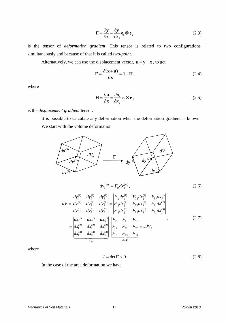
We start with the volume deformation
)()( m
jij
m
i dxFdy , (2.6)
0
det
332313
322212
312111
)3(
3
)3(
2
)3(
1
)2(
3
)2(
2
)2(
1
)1(
3
)1(
2
)1(
1
)3(
3
)3(
2
)3(
1
)2(
3
)2(
2
)2(
1
)1(
3
)1(
2
)1(
1
)3(
3
)3(
2
)3(
1
)2(
3
)2(
2
)2(
1
)1(
3
)1(
2
)1(
1
0
JdV
FFF
FFF
FFF
dxdxdx
dxdxdx
dxdxdx
dxFdxFdxF
dxFdxFdxF
dxFdxFdxF
dydydy
dydydy
dydydy
dV
dV
jjjjjj
jjjjjj
jjjjjj
F
, (2.7)
where
0det FJ . (2.8)
In the case of the area deformation we have
)1(xd
)2(xd
)3(xd
0dVdV
F
)1(yd
)2(yd)3(
yd

Mechanics of Soft Materials Volokh 2010 08
xn ddAdV 000 , (2.9)
xFnyn ddAddAdV . (2.10)
Using (2.7) we derive
xnxFn ddAJddA 00 , (2.11)
0)( 00 xnnF ddAJdAT . (2.12)
Since xd is arbitrary we can write the Nanson formula
00dAJdA TnFn
. (2.13)
Now we define the fiber stretch in direction 1; mm
Fmx
xF
x
ym
d
d
d
d)( . (2.14)
We can also define the change of angle between two fibers by using stretches as
follows, for example,
0dAdA
0dV
xd
0n
dV
nyd
xdm yd
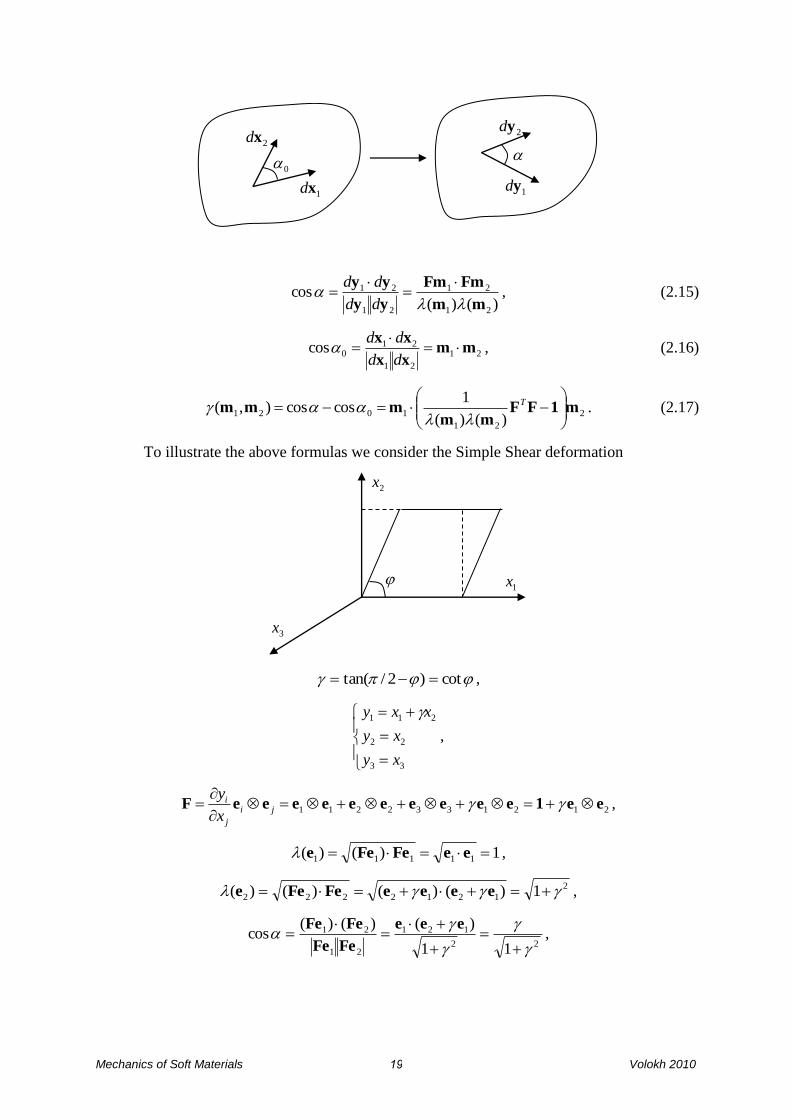
Mechanics of Soft Materials Volokh 2010 09
)()(
cos21
21
21
21
mm
FmFm
yy
yy
dd
dd, (2.15)
21
21
210cos mm
xx
xx
dd
dd , (2.16)
2
21
1021)()(
1coscos),( m1FF
mmmmm
T
. (2.17)
To illustrate the above formulas we consider the Simple Shear deformation
cot)2/tan( ,
33
22
211
xy
xy
xxy
,
2121332211 ee1eeeeeeeeeeF
ji
j
i
x
y,
1)()( 11111 eeFeFee ,
2
1212222 1)()()()( eeeeFeFee ,
22
121
21
21
11
)()()(cos
eee
FeFe
FeFe,
3x
2x
1x
2xd
1xd
0
2yd
1yd

Mechanics of Soft Materials Volokh 2010 21
2/2/)arccos(cos
2)sin/(cos1
sin/cosarccos
21arccos2/
220
.
2.2 Polar decomposition of deformation gradient
Let us square the expression for stretch (2.14) and rewrite it as follows
CmmFmFmFmFmm T)()()(2 , (2.18)
where
FFCT (2.19)
is the right Cauchy-Green tensor.
In the case where direction m is the principal direction of tensor C we have
i
i
i
iiii )()()()()(2 )( mmCmmm , (2.20)
where i and )(im are the eigenvalues and eigenvectors of C.
The above equation means that eigenvalues of the right Cauchy-Green tensor are
equal to the squared stretches in principal directions. Thus we can write the following
spectral decomposition of C in the form
)3()3(2
3
)2()2(2
2
)1()1(2
1 mmmmmmC . (2.21)
Now we define the right stretch tensor as the square root of the right Cauchy-Green
tensor
)3()3(
3
)2()2(
2
)1()1(
1 mmmmmmCU , (2.22)
where all principal stretches are nonnegative.
We assume now that any deformation can be multiplicatively decomposed into stretch
and some additional deformation which we designate R
RUF , (2.23)
which is called the polar decomposition of the deformation gradient and, consequently,
1 FUR . (2.24)
Let us analyze properties of R. First, we observe that it is orthogonal
1UUUUUUUUFFUFUFURRU
112111
2
)()( TTTTTTT. (2.25)
Orthogonal tensors do not change lengths
xxxxRRxxRxRyyy dddddddddd T )()( . (2.26)

Mechanics of Soft Materials Volokh 2010 20
Besides, we observe
1det
det
det
det
det
det
det
)det(
det
detdet
det
detdet
2
U
U
U
U
U
C
U
FF
U
FF
U
FR
TT
. (2.27)
Equations (2.25) and (2.27) mean that R is the proper orthogonal or rotation tensor.
Finally we notice that the meaning of the polar decomposition, RUF , is the
successive stretch and rotation.
It is possible, of course, to change the order of stretch and rotation
VRF , (2.28)
where V is called the left stretch tensor.
By direct computation we have
TTTVRURFRFRV 1 , (2.29)
which means that the left stretch tensor is the rotated right stretch tensor, and consequently
they have the same eigenvalues – principal stretches, while their principal directions are
different.
With account of the spectral decomposition of U we have
)3()3(
3
)2()2(
2
)1()1(
1 nnnnnnV , (2.30)
where
)()()()( iiiiRmRmnn . (2.31)
To clarify the meaning of the principal directions of V we square the tensor as follows
BFFRURURURRURV TTTT ))((2 , (2.32)
xd
xRdR
xF
xVR
xRUy
d
d
dd
U
VRRUF
R
V
xUd

Mechanics of Soft Materials Volokh 2010 22
)3()3(2
3
)2()2(2
2
)1()1(2
1 nnnnnnB , (2.33)
where B is the left Cauchy-Green tensor, which principal directions coincide with the
principal directions of V while the principal values of B are squared principal stretches.
Unfortunately, we cannot directly write the relations between the directions of the
principal stretches in the reference and current configurations because these directions are not
defined uniquely and can always be changed to the opposite sign! However, we can define
the principal directions uniquely by the following procedure. Assume, for example, that the
principal directions in the reference configuration, )(im , are uniquely chosen then we
calculate the principal directions in the current configuration as follows
)()( iiRmn . (2.34)
Of course, we could start with the current configuration otherwise.
Finally, we can calculate the spectral decomposition of the deformation gradient
)3()3(
3
)2()2(
2
)1()1(
1
)3()3(
3
)2()2(
2
)1()1(
1
mnmnmn
mRmmRmmRmRUF
. (2.35)
Let us consider the following deformation (Marsden and Hughes, 1983) as a
numerical example
33
22
211
2
3
xy
xy
xxy
.
In this case we have
100
053
033
,
100
020
013
CF ,
1
0
0
,1,
0
1
3
2
1,2,
0
3
1
2
1,6 )3(
3
)2(
2
)1(
1 mmm ,
6400
03333
033331
64
1,
2200
033133
03333
22
1 1UU ,
200
03113
01331
2
1,
2200
03131
01331
22
1VR .

Mechanics of Soft Materials Volokh 2010 23
2.3 Strains
The strain measures can be introduced in various ways. We start with 1D measures
for the change of the length of a material fiber.
We can introduce the engineering strain
10
0
L
LLE , (2.36)
or the logarithmic strain
lnln0
0
L
L
L
dLL
L
L , (2.37)
or the Green strain
)1(2
1
2
2
2
0
2
0
2
L
LLG . (2.38)
In order to generalize 1D to 3D strains we assume that formulas (2.36)-(2.38) are
valid in the principal directions of the reference configuration. In this case, the 3D strain
tensors take forms
1Ummε
3
1
)()()1(i
ii
iE , (2.39)
Ummε ln)(ln3
1
)()( i
ii
iL , (2.40)
)(2
1)1(
2
1 23
1
)()(21Ummε
i
ii
iG . (2.41)
The Green strain tensor is the most popular and it can be rewritten by dropping the
suffix
)(2
1)(
2
1)(
2
1)(
2
1 2HHHH1FF1C1Uε
TTT . (2.42)
2.4 Motion
Velocity and acceleration are defined as material time derivatives accordingly
0L L

Mechanics of Soft Materials Volokh 2010 24
uuxyxyv ),( tdt
d, (2.43)
vv
a dt
d. (2.44)
When the Eulerian or spatial description is used it is necessary to use the chain rule
for differentiation of any function, )),(( ttf y :
vy
y
yy
f
t
f
t
f
t
fttf
dt
df)),(( , (2.45)
vy
vvv
va
tdt
d . (2.46)
Another important kinematic quantity is the velocity gradient, L ,
LFx
y
y
v
x
v
x
y
x
yF
dt
d, (2.47)
1
FF
y
vL . (2.48)
It can be decomposed into symmetric and skew symmetric parts
)(2
1),(
2
1, TT
LLωLLdωdL , (2.49)
where d and ω are the deformation rate and the spin (vorticity) tensors accordingly.
2.5* Deformation gradient in curvilinear coordinates
We consider the deformation gradient in curvilinear coordinates. To be specific we
choose the deformation law in cylindrical coordinates before },,{ ZR and after },,{ zr
deformation:
),,();,,();,,( ZRzzZRZRrr . (2.50)
To treat this deformation we introduce the natural curvilinear base vectors for the
reference and current configurations accordingly
1
0
0
;
0
cos
sin
;
0
sin
cos
ZR GGG
, (2.51)
1
0
0
;
0
cos
sin
;
0
sin
cos
zr ggg
. (2.52)

Mechanics of Soft Materials Volokh 2010 25
Now the deformation gradient can be written as follows
ZRZRR
Gy
Gy
Gy
F
1, (2.53)
where
zr
z
y
r
y
r
y
zr
zrr
yyy
gg
ggggg
eeey
eee
33
2211
)cos(sinsin)sin(coscos
332211
. (2.54)
We have with account of constantzg
ZzZr
Zr
zr
r
RzRr
Rr
Zzrzr
Rzr
Z
z
Z
r
Z
r
R
z
R
r
R
r
R
z
Rr
R
r
Z
zr
R
zr
R
zr
GgGg
Gg
GgGg
Gg
GgGg
Gg
Ggg
Ggg
Ggg
F
)()()(
, (2.55)
where
ggggg
ggggg
ggggg
ZZ
z
zZZ
r
rZ
z
z
r
r
RR
z
zRR
r
rR
rrrr
rrrr
rrrr
. (2.56)
Finally, we have
ZzzRz
ZR
ZrrRr
Z
z
R
z
R
z
Z
r
R
r
R
r
Z
r
R
r
R
r
GgGgGg
GgGgGg
GgGgGgF
. (2.57)
Alternatively, we can express the deformation gradient through the displacement
vector related to the initial configuration. In the latter, case we have to write
ZR ZR GGx , (2.58)
ZZRR uuu GGGu . (2.59)
These vectors can be written with respect to the coordinates in the current
configuration as follows

Mechanics of Soft Materials Volokh 2010 26
z
x
z
x
r
x
r
zr
ggxggxggxx
ˆˆˆ
)()()(ˆ
, (2.60)
z
u
z
u
r
u
r
zr
gguggugguu
ˆˆˆ
)()()(ˆ
, (2.61)
or
gxx ˆ , (2.62)
guu ˆ , (2.63)
where
zzrr ggggggg (2.64)
is the metric tensor in the current configuration. It is the identity tensor in curvilinear
coordinates.
Now we have
)()()())(()ˆˆ(
HGgHGguxx
y
y
g
x
uxg
x
ux
x
yF
, (2.65)
where
0y
g
, (2.66)
Hx
u
, (2.67)
and
ZZRR GGGGGGGx
x
(2.68)
is the metric tensor in the reference configuration.
2.6 Homework
1. Find principal directions and stretches for the following deformation law
33
212
211
)1(
)1(
xy
xxy
xxy
, (2.69)
where constant .
2. Make the polar decomposition of the deformation gradient for the deformation law
presented in (2.69).

Mechanics of Soft Materials Volokh 2010 27
3. Calculate the Cartesian components of the Green strain for the deformation law presented
in (2.69).
4. Read Section 2.5.
5. Prove (2.66).
6. Prove (2.68).

Mechanics of Soft Materials Volokh 2010 28
3 Balance laws
3.1 Material time derivatives of integrals
We start with the computation of the material time derivative of a volume integral.
For the field quantity )),(( tty over a “moving” region, )(tV , whose configuration depends
on time t , we have the following formula (regarding the integral as an infinite sum)
dVt
dVdt
d
dVy
v
y
v
y
v
dt
d
dvdydydydvdydydydvdydydydt
d
tdytdytdydt
dtdV
dt
d
))(div(
)div(
)(
)(
))()()(()(
3
3
2
2
1
1
321321321321
321
v
v
, (3.1)
where the last equality is obtained as follows
i
i
i
ii
ii
ii
i y
v
ty
vv
yty
v
t
y
ytdt
d
)(div
v .
3.2 Mass conservation
The law of mass conservation can be written as follows
constant dVm , (3.2)
where is mass density.
Differentiating (3.2) with respect to time we have
0))div(()div(
dV
tdV
dt
ddV
dt
d
dt
dmvv
. (3.3)
Since the equality is obeyed for any volume we can localize the condition for the
infinitesimal volume
0)div(div
vv
tdt
d. (3.4)
3.3 Balance of linear momentum
Mechanics of Soft Materials Volokh 2010 29
We start with the balance of linear momentum for a volumeless particle – Newton's
law –
pv )(mdt
d, (3.5)
where vm is the linear momentum and p is the force resultant.
By analogy with Newton’s law Euler considered the balance of the linear momentum
for a continuum volume V bounded by surface A
dAdVdVdt
dtbv , (3.6)
where b is the body force per unit mass and t is the surface force or traction per unit area.
Let us localize the Euler law. First, differentiating the left-hand side of (3.6) we get
dVdt
ddV
dt
d)div
)(( vv
vv
. (3.7)
Then we rewrite the Euler law in the form
dAdV tf , (3.8)
where
vvv
bf div)(
dt
d (3.9)
is the generalized body force.
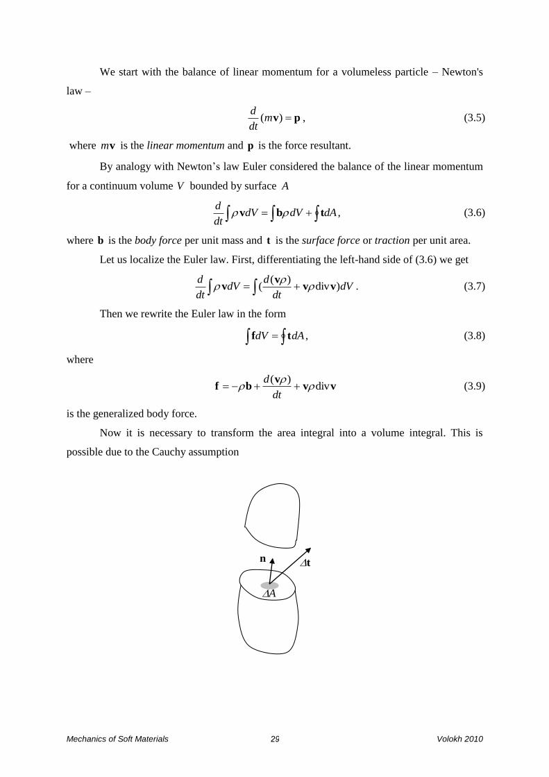
Now it is necessary to transform the area integral into a volume integral. This is
possible due to the Cauchy assumption
n t
A
Mechanics of Soft Materials Volokh 2010 31
),(lim0
nytt
t AA
. (3.10)
The first corollary of the Cauchy assumption is the Newton law of action and
counteraction.
For every part of the body we have
*)(
*)(
22
11
dAdAdV
dAdAdV
nttf
nttf. (3.11)
Summing the equalities we get
*)]()([ dAdAdV ntnttf . (3.12)
Substitution of (3.8) in (3.12) yields
0ntnt *)]()([ dA . (3.13)
This equality is correct for any surface; consequently, we can localize it and get the
third Newton law
)()( ntnt . (3.14)
The second corollary of the Cauchy assumption is the appearance of the stress tensor.
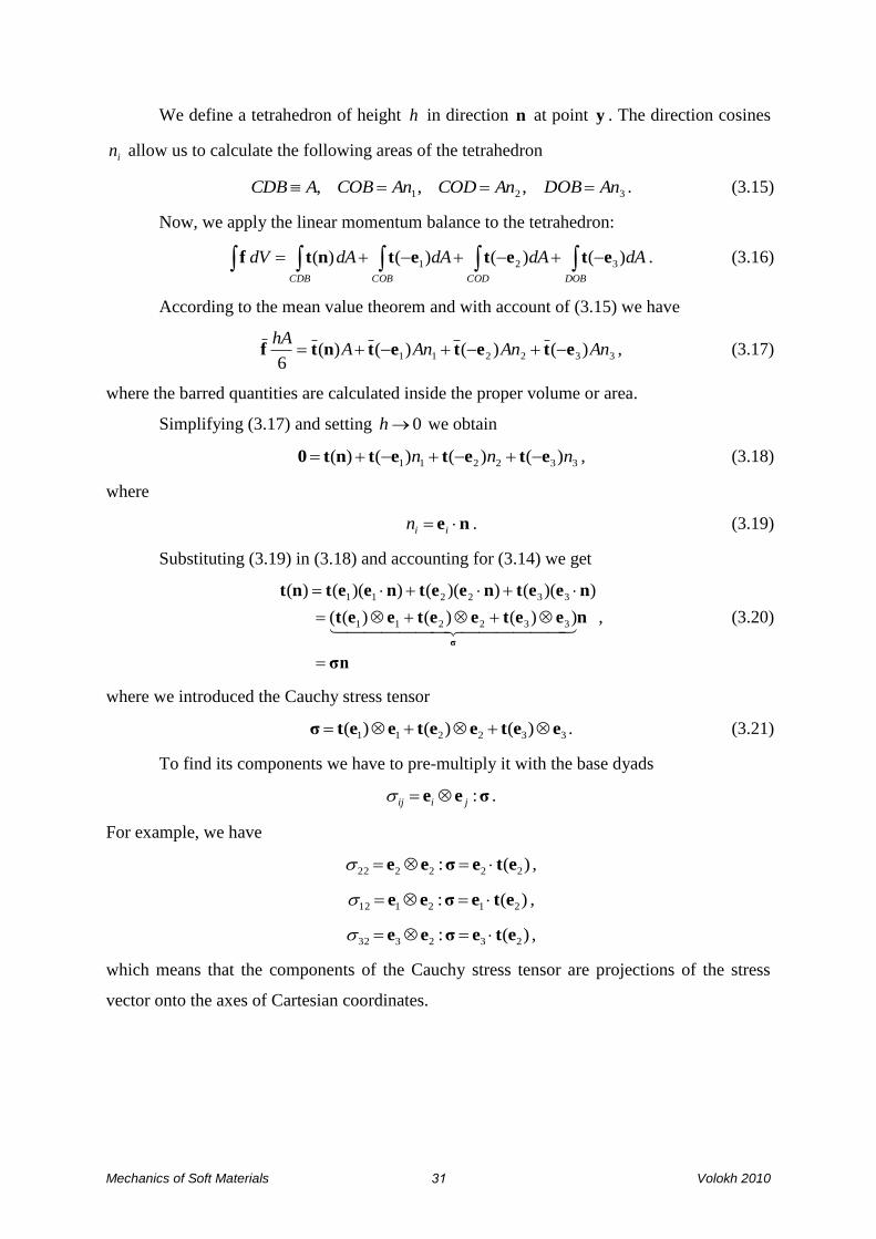
)(nt
n
O B
D
C
1e 2e
3e
3y
1y
2y
h
1A
2A
*A
2V
1V
n
n
Mechanics of Soft Materials Volokh 2010 30
We define a tetrahedron of height h in direction n at point y . The direction cosines
in allow us to calculate the following areas of the tetrahedron
321 ,,, AnDOBAnCODAnCOBACDB . (3.15)
Now, we apply the linear momentum balance to the tetrahedron:
DOBCODCOBCDB
dAdAdAdAdV )()()()( 321 etetetntf . (3.16)
According to the mean value theorem and with account of (3.15) we have
332211 )()()()(6
AnAnAnAhA
etetetntf , (3.17)
where the barred quantities are calculated inside the proper volume or area.
Simplifying (3.17) and setting 0h we obtain
332211 )()()()( nnn etetetnt0 , (3.18)
where
ne iin . (3.19)
Substituting (3.19) in (3.18) and accounting for (3.14) we get
σn
neeteeteet
neetneetneetnt
σ
))()()((
))(())(())(()(
332211
332211
, (3.20)
where we introduced the Cauchy stress tensor
332211 )()()( eeteeteetσ . (3.21)
To find its components we have to pre-multiply it with the base dyads
σee :jiij .
For example, we have
)(: 222222 eteσee ,
)(: 212112 eteσee ,
)(: 232332 eteσee ,
which means that the components of the Cauchy stress tensor are projections of the stress
vector onto the axes of Cartesian coordinates.

Mechanics of Soft Materials Volokh 2010 32
We return to the linear momentum balance (3.8) which can be rewritten using the
stress tensor
dAdV σnf . (3.22)
Now the divergence theorem allows us to transform the surface integral into the
volume integral
dVdA σσn div . (3.23)
Then the linear momentum balance takes the form
0σf dV)div( . (3.24)
Localizing it and substituting from (3.9) we have finally
i
j
ij
j
j
ii b
yy
vv
dt
vd
dt
d
)(
divdiv)(
bσvvv
. (3.25)
By way of example let us find traction )(nt , normal stress vector )(ntn , and tangent
stress vector )(nt t for the given stress tensor
3322133111 45)(27 eeeeeeeeeeσ
and area with normal
)( 2et
32
)( 2et
22
12
2e
3y
2y
1y
33
2313
32
22
12
31
2111
Mechanics of Soft Materials Volokh 2010 33
3213
1
3
2
3
2eeen .
By direct calculation we have
2133132231113
104)(4)(2)(5)(2)(7 eeneeneeneeneeneeσnt ,
3212127
44
27
88
27
88
9
44)
3
104()( eeennnenenntt n ,
)44220(27
1321 eeettt nt .
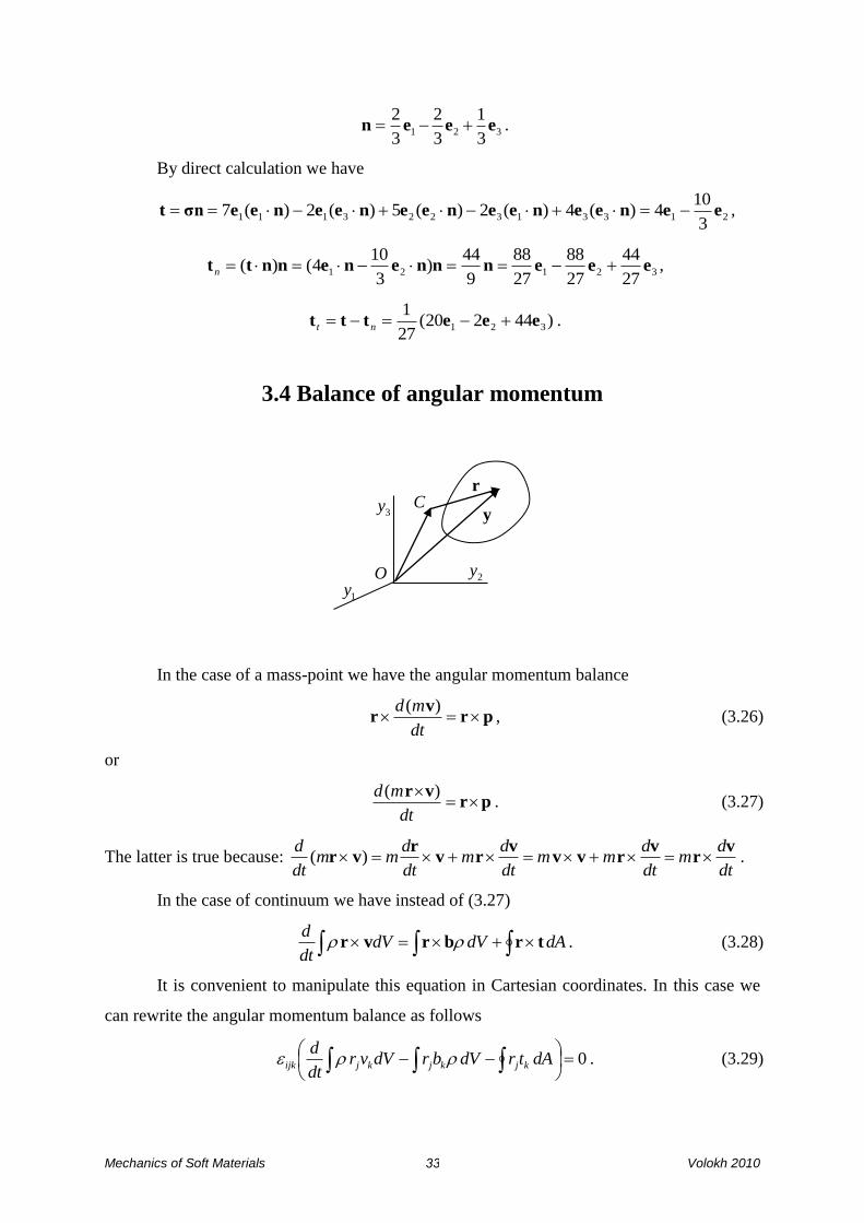
3.4 Balance of angular momentum
In the case of a mass-point we have the angular momentum balance
prv
r dt
md )(, (3.26)
or
prvr
dt
md )(. (3.27)
The latter is true because: dt
dm
dt
dmm
dt
dm
dt
dmm
dt
d vr
vrvv
vrv
rvr )( .
In the case of continuum we have instead of (3.27)
dAdVdVdt
dtrbrvr . (3.28)
It is convenient to manipulate this equation in Cartesian coordinates. In this case we
can rewrite the angular momentum balance as follows
0
dAtrdVbrdVvr
dt
dkjkjkjijk . (3.29)
O
Cr
y3y
2y
1y

Mechanics of Soft Materials Volokh 2010 34
The first and the third terms in the equation above can be calculated by using the
material time derivative of the volume integral and the divergence theorem accordingly
dVy
vvrvv
dt
vdr
dVy
vvr
dt
vrddVvr
dt
d
m
mkjjk
kj
m
mkj
kj
kj
)(
)(
, (3.30)
dVy
r
dVy
r
dVy
r
dAnrdAtr
l
kljkj
l
kljkljl
l
klj
lkljkj
)(
, (3.31)
where we used relation iii OCyr )( with OC fixed.
Substituting (3.30)-(3.31) in (3.29) we get
0])(
[
0
dVvv
yb
y
vv
dt
vdr kjjk
l
klk
m
mk
kjijk
, (3.32)
where the term in the parentheses is the law of the linear momentum balance and it is equal to
zero.
Thus we have
0)( dVdVvv kjijkkjjkijk . (3.33)
The latter equation can be obeyed for the symmetric Cauchy tensor only
T
jkkj σσ , . (3.34)
3.5 Master balance principle
All balance laws enjoy the same structure
dAdVdVdt
dφnξα , (3.35)
where ξ is the volumetric supply of α and φ is the surface flux of α .
Differentiating the integral and using the divergence theorem we localize the balance
law

Mechanics of Soft Materials Volokh 2010 35
ξφvαα
divdivdt
d. (3.36)
The considered balance laws are summarized in the table:
α ξ φ
Mass 0 0
Linear Momentum v b σ
Angular Momentum vr br σr
3.6 Lagrangean description
The description of balance laws was spatial or Eulerian because y was chosen as an
independent variable. In the case of solids (contrary to fluids) it is usually more convenient to
consider x as an independent variable, i.e. it is better to use the referential or Lagrangean
description. The transition from one description to another is simple when the formulas
relating volumes and surfaces before and after deformation are used (see (2.7) and (2.13))
00 det JdVdVdV F , (3.37)
00dAJdA TnFn
. (3.38)
Substituting these equations in the master balance law we get
0000000 dAdVdVdt
dnφξα , (3.39)
where we defined the Lagrangean quantities
)),,((),(0 ttJt xyαxα , (3.40)
)),,((),(0 ttJt xyξxξ , (3.41)
TttJt Fxyφxφ )),,((),(0 . (3.42)
We differentiate (3.39) with respect to time through the integral directly because the
volume does not change and we get the localized balance law in the Lagrangean form
00
0 Div ξφα
t. (3.43)
Here ‘Div’ operator is with respect to the referential coordinates
i
ixe
(...)(...)Div .
Mechanics of Soft Materials Volokh 2010 36
Particularly, the Lagrangean form of the previous table is
0α 0ξ 0φ
Mass 0 0 0
Linear Momentum v0 b0 T
Angular Momentum vr 0 br 0 Tr
where
TttJt FxyσxT )),,((),( (3.44)
is the 1st Piola-Kirchhoff stress tensor (1PK).
The laws of mass, linear and angular momentum balance take the following forms
accordingly
00
t
, (3.45)
i
j
iji bx
T
t
v
t
00
00
)(
Div)(
bT
v
, (3.46)
TTFTTF , (3.47)
Since the 1st Piola-Kirchhoff stress tensor is not symmetric it is convenient to
introduce the 2nd Piola-Kirchhoff stress tensor (2PK)
TJ σFFTFS11 . (3.48)

Mechanics of Soft Materials Volokh 2010 37
4 Isotropic elasticity
4.1 Hyperelasticity
The rheological model for elastic material is a spring. For the classical linear spring,
stress is equal to strain scaled by Young modulus, E ,
E . (4.1)
This equation is called Hooke’s law in honor of Robert Hooke.
Evidently, this constitutive law is a linearization of a more general function describing
a nonlinear spring
)( . (4.2)
Although this function can be fitted in experiments only it is possible to draw some
conclusions about it considering the work of stress on strain
dw )( . (4.3)
In the case of an ideal elastic spring, this work does not depend on the loading history
and it only depends on the initial and final states of the spring – the integration limits in (4.3).
If the integral is path-independent then the integrand should be a full differential
ddw )( . (4.4)
It follows from (4.4) that stress in an ideal elastic spring should be a derivative of the
strain energy with respect to strain
d
dw , (4.5)
where in the case of Hookean elasticity we have: 2/2Ew .
The extension of the simplistic formula (4.5) to 3D is not trivial. Indeed, variety of
stresses and strains can be considered and it is not clear which stress works on which strain.
To clarify that we consider the work of external forces on displacement increments, yu dd ,
over the whole 3D body
0000 dVddAdd byty , (4.6)
E

Mechanics of Soft Materials Volokh 2010 38
where 0t and b0 designate prescribed tractions per the reference area and body forces per
the reference volume, including the inertia forces.
By using the equilibrium equation (3.46) we can rewrite (4.6) in the form
000 )(Div dVddAdd yTyt , (4.7)
where T is the 1st Piola-Kirchhoff stress.
We transform (4.7) as follows
0
0
00
)conditions(boundary 0
00
0000
000
:
)(
)()(
dVd
dVdFT
dVx
ydTdAdynTt
dVx
dyTdV
x
dyTdAdyt
dVdyx
TdAdytd
ijij
j
iijijiji
j
iij
j
iij
ii
i
j
ij
ii
FT
, (4.8)
where the boundary conditions on tractions have been used
00 tTn . (4.9)
Transformation (4.8) means that the incremental work of the external forces is equal
to the incremental work of the internal forces. The work of the internal forces per unit
volume can be designated as follows
FT ddW : . (4.10)
Analogously to 1D case this work is path independent only in the case where
ij
ijF
WT
W
)(,
)( F
F
FT . (4.11)
Here W is called the strain energy and material obeying (4.11) is called hyperelastic.
Evidently, the 1st Piola-Kirchhoff stress makes a work-conjugate couple with the
deformation gradient. It is possible, however, to assume that the strain energy depends on the
Green strain, 2/)( 1FFε T , rather than on the deformation gradient. In this case we have
(prove it!)
im
mjij
mnknkm
mnij
mn
mn
ij FW
F
FFW
F
WT
)(
2
1))(( Fε,
or
Mechanics of Soft Materials Volokh 2010 39
ε
FT
W. (4.12)
On the other hand we have by definition, (3.48),
FST , (4.13)
where S is the 2nd Piola-Kirchhoff stress tensor and, consequently,
ij
ij
WS
W
)(,
)( ε
ε
εS , (4.14)
or
ij
ijC
WS
W
)(2,
)(2
C
C
CS , (4.15)
where 1εFFC 2T is the right Cauchy-Green tensor.
It is possible to show that the considered stress-strain pairs are work-conjugate by the
direct computation (prove it!)
εSFT dd :: . (4.16)
The ‘true’ Cauchy stress is obtained from (4.14)-(4.15) with the help of (3.48) with
FdetJ
TT WJ
WJ F
CFF
εFσ
11 2 . (4.17)
We showed that the strain energy could be defined as a function of various strains. Is
there any preference in the choice of strains? The answer is yes. The strains which are
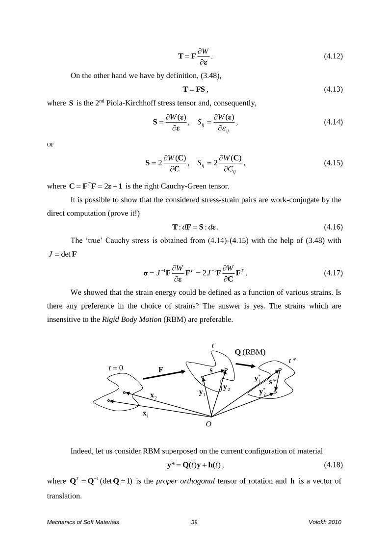
insensitive to the Rigid Body Motion (RBM) are preferable.
Indeed, let us consider RBM superposed on the current configuration of material
)()(* tt hyQy , (4.18)
where )1(det1 QQQ
T is the proper orthogonal tensor of rotation and h is a vector of
translation.
O
0t
t
*t
F
1x
2x
s
*s
)RBM(Q
1y 2y
1y
2y

Mechanics of Soft Materials Volokh 2010 41
This motion preserves the length and the angle. Indeed, we have
QsyyQyys )(*** 1212 , (4.19)
sss1ssQsQssss T*** , (4.20)
cos**
***cos
ps
ps
ps
QpQs
ps
psT
. (4.21)
Thus, a material fiber deforms as follows
xFxQFyQyF
dddd ***
. (4.22)
It is natural to require that the magnitude of the strain energy is not affected by RBM
because there is no straining. The latter means that the function of the strain energy should
obey the following condition
)()( QFF WW . (4.23)
The right Cauchy-Green and Green strain tensor obey this condition automatically
because they are insensitive to RBM
CFFFQQFQFQFFFC1
TTTTT )()(*** , (4.24)
ε1C1Cε 2/)(2/)*(* . (4.25)
4.2 Rivlin’s representation for isotropic material
Ronald Rivlin found (1948) the following representation for the strain energy of
isotropic materials, which is given without proof,
),,()( 321 IIIWW C , (4.26)
CCCC det,2/)}(tr)tr{(,tr 3
22
21 III , (4.27)
that is the strain energy depends on the invariants of the right Cauchy-Green tensor.
Based on this representation we can calculate the stress as follows
CCCCS 3
3
2
2
1
1
22I
I
WI
I
WI
I
WW, (4.28)
where (see (1.47), (1.48), (1.51))
1
33
121 ,,
C
CC1
C1
CI
II
II. (4.29)
Inserting (4.29) in (4.28) we have
Mechanics of Soft Materials Volokh 2010 40
1
3
3
22
1
1
2 CC1SI
WI
I
W
I
WI
I
W. (4.30)
Transition to the Cauchy stress gives us another form of the constitutive law
1BBFSFσ3
3
2
22
1
1
11 2I
WI
I
W
I
WI
I
WJJ T , (4.31)
where
TFFB (4.32)
is the left Cauchy-Green tensor.
We remind that invariants of B coincide with the invariants of C: )()( BC aa II .
4.3 Representation in principal stretches
Sometimes, it is more convenient to formulate the constitutive equations in terms of
principal stretches, i , rather than to use invariants. To make the transition to the principal
stretches we need the spectral representation of the right Cauchy-Green tensor
)3()3(2
3
)2()2(2
2
)1()1(2
1 mmmmmmFFC T , (4.33)
where 2
a and )(am are eigenvalues and eigenvectors of C accordingly.
Since
2
3
2
2
2
13
2
3
2
2
2
3
2
1
2
2
2
12
2
3
2
2
2
11 ,, III , (4.34)
the strain energy can be rewritten as a function of principal stretches 2
ii
),,()( 321 WW C , (4.35)
and we can calculate the energy increment as follows
3
3
2
2
1
1
321 ),,()(
dW
dW
dW
dWdW
C . (4.36)
In order to find 1d we, firstly, get the increment of (4.33)
3
1
)()(2)()(2)()( }2{a
aa
a
aa
a
aa
aa dddd mmmmmmC . (4.37)
Secondly, we pre-multiply it by )1()1(mm as follows
11
)1()1( 2:)( dd Cmm , (4.38)
where we accounted for a
a
1
)()1( mm and 00)( )1()1()1()1( mmmm dd .
Thus, we have from (4.38)

Mechanics of Soft Materials Volokh 2010 42
Cmm dd :)(2
1 )1()1(
1
1
. (4.39)
Repeating this argument for 2d and 3d we get
CC
C dW
dW :)(
, (4.40)
where
3
1
)()(
2
1
a
aa
aa
WWmm
C . (4.41)
Using this derivative we can write the 2nd Piola-Kirchhoff tensor in the form
3
1
)()(12
a
aa
aa
WWmm
CS
. (4.42)
It is remarkable that 2PK stress is coaxial with the right Cauchy-Green tensor because
their principal directions coincide. The latter allows us to directly compute the principal 2PK
stresses
sum) no(1
aa
a
WS
. (4.43)
By using the spectral decomposition of the deformation gradient, (2.35), we can
compute the Cauchy stresses
3
1
)()(
321
1 1
a
aa
a
a
T WJ nnFSFσ
, (4.44)
which is coaxial with the left Cauchy-Green tensor because their principal directions
coincide. The latter allows us to directly compute the principal Cauchy stresses
sum) no(321 a
aa
W
. (4.45)
4.4 Incompressibility
Many soft materials resist volume changes much stronger than the shape changes.
This experimental observation makes it reasonable to assume the material incompressibility
3
0
detdetdetdet1det IJdV
dV T CBFFF . (4.46)
This can be considered as a restriction imposed on deformation
0)(1)( 3 CC I . (4.47)
The incremental form of the restriction can be written as follows

Mechanics of Soft Materials Volokh 2010 43
0:)(
C
CC dd
. (4.48)
Here C / can be interpreted as a stress producing zero work on the strain
increment – the workless stress. Such stress is indefinite since it can always be scaled by an
indefinite parameter, p .
Adding the workless stress to the stress derived from the strain energy we have
TpW
J FCC
Fσ
12 , (4.49)
or, substituting from (4.47) into (4.49),
1FC
Fσ pW T
2 . (4.50)
The unknown multiplier, p , should be obtained from the solution of equilibrium
equations.
In the case of isotropic material we have
2
2211 2)(2 BB1σ WWIWp , (4.51)
where
a
aI
WW
. (4.52)
In terms of the principal stresses and stretches we have instead of (4.45)
sum) no(pW
a
aa
. (4.53)
4.5 Examples of strain energy
In this section we consider some popular strain energy functions, )(CW , which in the
absence of residual stresses should meet the following conditions
01C
1
)(,0)(
WW , (4.54)
or, in the case where the strain energy is a function of principal stretches, ),,( 321 W ,
0)1,1,1(,0)1,1,1(
a
WW
, (4.55)
We start with the Kirchhoff-Saint Venant material
εεεε :)tr(2
)( 2
W , (4.56)

Mechanics of Soft Materials Volokh 2010 44
where and are the Lame constants and the Green strain is 2/)( 1Cε . Differentiating
the strain energy density with respect to the Green strain we obtain 2PK stresses
ijrrij
mnnjmirrkjki
mn
ij
mnrr
ij
kk
ij
mnmn
ij
rrkk
ij
ij
WS
2
2
2
)()(
2
,
ε1εε
S 2)tr(
W. (4.57)
Alternatively, we can rewrite (4.56) and (4.57) in principal stretches
})1()1()1{(4
)3(8
),,( 22
3
22
2
22
1
22
3
2
2
2
1321
W , (4.58)
2/)1(22/)3( 22
3
2
2
2
1 aaS . (4.59)
This classical material model is generally not used for soft materials. In the case of
small strains, (4.57) is the generalized Hooke law. The use of nonlinear strains, however, is
crucial in order to suppress rigid body motions in finite element computations.
Next strain energy function defines the Neo-Hookean incompressible material
1),3()3( 321
2
3
2
2
2
11 JcIcW , (4.60)
where c is a material constant.
The Neo-Hookean model is the simplest one for modeling soft materials. It is often
used as a starting point for the experimental calibration. A popular generalization of (4.60) is
the Yeoh material defined as a polynomial of the first principal invariant, )(1 CI . For example
Hamdi et al (Polymer Testing 25 (2006) 994-1005) calibrated the following Yeoh model for
natural rubber
1,)3()3()3( 3
3
13
2
1211 IIcIcIcW , (4.61)
where
MPa00016.0,MPa014.0,MPa298.0 321 ccc .
Another generalization of the Neo-Hookean model is the Mooney-Rivlin material
which defines the dependence of the strain energy on both the first and second principal
invariants. An example of the incompressible Mooney-Rivlin material was calibrated by
Sasso et al (Polymer Testing 27 (2008) 995-1004)
1,)3()3)(3()3()3()3( 3
2
25214
2
132211 IIcIIcIcIcIcW , (4.62)
Mechanics of Soft Materials Volokh 2010 45
where
MPa00077.0MPa,0076.0MPa,0028.0,MPa039.0,MPa59.0 54321 ccccc .
Further generalization of the previous models is the Ogden material defined as
1,)3(1
321
JWN
p p
p ppp
, (4.63)
where Nppp ,...1,0 .
For example, Hamdi et al (Polymer Testing 25 (2006) 994-1005) calibrated the Ogden
model for styrene-butadiene rubber where 2N and
35.2MPa,025.0,03.3,MPa638.0 2211 .
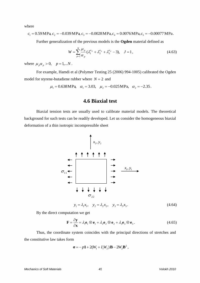
4.6 Biaxial test
Biaxial tension tests are usually used to calibrate material models. The theoretical
background for such tests can be readily developed. Let us consider the homogeneous biaxial
deformation of a thin isotropic incompressible sheet
333222111 ,, xyxyxy . (4.64)
By the direct computation we get
333222111 eeeeeex
yF
. (4.65)
Thus, the coordinate system coincides with the principal directions of stretches and
the constitutive law takes form
2
2211 2)(2 BB1σ WWIWp ,
11
22
22 , yx
11, yx

Mechanics of Soft Materials Volokh 2010 46
4
32
2
321133
4
22
2
221122
4
12
2
121111
2)(2
2)(2
2)(2
WWIWp
WWIWp
WWIWp
. (4.66)
The stresses are homogeneous and the equilibrium equations are satisfied
automatically. From the traction-free boundary conditions on the sheet faces we have
4
32
2
321133 2)(20 WWIWp . (4.67)
Substituting the Lagrange multiplier in the stress tensor we get
)(2)()(2
)(2)()(2
4
3
4
22
2
3
2
221122
4
3
4
12
2
3
2
121111
WWIW
WWIW. (4.68)
Since
2
3
2
2
2
11 tr BI , (4.69)
we can rewrite stresses in the form (prove it!)
))((2
))((2
2
121
2
3
2
222
2
221
2
3
2
111
WW
WW’ (4.70)
where the incompressibility condition enforces
21
3
1
. (4.71)
Equations (4.70) are often used for the experimental calibration of soft materials
under varying ratio of the applied stresses.
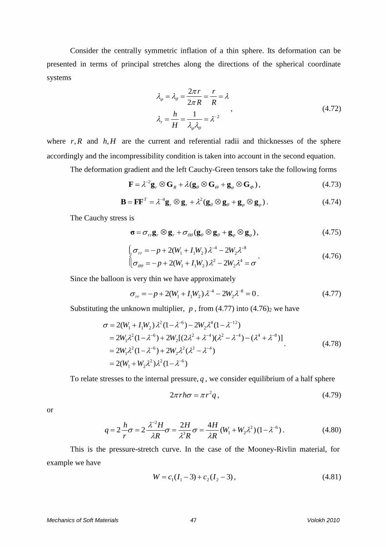
4.7* Balloon inflation
Balloon inflation is another popular deformation used for calibration of soft materials.
r2
hqr
Mechanics of Soft Materials Volokh 2010 47
Consider the centrally symmetric inflation of a thin sphere. Its deformation can be
presented in terms of principal stretches along the directions of the spherical coordinate
systems
21
2
2
H
h
R
r
R
r
r
, (4.72)
where Rr, and Hh, are the current and referential radii and thicknesses of the sphere
accordingly and the incompressibility condition is taken into account in the second equation.
The deformation gradient and the left Cauchy-Green tensors take the following forms
)(2
GgGgGgF
Rr , (4.73)
)(24
ggggggFFB
rr
T . (4.74)
The Cauchy stress is
)( ggggggσ rrrr , (4.75)
4
2
2
211
8
2
4
211
2)(2
2)(2
WWIWp
WWIWprr. (4.76)
Since the balloon is very thin we have approximately
02)(2 8
2
4
211 WWIWprr . (4.77)
Substituting the unknown multiplier, p , from (4.77) into (4.76)2 we have
)1()(2
)(2)1(2
)]())(2[(2)1(2
)1(2)1()(2
622
21
422
2
62
1
844242
2
62
1
124
2
62
211
WW
WW
WW
WWIW
. (4.78)
To relate stresses to the internal pressure, q , we consider equilibrium of a half sphere
qrhr 22 , (4.79)
or
)1()(42
22 62
213
2
WW
R
H
R
H
R
H
r
hq . (4.80)
This is the pressure-stretch curve. In the case of the Mooney-Rivlin material, for
example we have
)3()3( 2211 IcIcW , (4.81)

Mechanics of Soft Materials Volokh 2010 48
2
2
21
1
1 , cI
WWc
I
WW
, (4.82)
and
)1()(4 62
21
ccR
Hq . (4.83)
4.8 Homework
1. Prove (4.12).
2. Prove (4.16).
3. Derive constitutive equations for (4.60).
4. Derive constitutive equations for (4.61).
5. Derive (4.70) from (4.68)-(4.69).
6. Read Section 4.7.
Rr /2.5 5 7.5 10 12.5 15 17.5 20
0
0.2
0.4
0.6
0.8
1
RHc
q
/4 1
12 055.0 cc

Mechanics of Soft Materials Volokh 2010 49
5 Anisotropic elasticity
Rubberlike materials are usually isotropic. It is possible, of course, to strengthen them
by embedding fibers in prescribed directions. Nature does so with the soft biological tissues
which usually consist of an isotropic matrix with the embedded and oriented collagen fibers.
The collagen fibers are aligned with the axis of ligaments and tendons forming one
characteristic direction or they can form two characteristic directions in the case of blood
vessels, heart etc.
5.1 Materials with one characteristic direction
Materials enjoying one characteristic direction are also called materials with
transverse isotropy, i.e. isotropy in the planes perpendicular to the preferred direction. Let us
designate the preferred direction by unit vector 0m in the reference configuration. In this
case the strain energy function ),,,,()( 54321 IIIIIWW C should additionally depend on two
more invariants
)(: 0000004 mmCmFFmFmFmmm
Cmm
TI , (5.1)
)(: 00
2
5 mmC I , (5.2)
where
0Fmm (5.3)
is not a unit vector.
The fourth invariant, 4I , has a clear physical meaning of the squared stretch in the
characteristic direction. The dyad in the parentheses is often called the structural tensor,
which characterizes the internal design of material.
Differentiating (5.1) and (5.2) with respect to C we get accordingly
00
4 mmC
I, (5.4)
00005 mCmCmm
C
I, (5.5)
Accounting for (4.29) and (5.4)-(5.5) we calculate the constitutive equation

Mechanics of Soft Materials Volokh 2010 51
)}(){(2
22
00005004
1
332211
5
1
mCmCmmmmCC1
CCS
WWWIWWIW
I
I
WW
a
a
W
a
a
,(5.6)
or
)}(){(2 5433
2
2211
1
1
mBmBmmmm1BB
FSFσ
WWWIWWIWJ
J T
, (5.7)
where TFFB is the left Cauchy-Green tensor.
In the case of incompressible material we have instead of (5.7)
)}(){(2 54
2
2211 mBmBmmmmBB1σ WWWWIWp . (5.8)
5.2 Materials with two characteristic directions
In the case of two preferred directions we designate the second characteristic unit
vector with prime 0m in the reference configuration the strain energy function
),,,,,,,()( 87654321 IIIIIIIIWW C should additionally depend on three more independent
invariants
)(: 006 mmC I , (5.9)
)(: 00
2
7 mmC I , (5.10)
)(: 008 mmC I , (5.11)
where
0mFm (5.12)
is not a unit vector.
Invariants 76 , II are analogous to 54 , II while invariant 8I is related to both
characteristic directions.
Differentiating (5.9) - (5.11) with respect to C we get accordingly
006 mm
C
I, (5.13)
00007 mmCmCm
C
I, (5.14)
)(2
10000
8 mmmmC
I. (5.15)
We notice that the last derivative preserves symmetry.

Mechanics of Soft Materials Volokh 2010 50
Now the Cauchy stress takes form
)(
)(22
)(22
22)(2
8
76
54
33
2
2211
mmmm
mmBmBmmm
mBmBmmmm
1BBσ
W
WW
WW
WIWWIWJ
. (5.16)
In the case of incompressible material we have instead of (5.16)
)(
)(22
)(22
2)(2
8
76
54
2
2211
mmmm
mmBmBmmm
mBmBmmmm
BB1σ
W
WW
WW
WWIWp
. (5.17)
5.3 Fung model of biological tissue
The presented way of introducing characteristic directions is not unique for a
description of anisotropy. The classical works of Y.C. Fung and his disciples introduced
anisotropy by using the Green strain 2/)( 1Cε as follows
...):::exp()::(::2
1)( 0 εκεεγεβεεαεε W ,
or
...)exp()(2
10 klijijklijijpqmnmnpqklijijklW . (5.18)
Here κγβα ,,,, 0 are scalars, second- and fourth- order tensors of material constants which
should be defined in experiments.
The exponential function allows modeling stiffening typical of soft biological tissues.
As an example of the calibrated Fung strain energy we present the constitutive model of a
rabbit carotid artery
}1)222{exp(2
654
2
3
2
2
2
1 ZZRRZZRRZZRR ccccccc
W , (5.19)
with KPa95.26c the dimensional and ic s are dimensionless: 0089.01 c , 9925.02 c ,
4180.03 c , 0193.04 c , 0749.05 c , 0295.06 c .
5.4 Artery under blood pressure
We consider inflation of an artery under blood pressure. The corresponding Boundary
Value Problem (BVP) includes equations of momentum balance (equilibrium)
Mechanics of Soft Materials Volokh 2010 52
0σ div , (5.20)
constitutive law
TWp F
εF1σ
, (5.21)
and boundary conditions on placements and tractions
tσnyy or , (5.22)
where 'div' operator is with respect to the current coordinates y ; σ is the Cauchy stress
tensor; 1 is the second order identity tensor; p is an unknown multiplier of the workless
stress; 2/)( 1FFε T is the Green strain tensor; W is the strain energy; t is traction per
unit area of the current surface with the unit outward normal n ; and the barred quantities are
prescribed.
We consider the radial inflation of an artery as a symmetric deformation of an infinite
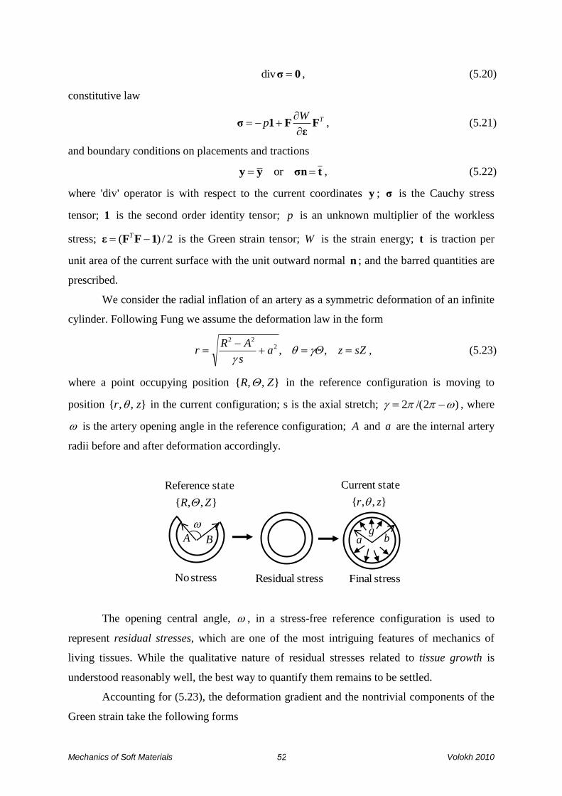
cylinder. Following Fung we assume the deformation law in the form
sZzas
ARr
,,2
22
, (5.23)
where a point occupying position },,{ ZR in the reference configuration is moving to
position },,{ zr in the current configuration; s is the axial stretch; )2/(2 , where
is the artery opening angle in the reference configuration; A and a are the internal artery
radii before and after deformation accordingly.
The opening central angle, , in a stress-free reference configuration is used to
represent residual stresses, which are one of the most intriguing features of mechanics of
living tissues. While the qualitative nature of residual stresses related to tissue growth is
understood reasonably well, the best way to quantify them remains to be settled.
Accounting for (5.23), the deformation gradient and the nontrivial components of the
Green strain take the following forms
A B
},,{
state Reference
ZR
stress No stress Residual stress Final
},,{
stateCurrent
zr
a bg

Mechanics of Soft Materials Volokh 2010 53
ZzRr sR
r
rs
RGgGgGgF
, (5.24)
2/}1{
2/}1)/{(
2/}1)/{(
2
2
2
s
Rr
rsR
ZZ
RR
, (5.25)
where ZR GGG ,, and zr ggg ,, are the orthonormal bases in cylindrical coordinates at
the reference and current configurations accordingly.
Accounting for (5.21), (5.23)-(5.25) and assuming that the stored energy depends on
the nontrivial strain components only we get the following nonzero components of the
Cauchy stress
ZZ
zz
RR
rr
Wsp
W
R
rp
W
sr
Rp
2
2
2
2
2
)(
)(
. (5.26)
Besides, there is only one nontrivial equilibrium equation
0
rr
rrrr . (5.27)
The traction boundary conditions are
0)(
)(
br
gar
rr
rr
, (5.28)
where ba, are the inner and outer radii of the artery after the deformation, which were equal
to BA, before the deformation accordingly; and g is the internal pressure.
We integrate equilibrium equation (5.27) over the wall thickness with account of
boundary conditions (5.28) and we get
)(
2
2
2
2)()(
)()()(
ab
a RR
ab
a
rrr
drW
R
rW
rs
R
r
drag
, (5.29)
where )/()()( 222 sABaab .
Equation (5.29) presents the pressure-radius (g-a) relationship, which we examine
below. Before doing that, however, we introduce dimensionless variables as follows
A
bb
A
aa
A
RR
A
rr
c
WW
c
gg ;;;; , (5.30)
Mechanics of Soft Materials Volokh 2010 54
where c is the shear modulus.
Substituting (5.30) in (5.29) we get
)(
2
2
2
2 )(
)()(
ab
a RR r
rdW
R
rW
rs
Rag
, (5.31)
where
)/()1)/(()( 22 sABaab , (5.32)
1)( 222 arsR . (5.33)
The dimensionless multiplier cpp / is obtained from (5.27) and (5.28)1 by
integration
r
a RRRR
dW
R
W
s
Ragr
W
rs
rRrp
)()(
)()(
)(
)()()(
)(
)()(
2
2
2
2
2
2
, (5.34)
and normalized stresses take the form
ZZ
zzzz
RR
rrrr
Wsp
c
W
R
rp
c
W
rs
Rp
c
2
2
2
2
2
)(
)(
. (5.35)
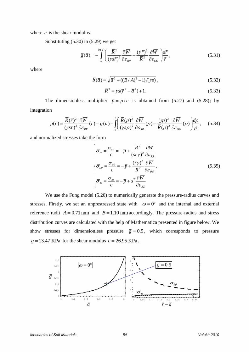
We use the Fung model (5.20) to numerically generate the pressure-radius curves and
stresses. Firstly, we set an unprestressed state with 0 and the internal and external
reference radii mm71.0A and mm10.1B accordingly. The pressure-radius and stress
distribution curves are calculated with the help of Mathematica presented in figure below. We
show stresses for dimensionless pressure 5.0g , which corresponds to pressure
KPa47.13g for the shear modulus KPa95.26c .
0 0.05 0.1 0.15 0.2 0.25 0.3 0.35
2
4
6
8
1 1.2 1.4 1.6 1.8 2
0
0.25
0.5
0.75
1
1.25
1.5
g
a
zzrr
5.0g
ar
0
Mechanics of Soft Materials Volokh 2010 55
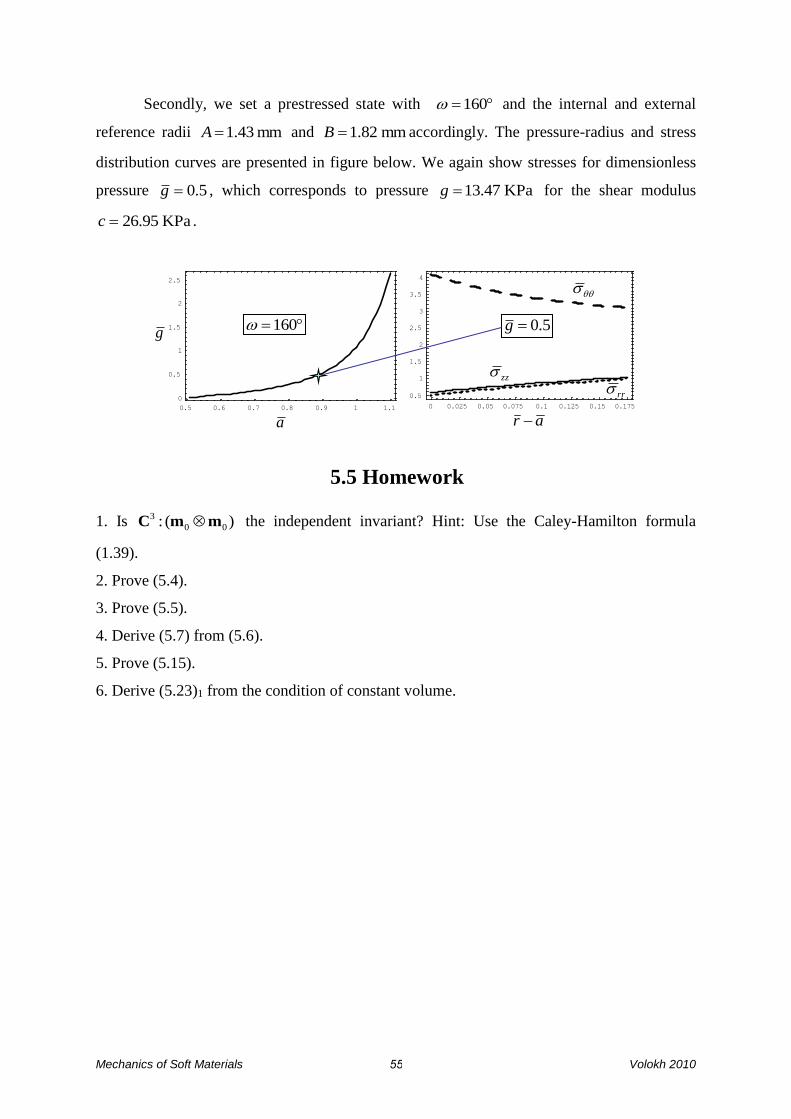
Secondly, we set a prestressed state with 160 and the internal and external
reference radii mm43.1A and mm82.1B accordingly. The pressure-radius and stress
distribution curves are presented in figure below. We again show stresses for dimensionless
pressure 5.0g , which corresponds to pressure KPa47.13g for the shear modulus
KPa95.26c .
5.5 Homework
1. Is )(: 00
3mmC the independent invariant? Hint: Use the Caley-Hamilton formula
(1.39).
2. Prove (5.4).
3. Prove (5.5).
4. Derive (5.7) from (5.6).
5. Prove (5.15).
6. Derive (5.23)1 from the condition of constant volume.
0 0.025 0.05 0.075 0.1 0.125 0.15 0.175
0.5
1
1.5
2
2.5
3
3.5
4
0.5 0.6 0.7 0.8 0.9 1 1.1
0
0.5
1
1.5
2
2.5
g
a
zz
rr
5.0g
ar
160

Mechanics of Soft Materials Volokh 2010 56
6 Viscoelasticity
Rubberlike materials and soft biological tissues can exhibit a time-delayed response.
For example, stresses can decrease under the constant strains – stress relaxation – or strains
can increase under the constant stresses – creep. Such phenomena are usually related to
viscosity, which is a fluid-like property of solids.
6.1 Rheological model
To describe viscosity we start with a simple one-dimensional model, also called
rheological. Rheological models are prototypes for general three-dimensional constitutitive
theories. For example, the spring model is a prototype for hyperelasticity theories. To account
for viscoelasticity we will use the device shown in the figure below.
This rheological model represents the so-called ‘standard solid’, which includes the
classical elasticity due to the top linear spring with the Young modulus E and viscosity due
to the chain of the linear spring with Young modulus E and the linear dashpot with the
viscosity coefficient . The dashpot provides the time delay in the mechanical response of
the device.
We assume, for the sake of simplicity, that the device has a unit length and a unit area
and, consequently, strains and stresses are equal to elongations and forces. The resulting
stress is composed of stresses acting on the top and bottom elements of the device
qE
, (6.1)
where E is the stress in the top spring; is the strain of the whole device; and q is
the ‘viscous’ stress in the bottom element.
The viscous stress can be calculated considering the dashpot with the linear
proportionality between the stress and strain rate in as in the case of Newtonian fluids
E
q
E
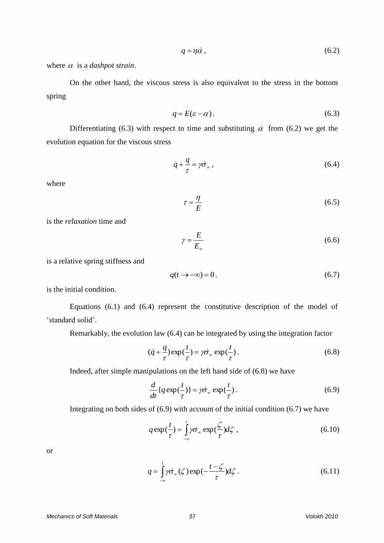
Mechanics of Soft Materials Volokh 2010 57
q , (6.2)
where is a dashpot strain.
On the other hand, the viscous stress is also equivalent to the stress in the bottom
spring
)( Eq . (6.3)
Differentiating (6.3) with respect to time and substituting from (6.2) we get the
evolution equation for the viscous stress
q
q , (6.4)
where
E
(6.5)
is the relaxation time and
E
E (6.6)
is a relative spring stiffness and
0)( tq . (6.7)
is the initial condition.
Equations (6.1) and (6.4) represent the constitutive description of the model of
‘standard solid’.
Remarkably, the evolution law (6.4) can be integrated by using the integration factor
)exp()exp()(
ttqq . (6.8)
Indeed, after simple manipulations on the left hand side of (6.8) we have
)exp()}exp({
ttq
dt
d . (6.9)
Integrating on both sides of (6.9) with account of the initial condition (6.7) we have
d
tq
t
)exp()exp( , (6.10)
or
d
tq
t
)exp()( . (6.11)
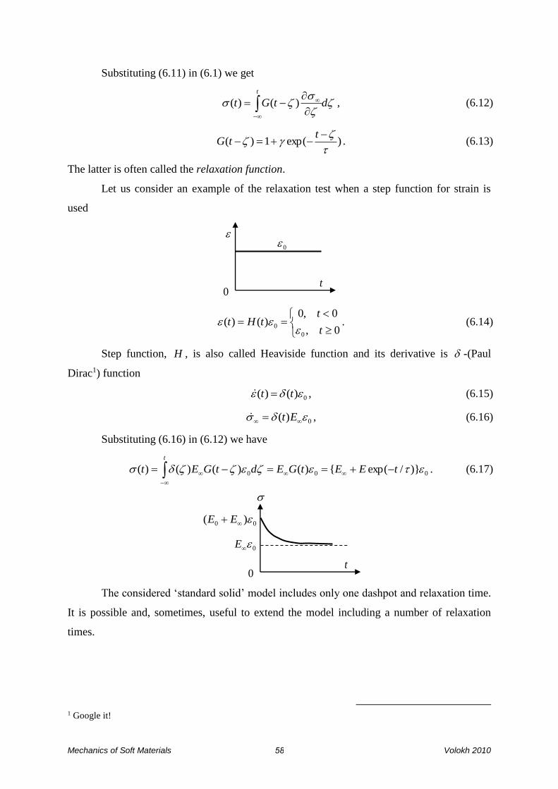
Mechanics of Soft Materials Volokh 2010 58
Substituting (6.11) in (6.1) we get
dtGt
t
)()( , (6.12)
)exp(1)(
ttG . (6.13)
The latter is often called the relaxation function.
Let us consider an example of the relaxation test when a step function for strain is
used
0,
0,0)()(
0
0t
ttHt
. (6.14)
Step function, H , is also called Heaviside function and its derivative is -(Paul
Dirac1) function
0)()( tt , (6.15)
0)( Et , (6.16)
Substituting (6.16) in (6.12) we have
000 )}/exp({)()()()( tEEtGEdtGEt
t
. (6.17)
The considered ‘standard solid’ model includes only one dashpot and relaxation time.
It is possible and, sometimes, useful to extend the model including a number of relaxation
times.
1 Google it!
0
0t
0t
0E
00 )( EE

Mechanics of Soft Materials Volokh 2010 59
In this case, constitutive equations take the following form accordingly
i
iq , (6.18)
i
i
ii
qq , (6.19)
where
i
ii
ii
EE
E
, , (6.20)
0)( tqi . (6.21)
The relaxation function (6.13) takes form
i i
i
ttG )exp(1)(
, (6.22)
6.2 Constitutive equations
The rheological model developed in the previous paragraph can serve as a prototype
for the constitutive equations of solids. Particularly, we can define the following constitutive
equations in 3D by analogy with (6.18), (6.19), and (6.21)
i
iQSS , (6.23)
SQ
Q
i
ii
, (6.24)
0Q )(ti . (6.25)
where S is the second Piola-Kirchhoff stress tensor; iQ is the ith internal stress-like variable.
Evolution equation (6.24) can be integrated analytically as in the previous section and
we get the convolution integral
E
11E
22E
Mechanics of Soft Materials Volokh 2010 61
dtGt
t
SS )()( , (6.26)
i i
ttG )exp(1)(
, (6.27)
where the elastic stress is derived from the strain energy, W ,
C
S
W2 . (6.28)
Unfortunately, the direct use of the described model is not practical because most
materials exhibit different responses concerning the volume and shape changes. To make the
difference Flory (1961) proposed the volumetric-deviatoric split of the deformation gradient
FF3/1J , (6.29)
where
FF3/1 J (6.30)
is the isochoric or distortional part of deformation that preserves volume
1det F . (6.31)
Accordingly, tensor 13/1J presents the dilatational, i.e. volume-changing, part of the
deformation.
Barring the distortional quantities we have for the Cauchy-Green tensor
CFFFFC3/23/2 JJ TT . (6.32)
Now the strain energy can be considered as a function of the dilatational and
distortional deformations and the constitutive equation (6.28) takes form
isovol
:22),(
2
SS
C
C
CCC
CS
WJ
J
WJW. (6.33)
The first and the second terms on the right-hand side of (6.33) designate the
volumetric and isochoric parts of the stress. We calculate them as follows.
1
2
1det
C
C
C
CJ
J, (6.34)
13/23/2
3
1
C
CJ
J, (6.35)
*3
1)( 3/213/23/2
1CCC
C
C
C
JJ
J, (6.36)
where *1 is the fourth-order unity tensor with components

Mechanics of Soft Materials Volokh 2010 60
jmik
km
ij
ijkmC
C
*)(1 . (6.37)
Thus, the volumetric and isochoric responses can be presented using (6.33), (6.34),
and (6.36) as follows
1vol
CS J
J
W, (6.38)
)2Dev(2:)3
1*( 3/2
Dev
13/2iso
CCCC1S
WJ
WJ
, (6.39)
where we introduced the Lagrangean deviator operator ‘Dev’.
By using the Flory split, we can finally reformulate the constitutive equations of
voscoelasticity in the following differential form
i
iQSSSisovol , (6.40)
iso
SQ
Q
i
ii
, (6.41)
0Q )(ti . (6.42)
Integrating (6.41)-(6.42), we get
d
tt
i
i
iso
)exp(S
Q . (6.43)
It is clear now that only distortional deformations are rate-sensitive.
6.3 Numerical integration of constitutive equations
Constitutive equations (6.40), (6.43) are of integral type and it is important to develop
a numerical procedure for calculating stresses for the given strain – the stress update
procedure. As the first step in the direction of the integration algorithm, we assume that
deformation starts only at time 0t and all stress variables are zero prior to this time. The
latter assumption allows us to rewrite (6.43) in the form
d
tt
i
i
0
iso
)exp(S
Q . (6.44)
Let us now partition the time interval of interest into small increments
nn ttt 1 , (6.45)
where subscripts designate the point on the time scale.
Mechanics of Soft Materials Volokh 2010 62
We assume that the deformation state of the body is fully determined at time nt
x
u1
x
yF
nn
n , (6.46)
nnnn
T
nnnn JJ CCFFCF3/2,,det , (6.47)
where ),( nn txyy .
We also assume that all stresses are known at time nt : ninn QSS ;; isovol
.
Solution of the balance equations at time ttt nn 1 allows us to find kinematical
quantities
x
u1
x
yF
11
1nn
n , (6.48)
1
3/2
1111111 ,,det
nnnn
T
nnnn JJ CCFFCF , (6.49)
and, subsequently, stresses
1
1
1
vol
1
n
n
n JJ
WCS , (6.50)
)2(Dev1
1n
3/2
1
iso
1
n
nn
WJ
CS . (6.51)
It remains to update the internal variables (6.44) only.
Various computational schemes can be used for updating 1niQ . We proceed by
writing (6.44) in the form
d
td
t n
n
n t
t i
n
t
i
nni
1 iso
1
0
iso
11 )exp()exp(
SSQ . (6.52)
The first term on the right-hand side of (6.52) is calculated as follows
)exp()exp()exp()exp(0
iso
0
iso
i
ni
t
i
n
i
t
i
n td
ttd
tt
ni
nn
QSS
Q
.(6.53)
To integrate the second term on the right-hand side of (6.52) we make the following
approximation for the exponent
)2
exp()exp(
2/
1
ii
tttt
n tt
nn
, (6.54)
and, consequently,
Mechanics of Soft Materials Volokh 2010 63
))(2
exp()exp( isoiso
1
iso
1
1
nn
i
t
t i
n td
tn
n
SSS
. (6.55)
Substituting (6.53) and (6.55) in (6.52) we have finally
)2
exp()()exp( isoiso
11
i
nn
i
nini
tt
SSQQ . (6.56)
6.4 Homework
1. Prove (6.34).
2. Prove (6.35).
3. Prove (6.36).
4. Derive (6.39) from (6.33)-(6.36).

Mechanics of Soft Materials Volokh 2010 64
7 Chemo-mechanical coupling
Previously, we attributed displacements, stresses, strains to a material point or an
infinitesimal material volume. In many cases of practical interest additional parameters
reflecting the presence of the specific material/chemical constituents are required. For
example, gels composed of a network of cross-linked molecules swell when a solvent
migrates through it. The concentration of the solvent is changing and the gel deforms
(remember diapers!). When dried the gel shrinks analogously to the consolidation process in
soils where the applied load enforces water to leave the solid skeleton. Soft biological tissues
like cartilage exhibit sound alterations of the fluid phase during walking. Hard materials like
metals and ceramics can undergo the internal atomic migrations. For example, some hard
materials can absorb and store large amounts of hydrogen. In many cases, not only the
concentration of the constituents change but the process of their diffusion is important. We
will always assume that the diffusion process is slow enough to ignore the inertia effects.
7.1 Governing equations
Governing equations accounting for the chemo-mechanical coupling should include
the equations of balance and boundary conditions for the chemical/material constituents of
interest and, besides, the constitutive law. We consider only one additional chemical/material
component of interest for the sake of simplicity. Generalization for the case of a few
components is trivial. The results of Sections 3.5 and 3.6 on Eulerian and Lagrangean forms
of the master balance equations are crucial.
The integral form of the Eulerian balance law is
dAdVdVcdt
dnφ , (7.1)
where c is the true concentration, i.e. the number of molecules (or moles) of the constituent
per unit current volume; is its volumetric supply; and φ is its flux through the current
body surface with the unit outward normal n .
Localizing this equation by getting rid of the integrals, we formulate the field balance
equation
φv div)(div c
t
c, (7.2)

Mechanics of Soft Materials Volokh 2010 65
where iiy e /(...)(...)div is calculated with respect to spatial coordinates, and boundary
conditions
0)(or cfnnφ , (7.3)
where the barred quantity is prescribed and f is a boundary constraint imposed on the
concentration.
The initial condition takes form
ctc )0( . (7.4)
Since the deformed boundary is generally not known in advance, it can be
advantageous to use the Lagrangean or referential description where the equations (7.1)-(7.4)
take the following forms accordingly
0000000 dAdVdVcdt
dnφ , (7.5)
000 Div
φ
t
c, (7.6)
0)(or 00000 cfnnφ , (7.7)
00 )0( ctc . (7.8)
where iix e /(...)(...)Div is calculated with respect to referential coordinates.
The Eulerian and Lagrangean quantities are related as follows (see Part 3 Balance
Laws)
00 det JdVdVdVJ
F , (7. 9)
00dAJdA TnFn
, (7.10)
0
1cJc , (7.11)
0
1 J , (7.12)
0
1Fφφ
J . (7.13)
In addition to the balance laws, we have to formulate the constitutive equations that
can generally be written in the following form
)/,,( 0000 xCφφ cc , (7.14)
)/,,( 0000 xC cc , (7.15)
where FFCT is the right Cauchy-Green deformation tensor.

Mechanics of Soft Materials Volokh 2010 66
It is important to emphasize that the flux should depend on the gradient of the
concentration, x /0c , to provide the second order of the balance equations. It should also
be noticed that constitutive relations (7.14)-(7.15) were formulated for the Lagrangean
quantities while it could alternatively be done for the Eulerian quantities.
7.2 Diffusion through polymer membrane
Based on the described theoretical framework we examine the problem of diffusion of
a liquid through the polymer membrane that was considered in experiments of Paul and Ebra-
Lima (J. Appl. Polymer Sci. 14 (1970) 2201-2224).
A thin polymer layer is placed on a permeable porous plate and the liquid diffuses
through the membrane under pressure 12 pp . We assume that the body force and source are
zero: 0b 0 and 00 ; and the process is steady state: 00 c . Under these assumptions the
balance equations reduce to
0Div 0 φ , (7.16)
0T Div . (7.17)
The constitutive equations can be defined as follows, for example,
C
CFT
),(2 0cW
, (7.18)
x
CMφ
),( 00 c , (7.19)
0
0 ),(
c
cW
C , (7.20)
Polymer
Porous plate
Liquid
l11, yx
33 , yx
2p
1p
Mechanics of Soft Materials Volokh 2010 67
where M is the mobility tensor; and is the chemical potential.
Motivated by many practical situations it is reasonable to assume that the ground
material (polymer) in the reference state is incompressible and the volume of the material is
altering only due to the supply of new species (molecules of the liquid). This assumption can
be formalized by using the following constraint
01),( 00 Jvcc F , (7.21)
where v is the volume of one molecule of the liquid.
The increment of this constraint takes form
0:: 00
0
FFFF
TJcvcc
. (7.22)
Multipliers v and TJ F in (7.22) represent the workless chemical potential and
stress accordingly, which can be scaled by arbitrary factor . With account of (7.22) we
modify (7.18) and (7.20) as follows
TT JJW
FTF
CFT
T
~
2
~
, (7.23)
vc
W
0
. (7.24)
Since the thickness of the membrane is small as compared to the characteristic lengths
of the device, we can consider the field variations in the lateral directions only. Specifically,
we set the deformation and concentration gradients in the following forms accordingly
3332211 )( eeeeeeF x , (7.25)
3030 eφ . (7.26)
Substituting (7.25)-(7.26) in (7.23) and (7.19), we get the following non-trivial
stresses and fluxes
112211
~TTT , (7.27)
3333
~TT , (7.28)
3
3303x
M
. (7.29)
We notice that the traction/placement boundary conditions take the following forms
on the upper and lower surfaces of the membrane accordingly
233 )( pLT , (7.30)

Mechanics of Soft Materials Volokh 2010 68
0)0(3 y . (7.31)
Since the stress tensor is divergence-free and constant33 T , we can obtain the
unknown multiplier from boundary condition (7.30)
233
~pT . (7.32)
Substituting (7.32) in (7.24) we get for the chemical potential
233
0
~vpTv
c
W
. (7.33)
We also notice that due to the molecular incompressibility condition the concentration
is related to the stretch as follows
10 vc . (7.34)
Substituting (7.33)-(7.34) and (7.29) in (7.16) we get a second order ordinary
differential equation of the chemical balance in term of stretches. To solve it we need to
impose two boundary conditions
0)()( 111 vpf , (7.35)
0)()( 222 vpf , (7.36)
where )0(1 and )(2 L .
We define the mobility tensor and the Helmholtz free energy function as follows
101
0 )( CMkT
Dcvc , (7.37)
mixing ofEnergy
00
0
energy Elastic
321
2
3
2
2
2
1 )1
]1
1log[(])log[23(2
1
vcvcvc
v
kTNkTW
, (7.38)
where and are dimensionless material constants; D is the diffusion coefficient for the
solvent molecules; k is the Boltzmann constant; T is the absolute temperature; N is the
number of polymer chains in the gel divided by the reference volume; is a dimensionless
parameter; and i are the principal stretches.
Substituting (7.37) in (7.26) and accounting for (7.25) we get
3
201
003 )(xkT
Dcvc
. (7.39)
Differentiating (7.38) with respect to stretches and concentration and accounting for
(7.34) we find
)(~ 1
33
NkTT , (7.40)

Mechanics of Soft Materials Volokh 2010 69
)11
(log2
0
kT
c
W. (7.41)
Substituting (7.40)-(7.41) in (7.33) we have finally
2
1
2)()
11(log vpNvkTkT
. (7.42)
Substituting (7.42) in (7.29) and (7.16), we have the second-order ordinary
differential equation, which is completed by boundary conditions (7.35)-(7.36).
Based on the numerical solution of the boundary-value problem it is possible to
calculate the increase of the flux through the membrane with the increase of the pressure –
see the figure below for the toluene-rubber data shown in the table. Remarkably, the flux
increase is not proportional to the pressure increase. The latter is a well-established
experimental fact.
k Nm/K1038.1 23
T K033
1p 25 N/m10
v 329 m107.17
D /sm1036.2 210
N 325 m/11036.6
L m1065.2 4
425.0
7.5
3
0 100 200 300 400
0
2
4
6
8
10
03vTheory
Experiment
]psi[12 pp
]daycm
cm[
2
3

Mechanics of Soft Materials Volokh 2010 71
7.3 Homework
1. Derive (7.40) and (7.41) from (7.38) and (7.34).
2. Read Hong et al (J. Mech. Phys. Solids 56 (2008) 1779-1793).
3. Write a half-page explanation of the physical meaning of the chemical potential based on a
literature review and Google search.

Mechanics of Soft Materials Volokh 2010 70
8 Electro-mechanical coupling
Soft polymer materials are dielectric, i.e. they do not conduct the electric current.
However, electroactive polymers can deform in response to electric fields. This property is
increasingly used in actuators or artificial muscles that have a great potential of practical
applications. We will consider the basic electro-elasticity of soft materials at large strains.
8.1 Electrostatics
Electron presents the smallest negative charge of (Coulomb) C106.1 19e . All
other charges, both positive and negative, are multipliers of the electron charge. The
charges can be free leading to the electric current or bound as in the case of electroactive
dielectrics. Since the number of charges in the material volumes that we consider is large, we
will always mean the continuum average in the subsequent considerations.
Charges create electric fields that produce forces on other charges. For example, the
force on charge Q is2
Ef Q , (8.1)
where E is the electric field.
According to the experimentally validated Coulomb’s law the force between charges
Q and Q placed at points y and y accordingly is inversely proportional to the squared
distance between the charges
)(
3
04
yE
yy
yyf
QQ , (8.2)
where er)(Farad/met F/m10854.8 12
0
is called the permittivity of space.
Based on (8.2) we can write the electric field by superposing many charges smeared
over the space with the charge density q
Vdq
3
0
)(4
1)(
yy
yyyyE
. (8.3)
Based on (8.3) we can obtain (without proof) the Gauss law for a space volume, V ,
enclosed with a surface, A , with the outward unit normal n
qdVdAnE0 . (8.4)
2 See also Jackson JD (1999) Classical Electrodynamics. John Wiley & Sons.
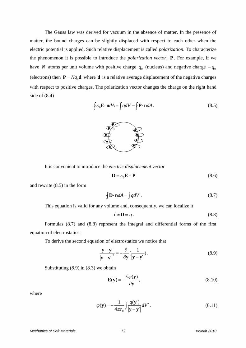
Mechanics of Soft Materials Volokh 2010 72
The Gauss law was derived for vacuum in the absence of matter. In the presence of
matter, the bound charges can be slightly displaced with respect to each other when the
electric potential is applied. Such relative displacement is called polarization. To characterize
the phenomenon it is possible to introduce the polarization vector, P . For example, if we
have N atoms per unit volume with positive charge 0q (nucleus) and negative charge 0q
(electrons) then dP 0Nq where d is a relative average displacement of the negative charges
with respect to positive charges. The polarization vector changes the charge on the right hand
side of (8.4)
dAqdVdA nPnE0 . (8.5)
It is convenient to introduce the electric displacement vector
PED 0 (8.6)
and rewrite (8.5) in the form
qdVdAnD . (8.7)
This equation is valid for any volume and, consequently, we can localize it
qDdiv . (8.8)
Formulas (8.7) and (8.8) represent the integral and differential forms of the first
equation of electrostatics.
To derive the second equation of electrostatics we notice that
)1
(3
yyyyy
yy
. (8.9)
Substituting (8.9) in (8.3) we obtain
y
yyE
)()(
, (8.10)
where
Vd
q
yy
yy
)(
4
1)(
0 . (8.11)

Mechanics of Soft Materials Volokh 2010 73
is called the electric potential or voltage.
To clarify the physical meaning of the electric potential we consider the work that
should be done against the electric field in order to move charge Q from point 1y to point 2y
)()( 12
2
1
2
1
yyyy
yE
y
y
y
y
QQdQdQW
. (8.12)
Thus, the work is equal to the difference in the electrical potentials at points 1y and
2y times charge Q .
Since the integral in (8.12) does not depend on the integration path we have for any
closed curve l
0 yE d . (8.13)
By building any surface A on the curve l and using the Stokes formula we can
rewrite (8.13) in the form
0)(curl dAd nEyE . (8.14)
Since the surface can be chosen arbitrarily, we can localize the integral equation as
follows
0E curl . (8.15)
We notice that the electric field derived from the electric potential always obeys
(8.16): see (1.96).
Formulas (8.14) and (8.15) represent the integral and differential forms of the second
equation of electrostatics.
With the help of (8.7) and (8.13) we can derive the boundary conditions on a surface
separating two materials with different electric fields and displacements.
n
A
l

Mechanics of Soft Materials Volokh 2010 74
Firstly, we consider a small cylinder with the base area A and height 0h . In this
case, the left- and right- hand sides of (8.7) take the following forms accordingly
AAAdA nDDnDnDnD )()( 1212 , (8.16)
AqqdV A , (8.17)
where Aq is a charge on the boundary surface.
Substituting (8.16) and (8.17) in (8.7) we can write the following boundary condition
Aq nDD )( 12 . (8.18)
Secondly, we consider a closed path, l , whose long arm directions are defined by the
cross product of the surface tangent, s , and normal, n , vectors. In this case, (8.13) takes the
following form
0)(
)()(
21
21
nEnEs
snEsnEyE
l
lld
. (8.19)
Since (8.19) is correct for any tangent s we obtain the second boundary condition
0nEE )( 21 . (8.20)
Finally, we notice that the polarization vector should be defined as a function of the
electric field or, in other words, the constitutive equation should be written in the form
)(EPP . (8.21)
The simplest form of the constitutive equation in the case of isotropic media is the
proportionality between the polarization and the electric field
EP 0 , (8.22)
where is called the electric susceptibility of the medium.
Substituting (8.22) in (8.6) we get
EED
)1(0 , (8.23)
n
0h
11,DE
22 ,DE
Aq
Boundary surface
A
l
s l

Mechanics of Soft Materials Volokh 2010 75
where is called the electric permittivity and the ratio 1/ 0 is called the dielectric
constant.
8.2 Angular momentum balance
Equations of the angular momentum balance (3.28) should be modified to include the
body couple due to the electric field, K ,
dAdVdVdt
dtrKbrvr )( . (8.24)
Localizing this equation as it was done in Section 3.4 we obtain
0 ikjijk K . (8.25)
This equation means that the Cauchy stress is not symmetric anymore in the presence of the
electric field: Tσσ !
Though there are a number of theories defining the constitutive equation for the
electric body force and body couple (Pao YH (1978) Electromagnetic Forces in Deformable
Continua. In: Mechanics Today, vol.4, ed. S. Nemat-Nasser. Pergamon Press.), all of them
reduce to the same form in the case of electrostatics and zero distributed body charge, 0q ,
PEb )grad( , (8.26)
EPK . (8.27)
Following Maxwell’s idea for magnetism, some authors represent the electric body
force as a divergence of the “Maxwell stress” tensor, Mσ ,
MσPEb div)grad( . (8.28)
Such representation is not unique and it can take the following popular form, for example,
1EEPEEσ
D
)(2
)( 00
M . (8.29)
Combining the elastic and Maxwell stresses it is possible to introduce the total stress
Mσσσ ~ , (8.30)
which obeys the equilibrium equation (3.25) without body forces
0σ ~div . (8.31)
Substituting from (8.27), (8.29), and (8.30) in the equation (8.25) of the angular
momentum balance we get
0~ kjijk , (8.32)

Mechanics of Soft Materials Volokh 2010 76
i.e. the total stress is symmetric, contrary to the Cauchy stress
Tσσ ~~ . (8.33)
We notice, however, that the body couple is zero in the case of the constitutive
equation (8.22)
0EEK
P
0 . (8.34)
8.3 Example of a dielectric actuator
We will assume that the polarization of dielectric does not depend on its deformation
and, consequently, (8.22) is valid: EP 0 . In this case, boundary-value problem of
electrostatics is composed of the following field equations
0div E , (8.35)
0E curl , (8.36)
and boundary conditions
Aq nEE )( 120 , (8.37)
0nEE )( 21 , (8.38)
where 1E and 2E are electric fields inside and outside the plate.
Momentum balance equations are
Tσσ0σ ~~,~div , (8.39)
and the corresponding traction boundary conditions are
0nσσ )~~( 21 , (8.40)
where 1~σ and 2
~σ are stress fields inside and outside the plate.
The constitutive law for the total stress of isotropic incompressible hyperelastic
material takes the following form accounting for (8.23) and (8.29)
11, yx
22 , yx
33, yx
Reference state Current state
Dielectric elastomer Compliant electrodes
0A A
0L L
AQqA /
AQqA /
Mechanics of Soft Materials Volokh 2010 77
1EEEEBB1σ )(2
2)(2~ 02
2211
WWIWp , (8.41)
where p is the Lagrange multiplier; aa IWW / with aI the principal invariants of
TFFB .
We assume the homogeneous solution of the boundary-value problem in the form
332211
2/1 )( eeeeeeF , (8.42)
0EeE 231 ,E , (8.43)
where the lateral stretch is
0L
L . (8.44)
We notice that the material is incompressible, 1det F , and, consequently, with
account of (8.44) we have
/, 000 AALAAL . (8.45)
The homogeneous solution obeys field equations (8.35), (8.36), (8.39) automatically
and substituting (8.43) and (8.45) in boundary conditions (8.37), (8.38) we get
0A
Q
A
QqE A
. (8.46)
Substituting (8.42) and (8.43) in (8.41) we have
2
0
02
2
1
21122112
2)(2~~
A
QWWIWp
, (8.47)
2
0
0
2
0
0
4
2
2
211332
2)(2~
A
Q
A
QWWIWp
. (8.48)
Assuming the stress-free deformation, 0~~~332211 , that obeys (8.40) and
subtracting (8.48) from (8.47) we get
0)(2))((2 2
2
0
2
042
2
21
211
A
QWWIW . (8.49)
This equation allows us to calculate the lateral stretch for the given charge Q .
Consider, for example, the Neo-Hookean material
1111 ),3( CWICW . (8.50)
Substituting (8.50) in (8.49) we get
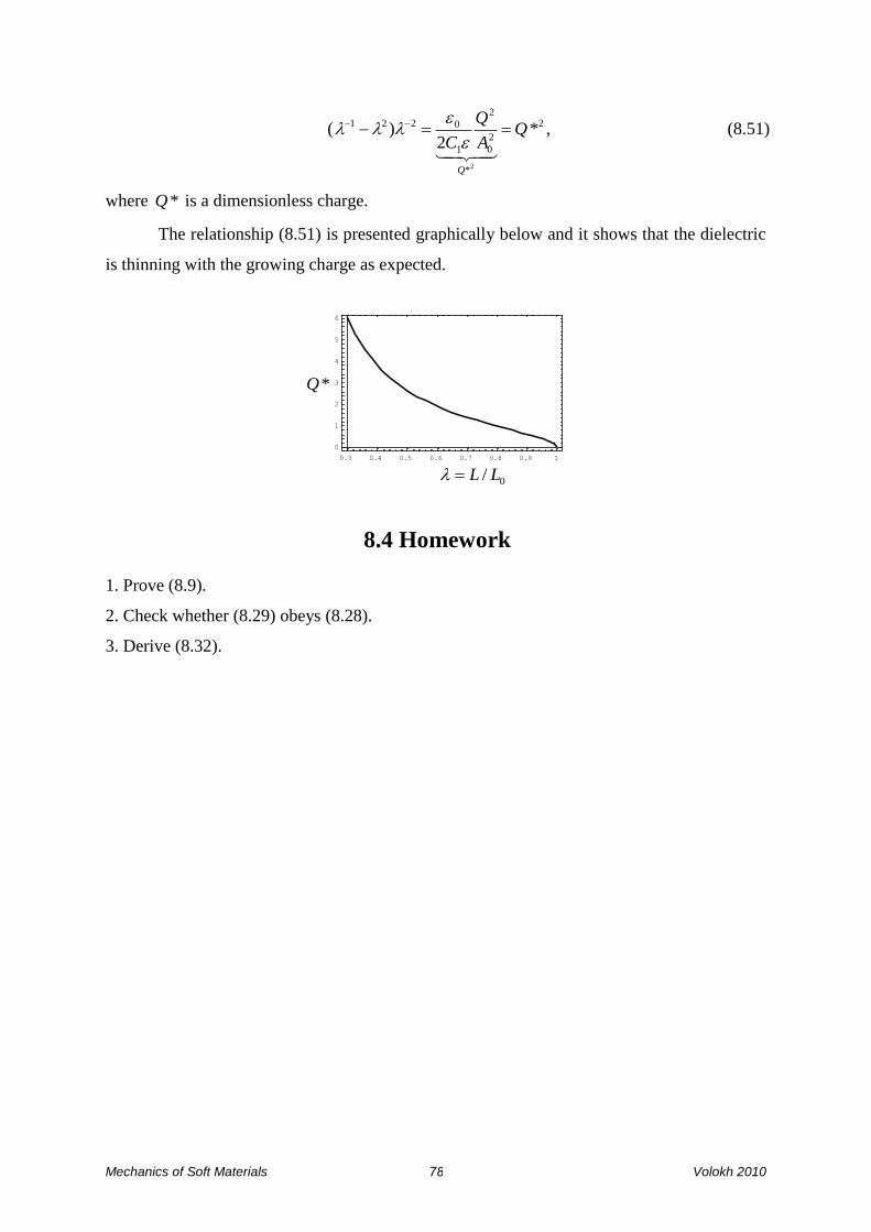
Mechanics of Soft Materials Volokh 2010 78
2
*
2
0
2
1
0221 *2
)(
2
QA
Q
C
Q
, (8.51)
where *Q is a dimensionless charge.
The relationship (8.51) is presented graphically below and it shows that the dielectric
is thinning with the growing charge as expected.
8.4 Homework
1. Prove (8.9).
2. Check whether (8.29) obeys (8.28).
3. Derive (8.32).
0/ LL
*Q
0.3 0.4 0.5 0.6 0.7 0.8 0.9 1
0
1
2
3
4
5
6