Embed Size (px)
Citation preview

1
BAO HUYNH
12524847
PHYSICS 517 QUANTUM MECHANICS II
SPRING 2013
TERM PAPER
‘NON – HILBERTIAN’ QUANTUM
MECHANICS ON THE FINITE
GALOIS FIELD

2
Index table
Section Page
1. Introduction 3
2. Algebraic construction of the
new quantum theory
4
3. Hidden variable theory and
CHSH inequality
5
4. Quantum mechanics on
8
5. Two – particle system in
quantum mechanics
11
6. Contradictions with classical
local hidden variable theory
18
7. CHSH bound
20
8. Conclusion 20
9. Works cited 22

3
1. Introduction
Quantum mechanics, as we have known for the past 88 years, rests upon the Hilbert vector
space. In a recent paper published in January 8th
2013, Lay Nam Chang, Zachary Lewis, Djordje
Minic, and Tatsu Takeuchi from Virginia Tech university proposed the idea of constructing an
alternative ‘Non – Hilbertian’ “discrete quantum mechanics on the vector space over the
finite Galois field ( ) ” (Source 1). This is an attempt to improve our understanding on
mathematical foundations of quantum mechanics. Just as Non – Euclidean geometry has helped
us understood the curvature structure of space – time in general relativity, the replacement of
Hilbert space with the finite Galois field as the space on which quantum state vectors are defined
could potentially lead to invaluable insights into quantum mechanics at its most fundamental
level. However, in order for the new algebraic system defined on to be qualified as a truly
quantum mechanical system, it needs to be shown that “no theory of local hidden variables can
reproduce all the predictions of the system” (Sources 1 and 3). A common way to do this is to
show that our algebraic construction violates the Clause – Horne – Shimony – Holt (CHSH)
inequality which set an upper bound on the correlation between two distant events. If the local
hidden variable, which connect two distant events, really exist then this correlation upper bound
is found to be 2 (Sources 1 and 3). The mathematical structure of quantum mechanics on Hilbert
space forces this upper bound to be √ > 2 which means that quantum mechanics on Hilbert
space violate the CHSH inequality. So, violation of the CHSH inequality is a confirmation test to
show that whether a system is quantum mechanical or not (Source 1). However, our new system
on finite Galois field turns out not to violate the CHSH inequality, and the correlation upper
bound for this system turns out to be the classical hidden variable value 2. Nevertheless, the
authors were able to show some results derived from the mathematical structure of the new
system on that contradicts with the predictions of classical local hidden variables theory. Thus
they conclude that “the new system cannot be fully described by any local hidden variable
theory” (Source 1). Therefore, the new system is qualified as a quantum mechanical system.

4
2. Algebraic construction of the new quantum theory
The heart of this new quantum construction is the idea of replacing the Hilbert space with a finite
field as the ‘space’ in which the N - dimensional state vectors ⟩ of the quantum
system are defined (1). Here according to Galois theorem, is the unique finite field of order q
known as “Galois field GF(q) where q = with p a prime number and n ” (Sources 1 and 2).
When n=1, GF(q) = GF(p) = ( ) (1 and 2). The outcome of a measurement made on
the state ⟩ is defined to be dual vector ⟨ in the dual space . “The probability of obtaining a
result ⟨ when a measurement of a certain observable O is made on the state ⟩ is defined as”:
(⟨ ⟩) ⟨ ⟩
∑ ⟨ ⟩ (1 and 2)
Where the sum in the denominator runs over the set of all possible results of the observable O.
Here, the number ⟨ ⟩ , where ⟨ ⟩ , is defined using the following function:
| | {
(Eqn 1) (1 and 2)
The underline bar is used to denote elements in . The ‘state space’ is given the finite
projective geometry ( ) ( ) ( ) where
( ) “The projective geometry PG(N – 1, F) of an N – vector
space V over a field F is the geometry whose points, lines, planes,… are the vector subspaces of
V of dimensions 1, 2, 3 …” (Source 4). “The group of all possible basis transformations of the
space is the projective linear group ( ) ( ) ( ) where ( ) is the
general linear group of and ( ) is the center of ( )” (Source 1). “The general linear
group ( ) is the group of all non – singular linear transformations of . The
representation of the group ( ) is the group of invertible N N matrices with entries in ”
(Source 1).
The absolute value function defined above for the elements of is the only one which satisfies
the product preserving condition | | | || | required in order for “the probabilities of product
observables on product states to be factorizable into product of individual observable on
individual state” (Source 2)
(⟨ ⟩) (⟨ ⟨ )( ⟩ ⟩)
∑ (⟨ ⟨ )( ⟩ ⟩)
⟨ ⟩⟨ ⟩
∑ ⟨ ⟩⟨ ⟩
⟨ ⟩ ⟨ ⟩
∑ ⟨ ⟩ ⟨ ⟩
⟨ ⟩
∑ ⟨ ⟩
⟨ ⟩
∑ ⟨ ⟩ (⟨ ⟩) (⟨ ⟩) (Sources 1 and 2)
The quantum system built on the above specified algebraic structure is called Galois field
quantum mechanics, abbreviated as GQM. If our GQM model is built over the vector space ,
then we denote it as GQM(N, q). “Spin – like systems with two possible outcomes for the

5
spin operator can be constructed on the vector space as GQM(2, q). Two – particle spin
– like systems can be constructed as GQM(4, q) on the space
”. For each
system of GQM(N, q), we have non – zero quantum states (Source 1). In this paper I will
demonstrate in detail the case q = 2 because the mechanisms of the cases of higher values of q is
exactly the same as that of the case q = 2.
3. Hidden variable theory and CHSH inequality
Einstein, Podolsky, and Rosen proposed a paradox, known collectively as the EPR paradox,
which led them to conclude that quantum theory was incomplete unless a local hidden variable
existed. Their idea became known as the local hidden variable theory (Source 3). The local
hidden variable theory states that distant events have no instantaneous (or faster than light)
effects on local events. “However, in 1964, John Stewart Bell showed that in a Gedanken
experiment of Bohm, no physical theory of local hidden variables can ever reproduce all of the
predictions of quantum mechanics" (Source 3). In 1969, John Clauser, Michael Horne, Abner
Shimony, and Richard Holt proposed an experimental test to confirm Bell’s theorem. This
experiment led directly to the Clauser – Horne – Shimony – Holt inequality (CHSH inequality)
which set an upper bound to how much correlated two distant events could be if local hidden
variable theory were true (Source 3). This upper bound turned out to be 2. Violation of the
CHSH inequality, i.e. a correlation upper bound greater than 2, is a necessary step to show that a
system does not behave according to local hidden variable theory (Source 1). The mathematical
structure of the regular quantum theory on Hilbert space requires this correlation upper bound to
be √ > 2 (Source 1). Therefore, quantum mechanics on Hilbert space violates the CHSH
inequality. This leads to the conclusion that quantum mechanics cannot by described by the local
hidden variable theory. So, in order for an algebraic system to be qualified as a quantum system,
it needs to be shown, either through violation of CHSH inequality or some other way, that no
local hidden variable theory can describe the system (Source 1). This is the argument used in this
paper to show that the quantum system defined over the finite Galois field is indeed a truly
quantum system (Source 1).
In the experiment proposed by Clause, Horne, Shimony, and Holt, a source simultaneously ejects
two identical particles in opposite directions. One particle enters the apparatus A and the other
enters the apparatus B. A and B are two – channel systems where the two channels are +1 and -1.
So, a particle entering an apparatus will have to choose whether to go through channel +1 or -1.
Let a and b be adjustable apparatus parameters for systems A and B, so A(a) and B(b) will have
values depending on which channel the particle decides to go through once it has entered an
apparatus (Source 3). There is a coincidence monitor which increments by 1 every time there is a
pair of particle that have A(a) = B(b). Suppose, the two particles share some common
information, then this common information is the set of locally hidden variables carried within
each particle (Source 3). The set of locally hidden variables are denoted collectively as . So, the
result of channel selection by a particle within an apparatus, either A or B, is described by

6
( ) and ( ). Once again, ( ) and ( ) take on values of depending on which
channel of the apparatus the particle selects (Source 3). “The probability of the result of channel
selection by each particle does not depend on the apparatus parameter a or b because each
particle is ejected from a source which is physically independent from the apparatus. Thus, the
probability of channel selection depends only . Therefore, the probability distribution of
channel selection ( ) is defined over the domain of the common information ” (Source 3).
“The correlation function is defined as ( ) ∫ ( ) ( ) ( )
where is the
domain of (Source 3). Using triangle inequality, we have:
( ) ( ) ∫ ( ) ( ) ( ) ( ) ( )
∫ ( ) ( )
[
( ) ( )] ( ) ( ) (Source 3)
Because A and B takes on values ( ) ( )
So: ( ) ( ) ∫ [ ( ) ( )] ( )
∫ ( ) ( ) ( )
(*)
(Source 3)
The correlation function P takes on values between 0 and 1 with 1indicating 100% correlation
and 0 indicating no correlation. Suppose that ( )
( ) ( ) We can now divide the domain into two parts such that
( ) ( ) , then ∫ ( )
(Source 3). Also, we have:
∫ ( ) ( ) ( )
∫ ( ) ( ) ( )
∫ ( ) ( ) ( )
( ) ∫ ( ) ( ) ( )
(Source 3)
Because: ( ) ( ) ∫ ( ) ( ) ( )
∫ ( )
∫ ( ) ( ) ( )
( ) ( ) ( ) (**) (Source 3)
From (*) and
(**) ( ) ( ) ( ) ( )
{ ( ) ( ) ( ) ( )
( ) ( ) ( ) ( ) (Source 3)
But since: ( ) ( ) ( ) ( ) ( ) ( )
2 ( ) ( )
2 ( ) ( ) ( ) ( ) ( ) ( )
( ) ( ) ( ) ( ) (Source 3)

7
This is the most popular form of the CHSH inequality. From the above derivation, we can see
where the upper bound of 2 came from if a local hidden variable existed. The most common
schematic for the CHSH experiment is shown below:
FIGURE 1. Basic schematic of CHSH experiment. A pair of particles is ejected simultaneously
from a common source S into opposite directions. Each particle will enter a two – channel
system A or B with an adjustable apparatus parameter a or b. A detector is placed in each
channel to detector the particle, detector is used to detect the particle if it enters channel +1 of
the apparatus and detector is used in channel -1 of the apparatus. The coincidence monitor
CM will increment by 1 if the two particles choose the same type of channel (i.e. either both +1
or both -1) in each apparatus (Source 5).
For the quantum system defined on the vector space presented in this paper, the CHSB bound
is not the common value √ for regular quantum system on Hilbert space but turns out to be 2
which is classical hidden variable value (Source 1). However, the authors argued that the
derivation of the CHSH bound value of √ for quantum system in Hilbert space relies heavily
on the inner product operation which the vector space does not have because of the cyclicity
of the Galois field (Source 1). Despite the fact that the quantum system on Galois field does not
violate the CHSH inequality, the authors were able to derive some results that contradict the
predictions of classical hidden variable theory. Therefore, the newly defined quantum system
cannot be described by any theory of hidden variables, and thus is a truly quantum system.
B
8
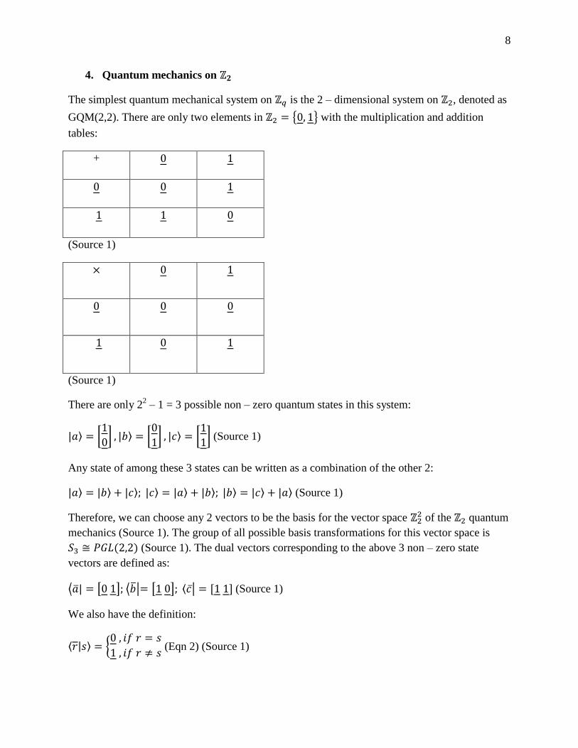
4. Quantum mechanics on
The simplest quantum mechanical system on is the 2 – dimensional system on , denoted as
GQM(2,2). There are only two elements in { } with the multiplication and addition
tables:
+
(Source 1)
(Source 1)
There are only 22 – 1 = 3 possible non – zero quantum states in this system:
⟩ [
] ⟩ [
] ⟩ [
] (Source 1)
Any state of among these 3 states can be written as a combination of the other 2:
⟩ ⟩ ⟩ ⟩ ⟩ ⟩ ⟩ ⟩ ⟩ (Source 1)
Therefore, we can choose any 2 vectors to be the basis for the vector space of the quantum
mechanics (Source 1). The group of all possible basis transformations for this vector space is
( ) (Source 1). The dual vectors corresponding to the above 3 non – zero state
vectors are defined as:
⟨ ̅ [ ] ⟨ ̅| [ ] ⟨ ̅| [ ] (Source 1)
We also have the definition:
⟨ ⟩ {
(Eqn 2) (Source 1)

9
So from (Eqn 1) and (Eqn 2) ⟨ ⟩ (Eqn 3) (source 1)
Just like for the vector space , we can choose any 2 of the above 3 non – zero dual vectors to
form the basis for the dual vector space ( ) . We have 3 dual vectors, and we need to select 2
of them to form the basis for the dual space, so have ( ) possible selections for the basis.
An observable for this quantum system is defined to be one the 3 possible selections for the pair
of dual vectors above. So, we have:
⟨ ⟨ where ⟨ ⟨ are two of the 3 non – zero dual vectors
⟨ ⟨ ⟨ defined above (Source 1.)
Also, ⟨ represents the outcome +1 and ⟨ represents the outcome of -1 when observable is
measured and (Source 1).
Since we have 3 possible selections of the pair of dual vectors, we have 3 observables
. Let us denote (Source 1).
X, Y, and Z transform into each other under the permutation group
( ) ( ) ( ) ( ) ( ) ( ) where the cycle ( ) represents the identity
permutation, i.e. no permutation, which is trivial so we will not consider it here (Source 1). In
this situation, ( ) means a gets changed into b, b gets changed into c, and c gets changed into
a; so the subscript indices of an observable, say , will be changed into bc under the cycle
( ). So, ( ) . Below is the list of all non – trivial transformations of the
observables X, Y, and Z (Source 1):
X Y Z
( ) -Y -X -Z
( ) -X -Z -Y
( ) -Z -Y -X
( ) +Y +Z +X
( ) +Z +X +Y

10
“The six cycles in can be mapped into the six rotations in the dihedral group which rotate
the triangle abc in the figure below into itself.” (Source 1)
FIGURE 2. The six rotation axes that map the triangle onto itself (Source 1)
As mentioned previously, in this quantum mechanics, there are only two eigenvalues for
all the observables in this system. So, let us take the observable for an example, it is defined
as {⟨ ⟨ }. When the observable operates on a certain state ⟩, the outcome value
could only be +1 or -1, with ⟨ representing ⟨ and ⟨ representing ⟨ . So, the probability of
getting an outcome of +1 when operates on ⟩ is:
( ⟨ ⟩) ⟨ ⟩
⟨ ⟩ ⟨ ⟩
⟨ ⟩
⟨ ⟩ |⟨ | ⟩| (Eqn 4)
Where ⟨ ⟩ and |⟨ | ⟩| are calculated according to (Eqn 3):
⟨ ⟩ |⟨ | ⟩| (Eqn 5)
And the outcome expectation value of the observable when operating on ⟩ is:
⟨ ⟩ ( ) ( ⟨ ⟩) ( ) ( ⟨ ⟩) (Eqn 6)
Since we only have 3 states ⟩, ⟩, ⟩, the outcome probabilities and when the observable
operates on them are calculated based on (Eqn 4) and (Eqn 5) as follows:
( ⟨ ⟩) ⟨ ⟩
⟨ ⟩ |⟨ | ⟩| (Source 1)
( ⟨ ⟩) |⟨ | ⟩|
⟨ ⟩ |⟨ | ⟩| (Source 1)
( ⟨ ⟩) ⟨ ⟩
⟨ ⟩ |⟨ | ⟩| (Source 1)

11
( ⟨ ⟩) |⟨ | ⟩|
⟨ ⟩ |⟨ | ⟩| (Source 1)
( ⟨ ⟩) ⟨ ⟩
⟨ ⟩ |⟨ | ⟩|
(Source 1)
( ⟨ ⟩) |⟨ | ⟩|
⟨ ⟩ |⟨ | ⟩|
(Source 1)
The expectation values of when operating on ⟩, ⟩, ⟩ are calculated based on (Eqn 6) as
follow:
⟨ ⟩ ( ) ( ) ( ) ( ) (Source 1)
⟨ ⟩ ( ) ( ) ( ) ( ) (Source 1)
⟨ ⟩ ( ) (
) ( ) (
) (Source 1)
Like wise we can compute the outcome probabilities and expectation values for and , and
the list of all the probabilities and expectation values are shown below:
Observable State P(+) P(-) Expectation
Value
⟩ 0 1 -1
⟩ 1 0 +1
⟩
0
⟩
0
⟩ 0 1 -1
⟩ 1 0 +1
⟩ 1 0 +1
⟩
0
⟩ 0 1 -1
(Source 1)
5. Two – particle system in quantum mechanics
Each particle in quantum mechanics exist in the space , so the space for 2 – particle system
in quantum mechanics is . This Galois quantum mechanics for the 2 – particle system is
denoted as GQM(4, 2). There are 24 – 1 = 15 non – zero quantum states which divide themselves
into 9 pure states and 6 entangled states. The nine pure states are defined as follow:
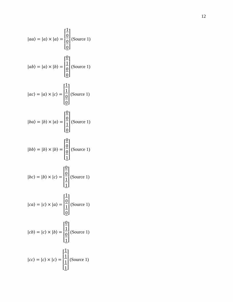
12
⟩ ⟩ ⟩
[
]
(Source 1)
⟩ ⟩ ⟩
[
]
(Source 1)
⟩ ⟩ ⟩
[
]
(Source 1)
⟩ ⟩ ⟩
[
]
(Source 1)
⟩ ⟩ ⟩
[
]
(Source 1)
⟩ ⟩ ⟩
[
]
(Source 1)
⟩ ⟩ ⟩
[
]
(Source 1)
⟩ ⟩ ⟩
[
]
(Source 1)
⟩ ⟩ ⟩
[
]
(Source 1)

13
The six entangled states are defined as follow:
⟩ ⟩ ⟩ ⟩
[
]
(Source 1)
This state transforms into itself under all permutations of
The other 5 entangled states are:
( )⟩ ⟩ ⟩ ⟩
[
]
(Source 1)
( )⟩ ⟩ ⟩ ⟩
[
]
(Source 1)
( )⟩ ⟩ ⟩ ⟩
[
]
(Source 1)
( )⟩ ⟩ ⟩ ⟩
[
]
(Source 1)
( )⟩ ⟩ ⟩ ⟩
[
]
(Source 1)
Similar to the case of 1 – particle system, we can define dual vectors in the dual space ( ) for
the 2 – particle system. However, we can only define the dual vectors corresponding to the 9
pure state vectors:
⟨ ⟨ [ ] (Source 1)
⟨ | ⟨ | [ ] (Source 1)
⟨ ⟨ [ ] (Source 1)

14
⟨ ⟨ [ ] (Source 1)
⟨ | ⟨ | [ ] (Source 1)
⟨ ⟨ [ ] (Source 1)
⟨ ⟨ [ ] (Source 1)
⟨ | ⟨ | [ ] (Source 1)
⟨ ⟨ [ ] (Source 1)
Also similar to the case of 1 – particle system, we can define the observables for the 2 – particle
system as the selections of basis for the dual space ( ) :
{⟨ | ⟨ | ⟨ ⟨ ⟨ | ⟨ | ⟨ ⟨ } where (Source 1)
So there are a total of 9 observables. Suppose we have a state
⟩ ⟩ ⟩ ⟩ ( ⟩) ( ⟩)
So an operator of a 2 – particle system state consists of one operator on the state of the 1 first
particle, and another operator on the state of the second particle. Let the set of operators on the
first particle be and the set of operators on the second operators be where
.
Suppose we have a 2 – particle operator {⟨ | ⟨ | ⟨ ⟨ ⟨ | ⟨ | ⟨ ⟨ }
operating on a state ⟩ ⟩ ⟩. The vector ⟨ represent the +1 outcome and ⟨
represents the -1 outcome when is measured, but ⟨ represents +1 when is measured
and ⟨ represents -1 when is measured. So, ⟨ ⟨ ⟨ ⟨ for the first particle and
⟨ ⟨ ⟨ ⟨ for the second particle ⟨ ⟨ ⟨ ⟨ ⟨
⟨ ⟨ ⟨ . Probabilities for the outcomes are calculated as follow:
( ⟨ ⟩) ⟨ ⟩
∑ ⟨ ⟩
(⟨ ⟨ )( ⟩ ⟩)
∑ (⟨ ⟨ )( ⟩ ⟩)
⟨ ⟩ ⟨ ⟩
∑ ∑ ⟨ ⟩ ⟨ ⟩
⟨ ⟩
⟨ ⟩ ⟨ ⟩
⟨ ⟩
⟨ ⟩ ⟨ ⟩ ( ⟨ ⟩) ( ⟨ ⟩) (Eqn 7)
Similarly,
( ⟨ ⟩) ( ⟨ ⟩) ( ⟨ ⟩)
( ⟨ ⟩) ( ⟨ ⟩) ( ⟨ ⟩)
( ⟨ ⟩) ( ⟨ ⟩) ( ⟨ ⟩)

15
( ⟨ ⟩) ( ⟨ ⟩) ( ⟨ ⟩)
The outcome expectation when operates on ⟩ ⟩ ⟩ is calculated as:
⟨ ⟩ ∑ ( ⟨ ⟩) ∑ ( ⟨ ⟩) ( ⟨ ⟩)
(∑ ( ⟨ ⟩)) (∑ ( ⟨ ⟩)) ⟨ ⟩ ⟨ ⟩
(Eqn 8)
Based on the above rules specified in (Eqn 7) and (Eqn 8), we can calculate all the outcome
probabilities and expectation values for all the 9 observables of the 2 – particle system. The
results are tabulated below:
Observable State P(+ +) P(+ -) P(- +) P(- -) Expectation
Value
⟩ 0
0 -1
( )⟩
0
( )⟩
0 0
+1
( )⟩ 0
( )⟩
0
( )⟩
0
(Source 1)
Observable State P(+ +) P(+ -) P(- +) P(- -) Expectation
Value
⟩
0
( )⟩
( )⟩
( )⟩
( )⟩
( )⟩
(Source 1)

16
Observable State P(+ +) P(+ -) P(- +) P(- -) Expectation
Value
⟩
( )⟩ 0
( )⟩
0
( )⟩
+1
( )⟩
( )⟩
(Source 1)
Observable State P(+ +) P(+ -) P(- +) P(- -) Expectation
Value
⟩
( )⟩
( )⟩
( )⟩
( )⟩
( )⟩
(Source 1)
Observable State P(+ +) P(+ -) P(- +) P(- -) Expectation
Value
⟩
( )⟩
( )⟩
( )⟩
( )⟩
( )⟩

17
Observable State P(+ +) P(+ -) P(- +) P(- -) Expectation
Value
⟩
0
( )⟩
( )⟩
( )⟩
( )⟩
( )⟩
(Source 1)
Observable State P(+ +) P(+ -) P(- +) P(- -) Expectation
Value
⟩
0
( )⟩
( )⟩
( )⟩
( )⟩
( )⟩
(Source 1)

18
Observable State P(+ +) P(+ -) P(- +) P(- -) Expectation
Value
⟩
( )⟩
( )⟩
( )⟩
( )⟩
( )⟩
(Source 1)
Observable State P(+ +) P(+ -) P(- +) P(- -) Expectation
Value
⟩
( )⟩
( )⟩
( )⟩
( )⟩
( )⟩
(Source 1)
6. Contradictions with classical local hidden variable theory
According to the above probabilities tables, ( ⟨ ⟩) ( ⟨ ⟩) ( ⟨ ⟩)
The interpretation of the above equation is that for the 2 particles in the state ⟩, if the outcome
value when the operator operates on the 1st particle of the state ⟩ is +1, i.e. , then
the outcome value when the operator operates on the 2nd
particle of the state ⟩ CANNOT be
-1, i.e. , which implies that MUST BE +1 because it can only be either +1 or -1. So,
the probability equation ( ⟨ ⟩) says that
(I). Conversely, ( ⟨ ⟩) also says that .
Similarly from the probability ( ⟨ ⟩) we have (II). And
from ( ⟨ ⟩) we have (III)

19
From (I) (II) and (III), we have the line of implication below:
()
Which means that (IV)
If a classical local hidden variable theory were true for the this quantum system, the line of
implication () must be true, hence the implication (IV) must be true.
But we also have from the first probability table above that ( ⟨ ⟩) which says
which contradicts the implication (IV). So, we
have just seen one prediction of our quantum system that contradicts the prediction of a local
hidden variable theory if it were true on our system. Therefore, we can conclude that no local
hidden variable theory can reproduce all the predictions of our quantum mechanical system on
. Therefore, the algebraic system constructed on the space
is qualified as a truly quantum
mechanical system.
Just to further solidify our reasoning, another contradiction with local hidden variable theory will
be shown below:
From ( ⟨ ⟩) , we have
From ( ⟨ ⟩) , we have
From ( ⟨ ⟩) , we have
From ( ⟨ ⟩) , we have
So a classical hidden variable theory would predict ()
From ( ⟨ ⟩) , we have ()
From () and (), classical hidden variable theory would predict which
is equivalent to ( ⟨ ⟩)
So, classical hidden variable theory predicts that ( ⟨ ⟩)
But from our probabilities tables we have ( ⟨ ⟩)
Therefore, the prediction of our quantum system in this case, once again, contradicts the
prediction of local hidden variable theory. Hence, our construction is truly quantum.

20
7. CHSH bound
Let and be observables that operates on the states of the particles respectively,
where take on values 1 and 2 since there are only 2 particle in our system (Source 1).
Then the CHSH correlation function for a certain 2 – particle state ⟩ is defined as:
⟨ ⟩ ⟨ ⟩ ⟨ ⟩ ⟨ ⟩ ⟨ ⟩ where ⟨ ⟩ is just the
expectation value of the observable when it operates on ⟩ (Source 1)
Going through the list of all the 9 observables and all the states of this 2 – particle system, the
authors obtained the following maximum correlation bounds for the state ⟩
⟨ ⟩ ⟨ ⟩ where once again
(Source 1)
The results obtained for other observables and other states are all
. Therefore, the upper
bound for the correlation of our 2 – particle system is 2, which is the CHSH limit for classical
hidden variable theory (Source 1).
However, the fact that our system does not violate the CHSH bound does not mean that our
system could be fully described by a local hidden variable theory. The contradictions we derived
in previous section already showed that this is not the case.
So, violating the CHSH bound implies violating local hidden variable theory. But not violating
CHSH bound DOES NOT imply not violating local hidden variable theory.
8. Conclusion
In our construction in this paper the dual vector ⟨ that we defined represents an outcome value
of either +1 or -1 when an observable O is measured for a certain state ⟩. It does not, however,
represent the conjugate transpose of a quantum state. Therefore, ⟨ ⟩ is an outcome value of the
observable O when it is measured on ⟩ NOT the inner product between two states. Hence,
(Eqn 2) and (Eqn 3) do not define an inner product. In fact, an inner product is impossible for our
system because the Galois field is cyclic (Source 1). It is because of this lack of inner product
that our system fails to violate the CHSH bound of 2 for classical hidden variable theory (Source
1). Because the authors argued that the derivation of the CHSN bound value of √ for the
regular quantum mechanics on Hilbert space involves extensive usage of inner product, which is
perfectly defined in Hilbert space (Source 1).
Also, the fact that the observables defined in our system can transform into each
other under the permutation group ( ) ( ) ( ) ( ) ( ) ( ) and the fact they
can only take values of , imply that these observables behave similarly to the spin operator in

21
Hilbert space quantum mechanics (Source 1). So we can think of our set of observables as the
Galois field analog of the Hilbert space quantum mechanics spin operator.
Other than that, I think we have successfully ‘synthesized’ a mini quantum mechanical model on
the finite Galois field . I think that the idea of removing quantum mechanics from the Hilbert
space and trying to rebuild it on a different algebraic structure is a uniquely interesting idea.
Because it reveals some unknown aspects of the mathematical foundations of quantum theory.
For example, only by examining the Galois field, are we able to find out the role of the inner
product in producing the CHSH limit of √ for quantum theory on Hilbert space. There are
many more yet to be discovered algebraic aspects of quantum theory that the new quantum idea
promises to offer. In this respect, I think the authors of this Galois field quantum mechanics have
found a new route to better understanding of quantum theory.

22
Works Cited
1. Chang, Lay Nam, Zachary Lewis, Djordje Minic, and Tatsu Takeuchi.
“Spin and Rotations in Galois Field Quantum Mechanics”. Cornell University
Library, 2013. arXiv:1206.0064v3 [quant – ph]. Web. 6 January 2013.
<http://arxiv.org/pdf/1206.0064v3.pdf>
2. Chang, Lay Nam, Zachary Lewis, Djordje Minic, and Tatsu Takeuchi.
“Galois Field Quantum Mechanics”. Cornell University Library, 2013.
arXiv:1205.4800v2 [quant – ph]. Web. 6 January 2013.
<http://arxiv.org/pdf/1205.4800v2.pdf>
3. Clauser, John F., Michael A. Horne, Abner Shimony, Richard A. Holt.
“Proposed Experiment To Test Local Hidden – Variables Theories”. Physical
Review Letters. Volume 23, Number 15. 13 October 1969: 880 – 4. Print.
4. Cameron, Peter. “Projective Spaces”. Home page.
<http://www.maths.qmul.ac.uk/~pjc/pps/pps1.pdf>. Web. 4 June 2013.
5. Wikipedia. “CHSH Inequality”. Wikipedia, 2013. Web. 4 June 2013.
<http://en.wikipedia.org/wiki/CHSH_inequality>

23


![Part II | Galois Theorydec41.user.srcf.net/notes/II_M/galois_theory_thm_proof.pdf · Normal and Galois extensions, automorphic groups. Fundamental theorem of Galois theory. [3] Galois](https://img.pdfslide.net/doc/110x75/5f3b019b8ccd1673676b3f72/part-ii-galois-normal-and-galois-extensions-automorphic-groups-fundamental-theorem.jpg)