Applied Mathematics and Mechanics (English Edition), 2007, 28(8):1019–1028c©Editorial Committee of Appl. Math. Mech., ISSN 0253-4827

Mechanism of transition in a hypersonic sharp cone boundary layerwith zero angle of attack ∗

DONG Ming (��), LUO Ji-sheng (���)

(Department of Mechanics, Tianjin University, Tianjin 300072, P. R. China)

(Contributed by LUO Ji-sheng)

Abstract Firstly, the steady laminar flow field of a hypersonic sharp cone boundarylayer with zero angle of attack was computed. Then, two groups of finite amplitude T-Swave disturbances were introduced at the entrance of the computational field, and thespatial mode transition process was studied by direct numerical simulation (DNS) method.The mechanism of the transition process was analyzed. It was found that the change ofthe stability characteristics of the mean flow profile was the key issue. Furthermore, thecharacteristics of evolution for the disturbances of different modes in the hypersonic sharpcone boundary layer were discussed.

Key words sharp cone boundary layer, stability, transition, zero angle of attack

Chinese Library Classification O357.412000 Mathematics Subject Classification 76F06Digital Object Identifier(DOI) 10.1007/s10483-007-0804-2

Introduction

Transition and turbulence problems have been a hot point of research in the branch of fluidmechanics for a long period. Wall turbulence, especially the boundary layer turbulence, is themost familiar turbulent status in both engineering and nature. As the computer technology de-veloped, direct numerical simulation (DNS) has become a powerful tool in turbulence research.Most of the earlier numerical simulations were based on incompressible flow, and temporalmode was frequently employed. When compared to the spatial mode, temporal mode takesmuch less computational resources, but the hypothesis of periodicity in stream wise direction issupposed in such a way that temporal mode can only solve some simple cases. For a complexflow such as sharp cone and blunt body, this method may not make sense. For the develop-ment of aviation technology, the study of transition forecast and turbulence characteristic incompressible flow is considered to be very important. Most of the present DNS of compressibleflow are based on flat boundary layer, but in engineering, investigations of flat boundary layermay not be enough. Dong Ming, et al.[1] studied the characteristics of the evolution of laminardisturbances in supersonic sharp cone boundary layer with zero angle of attack, however, thestudy did not simulate the process of transition, and further investigation on the transitionprocess of sharp cone boundary layer needs to be developed.

The traditional description of transition process is as follows: the transition begins with theblowup of the disturbances, then as a result of the nonlinear effect, high-order harmonious wouldbe generated, the flow becomes highly complex, and finally, turbulence appears. However, inthe study of the transition mechanism of incompressible channel flow, Wang Xinjun, et al.[2]

pointed out that the traditional description could not explain the “breakdown” process in

∗ Received May 10, 2007; Revised Jun. 21, 2007Project supported by the National Natural Science Foundation of China (Key Program)(No. 10632050)Corresponding author LUO Ji-sheng, E-mail: jsluo@tju.edu.cn

1020 DONG Ming and LUO Ji-sheng

transition. They found that the change of stability characteristic in mean flow may act a keyrole in “breakdown” process. Later, Huang Zhangfeng, et al.[3] and Cao Wei, et al.[4] arrivedat similar conclusions for the study of transition on flat supersonic boundary layer with theoncoming flow of Mach number 4.5, using temporal and spatial mode, respectively. It wasfound that although the most unstable wave in laminar flow is the wave of the second mode, itis the first mode that plays a key role in the transition process. In this article, the transitionmechanism of a hypersonic sharp cone boundary layer with the oncoming flow Mach number6, semi-angle 5◦, and zero angle of attack was studied by spatial mode.

y Computational domain

xφ

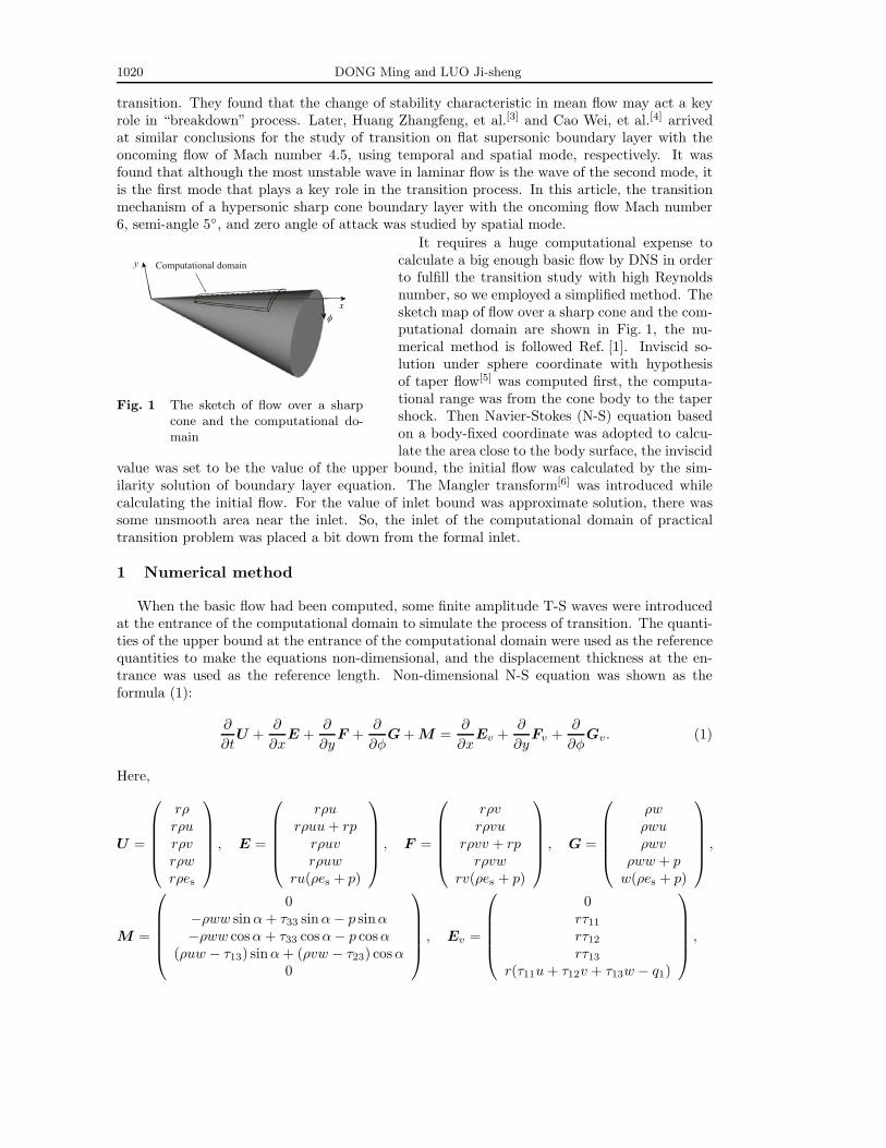
Fig. 1 The sketch of flow over a sharpcone and the computational do-main

It requires a huge computational expense tocalculate a big enough basic flow by DNS in orderto fulfill the transition study with high Reynoldsnumber, so we employed a simplified method. Thesketch map of flow over a sharp cone and the com-putational domain are shown in Fig. 1, the nu-merical method is followed Ref. [1]. Inviscid so-lution under sphere coordinate with hypothesisof taper flow[5] was computed first, the computa-tional range was from the cone body to the tapershock. Then Navier-Stokes (N-S) equation basedon a body-fixed coordinate was adopted to calcu-late the area close to the body surface, the inviscid

value was set to be the value of the upper bound, the initial flow was calculated by the sim-ilarity solution of boundary layer equation. The Mangler transform[6] was introduced whilecalculating the initial flow. For the value of inlet bound was approximate solution, there wassome unsmooth area near the inlet. So, the inlet of the computational domain of practicaltransition problem was placed a bit down from the formal inlet.

1 Numerical method

When the basic flow had been computed, some finite amplitude T-S waves were introducedat the entrance of the computational domain to simulate the process of transition. The quanti-ties of the upper bound at the entrance of the computational domain were used as the referencequantities to make the equations non-dimensional, and the displacement thickness at the en-trance was used as the reference length. Non-dimensional N-S equation was shown as theformula (1):

∂

∂tU +

∂

∂xE +

∂

∂yF +

∂

∂φG + M =

∂

∂xEv +

∂

∂yFv +

∂

∂φGv. (1)

Here,

U =

⎛⎜⎜⎜⎜⎝

rρrρurρvrρwrρes

⎞⎟⎟⎟⎟⎠

, E =

⎛⎜⎜⎜⎜⎝

rρurρuu + rp

rρuvrρuw

ru(ρes + p)

⎞⎟⎟⎟⎟⎠

, F =

⎛⎜⎜⎜⎜⎝

rρvrρvu

rρvv + rprρvw

rv(ρes + p)

⎞⎟⎟⎟⎟⎠

, G =

⎛⎜⎜⎜⎜⎝

ρwρwuρwv

ρww + pw(ρes + p)

⎞⎟⎟⎟⎟⎠

,

M =

⎛⎜⎜⎜⎜⎝

0−ρww sin α + τ33 sin α − p sinα−ρww cosα + τ33 cosα − p cosα

(ρuw − τ13) sinα + (ρvw − τ23) cosα0

⎞⎟⎟⎟⎟⎠

, Ev =

⎛⎜⎜⎜⎜⎝

0rτ11

rτ12

rτ13

r(τ11u + τ12v + τ13w − q1)

⎞⎟⎟⎟⎟⎠

,

Transition of boundary layer on hypersonic sharp cone 1021

Fv =

⎛⎜⎜⎜⎜⎝

0rτ21

rτ22

rτ23

r(τ21u + τ22v + τ23w − q2)

⎞⎟⎟⎟⎟⎠

, Gv =

⎛⎜⎜⎜⎜⎝

0τ31

τ32

τ33

τ31u + τ32v + τ33w − q3

⎞⎟⎟⎟⎟⎠

,

es =12(u2 + v2 + w2) +

p

(γ − 1)ρ,

τ11 =μ

Re

(2∂u

∂x− 2

3∇ · u

), τ12 = τ21 =

μ

Re

(∂u

∂y+

∂v

∂x

), τ22 =

μ

Re

(2∂v

∂y− 2

3∇ · u

),

τ13 = τ31 =μ

Re(∂w

∂x+

∂u

r∂φ− w

rsin α), τ23 = τ32 =

μ

Re(∂w

∂y+

∂v

r∂φ− w

rcosα),

τ33 = 2μ

Re

(∂w

r∂φ+

u

rsin α+

v

rcosα

)− 2

3μ

Re∇ · u, ∇ · u=

∂u

∂x+

∂v

∂y+

∂w

r∂φ+

u sinα

r+

v cosα

r,

q1 = − k

(γ − 1)M2RePr

∂T

∂x, q2 = − k

(γ − 1)M2RePr

∂T

∂y, q3 = − k

(γ − 1)M2RePr

∂T

r∂φ,

where, r = x sin α + y cosα is the distance from the certain point to the axes of the cone;u = (u, v, w) are the stream wise, normal wise and span wise velocities, respectively; p, T, ρ arethe pressure, temperature and density, respectively; q1, q2, q3 are the heat fluxes; Re is Reynoldsnumber; Pr is Prandtl number.

The flow condition in the numerical simulation was corresponded to the air at a height of10 000 m, the oncoming flow Mach number was set to be 6, the temperature was set to be 223.3K, and the semi-angle was set to be 5◦ , then the shock angle of the taper shock at the frontof the cone would be 10.637◦. Then the Mach number would be 5.773 behind the taper shockwave. The Reynolds number of the entrance of the computational domain was set to be 50 000,the correspondence x value would be 1.23 m. The displacement thickness of the boundary layerat the entrance, δ, was 0.87 mm. Then the value of the Mach number of the upper bound ofthe computational domain using ideal gas equation group and taper flow hypothesis was foundto be 5.585.

In this article, the 5th order upwind difference scheme (2) was used for the nonlinear term,the 6th order center difference scheme (3) was used for the viscous term, and 2nd-order Runge-Kutta method was used in time direction.⎧⎪⎪⎨

⎪⎪⎩

∂f+j

∂x= (− 1

20fj+2 +

12fj+1 +

13fj − fj−1 +

14fj−2 − 1

30fj−3)/dx,

∂f−j

∂x= (

130

fj+3 − 14fj+2 + fj+1 − 1

3fj − 1

2fj−1 +

120

fj−2)/dx,

(2)

∂fj

∂x= (

34(fj+1 − fj−1) − 3

20(fj+2 − fj−2) +

160

(fj+3 − fj−3))/dx. (3)

All the variables were given at the entrance and the upper bound, the fringe method was em-ployed at the outlet bound, at wall of the cone, no-slip condition was used, and the temperaturewas set to be 1 557.8 K, period boundary condition was used at span wise.

During simulation, the uniform meshes were used in x- and φ direction; whereas non-uniformmeshes were used in y-direction, the coordinate of grid points were determined by y = yn(ebη −1)/(eb − 1) , where b = 6.0, and η�0�1, uniform variation.

2 Numerical results and discussions

The method of introducing some finite amplitude T-S waves at the entrance of the flow fieldwas adopted, to investigate the characteristic of transition. Because many unstable mode waves

1022 DONG Ming and LUO Ji-sheng

exist in hypersonic flow, the result of linear stability theory is that, the second mode wave isthe most unstable 2-D wave, whereas the first mode wave, which is similar to the square modein unstable flow, is the most unstable 3-D wave. In order to study the effect of the two modedisturbances in transition, the first mode and the second mode wave was selected as the maininitial disturbance in computing, respectively, especially, the evolution of them in transitionwas investigated. The computational domain was 250δ × 18δ × 14.6◦ and 200δ × 18δ × 14.6◦,respectively, and the number of grid was 1251 × 81 × 101 and 1001 × 81 × 101, respectively.

When investigating the evolution of the disturbances, the disturbances of the velocity, tem-perature and pressure introduced at the entrance were expressed as

(u′, v′, w′, t′, p′)T = a[(u, v, w, t, p)Tei(αx+βz−ωt) + c.c.], (4)

where u, v, w, t, p are the normalization eigenfunction solutions of the linear disturbance equa-tions, which depend on y; c.c. is the conjugate complex; a is the amplitude; ω is the frequency;α is complex number, whose real part represents the stream wise wave number, the oppositenumber of whose imaginary part represents the rate of growth; and β is real number, whichrepresents the span wise wave number; z = φr is the span wise arc length.

Firstly, we take some analysis in Case I. Three T-S waves, whose amplitudes were equal to0.05, were introduced at the entrance of the computational domain, where disturbance I was2-D grow-up wave, which was selected as the most unstable first mode 2-D wave, disturbancesII and III were 3-D waves, the eigenvalues of which were shown in Table 1.

Table 1 Eigenvalues of T-S wave

ω αr −αi β

Disturbance I 0.512 513 0.593 796 0.003 237 0.0Disturbance II 0.512 513 0.602 787 0.010 920 0.4Disturbance III 1.025 026 1.149 153 −0.002 54 0.6

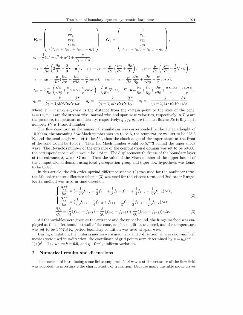
The computation process proceeds until the flow is stable statistically. The evolution ofwall friction coefficient was shown in Fig. 2. At the beginning, the friction coefficient descendedappreciably, and ascended sharply at the place of about x = 100, and then began to descendgently at the place of x = 160. These changes reflected the whole process of the transition fromlaminar to turbulence, and the positions of the beginning and ending of the breakdown processcould be fixed roughly. The evolution of root-mean-square of the perturbation velocity at theplace of y = 0.294 was shown in Fig. 3. Considering that the density varies in compressible flow,the evolution of mean perturbation kinetic energy k = ρu′

iu′i

2 was shown in Fig. 4 ulteriorly. Theevolution also reflected the whole process of transition, the only fact was that the beginningand ending points of the sharp raise in the curves, were a bit ahead of that in Fig. 2. Thereason was that the wall friction coefficient was related to the shape of average flow, whereasthe perturbation kinetic energy was related to the perturbation velocity and the modificationof the average flow was aroused from the perturbation velocity. Therefore, there may be a lagon the variation of the mean flow. And, a noticeable fact was that, considering the effect ofthe density, there were some differences in the distribution between the perturbation kineticenergy and the root-mean-square, especially at the point when x > 110. The reason being themodification of the mean density section. This again means there was a lag on the modificationof the average section compared to the perturbation velocity. At the same time, from thedistribution of derivative of the perturbation kinetic energy shown in Fig. 4, it could be seenthat it was at x = 100 where the perturbation kinetic energy reached the maximum value.

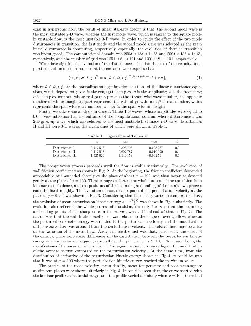
The profiles of the mean velocity, mean density, mean temperature and root-mean-squareat different places were shown ulteriorly in Fig. 5. It could be seen that, the curve started withthe laminar profile at its initial stage; and the profile varied definitely when x = 100; there had

Transition of boundary layer on hypersonic sharp cone 1023

0.0009

0.0006

0.0003

0.00000 50 100 150 200 250

x

cf

Fig. 2 Evolution of friction coefficient inCase I

0.00045

0.00030

0.00015

0.000000 50 100 150 200 250

x

Vrms'

Fig. 3 Evolution of root-mean-square velocityin Case I

0.003

0.002

0.001

0.0000 50 100 150 200 250

x

k

0.0002

0.0001

0.0000

dk/d

x

kdk/dx

0.0001

Fig. 4 Evolution of perturbation kinetic energy and its variance ratio

x = 0x = 100x = 130x = 160x = 230x = 250

x = 0x = 100x = 130x = 160x = 230x = 250

x = 0x = 100x = 130x = 160x = 230x = 250

x = 0x = 100x = 130x = 160x = 230x = 250

4

3

2

1

0

y

0.0 0.2 0.4 0.6

(a) Mean velocity

0.8 1.0u

4

3

2

1

0

y

0.2 0.4 0.6

(b) Mean density

0.8 1.0ρ

4

3

2

1

0

y

1 2 3 4

(c) Mean temperature

5 6T

4

3

2

1

0

y

0.0000 0.0001 0.0002

(d) Root-mean-square velocity

0.0003 0.0004V'rms

Fig. 5 The variation process of mean profile from laminar to turbulence

1024 DONG Ming and LUO Ji-sheng

been a inflexion on mean velocity profile at the point when x = 130, other quantities also variedevidently; when the value increased to x = 160, the inflexion of mean velocity moved upward;and then, from the point, where x = 230, the inflexion disappeared; all quantities showed aslight variation, which meant that the transition process had been completed. This variationof the quantities reflected the whole process of transition: at the state of laminar and after thetransition, the profile varies slowly, but at the state of breakdown in transition, the inflexion ofthe mean velocity profile may come out, and the profile would transform to turbulent profilerapidly. In Fig. 2, the transition had already finished at the point, where x = 160, but inFig. 5, the profile at this place was entirely different from the turbulent profile, the inflexionstill existed. The reason is that, although the ending of transition means it is in turbulent state,the turbulence is not fully developed, this needs an additional process.

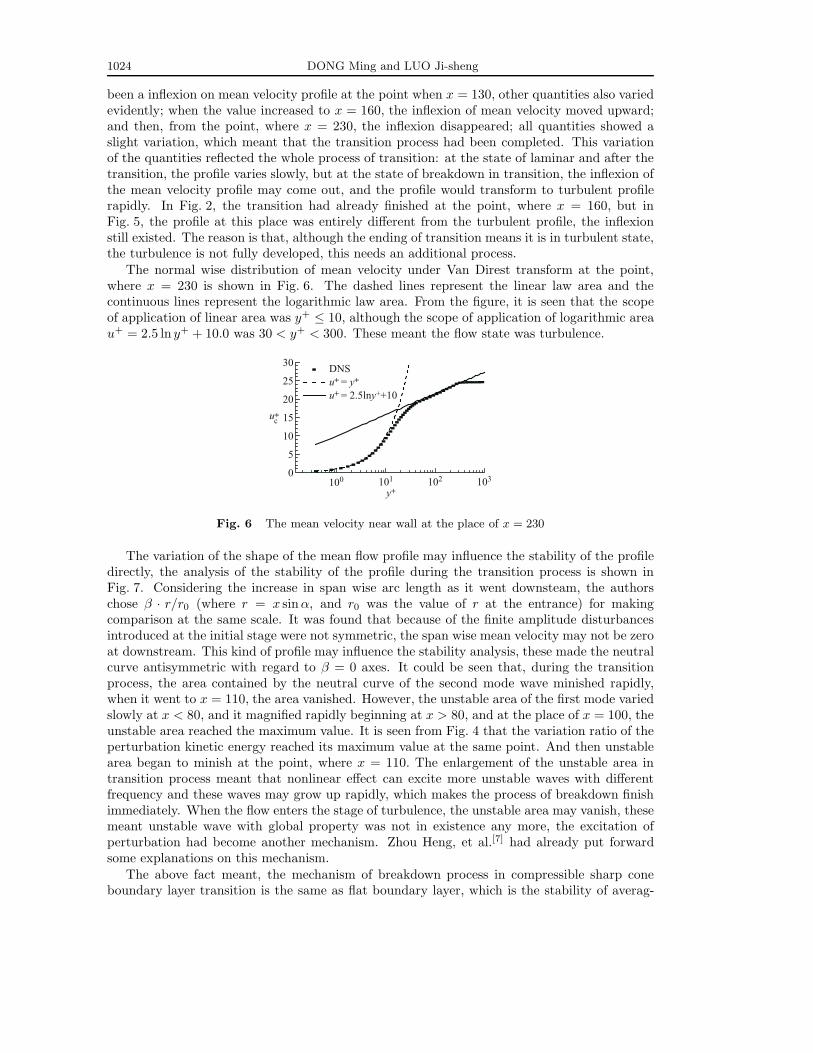
The normal wise distribution of mean velocity under Van Direst transform at the point,where x = 230 is shown in Fig. 6. The dashed lines represent the linear law area and thecontinuous lines represent the logarithmic law area. From the figure, it is seen that the scopeof application of linear area was y+ ≤ 10, although the scope of application of logarithmic areau+ = 2.5 ln y+ + 10.0 was 30 < y+ < 300. These meant the flow state was turbulence.

30

25

20

15

10

5

0

u+c

100 101 102 103

y+

DNSu+ = y+

u+ = 2.5lny++10

Fig. 6 The mean velocity near wall at the place of x = 230

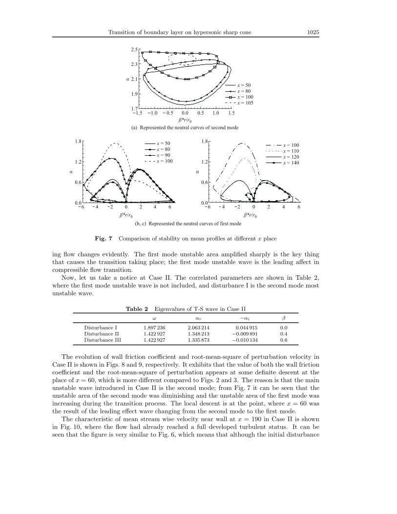
The variation of the shape of the mean flow profile may influence the stability of the profiledirectly, the analysis of the stability of the profile during the transition process is shown inFig. 7. Considering the increase in span wise arc length as it went downsteam, the authorschose β · r/r0 (where r = x sin α, and r0 was the value of r at the entrance) for makingcomparison at the same scale. It was found that because of the finite amplitude disturbancesintroduced at the initial stage were not symmetric, the span wise mean velocity may not be zeroat downstream. This kind of profile may influence the stability analysis, these made the neutralcurve antisymmetric with regard to β = 0 axes. It could be seen that, during the transitionprocess, the area contained by the neutral curve of the second mode wave minished rapidly,when it went to x = 110, the area vanished. However, the unstable area of the first mode variedslowly at x < 80, and it magnified rapidly beginning at x > 80, and at the place of x = 100, theunstable area reached the maximum value. It is seen from Fig. 4 that the variation ratio of theperturbation kinetic energy reached its maximum value at the same point. And then unstablearea began to minish at the point, where x = 110. The enlargement of the unstable area intransition process meant that nonlinear effect can excite more unstable waves with differentfrequency and these waves may grow up rapidly, which makes the process of breakdown finishimmediately. When the flow enters the stage of turbulence, the unstable area may vanish, thesemeant unstable wave with global property was not in existence any more, the excitation ofperturbation had become another mechanism. Zhou Heng, et al.[7] had already put forwardsome explanations on this mechanism.

The above fact meant, the mechanism of breakdown process in compressible sharp coneboundary layer transition is the same as flat boundary layer, which is the stability of averag-

Transition of boundary layer on hypersonic sharp cone 1025

2.5

2.3

2.1

1.9

1.71.5 1.0 0.5 0.5

(a) Represented the neutral curves of second mode

1.0 1.50.0

x = 50x = 80x = 100x = 105

x = 50x = 80x = 90x = 100

x = 100x = 110x = 120x = 140

α

α

β*r/r0

(b, c) Represented the neutral curves of first mode

β*r/r0

1.8

1.2

0.6

0.06 4 2 0 2 4 6

α

β*r/r0

1.8

1.2

0.6

0.06 4 2 0 2 4 6

Fig. 7 Comparison of stability on mean profiles at different x place

ing flow changes evidently. The first mode unstable area amplified sharply is the key thingthat causes the transition taking place; the first mode unstable wave is the leading affect incompressible flow transition.

Now, let us take a notice at Case II. The correlated parameters are shown in Table 2,where the first mode unstable wave is not included, and disturbance I is the second mode mostunstable wave.

Table 2 Eigenvalues of T-S wave in Case II

ω αr −αi β

Disturbance I 1.897 236 2.063 214 0.044 915 0.0Disturbance II 1.422 927 1.348 213 −0.009 891 0.4Disturbance III 1.422 927 1.335 873 −0.010 134 0.6

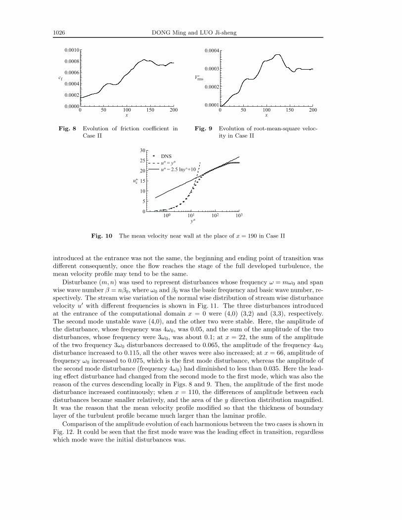
The evolution of wall friction coefficient and root-mean-square of perturbation velocity inCase II is shown in Figs. 8 and 9, respectively. It exhibits that the value of both the wall frictioncoefficient and the root-mean-square of perturbation appears at some definite descent at theplace of x = 60, which is more different compared to Figs. 2 and 3. The reason is that the mainunstable wave introduced in Case II is the second mode; from Fig. 7 it can be seen that theunstable area of the second mode was diminishing and the unstable area of the first mode wasincreasing during the transition process. The local descent is at the point, where x = 60 wasthe result of the leading effect wave changing from the second mode to the first mode.

The characteristic of mean stream wise velocity near wall at x = 190 in Case II is shownin Fig. 10, where the flow had already reached a full developed turbulent status. It can beseen that the figure is very similar to Fig. 6, which means that although the initial disturbance

1026 DONG Ming and LUO Ji-sheng

0.0010

0.0008

0.0006

0.0004

0.0002

0.00000 50 100 150 200

x

cf

Fig. 8 Evolution of friction coefficient inCase II

0.0004

0.0003

0.0002

0.00010 50 100 150 200

x

V'rms

Fig. 9 Evolution of root-mean-square veloc-ity in Case II

30

25

20

15

10

5

0100 101 102 103

y+

u+c

DNSu+ = y+

u+ = 2.5 lny++10

Fig. 10 The mean velocity near wall at the place of x = 190 in Case II

introduced at the entrance was not the same, the beginning and ending point of transition wasdifferent consequently, once the flow reaches the stage of the full developed turbulence, themean velocity profile may tend to be the same.

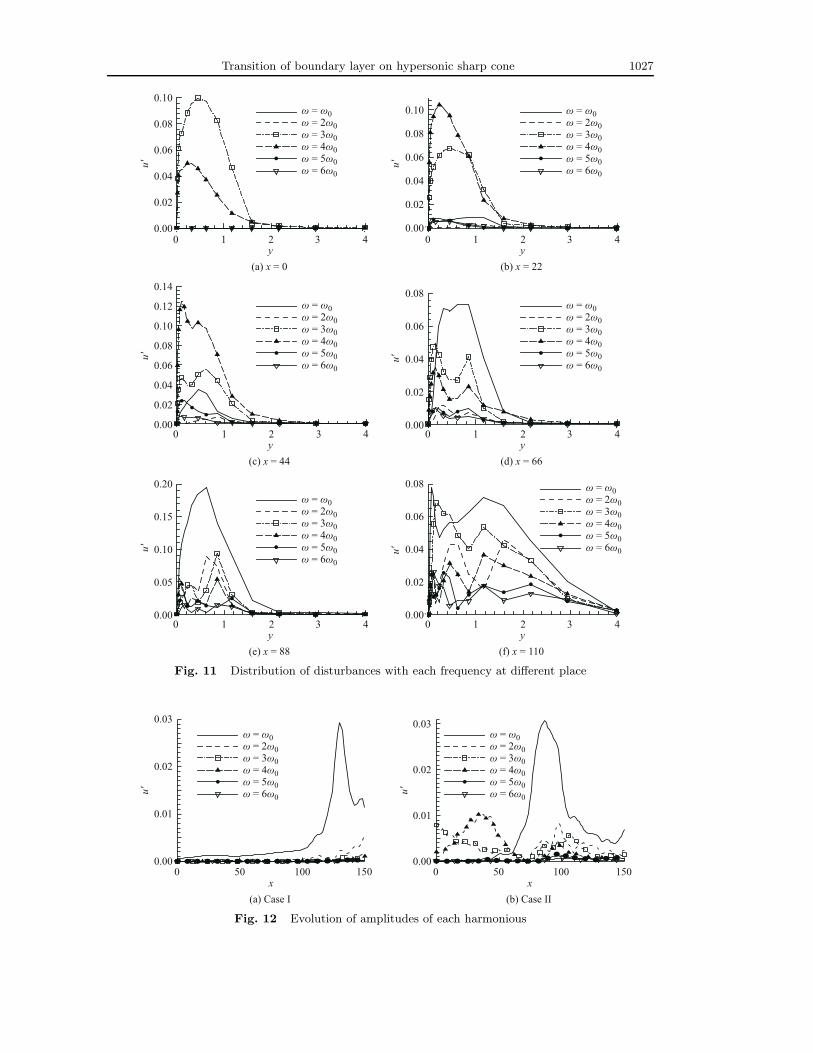
Disturbance (m, n) was used to represent disturbances whose frequency ω = mω0 and spanwise wave number β = nβ0, where ω0 and β0 was the basic frequency and basic wave number, re-spectively. The stream wise variation of the normal wise distribution of stream wise disturbancevelocity u′ with different frequencies is shown in Fig. 11. The three disturbances introducedat the entrance of the computational domain x = 0 were (4,0) (3,2) and (3,3), respectively.The second mode unstable wave (4,0), and the other two were stable. Here, the amplitude ofthe disturbance, whose frequency was 4ω0, was 0.05, and the sum of the amplitude of the twodisturbances, whose frequency were 3ω0, was about 0.1; at x = 22, the sum of the amplitudeof the two frequency 3ω0 disturbances decreased to 0.065, the amplitude of the frequency 4ω0

disturbance increased to 0.115, all the other waves were also increased; at x = 66, amplitude offrequency ω0 increased to 0.075, which is the first mode disturbance, whereas the amplitude ofthe second mode disturbance (frequency 4ω0) had diminished to less than 0.035. Here the lead-ing effect disturbance had changed from the second mode to the first mode, which was also thereason of the curves descending locally in Figs. 8 and 9. Then, the amplitude of the first modedisturbance increased continuously; when x = 110, the differences of amplitude between eachdisturbances became smaller relatively, and the area of the y direction distribution magnified.It was the reason that the mean velocity profile modified so that the thickness of boundarylayer of the turbulent profile became much larger than the laminar profile.

Comparison of the amplitude evolution of each harmonious between the two cases is shown inFig. 12. It could be seen that the first mode wave was the leading effect in transition, regardlesswhich mode wave the initial disturbances was.

Transition of boundary layer on hypersonic sharp cone 1027

0.10

0.08

0.06

0.04

0.02

0.000 1 2 3 4

y(a) x = 0

u' u'

u' u'

u' u'

0.10

0.08

0.06

0.04

0.02

0.000 1 2 3 4

y(b) x = 22

0.14

0.12

0.10

0.08

0.06

0.04

0.02

0.000 1 2 3 4

y(c) x = 44

0.08

0.06

0.04

0.02

0.000 1 2 3 4

y(d) x = 66

0.20

0.15

0.10

0.05

0.000 1 2 3 4

y(e) x = 88

0.08

0.06

0.04

0.02

0.000 1 2 3 4

y(f) x = 110

ω = ω0ω = 2ω0ω = 3ω0ω = 4ω0ω = 5ω0ω = 6ω0

ω = ω0ω = 2ω0ω = 3ω0ω = 4ω0ω = 5ω0ω = 6ω0

ω = ω0ω = 2ω0ω = 3ω0ω = 4ω0ω = 5ω0ω = 6ω0

ω = ω0ω = 2ω0ω = 3ω0ω = 4ω0ω = 5ω0ω = 6ω0

ω = ω0ω = 2ω0ω = 3ω0ω = 4ω0ω = 5ω0ω = 6ω0

ω = ω0ω = 2ω0ω = 3ω0ω = 4ω0ω = 5ω0ω = 6ω0

Fig. 11 Distribution of disturbances with each frequency at different place

0.03

0.02

0.01

0.000 50 100 150

x(a) Case I

u' u'

0.03

0.02

0.01

0.000 50 100 150

x(b) Case II

ω = ω0ω = 2ω0ω = 3ω0ω = 4ω0ω = 5ω0ω = 6ω0

ω = ω0ω = 2ω0ω = 3ω0ω = 4ω0ω = 5ω0ω = 6ω0

Fig. 12 Evolution of amplitudes of each harmonious

1028 DONG Ming and LUO Ji-sheng

3 Conclusions

Being different from flat boundary layer, the sharp cone boundary layer has span wise curva-ture which varies along stream wise; however, the numerical study on a hypersonic compressiblesharp cone boundary layer with zero angle of attack, oncoming Mach number 6, drew similarconclusions: transition is not only the process of the high-order harmonious generation and itincreases because of nonlinear effect essentially; in this process, the rapid change of stability ofthe mean flow profile makes great effect. These variations determined which waves would in-crease, and which would decrease. Being similar to the flat boundary layer, the rapid variationof stability of averaging flow profile made the first mode waves increase rapidly, and the secondmode waves decrease gradually. That was to say, the first mode unstable wave was the leadingeffect in transition, regardless of which mode wave the initial disturbance introduced was. And,no matter what initial disturbances occurred, once the turbulence appeared, the mean velocityprofile may tend to the same.

References

[1] Dong Ming, Luo Jisheng, Cao Wei. Numerical investigation of evolution of disturbances in super-sonic sharp cone boundary layer[J]. Applied Mathematics and Mechanics (English Edition), 2006,27(6):713–719.

[2] Luo Jisheng, Wang Xinjun, Zhou Heng. Inherent mechanism of breakdown in laminar-turbulenttransition of plane channel flows[J]. Science in China, Ser G, Physics, Mechanics and Astronomy,2005, 48(2):228–236.

[3] Huang Zhangfeng, Cao Wei, Zhou Heng. The mechanism of breakdown in laminar-turbulent tran-sition of a supersonic boundary layer on a flat plate-temporal mode[J]. Science in China, Ser G,Physics, Mechanics and Astronomy, 2005, 48(5):614–625.

[4] Cao Wei, Huang Zhangfeng, Zhou Heng. Study of mechanism of breakdown in laminar-turbulenttransition of supersonic boundary layer on flat plate[J]. Applied Mathematics and Mechanics(English Edition), 2006, 27(4):425–434.

[5] Tong Binggang, Kong Xiangyan, Deng Guohua. Dynamics of gas flow[M]. Beijing: Higher Edu-cation Press, 1989, 140–142 (in Chinese).

[6] Zhao Gengfu. Laminar flow control of supersonic/ hypersonic three-dimensional boundary layer[J].Chinese Journal of Theoretical and Applied Mechanics, 2001, 33(4):519–524 (in Chinese).

[7] Zhang Dongming, Luo Jisheng, Zhou Heng. A mechanism for excitation of coherent structuresin wall region of a turbulent boundary layer[J]. Applied Mathematics and Mechanics (EnglishEdition), 2005, 26(4):415–422.