Embed Size (px)
Citation preview
1 OCTOBER 2000 3219E S H E L A N D F A R R E L L
q 2000 American Meteorological Society
Mechanisms of Eastern Mediterranean Rainfall Variability
GIDON ESHEL
Department of the Geophysical Sciences, The University of Chicago, Chicago, Illinois
BRIAN F. FARRELL
Department of Earth and Planetary Sciences, Harvard University, Cambridge, Massachusetts
(Manuscript received 23 November 1998, in final form 20 January 2000)
ABSTRACT
This paper presents a simple theory for the association between observed eastern Mediterranean (EM) rainfallanomalies and North Atlantic (NA) climate variability. Large-scale NA atmospheric mass rearrangements, pri-marily a modulation of the Icelandic low and the subtropical high pressure systems, tend to extend beyond theNA. A particularly strong such teleconnection exists between the northern NA and southern Europe and theMediterranean Basin. Pressure anomalies over Greenland–Iceland are thus associated with reversed-polarityanomalies centered over the northern Adriatic, affecting the entire Mediterranean Basin; elevated Greenlandpressure is accompanied by an anomalous cyclone over the Mediterranean, and a Mediterranean high pressuresystem is present when pressure over Greenland is reduced. In the EM, these anomalies result in anomaloussoutherlies during Greenland highs, and northerlies during Greenland lows. Eastern Mediterranean southerlieswarm the EM, while northerlies cool locally. Because heat advection by horizontal and vertical motions dominatethe EM thermodynamic equation (or, put differently, because thickness advection dominates the omega equation),cooling by northerly winds results in enhanced subsidence. Conversely, warming by anomalous EM southerliesproduces enhanced ascent. These vertical motion anomalies modify the stability of the mean column, resultingin the observed EM rainfall anomalies.
1. Introduction
In recent years, considerable attention has been de-voted to climate variability outside the deep Tropics.Common to many of the mechanisms advanced by var-ious authors to explain the variability are large-scalestationary wave anomalies (Battisti et al. 1995; Blade1997; Frankignoul 1985; Kushnir and Wallace 1989;Kushnir 1994; Latif and Barnett 1994, 1996; Molteniand Palmer 1993; Venzke et al. 1998; Wallace et al.1990, 1992; Weng and Neelin 1998, among others). Adiscussion of stationary wave variability over the NorthAtlantic (NA) sector can be found in any of the abovereferences. The basic structure of the variability is afairly simple modulation of the relative intensity of theclimatological subtropical high and subpolar low—theNA oscillation (NAO; e.g., Hurrell 1995; Kushnir 1994,1999; McCartney 1997; Rodwell et al. 1999). This mod-ification of the NA mean meridional pressure gradientand the associated thermal wind balance of the midlat-
Corresponding author address: Dr. Gidon Eshel, Dept. of the Geo-physical Sciences, The University of Chicago, 5734 S. Ellis Ave.,Chicago, IL 60637.E-mail: [email protected]
itude westerlies affects the intensity and spatial detailsof the westerlies, and thus downstream climates. Es-pecially relevant to the current study, Hurrell (1995)and Hurrell and van Loon (1997) have demonstrated theimportance of the NAO to regional patterns of temper-ature and water vapor advection. Because anomalies as-sociated with the NAO (and other extratropical station-ary wave phenomena such as the Pacific–North Americapattern) are typically centered over the ocean, they affecthuman populations primarily through their remote in-fluences. These remote impacts have enjoyed less at-tention than the anomalies themselves, and their de-scription and dynamical understanding are incomplete(Hurrell and van Loon 1997; Steinberger and Gazit-Yaari 1996). Here we explore a specific example ofremote effects of stationary wave anomalies, namely,eastern Mediterranean (EM) climate anomalies associ-ated with NA anomalies. While there is no reason toassume this example is physically unique, its societalimpact is substantial. Dry summers (Rodwell and Hos-kins 1996) render winter rainfall the sole, and highlycapricious, source of renewable water in the EM. Asmost economies around the EM are still developing,they depend heavily on water, and are very susceptibleto droughts. Thus both fundamental climatic processes
3220 VOLUME 57J O U R N A L O F T H E A T M O S P H E R I C S C I E N C E S
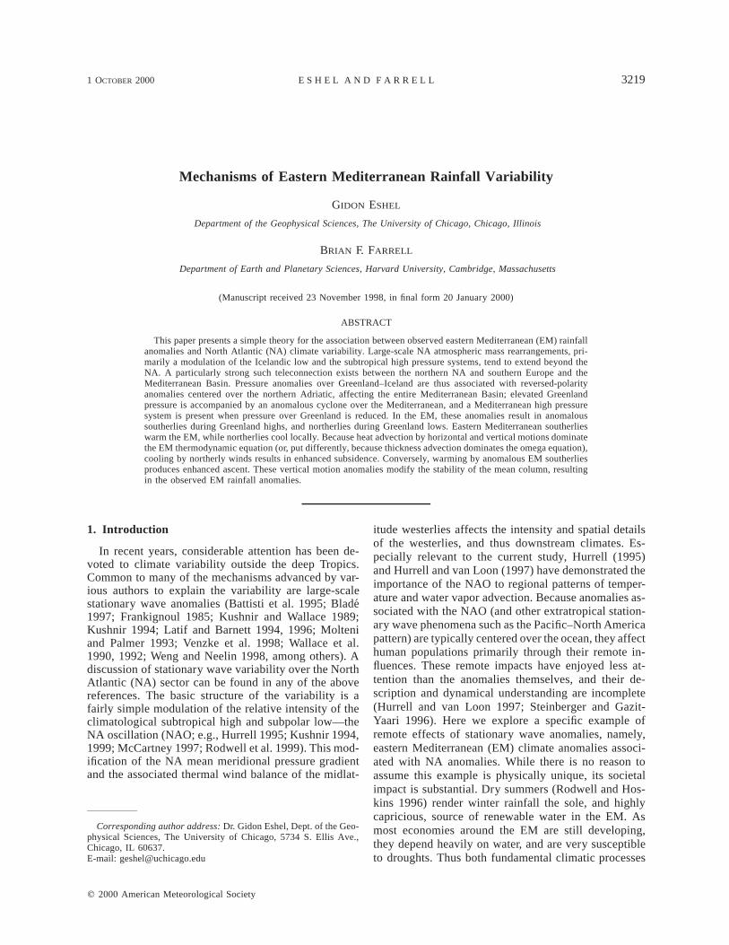
FIG. 1. Schematic of the NA–EM teleconnection. Eastern Mediterranean pressure anomalies are part oflarge-scale anomalies over the NA–Europe–Mediterranean sector. The Mediterranean experiences high (low)pressure anomalies during low (high) EM rainfall anomalies. This yields northeasterlies during times oflow rainfall, and southwesterlies during high EM rainfall, shown by the thick arrows. During EM droughts,this anomalous wind cools the EM. The cooling is partly compensated by enhanced subsidence, whichresults in increased lower tropospheric static stability and suppressed precipitation. In times of high EMrainfall (lower panel), these processes are reversed.
and their socioeconomical consequences are manifestedin the EM, and provide the motivation for this paper.
To enhance readability, we summarize in advance themain ideas of the paper here and in Fig. 1. We arguethat EM rainfall variability is caused by subsidenceanomalies associated with the NA. Variability of tro-pospheric mass distribution over the NA–Mediterraneansector assumes the form of a seasonally stationary wavepattern with opposite-sign nodes over Greenland–Ice-land and the northern Mediterranean. Thus when Green-land’s pressure is anomalously high, an anomalous lowcovers the Mediterranean and southern Europe, yieldingEM southerlies; when Greenland pressure is anoma-lously low, EM northerlies prevail. These wind anom-alies are strong and persistent, and significantly alterpatterns of heat advection. The ensuing imbalance be-tween the mass and motion fields is followed by dy-namic adjustment. The adjustment process modifies sub-sidence intensity, strongly affecting rainfall. Enhancedsubsidence and reduced EM rainfall accompany cooling
by northerly winds characteristic of a Greenland low.Conversely, warming by southerly winds during Green-land highs results in weakened subsidence and inten-sified EM precipitation.
2. Data and analysis
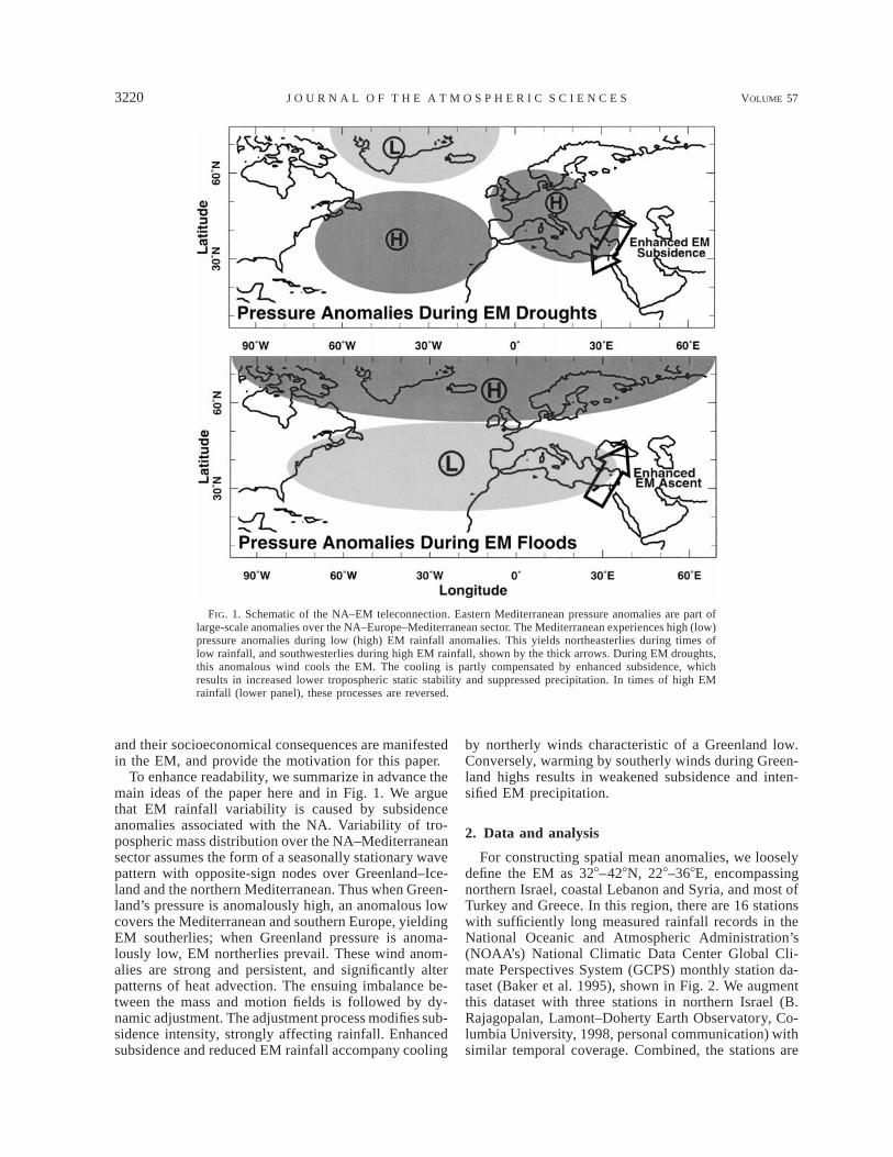
For constructing spatial mean anomalies, we looselydefine the EM as 328–428N, 228–368E, encompassingnorthern Israel, coastal Lebanon and Syria, and most ofTurkey and Greece. In this region, there are 16 stationswith sufficiently long measured rainfall records in theNational Oceanic and Atmospheric Administration’s(NOAA’s) National Climatic Data Center Global Cli-mate Perspectives System (GCPS) monthly station da-taset (Baker et al. 1995), shown in Fig. 2. We augmentthis dataset with three stations in northern Israel (B.Rajagopalan, Lamont–Doherty Earth Observatory, Co-lumbia University, 1998, personal communication) withsimilar temporal coverage. Combined, the stations are
1 OCTOBER 2000 3221E S H E L A N D F A R R E L L
FIG. 2. Rain gauge station distribution, from the ungridded data of Baker et al. (1994). Symbols denote temporalcoverage, as indicated by the legend.
distributed throughout the EM (thus sampling it rea-sonably well) and span a wide range of geographicalsettings and elevations. The resultant record is shownin Fig. 3b. It is discontinuous in 1985 as some stationrecords end at that year and are replaced by recordsfrom nearby other stations, as indicated on Fig. 2. Agood agreement between the records derived from thetwo station sets during 1980–85 (not shown) suggeststhat the effect of the change is minor.
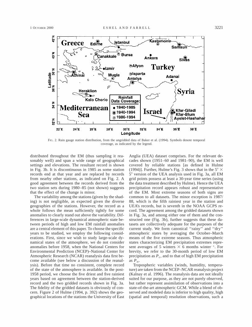
The variability among the stations (given by the shad-ing) is not negligible, as expected given the diversegeographies of the stations. However, the record as awhole follows the mean sufficiently tightly for someanomalies to clearly stand out above the variability. Dif-ferences in large-scale dynamical atmospheric state be-tween periods of high and low EM rainfall anomaliesare a central element of this paper. To choose the specificyears to be studied, we employ the following consid-erations. First, since we wish to study large-scale dy-namical states of the atmosphere, we do not consideranomalies before 1958, when the National Centers forEnvironmental Prediction (NCEP)–National Center forAtmospheric Research (NCAR) reanalysis data first be-come available (see below a discussion of the reanal-ysis). Before that time no consistent, complete recordof the state of the atmosphere is available. In the post-1958 period, we choose the five driest and five rainiestyears based on agreement between the station-derivedrecord and the two gridded records shown in Fig. 3a.The fidelity of the gridded datasets is obviously of con-cern. Figure 2 of Hulme (1994, p. 392) shows the geo-graphical locations of the stations the University of East
Anglia (UEA) dataset comprises. For the relevant de-cades shown (1951–60 and 1981–90), the EM is wellcovered by reliable stations [as defined in Hulme(1994)]. Further, Hulme’s Fig. 3 shows that in the 58 358 version of the UEA analysis used in Fig. 3a, all EMgrid points possess at least a 30-year time series (usingthe data treatment described by Hulme). Hence the UEAprecipitation record appears robust and representativeof the EM. Most extreme seasons of both signs arecommon to all datasets. The minor exception is 1987/88, which is the fifth rainiest year in the station andUEA’s records, but is seventh in the NOAA GCPS re-cord. The agreement among the gridded datasets shownin Fig. 3a, and among either one of them and the con-structed one (Fig. 3b), further suggests that these da-tasets are collectively adequate for the purposes of thecurrent study. We form canonical ‘‘rainy’’ and ‘‘dry’’atmospheric states by averaging the October–Marchmeans of the five extreme seasons. Thus atmosphericstates characterizing EM precipitation extremes repre-sent averages of 5 winters 3 6 months winter21. Forbrevity, we refer to the 30-month period of low EMprecipitation as PL, and to that of high EM precipitationas PH.
Tropospheric variables (winds, humidity, tempera-ture) are taken from the NCEP–NCAR reanalysis project(Kalnay et al. 1996). The reanalysis data are not ideallysuited for our purpose, as they are not purely observed,but rather represent assimilation of observations into astate-of-the-art atmospheric GCM. While a blend of ob-served and modeled data is inferior to high quality, high(spatial and temporal) resolution observations, such a
3222 VOLUME 57J O U R N A L O F T H E A T M O S P H E R I C S C I E N C E S
FIG. 3. Records of EM winter rainfall anomalies. (a) Two observational records of gridded pre-cipitation anomalies; thick line, NOAA’s NCDC GCPS (Baker et al. 1994); thin line, UEA/CRU(Hulme 1992, 1994). (b) Mean (thick solid line) and standard deviation (shaded region) of the stationdata shown in Fig. 1. The gap distinguishes the two data-coverage periods indicated on Fig. 1. Thefive rainiest and driest winters are denoted by small dashes originating from the corresponding datapoints up or down, respectively. The thin line is the mean (thick curve), convolved with [1, 2, 3, 2,1]/9, i.e., a 5-yr weighted running mean.
dataset does not currently exist, and there is not enoughstation data to calculate dynamical fields (such as di-vergence) accurately. On the other hand, the model’sthermodynamics are strongly constrained by data indata-dense regions such as the Mediterranean. For ex-ample, Trenberth and Guillemot (1998, their Fig. 3) pre-sent a global correlation map spanning 60 months oftotal-column precipitable water in the NCEP–NCAR re-analysis data versus remotely sensed observations[NASA Water Vapor Project (NVAP)]. Correlations ex-ceed 0.90 throughout the NA, Mediterranean, and Eu-rope, but drop somewhat to the south of the region ofinterest, toward the central Red Sea and the Sahara.Hence the dynamically consistent assimilated fields,while clearly imperfect, are the best currently availableapproximation to the true fields. Transient errors areaveraged out in the monthly mean data we use, and arefurther reduced by the 30-month averaging describedabove. Similarly, the characteristic space scales for theanomalies analyzed here are fairly large [typically O(103 10 grid points)], and are thus relatively immune tosmall-scale noise in the assimilation model. Our resultsshould therefore be considered tentative, awaiting future
improvements of the observational network. With theexception of rainfall and surface wind stress [calculatedfrom ship wind estimates (daSilva et al. 1994)], data arefrom the reanalysis project.
Significance tests
We present significance levels of both anomalies aand correlations r, employing the t test. To form t sta-tistics, we use t 5 r[(df 2 2)/(1 2 r2)]1/2 and t 5 (a2 a)/ (Philips 1982), where a and are a’s temporalt ts sa a
mean and standard error. In estimating the number ofdegrees of freedom df, we make the rather stringentassumption that the decorrelation timescale ;2 yr (i.e.,that only every 2-yr period represents an independentrealization; df 5 N/2, where N is the time series lengthin years). [Typical gridpoint autocorrelation functionsof used anomaly fields indicate that actual characteristictemporal decorrelation scales are typically less (oftenmuch less) than 10 months on average. Hence, the as-sumption of a 2-yr decorrelation timescale represents aconservative upper bound.] To exclude spurious cor-relations primarily due to trends in the data, all reported
1 OCTOBER 2000 3223E S H E L A N D F A R R E L L
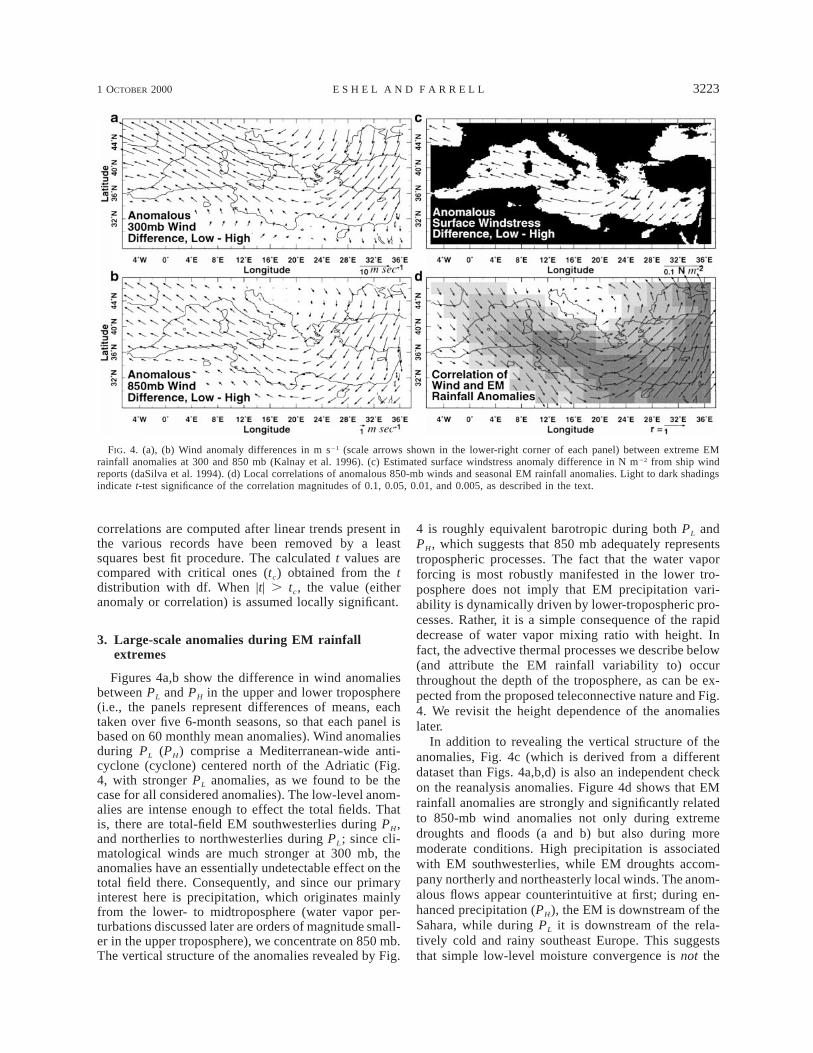
FIG. 4. (a), (b) Wind anomaly differences in m s21 (scale arrows shown in the lower-right corner of each panel) between extreme EMrainfall anomalies at 300 and 850 mb (Kalnay et al. 1996). (c) Estimated surface windstress anomaly difference in N m22 from ship windreports (daSilva et al. 1994). (d) Local correlations of anomalous 850-mb winds and seasonal EM rainfall anomalies. Light to dark shadingsindicate t-test significance of the correlation magnitudes of 0.1, 0.05, 0.01, and 0.005, as described in the text.
correlations are computed after linear trends present inthe various records have been removed by a leastsquares best fit procedure. The calculated t values arecompared with critical ones (tc) obtained from the tdistribution with df. When |t| . tc, the value (eitheranomaly or correlation) is assumed locally significant.
3. Large-scale anomalies during EM rainfallextremes
Figures 4a,b show the difference in wind anomaliesbetween PL and PH in the upper and lower troposphere(i.e., the panels represent differences of means, eachtaken over five 6-month seasons, so that each panel isbased on 60 monthly mean anomalies). Wind anomaliesduring PL (PH) comprise a Mediterranean-wide anti-cyclone (cyclone) centered north of the Adriatic (Fig.4, with stronger PL anomalies, as we found to be thecase for all considered anomalies). The low-level anom-alies are intense enough to effect the total fields. Thatis, there are total-field EM southwesterlies during PH,and northerlies to northwesterlies during PL; since cli-matological winds are much stronger at 300 mb, theanomalies have an essentially undetectable effect on thetotal field there. Consequently, and since our primaryinterest here is precipitation, which originates mainlyfrom the lower- to midtroposphere (water vapor per-turbations discussed later are orders of magnitude small-er in the upper troposphere), we concentrate on 850 mb.The vertical structure of the anomalies revealed by Fig.
4 is roughly equivalent barotropic during both PL andPH, which suggests that 850 mb adequately representstropospheric processes. The fact that the water vaporforcing is most robustly manifested in the lower tro-posphere does not imply that EM precipitation vari-ability is dynamically driven by lower-tropospheric pro-cesses. Rather, it is a simple consequence of the rapiddecrease of water vapor mixing ratio with height. Infact, the advective thermal processes we describe below(and attribute the EM rainfall variability to) occurthroughout the depth of the troposphere, as can be ex-pected from the proposed teleconnective nature and Fig.4. We revisit the height dependence of the anomalieslater.
In addition to revealing the vertical structure of theanomalies, Fig. 4c (which is derived from a differentdataset than Figs. 4a,b,d) is also an independent checkon the reanalysis anomalies. Figure 4d shows that EMrainfall anomalies are strongly and significantly relatedto 850-mb wind anomalies not only during extremedroughts and floods (a and b) but also during moremoderate conditions. High precipitation is associatedwith EM southwesterlies, while EM droughts accom-pany northerly and northeasterly local winds. The anom-alous flows appear counterintuitive at first; during en-hanced precipitation (PH), the EM is downstream of theSahara, while during PL it is downstream of the rela-tively cold and rainy southeast Europe. This suggeststhat simple low-level moisture convergence is not the
3224 VOLUME 57J O U R N A L O F T H E A T M O S P H E R I C S C I E N C E S
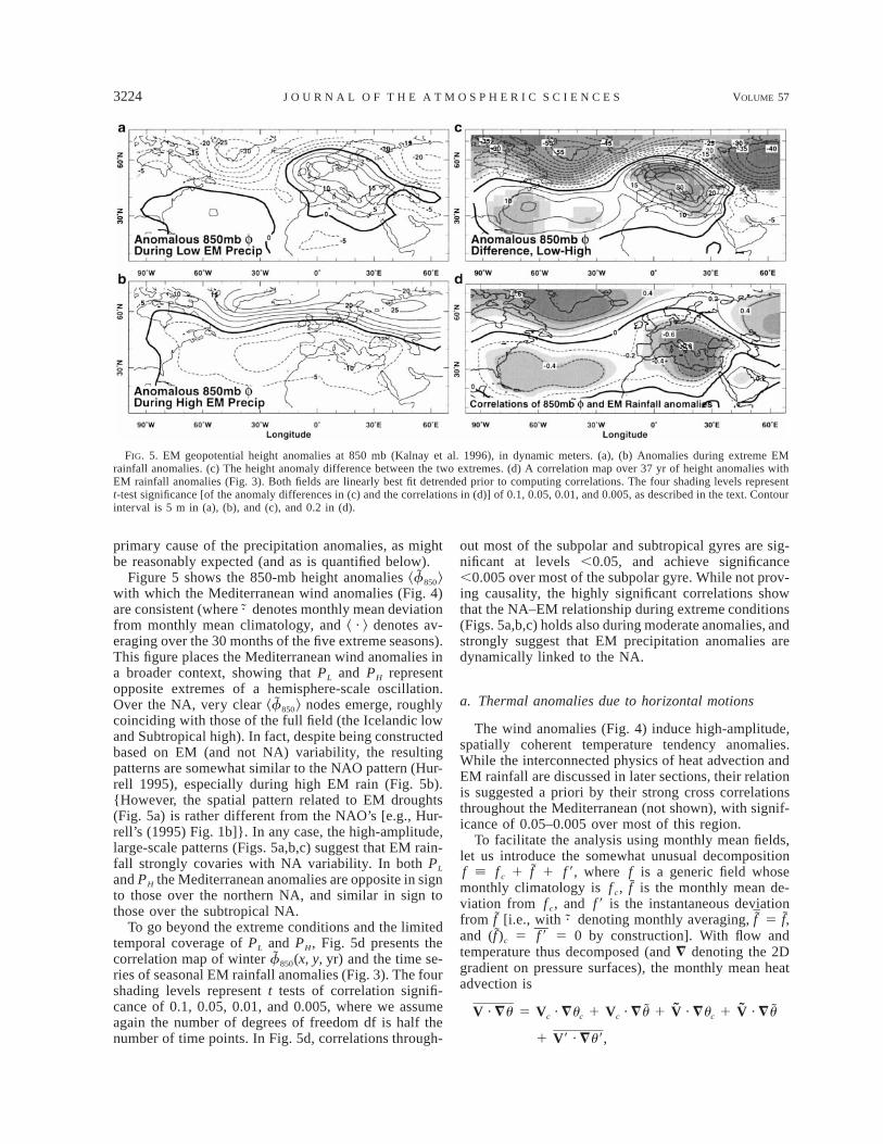
FIG. 5. EM geopotential height anomalies at 850 mb (Kalnay et al. 1996), in dynamic meters. (a), (b) Anomalies during extreme EMrainfall anomalies. (c) The height anomaly difference between the two extremes. (d) A correlation map over 37 yr of height anomalies withEM rainfall anomalies (Fig. 3). Both fields are linearly best fit detrended prior to computing correlations. The four shading levels representt-test significance [of the anomaly differences in (c) and the correlations in (d)] of 0.1, 0.05, 0.01, and 0.005, as described in the text. Contourinterval is 5 m in (a), (b), and (c), and 0.2 in (d).
primary cause of the precipitation anomalies, as mightbe reasonably expected (and as is quantified below).
Figure 5 shows the 850-mb height anomalies ^ &f850
with which the Mediterranean wind anomalies (Fig. 4)are consistent (where denotes monthly mean deviation·from monthly mean climatology, and ^ · & denotes av-eraging over the 30 months of the five extreme seasons).This figure places the Mediterranean wind anomalies ina broader context, showing that PL and PH representopposite extremes of a hemisphere-scale oscillation.Over the NA, very clear ^ & nodes emerge, roughlyf850
coinciding with those of the full field (the Icelandic lowand Subtropical high). In fact, despite being constructedbased on EM (and not NA) variability, the resultingpatterns are somewhat similar to the NAO pattern (Hur-rell 1995), especially during high EM rain (Fig. 5b).{However, the spatial pattern related to EM droughts(Fig. 5a) is rather different from the NAO’s [e.g., Hur-rell’s (1995) Fig. 1b]}. In any case, the high-amplitude,large-scale patterns (Figs. 5a,b,c) suggest that EM rain-fall strongly covaries with NA variability. In both PL
and PH the Mediterranean anomalies are opposite in signto those over the northern NA, and similar in sign tothose over the subtropical NA.
To go beyond the extreme conditions and the limitedtemporal coverage of PL and PH, Fig. 5d presents thecorrelation map of winter and the time se-f (x, y, yr)850
ries of seasonal EM rainfall anomalies (Fig. 3). The fourshading levels represent t tests of correlation signifi-cance of 0.1, 0.05, 0.01, and 0.005, where we assumeagain the number of degrees of freedom df is half thenumber of time points. In Fig. 5d, correlations through-
out most of the subpolar and subtropical gyres are sig-nificant at levels ,0.05, and achieve significance,0.005 over most of the subpolar gyre. While not prov-ing causality, the highly significant correlations showthat the NA–EM relationship during extreme conditions(Figs. 5a,b,c) holds also during moderate anomalies, andstrongly suggest that EM precipitation anomalies aredynamically linked to the NA.
a. Thermal anomalies due to horizontal motions
The wind anomalies (Fig. 4) induce high-amplitude,spatially coherent temperature tendency anomalies.While the interconnected physics of heat advection andEM rainfall are discussed in later sections, their relationis suggested a priori by their strong cross correlationsthroughout the Mediterranean (not shown), with signif-icance of 0.05–0.005 over most of this region.
To facilitate the analysis using monthly mean fields,let us introduce the somewhat unusual decompositionf [ f c 1 f 1 f 9, where f is a generic field whosemonthly climatology is f c, f is the monthly mean de-viation from f c, and f 9 is the instantaneous deviationfrom [i.e., with denoting monthly averaging, 5 f,f · fand 5 f 9 5 0 by construction]. With flow and(f )c
temperature thus decomposed (and = denoting the 2Dgradient on pressure surfaces), the monthly mean heatadvection is
˜ ˜V · =u 5 V · =u 1 V · =u 1 V · =u 1 V · =uc c c c
1 V9 · =u9,
1 OCTOBER 2000 3225E S H E L A N D F A R R E L L
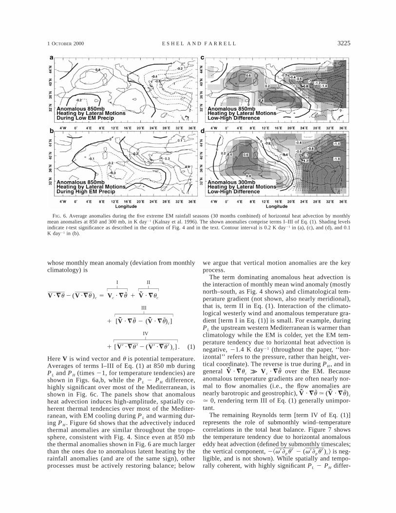
FIG. 6. Average anomalies during the five extreme EM rainfall seasons (30 months combined) of horizontal heat advection by monthlymean anomalies at 850 and 300 mb, in K day21 (Kalnay et al. 1996). The shown anomalies comprise terms I–III of Eq. (1). Shading levelsindicate t-test significance as described in the caption of Fig. 4 and in the text. Contour interval is 0.2 K day21 in (a), (c), and (d), and 0.1K day21 in (b).
whose monthly mean anomaly (deviation from monthlyclimatology) is
I IIz z]}}} ]}}}| | | |
˜V · =u 2 (V · =u ) 5 V · =u 1 V · =uc c c
IIIz}}}}}}}}}}| |
˜ ˜1 [V · =u 2 (V · =u) ]c
IVz}}}}}}}}}}}| |
1 [V9 · =u9 2 (V9 · =u9) ] . (1)c
Here V is wind vector and u is potential temperature.Averages of terms I–III of Eq. (1) at 850 mb duringPL and PH (times 21, for temperature tendencies) areshown in Figs. 6a,b, while the PL 2 PH difference,highly significant over most of the Mediterranean, isshown in Fig. 6c. The panels show that anomalousheat advection induces high-amplitude, spatially co-herent thermal tendencies over most of the Mediter-ranean, with EM cooling during PL and warming dur-ing PH . Figure 6d shows that the advectively inducedthermal anomalies are similar throughout the tropo-sphere, consistent with Fig. 4. Since even at 850 mbthe thermal anomalies shown in Fig. 6 are much largerthan the ones due to anomalous latent heating by therainfall anomalies (and are of the same sign), otherprocesses must be actively restoring balance; below
we argue that vertical motion anomalies are the keyprocess.
The term dominating anomalous heat advection isthe interaction of monthly mean wind anomaly (mostlynorth–south, as Fig. 4 shows) and climatological tem-perature gradient (not shown, also nearly meridional),that is, term II in Eq. (1). Interaction of the climato-logical westerly wind and anomalous temperature gra-dient [term I in Eq. (1)] is small. For example, duringPL the upstream western Mediterranean is warmer thanclimatology while the EM is colder, yet the EM tem-perature tendency due to horizontal heat advection isnegative, 21.4 K day21 (throughout the paper, ‘‘hor-izontal’’ refers to the pressure, rather than height, ver-tical coordinate). The reverse is true during PH , and ingeneral V · =uc k Vc · = over the EM. Becauseuanomalous temperature gradients are often nearly nor-mal to flow anomalies (i.e., the flow anomalies arenearly barotropic and geostrophic), V · = . (V · = )cu u. 0, rendering term III of Eq. (1) generally unimpor-tant.
The remaining Reynolds term [term IV of Eq. (1)]represents the role of submonthly wind–temperaturecorrelations in the total heat balance. Figure 7 showsthe temperature tendency due to horizontal anomalouseddy heat advection (defined by submonthly timescales;the vertical component, 2^v9]pu9 2 (v9]pu9)c& is neg-ligible, and is not shown). While spatially and tempo-rally coherent, with highly significant PL 2 PH differ-
3226 VOLUME 57J O U R N A L O F T H E A T M O S P H E R I C S C I E N C E S
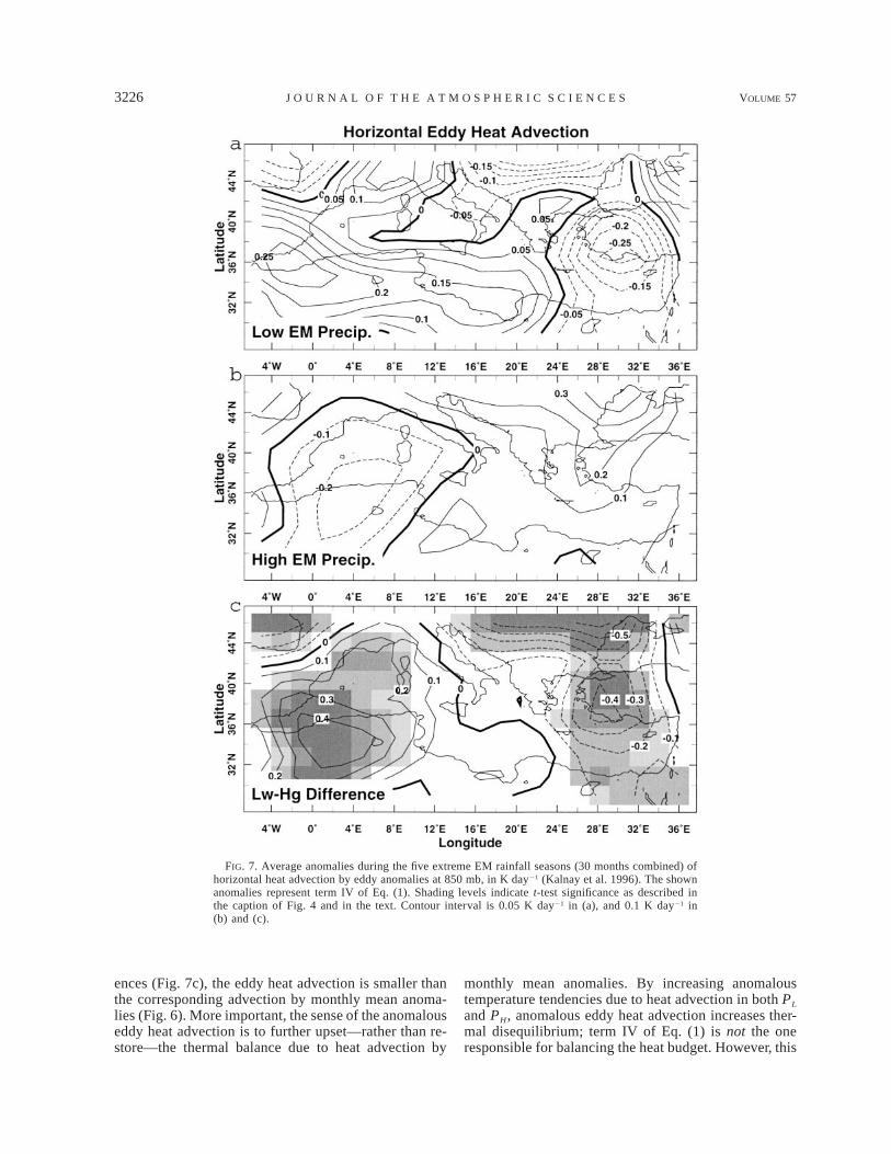
FIG. 7. Average anomalies during the five extreme EM rainfall seasons (30 months combined) ofhorizontal heat advection by eddy anomalies at 850 mb, in K day21 (Kalnay et al. 1996). The shownanomalies represent term IV of Eq. (1). Shading levels indicate t-test significance as described inthe caption of Fig. 4 and in the text. Contour interval is 0.05 K day21 in (a), and 0.1 K day21 in(b) and (c).
ences (Fig. 7c), the eddy heat advection is smaller thanthe corresponding advection by monthly mean anoma-lies (Fig. 6). More important, the sense of the anomalouseddy heat advection is to further upset—rather than re-store—the thermal balance due to heat advection by
monthly mean anomalies. By increasing anomaloustemperature tendencies due to heat advection in both PL
and PH, anomalous eddy heat advection increases ther-mal disequilibrium; term IV of Eq. (1) is not the oneresponsible for balancing the heat budget. However, this
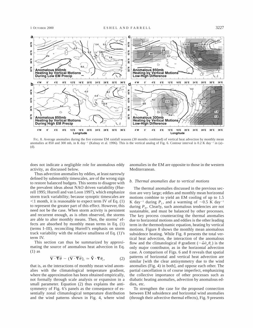
1 OCTOBER 2000 3227E S H E L A N D F A R R E L L
FIG. 8. Average anomalies during the five extreme EM rainfall seasons (30 months combined) of vertical heat advection by monthly meananomalies at 850 and 300 mb, in K day21 (Kalnay et al. 1996). This is the vertical analog of Fig. 6. Contour interval is 0.2 K day21 in (a)–(d).
does not indicate a negligible role for anomalous eddyactivity, as discussed below.
Thus advection anomalies by eddies, at least narrowlydefined by submonthly timescales, are of the wrong signto restore balanced budgets. This seems to disagree withthe prevalent ideas about NAO driven variability (Hur-rell 1995; Hurrell and van Loon 1997), which emphasizestorm track variability; because synoptic timescales are,1 month, it is reasonable to expect term IV of Eq. (1)to represent the greater part of this effect. However, thisneed not be the case. When storm activity is persistentand recurrent enough, as is often observed, the stormsare able to alter monthly means. Then, the storms’ ef-fects are absorbed by monthly mean terms in Eq. (1)(terms I–III), reconciling Hurrell’s emphasis on stormtrack variability with the relative smallness of Eq. (1)’sterm IV.
This section can thus be summarized by approxi-mating the source of anomalous heat advection in Eq.(1) as
˜V · =u 2 (V · =u ) . V · =u , (2)c c
that is, as the interactions of monthly mean wind anom-alies with the climatological temperature gradient,where the approximation has been obtained empirically,not formally through scale analysis or expansion in asmall parameter. Equation (2) thus explains the anti-symmetry of Fig. 6’s panels as the consequence of es-sentially zonal climatological temperature distributionand the wind patterns shown in Fig. 4, where wind
anomalies in the EM are opposite to those in the westernMediterranean.
b. Thermal anomalies due to vertical motions
The thermal anomalies discussed in the previous sec-tion are very large; eddies and monthly mean horizontalmotions combine to yield an EM cooling of up to 1.5K day21 during PL, and a warming of ;0.5 K day21
during PH. Clearly, such anomalous tendencies are notsustainable, and must be balanced by other processes.The key process counteracting the thermal anomaliesdue to horizontal motions and eddies is the other leadingterm in the thermodynamic equation, heating by verticalmotions. Figure 8 shows the monthly mean anomaloussubsidence heating. While Fig. 8 presents the total ver-tical heat advection, the interaction of the anomalousflow and the climatological u gradient ( ) is the2v] up c
only major contributor, as in the horizontal advectioncase. A comparison of Figs. 6 and 8 reveals that spatialpatterns of horizontal and vertical heat advection aresimilar [with the clear antisymmetry due to the windanomalies (Fig. 4) in both], and oppose each other. Thepartial cancellation is of course imperfect, emphasizingthe collective importance of other processes such asdiabatic heating anomalies, advection by anomalous ed-dies, etc.
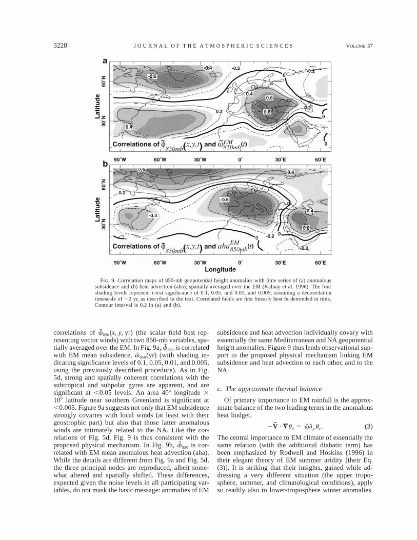
To strengthen the case for the proposed connectionbetween EM subsidence and horizontal wind anomalies(through their advective thermal effects), Fig. 9 presents
3228 VOLUME 57J O U R N A L O F T H E A T M O S P H E R I C S C I E N C E S
FIG. 9. Correlation maps of 850-mb geopotential height anomalies with time series of (a) anomaloussubsidence and (b) heat advection (aha), spatially averaged over the EM (Kalnay et al. 1996). The fourshading levels represent t-test significance of 0.1, 0.05, and 0.01, and 0.005, assuming a decorrelationtimescale of ;2 yr, as described in the text. Correlated fields are first linearly best fit detrended in time.Contour interval is 0.2 in (a) and (b).
correlations of (the scalar field best rep-f (x, y, yr)850
resenting vector winds) with two 850-mb variables, spa-tially averaged over the EM. In Fig. 9a, is correlatedf850
with EM mean subsidence, (with shading in-v (yr)850
dicating significance levels of 0.1, 0.05, 0.01, and 0.005,using the previously described procedure). As in Fig.5d, strong and spatially coherent correlations with thesubtropical and subpolar gyres are apparent, and aresignificant at ,0.05 levels. An area 408 longitude 3108 latitude near southern Greenland is significant at,0.005. Figure 9a suggests not only that EM subsidencestrongly covaries with local winds (at least with theirgeostrophic part) but also that those latter anomalouswinds are intimately related to the NA. Like the cor-relations of Fig. 5d, Fig. 9 is thus consistent with theproposed physical mechanism. In Fig. 9b, is cor-f850
related with EM mean anomalous heat advection (aha).While the details are different from Fig. 9a and Fig. 5d,the three principal nodes are reproduced, albeit some-what altered and spatially shifted. These differences,expected given the noise levels in all participating var-iables, do not mask the basic message: anomalies of EM
subsidence and heat advection individually covary withessentially the same Mediterranean and NA geopotentialheight anomalies. Figure 9 thus lends observational sup-port to the proposed physical mechanism linking EMsubsidence and heat advection to each other, and to theNA.
c. The approximate thermal balance
Of primary importance to EM rainfall is the approx-imate balance of the two leading terms in the anomalousheat budget,
2V · =uc . ]puc.v (3)
The central importance to EM climate of essentially thesame relation (with the additional diabatic term) hasbeen emphasized by Rodwell and Hoskins (1996) intheir elegant theory of EM summer aridity [their Eq.(3)]. It is striking that their insights, gained while ad-dressing a very different situation (the upper tropo-sphere, summer, and climatological conditions), applyso readily also to lower-troposphere winter anomalies.
1 OCTOBER 2000 3229E S H E L A N D F A R R E L L
Equation (3) suggests that the subsidence anomalies(essentially Fig. 8 rescaled) and the horizontal advectivethermal anomalies are dynamically mutually consistent,satisfying
. 2(V · =uc)(]puc)21.v (4)
The validity of Eqs. (3) and (4) is corroborated by thefact that individual gridpoint correlations between andv(V · =u) 2 (V · =u)c are between 20.5 and 20.7 (sig-nificant at ,0.05) over most of the Mediterranean. Fur-ther, the correlations reach significance ,0.01 over asizable area covering northwest Italy, southeast France,and the Gulf of Lions. Most important, the correlationsover the entire EM reach values ,20.8 (significance, 0.005).
Combined, the anomalous horizontal winds (Fig. 4),their thermal consequences (Figs. 6 and 8), and thevertical motions implied by Eq. (4) provide a concisedescription of the mechanism underlying the EM pre-cipitation anomalies. Climate anomalies in the NA areassociated with stationary wave perturbations over theNA–Europe–Mediterranean sector. Operating primar-ily on the (weakly varying) climatological thermal gra-dients, wind anomalies accompanying the wave per-turbations modify patterns of thermal advection. Whileother terms (e.g., diabatic heating) are not negligible,thermal advection by anomalous horizontal and ver-tical winds dominate and approximately cancelthroughout the troposphere (Figs. 6 and 8). That is, themotions are approximately thermally neutral (isentropefollowing). Finally, the resultant subsidence anomaliesgive rise to the observed rainfall anomalies, as de-scribed below. This interpretation, and Eqs. (2) and(4), predict horizontal advective cooling and enhancedsubsidence during northerly wind anomalies, and hor-izontal advective warming and reduced subsidence forsoutherly wind anomalies. This expectation is clearlyborne out by the data, as a comparison of the east–west antisymmetries of Figs. 4, 6, and 8 immediatelyreveals.
d. Other processes potentially affecting subsidenceanomalies
While in previous sections subsidence anomalies arediagnosed in terms of perturbations to the thermody-namic equation, other processes can induce v anoma-lies, as the omega equation demonstrates. Simplified forillustrative purposes, the v equation [e.g., Holton 1992,Eq. (6.29)] can be qualitatively recast as
] ]Fv ; 2 (V · =j) 2 V · = , (5)g g]p ]p
where j is the vertical component of the quasigeo-strophic (QG) absolute vorticity, F is the geopotential,and the remaining notation is standard, and follows Hol-ton (1992). Equation (5)’s second rhs term representsthickness advection that is proportional to thermal ad-
vection discussed above. The first rhs term, height-de-pendent absolute vorticity advection, is not addressedabove yet is potentially important. We have thereforeevaluated both of these v-inducing processes in the EM.The earlier results based on the thermodynamic equationare closely reproduced by the QG analysis (the mag-nitude and spatial patterns of Vg · =]pF strongly resem-ble Fig. 6). However, v induction by height-dependentabsolute vorticity advection proves spatially and tem-porally incoherent, and often (but not always) smallerthen the thermal contribution. This result indicates thatwhile differential vorticity advection can be locally andoccasionally important, it is not as useful for analyzinglow-frequency subsidence variability as anomalous heatadvection. This conclusion is consistent with the ap-proximate equivalent barotropic structure of the anom-alies mentioned earlier.
e. The anomalous moisture budget
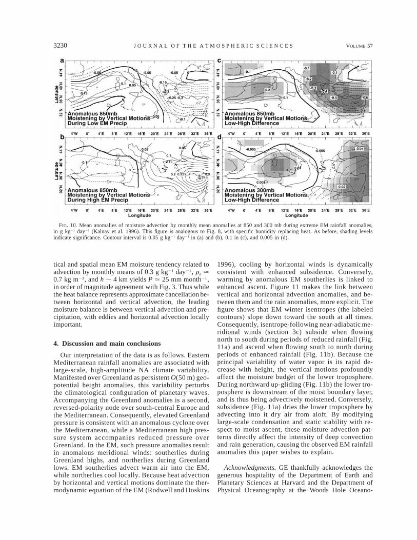
Unlike the thermodynamic equation, in which thesource term is generally small, the water vapor equa-tion contains a leading-order source term, the rainfallanomalies themselves. Three processes balance thesewater vapor anomalies. Horizontal moisture advectionby monthly mean anomalies (not shown; mostlyV · =qc where q is specific humidity) tends to havesmall spatial scales, and is generally relatively small.It tends to dry the EM during PL and moisten it duringPH , partially counteracting the rain anomalies. Whilealso secondary, moisture advection by eddies can beoccasionally locally important (e.g., over Turkey dur-ing PL , where they moisten at ,0.12 g kg21 day21).However, the leading term balancing EM moisture per-turbations is anomalous vertical moisture advectiondue to monthly mean anomalies, shown in Fig. 10. Asin the thermal equation, while Fig. 10 shows the fullanomaly, it is dominated by the interactions of theanomalous flow with the climatological moisture gra-dient, . Thus the approximate water vapor con-v] qp c
servation can be written ash r ]qa cP . 2 v dz, (6)E r ]pw0
where P is the precipitation rate in m day21, h is thethickness of the precipitating layer, and ra and rw denoteair and water densities. The rhs of Eq. (6) is the netimbalance between the water vapor mass advected intoand out of the precipitating layer. Because q values arevery small in the upper troposphere, even if conden-sation occurs there it contributes very little to the total-column precipitation (note the order of magnitude dropbetween Figs. 10c and 10d). Consequently, the rhs in-tegral can be truncated at a reasonable height abovewhich condensation yields insignificant liquid watermass; for the EM h . 4 km is roughly appropriate(which is the reason we concentrate mostly on the lowertroposphere in our analyses). Taking a characteristic ver-
3230 VOLUME 57J O U R N A L O F T H E A T M O S P H E R I C S C I E N C E S
FIG. 10. Mean anomalies of moisture advection by monthly mean anomalies at 850 and 300 mb during extreme EM rainfall anomalies,in g kg21 day21 (Kalnay et al. 1996). This figure is analogous to Fig. 8, with specific humidity replacing heat. As before, shading levelsindicate significance. Contour interval is 0.05 g kg21 day21 in (a) and (b), 0.1 in (c), and 0.005 in (d).
tical and spatial mean EM moisture tendency related toadvection by monthly means of 0.3 g kg21 day21, ra .0.7 kg m23, and h ; 4 km yields P . 25 mm month21,in order of magnitude agreement with Fig. 3. Thus whilethe heat balance represents approximate cancellation be-tween horizontal and vertical advection, the leadingmoisture balance is between vertical advection and pre-cipitation, with eddies and horizontal advection locallyimportant.
4. Discussion and main conclusions
Our interpretation of the data is as follows. EasternMediterranean rainfall anomalies are associated withlarge-scale, high-amplitude NA climate variability.Manifested over Greenland as persistent O(50 m) geo-potential height anomalies, this variability perturbsthe climatological configuration of planetary waves.Accompanying the Greenland anomalies is a second,reversed-polarity node over south-central Europe andthe Mediterranean. Consequently, elevated Greenlandpressure is consistent with an anomalous cyclone overthe Mediterranean, while a Mediterranean high pres-sure system accompanies reduced pressure overGreenland. In the EM, such pressure anomalies resultin anomalous meridional winds: southerlies duringGreenland highs, and northerlies during Greenlandlows. EM southerlies advect warm air into the EM,while northerlies cool locally. Because heat advectionby horizontal and vertical motions dominate the ther-modynamic equation of the EM (Rodwell and Hoskins
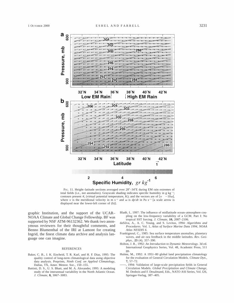
1996), cooling by horizontal winds is dynamicallyconsistent with enhanced subsidence. Conversely,warming by anomalous EM southerlies is linked toenhanced ascent. Figure 11 makes the link betweenvertical and horizontal advection anomalies, and be-tween them and the rain anomalies, more explicit. Thefigure shows that EM winter isentropes (the labeledcontours) slope down toward the south at all times.Consequently, isentrope-following near-adiabatic me-ridional winds (section 3c) subside when flowingnorth to south during periods of reduced rainfall (Fig.11a) and ascend when flowing south to north duringperiods of enhanced rainfall (Fig. 11b). Because theprincipal variability of water vapor is its rapid de-crease with height, the vertical motions profoundlyaffect the moisture budget of the lower troposphere.During northward up-gliding (Fig. 11b) the lower tro-posphere is downstream of the moist boundary layer,and is thus being advectively moistened. Conversely,subsidence (Fig. 11a) dries the lower troposphere byadvecting into it dry air from aloft. By modifyinglarge-scale condensation and static stability with re-spect to moist ascent, these moisture advection pat-terns directly affect the intensity of deep convectionand rain generation, causing the observed EM rainfallanomalies this paper wishes to explain.
Acknowledgments. GE thankfully acknowledges thegenerous hospitality of the Department of Earth andPlanetary Sciences at Harvard and the Department ofPhysical Oceanography at the Woods Hole Oceano-
1 OCTOBER 2000 3231E S H E L A N D F A R R E L L
FIG. 11. Height–latitude sections averaged over 288–348E during EM rain extremes oftotal fields (i.e., not anomalies). Grayscale shading indicates specific humidity in g kg21;contours present uy (virtual potential temperature, K); and the vectors are of [y 210v],where y is the meridional velocity in m s21 and v is dp/dt in Pa s21 [a scale arrow isdisplayed near the lower-left corner of (b)].
graphic Institution, and the support of the UCAR–NOAA Climate and Global Change Fellowship. BF wassupported by NSF ATM-96132362. We thank two anon-ymous reviewers for their thoughtful comments, andBenno Blumenthal of the IRI at Lamont for creatingIngrid, the finest climate data archive and analysis lan-guage one can imagine.
REFERENCES
Baker, C. B., J. K. Eischeid, T. R. Karl, and H. F. Diaz, 1995: Thequality control of long-term climatological data using objectivedata analysis. Preprints, Ninth Conf. on Applied Climatology,Dallas, TX, Amer. Meteor. Soc., 150–155.
Battisti, D. S., U. S. Bhatt, and M. A. Alexander, 1995: A modelingstudy of the interannual variability in the North Atlantic Ocean.J. Climate, 8, 3067–3083.
Blade, I., 1997: The influence of midlatitude ocean–atmosphere cou-pling on the low-frequency variability of a GCM. Part I: Notropical SST forcing. J. Climate, 10, 2087–2106.
daSilva, A., A. C. Young, and S. Levitus, 1994: Algorithms andProcedures. Vol. 1, Atlas of Surface Marine Data 1994, NOAAAtlas NESDIS 6.
Frankignoul, C., 1985: Sea surface temperature anomalies, planetarywaves, and air–sea feedback in the middle latitudes. Rev. Geo-phys., 23 (4), 357–390.
Holton, J. R., 1992: An Introduction to Dynamic Meteorology. 3d ed.International Geophysics Series, Vol. 48, Academic Press, 511pp.
Hulme, M., 1992: A 1951–80 global land precipitation climatologyfor the evaluation of General Circulation Models. Climate Dyn.,7, 57–72., 1994: Validation of large-scale precipitation fields in GeneralCirculation Models. Global Precipitation and Climate Change,M. Desbois and F. Desalmand, Eds., NATO ASI Series, Vol. I26,Springer-Verlag, 387–405.
3232 VOLUME 57J O U R N A L O F T H E A T M O S P H E R I C S C I E N C E S
Hurrell, J. W., 1995: Decadal trends in the North Atlantic oscillation:Regional temperatures and precipitation. Science, 269, 676–679., and H. van Loon, 1997: Decadal variations in climate associatedwith the North Atlantic oscillation. Climatic Change, 36, 301–326.
Kalnay, E., and Coauthors, 1996: The NCEP/NCAR 40-Year Re-analysis Project. Bull. Amer. Meteor. Soc., 77, 437–471.
Kushnir, Y., 1994: Interdecadal variations in North Atlantic sea sur-face temperature and associated atmospheric conditions. J. Cli-mate, 7, 141–157., 1999: Europe’s winter prospects. Nature, 398, 289–291., and J. M. Wallace, 1989: Low-frequency variability in theNorthern Hemisphere winter: Geographical distribution, struc-ture and timescale dependence. J. Atmos. Sci., 46, 3122–3142.
Latif, M., and T. P. Barnett, 1994: Causes of decadal variability overthe North Pacific and North America. Science, 266, 634–637., and , 1996: Decadal variability over the North Pacific andNorth America: Dynamics and predictability. J. Climate, 9,2407–2423.
McCartney, M. S., 1997: Is the ocean at the helm? Nature, 388, 521–522.
Molteni, F., and T. N. Palmer, 1993: Predictability and finite-timeinstability of the northern winter circulation. Quart. J. Roy. Me-teor. Soc., 119, 269–298.
Philips, J. L., 1982: How to Think about Statistics. Freeman andCompany Press, 198 pp.
Rodwell, M. J., and B. J. Hoskins, 1996: Monsoons and the dynamicsof deserts. Quart. J. Roy. Meteor. Soc., 122B, 1385–1404., D. P. Rowell, and C. K. Folland, 1999: Oceanic forcing of thewintertime North Atlantic Oscillation and European climate. Na-ture, 398, 320–323.
Steinberger, E. H., and N. Gazit-Yaari, 1996: Recent changes in thespatial distribution of annual precipitation in Israel. J. Climate,9, 3328–3336.
Trenberth, K. E., and C. J. Guillemot, 1998: Evaluation of the at-mospheric moisture and hydrological cycle in the NCEP/NCARreanalyses. Climate Dyn., 14, 213–231.
Venzke, S., M. R. Allen, R. T. Sutton, and D. P. Rowell, 1998: Theatmospheric response over the North Atlantic to decadal changesin sea surface temperature. Max-Planck-Institut fur MeteorologieRep. 255, 46 pp. [Available from Max-Planck-Institut fur Me-teorologie, Bundesstrasse 55, D-20146 Hamburg, F.R. Germany.]
Wallace, J. M., C. Smith, and Q. Jiang, 1990: Spatial patterns ofatmosphere–ocean interactions in the northern winter. J. Climate,3, 990–998., , and C. S. Bretherton, 1992: Singular value decompositionof wintertime sea surface temperature and 500-mb height anom-alies. J. Climate, 5, 561–576.
Weng, W., and J. D. Neelin, 1998: On the role of ocean–atmosphereinteraction in the midlatitude interdecadal variability. Geophys.Res. Lett., 25 (2), 167–170.