Embed Size (px)
Citation preview
HAL Id: hal-01408217https://hal.inria.fr/hal-01408217
Submitted on 3 Dec 2016
HAL is a multi-disciplinary open accessarchive for the deposit and dissemination of sci-entific research documents, whether they are pub-lished or not. The documents may come fromteaching and research institutions in France orabroad, or from public or private research centers.
L’archive ouverte pluridisciplinaire HAL, estdestinée au dépôt et à la diffusion de documentsscientifiques de niveau recherche, publiés ou non,émanant des établissements d’enseignement et derecherche français ou étrangers, des laboratoirespublics ou privés.
Mechanizing a Process Algebra for Network ProtocolsTimothy Bourke, Robert van Glabbeek, Peter Höfner
To cite this version:Timothy Bourke, Robert van Glabbeek, Peter Höfner. Mechanizing a Process Algebra for NetworkProtocols. Journal of Automated Reasoning, Springer Verlag, 2016, 56, pp.309-341. �10.1007/s10817-015-9358-9�. �hal-01408217�
Noname manuscript No.(will be inserted by the editor)
Mechanizing a Process Algebra for Network Protocols
Timothy Bourke · Robert J. van Glabbeek ·Peter Höfner
Received: date / Accepted: date
Abstract This paper presents the mechanization of a process algebra for Mo-bile Ad hoc Networks and Wireless Mesh Networks, and the development of acompositional framework for proving invariant properties. Mechanizing the coreprocess algebra in Isabelle/HOL is relatively standard, but its layered structurenecessitates special treatment. The control states of reactive processes, such asnodes in a network, are modelled by terms of the process algebra. We propose atechnique based on these terms to streamline proofs of inductive invariance. Thisis not sufficient, however, to state and prove invariants that relate states acrossmultiple processes (entire networks). To this end, we propose a novel composi-tional technique for lifting global invariants stated at the level of individual nodesto networks of nodes.
Keywords Interactive Theorem Proving · Isabelle/HOL · Process Algebra ·Compositional Invariant Proofs · Wireless Mesh Networks · Mobile Ad hocNetworks
1 Introduction and related work
The Algebra for Wireless Networks (AWN) is a process algebra developed in partic-ular for modelling and analysing protocols for Mobile Ad hoc Networks (MANETs)
NICTA is funded by the Australian Government through the Department of Communicationsand the Australian Research Council through the ICT Centre of Excellence Program.
T. BourkeInria Paris and École normale supérieure, Paris, FranceE-mail: [email protected]
R. J. van GlabbeekNICTA and UNSW, Sydney, AustraliaE-mail: [email protected]
P. HöfnerNICTA and UNSW, Sydney, AustraliaE-mail: [email protected]
2 Bourke, van Glabbeek, and Höfner
and Wireless Mesh Networks (WMNs) [10, 11], but that can be used for reason-ing about routing and communication protocols in general. This paper reportson both its mechanization in Isabelle/HOL [29] and the development of a com-positional framework for showing invariant properties of models.1 The techniqueswe describe are a response to problems encountered during the mechanization ofa model and proof of a crucial correctness property for the Ad hoc On-demandDistance Vector (AODV) routing protocol, a widely used protocol, standardizedby the IETF [31]. The AODV case study is described in detail elsewhere [5] andwe only refer to it briefly in this paper. The property we study is loop freedom,meaning that no data packet is sent in cycles forever. Such a property can only beexpressed by relating states of different (neighbouring) network nodes. Encodingsuch inter-node properties in an Interactive Theorem Prover (ITP) proved quitechallenging, since the proof is performed inductively for an arbitrary number ofnodes and the base case is a single node whose neighbours do not yet exist. Wedevelop a novel compositional technique to address this challenge.
Despite extensive research on related problems [34] and several mechanizedframeworks for reactive systems [9, 18, 27], we are not aware of other solutionsthat allow the compositional statement and proof of properties relating the statesof different nodes in a message-passing model—at least not within the stricturesimposed by an ITP.
Related work. AWN is a process algebra, but for the purposes of proving prop-erties we treat it essentially as a structured programming language and employa technique originally proposed by Floyd [13] and later developed by Manna andPnueli [23], whereby a set of semantic rules is defined to link the syntax of a pro-gram to an induced transition system. Safety properties are then shown to holdfor all reachable states by induction from a set of initial states over the set of tran-sitions. Rather than define the induced transition system in terms of labels and(virtual) program counters [23, Chapter 1], we use term derivatives and StructuralOperational Semantics (SOS) rules [32].
This separation between language and model differs from the approach takenin formalisms like UNITY [8] and I/O Automata [22], where initial states and setsof transitions are specified directly, and also from that of TLA+ [21], where theinitial states and transition relation are written as a formula of first-order logic.The advantage of the language-plus-semantics approach is that sequencing andbranching in models is expressed by syntactic operators with the implied changesin the underlying control state being managed by the semantic rules. Arguably,this permits models that are easier to understand by experts in the system beingmodelled. The disadvantage is some extra complexity and layers of definitions. Wefind, however, that these details are well managed by ITPs and—once defined—intrude little on the verification task.
AWN provides a unique mix of communication primitives and a treatment ofdata structures that are essential for studying MANET and WMN protocols withdynamic topologies and sophisticated routing logic [11, §1]. It supports commu-nication primitives for one-to-one (unicast), one-to-many (groupcast), and one-to-all(broadcast) message passing. AWN comprises distinct layers for expressing the struc-ture of nodes and networks. We exploit this structure critically in our proofs, and
1 The Isabelle/HOL source files can be found in the Archive of Formal Proofs (AFP) [4].
Mechanizing a Process Algebra for Network Protocols 3
we expect the techniques proposed in Sections 3 and 4 to also apply to similarlayered modelling languages [15,16,24,25,28,33].
Besides this, our work differs from other mechanizations for verifying reactivesystems, like UNITY [18], TLA+ [9], or I/O Automata [27] (from which we drewthe most inspiration), in its explicit treatment of control states, in the form ofprocess algebra terms, as distinct from data states. In this respect, our approach isclose to that of Isabelle/Circus [12], but it differs in (1) the treatment of operatorsfor composing nodes, which we model directly as functions on automata, (2) thetreatment of recursive invocations, which we do not permit, and (3) our inclusionof a framework for compositional proofs.
Within the process algebraic tradition, other work in ITPs focuses on showingproperties of process algebras, such as the treatment of binders [1], that bisimula-tion equivalence is a congruence [17, 19], or properties of fix-point induction [36],while we focus on what has been termed ‘proof methodology’ [14], and develop acompositional method for showing correctness properties of protocols specified ina process algebra.
As an alternative to the frameworks cited above, and the work we present,Paulson’s inductive approach [30] can be applied to show properties of protocolsspecified with less generic infrastructure. In fact, it has also been applied to modelthe AODV protocol [39]; a detailed comparison is given elsewhere [5, §9]. Butwe think this approach to be better suited to systems specified in a ‘declarative’style as opposed to the strongly operational models we consider. The question ofstyle has practical implications. It determines the ‘distance’ between the originalspecification and the formal model—perhaps surprisingly protocol descriptions areoften quite operational (this is the case for AODV [31]). It also likely influencesproofs of refinement between abstract and implementation models.
Structure and contributions. Section 2 describes the mechanization of AWN. Thebasic definitions are routine but the layered structure of the language and thetreatment of operators on networks as functions on automata are relatively noveland essential to understanding later sections. Section 3 describes our mechaniza-tion of the theory of inductive invariants, closely following [23]. We exploit thestructure of AWN to generate verification conditions corresponding to those ofpen-and-paper proofs [11, §7]. Section 4 presents a compositional technique forstating and proving invariants that relate states across multiple nodes. Basically,we substitute ‘open’ SOS rules over the global state for the standard rules overlocal states (Section 4.1), show the property over a single sequential process (Sec-tion 4.2), ‘lift’ it successively over layers that model message queueing and networkcommunication (Section 4.3), and, ultimately, ‘transfer’ it to the original model(Section 4.4).
Note. This paper is an extended version of [6]. It presents all details with regardsto the mechanization—many of which were skipped in [6] due to lack of space. Wealso present more details about the novel compositional technique for lifting globalinvariants, including motivation and examples. As a case study, the framework wepresent in this paper was successfully applied in the mechanization of a proofof AODV’s loop freedom, the details of which are available in the AFP [7] andpresented elsewhere [5].
4 Bourke, van Glabbeek, and Höfner
{l}[[u]] p ’l ⇒ (’k ⇒ ’k) ⇒ (’k, ’p, ’l) seqp ⇒ (’k, ’p, ’l) seqp{l}〈g〉 p ’l ⇒ (’k ⇒ ’k set) ⇒ (’k, ’p, ’l) seqp ⇒ (’k, ’p, ’l) seqp{l}unicast(sid , smsg ) . p . q ’l ⇒ (’k ⇒ ip) ⇒ (’k ⇒ msg) ⇒ (’k, ’p, ’l) seqp ⇒
(’k, ’p, ’l) seqp ⇒ (’k, ’p, ’l) seqp{l}broadcast(smsg ) . p ’l ⇒ (’k ⇒ msg) ⇒ (’k, ’p, ’l) seqp ⇒ (’k, ’p, ’l) seqp{l}groupcast(sids , smsg ) . p ’l ⇒ (’k ⇒ ip set) ⇒ (’k ⇒ msg) ⇒ (’k, ’p, ’l) seqp ⇒
(’k, ’p, ’l) seqp{l}send(smsg ) . p ’l ⇒ (’k ⇒ msg) ⇒ (’k, ’p, ’l) seqp ⇒ (’k, ’p, ’l) seqp{l}receive(umsg ) . p ’l ⇒ (msg ⇒ ’k ⇒ ’k) ⇒ (’k, ’p, ’l) seqp ⇒ (’k, ’p, ’l) seqp{l}deliver(sdata ) . p ’l ⇒ (’k ⇒ data) ⇒ (’k, ’p, ’l) seqp ⇒ (’k, ’p, ’l) seqpp ⊕ q (’k, ’p, ’l) seqp ⇒ (’k, ’p, ’l) seqp ⇒ (’k, ’p, ’l) seqpcall(pn) ’p ⇒ (’k, ’p, ’l) seqp
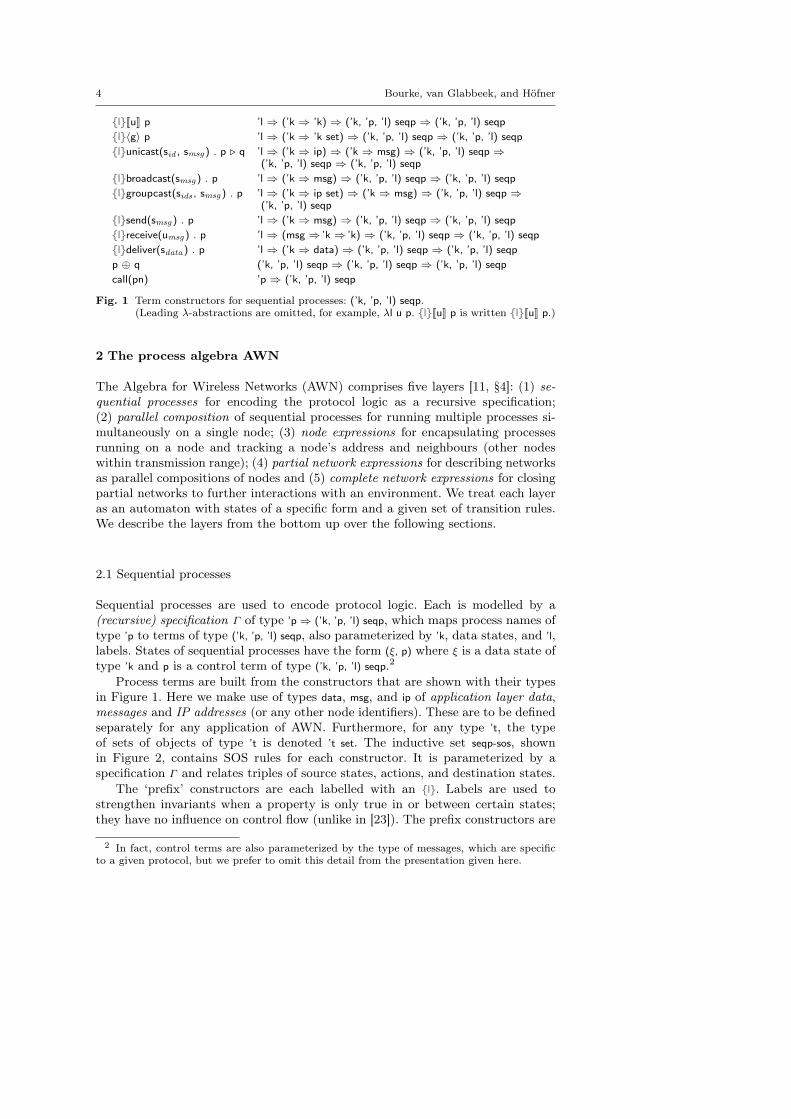
Fig. 1 Term constructors for sequential processes: (’k, ’p, ’l) seqp.(Leading λ-abstractions are omitted, for example, λl u p. {l}[[u]] p is written {l}[[u]] p.)
2 The process algebra AWN
The Algebra for Wireless Networks (AWN) comprises five layers [11, §4]: (1) se-quential processes for encoding the protocol logic as a recursive specification;(2) parallel composition of sequential processes for running multiple processes si-multaneously on a single node; (3) node expressions for encapsulating processesrunning on a node and tracking a node’s address and neighbours (other nodeswithin transmission range); (4) partial network expressions for describing networksas parallel compositions of nodes and (5) complete network expressions for closingpartial networks to further interactions with an environment. We treat each layeras an automaton with states of a specific form and a given set of transition rules.We describe the layers from the bottom up over the following sections.
2.1 Sequential processes
Sequential processes are used to encode protocol logic. Each is modelled by a(recursive) specification Γ of type ’p⇒ (’k, ’p, ’l) seqp, which maps process names oftype ’p to terms of type (’k, ’p, ’l) seqp, also parameterized by ’k, data states, and ’l,labels. States of sequential processes have the form (ξ, p) where ξ is a data state oftype ’k and p is a control term of type (’k, ’p, ’l) seqp.2
Process terms are built from the constructors that are shown with their typesin Figure 1. Here we make use of types data, msg, and ip of application layer data,messages and IP addresses (or any other node identifiers). These are to be definedseparately for any application of AWN. Furthermore, for any type ’t, the typeof sets of objects of type ’t is denoted ’t set. The inductive set seqp-sos, shownin Figure 2, contains SOS rules for each constructor. It is parameterized by aspecification Γ and relates triples of source states, actions, and destination states.
The ‘prefix’ constructors are each labelled with an {l}. Labels are used tostrengthen invariants when a property is only true in or between certain states;they have no influence on control flow (unlike in [23]). The prefix constructors are
2 In fact, control terms are also parameterized by the type of messages, which are specificto a given protocol, but we prefer to omit this detail from the presentation given here.

Mechanizing a Process Algebra for Network Protocols 5
ξ’ = u ξ((ξ, {l}[[u]] p), τ , (ξ’, p))∈ seqp-sos Γ
ξ’∈ g ξ((ξ, {l}〈g〉 p), τ , (ξ’, p))∈ seqp-sos Γ
((ξ, {l}unicast(sid , smsg ) . p . q), unicast (sid ξ) (smsg ξ), (ξ, p))∈ seqp-sos Γ
((ξ, {l}unicast(sid , smsg ) . p . q), ¬unicast (sid ξ), (ξ, q))∈ seqp-sos Γ
((ξ, {l}broadcast(smsg ) . p), broadcast (smsg ξ), (ξ, p))∈ seqp-sos Γ
((ξ, {l}groupcast(sids , smsg ) . p), groupcast (sids ξ) (smsg ξ), (ξ, p))∈ seqp-sos Γ
((ξ, {l}send(smsg ) . p), send (smsg ξ), (ξ, p))∈ seqp-sos Γ
((ξ, {l}receive(umsg ) . p), receive msg, (umsg msg ξ, p))∈ seqp-sos Γ
((ξ, {l}deliver(sdata ) . p), deliver (sdata ξ), (ξ, p))∈ seqp-sos Γ
((ξ, p), a, (ξ’, p’))∈ seqp-sos Γ((ξ, p ⊕ q), a, (ξ’, p’))∈ seqp-sos Γ
((ξ, q), a, (ξ’, q’))∈ seqp-sos Γ((ξ, p ⊕ q), a, (ξ’, q’))∈ seqp-sos Γ
((ξ, Γ pn), a, (ξ’, p’))∈ seqp-sos Γ((ξ, call(pn)), a, (ξ’, p’))∈ seqp-sos Γ
Fig. 2 SOS rules for sequential processes: seqp-sos.
assignment, guard/bind, network synchronizations unicast/broadcast/groupcast/receive,and internal communications send/receive/deliver.
The assignment {l}[[u]] p transforms the data state ξ deterministically into thedata state ξ’, according to the function u, and then acts as p. ‘During’ the updatea τ-action is performed. In the original AWN [10,11], the data state ξ was definedas a partial function from data variables to values of the appropriate type, and theassignment u modified or extended this partial function by (re)mapping a specificvariable to a new value, which could depend on the current data state. In ourmechanization the type of data states is given as an abstract parameter of thelanguage that is not yet instantiated in any particular way. Consequently, u istaken to be any function of type ’k ⇒ ’k, modifying the data state. In comparisonwith [10,11], our current treatment is less syntactic and more general.
The guard/bind statement {l}〈g〉 p encodes both guards and variable bindings.Here g is of type ’k⇒ ’k set, a function from data states to sets of data states. Execut-ing a guard amounts to making a nondeterministic choice of one of the data statesobtainable from the current state ξ by applying g; in case g(ξ) is empty no transi-tion is possible. For a valuation function h of type ’k ⇒ bool the guard statementis implemented as {l}〈λξ. if h ξ then {ξ} else ∅〉 p, which has no outgoing transitionif h evaluates to false. Variable binding like 〈λξ. {ξ(|no := n|) | n < 5}〉 p returns allpossible states that satisfy the binding constraint. In the original AWN [10, 11],where the data state ξ was a partial function from data variables to values, theexecution of a guard/bind construct could only extend the domain of ξ, therebyassigning values to previously unbound variables. In our more abstract approachto data states, we must allow any manipulation of the (as of yet unspecified) datastate. As this includes changing values of already bound variables, the guard/bindconstruct strictly subsumes assignment. Since this ‘misuse’ of a guard as assign-
6 Bourke, van Glabbeek, and Höfner
ment is not allowed in the original semantics of AWN [10, 11], we prefer to keepboth.
The sequential process {l}unicast(sid , smsg ) . p . q tries to unicast the message smsg
to the destination sid ; if successful it continues to act as p and otherwise as q. Inother words, unicast(sid , smsg ) . p is prioritized over q, which is only considered whenthe unicast action is not possible (¬unicast (sid ξ)). Which of the actions unicast or¬unicast will occur depends on whether the destination sid is in transmission rangeof the current node; this is implemented by the first two rules of Figure 7 (describedlater). In [10,11] the message smsg is an expression with variables that evaluates to amessage depending on the current values of those variables. Here, more abstractly,it can be any function of type ’k⇒ msg that constructs a message from the currentdata state. The sequential process {l}broadcast(smsg ) . p broadcasts smsg to the othernetwork nodes within transmission range.3 The process {l}groupcast(sids , smsg ) . ptries to transmit smsg to all destinations sids , and proceeds as p regardless of whetherany of the transmissions is successful.
The sequential process {l}send(smsg ) . p synchronously transmits a message toanother process running on the same network node; this action can occur only whenthe other sequential process is able to receive the message. The sequential process{l}receive(umsg ) . p receives any message umsg either from another node, from anothersequential process running on the same node, or from the client4 connected to thelocal node. It then proceeds as p, but with an updated data state (the state changeis triggered by the message). In the original syntax and semantics of AWN, umsg
was a data variable of type msg; here it is an abstract function of type msg⇒ ’k⇒ ’k,which changes the data state. The submission of data from a client is modelled bythe receipt of a special message (Newpkt d dst), where the function Newpkt generatesa message containing the data d and the intended destination dst. Data is deliveredto the client by {l}deliver(sdata ) . p.
The other constructors are unlabelled and serve to ‘glue’ processes together:The choice construct p ⊕ q takes the union of two transition sets and hence mayact either as p or as q. The procedure call call(pn) affixes a term from the specifica-tion (Γ pn). The behaviour of call(pn) is exactly the same as that of the sequentialprocess that Γ associates to the process name pn. In [10, 11], on the other hand,process names pn are explicitly parameterized with a list of data variables whichcan be defined by arbitrary data expressions at the call site. The semantics of theprocess call involves running the process Γ pn on an updated data state, obtainedby evaluating the data expressions in the current state and assigning the result-ing values to the corresponding variables, while clearing the values of all variablesthat do not occur as parameters of pn, effectively making them undefined. In thecurrent treatment, this behaviour is recovered by preceding a call(pn) by an explicitassignment statement. As variables cannot be made undefined, they are clearedby setting them to arbitrary values. This change is the biggest departure fromthe original definition of AWN; it simplifies the treatment of call, as we show inSection 3.1, and facilitates working with automata where variable locality makeslittle sense. The drawback is that the atomic ‘assign and jump’ semantics is lost,which is sometimes inconvenient (an example is given later in Section 2.2).
3 Whether a node is within transmission range or not is determined later on.4 The application layer that initiates packet sending and awaits receipt of a packet.
Mechanizing a Process Algebra for Network Protocols 7
ΓToy PToy = labelled PToy ( receive(λmsg’ ξ. ξ (| msg := msg’ |)). {PToy-:0}
[[λξ. ξ (|nhid := id ξ|)]] {PToy-:1}
( 〈is-newpkt〉 {PToy-:2}
[[λξ. ξ (|no := max (no ξ) (num ξ)|)]] {PToy-:3}
broadcast(λξ. Pkt (no ξ) (id ξ)). {PToy-:4}
[[clear-locals]] call(PToy) {PToy-:5}
⊕ 〈is-pkt〉 {PToy-:2}
( 〈λξ. if num ξ > no ξ then {ξ} else ∅〉 {PToy-:6}
[[λξ. ξ (|no := num ξ|)]] {PToy-:7}
[[λξ. ξ (|nhid := sid ξ|)]] {PToy-:8}
broadcast(λξ. Pkt (no ξ) (id ξ)). {PToy-:9}
[[clear-locals]] call(PToy) {PToy-:10}
⊕ 〈λξ. if num ξ ≤ no ξ then {ξ} else ∅〉 {PToy-:6}
[[clear-locals]] call(PToy)))) {PToy-:11}
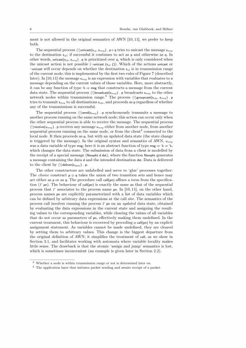
Fig. 3 AWN-specification of a toy protocol.
An example sequential process. We give the specification of a simple ‘toy’ proto-col as a running example. The formal AWN specification is presented in Figure 3.Nodes following the protocol broadcast messages containing an integer no. Each re-members the largest integer it has received and drops messages containing smalleror equal values.
The protocol is defined by a process named PToy that maintains three variables:the integer no; an identifier id—also an integer, which uniquely identifies a node (forexample, the node’s IP address); and an identifier nhid that stores a node address(either that of the node itself, or the address of another node that supplied thelargest number in the last comparison it made).5 The initial values of nhid and noare id and 0, respectively.
The behaviour of a single node in our toy protocol is given by the recursivespecification ΓToy and an initial state (ξ, p) consisting of a data state ξ—definedabove—and a control term p—here the process ΓToy PToy. The specification ΓToy,given in Figure 3, assigns a process term to each process name—here only to thename PToy. The process term ΓToy PToy is defined as the result of applying a func-tion labelled to two arguments: an identifier and the actual process without labels.The labels are supplied by the function labelled: it associates its first argumentpaired with a number as a label to every prefix construct occurring as a subterm.We show these labels on the right-hand side of Figure 3. Note that the choice con-struct ⊕ and the subterms call(PToy) do not receive a label. Moreover, the functionlabelled is defined in such a way that both arguments of the ⊕ receive the samelabel; this way labels correspond exactly to states that can be reached during theexecution of the process.
A node id running the protocol PToy will wait until it receives a message msg’(line {PToy-:0}). The protocol then updates the local data state ξ by assigning themessage msg’ to the variable msg (λξ. ξ (| msg := msg’ |)). In our scenario, there aretwo message constructors Pkt d src and Newpkt d dst; both carry an identifier (src anddst) and an integer-payload d. Here, src is, by design, the sender of the message. Werequire that all messages from the client of a node must have the form Newpkt d dst.
5 The protocol behaviour regarding nhid is rather arbitrary; it only serves to illustrate someforthcoming concepts.
8 Bourke, van Glabbeek, and Höfner
PToy
{PToy-:0}
{PToy-:1}
{PToy-:2}
{PToy-:3}
{PToy-:4}
{PToy-:5}
broadcast
[[· · · ]]
〈· · · 〉
{PToy-:6}
{PToy-:7}
{PToy-:8}
{PToy-:9}
{PToy-:10}
broadcast
[[· · · ]]
[[· · · ]]
〈· · · 〉
{PToy-:11}
〈· · · 〉
〈· · · 〉
[[· · · ]]
receive
[[· · · ]]
[[· · · ]]
[[· · · ]]
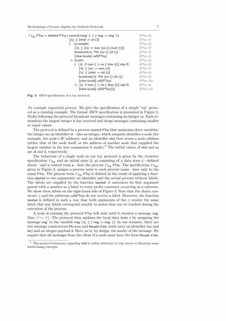
Fig. 4 Control state structure of ΓToy.
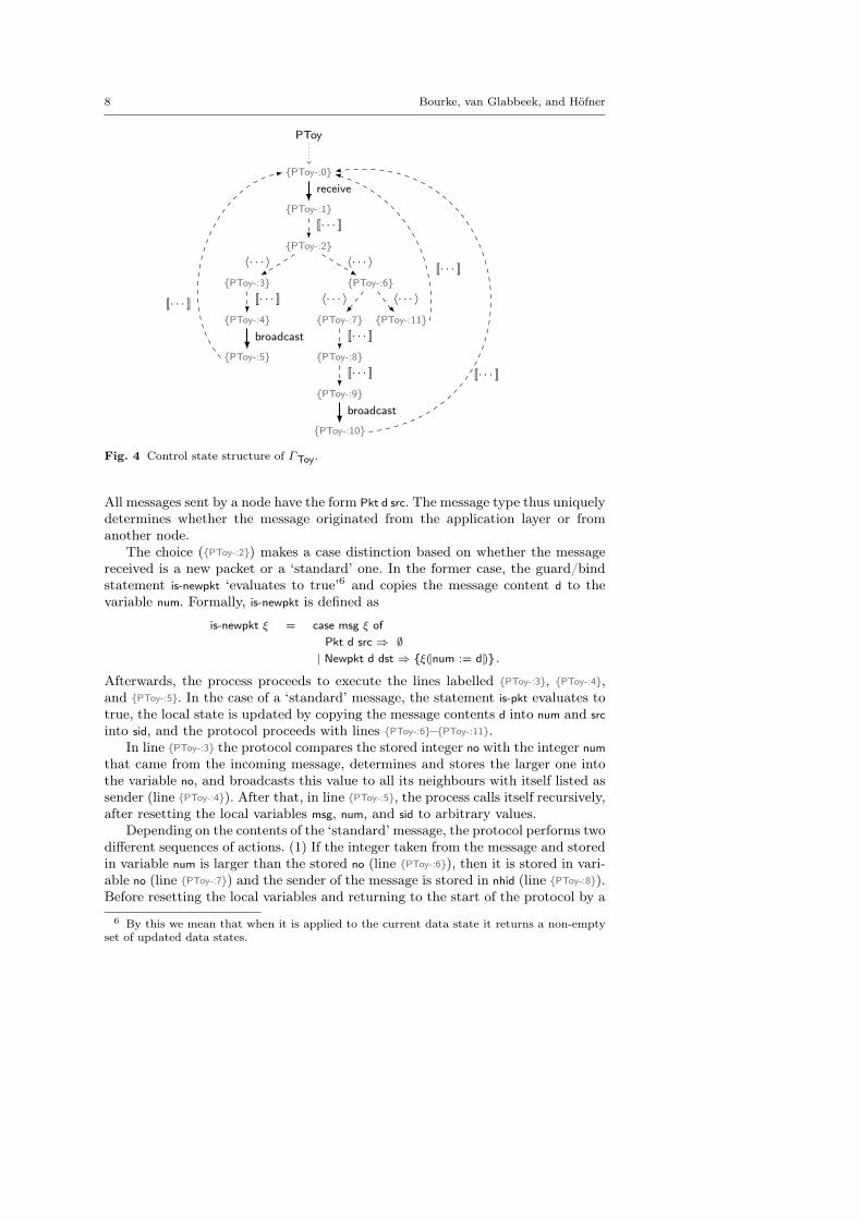
All messages sent by a node have the form Pkt d src. The message type thus uniquelydetermines whether the message originated from the application layer or fromanother node.
The choice ({PToy-:2}) makes a case distinction based on whether the messagereceived is a new packet or a ‘standard’ one. In the former case, the guard/bindstatement is-newpkt ‘evaluates to true’6 and copies the message content d to thevariable num. Formally, is-newpkt is defined as
is-newpkt ξ = case msg ξ ofPkt d src ⇒ ∅
| Newpkt d dst ⇒ {ξ(|num := d|)} .
Afterwards, the process proceeds to execute the lines labelled {PToy-:3}, {PToy-:4},and {PToy-:5}. In the case of a ‘standard’ message, the statement is-pkt evaluates totrue, the local state is updated by copying the message contents d into num and srcinto sid, and the protocol proceeds with lines {PToy-:6}–{PToy-:11}.
In line {PToy-:3} the protocol compares the stored integer no with the integer numthat came from the incoming message, determines and stores the larger one intothe variable no, and broadcasts this value to all its neighbours with itself listed assender (line {PToy-:4}). After that, in line {PToy-:5}, the process calls itself recursively,after resetting the local variables msg, num, and sid to arbitrary values.
Depending on the contents of the ‘standard’ message, the protocol performs twodifferent sequences of actions. (1) If the integer taken from the message and storedin variable num is larger than the stored no (line {PToy-:6}), then it is stored in vari-able no (line {PToy-:7}) and the sender of the message is stored in nhid (line {PToy-:8}).Before resetting the local variables and returning to the start of the protocol by a
6 By this we mean that when it is applied to the current data state it returns a non-emptyset of updated data states.
Mechanizing a Process Algebra for Network Protocols 9
Γqmsg Qmsg = labelled Qmsg (receive(λmsg msgs. msgs @ [msg]) . call(Qmsg) {Qmsg-:0}
⊕ 〈λmsgs. if msgs 6= [ ] then {msgs} else ∅〉 {Qmsg-:0}
( send(λmsgs. hd msgs) . {Qmsg-:1}
( [[λmsgs. tl msgs]] call(Qmsg) {Qmsg-:2}
⊕ receive(λmsg msgs. tl msgs @ [msg]) . call(Qmsg)) {Qmsg-:2}
⊕ receive(λmsg msgs. msgs @ [msg]) . call(Qmsg))) {Qmsg-:1}
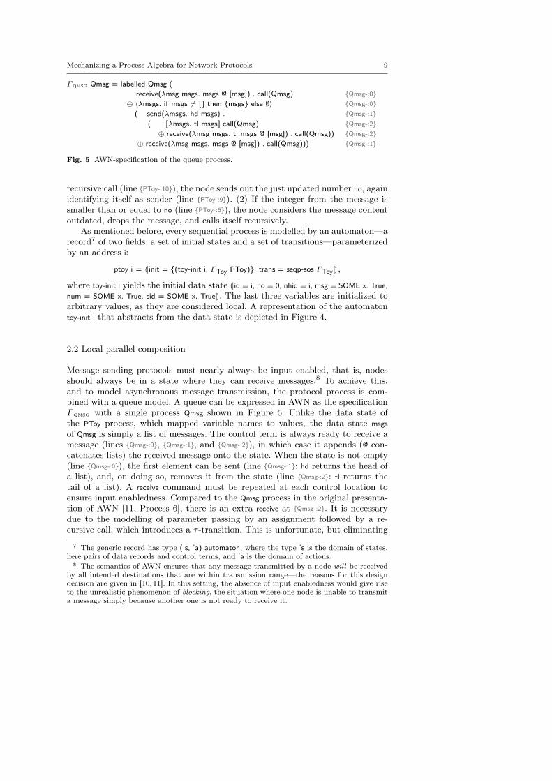
Fig. 5 AWN-specification of the queue process.
recursive call (line {PToy-:10}), the node sends out the just updated number no, againidentifying itself as sender (line {PToy-:9}). (2) If the integer from the message issmaller than or equal to no (line {PToy-:6}), the node considers the message contentoutdated, drops the message, and calls itself recursively.
As mentioned before, every sequential process is modelled by an automaton—arecord7 of two fields: a set of initial states and a set of transitions—parameterizedby an address i:
ptoy i = (|init = {(toy-init i, ΓToy PToy)}, trans = seqp-sos ΓToy|) ,
where toy-init i yields the initial data state (|id = i, no = 0, nhid = i, msg = SOME x. True,num = SOME x. True, sid = SOME x. True|). The last three variables are initialized toarbitrary values, as they are considered local. A representation of the automatontoy-init i that abstracts from the data state is depicted in Figure 4.
2.2 Local parallel composition
Message sending protocols must nearly always be input enabled, that is, nodesshould always be in a state where they can receive messages.8 To achieve this,and to model asynchronous message transmission, the protocol process is com-bined with a queue model. A queue can be expressed in AWN as the specificationΓ qmsg with a single process Qmsg shown in Figure 5. Unlike the data state ofthe PToy process, which mapped variable names to values, the data state msgsof Qmsg is simply a list of messages. The control term is always ready to receive amessage (lines {Qmsg-:0}, {Qmsg-:1}, and {Qmsg-:2}), in which case it appends (@ con-catenates lists) the received message onto the state. When the state is not empty(line {Qmsg-:0}), the first element can be sent (line {Qmsg-:1}: hd returns the head ofa list), and, on doing so, removes it from the state (line {Qmsg-:2}: tl returns thetail of a list). A receive command must be repeated at each control location toensure input enabledness. Compared to the Qmsg process in the original presenta-tion of AWN [11, Process 6], there is an extra receive at {Qmsg-:2}. It is necessarydue to the modelling of parameter passing by an assignment followed by a re-cursive call, which introduces a τ -transition. This is unfortunate, but eliminating
7 The generic record has type (’s, ’a) automaton, where the type ’s is the domain of states,here pairs of data records and control terms, and ’a is the domain of actions.
8 The semantics of AWN ensures that any message transmitted by a node will be receivedby all intended destinations that are within transmission range—the reasons for this designdecision are given in [10, 11]. In this setting, the absence of input enabledness would give riseto the unrealistic phenomenon of blocking, the situation where one node is unable to transmita message simply because another one is not ready to receive it.
10 Bourke, van Glabbeek, and Höfner
(s, a, s’)∈TA∧m. a 6= receive m
((s, t), a, (s’, t))∈ parp-sos TA TB
(t, a, t’)∈TB∧m. a 6= send m
((s, t), a, (s, t’))∈ parp-sos TA TB
(s, receive m, s’)∈TA (t, send m, t’)∈TB
((s, t), τ , (s’, t’))∈ parp-sos TA TB
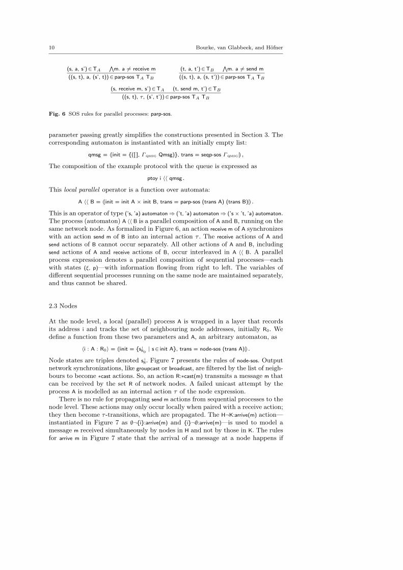
Fig. 6 SOS rules for parallel processes: parp-sos.
parameter passing greatly simplifies the constructions presented in Section 3. Thecorresponding automaton is instantiated with an initially empty list:
qmsg = (|init = {([ ], Γqmsg Qmsg)}, trans = seqp-sos Γqmsg|) ,
The composition of the example protocol with the queue is expressed as
ptoy i 〈〈 qmsg .
This local parallel operator is a function over automata:
A 〈〈 B = (|init = init A × init B, trans = parp-sos (trans A) (trans B)|) .
This is an operator of type (’s, ’a) automaton⇒ (’t, ’a) automaton⇒ (’s × ’t, ’a) automaton.The process (automaton) A 〈〈 B is a parallel composition of A and B, running on thesame network node. As formalized in Figure 6, an action receive m of A synchronizeswith an action send m of B into an internal action τ . The receive actions of A andsend actions of B cannot occur separately. All other actions of A and B, includingsend actions of A and receive actions of B, occur interleaved in A 〈〈 B. A parallelprocess expression denotes a parallel composition of sequential processes—eachwith states (ξ, p)—with information flowing from right to left. The variables ofdifferent sequential processes running on the same node are maintained separately,and thus cannot be shared.
2.3 Nodes
At the node level, a local (parallel) process A is wrapped in a layer that recordsits address i and tracks the set of neighbouring node addresses, initially R0. Wedefine a function from these two parameters and A, an arbitrary automaton, as
〈i : A : R0〉 = (|init = {s iR0
| s∈ init A}, trans = node-sos (trans A)|) .
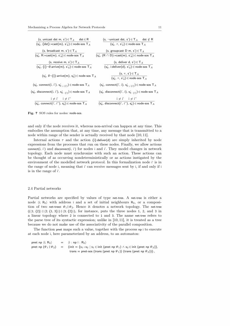
Node states are triples denoted s iR. Figure 7 presents the rules of node-sos. Output
network synchronizations, like groupcast or broadcast, are filtered by the list of neigh-bours to become ∗cast actions. So, an action R:∗cast(m) transmits a message m thatcan be received by the set R of network nodes. A failed unicast attempt by theprocess A is modelled as an internal action τ of the node expression.
There is no rule for propagating send m actions from sequential processes to thenode level. These actions may only occur locally when paired with a receive action;they then become τ -transitions, which are propagated. The H¬K:arrive(m) action—instantiated in Figure 7 as ∅¬{i}:arrive(m) and {i}¬∅:arrive(m)—is used to model amessage m received simultaneously by nodes in H and not by those in K. The rulesfor arrive m in Figure 7 state that the arrival of a message at a node happens if
Mechanizing a Process Algebra for Network Protocols 11
(s, unicast dst m, s’)∈TA dst∈R(s i
R, {dst}:∗cast(m), s’ iR)∈ node-sos TA
(s, ¬unicast dst, s’)∈TA dst /∈ R(s i
R, τ , s’iR)∈ node-sos TA
(s, broadcast m, s’)∈TA
(s iR, R:∗cast(m), s’ iR)∈ node-sos TA
(s, groupcast D m, s’)∈TA
(s iR, (R ∩ D):∗cast(m), s’ iR)∈ node-sos TA
(s, receive m, s’)∈TA
(s iR, {i}¬∅:arrive(m), s’ iR)∈ node-sos TA
(s, deliver d, s’)∈TA
(s iR, i:deliver(d), s’
iR)∈ node-sos TA
(s iR, ∅¬{i}:arrive(m), s i
R)∈ node-sos TA(s, τ , s’)∈TA
(s iR, τ , s’
iR)∈ node-sos TA
(s iR, connect(i, i’), s i
R ∪ {i’})∈ node-sos TA (s iR, connect(i’, i), s i
R ∪ {i’})∈ node-sos TA
(s iR, disconnect(i, i’), s i
R - {i’})∈ node-sos TA (s iR, disconnect(i’, i), s i
R - {i’})∈ node-sos TA
i 6= i’ i 6= i’’(s i
R, connect(i’, i’’), siR)∈ node-sos TA
i 6= i’ i 6= i’’(s i
R, disconnect(i’, i’’), siR)∈ node-sos TA
Fig. 7 SOS rules for nodes: node-sos.
and only if the node receives it, whereas non-arrival can happen at any time. Thisembodies the assumption that, at any time, any message that is transmitted to anode within range of the sender is actually received by that node [10,11].
Internal actions τ and the action {i}:deliver(d) are simply inherited by nodeexpressions from the processes that run on these nodes. Finally, we allow actionsconnect(i, i’) and disconnect(i, i’) for nodes i and i’. They model changes in networktopology. Each node must synchronize with such an action. These actions canbe thought of as occurring nondeterministically or as actions instigated by theenvironment of the modelled network protocol. In this formalization node i’ is inthe range of node i, meaning that i’ can receive messages sent by i, if and only if iis in the range of i’.
2.4 Partial networks
Partial networks are specified by values of type net-tree. A net-tree is either anode 〈i; R0〉 with address i and a set of initial neighbours R0, or a composi-tion of two net-trees Ψ1‖Ψ2. Hence it denotes a network topology. The net-tree((〈1; {2}〉 ‖ 〈2; {1, 3}〉) ‖ 〈3; {2}〉), for instance, puts the three nodes 1, 2, and 3 ina linear topology where 2 is connected to 1 and 3. The name net-tree refers tothe parse tree of its syntactic expression; unlike in [10, 11], it is treated as a treebecause we do not make use of the associativity of the parallel composition.
The function pnet maps such a value, together with the process np i to executeat each node i, here parameterized by an address, to an automaton:
pnet np 〈i; R0〉 = 〈i : np i : R0〉pnet np (Ψ1 ‖Ψ2) = (|init = {s1 q s2 | s1 ∈ init (pnet np Ψ1) ∧ s2 ∈ init (pnet np Ψ2)},
trans = pnet-sos (trans (pnet np Ψ1)) (trans (pnet np Ψ2))|) ,
12 Bourke, van Glabbeek, and Höfner
(s, R:∗cast(m), s’)∈TA (t, H¬K:arrive(m), t’)∈TB H ⊆ R K ∩ R = ∅(s q t, R:∗cast(m), s’q t’)∈ pnet-sos TA TB
(s, H¬K:arrive(m), s’)∈TA (t, R:∗cast(m), t’)∈TB H ⊆ R K ∩ R = ∅(s q t, R:∗cast(m), s’q t’)∈ pnet-sos TA TB
(s, H¬K:arrive(m), s’)∈TA (t, H’¬K’:arrive(m), t’)∈TB
(s q t, (H ∪ H’)¬(K ∪ K’):arrive(m), s’q t’)∈ pnet-sos TA TB
(s, i:deliver(d), s’)∈TA
(s q t, i:deliver(d), s’q t)∈ pnet-sos TA TB
(t, i:deliver(d), t’)∈TB
(s q t, i:deliver(d), s q t’)∈ pnet-sos TA TB
(s, τ , s’)∈TA
(s q t, τ , s’q t)∈ pnet-sos TA TB
(t, τ , t’)∈TB
(s q t, τ , s q t’)∈ pnet-sos TA TB
(s, connect(i, i’), s’)∈TA (t, connect(i, i’), t’)∈TB
(s q t, connect(i, i’), s’q t’)∈ pnet-sos TA TB
(s, disconnect(i, i’), s’)∈TA (t, disconnect(i, i’), t’)∈TB
(s q t, disconnect(i, i’), s’q t’)∈ pnet-sos TA TB
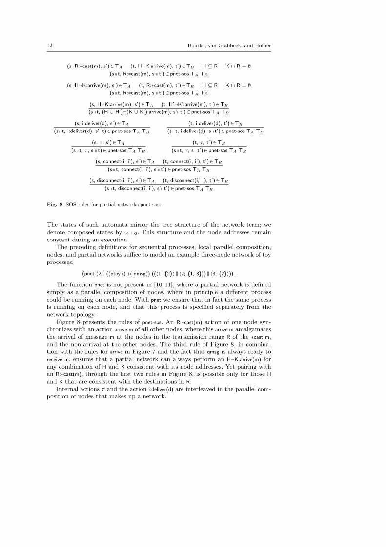
Fig. 8 SOS rules for partial networks pnet-sos.
The states of such automata mirror the tree structure of the network term; wedenote composed states by s1q s2. This structure and the node addresses remainconstant during an execution.
The preceding definitions for sequential processes, local parallel composition,nodes, and partial networks suffice to model an example three-node network of toyprocesses:
(pnet (λi. ((ptoy i) 〈〈 qmsg)) ((〈1; {2}〉 ‖ 〈2; {1, 3}〉) ‖ 〈3; {2}〉)) .
The function pnet is not present in [10, 11], where a partial network is definedsimply as a parallel composition of nodes, where in principle a different processcould be running on each node. With pnet we ensure that in fact the same processis running on each node, and that this process is specified separately from thenetwork topology.
Figure 8 presents the rules of pnet-sos. An R:∗cast(m) action of one node syn-chronizes with an action arrive m of all other nodes, where this arrive m amalgamatesthe arrival of message m at the nodes in the transmission range R of the ∗cast m,and the non-arrival at the other nodes. The third rule of Figure 8, in combina-tion with the rules for arrive in Figure 7 and the fact that qmsg is always ready toreceive m, ensures that a partial network can always perform an H¬K:arrive(m) forany combination of H and K consistent with its node addresses. Yet pairing withan R:∗cast(m), through the first two rules in Figure 8, is possible only for those Hand K that are consistent with the destinations in R.
Internal actions τ and the action i:deliver(d) are interleaved in the parallel com-position of nodes that makes up a network.
Mechanizing a Process Algebra for Network Protocols 13
(s, connect(i, i’), s’)∈TA
(s, connect(i, i’), s’)∈ cnet-sos TA
(s, disconnect(i, i’), s’)∈TA
(s, disconnect(i, i’), s’)∈ cnet-sos TA
(s, R:∗cast(m), s’)∈TA
(s, τ , s’)∈ cnet-sos TA
(s, τ , s’)∈TA
(s, τ , s’)∈ cnet-sos TA
(s, i:deliver(d), s’)∈TA
(s, i:deliver(d), s’)∈ cnet-sos TA
(s, {i}¬K:arrive(Newpkt d dst), s’)∈TA
(s, i:newpkt(d, dst), s’)∈ cnet-sos TA
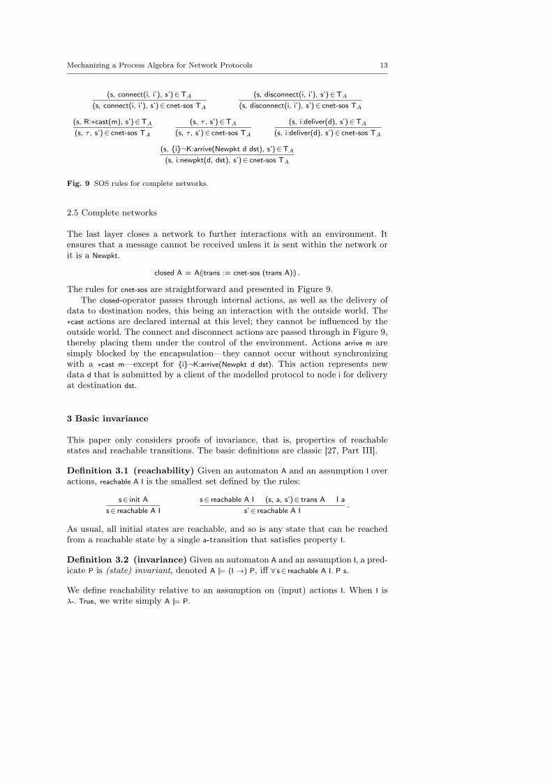
Fig. 9 SOS rules for complete networks.
2.5 Complete networks
The last layer closes a network to further interactions with an environment. Itensures that a message cannot be received unless it is sent within the network orit is a Newpkt.
closed A = A(|trans := cnet-sos (trans A)|) .
The rules for cnet-sos are straightforward and presented in Figure 9.The closed-operator passes through internal actions, as well as the delivery of
data to destination nodes, this being an interaction with the outside world. The∗cast actions are declared internal at this level; they cannot be influenced by theoutside world. The connect and disconnect actions are passed through in Figure 9,thereby placing them under the control of the environment. Actions arrive m aresimply blocked by the encapsulation—they cannot occur without synchronizingwith a ∗cast m—except for {i}¬K:arrive(Newpkt d dst). This action represents newdata d that is submitted by a client of the modelled protocol to node i for deliveryat destination dst.
3 Basic invariance
This paper only considers proofs of invariance, that is, properties of reachablestates and reachable transitions. The basic definitions are classic [27, Part III].
Definition 3.1 (reachability) Given an automaton A and an assumption I overactions, reachable A I is the smallest set defined by the rules:
s∈ init As∈ reachable A I
s∈ reachable A I (s, a, s’)∈ trans A I as’∈ reachable A I
.
As usual, all initial states are reachable, and so is any state that can be reachedfrom a reachable state by a single a-transition that satisfies property I.
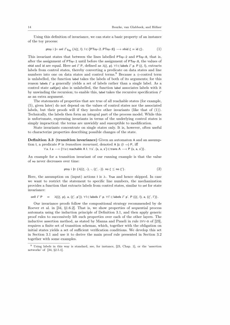
Definition 3.2 (invariance) Given an automaton A and an assumption I, a pred-icate P is (state) invariant, denoted A ||= (I →) P, iff ∀ s∈ reachable A I. P s.
We define reachability relative to an assumption on (input) actions I. When I isλ-. True, we write simply A ||= P.
14 Bourke, van Glabbeek, and Höfner
Using this definition of invariance, we can state a basic property of an instanceof the toy process:
ptoy i ||= onl ΓToy (λ(ξ, l). l∈ {PToy-:2..PToy-:8} −→ nhid ξ = id ξ) . (1)
This invariant states that between the lines labelled PToy-:2 and PToy-:8, that is,after the assignment of PToy-:1 until before the assignment of PToy-:8, the values ofnhid and id are equal. Here onl Γ P, defined as λ(ξ, p). ∀ l∈ labels Γ p. P (ξ, l), extractslabels from control states, thereby converting a predicate on data states and linenumbers into one on data states and control terms.9 Because a ⊕-control termis unlabelled, the function label takes the labels of both of its arguments; for thisreason labels Γ p generally yields a set of labels rather than a single label. As acontrol state call(pn) also is unlabelled, the function label associates labels with itby unwinding the recursion; to enable this, label takes the recursive specification Γ
as an extra argument.The statements of properties that are true of all reachable states (for example,
(5), given later) do not depend on the values of control states nor the associatedlabels, but their proofs will if they involve other invariants (like that of (1)).Technically, the labels then form an integral part of the process model. While thisis unfortunate, expressing invariants in terms of the underlying control states issimply impractical: the terms are unwieldy and susceptible to modification.
State invariants concentrate on single states only. It is, however, often usefulto characterize properties describing possible changes of the state.
Definition 3.3 (transition invariance) Given an automaton A and an assump-tion I, a predicate P is transition invariant, denoted A ||≡ (I →) P, iff
∀ a. I a −→ (∀ s∈ reachable A I. ∀ s’. (s, a, s’)∈ trans A −→ P (s, a, s’)) .
An example for a transition invariant of our running example is that the valueof no never decreases over time:
ptoy i ||≡ (λ((ξ, -), -, (ξ’, -)). no ξ ≤ no ξ’) . (2)
Here, the assumption on (input) actions I is λ-. True and hence skipped. In casewe want to restrict the statement to specific line numbers, the mechanizationprovides a function that extracts labels from control states, similar to onl for stateinvariance:
onll Γ P = λ((ξ, p), a, (ξ’, p’)). ∀ l∈ labels Γ p. ∀ l’∈ labels Γ p’. P ((ξ, l), a, (ξ’, l’)) .
Our invariance proofs follow the compositional strategy recommended by deRoever et al. in [34, §1.6.2]. That is, we show properties of sequential processautomata using the induction principle of Definition 3.1, and then apply genericproof rules to successively lift such properties over each of the other layers. Theinductive assertion method, as stated by Manna and Pnueli in rule inv-b of [23],requires a finite set of transition schemas, which, together with the obligation oninitial states yields a set of sufficient verification conditions. We develop this setin Section 3.1 and use it to derive the main proof rule presented in Section 3.2together with some examples.
9 Using labels in this way is standard, see, for instance, [23, Chap. 1], or the ‘assertionnetworks’ of [34, §2.5.1].
Mechanizing a Process Algebra for Network Protocols 15
3.1 Control terms
Given a specification Γ over finitely many process names, we can generate a finiteset of verification conditions because transitions from (’s, ’p, ’l) seqp terms alwaysyield subterms of terms in Γ . But, rather than simply considering the set of allsubterms, we prefer to define a subset of ‘control terms’ that reduces the numberof verification conditions, avoids tedious duplication in proofs, and correspondswith the obligations considered in pen-and-paper proofs. The main idea is thatthe ⊕ and call operators serve only to combine process terms: they are, in a sense,executed recursively by seqp-sos (see Section 2.1) to determine the actions that aterm offers to its environment. This is made precise by defining a relation betweensequential process terms.
Definition 3.4 (;Γ ) For a (recursive) specification Γ , let ;Γ be the smallestrelation such that (p ⊕ q) ;Γ p, (p ⊕ q) ;Γ q, and (call(pn)) ;Γ Γ pn.
We write ;Γ∗ for its reflexive transitive closure. We consider a specification to be
well formed, when the inverse of this relation is well founded:
wellformed Γ = wf {(q, p) | p ;Γ q} .10
Most of our lemmas apply only to well-formed specifications, since otherwise func-tions over the terms they contain cannot be guaranteed to terminate. Neither ofthese two specifications is well formed: Γa(1) = p ⊕ call(1); Γ b(n) = call(n+1).
We will also need a set of ‘start terms’ of a process—the subterms that can actdirectly.
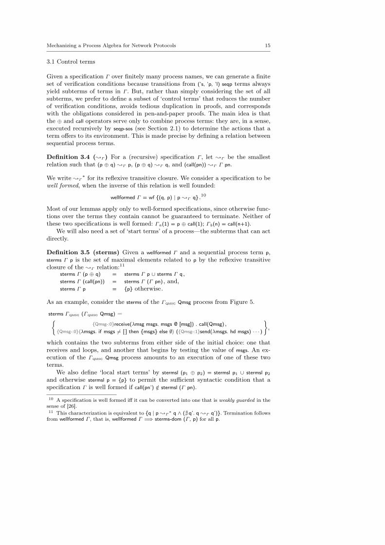
Definition 3.5 (sterms) Given a wellformed Γ and a sequential process term p,sterms Γ p is the set of maximal elements related to p by the reflexive transitiveclosure of the ;Γ relation:11
sterms Γ (p ⊕ q) = sterms Γ p ∪ sterms Γ q ,sterms Γ (call(pn)) = sterms Γ (Γ pn) , and,sterms Γ p = {p} otherwise.
As an example, consider the sterms of the Γqmsg Qmsg process from Figure 5.
sterms Γqmsg (Γqmsg Qmsg) ={{Qmsg-:0}receive(λmsg msgs. msgs @ [msg]) . call(Qmsg) ,
{Qmsg-:0}〈λmsgs. if msgs 6= [ ] then {msgs} else ∅〉 ({Qmsg-:1}send(λmsgs. hd msgs) · · · )
},
which contains the two subterms from either side of the initial choice: one thatreceives and loops, and another that begins by testing the value of msgs. An ex-ecution of the Γqmsg Qmsg process amounts to an execution of one of these twoterms.
We also define ‘local start terms’ by stermsl (p1 ⊕ p2) = stermsl p1 ∪ stermsl p2and otherwise stermsl p = {p} to permit the sufficient syntactic condition that aspecification Γ is well formed if call(pn’) /∈ stermsl (Γ pn).
10 A specification is well formed iff it can be converted into one that is weakly guarded in thesense of [26].11 This characterization is equivalent to {q | p ;Γ
∗ q ∧ (@ q’. q ;Γ q’)}. Termination followsfrom wellformed Γ , that is, wellformed Γ =⇒ sterms-dom (Γ , p) for all p.

16 Bourke, van Glabbeek, and Höfner
Since sterms Γqmsg (Γqmsg Qmsg) = stermsl (Γqmsg Qmsg), and Qmsg is the onlyprocess in Γ qmsg, we can conclude that Γ qmsg is well formed,
Similarly to the way that start terms act as direct sources of transitions, wedefine ‘derivative terms’ giving possible ‘active’ destinations of transitions.
Definition 3.6 (dterms) Given a wellformed Γ and a sequential process term p,dterms p is defined by:
dterms Γ (p ⊕ q) = dterms Γ p ∪ dterms Γ q ,dterms Γ (call(pn)) = dterms Γ (Γ pn) ,
dterms Γ ({l}〈g〉 p) = sterms Γ p ,dterms Γ ({l}[[u]] p) = sterms Γ p ,dterms Γ ({l}unicast(sid , smsg ) . p . q) = sterms Γ p ∪ sterms Γ q ,dterms Γ ({l}broadcast(smsg ) . p) = sterms Γ p ,dterms Γ ({l}groupcast(sids , smsg ) . p) = sterms Γ p ,dterms Γ ({l}send(smsg ) . p) = sterms Γ p ,dterms Γ ({l}deliver(sdata ) . p) = sterms Γ p , and,dterms Γ ({l}receive(umsg ) . p) = sterms Γ p .
For Γqmsg Qmsg, for example, we calculate dterms Γqmsg (Γqmsg Qmsg) ={Qmsg-:0}receive(λmsg msgs. msgs @ [msg]) . call(Qmsg) ,
{Qmsg-:0}〈λmsgs. if msgs 6= [ ] then {msgs} else ∅〉 ({Qmsg-:1}send(λmsgs. hd msgs) · · · ) ,{Qmsg-:1}send(λmsgs. hd msgs) . ({Qmsg-:2}[[λmsgs. tl msgs]] call(Qmsg) ⊕ · · · ) ,
{Qmsg-:1}receive(λmsg msgs. msgs @ [msg]) . call(Qmsg)
.
These derivative terms overapproximate the set of sterms of processes that can bereached in exactly one transition, since they do not consider the truth of guards(like msgs 6= [ ]) nor the willingness of communication partners (like receive(...)).
These auxiliary definitions lead to a succinct definition of the set of controlterms of a specification.
Definition 3.7 (cterms) For a specification Γ , cterms is the smallest set where:
p∈ sterms Γ (Γ pn)p∈ cterms Γ
q∈ cterms Γ p∈ dterms Γ qp∈ cterms Γ
There are, for example, six control terms in cterms Γqmsg =
{Qmsg-:0}receive(λmsg msgs. msgs @ [msg]) . call(Qmsg) ,{Qmsg-:0}〈λmsgs. if msgs 6= [ ] then {msgs} else ∅〉 ({Qmsg-:1}send(λmsgs. hd msgs) · · · ) ,
{Qmsg-:1}send(λmsgs. hd msgs) . ({Qmsg-:2}[[λmsgs. tl msgs]] call(Qmsg) ⊕ · · · ) ,{Qmsg-:2}[[λmsgs. tl msgs]] call(Qmsg) ,
{Qmsg-:2}receive(λmsg msgs. tl msgs @ [msg]) . call(Qmsg) ,{Qmsg-:1}receive(λmsg msgs. msgs @ [msg]) . call(Qmsg)
.
In terms of the main example, the set cterms ΓToy has fourteen elements; exactlyone for each printed line in Figure 3 or each transition in Figure 4.12
When proving state or transition invariants of the form onl Γ P or onll Γ P, theseare the only control states for which the conditions of Definitions 3.2 and 3.3 needbe checked.
As for sterms, it is useful to define a local version independent of any specification.
12 Of all the control terms, only those beginning with unicast may induce more than onetransition.

Mechanizing a Process Algebra for Network Protocols 17
Definition 3.8 (ctermsl) Let ctermsl be the smallest set defined by:ctermsl (p ⊕ q) = ctermsl p ∪ ctermsl q,ctermsl (call(pn)) = {call(pn)},ctermsl ({l}〈g〉 p) = {{l}〈g〉 p} ∪ ctermsl p ,ctermsl ({l}[[u]] p) = {{l}[[u]] p} ∪ ctermsl p ,ctermsl ({l}unicast(sid , smsg ) . p . q) = {{l}unicast(sid , smsg ) . p . q}
∪ (ctermsl p ∪ ctermsl q) ,ctermsl ({l}broadcast(smsg ) . p) = {{l}broadcast(smsg ) . p} ∪ ctermsl p ,ctermsl ({l}groupcast(sids , smsg ) . p) = {{l}groupcast(sids , smsg ) . p} ∪ ctermsl p ,ctermsl ({l}send(smsg ) . p) = {{l}send(smsg ) . p} ∪ ctermsl p ,ctermsl ({l}deliver(sdata ) . p) = {{l}deliver(sdata ) . p} ∪ ctermsl p , and,ctermsl ({l}receive(umsg ) . p) = {{l}receive(umsg ) . p} ∪ ctermsl p .
For our running example we have ctermsl (Γqmsg Qmsg) = cterms Γqmsg ∪ {call(Qmsg)}.Including call terms ensures that q∈ stermsl p implies q∈ ctermsl p, which facilitatesproofs. For wellformed Γ, ctermsl allows an alternative definition of cterms,
cterms Γ = {p | ∃ pn. p∈ ctermsl (Γ pn) ∧ not-call p} . (3)
While the original definition is convenient for developing the meta-theory, due tothe accompanying induction principle, this one is more useful for systematicallygenerating the set of control terms of a specification, and thus, as we will see, setsof verification conditions. And, for wellformed Γ , we have as a corollary that
cterms Γ = {p | ∃ pn. p∈ subterms (Γ pn) ∧ not-call p ∧ not-choice p} , (4)
where subterms, not-call, and not-choice are defined in the obvious way.Our example already indicates that cterms over-approximates the set of start
terms of reachable control states. Formally we have the following theorem.
Lemma 3.9 For wellformed Γ and automaton A where control-within Γ (init A) andtrans A = seqp-sos Γ , if (ξ, p)∈ reachable A I and q∈ sterms Γ p then q∈ cterms Γ .
The predicate control-within Γ Z = ∀ (ξ, p)∈Z. ∃ pn. p∈ subterms (Γ pn) serves to statethat the initial control state is within the specification.
3.2 Basic proof rule and invariants
State invariants such as (1) are solved using a procedure whose soundness is jus-tified as a theorem. The proof exploits (3) and Lemma 3.9.
Theorem 3.10 To prove A ||= (I →) onl Γ P, where wellformed Γ , simple-labels Γ ,control-within Γ (init A), and trans A = seqp-sos Γ , it suffices
(init) for arbitrary (ξ, p)∈ init A and l∈ labels Γ p, to show P (ξ, l), and,(trans) for arbitrary p∈ ctermsl (Γ pn), but not-call p, and l∈ labels Γ p, given that
p∈ sterms Γ pp for some (ξ, pp)∈ reachable A I, to assume P (ξ, l), and thenfor any a with I a and any (ξ’, q) such that ((ξ, p), a, (ξ’, q))∈ seqp-sos Γ andl’∈ labels Γ q, to show P (ξ’, l’).
18 Bourke, van Glabbeek, and Höfner
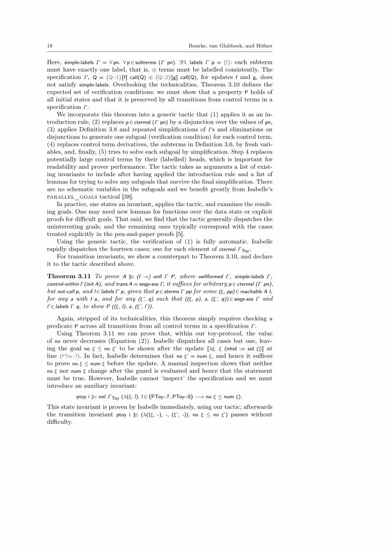
Here, simple-labels Γ = ∀ pn. ∀ p∈ subterms (Γ pn). ∃! l. labels Γ p = {l}: each subtermmust have exactly one label, that is, ⊕ terms must be labelled consistently. Thespecification Γ c Q = {Q-:1}[[f]] call(Q) ⊕ {Q-:2}[[g]] call(Q), for updates f and g, doesnot satisfy simple-labels. Overlooking the technicalities, Theorem 3.10 defines theexpected set of verification conditions: we must show that a property P holds ofall initial states and that it is preserved by all transitions from control terms in aspecification Γ .
We incorporate this theorem into a generic tactic that (1) applies it as an in-troduction rule, (2) replaces p∈ ctermsl (Γ pn) by a disjunction over the values of pn,(3) applies Definition 3.8 and repeated simplifications of Γ s and eliminations ondisjunctions to generate one subgoal (verification condition) for each control term,(4) replaces control term derivatives, the subterms in Definition 3.6, by fresh vari-ables, and, finally, (5) tries to solve each subgoal by simplification. Step 4 replacespotentially large control terms by their (labelled) heads, which is important forreadability and prover performance. The tactic takes as arguments a list of exist-ing invariants to include after having applied the introduction rule and a list oflemmas for trying to solve any subgoals that survive the final simplification. Thereare no schematic variables in the subgoals and we benefit greatly from Isabelle’sparallel_goals tactical [38].
In practice, one states an invariant, applies the tactic, and examines the result-ing goals. One may need new lemmas for functions over the data state or explicitproofs for difficult goals. That said, we find that the tactic generally dispatches theuninteresting goals, and the remaining ones typically correspond with the casestreated explicitly in the pen-and-paper proofs [5].
Using the generic tactic, the verification of (1) is fully automatic. Isabellerapidly dispatches the fourteen cases; one for each element of ctermsl ΓToy.
For transition invariants, we show a counterpart to Theorem 3.10, and declareit to the tactic described above.
Theorem 3.11 To prove A ||≡ (I →) onll Γ P, where wellformed Γ , simple-labels Γ ,control-withinΓ (init A), and trans A = seqp-sos Γ, it suffices for arbitrary p∈ ctermsl (Γ pn),but not-call p, and l∈ labels Γ p, given that p∈ sterms Γ pp for some (ξ, pp)∈ reachable A I,for any a with I a, and for any (ξ’, q) such that ((ξ, p), a, (ξ’, q))∈ seqp-sos Γ andl’∈ labels Γ q, to show P ((ξ, l), a, (ξ’, l’)).
Again, stripped of its technicalities, this theorem simply requires checking apredicate P across all transitions from all control terms in a specification Γ .
Using Theorem 3.11 we can prove that, within our toy-protocol, the valueof no never decreases (Equation (2)). Isabelle dispatches all cases but one, leav-ing the goal no ξ ≤ no ξ’ to be shown after the update [[λξ. ξ (|nhid := sid ξ|)]] atline {PToy-:7}. In fact, Isabelle determines that no ξ’ = num ξ, and hence it sufficesto prove no ξ ≤ num ξ before the update. A manual inspection shows that neitherno ξ nor num ξ change after the guard is evaluated and hence that the statementmust be true. However, Isabelle cannot ‘inspect’ the specification and we mustintroduce an auxiliary invariant:
ptoy i ||= onl ΓToy (λ(ξ, l). l∈ {PToy-:7..PToy-:8} −→ no ξ ≤ num ξ) .
This state invariant is proven by Isabelle immediately, using our tactic; afterwardsthe transition invariant ptoy i ||≡ (λ((ξ, -), -, (ξ’, -)). no ξ ≤ no ξ’) passes withoutdifficulty.

Mechanizing a Process Algebra for Network Protocols 19
4 Open invariance
The analysis of network protocols often requires ‘inter-node’ invariants, like
wf-net-tree Ψ =⇒ closed (pnet (λi. ptoy i 〈〈 qmsg) Ψ) ||=
netglobal (λσ. ∀ i. no (σ i) ≤ no (σ (nhid (σ i)))) , (5)
which states that, for any network topology, specified as a net-tree with disjointnode addresses (wf-net-tree Ψ), the value of no at a node is never greater than itsvalue at the ‘next hop’—the address in nhid. This is a property of a global state σmapping addresses to corresponding local data states ξ.
We build a global state in two steps. The first step maps a tree of states to apartial function from addresses to the data states of node processes:
netlift ps (s iR) = [i 7→ fst (ps s)] ,
netlift ps (s q t) = netlift ps s ++ netlift ps t .
The netlift function is parameterized by a ‘process selection’ function ps that isapplied to the state of a node process—that is, a state of the np i of Section 2.4.In typical applications, such a state is the local parallel composition of a protocolprocess and a message queue (see Section 2.2). In such a case, ps selects just theprotocol process, while abstracting from the queue. The first netlift rule associatesthe node address i with the process data state. The fst elides the local componentof the process state. The second rule concatenates the partial maps generated foreach branch of the state tree. The assumption of disjoint node addresses is criticalfor reasoning about the resulting map.
The idea is to treat all (local) data states ξ as a single global state σ and toabstract from local details like the process control state and queue. The local detailsare important for stating and showing intermediate lemmas, but their inclusion inglobal invariants would be an unnecessary complication.
The second step in building the global state is to add default elements df forundefined addresses i. We first define the auxiliary function
default df f = (λi. case f i of None ⇒ df i | Some s ⇒ s) ,
and then apply it to the result of netlift in the definition of netglobal. For our examplewe set
netglobal P = λs. P (default toy-init (netlift fst s)) .
Basically, we associate a state with every node address by setting the state atnon-existent addresses to the initial state (here toy-init). The advantage is thatinvariants and associated proofs need not consider the possibility of an undefinedstate or, in other words, that σ i could be None. In (5), for example, this conventionavoids three guards on address definedness. One must decide, however, whetherthis convention is appropriate for a given property.
While we can readily state inter-node invariants of a complete model, showingthem compositionally is another issue. Sections 4.1 and 4.2 present a way to stateand prove such invariants at the level of sequential processes—in our example thatis, with only ptoy i left of the turnstile. Sections 4.3 and 4.4 present, respectively,rules for lifting such results to network models and for recovering invariants like (5).
20 Bourke, van Glabbeek, and Höfner
σ’ i = u (σ i)((σ, {l}[[u]] p), τ , (σ’, p))∈ oseqp-sos Γ i
σ’ i∈ g (σ i)((σ, {l}〈g〉 p), τ , (σ’, p))∈ oseqp-sos Γ i
σ’ i = σ i((σ, {l}unicast(sid , smsg ) . p . q), unicast (sid (σ i)) (smsg (σ i)), (σ’, p))∈ oseqp-sos Γ i
σ’ i = σ i((σ, {l}unicast(sid , smsg ) . p . q), ¬unicast (sid (σ i)), (σ’, q))∈ oseqp-sos Γ i
σ’ i = σ i((σ, {l}broadcast(smsg ) . p), broadcast (smsg (σ i)), (σ’, p))∈ oseqp-sos Γ i
σ’ i = σ i((σ, {l}groupcast(sids , smsg ) . p), groupcast (sids (σ i)) (smsg (σ i)), (σ’, p))∈ oseqp-sos Γ i
σ’ i = σ i((σ, {l}send(smsg ) . p), send (smsg (σ i)), (σ’, p))∈ oseqp-sos Γ i
σ’ i = umsg msg (σ i)((σ, {l}receive(umsg ) . p), receive msg, (σ’, p))∈ oseqp-sos Γ i
σ’ i = σ i((σ, {l}deliver(sdata ) . p), deliver (sdata (σ i)), (σ’, p))∈ oseqp-sos Γ i
((σ, p), a, (σ’, p’))∈ oseqp-sos Γ i((σ, p ⊕ q), a, (σ’, p’))∈ oseqp-sos Γ i
((σ, q), a, (σ’, q’))∈ oseqp-sos Γ i((σ, p ⊕ q), a, (σ’, q’))∈ oseqp-sos Γ i
((σ, Γ pn), a, (σ’, p’))∈ oseqp-sos Γ i((σ, call(pn)), a, (σ’, p’))∈ oseqp-sos Γ i
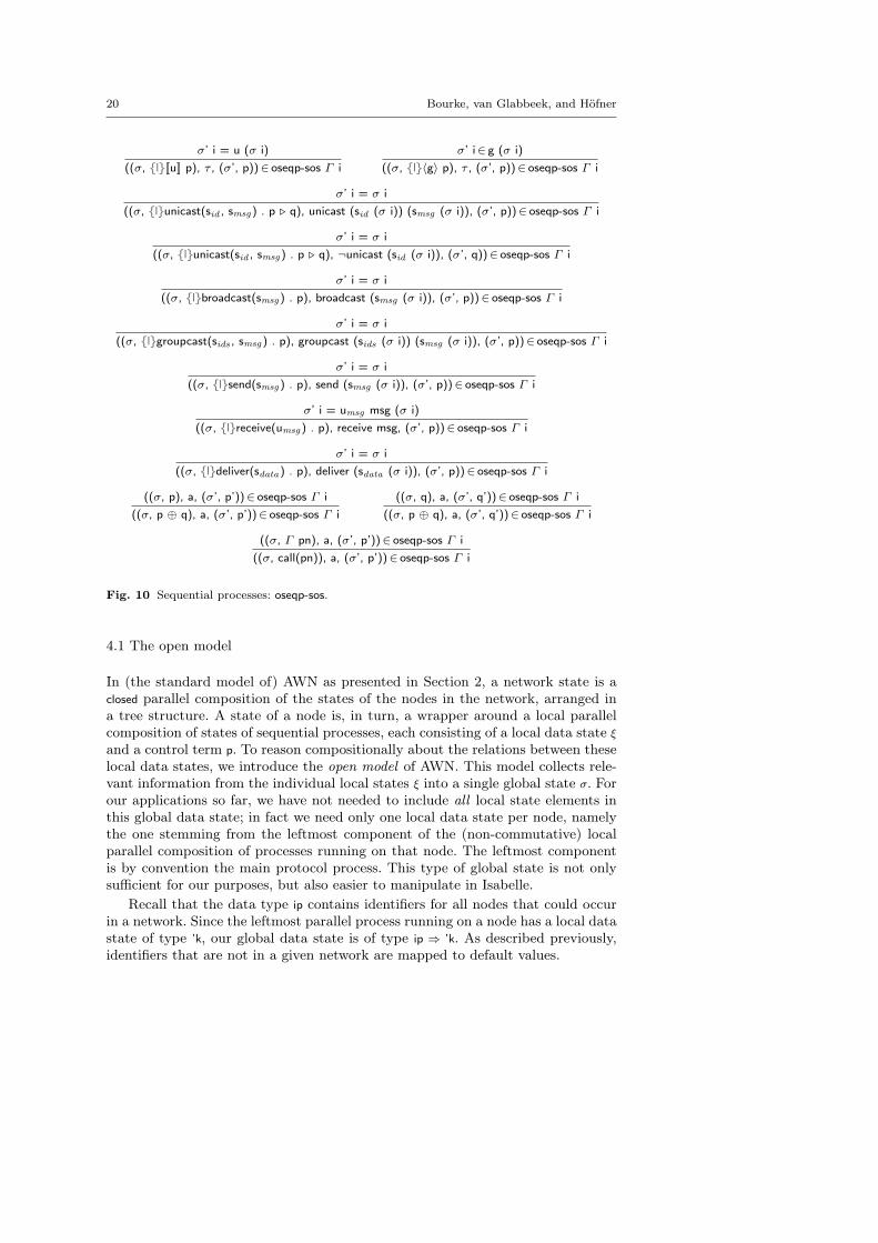
Fig. 10 Sequential processes: oseqp-sos.
4.1 The open model
In (the standard model of) AWN as presented in Section 2, a network state is aclosed parallel composition of the states of the nodes in the network, arranged ina tree structure. A state of a node is, in turn, a wrapper around a local parallelcomposition of states of sequential processes, each consisting of a local data state ξand a control term p. To reason compositionally about the relations between theselocal data states, we introduce the open model of AWN. This model collects rele-vant information from the individual local states ξ into a single global state σ. Forour applications so far, we have not needed to include all local state elements inthis global data state; in fact we need only one local data state per node, namelythe one stemming from the leftmost component of the (non-commutative) localparallel composition of processes running on that node. The leftmost componentis by convention the main protocol process. This type of global state is not onlysufficient for our purposes, but also easier to manipulate in Isabelle.
Recall that the data type ip contains identifiers for all nodes that could occurin a network. Since the leftmost parallel process running on a node has a local datastate of type ’k, our global data state is of type ip ⇒ ’k. As described previously,identifiers that are not in a given network are mapped to default values.

Mechanizing a Process Algebra for Network Protocols 21
((σ, s), a, (σ’, s’))∈TA∧m. a 6= receive m
((σ, (s, t)), a, (σ’, (s’, t)))∈ oparp-sos i TA TB
(t, a, t’)∈TB∧m. a 6= send m σ’ i = σ i
((σ, (s, t)), a, (σ’, (s, t’)))∈ oparp-sos i TA TB
((σ, s), receive m, (σ’, s’))∈TA (t, send m, t’)∈TB
((σ, (s, t)), τ , (σ’, (s’, t’)))∈ oparp-sos i TA TB
Fig. 11 Parallel processes: oparp-sos.
In the open model, a state of a network is described as a pair (σ, s) of such aglobal state and a closed parallel composition s of the control states of the nodesin the network. The control state of a node is a wrapper around a local parallelcomposition of states of sequential processes, where we take only the control term pfrom the state (ξ, p) of the leftmost parallel process running on the node, and theentire state from all other components. As a result, a state in the open modelcontains exactly the same information as a state in the default model, even if it isarranged differently.
Figures 10–14 present the SOS rules for the open model. Many of them aresimilar to the rules presented in Section 2; for the sake of completeness we listthem nevertheless.
4.1.1 Sequential Processes
The rules for the sequential control terms in the open model, oseqp-sos, are presentedin Figure 10. They are nearly identical to the ones in the original model, but have tobe parameterized by an address i and constrain only that entry of the global state,either to say how it changes (σ’ i = u (σ i)) or that it does not change (σ’ i = σ i).These rules do not restrict changes in the data state of any other node j (j 6=i).In principle, the data states of these nodes can change arbitrarily, so that anystate (σ, p) has infinitely many outgoing transitions. However, the compositionwith other nodes, introduced in a higher layer of the process algebra, will limit theset of outgoing transitions by combining the restrictions imposed by each of thenodes.
4.1.2 Local parallel composition
The states (σ, s) in an automaton of the open model are of type (ip ⇒ ’k) × ’s withip ⇒ ’k the type of global data states and ’s the type of control states. Hence, suchan automaton has type ((ip ⇒ ’k) × ’s, ’a) automaton. The local parallel compositionof the open model pairs an open automaton with a standard one, and thus has type((ip ⇒ ’k) × ’s, ’a) automaton ⇒ (’t, ’a) automaton ⇒ ((ip ⇒ ’k) × (’s × ’t), ’a) automaton.
The rules for oparp-sos, depicted in Figure 11, only allow the first sub-processto constrain σ: the global data state that appears in the parallel composition issimply taken from its first component. This choice precludes comparing the statesof qmsgs (and any other local filters) across a network, but it also simplifies themechanics and use of this layer of the framework. Since our mechanization aims at

22 Bourke, van Glabbeek, and Höfner
((σ, s), unicast dst m, (σ’, s’))∈TA dst∈R((σ, s i
R), {dst}:∗cast(m), (σ’, s’ iR))∈ onode-sos TA
((σ, s), ¬unicast dst, (σ’, s’))∈TA dst /∈ R ∀ j. j 6= i −→ σ’ j = σ j((σ, s i
R), τ , (σ’, s’iR))∈ onode-sos TA
((σ, s), broadcast m, (σ’, s’))∈TA
((σ, s iR), R:∗cast(m), (σ’, s’ iR))∈ onode-sos TA
((σ, s), groupcast D m, (σ’, s’))∈TA
((σ, s iR), (R ∩ D):∗cast(m), (σ’, s’ iR))∈ onode-sos TA
((σ, s), receive m, (σ’, s’))∈TA
((σ, s iR), {i}¬∅:arrive(m), (σ’, s’ iR))∈ onode-sos TA
((σ, s), deliver d, (σ’, s’))∈TA ∀ j. j 6= i −→ σ’ j = σ j((σ, s i
R), i:deliver(d), (σ’, s’iR))∈ onode-sos TA
((σ, s), τ , (σ’, s’))∈TA ∀ j 6= i. σ’ j = σ j((σ, s i
R), τ , (σ’, s’iR))∈ onode-sos TA
σ’ i = σ i((σ, s i
R), ∅¬{i}:arrive(m), (σ’, s iR))∈ onode-sos TA
σ’ i = σ i((σ, s i
R), connect(i, i’), (σ’, siR ∪ {i’}))∈ onode-sos TA
σ’ i = σ i((σ, s i
R), connect(i’, i), (σ’, siR ∪ {i’}))∈ onode-sos TA
σ’ i = σ i((σ, s i
R), disconnect(i, i’), (σ’, siR - {i’}))∈ onode-sos TA
σ’ i = σ i((σ, s i
R), disconnect(i’, i), (σ’, siR - {i’}))∈ onode-sos TA
i 6= i’ i 6= i’’ σ’ i = σ i((σ, s i
R), connect(i’, i’’), (σ’, siR))∈ onode-sos TA
i 6= i’ i 6= i’’ σ’ i = σ i((σ, s i
R), disconnect(i’, i’’), (σ’, siR))∈ onode-sos TA
Fig. 12 Nodes: onode-sos.
the verification of (routing) protocols [5], which nearly always implement a queue,simplifying the mechanization in this way seems reasonable. The treatment of theother layers is independent of this choice. So, if our work were to be applied inanother setting where queues are not used, or where data states of more than oneparallel control term need to be lifted to a control state, only this layer need beadapted.
Mechanizing a Process Algebra for Network Protocols 23
((σ, s), R:∗cast(m), (σ’, s’))∈TA
((σ, t), H¬K:arrive(m), (σ’, t’))∈TB H ⊆ R K ∩ R = ∅((σ, s q t), R:∗cast(m), (σ’, s’ q t’))∈ opnet-sos TA TB
((σ, s), H¬K:arrive(m), (σ’, s’))∈TA
((σ, t), R:∗cast(m), (σ’, t’))∈TB H ⊆ R K ∩ R = ∅((σ, s q t), R:∗cast(m), (σ’, s’ q t’))∈ opnet-sos TA TB
((σ, s), H¬K:arrive(m), (σ’, s’))∈TA ((σ, t), H’¬K’:arrive(m), (σ’, t’))∈TB
((σ, s q t), (H ∪ H’)¬(K ∪ K’):arrive(m), (σ’, s’ q t’))∈ opnet-sos TA TB
((σ, s), i:deliver(d), (σ’, s’))∈TA
((σ, s q t), i:deliver(d), (σ’, s’ q t))∈ opnet-sos TA TB
((σ, t), i:deliver(d), (σ’, t’))∈TB
((σ, s q t), i:deliver(d), (σ’, s q t’))∈ opnet-sos TA TB
((σ, s), τ , (σ’, s’))∈TA
((σ, s q t), τ , (σ’, s’ q t))∈ opnet-sos TA TB
((σ, t), τ , (σ’, t’))∈TB
((σ, s q t), τ , (σ’, s q t’))∈ opnet-sos TA TB
((σ, s), connect(i, i’), (σ’, s’))∈TA ((σ, t), connect(i, i’), (σ’, t’))∈TB
((σ, s q t), connect(i, i’), (σ’, s’ q t’))∈ opnet-sos TA TB
((σ, s), disconnect(i, i’), (σ’, s’))∈TA ((σ, t), disconnect(i, i’), (σ’, t’))∈TB
((σ, s q t), disconnect(i, i’), (σ’, s’ q t’))∈ opnet-sos TA TB
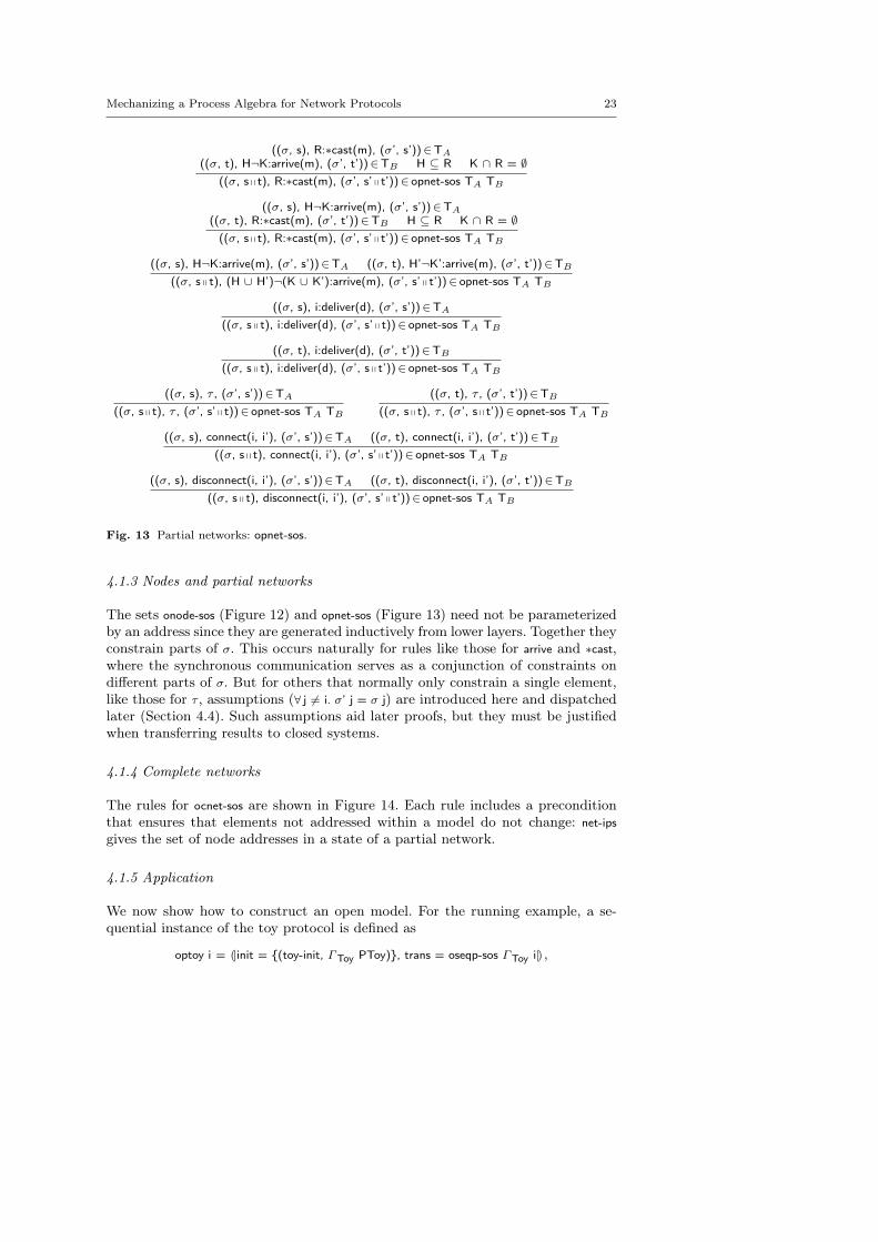
Fig. 13 Partial networks: opnet-sos.
4.1.3 Nodes and partial networks
The sets onode-sos (Figure 12) and opnet-sos (Figure 13) need not be parameterizedby an address since they are generated inductively from lower layers. Together theyconstrain parts of σ. This occurs naturally for rules like those for arrive and ∗cast,where the synchronous communication serves as a conjunction of constraints ondifferent parts of σ. But for others that normally only constrain a single element,like those for τ , assumptions (∀ j 6= i. σ’ j = σ j) are introduced here and dispatchedlater (Section 4.4). Such assumptions aid later proofs, but they must be justifiedwhen transferring results to closed systems.
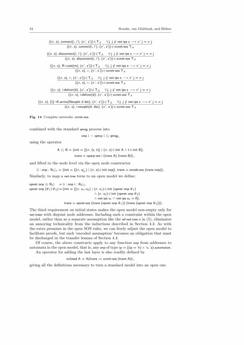
4.1.4 Complete networks
The rules for ocnet-sos are shown in Figure 14. Each rule includes a preconditionthat ensures that elements not addressed within a model do not change: net-ipsgives the set of node addresses in a state of a partial network.
4.1.5 Application
We now show how to construct an open model. For the running example, a se-quential instance of the toy protocol is defined as
optoy i = (|init = {(toy-init, ΓToy PToy)}, trans = oseqp-sos ΓToy i|) ,
24 Bourke, van Glabbeek, and Höfner
((σ, s), connect(i, i’), (σ’, s’))∈TA ∀ j. j /∈ net-ips s −→ σ’ j = σ j((σ, s), connect(i, i’), (σ’, s’))∈ ocnet-sos TA
((σ, s), disconnect(i, i’), (σ’, s’))∈TA ∀ j. j /∈ net-ips s −→ σ’ j = σ j((σ, s), disconnect(i, i’), (σ’, s’))∈ ocnet-sos TA
((σ, s), R:∗cast(m), (σ’, s’))∈TA ∀ j. j /∈ net-ips s −→ σ’ j = σ j((σ, s), τ , (σ’, s’))∈ ocnet-sos TA
((σ, s), τ , (σ’, s’))∈TA ∀ j. j /∈ net-ips s −→ σ’ j = σ j((σ, s), τ , (σ’, s’))∈ ocnet-sos TA
((σ, s), i:deliver(d), (σ’, s’))∈TA ∀ j. j /∈ net-ips s −→ σ’ j = σ j((σ, s), i:deliver(d), (σ’, s’))∈ ocnet-sos TA
((σ, s), {i}¬K:arrive(Newpkt d dst), (σ’, s’))∈TA ∀ j. j /∈ net-ips s −→ σ’ j = σ j((σ, s), i:newpkt(d, dst), (σ’, s’))∈ ocnet-sos TA
Fig. 14 Complete networks: ocnet-sos.
combined with the standard qmsg process into
onp i = optoy i 〈〈i qmsg ,
using the operator
A 〈〈i B = (|init = {(σ, (s, t)) | (σ, s)∈ init A ∧ t∈ init B},
trans = oparp-sos i (trans A) (trans B)|) ,
and lifted to the node level via the open node constructor
〈i : onp : R0〉o = (|init = {(σ, s iR0) | (σ, s)∈ init onp}, trans = onode-sos (trans onp)|) .
Similarly, to map a net-tree term to an open model we define:
opnet onp 〈i; R0〉 = 〈i : onp i : R0〉oopnet onp (Ψ1‖Ψ2) = (|init = {(σ, s1q s2) | (σ, s1)∈ init (opnet onp Ψ1)
∧ (σ, s2)∈ init (opnet onp Ψ2)∧ net-ips s1 ∩ net-ips s2 = ∅},
trans = opnet-sos (trans (opnet onp Ψ1)) (trans (opnet onp Ψ2))|) .
The third requirement on initial states makes the open model non-empty only fornet-trees with disjoint node addresses. Including such a constraint within the openmodel, rather than as a separate assumption like the wf-net-tree n in (5), eliminatesan annoying technicality from the inductions described in Section 4.3. As withthe extra premises in the open SOS rules, we can freely adjust the open model tofacilitate proofs, but each ‘encoded assumption’ becomes an obligation that mustbe discharged in the transfer lemma of Section 4.4.
Of course, the above constructs apply to any function onp from addresses toautomata in the open model, that is, any onp of type ip⇒ ((ip⇒ ’k) × ’s, ’a) automaton.
An operator for adding the last layer is also readily defined by
oclosed A = A(|trans := ocnet-sos (trans A)|) ,
giving all the definitions necessary to turn a standard model into an open one.
Mechanizing a Process Algebra for Network Protocols 25
4.2 Open invariants
The basic definitions of reachability, invariance, and transition invariance, Defi-nitions 3.1–3.3, apply to open models since they are given for generic automata,but constructing a compositional proof requires considering the effects of bothsynchronized and interleaved actions of possible environments. Our automaton Acould, for instance, be a partial network, consisting of several nodes, and the envi-ronment could be another partial network running in parallel. An action performedby the environment and the automaton together, or indeed, since the distinction isunimportant here, by the automaton alone, is termed synchronized and an actionmade by the environment without the participation of the automaton is termedinterleaved. We identify the nature of a synchronized action by the environmentthrough the action of A that synchronizes with it. We focus first of all on the casewhere A is a single node i.
The proper analysis of properties of A, such as (5), often requires assumptionson the behaviour of the environment. We consider assumptions on both synchro-nized and interleaved actions.
A typical example for an assumption on synchronized actions is
(∀ j. j 6= i −→ no (σ j) ≤ no (σ’ j)) ∧ orecvmsg msg-ok σ a , (6)
where orecvmsg applies a predicate (here msg-ok) to receive actions and is otherwisetrue: msg-ok σ (Pkt data src) = (data ≤ no (σ src)) and msg-ok σ (Newpkt d dst) = True. So,the assumption manifests two properties of the environment (nodes that are notequal to i) (1) it guarantees that all nodes different from i preserve the propertythat the value of no cannot be decreased by the protocol; (2) whenever a Pktmessage is sent, the value d stored in the message is smaller than or equal to thecurrent value of no, stored at the sender of the message src. The synchronizationoccurs via the exchange of messages.
A typical example for an interleaved (un-synchronized) action from the envi-ronment is
(∀ j. j 6= i −→ no (σ j) ≤ no (σ’ j)) ∧ σ’ i = σ i , (7)
This assumption states that (1) nodes that are not equal to i do not decrease thevalue of no—as before—and (2) that the data state at node i does not change. Sotransitions of the environment may interleave with actions performed by node i,as long as they are ‘well-behaved’ and do not interfere with the state of i.
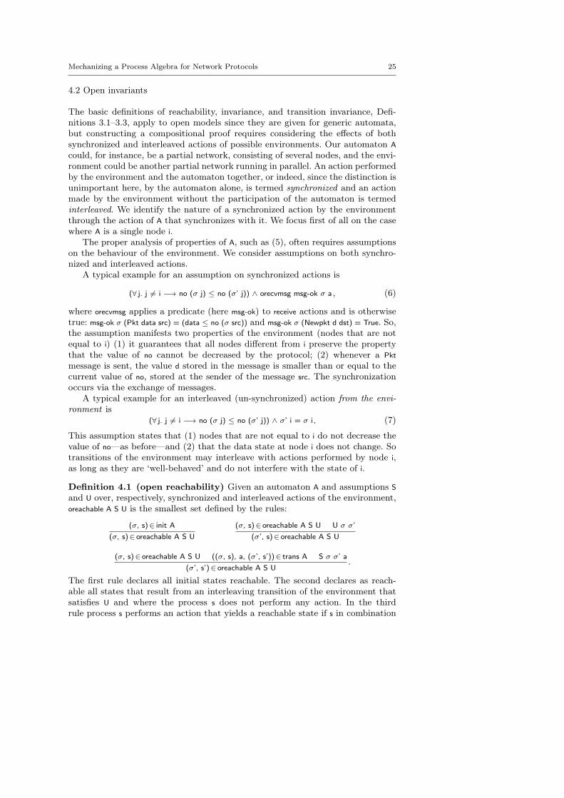
Definition 4.1 (open reachability) Given an automaton A and assumptions Sand U over, respectively, synchronized and interleaved actions of the environment,oreachable A S U is the smallest set defined by the rules:
(σ, s)∈ init A(σ, s)∈ oreachable A S U
(σ, s)∈ oreachable A S U U σ σ’(σ’, s)∈ oreachable A S U
(σ, s)∈ oreachable A S U ((σ, s), a, (σ’, s’))∈ trans A S σ σ’ a(σ’, s’)∈ oreachable A S U
.
The first rule declares all initial states reachable. The second declares as reach-able all states that result from an interleaving transition of the environment thatsatisfies U and where the process s does not perform any action. In the thirdrule process s performs an action that yields a reachable state if s in combination
26 Bourke, van Glabbeek, and Höfner
σ, s σ’, s’ σ’’, s’a
S σ σ’ a U σ’ σ”
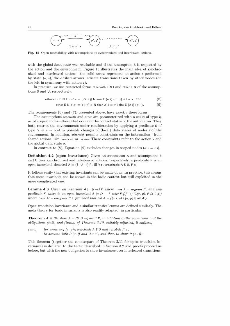
Fig. 15 Open reachability with assumptions on synchronized and interleaved actions.
with the global data state was reachable and if the assumption S is respected bythe action and the environment. Figure 15 illustrates the main idea of synchro-nized and interleaved actions—the solid arrow represents an action a performedby state (σ, s), the dashed arrows indicate transitions taken by other nodes (onthe left in synchrony with action a).
In practice, we use restricted forms otherwith E N I and other E N of the assump-tions S and U, respectively:
otherwith E N I σ σ’ a = (∀ i. i /∈ N −→ E (σ i) (σ’ i)) ∧ I σ a , and (8)other E N σ σ’ = ∀ i. if i∈N then σ’ i = σ i else E (σ i) (σ’ i) . (9)
The requirements (6) and (7), presented above, have exactly these forms.The assumptions otherwith and other are parameterized with a set N of type ip
set of scoped nodes—those that occur in the control states of the automaton. Theyboth restrict the environments under consideration by applying a predicate E oftype ’s ⇒ ’s ⇒ bool to possible changes of (local) data states of nodes i of theenvironment. In addition, otherwith permits constraints on the information I fromshared actions, like broadcast or receive. These constraints refer to the action a andthe global data state σ.
In contrast to (8), Equation (9) excludes changes in scoped nodes (σ’ i = σ i).
Definition 4.2 (open invariance) Given an automaton A and assumptions Sand U over synchronized and interleaved actions, respectively, a predicate P is anopen invariant, denoted A |= (S, U →) P, iff ∀ s∈ oreachable A S U. P s.
It follows easily that existing invariants can be made open. In practice, this meansthat most invariants can be shown in the basic context but still exploited in themore complicated one.
Lemma 4.3 Given an invariant A ||= (I →) P where trans A = seqp-sos Γ , and anypredicate F, there is an open invariant A’ |= (λ- -. I, other F {i} →) (λ(σ, p). P (σ i, p))where trans A’ = oseqp-sos Γ i, provided that init A = {(σ i, p) | (σ, p)∈ init A’}.
Open transition invariance and a similar transfer lemma are defined similarly. Themeta theory for basic invariants is also readily adapted, in particular,
Theorem 4.4 To show A |= (S, U→) onl Γ P, in addition to the conditions and theobligations (init) and (trans) of Theorem 3.10, suitably adjusted, it suffices,
(env) for arbitrary (σ, p)∈ oreachable A S U and l∈ labels Γ p ,to assume both P (σ, l) and U σ σ’, and then to show P (σ’, l) .
This theorem (together the counterpart of Theorem 3.11 for open transition in-variance) is declared to the tactic described in Section 3.2 and proofs proceed asbefore, but with the new obligation to show invariance over interleaved transitions.
Mechanizing a Process Algebra for Network Protocols 27
cnet-sos ocnet-sos
pnet-sos opnet-sos
node-sos onode-sos
parp-sos oparp-sos
seqp-sos oseqp-sos
closed (pnet (λi. ptoy i 〈〈 qmsg) Ψ) ||= P
ptoy i ||= P1 optoy i |= P ′1
optoy i 〈〈 qmsg |= P ′2
〈i : optoy i 〈〈 qmsg : R0〉o |= P ′3
opnet (λi. optoy i 〈〈 qmsg) Ψ |= P ′4
oclosed (opnet (λi. optoy i 〈〈 qmsg) Ψ) |= P ′5
Corollary 4.8(qmsg lifting)
Corollary 4.10(onode lifting)
Corollary 4.12(opnet lifting)
Corollary 4.14(ocnet lifting)
Corollary 4.16 (transfer)
Lemma 4.3 (‘open’ invariant)
Theorem 3.10invariance proof
Theorem 4.4open invariance proof
Fig. 16 Schema of the overall proof structure.
We finally have sufficient machinery to state and prove Invariant (5) at thelevel of a sequential process:
optoy i |= (otherwith nos-inc {i} (orecvmsg msg-ok), other nos-inc {i} →)(λ(σ, -). no (σ i) ≤ no (σ (nhid (σ i)))) , (10)
where nos-inc ξ ξ’ = no ξ ≤ no ξ’, So, given that the variables no in the environmentnever decrease and that incoming Pkts reflect the state of the sender, there is arelation between the local node and the next hop. Similar invariants occur in proofsof realistic protocols [5].
4.3 Lifting open invariants
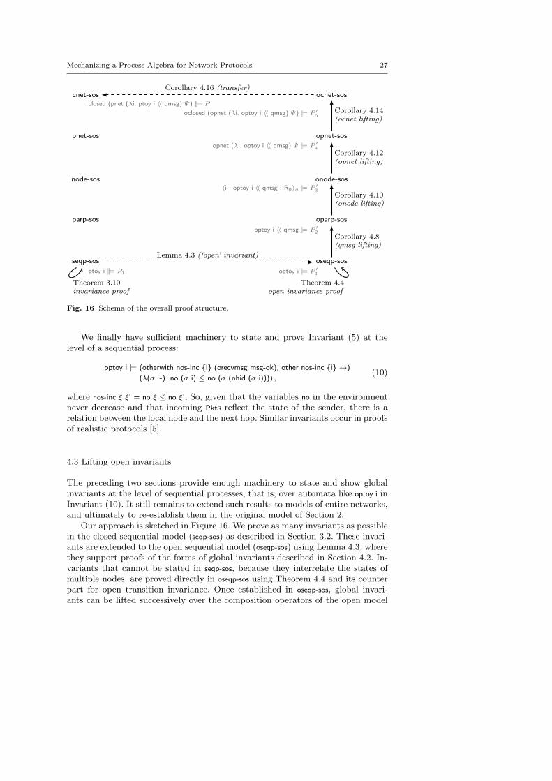
The preceding two sections provide enough machinery to state and show globalinvariants at the level of sequential processes, that is, over automata like optoy i inInvariant (10). It still remains to extend such results to models of entire networks,and ultimately to re-establish them in the original model of Section 2.
Our approach is sketched in Figure 16. We prove as many invariants as possiblein the closed sequential model (seqp-sos) as described in Section 3.2. These invari-ants are extended to the open sequential model (oseqp-sos) using Lemma 4.3, wherethey support proofs of the forms of global invariants described in Section 4.2. In-variants that cannot be stated in seqp-sos, because they interrelate the states ofmultiple nodes, are proved directly in oseqp-sos using Theorem 4.4 and its counterpart for open transition invariance. Once established in oseqp-sos, global invari-ants can be lifted successively over the composition operators of the open model
28 Bourke, van Glabbeek, and Höfner
(oparp-sos, onode-sos, opnet-sos, ocnet-sos), using the lemmas described in this section,and then transferred into the closed complete model (cnet-sos), using the lemmadescribed in the next section. Figure 16 shows, in grey, examples of the forms ofinvariants at each stage. The goal is to show a property P over an entire arbitrarynetwork in the closed model (at top-left). The property P is proven via a succes-sion of intermediate invariants, starting with P1, which is expressed relative to asingle node, possibly in relation to the rest of the network (P ′1). At each step itsform changes slightly (P ′2, P ′3, P ′4, and P ′5) to hide technical details introduced ateach layer and as its range extends to multiple nodes.
The first lifting rule (Corollary 4.8) treats composition with the qmsg process.It mixes oreachable and reachable predicates: the former for the automaton beinglifted, the latter for properties of qmsg. Two main properties of qmsg are required:only received messages are added to the queue and sent messages come from thequeue. They are shown using the techniques of Section 3.
Lemma 4.5 qmsg ||≡ (λ((msgs, q), a, (msgs’, q’)).case a of receive m ⇒ set msgs’ ⊆ set (msgs @ [m])
| - ⇒ set msgs’ ⊆ set msgs) .
Lemma 4.6 qmsg ||≡ (λ((msgs, q), a, -). sendmsg (λm. m∈ set msgs) a) .
These two properties of qmsg are used to prove a lemma that decomposes openreachability of A 〈〈i qmsg into open reachability of A and reachability of qmsg.
Lemma 4.7 (qmsg reachability)Given (σ, (s, (msgs, q)))∈ oreachable (A 〈〈i qmsg) S U, with assumptions on synchronizingand interleaved transitions S = otherwith E {i} (orecvmsg M) and U = other F {i}, andprovided
1. F is reflexive,2. for all ξ, ξ’, E ξ ξ’ implies F ξ ξ’,3. A |≡ (S, U →) (λ((σ, -), -, (σ’, -)). F (σ i) (σ’ i)), and,4. for all σ, σ’, m, ∀ j. F (σ j) (σ’ j) and M σ m imply M σ’ m,
then (σ, s)∈ oreachable A S U and (msgs, q)∈ reachable qmsg (recvmsg (M σ)), and further-more ∀m∈ set msgs. M σ m.
In the qmsg part of the local state (msgs, q), msgs is a list of messages and q is thecontrol state of the queue. We write set msgs to generate a set of messages from thelist of messages. The key intuition behind the four clauses is that every message mreceived, queued, and sent by qmsg must satisfy M σ m. That is, the propertiesof messages received into the queue continue to hold—even as the environmentand thus the original senders act—until those messages are transmitted from thequeue to the automaton A. The proof is by induction over oreachable. The M’s arepreserved when the external environment acts independently (1, 4), when it actssynchronously (2, 4), and when the local process acts (3, 4).
The preceding lemma allows open reachability of the parallel composition tobe decomposed into (open) reachability of its components. It follows easily that aninvariant of the principle component (A) is also an invariant of the composition.

Mechanizing a Process Algebra for Network Protocols 29
Corollary 4.8 (qmsg lifting) Given A |= (S, U→) (λ(σ, -). P σ), with the predicatesS = otherwith E {i} (orecvmsg M) and U = other F {i}, and provided
1. F is reflexive,2. for all ξ, ξ’, E ξ ξ’ implies F ξ ξ’,3. A |≡ (S, U →) (λ((σ, -), -, (σ’, -)). F (σ i) (σ’ i)) , and,4. for all σ, σ’, m, ∀ j. F (σ j) (σ’ j) and M σ m imply M σ’ m,
then A 〈〈i qmsg |= (S, U →) (λ(σ, -). P σ).
This lifting rule is specific to the queue model presented in Figure 5. Changes tothe model may necessitate changes to the rule or its proof, or indeed, a differentparallel composition would require a new rule and proof. No assumptions are made,however, on the structure of A, the automaton being lifted.
The rule for lifting to the node level is straightforward since a node simplyencapsulates the state of the underlying model. It is necessary, though, to adaptassumptions on receive actions (orecvmsg) to arrive actions (oarrivemsg), but this isessentially a minor technicality.
Lemma 4.9 (onode reachability) If, for all ξ and ξ’, E ξ ξ’ implies F ξ ξ’, thengiven (σ, s i
R)∈ oreachable (〈i : A : R0〉o) (otherwith E {i} (oarrivemsg M)) (other F {i}) itfollows that (σ, s)∈ oreachable A (otherwith E {i} (orecvmsg M)) (other F {i}).
The sole condition E ξ ξ’ ⇒ F ξ ξ’ is needed because certain node-level actions—namely connect, disconnect, and ∅¬{i}:arrive(m)—synchronize with the environment(giving E ξ ξ’) but appear to ‘stutter’ (requiring F ξ ξ’) relative to the underly-ing process. That is, showing oreachable by induction involves the three cases inDefinition 4.1. The first two, initial states and interleaved actions, follow directlyfrom the induction hypothesis at the node level. For the third, synchronized ac-tions where A participates also follow directly, but when the node layer acts alonewe only know that the state component of A is unchanged (σ’ i = σ i) and thatchanges in the environment components (σ’ j for all j 6=i) satisfy the synchronizingassumption (E). The implication between E and F gives other F {i} and thus openreachability in A is preserved by applying the rule for an interleaved transition.
Corollary 4.10 (onode lifting) If, for all ξ and ξ’, E ξ ξ’ implies F ξ ξ’, thengiven A |= (otherwith E {i} (orecvmsg M), other F {i} →) (λ(σ, -). P σ) it follows that
〈i : A : R0〉o |= (otherwith E {i} (oarrivemsg M), other F {i} →) (λ(σ, -). P σ).
The lifting rule for partial networks is the most demanding to state and prove.We require the function net-tree-ips, which gives the set of addresses in a net-tree. Itis defined in the obvious way:
net-tree-ips 〈i; R0〉 = {i} , andnet-tree-ips (Ψ1‖Ψ2) = net-tree-ips Ψ1 ∪ net-tree-ips Ψ2 .
This function is important for bookkeeping in inductions over net-trees since itallows the identification of the nodes on either side of a partial network composi-tion.13 In turn, this identification determines which nodes are scoped to each sideof the composition, and whose properties are assured by the induction hypothesis,
13 Recall that the wf-net-tree condition on the disjointness of such sets is encoded in opnet.

30 Bourke, van Glabbeek, and Höfner
and which are in the environment, and whose properties are thus assumed by theinduction hypothesis.
Similarly to the treatment of parallel composition with qmsg, it is necessary tobreak the open reachability of a composition of partial networks into open reacha-bility of both components. For this, we require transition invariants guaranteeingthat the messages sent by nodes in one partial network satisfy the assumptionsmade by nodes in the other partial network on messages arriving from their en-vironment. We therefore introduce the castmsg predicate: castmsg M σ (R:∗cast(m))iff M σ m, while castmsg M σ a is true for all other a.
Lemma 4.11 (opnet reachability) If (σ, s qt)∈ oreachable (opnet onp (Ψ1‖Ψ2)) S U,with S = otherwith E (net-tree-ips (Ψ1‖Ψ2)) (oarrivemsg M), U = other F (net-tree-ips (Ψ1‖Ψ2)),and E and F reflexive, and given
1. 〈i : onp i : R0〉o |≡ (λσ -. oarrivemsg M σ, other F {i} →)(λ((σ, -), a, (σ’, -)). castmsg M σ a) ,
2. 〈i : onp i : R0〉o |≡ (λσ -. oarrivemsg M σ, other F {i} →)(λ((σ, -), a, (σ’, -)). a 6= τ ∧ (∀ d. a 6= i:deliver(d)) −→ E (σ i) (σ’ i)) , and
3. 〈i : onp i : R0〉o |≡ (λσ -. oarrivemsg M σ, other F {i} →)(λ((σ, -), a, (σ’, -)). a = τ ∨ (∃ d. a = i:deliver(d)) −→ F (σ i) (σ’ i)) ,
then it follows that both
1. (σ, s)∈ oreachable (opnet onp Ψ1) S1 U1 and2. (σ, t)∈ oreachable (opnet onp Ψ2) S2 U2 ,
where S1 = otherwith E (net-tree-ips Ψ1) (oarrivemsg M) , U1 = other F (net-tree-ips Ψ1) ,S2 = otherwith E (net-tree-ips Ψ2) (oarrivemsg M) , and U2 = other F (net-tree-ips Ψ2) .
The proof is by induction over oreachable. The initial and interleaved cases are triv-ial. For the local case, given open reachability of (σ, s) and (σ, t) for Ψ1 and Ψ2,respectively, and ((σ, s q t), a, (σ’, s’q t’))∈ trans (opnet onp (Ψ1 ‖Ψ2)), we must showopen reachability of (σ’, s’) and (σ’, t’). The proof proceeds by a case distinction onactions a. The key step is to have stated the lemma without introducing cyclic de-pendencies between (synchronizing) assumptions and (transition-invariant) guar-antees: that is, each partial network Ψ i assumes that the other partial network Ψj
satisfies Sj and Uj , while itself guaranteeing Si and Ui thanks to the lifting of Con-ditions (2) and (3). For a synchronizing action like arrive, Definition 4.1 requiressatisfaction of S1 in order to advance in Ψ1 and of S2 to advance in Ψ2, but theassumption S only guarantees that E holds for addresses j /∈ net-tree-ips (Ψ1‖Ψ2)—the gap is filled by Assumption (2). This is why the transition invariants requiredof nodes (Conditions (1–3)) may not assume otherwith E {i}. This is not undulyrestrictive, since the transition invariants provide guarantees for individual localstate elements and not between network nodes. The assumption oarrivemsg M σ isnever cyclic: it is either assumed of the environment for paired arrives, or triviallysatisfied for the side that ∗casts.
The transition invariants are lifted from nodes to networks by induction overnet-trees, using the above decomposition of open reachability. For non-synchronizingactions, we exploit the extra guarantees built into the open SOS rules.

Mechanizing a Process Algebra for Network Protocols 31
Corollary 4.12 (opnet lifting) Given
〈i : onp i : R0〉o |= (otherwith E {i} (oarrivemsg M), other F {i} →) (λ(σ, -). P i σ)
and provided that,
1. 〈i : onp i : R0〉o |≡ (λ(σ, -) . oarrivemsg M σ, other F {i} →)(λ((σ, -), a, (σ’, -)). castmsg M σ a) ,
2. 〈i : onp i : R0〉o |≡ (λ(σ, -) . oarrivemsg M σ, other F {i} →)(λ((σ, -), a, (σ’, -)). a 6= τ ∧ (∀ d. a 6= i:deliver(d)) −→ E (σ i) (σ’ i)) , and
3. 〈i : onp i : R0〉o |≡ (λ(σ, -) . oarrivemsg M σ, other F {i} →)(λ((σ, -), a, (σ’, -)). a = τ ∨ (∃ d. a = i:deliver(d)) −→ F (σ i) (σ’ i)) ,
for all i and R0, with E and F reflexive, thenopnet onp Ψ |= (otherwith E (net-tree-ips Ψ) (oarrivemsg M), other F (net-tree-ips Ψ) →)
(λ(σ, -). ∀ i∈ net-tree-ips Ψ . P i σ) .
For transition invariants, we obtain results similar to Corollaries 4.8, 4.10,and 4.12. They are essential for discharging the three conditions of Corollary 4.12.
The rule for closed networks is similar to the others. Its important function isto eliminate the synchronizing assumption (S in the lemmas above), since messagesno longer arrive from the environment. The conclusion of this rule has the formrequired by the transfer lemma of the next section.
Lemma 4.13 (ocnet reachability)From (σ, s)∈ oreachable (oclosed (opnet onp Ψ)) (λ- - -. True) U, it follows that(σ, s)∈ oreachable (opnet onp Ψ) (otherwith (op =) (net-tree-ips Ψ) inoclosed) U ,14 whereinoclosed σ (H¬K:arrive(Newpkt d dst)), but ¬ inoclosed σ (H¬K:arrive(m)), for all other m,¬ inoclosed σ (i:newpkt(d, dst)), and otherwise, for all other a, inoclosed σ a.
That is, reachability in opnet onp p prior to closing need not consider transitions withthe action arrive for any message other than a Newpkt, nor with the action newpkt.
Corollary 4.14 (ocnet lifting)From opnet np Ψ |= (otherwith (op =) (net-tree-ips Ψ) inoclosed, U →) P, it follows thatoclosed (opnet np Ψ) |= (λ- - -. True, U →) P.
4.4 Transferring open invariants
The rules in the last section extend invariants over sequential processes, like (10),for example, to arbitrary, open network models. All that remains is to transfer theextended invariants to the standard model. Our approach is to define a relationbetween a standard automaton and an open automaton, for instance at the levelof local parallel processes, and then to show that this relation implies the desiredtransfer property between the respective network models at the closed level.
We construct our proofs using Isabelle’s locale feature [20], which allows oneto fix a set of constants and their properties, and then to derive lemmas aboutthem. The constants can later be instantiated with any terms that satisfy the as-sumed properties and the system automatically specializes the associated lemmas.Specifically, we define the locale openproc np onp sr, which relates the three constants
14 The predicate (op =) simply compares its two arguments for equality.
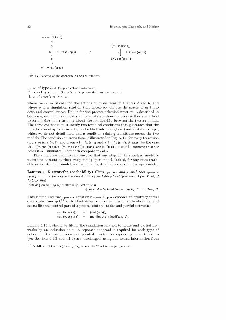
32 Bourke, van Glabbeek, and Höfner
σ i = fst (sr s)∧s (σ, snd(sr s))
=⇒
s’ (σ’, snd(sr s’))∧
σ’ i = fst (sr s’)
a ∈ trans (np i) a ∈ trans (onp i)
Fig. 17 Schema of the openproc np onp sr relation.
1. np of type ip ⇒ (’s, proc-action) automaton ,2. onp of type ip ⇒ ((ip ⇒ ’k) × ’t, proc-action) automaton , and3. sr of type ’s ⇒ ’k × ’t ,
where proc-action stands for the actions on transitions in Figures 2 and 6, andwhere sr is a simulation relation that effectively divides the states of np i intodata and control states. Unlike for the process selection function ps described inSection 4, we cannot simply discard control state elements because they are criticalto formalizing and reasoning about the relationship between the two automata.The three constants must satisfy two technical conditions that guarantee that theinitial states of np i are correctly ‘embedded’ into the (global) initial states of onp i,which we do not detail here, and a condition relating transitions across the twomodels. The condition on transitions is illustrated in Figure 17: for every transition(s, a, s’)∈ trans (np i), and given σ i = fst (sr s) and σ’ i = fst (sr s’), it must be the casethat ((σ, snd (sr s)), a, (σ’, snd (sr s’)))∈ trans (onp i). In other words, openproc np onp srholds if onp simulates np for each component i of σ.
The simulation requirement ensures that any step of the standard model istaken into account by the corresponding open model. Indeed, for any state reach-able in the standard model, a corresponding state is reachable in the open model.
Lemma 4.15 (transfer reachability) Given np, onp, and sr such that openprocnp onp sr, then for any wf-net-tree Ψ and s∈ reachable (closed (pnet np Ψ)) (λ-. True), itfollows that(default (someinit np sr) (netlift sr s), netliftc sr s)
∈ oreachable (oclosed (opnet onp Ψ)) (λ- - -. True) U.
This lemma uses two openproc constants: someinit np sr i chooses an arbitrary initialdata state from np i,15 with which default completes missing state elements, andnetliftc lifts the control part of a process state to nodes and partial networks:
netliftc sr (s iR) = (snd (sr s)) i
R
netliftc sr (s q t) = (netliftc sr s) q (netliftc sr t) .
Lemma 4.15 is shown by lifting the simulation relation to nodes and partial net-works by an induction on Ψ . A separate subproof is required for each type ofaction and the assumptions incorporated into the corresponding open SOS rules(see Sections 4.1.3 and 4.1.4) are ‘discharged’ using contextual information from
15 SOME x. x∈ (fst ◦ sr) ‘ init (np i), where the ‘‘’ is the image operator.

Mechanizing a Process Algebra for Network Protocols 33
the transition in the standard model. The result is that every transition in thestandard model (closed (pnet np Ψ)) is simulated by a transition in the open model(oclosed (opnet onp Ψ)). An implication from an open invariant on an open model toan invariant on the corresponding standard model follows directly.
Corollary 4.16 (transfer) Given np, onp, and sr such that openproc np onp sr, andprovided wf-net-tree Ψ , then from oclosed (opnet onp Ψ) |= (λ- - -. True, U →) (λ(σ,-). P σ),it follows that closed (pnet np Ψ) ||= netglobal np sr P.
In terms of our running example, we first show openproc ptoy optoy id. We thenapply a generic sublocale relation for parallel composition with qmsg to obtainopenproc (λi. ptoy i 〈〈 qmsg) (λi. optoy i 〈〈i qmsg) (λ((ξ, p), q). (ξ, (p, q))), to which we canapply Corollary 4.16 to obtain an appropriate transfer lemma. Compared to thenetglobal constant in Invariant (5), the one in Corollary 4.16 is defined genericallywithin the openproc locale and is therefore parameterized by np and sr. The formeris obtained from the latter by a simple instantiation.
Summary. The technicalities of the lemmas in this and the preceding section areessential for the underlying proofs to succeed. The key idea is that through an openversion of AWN where automaton states are segregated into data and controlcomponents, one can reason locally about global properties, but still, using thetransfer and lifting results, obtain a result over the original model (c.f. Figure 16).
5 Concluding remarks
We present a mechanization of AWN, a modelling language for MANET andWMNprotocols, including a streamlined adaptation of standard theory for showing in-variants of individual reactive processes, and a novel and compositional frameworkfor lifting such results to network models. The framework allows the statement andproof of inter-node properties. We think that many elements of our approach wouldapply to similarly structured models in other formalisms.
It is reasonable to ask whether the basic model presented in Section 2 could notsimply be abandoned in favour of the open model of Section 4.1. We believe, how-ever, that the basic model is the most natural way of describing what AWN means,proving semantic properties of the language, showing ‘node-only’ invariants, and,potentially, for showing refinement relations. Having such a reference model allowsus to freely incorporate assumptions into the open SOS rules, knowing that theirsoundness will later be justified.
The AODV case study. The framework we present in this paper was successfullyapplied in the mechanization of a proof of loop freedom [11, §7] of the AODVprotocol [31], a widely-used routing protocol designed for MANETs, and one ofthe four protocols currently standardized by the IETF MANET working group.The model has about 100 control locations across 6 different processes, and usesabout 40 functions to manipulate the data state. The main property (loop freedom)roughly states that ‘a data packet is never sent round in circles without beingdelivered’. To establish this property, we proved around 400 lemmas. Due to thecomplexity of the protocol logic and the length of the proof, we present the detailselsewhere [5]. The case study shows that the presented framework can be appliedto verification tasks of industrial relevance.

34 Bourke, van Glabbeek, and Höfner
Verifying implementations.We argue in the introduction that AWN is well-adaptedfor modelling MANET and WMN protocols due to its support for their data struc-tures and specialized communication primitives, and also because of its operationalstyle. In the rest of the paper, we present techniques for the machine-assisted andcompositional verification of safety properties of networks of cooperating nodes;and we claim that the AODV case study is testament to the effectiveness of thisapproach. An important question remains: are AWN models suitable specificationsfor protocol implementations? For instance, is it feasible to prove that a programwritten in C or a similar programming language correctly implements a sequentialAWN process? Would it be better to try to refine or transform an AWN processinto an executable form? Or simply to analyse network traces against an instan-tiation of the model [2]? In any case, all of these challenges require precise, andideally mechanized, protocol models, and proofs that they satisfy given properties.
Acknowledgements We thank G. Klein and M. Pouzet for their support and complaisance,M. Daum for his participation in early discussions, and T. Sewell for sharing his talent withIsabelle. The tools Isabelle/jEdit [37], Sledgehammer [3], parallel processing [38], and theTPTP project [35] were invaluable.
References
1. Bengtson, J., Parrow, J.: Psi-calculi in Isabelle. In: S. Berghofer, T. Nipkow, C. Urban,M. Wenzel (eds.) Theorem Proving in Higher Order Logics (TPHOLs 2009), LNCS, vol.5674, pp. 99–114. Springer (2009)
2. Bishop, S., Fairbairn, M., Norrish, M., Sewell, P., Smith, M., Wansbrough, K.: Engineeringwith logic: HOL specification and symbolic-evaluation testing for TCP implementations.In: Principles of Programming Languages (POPL’06), pp. 55–66. ACM (2006)
3. Blanchette, J.C., Böhme, S., Paulson, L.C.: Extending Sledgehammer with SMT solvers.In: N. Bjørner, V. Sofronie-Stokkermans (eds.) Conference on Automated Deduction(CADE-23), LNCS, vol. 6803, pp. 116–130. Springer (2011)
4. Bourke, T.: Mechanization of the Algebra for Wireless Networks (AWN). Archive of FormalProofs (2014). http://afp.sf.net/entries/AWN.shtml
5. Bourke, T., van Glabbeek, R.J., Höfner, P.: A mechanized proof of loop freedom of the(untimed) AODV routing protocol. In: F. Cassez, J.F. Raskin (eds.) Automated Tech-nology for Verification and Analysis (ATVA’14), LNCS, vol. 8837, pp. 47–63. Springer(2014)
6. Bourke, T., van Glabbeek, R.J., Höfner, P.: Showing invariance compositionally for aprocess algebra for network protocols. In: G. Klein, R. Gamboa (eds.) Interactive TheoremProving (ITP’14), LNCS, vol. 8558, pp. 144–159. Springer (2014)
7. Bourke, T., Höfner, P.: Loop freedom of the (untimed) aodv routing protocol. Archive ofFormal Proofs (2014). http://afp.sf.net/entries/AODV.shtml
8. Chandy, K.M., Misra, J.: Parallel Program Design: A Foundation. Addison Wesley (1988)9. Chaudhuri, K., Doligez, D., Lamport, L., Merz, S.: Verifying safety properties with the
TLA+ proof system. In: J. Giesl, R. Hähnle (eds.) Int. Joint Conference on AutomatedReasoning (IJCAR’10), LNCS, vol. 6173, pp. 142–148. Springer (2010)
10. Fehnker, A., van Glabbeek, R.J., Höfner, P., McIver, A.K., Portmann, M., Tan, W.L.: Aprocess algebra for wireless mesh networks. In: H. Seidl (ed.) European Symposium onProgramming (ESOP ’12), LNCS, vol. 7211, pp. 295–315. Springer (2012)
11. Fehnker, A., van Glabbeek, R.J., Höfner, P., McIver, A.K., Portmann, M., Tan, W.L.:A process algebra for wireless mesh networks used for modelling, verifying and analysingAODV. Technical Report 5513, NICTA (2013). URL http://arxiv.org/abs/1312.7645
12. Feliachi, A., Gaudel, M.C., Wolff, B.: Isabelle/Circus: A process specification and verifica-tion environment. In: R. Joshi, P. Müller, A. Podelski (eds.) Verified Software: Theories,Tools, and Experiments (VSTTE’12), LNCS, vol. 7152, pp. 243–260. Springer (2012)
13. Floyd, R.W.: Assigning meanings to programs. Proceedings of the Symposia in AppliedMathematics 19, 19–32 (1967)
Mechanizing a Process Algebra for Network Protocols 35
14. Fokkink, W., Groote, J.F., Reniers, M.: Process algebra needs proof methodology. In:EATCS Bulletin 82, pp. 109–125 (2004)
15. Ghassemi, F., Fokkink, W., Movaghar, A.: Restricted broadcast process theory. In:A. Cerone, S. Gruner (eds.) Software Engineering and Formal Methods (SEFM ’08), pp.345–354. IEEE Computer Society (2008)
16. Godskesen, J.C.: A calculus for mobile ad hoc networks. In: A.L. Murphy, J. Vitek (eds.)Coordination Models and Languages (COORDINATION ’07), LNCS, vol. 4467, pp. 132–150. Springer (2007)
17. Göthel, T., Glesner, S.: An approach for machine-assisted verification of Timed CSP spec-ifications. Innovations in Systems and Software Engineering 6(3), 181–193 (2010)
18. Heyd, B., Crégut, P.: A modular coding of UNITY in COQ. In: G. Goos, J. Hartmanis,J. Leeuwen, J. Wright, J. Grundy, J. Harrison (eds.) Theorem Proving in Higher OrderLogics (TPHOLs 1996), LNCS, vol. 1125, pp. 251–266. Springer (1996)
19. Hirschkoff, D.: A full formalisation of π-calculus theory in the Calculus of Constructions.In: K. Schneider, J. Brandt (eds.) Theorem Proving in Higher Order Logics (TPHOLs2007), LNCS, vol. 4732, pp. 153–169. Springer (2007)
20. Kammüller, F., Wenzel, M., Paulson, L.C.: Locales: A sectioning concept for Isabelle. In:Y. Bertot, G. Dowek, A. Hirschowitz, C. Paulin, L. Théry (eds.) Theorem Proving inHigher Order Logics (TPHOLs 1999), LNCS, vol. 1690, pp. 149–165. Springer (1999)
21. Lamport, L.: Specifying Systems: The TLA+ Language and Tools for Hardware and Soft-ware Engineers. Addison Wesley (2002)
22. Lynch, N.A., Tuttle, M.R.: An introduction to input/output automata. CWI Quarterly2(3), 219–246 (1989). URL http://theory.lcs.mit.edu/tds/papers/Lynch/CWI89.html
23. Manna, Z., Pnueli, A.: Temporal Verification of Reactive Systems: Safety. Springer (1995)24. Merro, M.: An observational theory for mobile ad hoc networks (full version). Information
and Computation 207(2), 194–208 (2009)25. Mezzetti, N., Sangiorgi, D.: Towards a calculus for wireless systems. Electronic Notes in
Theoretical Computer Science (ENTCS) 158, 331–353 (2006)26. Milner, R.: Operational and algebraic semantics of concurrent processes. In: J. van
Leeuwen (ed.) Handbook of Theoretical Computer Science, chap. 19, pp. 1201–1242. El-sevier Science Publishers B.V. (North-Holland) (1990). Alternatively see Communicationand Concurrency, Prentice-Hall, Englewood Cliffs, 1989, of which an earlier version ap-peared as A Calculus of Communicating Systems, LNCS 92, Springer, 1980
27. Müller, O.: A verification environment for I/O Automata based on formalized meta-theory.Ph.D. thesis, TU München (1998)
28. Nanz, S., Hankin, C.: A framework for security analysis of mobile wireless networks. The-oretical Computer Science 367, 203–227 (2006)
29. Nipkow, T., Paulson, L.C., Wenzel, M.: Isabelle/HOL: A Proof Assistant for Higher-OrderLogic, LNCS, vol. 2283. Springer (2002)
30. Paulson, L.C.: The inductive approach to verifying cryptographic protocols. Journal ofComputer Security 6(1–2), 85–128 (1998)
31. Perkins, C.E., Belding-Royer, E.M., Das, S.R.: Ad hoc on-demand distance vector (AODV)routing. RFC 3561 (Experimental), Network Working Group (2003)
32. Plotkin, G.: A structural approach to operational semantics. The Journal of Logic andAlgebraic Programming 60–61, 17–139 (2004). Originally appeared in 1981
33. Singh, A., Ramakrishnan, C.R., Smolka, S.A.: A process calculus for mobile ad hoc net-works. Science of Computer Programming 75, 440–469 (2010)
34. de Roever, W.P., de Boer, F., Hannemann, U., Hooman, J., Lakhnech, Y., Poel, M.,Zwiers, J.: Concurrency Verification: Introduction to Compositional and NoncompositionalMethods. Cambridge Tracts in Theoretical Computer Science 54. CUP (2001)
35. Sutcliffe, G.: The TPTP problem library and associated infrastructure: The FOF and CNFparts, v3.5.0. Journal of Automated Reasoning 43(4), 337–362 (2009)
36. Tej, H., Wolff, B.: A corrected failure divergence model for CSP in Isabelle/HOL. In: J.S.Fitzgerald, C.B. Jones, P. Lucas (eds.) Industrial Applications and Strengthened Founda-tions of Formal Methods (FME’97), LNCS, vol. 1313, pp. 318–337. Springer (1997)
37. Wenzel, M.: Isabelle/jEdit—a prover IDE within the PIDE framework. In: J. Jeuring,J.A. Campbell, J. Carette, G. Dos Reis, P. Sojka, M. Wenzel, V. Sorge (eds.) IntelligentComputer Mathematics, LNCS, vol. 7362, pp. 468–471. Springer (2012)
38. Wenzel, M.: Shared-memory multiprocessing for interactive theorem proving. In: S. Blazy,C. Paulin-Mohring, D. Pichardie (eds.) Interactive Theorem Proving (ITP’13), LNCS, vol.7998, pp. 418–434. Springer (2013)
39. Zhou, M., Yang, H., Zhang, X., Wang, J.: The proof of AODV loop freedom. In: Int. Conf.on Wireless Communications and Signal Processing (WCSP’09). IEEE (2009)


![Mechanizing a Process Algebra for Network Protocols · 2 Bourke,vanGlabbeek,andHöfner and Wireless Mesh Networks (WMNs) [10,11], but that can be used for reason-ing about routing](https://img.pdfslide.net/doc/110x75/5ed0cab16d761e663b7d2412/mechanizing-a-process-algebra-for-network-protocols-2-bourkevanglabbeekandhfner.jpg)