Mediated Persuasion

Andrew Kosenko∗

Department of Economics, University of Pittsburgh

This draft: October 31, 2018First draft: October 2017

Abstract

We study a game of strategic information design between a sender, who choosesstate-dependent information structures, a mediator who can then garble the signalsgenerated from these structures and a receiver who takes an action after observingthe signal generated by the first two players. We characterize sufficient conditions forinformation revelation, compare outcomes with and without a mediator and providecomparative statics with regard to the preferences of the sender and the mediator. Wealso provide novel conceptual and computational insights about the set of feasibleposterior beliefs that the sender can induce, and use these results to obtain insightsabout equilibrium outcomes. The sender never benefits from mediation, while the re-ceiver might. The receiver benefits when the mediator’s preferences are not perfectlyaligned with hers; rather the mediator should prefer more information revelation thanthe sender, but less than perfect revelation.

JEL Classification: D82, D83, C72.Keywords: persuasion, strategic communication, information transmission, interme-

diation, noisy communication, Blackwell informativeness, information garbling, strategicinformation provision.

∗ak2912@columbia.edu; I am deeply grateful to Navin Kartik, for his invaluable help and advice. I wouldalso like to thank Yeon-Koo Che and Joseph Stiglitz for guidance and comments from which I have benefitedimmensely, as well as James Best, Ambuj Dewan, Laura Doval, Nate Neligh, Anh Nguyen, Pietro Ortoleva,Daniel Rappoport, Luca Rigotti, Teck Yong Tan, Roee Teper, Richard van Weelden, and the participants ofthe Columbia Microeconomic Theory Colloquium and the Pitt Micro Theory Brown Bag for discussions andinput. The usual disclaimer applies.

1

1 Introduction and Literature Setting

How does the presence of a mediator affect the informational interaction between twoparties? In this paper we study a game of persuasion between one side (a sender) thatis trying to persuade another side (a receiver) to take a certain action; we add to thisstandard environment a mediator who is able to alter the recommendation of the senderin some way, before the receiver takes her action.

The paper has two main contributions. One is technical and concerns computing theset of receiver posterior beliefs that can be induced; we introduce a novel way of solvingthis problem and one that can be used in other settings. In addition, there is a strongparallel between our results, their representation and implications, and the literature onordering information structures.1 The second contribution is more ”economic” in nature,and concerns equilibria of the mediated persuasion game. We consider several econom-ically important classes of utilities (namely, linear, concave, convex and step functions)and provide results about information revelation and welfare in equilibrium for thoseclasses of utilities. Notably, while most papers in this literature focus on the sender’smost preferred equilibria, taking the view that the sender can ”steer” the receiver into theappropriate equilibrium, we also seriously consider the welfare of the receiver across dif-ferent equilibria, taking the view that in most applications, it is the receiver’s welfare thatone cares about ultimately.

The subject of persuasion, broadly construed, is currently being actively investigatedin information economics; much excellent research has been produced in the last few yearson this, and the topic is continuing to prove a fertile ground for models and applications.More particularly, the topic of information design - the study of how information endoge-nously affects incentives and vice versa - is swiftly becoming a major avenue of research.We add an institutional aspect to this research program, and investigate the effects of dif-ferent informational-organizational topologies on information revelation and welfare.

In the model studied here, the sender and the receiver are restricted to communicateindirectly, via an intermediator (perhaps more than one), due to technical or institutionalconstraints. For example, when a financial firm issues certain kinds of financial products,some large (institutional) investors are prohibited from purchasing them, unless they havebeen rated by a third party, and have achieved a certain rating. Similarly, in many orga-nizations (including many firms, the military, and the intelligence community) the flowof information is directed, with the direction exogenously predetermined, with variousagents having the ability to alter (or perhaps not pass on) the information passed up tothem. This is precisely the kind of setting we are concerned with here.

The problem as we have formulated it is quite difficult in general. Here, one strategicplayer (the sender) can both create and destroy information, and the other strategic player(the mediator) can only destroy information that the first player provided, but cannotcreate any new information, and in addition, both2 of these players only have probabilisticcontrol over evidence realization.

1We pursue this line of inquiry in a contemporaneous related paper.2There is of course the third player - the receiver - but she is effectively facing a decision problem. The key

interplay is between the sender and the mediator.

2

One of the major difficulties is that when the mediator changes her action, not onlydoes the sender’s best response generically change (this is, of course, at the heart of allgame-theoretic models), but the effective choice set of the sender changes as well. Weovercome this problem and show how to compute explicitly the feasible sets for the me-diator the and the sender as functions of the sender’s and the mediator’s actions.

As a consequence of the modeling assumptions, it will turn out that given the choiceof the sender, the mediator can deviate to anything less informative in the sense of DavidBlackwell, while given the choice of the mediator the sender can deviate to some thingsthat are less Blackwell informative (than the implied final experiment), but not everything.What these ”some” things are is precisely what we characterize in the first part of thepaper.

This is also what makes our work different. The major thrust of the literature on multi-sender Bayesian persuasion has focused on players only being able to add (in a certainsense) information.3 On the other hand, the contemporaneous work on persuasion withnoise (where some information is exogenously destroyed) has studied nonstrategic set-tings. We consider an environment where some players can add information, some cansubtract information, and in addition, we study a game, not a decision problem. Fur-thermore, we compare outcomes of the game along two dimensions; first we vary thepreferences of the sender and he mediator. The most prominent result is that (perhapsunsurprisingly) preference divergence ”quickly” leads to the only equilibrium being unin-formative. The final object of this exercise is to compare outcomes (for fixed preferences),in terms of information revelation and welfare, between standard Bayesian persuasion,and Bayesian persuasion with an informational mediator. We show that although the me-diator can only destroy information (in an appropriate sense), this can still result in a strictincrease in the amount of information revealed in a very strong sense - Blackwell domi-nance. In simple, common, and non-pathological environments we show that mediationcannot lead to an increase in information revelation. Moreover, in these environments me-diation of the sort we discuss has unambiguous detrimental effects on the welfare of thekey players. This is not, however, true in general, as we show by illuminating examples.

A ”complete” solution to this problem is, of course, the following: explicitly exhibitthe actions chosen, and the equilibrium outcomes (belief distributions) as functions ofarbitrary utilities of the players. We will not solve the problem at this level of generality.Rather, we will solve some economically important special cases, and comment informallyupon features of the general outcomes in the conclusion.

Our work provides a foundation for analyzing when informational mediation of thesort we discuss is actually beneficial to the receiver.4 In other words, given some prefer-ences for the players, when would the receiver (with those preferences) prefer to play the

3For example, in the Gentzkow and Kamenica work on this problem they identify a condition - Blackwell-connectedness - which ensures that full revelation is always an equilibrium outcome in their multisendergame. The condition says that given the information provided by the others, any individual player can al-ways deviate to something more informative. Li and Normal similarly assume that each sequential player hasaccess to signals that are arbitrarily correlated, so that a player can improve upon the information providedby others realization by realization. In both cases any one player can unilaterally increase the amount ofinformation provided.

4Obviously, it is never strictly beneficial to the sender.

3

game with a mediator to playing the same game with the same preferences but withouta mediator? The answer, perhaps unsurprisingly, is sometimes yes, sometimes no, de-pending on the preferences. The second main contribution of the paper is in providingexamples and analyzing some important base cases, such as when the relevant utilitiesare linear, strictly concave and convex, or are step functions.

This work is at the intersection of two literatures - strategic information design andnoisy persuasion/communication. Our work relies on some results, and is in the spiritof, the celebrated ”Bayesian persuasion” approach of Kamenica and Gentzkow (2011)(referred to simply as ”KG” for brevity hereafter) who consider a simpler version of thisproblem, and discuss an application of a certain concavification result first considered inchapter 1 of Aumann and Maschler (1995). Sah and Stiglitz (1986) introduced the analysisof economic systems organized in parallel and in series; hierarchies and polyarchies ofpersuasion via provision of information have already been explored in previous work(Gentzkow and Kamenica (2017a) (referred to as ”GK” henceforth, not to be confusedwith ”KG”),

There are a number of papers that are closely related to the present model. One is Am-brus, Azevedo and Kamada (2013) which considers a cheap talk model where the senderand receiver also communicate via chains of intermediators. Our work is similar in thattalk is ”cheap” here as well, meaning that the specific choices of the sender and the me-diators do not enter their utility functions directly and only do so through the action ofthe receiver; in addition, we, too, have an analogous communication sequence. The dif-ference is that the sender is not perfectly informed about the state, the message she sendsdepends on the state, and is in general, stochastic. Li and Norman (2018)’s paper on se-quential persuasion serves as another stepping stone - they have a very similar model ofpersuasion, except that the senders move sequentially, observing the history of actionsof the senders who moved before them (unlike in our model), and can provide arbitrar-ily correlated experiments. The other relevant work is Gentzkow and Kamenica (2017)’swork on competition in persuasion where the senders move simultaneously (like in ourmodel), but all senders are trying to provide information about the state of the world,whereas we study an environment where the mediator is trying to provide informationabout the realization of the sender’s experiment. Lipnowski, Ravid and Shishkin (2018)also study a related environment where a ”weak institution” in their parlance plays therole of a kind of informational mediator, although the setup is considerably different andthere is no role for the interplay of preferences which we focus on here. The subject ofintroducing a mediator to potentially improve outcomes has also been studied in contracttheory (see, inter alia, Pollrich (2017) and Rahman and Obara (2010)).

Perez-Richet and Skreta (2018) present a complementary model that differs in one keyrespect - the mediator (using our nomenclature) moves first and her choice is observed bythe sender before the sender acts. Our focus is on analyzing outcomes of a particular gameas one changes preferences for the mediator (and fixing the signal realization spaces in ad-vance), while they focus on equilibria of a game where the preferences of the mediator arealways fully aligned with those of the receiver. More specifically, they construct a ”test”where the sender/persuader employs a continuum of signal realizations to pass or fail

4

different types of sender. Plainly, the difference between our work and theirs is that wefix the signal realization space and vary the preferences of the players, while they fix thepreferences and derive the optimal signal realization space (and signal realization prob-abilities). Notably, the contrast with Perez-Richet and Skreta (2018) immediately showsthat it is strictly with loss of generality to restrict the space of signal realizations, as we doin the paper. This assumption, however, greatly simplifies our problem.5

Strulovici (2017) in his ”Mediated Truth” paper explores a somewhat related environ-ment where a ”mediator” - an expert of some sort or a law enforcement officer - has accessto information that is ”costly to acquire, cheap to manipulate and produced sequentially”.He shows that when information is reproducible and not asymptotically scarce (for exam-ple, one can perform many scientific experiments) then societies will learn the truth, whilewhen information is limited (such as evidence from a crime) the answer is negative. Inour work we consider a one-shot game, but his insight provides an interesting contrast.For example, a repeated version of the game considered here would satisfy the conditionfor evidence to not be asymptotically scare, however, it is not clear that this is enough toovercome the incentive problem when the mediator can only garble the signals; certainlythere will be no learning is the unique equilibrium in our model is uninformative, as canbe the case.

Le Treust and Tomala (2018) study a very similar, but simpler setting. They considerpersuasion with an additional constraint - exogenous noise - and show that while thesender generically suffers a loss as a result of the noise, information-theoretic tools showthat the sender can do as well as possible, provided she plays the game enough times (i.e.enough independent copies of the same basic problem are available). Their model can beviewed as a (repeated) special case of the model studied in our paper, with a nonstrategicmediator.

Tsakas and Tsakas (2018) also study the problem of Bayesian persuasion subject toexogenous noise. They show that while it is in principle possible for the sender to benefitfrom noise, they obtain analogous results to ours (that the senderdo is always worse offwith more noise) when comparing similar noise structures. The reason for why in ourmodel the sender is always worse off, and in their model the sender can be better off is thatthey consider additional noise structures (which they refer to as ”partitional” channels),and the sender may be better off when faced with noise structures that are both canonicaland partitional. Thus, our work agrees with theirs along the dimension along which theenvironments are comparable, but we also consider strategic interaction.

Ichihashi (2017) studies a model in which the sender’s information may be limited; hefocuses on the cases where doing so might benefit the receiver. In our model a similar roleis played by the mediator who modifies the information produced by the sender, and canonly modify it by garbling (i.e. only decreasing the amount of information). Thus, whileIchihashi (2017) limits the sender’s information, we limit what the sender can do with thatinformation.

5Indeed, if one were to consider a problem of which both this paper and Perez-Richet and Skreta (2018) arespecial cases, one would have a strategic problem with an unrestricted domain of utilities with complicatedinfinite-dimensional action spaces.

5

We study a game where the players move simultaneously (this is just a modeling trickof course - they do not have to actually act at the same time - the reason for this is becausetypically one party is not aware of the ratings mechanism or the choice of the financial in-struments of the other party when committing to an action; it could also be simply becausea player is unable to detect deviations in time to adjust their own strategy); the key pointis that the mediator does not see the choice of the sender before making her own choice asin some other models. In other words, we assume ”double commitment” - commitment toan information structure for the sender and the mediator, along the lines discussed in KG.This feature generates an interesting possibility of having a kind of prisoner’s dilemmanot in actions, but in information.6 The flow of information is path-dependent (as in Liand Norman (2018)), yet not quite sequential while action choices for the sender and themediator are simultaneous.

Our focus will be on the amount of information revealed in various organizationalsetups and the effect of competition and preference (mis)alignment on information rev-elation and outcomes. Although the basic model is quite general, we have in mind oneparticular application - the design of a ratings agency. A rating assigned to a financialproduct can be thought of as an expression of likelihood of default or expected economicloss. A firm (in the parlance of the present setting, the sender) chooses strategically whatevidence to submit to a rater (here, the mediator). The mediator, perhaps driven by con-cerns that may not be identical to those of the firm, then rates the evidence submittedby the firm, and issues a recommendation to the client or the public. We analyze theeffect on informativeness and welfare of the mediator’s presence in this informational-organizational topology.

There are several features of this real-world example that deserve mention. First notethat the issuing firm itself cannot rate its own financial products; it does, however, designits products (or at least gets to choose the products that it submits for review at a particularinstance). The ratings agency cannot choose the products - it is constrained to rate thepackage it has been submitted, but it can choose its ratings process and criteria. It alsoexhibits the criteria according to which it issued its conclusions. Finally, the purchaser ofthe financial products (the receiver) is often required to only buy products that have beenrated by a reputable firm - in other words, there is an institutional constraint at work.

To take a specific example consider structured finance products that consisted of var-ious repackagings of individual loans (mortgages were by far the most important com-ponent) into so-called structured investment vehicles, or SIVs. The financial firms issuedproducts that consisted of bundles of individual mortgages, along with rules for obtain-ing streams of payments from those mortgages. These streams were correlated with eachother (since two nearby houses were in the same area, the local economic conditions thataffected the ability of one lender to repay, also affected the ability of the other lender torepay), as well as with the overall economy. The firms chose the specific mortgages thatwent into each SIV strategically. The ratings agencies then rated these SIVs; however, onekey element in their ratings (and one that was later shown to be partially responsible forthe revealed inaccuracy of those ratings) is that the ratings agencies did not provide their

6This is also discussed in GK.

6

ratings based on the correlations of the returns with the overall economy. Rather, theirratings consisted (mostly) of evaluations of correlations of individual financial productsin an SIV with each other. The issuer clearly wants to achieve as high a rating as possi-ble7, but if the preferences of the mediator are to ”collude” with the seller, this essentiallymeans that there may be very little information revelation in equilibrium.

In this example the state of the world is a complete, fully specified joint distribution ofreturns; an experiment is a mapping from states of the world into a set that specifies onlypartial information about the correlations (for example, individual correlations).8 Themediator then designs a signal (a rating procedure) that maps information about individ-ual correlations into a scaled rating. The precise ratings methodologies are proprietary,so it makes sense to assume that the sender does not know the strategy of the mediator.This example, although it is meant to be suggestive, is not completely analogous to thesituation we study. We view the model presented in this paper as a normative exercise,descriptive of interesting features of a problem, but not identical to actual ratings process.

In single-issuer bonds, ratings are mute about correlations with other bonds or withthe market. In 2007, less than 1% of corporate issues but 60% of all structured productswere rated AAA. 27 of 30 AAA issues underwritten by Merril Lynch in 2007, were by2008 rated as speculative (”junk”) (See Coval, Jurek and Stafford (2008)). We suggest thata possible explanation for this is that if the mediator is unable to provide new informa-tion, and is only able to ”garble” or rely on the information provided to it by the issuer,then the equilibria in general will not be very informative (and in fact, as the preferencesof the mediator and the sender diverge, the only equilibrium that survives is uninforma-tive). This reasoning suggests a policy proposal - requiring the ratings agencies to performindependent analysis (say, additional ”stress tests”) on the products they are rating, to in-crease the informativeness of the rating; another way of increasing information revelationis to ensure that the preferences of the mediator are what they are prescribed to be by thiswork.

Another (perhaps more closely parallel, but certainly less important) example of thissetting might be the design of a spam filter for an email system.

In what follows we investigate the effect of adding a mediator to a persuasion envi-ronment as well as the welfare implications (for all parties) of varying the alignment ofpreferences of the sender and the mediator. In addition, we consider the effect of addingadditional mediators. Finally, we give a novel characterization of the set of feasible beliefsfor this game and discuss its several interesting features. We do not give a full character-ization of equilibria as a function of preferences (this is a difficult fixed point problem);rather, we give suggestive examples and provide intuition.

7And in fact, there is evidence in structured finance that the firms did design their products so that thesenior tranches would be as large as possible, while still getting the highest possible rating.

8The ”big three” firms all utilize fairly coarse scales for ratings.

7

2 Environment

We study a game with n ≥ 3 players; The first player is called the sender and the lastplayer is called the receiver. The remaining players are the mediators; if there are more thanone of them, we also specify the order in which their probabilistic strategies are executed.

We fix a finite state space, Ω (consisting of nΩ elements) and a finite realization space9

E (consisting of nE elements), where to avoid unnecessary trivialities, the cardinality ofthe set of signals is weakly greater than that of the set of states. An experiment for thesender is a distribution over the set E, for each state of the world: X : Ω → ∆(E); denoteby X the set of available experiments. We assume that X contains both the uninformativeexperiment (one where the probabilities of all experiment realizations are independent ofthe state) and the fully revealing experiment (where each state is revealed with probabilityone). To distinguish between the choices of the sender and those of the mediator, wedefine a signal for the mediator to be a function Σ : E → ∆(S) where S is the space ofsignal realizations containing nS elements; let Σ denote the set of available experiments.Put differently, the mediator is choosing distributions of signal realizations conditionalon realizations of experiments. All available experiments and signals have the same cost,which we normalize to zero. We also refer to either an experiment, or a signal, or theirproduct, generically as an information structure. Since the state space and all realizationspaces are finite, we represent information structures as column-stochastic matrices withthe (i, j)’th entry being the probability of realization i conditional on j. Finally, the receivertakes an action from a finite set A (with nA elements; we assume that nA ≥ nS = nE ≥ nΩ

to avoid trivialities associated with signal and action spaces not being ”rich” enough).The utility of the sender is denoted by uS(ω, a), that of the mediator by uM(ω, a) and thatof the receiver by uR(ω, a). We assume for concreteness that if the receiver is indifferentbetween two or more actions given some belief, he takes the action that is best for thesender.

This setup is capturing one of the key features of our model - the space of realizationsof experiments for one player is the state space for the other player. In other words,both the sender and the mediator are choosing standard Blackwell experiments, but withdifferent state and realization spaces.

For clarity, we summarize the notation used at this point: we use the convention thatcapital Greek letters (X, Σ) refer to the distributions, bold capital Greek letters (X, Σ) re-fer to sets of distributions, capital English letters (E, S) refer to spaces of realizations forinformation structures, and small English letters (e, s) refer to particular realizations.

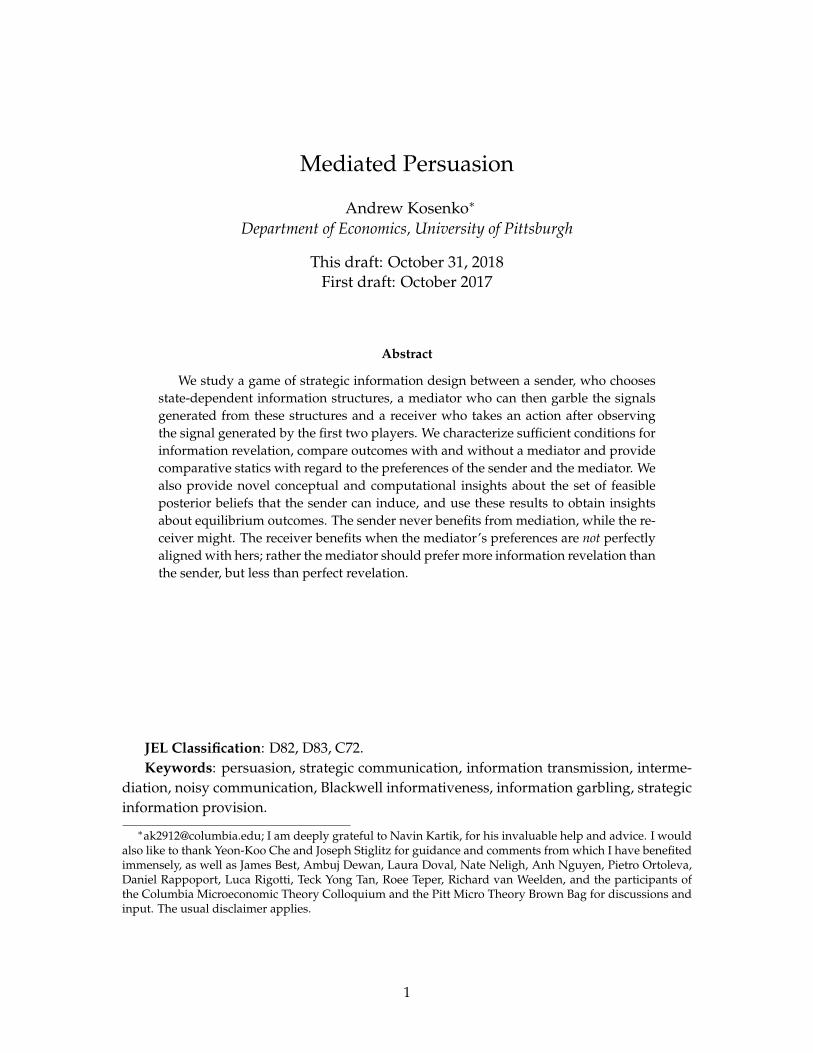
The timing of the game is fairly simple: the sender and the mediator choose their ac-tions simultaneously, while the receiver observes the choices of the experiment, the signal,and the signal realization, but not the experiment realization. The mediator does not ob-serve the choice of the sender when choosing her own action; if he did observe the choice(but not the experiment realization), this would be a special case of the model of sequen-tial persuasion of Li and Norman (2018). If the mediator in addition could observe the

9Typically, the realization space is part of the choice of the sender; here we fix this space (while keeping it”rich enough”) to isolate the effects of mediated persuasion.

8

Nature

State, ω e s a

Sender Mediator Receiver

X

Experiment

Σ

Signal

Figure 1: Illustration of the Model: Flow of Information and Actions.

β0 10

β(X, eL) β(X, eH)0 1

0 1β(ΣX, sL) β(ΣX, sH)

Figure 2: Effect of Garbling on Beliefs in a Dichotomy.

experiment realization (and could therefore condition her own action upon it), this wouldbe similar to the models of persuasion with private information by Hedlund (2017) andKosenko (2018) since then the mediator would have an informational ”type”. Note thatno player observes the realization of the experiment, yet that realization clearly still playsa role in determining outcomes. We focus on pure strategies for all players in the presentwork; a diagram of the main features, nomenclature, timing, and notational conventionsof the model is in figure 1.

The following definition will be extremely useful in what follows:

Definition 1. Let f and g be two probability mass functions on a finite set X = x1, x2, ..., xk ∈Rn. We say that f is a mean-preserving spread of g if there is a (k× k) Markov matrix TK×K =

(t(xi|xJ))ij) such that

i) Tg=f.

ii) For each j = 1, ...k, ∑i T(xi|xj)xj = xj

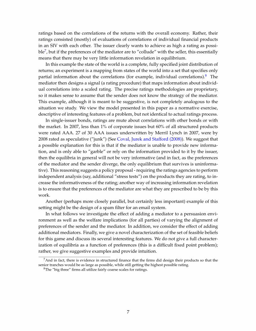
We can also illustrate the effect of a garbling of the experiment by the signal on thebeliefs (as seen in figure 2). In that figure all players start with a common prior, β0. Whenthe sender chooses her experiment X, the two possible beliefs (one for each possible re-alization of the experiment) are a mean-preserving spread of the prior. Following that

9

mediator’s choice of signal, M brings beliefs back in in a mean-preserving contraction. Inother words, in terms of figure 2, we can say that the mediator chooses the length (but notthe location) of the two arrows, and the sender chooses the outer endpoint for each arrow.The inner point of each arrow represents the final beliefs.

Denote by βA(ω|s) the posterior belief of the receiver that the state of the world is ω,computed after observing information structure A, and a signal realization s and denoteby βA(s) the full distribution. We will also find it convenient to refer to distributionsof distributions, which we will denote by τ so that τA(β) is the expected distribution ofposterior beliefs given some generic information structure A:

τA(β) , ∑s∈supp(A)|βA(s)=β

∑ω∈Ω

A(s|ω)β0(ω) (1)

We assume that the set of available experiments is anything (or in any case, ”richenough”). In the present work we focus exclusively on pure strategies for all players. Thisis a major drawback, since as we will see, this environment may have a kind of ”matchingpennies” flavor where both players constantly want to change their action given what theother is doing (and in particular, finding pure strategy equilibria is quite hard). Nonethe-less we make this restriction for simplicity.

Given a receiver posterior belief (we suppress the arguments for notational compact-ness) β, let a∗(β) denote the optimal action of the receiver. Analogously to KG, if twoactions for a sender or a mediator result in the same final belief for the receiver, they areequivalent. We can therefore reduce the number of arguments in the utility functions andwrite uR(β), uM(β), uS(β) (with ui(β) , Eβui(a∗(β), ω), as is customary), and also, withan abuse of notation, uR(τ), uM(τ), uS(τ).

We can begin by observing that an equilibrium exists, and in particular, there is anequilibrium analogous to the ”babbling” equilibria of cheap talk models. Suppose forinstance, that the sender chooses a completely uninformative experiment. Then the me-diator is indifferent between all possible signals, since given the sender’s choice, theycannot affect the action of the receiver; in particular he can choose the uninformative sig-nal as well. Clearly, no player can profitably deviate, given the other’s choices, and thusthis is an equilibrium, which we note in the following

Proposition 1. There exists an uninformative equilibrium.

Along the same line of thinking, we have

Proposition 2. Suppose that either uS or uM (or both) is globally concave over the set of β ∈∆(Ω). Then the unique equilibrium is uninformative.

The proof of this proposition is immediate from inspection of the utilities (if eitherutility is concave, then the player with that utility can always bring beliefs back to theprior, which she would prefer to any other outcome); it is also a sufficient condition forthe only equilibrium to be uninformative.

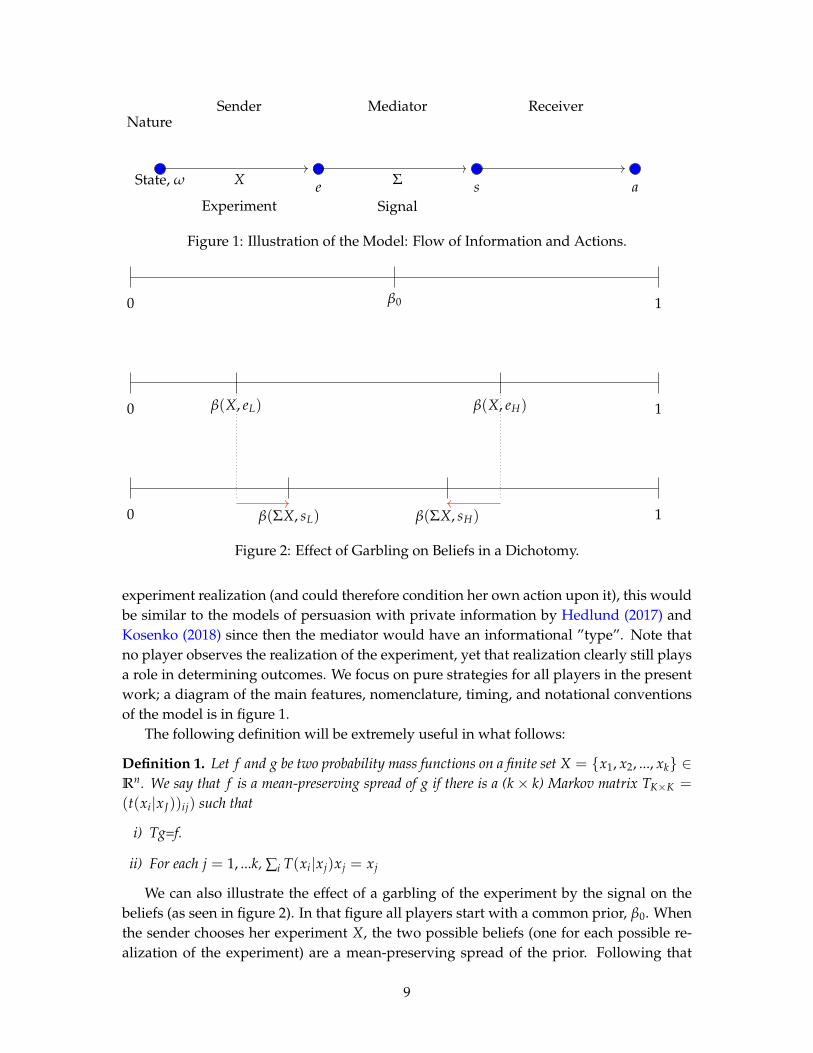
As for nontrivial equilibria, given any X, the mediator’s problem is now similar to theone faced by the sender in KG: choose a Σ such that the distribution of beliefs induced byB is optimal. Formally, the problem for the mediator is:

10

Σ∗ ∈ arg maxΣ∈Σ|ΣX=B

EτuM(β) (2)

τ = p(B) (3)

s.t. ∑s∈supp(Σ)

βR(s)PB(e) = β0 (4)

Similarly, for the sender the problem is

X∗ ∈ arg maxX∈X|ΣX=B

EτuS(β) (5)

τ = p(B) (6)

s.t. ∑s∈supp(Σ)

βR(s)PB(e) = β0 (7)

Let p : MnS,nΩ → ∆(∆(Ω)) whereMnS,nΩ([0, 1]) denotes the set of nS × nΩ column-stochastic matrices be the mapping between an information structure and the space ofposterior beliefs. In other words, p maps a column-stochastic matrix into a distributionover posteriors: p(B) = τ.

We call a pair (X, Σ) that solve the above problems simply an equilibrium and oursolution concept is perfect Bayesian equilibrium. We utilize the power of subgame per-fection to avoid equilibria in which the receiver threatens to take the worst possible actionfor the sender unless he observes the fully revealing experiment, and the worst possibleaction for the mediator unless he observes a fully revealing signal.

One may notice that the matrix equation ΣX = B is precisely the definition for X to bemore Blackwell-informative than B, with Σ being the garbling matrix. We will rely on thisfact (as well as the different and related implications of this fact) throughout what is tofollow. One can make the simple observation that the set of Blackwell-ranked informationstructures forms a chain when viewed as a subset of the set of all information structures.

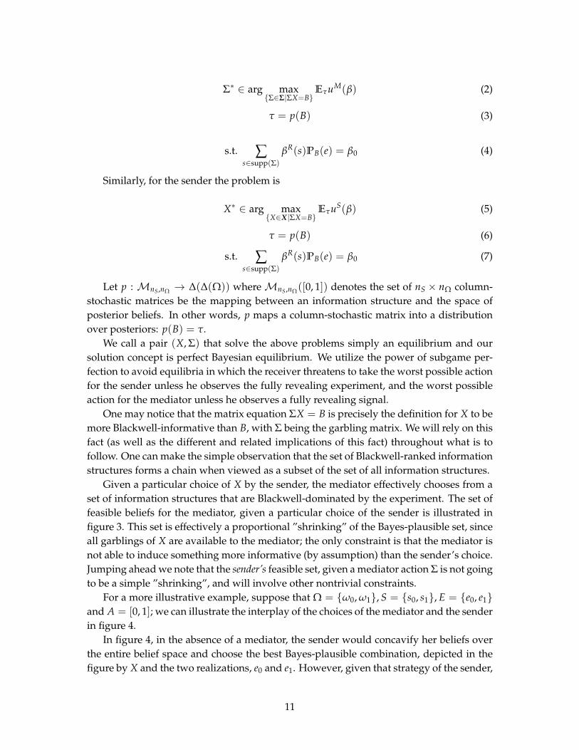
Given a particular choice of X by the sender, the mediator effectively chooses from aset of information structures that are Blackwell-dominated by the experiment. The set offeasible beliefs for the mediator, given a particular choice of the sender is illustrated infigure 3. This set is effectively a proportional ”shrinking” of the Bayes-plausible set, sinceall garblings of X are available to the mediator; the only constraint is that the mediator isnot able to induce something more informative (by assumption) than the sender’s choice.Jumping ahead we note that the sender’s feasible set, given a mediator action Σ is not goingto be a simple ”shrinking”, and will involve other nontrivial constraints.

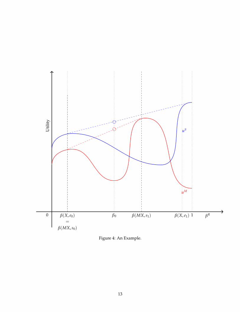
For a more illustrative example, suppose that Ω = ω0, ω1, S = s0, s1, E = e0, e1and A = [0, 1]; we can illustrate the interplay of the choices of the mediator and the senderin figure 4.

In figure 4, in the absence of a mediator, the sender would concavify her beliefs overthe entire belief space and choose the best Bayes-plausible combination, depicted in thefigure by X and the two realizations, e0 and e1. However, given that strategy of the sender,

11

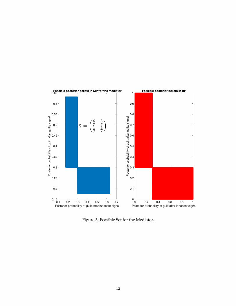
X =

( 67

37

17

47

)

Figure 3: Feasible Set for the Mediator.

12

βR10 β0β(X, e0)

=

β(MX, s0)

β(X, e1)β(MX, s1)

uS

uM

Uti

lity

Figure 4: An Example.

13

the mediator now has an incentive to concavify beliefs over the interval between β(X, e0)

and β(X, e1); as drawn she would prefer to keep the left belief where it was and shiftthe right belief inward; this yield a much higher level of utility. However, note that thesender is now much worse off (and in fact, may be even worse off than she would be hadshe chosen the babbling experiment in the first place). Now the sender has an incentive tochange her action and provide more information by spreading beliefs outward; this kindof interplay is exactly what we focus on.

One can also view the signal choice as a (possibly stochastic) recommendation from themediator; this would be particularly convenient if one could identify the signal realizationspace with the action space. The receiver observes the choices of both the experiment (bythe sender) and the signal (by the mediator). This view would be akin to the literature oninformation design, and thus the sender would be designing an experiment subject to anobedience requirement. This however, is somewhat different from our setting.

For now we focus on the case of a single mediator, as it’s the simplest, builds intuitionand corresponds most closely with the motivating example.

2.1 Building Intuition: A Benchmark With KG Utilities

One useful illustration of the present model is to compare the outcomes of a particularcase of the mediated persuasion model to the leading example of the Bayesian persuasionmodel presented in KG; doing so also provides a good benchmark for the possible out-comes and builds intuition. To that end, suppose that we take the simple model presentedin KG, keep the preferences the same and the add a mediator. Ω = guilty, innocent, E =

S = g, i and A = convict, acquit, let

uS(a) =

1 if aR = convict

0 otherwise(8)

and

uR(a, ω) =

1 if ω = guilty & aR = convict

1 if ω = innocent & aR = acquit

0 otherwise

(9)

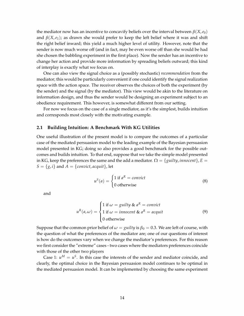
Suppose that the common prior belief of ω = guilty is β0 = 0.3. We are left of course, withthe question of what the preferences of the mediator are; one of our questions of interestis how do the outcomes vary when we change the mediator’s preferences. For this reasonwe first consider the ”extreme” cases - two cases where the mediators preferences coincidewith those of the other two players

Case 1: uM = uS. In this case the interests of the sender and mediator coincide, andclearly, the optimal choice in the Bayesian persuasion model continues to be optimal inthe mediated persuasion model. It can be implemented by choosing the same experiment

14

β0 12

1

1

Figure 5: The KG Setting.

as in the BP model, namely, X =

innocent guilty( )innocent 4

7 0guilty 3

7 1, and Σ =

i g( )i 1 0g 0 1

. The

product ΣX would then clearly yield the desired distribution of signals, and the resultingoptimal distribution of beliefs. For convenience we reproduce the picture from KG infigure 5:

The X and Σ above do not constitute, however, a unique equilibrium. In fact, any pair(Σ, X) with the property that their product results in a Bayes-plausible combination of thebeliefs β = 0 and β = 0.5 is an equilibrium. This simple example shows that the merepresence of a mediator can increase the number of equilibria, but keep the outcome thesame.

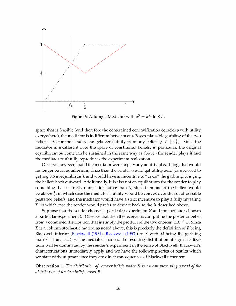
Case 2: uM = uR. We now turn to the question of what happens if the mediator’spreferences are fully aligned with those of the receiver. While intuition suggests that thisarrangement is must be better for the receiver, we show by example that in fact, this doesnot have to be strictly so.10 Writing the mediator’s utility as a function of the receiver’sbelief we obtain

uM(β) =

1− β if β < 1

2

β if β ≥ 12

which we plot on figure 6 in red.The concavification of uM over the entire belief space (which we do not depict) is

simply a straight line at 1. If the sender induces the same two beliefs (β = 0 and β = 0.5)as in the base case, since any garbling of these two beliefs would induce beliefs that areinterior to the set [0, 0.5] and since the mediator’s utility is linear in the subset of belief

10In fact, later we show that more generally, the receiver benefits from persuasion when the mediator’spreferences are not fully aligned with those of the receiver.

15

β0 12

1

1

12

Figure 6: Adding a Mediator with uS = uM to KG.

space that is feasible (and therefore the constrained concavification coincides with utilityeverywhere), the mediator is indifferent between any Bayes-plausible garbling of the twobeliefs. As for the sender, she gets zero utility from any beliefs β ∈ [0, 1

2 ). Since themediator is indifferent over the space of constrained beliefs, in particular, the originalequilibrium outcome can be sustained in the same way as above - the sender plays X andthe mediator truthfully reproduces the experiment realization.

Observe however, that if the mediator were to play any nontrivial garbling, that wouldno longer be an equilibrium, since then the sender would get utility zero (as opposed togetting 0.6 in equilibrium), and would have an incentive to ”undo” the garbling, bringingthe beliefs back outward. Additionally, it is also not an equilibrium for the sender to playsomething that is strictly more informative than X, since then one of the beliefs wouldbe above 1

2 , in which case the mediator’s utility would be convex over the set of possibleposterior beliefs, and the mediator would have a strict incentive to play a fully revealingΣ, in which case the sender would prefer to deviate back to the X described above.

Suppose that the sender chooses a particular experiment X and the mediator choosesa particular experiment Σ. Observe that then the receiver is computing the posterior belieffrom a combined distribution that is simply the product of the two choices: ΣX , B. SinceΣ is a column-stochastic matrix, as noted above, this is precisely the definition of B beingBlackwell-inferior (Blackwell (1951), Blackwell (1953)) to X with M being the garblingmatrix. Thus, whatever the mediator chooses, the resulting distribution of signal realiza-tions will be dominated by the sender’s experiment in the sense of Blackwell. Blackwell’scharacterizations immediately apply and we have the following series of results whichwe state without proof since they are direct consequences of Blackwell’s theorem.

Observation 1. The distribution of receiver beliefs under X is a mean-preserving spread of thedistribution of receiver beliefs under B.

16

It is immediate that if the sender and the mediator have the same preferences, fullrevelation may not be an equilibrium (in that case the set of nontrivial equilibrium out-comes coincides with that in KG). In Gentzkow and Kamenica (2017a) and Gentzkow andKamenica (2017b) full revelation is typically an equilibrium (with at least two senders);the reason is that they identify a condition on the informational environment (”Blackwell-connectedness”) which guarantees that each player can unilaterally deviate to a Blackwell-more informative outcome, regardless of the actions of the other player. Preference diver-gence then forces full revelation. Finally, adding senders does not make the uninformativeequilibrium disappear.

3 Binary Model

For tractability we work with a binary model where there are two states of the worldand two experiment and signal realizations. This is with (perhaps significant) loss ofgenerality, but will serve well to illustrate the basic idea of how to compute a best responsefor the sender given the choice of the mediator.

3.1 Computing the Set of Feasible Posteriors

Setting aside the issues of strategic behavior for now, we first ask a simpler question:given a fixed11 signal (or equivalently, a fixed garbling), or a fixed experiment, what are allthe posterior distributions that can be induced? At this point we can make an importantconnection with the cheap talk and communication literature. Blume, Board and Kawa-mura (2007) discuss a model of cheap talk where the signal sent by the sender is subjectto random error - with a small probability the message observed by the receiver is notthe message sent by the sender, but rather, a message sent from some other distributionthat does not depend on the sender’s type or the message chosen. We make this con-nection to note that choosing an information structure that will be subjected to a fixed,non-strategically-chosen garbling is exactly equivalent to choosing a random signal thatwill be subject to noise. Thus, our model subsumes a model on Bayesian persuasion withnoisy communication, similar to those studied by Le Treust and Tomala (2018) and Tsakasand Tsakas (2018).

In the (different but related) setting of cheap talk, as noted by Ambrus, Azevedo andKamada (2013) as well as Blume, Board and Kawamura (2007) stochastic reports makeincentive compatibility constraints easier to satisfy. This will not quite be the case here,but this will nevertheless be an illuminating exercise.

As mentioned above, for tractability12 we will work in the simplest possible environ-ment of binary signal and state spaces for both the sender and the mediator. In additionto being the simplest nontrivial example of the problem we are trying to solve, workingwith two-by-two square matrices has a very important additional advantage. The rank ofsuch a stochastic13 matrix can be only two things - one or two. If the rank of a two-by-two

11I.e. not strategically chosen by a player as a function of her preferences.12And with loss of generality, which we discuss later.13Which of course, rules out the zero matrix, which has rank zero.

17

stochastic matrix is one, that means that not only the columns (and rows) are linearly de-pendent, but they must, in fact be identical. In that case the garbling is fully uninformative- it can be readily checked that this results in the same posteriors as the canonical com-plete garbling; namely, the posterior (after either signal realization) is equal to the prior.The other possible case is that the matrix has rank two - but that automatically means thatsuch a matrix is invertible. We shall use this fact of existence of an inverse extensively14.

More specifically, let ε be a small positive number, set the space of experiment real-izations to be E = eL, eH and suppose that the sender and receiver play a game exactlyidentical to KG (that is, there is no mediator), except that with probability ε the signalobserved by the receiver (denoted by eo) is not the signal sent (which we denote by es),

but a signal chosen from the following distribution eo =

eH with probability p

eL with probability 1− pThe key thing is that this distribution is independent of both the type and the signal

realized. Thus, we can compute the probabilities of observed signals as functions of theparameters and realized signals as usual:

P(eo = eH |es = eH) = 1− ε + εp (10)

P(eo = eL|es = eH) = ε− εp (11)

P(eo = eL|es = eL) = 1− εp (12)

P(eo = eH |es = eL) = εp (13)

Then this is equivalent to having a garbling

Σ =

(σ1 σ2

1− σ1 1− σ2

)=

(εp− ε + 1 εp

ε− εp 1− εp

)(14)

with realization space S = eoL, eo

H.

If we denote by X =

(x y

1− x 1− y

)the experiment chosen by the sender so that

B = ΣX =

(x(εp− ε + 1)− εp(x− 1) y(εp− ε + 1)− εp(y− 1)(εp− 1)(x− 1) + x(ε− εp) (εp− 1)(y− 1) + y(ε− εp)

)(15)

is the resulting distribution of signal observations given states. Letting Ω = ωH, ωL bethe set of states and setting prior belief of ωL = π the posterior beliefs are

β(sH) = P(ωL|sH) =π [y(εp− ε + 1)− εp(y− 1)]

π [y(εp− ε + 1)− εp(y− 1)] + (1− π) [x(εp− ε + 1)− εp(x− 1)](16)

14We also comment on the interpretation of the rank of a garbling matrix later in the discussion, and inrelated contemporaneous work

18

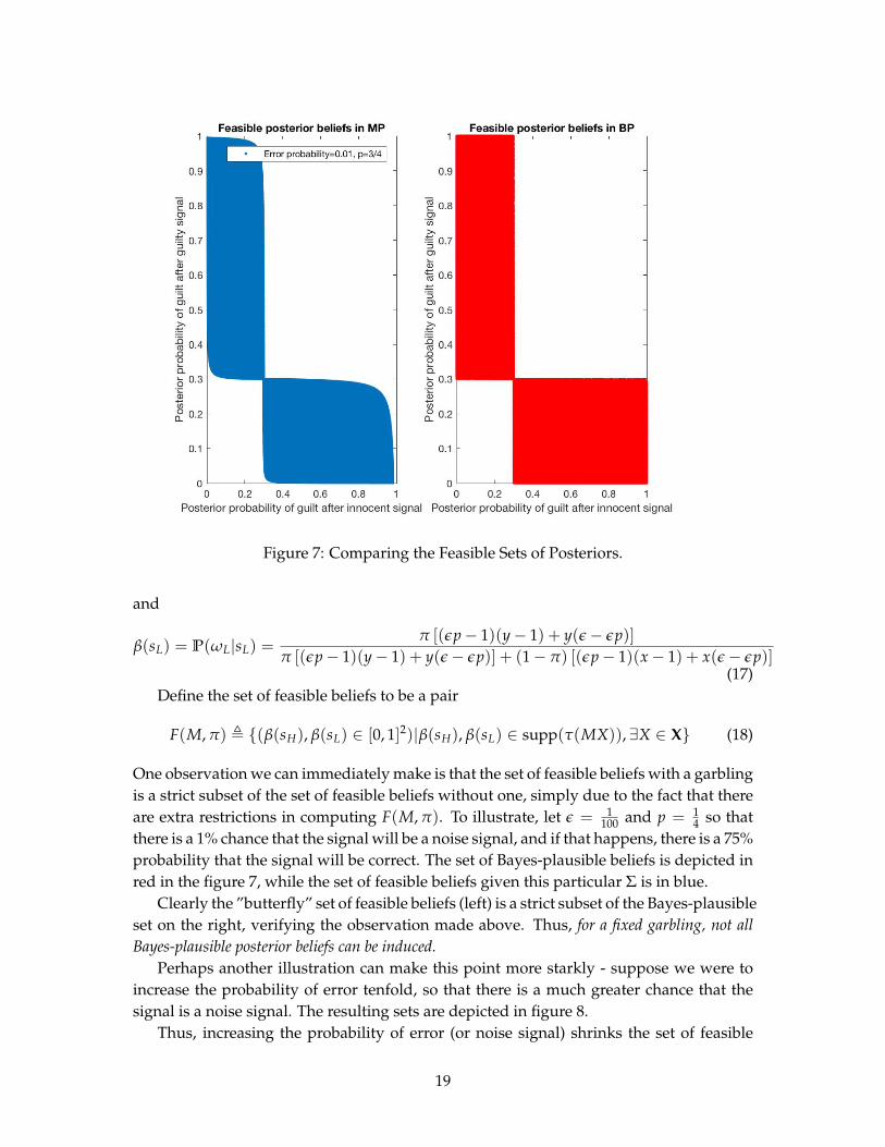
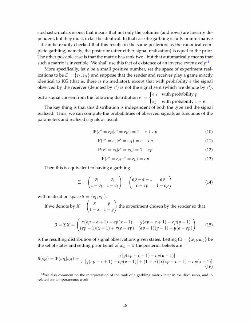
Figure 7: Comparing the Feasible Sets of Posteriors.

and

β(sL) = P(ωL|sL) =π [(εp− 1)(y− 1) + y(ε− εp)]

π [(εp− 1)(y− 1) + y(ε− εp)] + (1− π) [(εp− 1)(x− 1) + x(ε− εp)](17)

Define the set of feasible beliefs to be a pair

F(M, π) , (β(sH), β(sL) ∈ [0, 1]2)|β(sH), β(sL) ∈ supp(τ(MX)), ∃X ∈ X (18)

One observation we can immediately make is that the set of feasible beliefs with a garblingis a strict subset of the set of feasible beliefs without one, simply due to the fact that thereare extra restrictions in computing F(M, π). To illustrate, let ε = 1

100 and p = 14 so that

there is a 1% chance that the signal will be a noise signal, and if that happens, there is a 75%probability that the signal will be correct. The set of Bayes-plausible beliefs is depicted inred in the figure 7, while the set of feasible beliefs given this particular Σ is in blue.

Clearly the ”butterfly” set of feasible beliefs (left) is a strict subset of the Bayes-plausibleset on the right, verifying the observation made above. Thus, for a fixed garbling, not allBayes-plausible posterior beliefs can be induced.

Perhaps another illustration can make this point more starkly - suppose we were toincrease the probability of error tenfold, so that there is a much greater chance that thesignal is a noise signal. The resulting sets are depicted in figure 8.

Thus, increasing the probability of error (or noise signal) shrinks the set of feasible

19

Figure 8: Increasing Noise Shrinks the Set of Feasible Posteriors.

beliefs. This is consistent with intuition - if the signal is pure noise, then there should notbe any update of beliefs (and thus the set would shrink to a single point at the prior), andwith a larger probability of noise one would update ”less”. We make precise the idea thatwith a less informative garbling ”fewer” posteriors are available below.

This discussion leads to the following question: What is the set of feasible posteriorbeliefs given a garbling (without computing whether or each belief is feasible one by oneas was done in computing the figures above, which were generated by simulating ran-dom matrices with the appropriate stochasticity constraints)? One way of answering thisquestion is to trace out the confines of the feasible set. As luck would have it, there is anobservation we can make that simplifies this a great deal. If we fix one posterior belief(say, β1 the posterior after the innocent signal) and then ask what would the elements Xneed to be to either maximize or minimize the other posterior belief, it turns out that ei-

ther x or y (or both) will always be 1 or 0. We fix Σ =

(σ1 σ2

1− σ1 1− σ2

), let π be the prior

belief and consider X =

(x y

1− x 1− y

). Computing outer limits of F(Σ, π) is equivalent

to the following program:

maxx,y

β2 =π[σ1y + σ2(y− 1)]

π[σ1y + σ2(y− 1)] + (1− π)[σ1x− σ2(x− 1)](19)

20

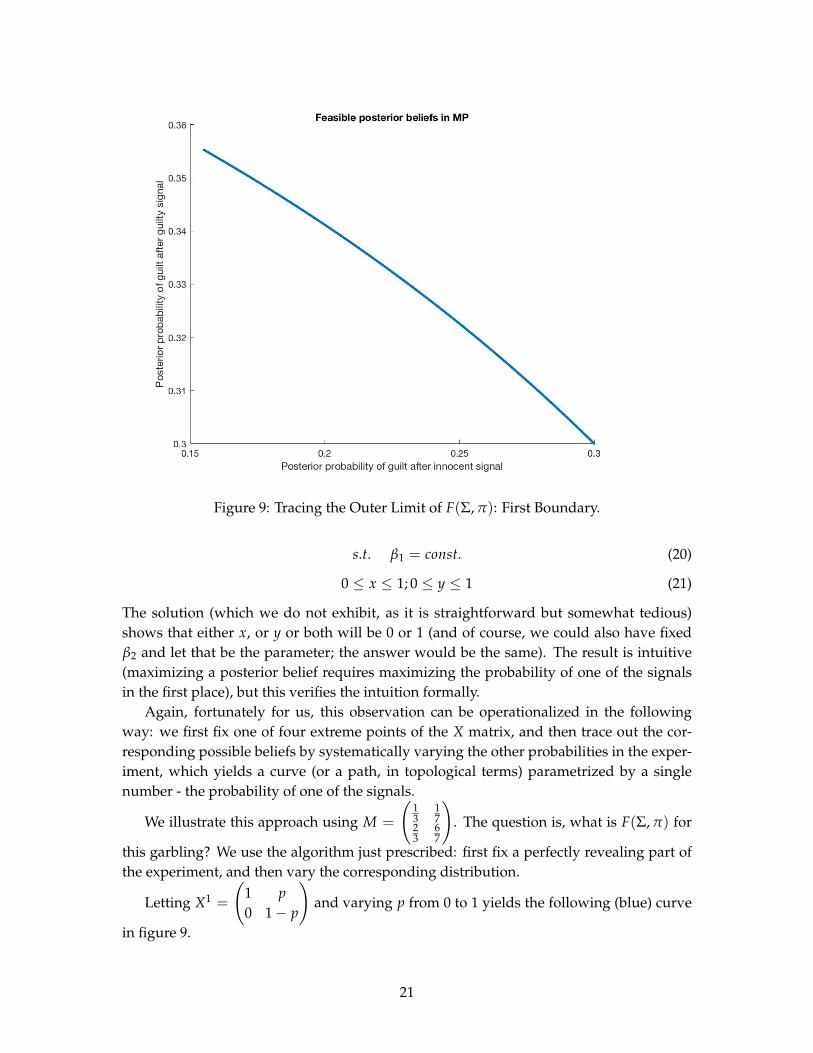
Figure 9: Tracing the Outer Limit of F(Σ, π): First Boundary.

s.t. β1 = const. (20)

0 ≤ x ≤ 1; 0 ≤ y ≤ 1 (21)

The solution (which we do not exhibit, as it is straightforward but somewhat tedious)shows that either x, or y or both will be 0 or 1 (and of course, we could also have fixedβ2 and let that be the parameter; the answer would be the same). The result is intuitive(maximizing a posterior belief requires maximizing the probability of one of the signalsin the first place), but this verifies the intuition formally.

Again, fortunately for us, this observation can be operationalized in the followingway: we first fix one of four extreme points of the X matrix, and then trace out the cor-responding possible beliefs by systematically varying the other probabilities in the exper-iment, which yields a curve (or a path, in topological terms) parametrized by a singlenumber - the probability of one of the signals.

We illustrate this approach using M =

(13

17

23

67

). The question is, what is F(Σ, π) for

this garbling? We use the algorithm just prescribed: first fix a perfectly revealing part ofthe experiment, and then vary the corresponding distribution.

Letting X1 =

(1 p0 1− p

)and varying p from 0 to 1 yields the following (blue) curve

in figure 9.

21

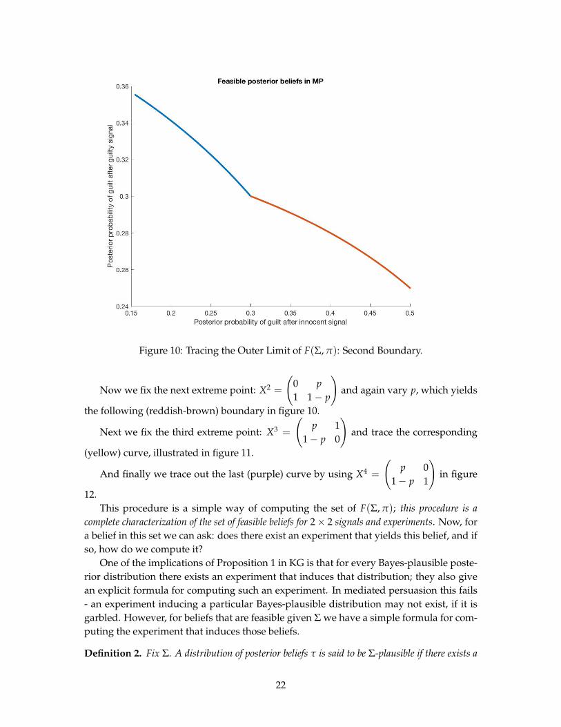
Figure 10: Tracing the Outer Limit of F(Σ, π): Second Boundary.

Now we fix the next extreme point: X2 =

(0 p1 1− p

)and again vary p, which yields

the following (reddish-brown) boundary in figure 10.

Next we fix the third extreme point: X3 =

(p 1

1− p 0

)and trace the corresponding

(yellow) curve, illustrated in figure 11.

And finally we trace out the last (purple) curve by using X4 =

(p 0

1− p 1

)in figure

12.This procedure is a simple way of computing the set of F(Σ, π); this procedure is a

complete characterization of the set of feasible beliefs for 2× 2 signals and experiments. Now, fora belief in this set we can ask: does there exist an experiment that yields this belief, and ifso, how do we compute it?

One of the implications of Proposition 1 in KG is that for every Bayes-plausible poste-rior distribution there exists an experiment that induces that distribution; they also givean explicit formula for computing such an experiment. In mediated persuasion this fails- an experiment inducing a particular Bayes-plausible distribution may not exist, if it isgarbled. However, for beliefs that are feasible given Σ we have a simple formula for com-puting the experiment that induces those beliefs.

Definition 2. Fix Σ. A distribution of posterior beliefs τ is said to be Σ-plausible if there exists a

22

Figure 11: Tracing the Outer Limit of F(Sigma, π): Third Boundary.

Figure 12: Tracing the Outer Limit of F(Σ, π): Fourth Boundary.

23

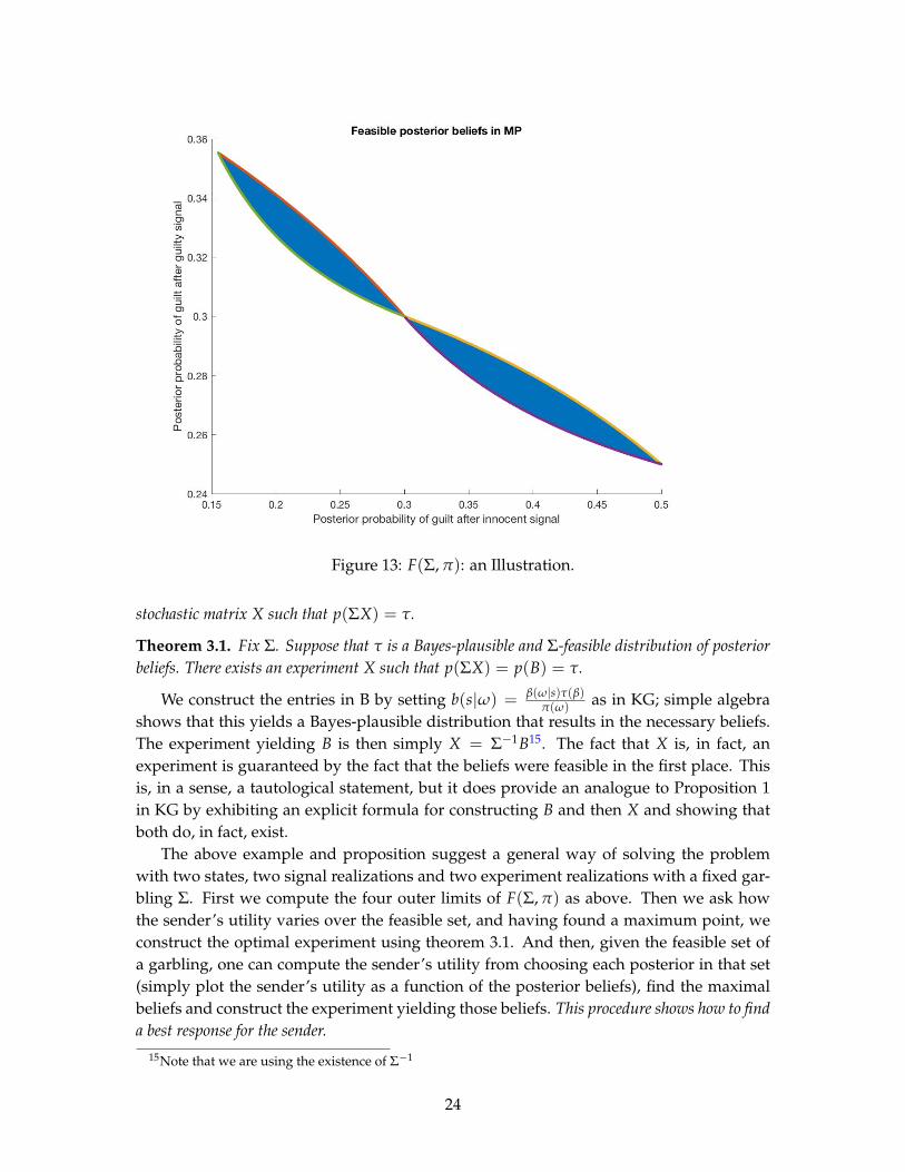
Figure 13: F(Σ, π): an Illustration.

stochastic matrix X such that p(ΣX) = τ.

Theorem 3.1. Fix Σ. Suppose that τ is a Bayes-plausible and Σ-feasible distribution of posteriorbeliefs. There exists an experiment X such that p(ΣX) = p(B) = τ.

We construct the entries in B by setting b(s|ω) = β(ω|s)τ(β)π(ω)

as in KG; simple algebrashows that this yields a Bayes-plausible distribution that results in the necessary beliefs.The experiment yielding B is then simply X = Σ−1B15. The fact that X is, in fact, anexperiment is guaranteed by the fact that the beliefs were feasible in the first place. Thisis, in a sense, a tautological statement, but it does provide an analogue to Proposition 1in KG by exhibiting an explicit formula for constructing B and then X and showing thatboth do, in fact, exist.

The above example and proposition suggest a general way of solving the problemwith two states, two signal realizations and two experiment realizations with a fixed gar-bling Σ. First we compute the four outer limits of F(Σ, π) as above. Then we ask howthe sender’s utility varies over the feasible set, and having found a maximum point, weconstruct the optimal experiment using theorem 3.1. And then, given the feasible set ofa garbling, one can compute the sender’s utility from choosing each posterior in that set(simply plot the sender’s utility as a function of the posterior beliefs), find the maximalbeliefs and construct the experiment yielding those beliefs. This procedure shows how to finda best response for the sender.

15Note that we are using the existence of Σ−1

24

Σ =

( 23

14

13

34

)

Figure 14: Major Features of the Feasible Set

We can write this problem and its solution more formally, which we do now. Let κ bethe constant and denote the maximization program by P. Suppose that the program has asolution16 and denote by x∗(σ1, σ2, π, κ) the solution. Suppose for now that κ ≤ π. Thisproduces a (second posterior belief) function βmax

2 (y; x∗(σ1, σ2, π, κ), σ1, σ2, π) : [0, 1] →[0, 1] we write it to emphasize that all arguments of the βmax

2 function after the semicolonare parameters, and only the y argument is varying from 0 to 1. Analogously we cancompute βmin

2 (y; x∗(σ1, σ2, π, κ), σ1, σ2, π) : [0, 1]→ [0, 1]. Let Gr(βmax2 ) and Gr(βmin

2 ) be thegraphs of the two functions, and let Co(A) be the convex hull of an arbitrary nonemptyset A. We then define F1(Σ, π) , Co(Gr(βmax

2 ) ∪ Gr(βmin2 )); the reason that we can do

that is that we have the set of posterior beliefs is convex (because the set of informationstructures is convex, and Bayes rule is monotonic). Similarly, for κ ≥ π we can computeanalogous objects, and define F2(Σ, π). Finally, we let F(Σ, π) , F1(Σ, π) ∪ F2(Σ, π).

There are a number of important and interesting observations about the Σ-feasibleset that we can make at this point. Consider the F set illustrated in figure 11, using the

garbling matrix

(23

14

13

34

). In this set each point corresponds to an experiment for the

16This amounts to assuming that the κ can actually be a posterior belief, which is not always the case - takefor example the belief β1 = 0.9 in figure 6. Such a belief is clearly infeasible for that Σ, and thus the programwould not have a solution.

25

sender. The first thing to notice is that the so-called ”butterfly” has two ”wings”. The”left” wing - the one including point A, i.e. the wing up and to the left from the ”origin”(i.e. the point where the posteriors are equal to the prior), is the set that would result ifthe sender were using ”natural” signals - i.e. a guilty signal is more likely in the guiltystate and an innocent signal is more likely in the innocent state. The right wing is the setthat would result if the sender were instead using ”perverse” signals - a guilty signal thatis more likely in the innocent state, and vice versa.17 This is also equivalent to flipping thelabels on the signals.

Consider point B, the point where both posteriors are equal to the prior (with theobvious motivation, we call that the ”origin”). Observe that moving weakly northwestmeaning decreasing the first posterior while increasing the second - in other words, amean-preserving spread.18 Thus, points that are northwest of B are posteriors that areBlackwell-more informative than B. Equivalently, they correspond to signals that Black-well dominate the uninformative signals. Iterating this, point A is Blackwell-most in-formative among all the points in the left wing. It can also be verified that point A isprecisely the two posteriors that correspond to the sender using the fully informative (and”natural”) signal. The exact opposite logic applies to the right wing, so that C is the ex-treme posterior corresponding to the Blackwell-most informative ”perverse” signal. Im-portantly, this logic works only within each wing, (or quadrant by quadrant, which aredelineated by the dashed lines), and not on the figure as a whole.

The other observation that we can make is that while F seems symmetric around the”origin”, in general, it is not. The lack of symmetry comes from the constraints (andbiases) imparted by the garbling; F(M, π) is symmetric if and only if M is symmetric.

Definition 3. F is said to be symmetric if for each β1, β2 if the ordered pair β1, β2 ∈ F thenthe ordered pair β2, β1 is also in F.

The next observation is that each wing of the butterfly is convex, but the butterfly itselfis not. This comes from the fact that for normal (and respectively, for perverse) signals, iftwo posteriors can be induced, than so can any convex combination (since the set of therelevant stochastic matrices is convex). On the other hand, for the entire set to be convex,taking a point from the left wing, a point from the right and requiring that a mixturewould also be in the set would require each signal to be weakly more likely in either state- which is impossible, except for the degenerate case. This is why we can take the convexhull of the extreme beliefs and outer limits for each wing, but not the convex hull of theentire butterfly.

The final observation that we can make is the following: the sender is certainly capableof choosing the identity experiment, and inducing ΣI = B (in figure 14 this would corre-spond to point A); this is the best (in the sense of being Blackwell-maximal) that the sendercan induce. Since the sender can also choose any less informative experiment, it wouldseem that the sender may be capable of inducing any Blackwell-inferior distribution to A.

17Note that if the sender were to choose a signal, say, guilty, that is more likely in both states, that wouldquickly bring beliefs back to the prior, and whether it would be in the right or the left wing would be dictatedby the relative probabilities.

18The fact that the spread is mean preserving comes from Bayes rule.

26

Figure 11 shows that this intuition is false. A point like D is certainly Blackwell-inferior toA, being a mean-preserving contraction, yet it is outside the feasible set. The question thenarises, why can we not simply ”construct” the required experiment X as follows: supposeΣI B ′ and p(B ′) = D. If there exists an X with ΣX = B ′, we would be done. Whatabout simply putting X = Σ−1B ′? The answer is that if p(ΣΣ−1B ′) is in F, this wouldwork. It turns out that if that it not true, then Σ−1B ′ will not yield a stochastic matrix Xand therefore would not be a valid experiment (this can be seen by example). In otherwords, the sender is not capable of inducing any posterior belief that is Blackwell-inferiorto ΣI.

There are a number of interesting results that we can illustrate using this techniqueof characterizing the feasible sets. To give but one example, we give a simple proof ofa result first described in Bohnenblust, Shapley and Sherman (1949), and alluded to inBlackwell’s original work (Blackwell (1951), Blackwell (1953)):

Theorem 3.2. Suppose Σ1 and Σ2 are two garblings with Σ1 B Σ2. Then F(Σ2, π) ⊆ F(Σ1, π).

Proof. Fix any π. We must show that for any τ if supp(τ) ∈ F(Σ2, π), then supp(τ) ∈F(Σ1, π). By assumption we have that p(Σ2X) = τ for some X. The question is, doesthere exist a Y such that τ = p(Σ1Y)? In other words, does there exist a Y such thatΣ2X = Σ1Y? The answer is yes; by assumption we have that ΓΣ1 = Σ2 for some Γ. Thus,

Σ2X = Σ1Y ⇒ ΓΣ1X = Σ1Y (22)

and therefore the required Y is given by

Y = Σ−11 ΓΣ1X (23)

Note that Y does depend on both Σ1 and X, as intuition would suggest.

In other words, using a strictly more Blackwell-informative garbling results in a strictlylarger set of feasible receiver posterior beliefs. Of course, this is obvious with trivialgarblings (an identity, which would leave the feasible set unchanged from the Bayes-plausible one, and a completely uninformative garbling which would reduce the set toa single point - just the prior), but this theorem shows that the same ”nesting” is true fornontrivial Blackwell-ranked garblings.

We illustrate (see figure 15) this observation using Σ1 =

(910

1100

110

99100

)and Σ2 =

(23

14

13

34

);

it can be readily checked that Σ1 B Σ2.With ”filled in” convex hulls the same idea is represented in figure 16.Similarly, if Σ1 and Σ2 are not ranked by Blackwell’s criterion, the F sets are not nested.

We illustrate this by an example: consider Σ1 =

(23

13

13

23

)and Σ2 =

(45

12

15

12

).19 The F sets

are illustrated in figure 17.

19It can be readily checked that these matrices are not ranked.

27

Figure 15: Blackwell’s Order Implies Set Inclusion for Feasible Sets.

Figure 16: Further Illustration of Set Inclusion.

28

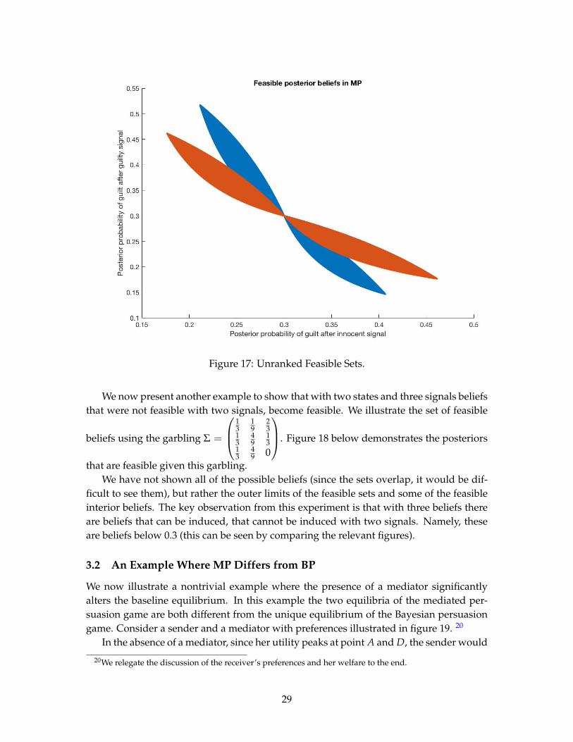
Figure 17: Unranked Feasible Sets.

We now present another example to show that with two states and three signals beliefsthat were not feasible with two signals, become feasible. We illustrate the set of feasible

beliefs using the garbling Σ =

13

19

23

13

49

13

13

49 0

. Figure 18 below demonstrates the posteriors

that are feasible given this garbling.We have not shown all of the possible beliefs (since the sets overlap, it would be dif-

ficult to see them), but rather the outer limits of the feasible sets and some of the feasibleinterior beliefs. The key observation from this experiment is that with three beliefs thereare beliefs that can be induced, that cannot be induced with two signals. Namely, theseare beliefs below 0.3 (this can be seen by comparing the relevant figures).

3.2 An Example Where MP Differs from BP

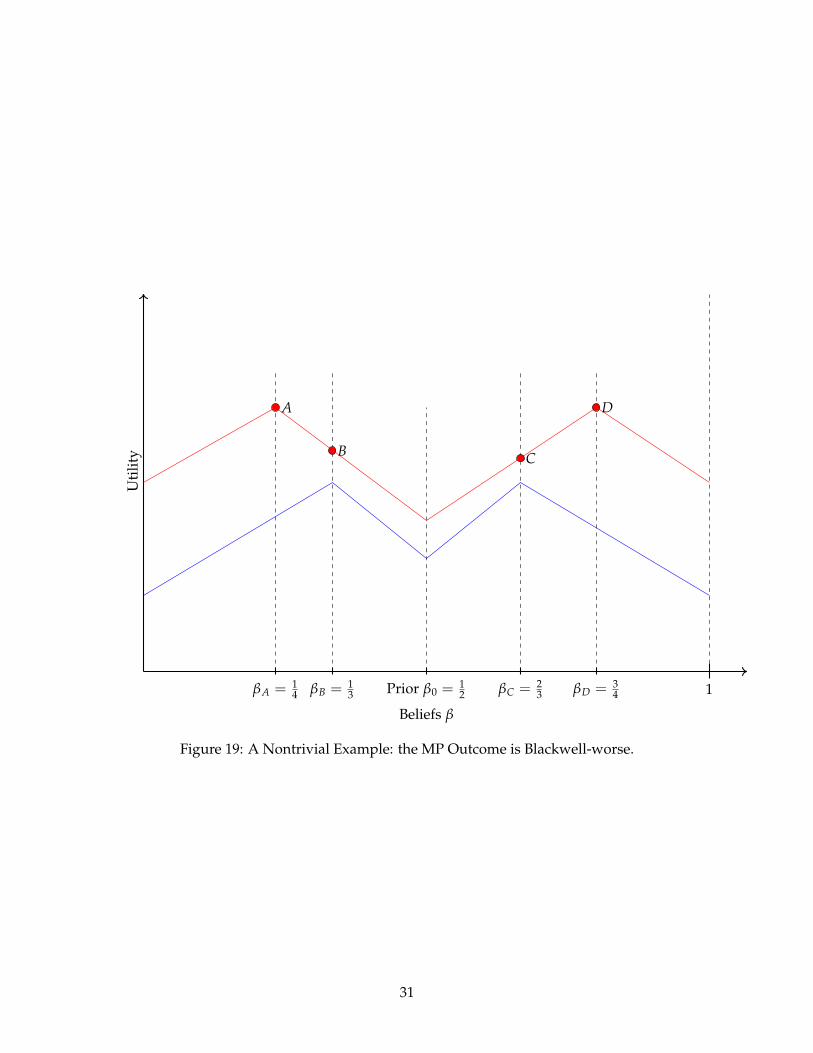
We now illustrate a nontrivial example where the presence of a mediator significantlyalters the baseline equilibrium. In this example the two equilibria of the mediated per-suasion game are both different from the unique equilibrium of the Bayesian persuasiongame. Consider a sender and a mediator with preferences illustrated in figure 19. 20

In the absence of a mediator, since her utility peaks at point A and D, the sender would

20We relegate the discussion of the receiver’s preferences and her welfare to the end.

29

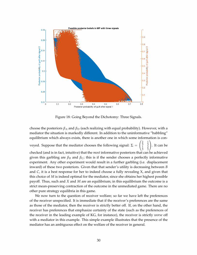
Figure 18: Going Beyond the Dichotomy: Three Signals.

choose the posteriors βA and βD (each realizing with equal probability). However, with amediator the situation is markedly different. In addition to the uninformative ”babbling”equilibrium which always exists, there is another one in which some information is con-

veyed. Suppose that the mediator chooses the following signal: Σ =

(23

13

13

23

). It can be

checked (and is in fact, intuitive) that the most informative posteriors that can be achievedgiven this garbling are βB and βC; this is if the sender chooses a perfectly informativeexperiment. Any other experiment would result in a further garbling (i.e. displacementinward) of these two posteriors. Given that that sender’s utility is decreasing between Band C, it is a best response for her to indeed choose a fully revealing X, and given thatthis choice of M is indeed optimal for the mediator, since she obtains her highest possiblepayoff. Thus, such and X and M are an equilibrium; in this equilibrium the outcome is astrict mean-preserving contraction of the outcome in the unmediated game. There are noother pure strategy equilibria in this game.

We now turn to the question of receiver welfare; so far we have left the preferencesof the receiver unspecified. It is immediate that if the receiver’s preferences are the sameas those of the mediator, then the receiver is strictly better off. If, on the other hand, thereceiver has preferences that emphasize certainty of the state (such as the preferences ofthe receiver in the leading example of KG, for instance), the receiver is strictly worse offwith a mediator in this example. This simple example illustrates that the presence of themediator has an ambiguous effect on the welfare of the receiver in general.

30

1Prior β0 = 12

Beliefs β

Uti

lity

βA = 14 βD = 3

4βB = 13 βC = 2

3

A

B

D

C

Figure 19: A Nontrivial Example: the MP Outcome is Blackwell-worse.

31

3.3 Comparing Equilibrium Outcomes

We finally come to the main part of the paper - evaluating the effect of adding a media-tor to a Bayesian persuasion environment. There are a few general21 results that we canobtain when comparing outcomes with and without a mediator. Indeed, with a mediator,there is always a babbling equilibrium. Thus, even when there may be nontrivial per-suasion/information revelation in the BP problem, there is an equilibrium without anyinformation revelation in the MP problem, even though the preferences of the sender andthe receiver are the same across the two problems. The second general result is that if weadd a mediator whose utility is, say, globally strictly concave22 over the set of posteriors,not only does a babbling equilibrium exists, but it is unique.

If sender’s utility is globally strictly concave, the unique outcome in both games is norevelation. If the sender’s utility is globally strictly convex, the unique outcome in bothgames is full revelation. If both the sender’s and the mediator’s utilities are linear, thenany outcome can be sustained in equilibrium.

At this point, to be able to say more about outcomes, we need to start narrowingdown the scope of utilities. Toward this end, suppose that the receiver’s utility is convex(or at least piece-wise convex), and the sender benefits from persuasion (in the languageof Kamenica and Gentzkow (2011)). The first result that we can state has to do withcomparing two MP games where the preferences of the mediator are different; namelythe set of outcomes when uM = uR is a subset of the set of equilibrium outcomes whenuM = uS.

We now turn to comparing the informativeness of MP outcomes relative to BP out-comes and show by example that it is possible for an equilibrium of the MP game to bestrictly more informative in the Blackwell sense than the equilibrium of the BP game.

Consider a sender and a mediator with preferences that are illustrated in figure 20; inthis figure the sender’s utility is in red and that of the mediator is in blue. The sender’sutility vanishes for beliefs below 0.2, then jumps up at 0.2, jumps back down to a valueof −k, for k positive and ”large”, for beliefs β ∈ (0.2, 0.955), except for another jump upat 0.5 then jumps up at 0.955, and then returns to 0. The mediator’s utility is M-shapedand peaks at 0.17 and 0.955. The common prior is β0; without a mediator the senderwould clearly choose the posteriors βBP

1 , βBP2 = 0.2, 0.5. They are certainly Bayes-

plausible, and give the sender her highest possible utility. Suppose however that the

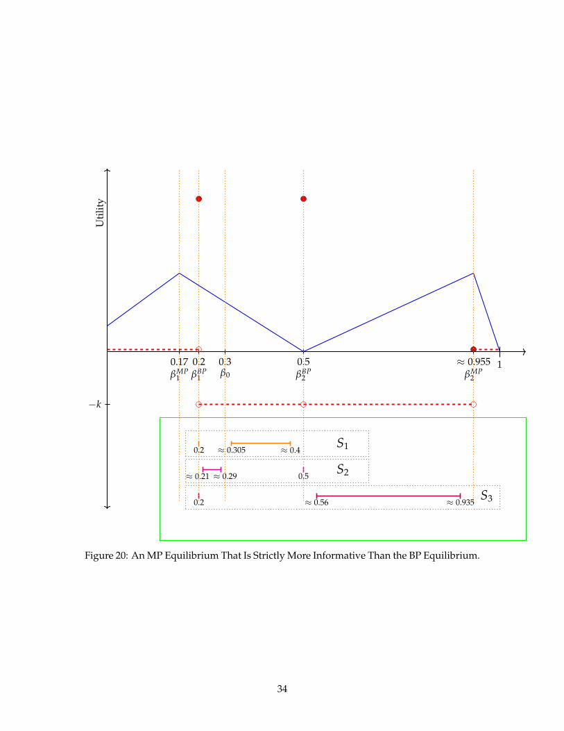
mediator chose to play the following garbling: Σ =

(12

1100

12

99100

); the F(Σ, 0.3) set for this

garbling is depicted in blue in figure 19. If the sender were to simultaneously play a fullyrevealing experiment, the outcome would be βMP

1 , βMP2 = 0.17, 0.955, yielding her

a payoff of 0; note also that this is the most preferred outcome of the mediator. Giventhis garbling, the only way in which the sender can improve her payoff is by deviating tosomething that induces a posterior of 0.2, or 0.5. Suppose she deviates to something thatresults in one posterior (say, the first one) begin βdeviation

1 = 0.2. Then the second posterior

21I.e. those that do not depend on the exact form of the utility functions.22Versions of this result that involve the mediator’s utility being concave over some set of posteriors, or not

being strictly concave are analogous and straightforward enough; we do not state them.

32

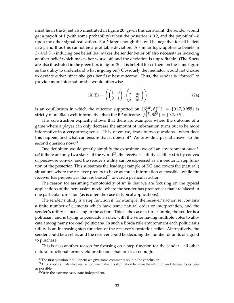
must lie in the S1 set also illustrated in figure 20; given this constraint, the sender wouldget a payoff of 1 (with some probability) when the posterior is 0.2, and the payoff of −kupon the other signal realization. For k large enough this will be negative for all beliefsin S1, and thus this cannot be a profitable deviation. A similar logic applies to beliefs inS2 and S3 - inducing one belief that makes the sender better off also necessitates inducinganother belief which makes her worse off, and the deviation is unprofitable. (The S setsare also illustrated in the green box in figure 20; it is helpful to see them on the same figureas the utility to understand what is going on.) Obviously the mediator would not chooseto deviate either, since she gets her first best outcome. Thus, the sender is ”forced” toprovide more information she would otherwise

(X, Σ) =

((1 00 1

),

(12

1100

12

99100

))(24)

is an equilibrium in which the outcome supported on βMP1 , βMP

2 = 0.17, 0.955 isstrictly more Blackwell-informative than the BP outcome βBP

1 , βBP2 = 0.2, 0.5.

This construction explicitly shows that there are examples where the outcome of agame where a player can only decrease the amount of information turns out to be moreinformative in a very strong sense. This, of course, leads to two questions - when doesthis happen, and what can ensure that it does not? We provide a partial answer to thesecond question now.23

One definition would greatly simplify the exposition; we call an environment canoni-cal if there are only two states of the world24, the receiver’s utility is either strictly convexor piecewise convex, and the sender’s utility can be expressed as a monotonic step func-tion of the posterior. This subsumes the leading example of KG and covers the (natural!)situations where the receiver prefers to have as much information as possible, while thereceiver has preferences that are biased25 toward a particular action.

The reason for assuming monotonicity of uS is that we are focusing on the typicalapplications of the persuasion model where the sender has preferences that are biased inone particular direction (as is often the case in typical applications).

The sender’s utility is a step function if, for example, the receiver’s action set containsa finite number of elements which have some natural order or interpretation, and thesender’s utility is increasing in the action. This is the case if, for example, the sender is apolitician, and is trying to persuade a voter, with the voter having multiple votes to allo-cate among many (or one) politicians. In such a Borda rule environment each politician’sutility is an increasing step function of the receiver’s posterior belief. Alternatively, thesender could be a seller, and the receiver could be deciding the number of units of a goodto purchase.

This is also another reason for focusing on a step function for the sender - all othernatural functional forms yield predictions that are clear enough.

23The first question is still open; we give some comments on it in the conclusion.24This is not a substantive restriction; we make this stipulation to make the intuition and the results as clear

as possible.25Or in the extreme case, state-independent.

33

1β0βBP

1 βBP2

0.2 0.3 0.5βMP

1

0.17βMP

2

≈ 0.955

−k

Uti

lity

S1

S2

S3

0.2 ≈ 0.305 ≈ 0.4

0.5≈ 0.21 ≈ 0.29

0.2 ≈ 0.56 ≈ 0.935

Figure 20: An MP Equilibrium That Is Strictly More Informative Than the BP Equilibrium.

34

Σ =

( 12

1100

12

99100

)

S1

S3S2

Figure 21: Feasible set F(Σ, 0.3)

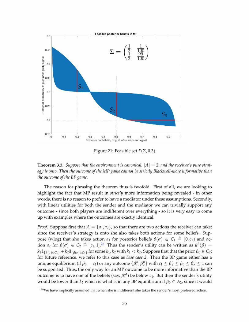
Theorem 3.3. Suppose that the environment is canonical, |A| = 2, and the receiver’s pure strat-egy is onto. Then the outcome of the MP game cannot be strictly Blackwell-more informative thanthe outcome of the BP game.

The reason for phrasing the theorem thus is twofold. First of all, we are looking tohighlight the fact that MP result in strictly more information being revealed - in otherwords, there is no reason to prefer to have a mediator under these assumptions. Secondly,with linear utilities for both the sender and the mediator we can trivially support anyoutcome - since both players are indifferent over everything - so it is very easy to comeup with examples where the outcomes are exactly identical.

Proof. Suppose first that A = a1, a2, so that there are two actions the receiver can take;since the receiver’s strategy is onto she also takes both actions for some beliefs. Sup-pose (wlog) that she takes action a1 for posterior beliefs β(σ) ∈ C1 , [0, c1) and ac-tion a2 for β(σ) ∈ C2 , [c1, 1].26 Thus the sender’s utility can be written as uS(β) =

k11β(σ)∈C1+ k21β(σ)∈C2 for some k1, k2 with k1 < k2. Suppose first that the prior β0 ∈ C2;for future reference, we refer to this case as base case 2. Then the BP game either has aunique equilibrium (if β0 = c1) or any outcome βB

1 , βB2 with c1 ≤ βB

1 ≤ β0 ≤ βB2 ≤ 1 can

be supported. Thus, the only way for an MP outcome to be more informative than the BPoutcome is to have one of the beliefs (say, βM

1 ) be below c1. But then the sender’s utilitywould be lower than k2 which is what is in any BP equilibrium if β0 ∈ A2, since it would

26We have implicitly assumed that when she is indifferent she takes the sender’s most preferred action.

35

Σ =

( 67

37

17

47

)βB1 , βB

2 =

13 , 2

3

βM1 , βM

2 = 1

3 , 45

Figure 22: An Informative MP Equilibrium in a Canonical Environment.

36

have to be some combination of k1 and k2 and k1 < k2 by monotonicity. Therefore therealways exists a profitable deviation for the sender - choose an uninformative experiment,and bring the utility back up to k2; this is always feasible and is strictly better so in thiscase an MP outcome cannot be strictly more informative than the BP outcome.

Suppose now that β0 ∈ C1 \ 0; for future reference, we refer to this case as base case1. Note that in this case there is a unique equilibrium in the BP game:βB

1 , βB2 = 0, c1.27

The only way for an MP outcome to be more informative is to have βM2 > c1.28; denote

by X∗, Σ∗ the choices leading to such an outcome. But then we would have 0, c1 /∈F(Σ∗, β0) and yet 0, βM

2 ∈ F(Σ∗, β0). Direct computation (which we omit) shows thatthis is impossible. Finally, if β0 = 0, i.e. the prior vanishes to begin with, then the onlyBayes-plausible posteriors are uninformative in both the BP and the MP cases, and thus,one cannot be strictly more informative than the other. This finishes the proof for the casewhere |A| = 2.

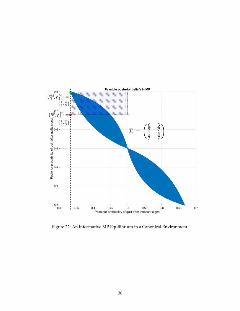
We now show by example that even in this simple and canonical setting the MP out-come can be strictly more informative than the BP outcome. Suppose that the commonprior is β0 = 1

2 , that A = a1, a2, a3, and that the optimal strategy of the receiver is totake action a1 for β(σ) ∈ [0, 1

3 ), take action a2 for β(σ) ∈ [ 13 , 2

3 ), and take action a3 forβ(σ) ∈ [ 2

3 , 1]. By monotonicity of the sender’s utility it follows that she would induce

posterior beliefs τBP =

13 with probability 1

223 with probability 1

2

, using the experiment XBP =

(23

13

13

23

).

We claim, however, that with the appropriate preferences for the mediator, the pairX∗, Σ∗ can be an equilibrium, where

X∗ =

(1 00 1

), Σ∗ =

(67

37

17

47

)(25)

yielding the following distribution of posterior beliefs: τMP =

13 with probability 9

1445 with probability 5

14

.

It can be checked (and is in fact, graphically apparent from figure 22) that τMP is a mean-preserving spread of τBP, so that the MP outcome is Blackwell more informative than theBP outcome. To show that this is an equilibrium, we check that nobody can profitablydeviate. Suppose first that the mediator is choosing Σ∗; F(Σ∗, 1

2 ) is depicted in figure 22.In the shaded region the sender’s utility is increasing in the southwestern direction, so fork3 high enough the best that she could do is induce the green point (using a fully revealinginformation structure). And given that the sender is choosing full revelation, it is easy toconstruct mediator preferences that would result in Σ∗ being the optimal choice.

We say that the receiver benefits from mediation if the receiver’s utility in the mediatedpersuasion game is strictly greater than her utility in the Bayesian persuasion game, whereof course we compare games where the preferences of the sender and the receiver do not

27Note also that in this case after one of the signal realizations the receiver will take a worst action for thesender, and thus, by a theorem from KG, she will be certain of her action in that case.

28Of course, we also have βM1 = 0.

37

change between games.We now show a surprising result; when the preferences of the mediator are perfectly

aligned with those of the sender (or alternatively, the receiver simply is the mediator), thereceiver cannot benefit from mediation. The import of this finding is that the receiver ben-efits from mediation when the mediator’s preferences are such that the mediator prefersmore information revelation, in the sense of Blackwell, than the sender, but less infor-mation revelation than the receiver (which in a canonical environment, is of course, fullrevelation).

Theorem 3.4. Suppose that the environment is canonical, and furthermore that uM = uR; sup-pose to avoid trivialities that the sender also benefits from persuasion. We now show that if τ∗ withsupport equal to β∗1, β∗2 is an equilibrium outcome, then we cannot have τ∗ τBP.

Proof. Suppose, towards a contradiction, that τ∗ τBP, and denote by (X∗, Σ∗) the in-formation structures chosen. By supposition, Σ 6= I2, since otherwise we would haveβ∗1, β∗2 = βBP

1 , βBP2 ; so the mediator must be choosing some nontrivial garbling. Note

that this also implies that X∗ XBP. Thus, since the mediator’s utility is convex, devi-ating to Σ ′ = I2 yields a strictly higher utility, and thus, (X∗, Σ∗) could not have been anequilibrium.

In other words, if uM = uR, the receiver cannot strictly benefit since if that were thecase, the mediator would have a profitable deviation. And that profitable deviation - nogarbling at all - cannot be part of an equilibrium where τ∗ τBP since then the senderwould have a profitable deviation, bringing beliefs back to the BP outcome, which mustnow be feasible, since the mediator is not garbling the information at all, and thus allBayes-plausible beliefs are feasible. Thus, if the sender were the mediator, there can exista garbling that makes her better off, but that cannot be an equilibrium, since there is alsoalways a better one still until we get to no garbling at all, which again cannot be part of anequilibrium. In fact, remarkably enough, it can be shown that the outcome when uM = uR

is either uninformative (i.e. β∗1 = β∗2 = β0), or it coincides with the BP outcome29. In otherwords, in the dichotomy setting, the nontrivial outcome when uM = uS or when uM = uR

is exactly the same.We have established two important points: 1) the receiver can be better off in a very

strong sense with a mediator, even though the mediator can only destroy information, and2) for this to happen the preferences of the mediator cannot be the same as the preferencesof the receiver (or the sender, for that matter). It must be the case that the mediator prefersmore information revelation than the sender, but not perfect revelation (which of courseis the preferred outcome of the receiver by assumption).

29The argument is simple and goes like this - we have shown that we cannot have τ∗ τBP strictly; we alsocannot have τBP τ∗ since then the mediator would have a profitable deviation. Finally, if the posteriorswere unranked, the mediator would again move one of the beliefs outward until it at least coincides with theBP belief. This exhausts the possibilities and proves the result.

38

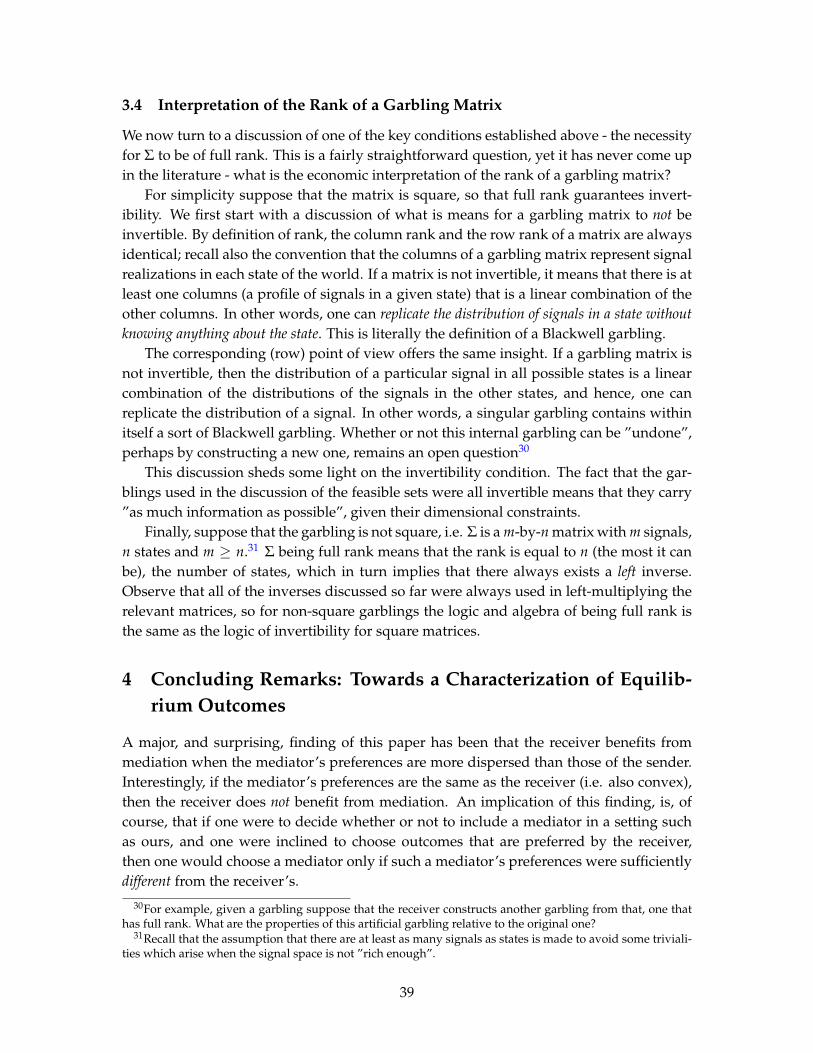
3.4 Interpretation of the Rank of a Garbling Matrix

We now turn to a discussion of one of the key conditions established above - the necessityfor Σ to be of full rank. This is a fairly straightforward question, yet it has never come upin the literature - what is the economic interpretation of the rank of a garbling matrix?

For simplicity suppose that the matrix is square, so that full rank guarantees invert-ibility. We first start with a discussion of what is means for a garbling matrix to not beinvertible. By definition of rank, the column rank and the row rank of a matrix are alwaysidentical; recall also the convention that the columns of a garbling matrix represent signalrealizations in each state of the world. If a matrix is not invertible, it means that there is atleast one columns (a profile of signals in a given state) that is a linear combination of theother columns. In other words, one can replicate the distribution of signals in a state withoutknowing anything about the state. This is literally the definition of a Blackwell garbling.

The corresponding (row) point of view offers the same insight. If a garbling matrix isnot invertible, then the distribution of a particular signal in all possible states is a linearcombination of the distributions of the signals in the other states, and hence, one canreplicate the distribution of a signal. In other words, a singular garbling contains withinitself a sort of Blackwell garbling. Whether or not this internal garbling can be ”undone”,perhaps by constructing a new one, remains an open question30

This discussion sheds some light on the invertibility condition. The fact that the gar-blings used in the discussion of the feasible sets were all invertible means that they carry”as much information as possible”, given their dimensional constraints.

Finally, suppose that the garbling is not square, i.e. Σ is a m-by-n matrix with m signals,n states and m ≥ n.31 Σ being full rank means that the rank is equal to n (the most it canbe), the number of states, which in turn implies that there always exists a left inverse.Observe that all of the inverses discussed so far were always used in left-multiplying therelevant matrices, so for non-square garblings the logic and algebra of being full rank isthe same as the logic of invertibility for square matrices.

4 Concluding Remarks: Towards a Characterization of Equilib-rium Outcomes

A major, and surprising, finding of this paper has been that the receiver benefits frommediation when the mediator’s preferences are more dispersed than those of the sender.Interestingly, if the mediator’s preferences are the same as the receiver (i.e. also convex),then the receiver does not benefit from mediation. An implication of this finding, is, ofcourse, that if one were to decide whether or not to include a mediator in a setting suchas ours, and one were inclined to choose outcomes that are preferred by the receiver,then one would choose a mediator only if such a mediator’s preferences were sufficientlydifferent from the receiver’s.

30For example, given a garbling suppose that the receiver constructs another garbling from that, one thathas full rank. What are the properties of this artificial garbling relative to the original one?

31Recall that the assumption that there are at least as many signals as states is made to avoid some triviali-ties which arise when the signal space is not ”rich enough”.

39

We now comment informally on what a characterization equilibrium outcomes mightlook like. The first observation that one can make is that if a belief is part of an equilibriumoutcome, it must be the case that at that belief the utility of a player coincides with theconcavification of the utility; Matthew Gentzkow and Emir Kamenica refer to such beliefsas ”coincident” throughout their work on this topic. This narrows down the set of possiblebeliefs considerably.

The second important observation is that if there is to be any information revelation,the utilities of the players have to be convex over a set that includes the prior. Let us call aset of posterior beliefs of a player a convex basin if is the set over which the utility is weaklyconvex. Putting these two observations together, we obtain a hint of what characterizationof equilibrium outcomes might look like - it must be the intersection of convex basins32 ofplayers’ utilities, and a belief can be part of an equilibrium outcome only if is coincidentover this intersection of convex basins. While a formal statement is not available at themoment, it seems to be within our grasp.

The future of this project will address sequential versions of this model - namely, whathappens when we allow the mediator to move before or after the sender, and perhaps,condition the mediator’s choice of action upon the experiment chosen by the sender, whilestill maintaining the assumption of fixed signal realization spaces. In other words, wewill work on understanding sequential persuasion where players can also destroy infor-mation, not only add it, as has been the case up to now.

32Or at least a union of convex basins, to account for the possibility of an inverse-M-shaped utility function.

40

References

[1] Alonso, Ricardo and Odilon Camara. (2016). ”Bayesian Persuasion with Heteroge-neous Priors.” Journal of Economic Theory, Volume 165, 2016, Pages 672-706, ISSN0022-0531, http://dx.doi.org/10.1016/j.jet.2016.07.006.

[2] Ambrus, A., Azevedo, E. M. and Kamada, Y. (2013). ”Hierarchical Cheap Talk.” The-oretical Economics, 8: 233-261. doi:10.3982/TE1038

[3] Aumann, Robert and Michael Maschler. (1995). Repeated Games with Incomplete Infor-mation. The MIT Press.

[4] Ben-Porath, Elchanan and Dekel, Eddie. (1992). ”Signaling Future Actions and thePotential for Sacrifice”. Journal of Economic Theory, 57, issue 1, p. 36-51.

[5] Blackwell, David. (1951). ”Comparison of Experiments.” Proceedings of the SecondBerkeley Symposium on Mathematical Statistics and Probability, 93-102, University ofCalifornia Press, Berkeley, Calif.

[6] Blackwell, David. (1953). ”Equivalent Comparisons of Experiments.” Ann. Math.Statist. 24, no. 2, 265-272.

[7] Blume, Andreas, Oliver J. Board and Kohei Kawamura. (2007). ”Noisy Talk.” Theoret-ical Economics, vol. 2, no. 4. pp.395-440.

[8] Blume, Andreas. (2012). ”A class of strategy-correlated equilibria in sender-receivergames.” Games and Economic Behavior, vol. 75. no. 2, pp. 510-517.

[9] Bohnenblust, H.F., L.S. Shapley and S. Sherman. (1949). ”Reconnaissance in GameTheory”. US Air Force Project RAND Research Memorandum 208.

[10] Coval, Joshua D. and Jurek, Jakub W. and Stafford, Erik.(2008). ”The Economicsof Structured Finance.” (October 20, 2008). Harvard Business School Finance Work-ing Paper No. 09-060. Available at SSRN: https://ssrn.com/abstract=1287363 orhttp://dx.doi.org/10.2139/ssrn.1287363

[11] Ely, Jeffrey C. (2017). ”Beeps.” American Economic Review, 107 (1): 31-53.

[12] Geanakoplos, John. (1989). ”Game Theory without Partitions, with Applications toSpeculation and Consensus”. Cowles Foundation Discussion Paper No.914.

[13] Gentzkow, Matthew and Emir Kamenica. (2017a). ”Competition in Persuasion.” Re-view of Economic Studies, vol. 84, no. 4, pp. 300-322.

[14] Gentzkow, Matthew and Emir Kamenica. (2017b). ”Bayesian Persuasion with Mul-tiple Senders and Rich Signal Spaces.” Games and Economic Behavior, Volume 104,Pages 411-429, https://doi.org/10.1016/j.geb.2017.05.004.

[15] Hedlund, Jonas, (2017). ”Bayesian Persuasion by a Privately Informed Sender.” Jour-nal of Economic Theory, 167, issue C, p. 229-268

41

[16] Kamenica, Emir, and Matthew Gentzkow. (2011). ”Bayesian Persuasion.” AmericanEconomic Review, 101(6): 2590-2615.

[17] Kosenko, Andrew. (2018). ”Bayesian Persuasion with Private Information.” Workingpaper. Available at: andrewkosenko.com

[18] Li, Fei and Norman, Peter. ”Sequential Persuasion” Working Paper,(June 15, 2018). Available at SSRN: https://ssrn.com/abstract=2952606 orhttp://dx.doi.org/10.2139/ssrn.2952606

[19] Lipnowski, Elliott, Doron Ravid and Denis Shishkin. (2018). ”Persuasion via WeakInstitutions”. Working paper. Available at SSRN: https://ssrn.com/abstract=3168103or http://dx.doi.org/10.2139/ssrn.3168103

[20] Pollrich, Martin. (2017). ”Mediated audits.” The RAND Journal of Economics, 48:44-68. doi:10.1111/1756-2171.12167

[21] Rahman, David and Ichiro Obara. (2010). ”Mediated Partnerships.” Econometrica,78: 285-308. doi:10.3982/ECTA6131

[22] Rubinstein, Ariel. (1997). Modeling Bounded Rationality. MIT Press, 1997.

[23] Samuelson, Larry. (2004). ”Modeling Knowledge in Economic Analysis,” Journal ofEconomic Literature, vol. 42, pp. 367-403.

[24] Sah, Raaj Kumar, and Joseph E. Stiglitz. (1986). ”The Architecture of Economic Sys-tems: Hierarchies and Polyarchies.” The American Economic Review, vol. 76, no. 4, pp.716-727

[25] Tsakas, Elias and Nicolas Tsakas (2018). ”Noisy Persuasion”. Working paper. Avail-able at http://www.elias-tsakas.com/Research/Papers/NoisyPersuasion.pdf

[26] Le Treust, Mael and Tristan Tomala (2018). ”Persuasion with Limited Communica-tion Capacity”. Working paper. Available at: https://arxiv.org/pdf/1711.04474.pdf

42