Medical Image Communications:Wavelet Based Compression Techniques

Neal Andrew Snooke

Department of Computer ScienceUniversity of Wales

Aberystwyth

September 1994

This thesis is submitted in fulfilment of the requirements for the degree of

Doctor of Philosophy of The University of Wales

Certification

The work presented in this thesis has been carried out under thesupervision of David Price and Nigel Hardy of the Department ofComputer Science, University of Wales, Aberystwyth.

Neal Andrew Snooke

David Price(Supervisor)

Nigel Hardy(Supervisor)

i

Declaration

This thesis has not already been accepted in substance for any de-gree, and is not concurrently submitted in candidature for any de-gree.

Neal Andrew Snooke

Originality is not claimed for all parts of this thesis, where materialfrom published sources is used appropriate acknowledgement ismade both in the text and in the bibliography.

Neal Andrew Snooke

David Price(Supervisor)

Nigel Hardy(Supervisor)

ii

Copyright

I hereby give consent for my thesis, if accepted to be available forphotocopying and for inter-library loans, and for the title and sum-mary to be made available to outside organisations.

Neal Andrew Snooke

iii

Abstract

The work of this thesis is based on an investigation of the potential for utilising theIntegrated Services Digital Network (ISDN) for image transmission within a medical scenario.The work initially identifies the major requirements of the application, and suggests that someform of compression of the data is necessary, with the possibility of progressive enhancementin some situations.

We consider a number of state of the art encoding approaches and provide evaluation ofeach within this context. The approach is taken that the many advantages of lossy encodingoften outweigh the disadvantages, although effective use of these techniques can only be madewhen characteristics of the data redundant to the future use of the image is identified. Sourcesof redundancy are located at several levels, not only visual sensitivity, but from statistical andspatial structure, based on external knowledge about the image and application.

The Wavelet transformation was selected due to a number of very useful characteristicswhich we exploit in the development of a compression scheme capable of supporting boththe statistical and human visual models as well as providing a framework for allowinghigher level regional information to be used to allow non uniform quality selection. Thusthe potential ability to preserve the diagnostic information content of the image which canbe lost with general lossy encoding techniques is sought, whilst still maintaining the highcompression rates characteristic of lossy compression.

The scheme can easily be developed into a high ratio archive algorithm; the implicationsof this use are also considered throughout the work.

iv

Acknowledgements

My Thanks go to the following individuals and organisations for their support and assis-tance during the research and writing of this thesis.

First I should thank my supervisor Dave Price for encouraging me to pursue this researchin the first place, and to Hewlett Packard Ltd for allowing me to leave their graduate schemeto return to Aberystwyth.

Many people have contributed directly or indirectly through discussions, but in particularI must also thank Dr. Horst Holstein for several reviews and useful discussions throughoutthe work.

Thanks to Prof. Mark Lee for reading and commenting on this thesis and also for ‘gentlepersuasion’ to ensure it was submitted on time.

I must thank the SERC (now the EPSRC) who provided my funding during this work, andalso to the FLAME project especially Dr. Chris Price and Dr. Dave Pugh who have been sounderstanding of my needs for time off to complete the final stages of writing up this work.

The time I have spent pursuing this work would surly not have been as pleasurablewithout the staff and research students in the Computer Science department at Aberystwyth.Thank you to everyone else who I have not previously mentioned.

v

To my parents for encouraging meto concentrate on this work

... and to Julie, Beci & Susiefor distracting me.

vi

Contents

1 Introduction 11.1 Background : : : : : : : : : : : : : : : : : : : : : : : : : : : : : : : : : : : : : : 11.2 Outline of objectives : : : : : : : : : : : : : : : : : : : : : : : : : : : : : : : : : 11.3 Structure of the thesis : : : : : : : : : : : : : : : : : : : : : : : : : : : : : : : : 31.4 Integration of disciplines : : : : : : : : : : : : : : : : : : : : : : : : : : : : : : 41.5 Teleworking : : : : : : : : : : : : : : : : : : : : : : : : : : : : : : : : : : : : : 51.6 Medical imaging technology : : : : : : : : : : : : : : : : : : : : : : : : : : : : 51.7 Telemedicine : : : : : : : : : : : : : : : : : : : : : : : : : : : : : : : : : : : : : 61.8 Description of TR services : : : : : : : : : : : : : : : : : : : : : : : : : : : : : : 6

1.8.1 Potential benefits of TR services : : : : : : : : : : : : : : : : : : : : : : 71.9 Image compression technology : : : : : : : : : : : : : : : : : : : : : : : : : : : 81.10 Future applicability : : : : : : : : : : : : : : : : : : : : : : : : : : : : : : : : : 81.11 What this work does not address : : : : : : : : : : : : : : : : : : : : : : : : : : 9

2 Brief History and Review of Recent Work 102.1 Telemedicine: the early days : : : : : : : : : : : : : : : : : : : : : : : : : : : : 10

2.1.1 Digital teleradiology : : : : : : : : : : : : : : : : : : : : : : : : : : : : : 112.1.2 Commercial offerings : : : : : : : : : : : : : : : : : : : : : : : : : : : : 122.1.3 Other modalities : : : : : : : : : : : : : : : : : : : : : : : : : : : : : : : 132.1.4 Other progress : : : : : : : : : : : : : : : : : : : : : : : : : : : : : : : : 14

2.2 PACS : : : : : : : : : : : : : : : : : : : : : : : : : : : : : : : : : : : : : : : : : 142.3 Leveraging technologies : : : : : : : : : : : : : : : : : : : : : : : : : : : : : : : 15

2.3.1 Compression techniques : : : : : : : : : : : : : : : : : : : : : : : : : : 162.4 Diagnostic performance : : : : : : : : : : : : : : : : : : : : : : : : : : : : : : : 172.5 Future technology trends : : : : : : : : : : : : : : : : : : : : : : : : : : : : : : 17

3 Facilities Required to Implement Image Based Telemedicine 193.1 Requirements of the professional user : : : : : : : : : : : : : : : : : : : : : : : 193.2 Types of user : : : : : : : : : : : : : : : : : : : : : : : : : : : : : : : : : : : : : 203.3 Primary functions of a medical imaging network : : : : : : : : : : : : : : : : : 213.4 Teleradiology network requirements : : : : : : : : : : : : : : : : : : : : : : : : 213.5 Application to rural areas : : : : : : : : : : : : : : : : : : : : : : : : : : : : : : 22

3.5.1 Workstation requirements : : : : : : : : : : : : : : : : : : : : : : : : : : 23

vii

3.5.2 End user terminal expectations : : : : : : : : : : : : : : : : : : : : : : : 243.5.3 Image manipulation / processing functions : : : : : : : : : : : : : : : : 253.5.4 User interfaces : : : : : : : : : : : : : : : : : : : : : : : : : : : : : : : : 263.5.5 Bandwidth availability : : : : : : : : : : : : : : : : : : : : : : : : : : : 26

3.6 Modes of working : : : : : : : : : : : : : : : : : : : : : : : : : : : : : : : : : : 273.7 Characteristics of medical images : : : : : : : : : : : : : : : : : : : : : : : : : 28

3.7.1 Resolution : : : : : : : : : : : : : : : : : : : : : : : : : : : : : : : : : : 283.7.2 Image transmission time : : : : : : : : : : : : : : : : : : : : : : : : : : 283.7.3 Dynamic range : : : : : : : : : : : : : : : : : : : : : : : : : : : : : : : : 293.7.4 Other features : : : : : : : : : : : : : : : : : : : : : : : : : : : : : : : : 30

3.8 Characteristics of a medical imaging procedure : : : : : : : : : : : : : : : : : : 313.9 Techniques for image transmission : : : : : : : : : : : : : : : : : : : : : : : : : 32

3.9.1 Predictive transfer : : : : : : : : : : : : : : : : : : : : : : : : : : : : : : 323.9.2 Image compression : : : : : : : : : : : : : : : : : : : : : : : : : : : : : 333.9.3 User acceptance problems : : : : : : : : : : : : : : : : : : : : : : : : : : 33

3.10 Time criticality : : : : : : : : : : : : : : : : : : : : : : : : : : : : : : : : : : : : 343.10.1 Progressive enhancement : : : : : : : : : : : : : : : : : : : : : : : : : : 343.10.2 Region of interest identification : : : : : : : : : : : : : : : : : : : : : : 353.10.3 Spatial information model : : : : : : : : : : : : : : : : : : : : : : : : : 363.10.4 Stack, tile, zoom : : : : : : : : : : : : : : : : : : : : : : : : : : : : : : : 373.10.5 Reporting : : : : : : : : : : : : : : : : : : : : : : : : : : : : : : : : : : : 37

3.11 Considerations in selection of archival compression ratio : : : : : : : : : : : : 383.12 Interactive consultation : : : : : : : : : : : : : : : : : : : : : : : : : : : : : : : 393.13 Characteristics required from the compression scheme : : : : : : : : : : : : : : 403.14 Simplistic estimated compression ratios : : : : : : : : : : : : : : : : : : : : : : 413.15 Summary : : : : : : : : : : : : : : : : : : : : : : : : : : : : : : : : : : : : : : : 42

4 Possible Compression Strategies 444.1 Lossless compression : : : : : : : : : : : : : : : : : : : : : : : : : : : : : : : : 444.2 Lossy compression : : : : : : : : : : : : : : : : : : : : : : : : : : : : : : : : : : 46

4.2.1 Transform coding : : : : : : : : : : : : : : : : : : : : : : : : : : : : : : 464.2.2 Discrete cosine transform : : : : : : : : : : : : : : : : : : : : : : : : : : 464.2.3 Subband coding : : : : : : : : : : : : : : : : : : : : : : : : : : : : : : : 494.2.4 Vector quantization : : : : : : : : : : : : : : : : : : : : : : : : : : : : : 504.2.5 Iterated function systems : : : : : : : : : : : : : : : : : : : : : : : : : : 504.2.6 Neural nets : : : : : : : : : : : : : : : : : : : : : : : : : : : : : : : : : : 534.2.7 Wavelet transform : : : : : : : : : : : : : : : : : : : : : : : : : : : : : : 54

4.3 Specialist techniques : : : : : : : : : : : : : : : : : : : : : : : : : : : : : : : : : 544.3.1 Hierarchical representations : : : : : : : : : : : : : : : : : : : : : : : : 554.3.2 ROI and heuristic feature models : : : : : : : : : : : : : : : : : : : : : : 554.3.3 Background removal : : : : : : : : : : : : : : : : : : : : : : : : : : : : 564.3.4 High frequency noise removal : : : : : : : : : : : : : : : : : : : : : : : 57

4.4 Summary : : : : : : : : : : : : : : : : : : : : : : : : : : : : : : : : : : : : : : : 57

viii

5 Wavelet Transforms 595.1 Important characteristics : : : : : : : : : : : : : : : : : : : : : : : : : : : : : : 595.2 4 coefficient Daubechies kernel : : : : : : : : : : : : : : : : : : : : : : : : : : : 61

5.2.1 Filter coefficients : : : : : : : : : : : : : : : : : : : : : : : : : : : : : : : 615.2.2 Extending to two dimensions : : : : : : : : : : : : : : : : : : : : : : : : 62

5.3 Coefficient characteristics : : : : : : : : : : : : : : : : : : : : : : : : : : : : : : 645.4 Computational overhead : : : : : : : : : : : : : : : : : : : : : : : : : : : : : : 65

5.4.1 Characteristics of the encoder/decoder : : : : : : : : : : : : : : : : : : 665.4.2 Regional selection : : : : : : : : : : : : : : : : : : : : : : : : : : : : : : 67

5.5 Reconstruction error : : : : : : : : : : : : : : : : : : : : : : : : : : : : : : : : : 675.5.1 Arithmetic type : : : : : : : : : : : : : : : : : : : : : : : : : : : : : : : 675.5.2 Integer arithmetic : : : : : : : : : : : : : : : : : : : : : : : : : : : : : : 685.5.3 Image size restrictions : : : : : : : : : : : : : : : : : : : : : : : : : : : : 685.5.4 Image processing in the wavelet domain : : : : : : : : : : : : : : : : : 695.5.5 Typical experimental result : : : : : : : : : : : : : : : : : : : : : : : : : 69

6 Coefficient Encoding Strategy 726.1 Determining image distortion : : : : : : : : : : : : : : : : : : : : : : : : : : : : 73

6.1.1 Image quality: human observer : : : : : : : : : : : : : : : : : : : : : : 736.1.2 Image quality: error measures : : : : : : : : : : : : : : : : : : : : : : : 74

6.2 Visual properties : : : : : : : : : : : : : : : : : : : : : : : : : : : : : : : : : : : 746.3 Quantization characteristics : : : : : : : : : : : : : : : : : : : : : : : : : : : : : 75

6.3.1 Effect of the quantizer on progressive enhancement : : : : : : : : : : : 756.3.2 CST curve : : : : : : : : : : : : : : : : : : : : : : : : : : : : : : : : : : : 766.3.3 Contrast masking : : : : : : : : : : : : : : : : : : : : : : : : : : : : : : 78

6.4 File compression : : : : : : : : : : : : : : : : : : : : : : : : : : : : : : : : : : : 816.4.1 Quantization : : : : : : : : : : : : : : : : : : : : : : : : : : : : : : : : : 816.4.2 Zero runlength (ZRL) encoding (Code-1) : : : : : : : : : : : : : : : : : 816.4.3 Representing coefficients (Code-2) : : : : : : : : : : : : : : : : : : : : : 83

6.5 Progressive transmission : : : : : : : : : : : : : : : : : : : : : : : : : : : : : : 836.5.1 Sequential bit plane encoding : : : : : : : : : : : : : : : : : : : : : : : : 846.5.2 Bit level selection criteria : : : : : : : : : : : : : : : : : : : : : : : : : : 876.5.3 VLI coefficient truncation (Code-2) : : : : : : : : : : : : : : : : : : : : : 87

6.6 Enhanced progressive system : : : : : : : : : : : : : : : : : : : : : : : : : : : : 886.6.1 Combination VLI and bit plane encoding : : : : : : : : : : : : : : : : : 88

6.7 Entropy coding table generation : : : : : : : : : : : : : : : : : : : : : : : : : : 886.7.1 Statistical distribution : : : : : : : : : : : : : : : : : : : : : : : : : : : : 886.7.2 Application of tables : : : : : : : : : : : : : : : : : : : : : : : : : : : : : 916.7.3 Encoding sets of tables : : : : : : : : : : : : : : : : : : : : : : : : : : : 916.7.4 Modelling of tables : : : : : : : : : : : : : : : : : : : : : : : : : : : : : 92

6.8 Spatial coefficient selection : : : : : : : : : : : : : : : : : : : : : : : : : : : : : 956.8.1 Specifying a region : : : : : : : : : : : : : : : : : : : : : : : : : : : : : 976.8.2 Background removal : : : : : : : : : : : : : : : : : : : : : : : : : : : : 98

ix

6.9 Manipulation of the coded image : : : : : : : : : : : : : : : : : : : : : : : : : : 986.10 Summary of encoding strategy : : : : : : : : : : : : : : : : : : : : : : : : : : : 99

7 Performance Comparison 1017.1 Automated error measures : : : : : : : : : : : : : : : : : : : : : : : : : : : : : 1017.2 Example of the coefficient truncated DWT : : : : : : : : : : : : : : : : : : : : : 101

7.2.1 Code 1 : : : : : : : : : : : : : : : : : : : : : : : : : : : : : : : : : : : : 1027.2.2 Compression ratio : : : : : : : : : : : : : : : : : : : : : : : : : : : : : : 1027.2.3 Smallest coefficient truncation : : : : : : : : : : : : : : : : : : : : : : : 102

7.3 Including the CST and CM curves : : : : : : : : : : : : : : : : : : : : : : : : : 1047.4 Progressive enhancement using bit plane coding : : : : : : : : : : : : : : : : : 1117.5 Variable quality approaches : : : : : : : : : : : : : : : : : : : : : : : : : : : : : 112

7.5.1 Progressive enhancement : : : : : : : : : : : : : : : : : : : : : : : : : : 1127.6 Comparison to other medical image compression : : : : : : : : : : : : : : : : : 1127.7 SIMS : : : : : : : : : : : : : : : : : : : : : : : : : : : : : : : : : : : : : : : : : : 113

8 Implementation 1158.1 Implementation environment : : : : : : : : : : : : : : : : : : : : : : : : : : : : 1158.2 Decoder/encoder implementation : : : : : : : : : : : : : : : : : : : : : : : : : 1158.3 Structure of the encoded data : : : : : : : : : : : : : : : : : : : : : : : : : : : : 117

8.3.1 Huffman tables representation : : : : : : : : : : : : : : : : : : : : : : : 1188.3.2 Structure of transmit mode data : : : : : : : : : : : : : : : : : : : : : : 120

8.4 Processing requirements : : : : : : : : : : : : : : : : : : : : : : : : : : : : : : : 1208.5 Simple interactive protocol : : : : : : : : : : : : : : : : : : : : : : : : : : : : : 1218.6 The image database server : : : : : : : : : : : : : : : : : : : : : : : : : : : : : 1218.7 The workstation client : : : : : : : : : : : : : : : : : : : : : : : : : : : : : : : : 1218.8 Comment : : : : : : : : : : : : : : : : : : : : : : : : : : : : : : : : : : : : : : : 123

9 Conclusions and Future Work 1249.1 Introduction : : : : : : : : : : : : : : : : : : : : : : : : : : : : : : : : : : : : : 1249.2 Discussion : : : : : : : : : : : : : : : : : : : : : : : : : : : : : : : : : : : : : : 124

9.2.1 Wavelet encoding of imagery : : : : : : : : : : : : : : : : : : : : : : : : 1249.2.2 Progressive enhancement : : : : : : : : : : : : : : : : : : : : : : : : : : 1259.2.3 Frequency table models : : : : : : : : : : : : : : : : : : : : : : : : : : : 1259.2.4 Visual models : : : : : : : : : : : : : : : : : : : : : : : : : : : : : : : : 1279.2.5 Anatomic models : : : : : : : : : : : : : : : : : : : : : : : : : : : : : : 1279.2.6 Application to other fields : : : : : : : : : : : : : : : : : : : : : : : : : 1279.2.7 Runlength encoding : : : : : : : : : : : : : : : : : : : : : : : : : : : : : 128

9.3 Important future additions : : : : : : : : : : : : : : : : : : : : : : : : : : : : : 1289.3.1 Multi frame images : : : : : : : : : : : : : : : : : : : : : : : : : : : : : 1289.3.2 Colour images : : : : : : : : : : : : : : : : : : : : : : : : : : : : : : : : 129

9.4 Conclusions : : : : : : : : : : : : : : : : : : : : : : : : : : : : : : : : : : : : : : 129

x

A Appendix A: Algorithms 131

A.1 � estimation : : : : : : : : : : : : : : : : : : : : : : : : : : : : : : : : : : : : : 131

A.2 Forward transform code : : : : : : : : : : : : : : : : : : : : : : : : : : : : : : : 131

A.3 IDWT Code : : : : : : : : : : : : : : : : : : : : : : : : : : : : : : : : : : : : : : 133

A.4 Encoder : : : : : : : : : : : : : : : : : : : : : : : : : : : : : : : : : : : : : : : : 135

A.5 Decoder : : : : : : : : : : : : : : : : : : : : : : : : : : : : : : : : : : : : : : : : 138

B Appendix B: Wavelet Transform 141

B.1 Fast wavelet transform : : : : : : : : : : : : : : : : : : : : : : : : : : : : : : : 141

C Data 143

C.1 Test images and datasets : : : : : : : : : : : : : : : : : : : : : : : : : : : : : : 143

C.2 Code-1 distribution example : : : : : : : : : : : : : : : : : : : : : : : : : : : : 143

C.3 Code-1 distribution with nonlinear CM quantizer : : : : : : : : : : : : : : : : 145

C.4 SIM coefficient values : : : : : : : : : : : : : : : : : : : : : : : : : : : : : : : : 148

D Glossary of terms 149

References 153

xi

List of Figures

1.1 Telemedicine: contributing technologies : : : : : : : : : : : : : : : : : : : : : : 41.2 Simple teleradiology system : : : : : : : : : : : : : : : : : : : : : : : : : : : : 6

3.1 Modes of working : : : : : : : : : : : : : : : : : : : : : : : : : : : : : : : : : : 273.2 Image manipulation: remapping the tone scale : : : : : : : : : : : : : : : : : : 303.3 Image archive : : : : : : : : : : : : : : : : : : : : : : : : : : : : : : : : : : : : : 39

4.1 Transform coding history : : : : : : : : : : : : : : : : : : : : : : : : : : : : : : 474.2 General transform coder : : : : : : : : : : : : : : : : : : : : : : : : : : : : : : : 494.3 Sources of compression : : : : : : : : : : : : : : : : : : : : : : : : : : : : : : : 58

5.1 Convolution filters : : : : : : : : : : : : : : : : : : : : : : : : : : : : : : : : : : 605.2 The pyramid algorithm : : : : : : : : : : : : : : : : : : : : : : : : : : : : : : : 605.3 The 2D pyramid algorithm : : : : : : : : : : : : : : : : : : : : : : : : : : : : : 625.4 Typical coefficient set : : : : : : : : : : : : : : : : : : : : : : : : : : : : : : : : 635.5 Inverse transform convolutions : : : : : : : : : : : : : : : : : : : : : : : : : : 645.6 Progressive system : : : : : : : : : : : : : : : : : : : : : : : : : : : : : : : : : : 665.7 Image with small (�5) coefficients ignored : : : : : : : : : : : : : : : : : : : : 705.8 Error vs number of zero coefficients (for ‘head55’) : : : : : : : : : : : : : : : : 71

6.1 Embedded uniform quantizer : : : : : : : : : : : : : : : : : : : : : : : : : : : : 766.2 Relationship of DWT coefficients to image features : : : : : : : : : : : : : : : : 776.3 Contrast masking curve : : : : : : : : : : : : : : : : : : : : : : : : : : : : : : : 796.4 Contrast masking : : : : : : : : : : : : : : : : : : : : : : : : : : : : : : : : : : 806.5 Runlength encoding : : : : : : : : : : : : : : : : : : : : : : : : : : : : : : : : : 836.6 Encoding as sequential binary planes : : : : : : : : : : : : : : : : : : : : : : : 856.7 Runlength encoding of binary planes : : : : : : : : : : : : : : : : : : : : : : : 866.8 Coefficient magnitude and spatial distributions : : : : : : : : : : : : : : : : : : 896.9 Coefficient magnitude and spatial distributions - test image : : : : : : : : : : : 906.10 Estimate of � : : : : : : : : : : : : : : : : : : : : : : : : : : : : : : : : : : : : : 946.11 Example models for ‘head55’ : : : : : : : : : : : : : : : : : : : : : : : : : : : : 966.12 Regional quality improvement : : : : : : : : : : : : : : : : : : : : : : : : : : : 976.13 Quantizing process : : : : : : : : : : : : : : : : : : : : : : : : : : : : : : : : : : 100

xii

7.1 Error distribution by integer truncation of coefficients (max. error 1 pixel level) 103

7.2 Example: original (a, c, e). DWT integer truncation (b, d, f) at 9.2% : : : : : : 105

7.3 Example: head55 image (a, c, e); active coefficients (b, d, f) : : : : : : : : : : : 106

7.4 Example: test image – integer truncation : : : : : : : : : : : : : : : : : : : : : 107

7.5 Quantization scheme : : : : : : : : : : : : : : : : : : : : : : : : : : : : : : : : 108

7.6 Distribution of quantized code-1 symbols (head55) : : : : : : : : : : : : : : : : 109

7.7 Example at 9.2%: JPEG (a, c, e). WT NLQ (b, d, f) : : : : : : : : : : : : : : : : 110

7.8 Efficiency comparison : : : : : : : : : : : : : : : : : : : : : : : : : : : : : : : : 111

7.9 Example: regional variable quality (a) image, (b) absolute error : : : : : : : : : 112

7.10 SNR comparison : : : : : : : : : : : : : : : : : : : : : : : : : : : : : : : : : : : 113

7.11 Sims at various scales: expanded (a, c, e); natural size (b, d, f) : : : : : : : : : : 114

8.1 Quantizer operation : : : : : : : : : : : : : : : : : : : : : : : : : : : : : : : : : 116

8.2 Decoder operation : : : : : : : : : : : : : : : : : : : : : : : : : : : : : : : : : : 117

8.3 File mode structure : : : : : : : : : : : : : : : : : : : : : : : : : : : : : : : : : 118

8.4 Code-1 frequency information representation : : : : : : : : : : : : : : : : : : : 119

8.5 Transmit mode structure : : : : : : : : : : : : : : : : : : : : : : : : : : : : : : 120

8.6 Transmission/coding overview : : : : : : : : : : : : : : : : : : : : : : : : : : : 121

8.7 Image viewing : : : : : : : : : : : : : : : : : : : : : : : : : : : : : : : : : : : : 122

9.1 Efficiency comparison : : : : : : : : : : : : : : : : : : : : : : : : : : : : : : : : 126

xiii

Chapter 1

Introduction

1.1 Background

The term Teleradiology (TR) has been used for many years. Although originally used todescribe the remote diagnosis of x-ray images by electronic means, it is often used todayfor any application where medical images and data are transmitted by electronic means toanother location. The earliest experiments in this area date back to the early 70’s when Webberof UCLA and Wilk, Pirruccello, and Aiken who were radiologists at a private hospital, built asystem to transmit radiographic images between their two departments. The system used anamateur radio band and analogue video modulation with optical lenses to magnify details.In the late 70’s ship to shore systems were tested by the US military. However successwas limited as the quality of received images was poor, transmission was slow, error rateswere high, and this analogue system could not provide any additional image processing tocompensate. Subsequent attempts have progressed to digital transmission and the use ofdata compression algorithms.

Recent years have seen an increase in the use of digital imaging modalities, and largevolume optical mass storage devices. These combined with the introduction of faster widearea digital communications provided by public service carriers now ensure that TR could bea cost effective way of improving many medical procedures.

Another important factor in enhancing the feasibility of Teleradiology is the increasingdevelopment of Hospital wide Picture Archiving and Communication Systems (PACS) thatcan provide the underlying database and communication facilities. Indeed, TR has beenconsidered by some as an integral part of a PACS system, or even the driving force behind itsdevelopment.

1.2 Outline of objectives

We will show that although the application has stringent technological requirements, carefulconsideration of these very requirements can in fact lead to practicable solutions. Considering

1

more specifically the major problem of communicating and storing very large images, weshow that by choosing a technique and adapting it to suit the application, it will be possible toprovide the basis of an economic solution given the trends of increasingly inexpensive com-puter power, combined with a less rapid increase in inexpensive wide area communicationsbandwidth.

Specifically, the aims of this work are to provide the following:

� To assess telemedical imaging applications in the light of advances in telecommunica-tions, image compression, and medical technology.

� Consider additional services which will be made feasible with this technology. Althoughmulti Mbit networks are technically feasible, availability certainly in the medium termwill be limited. We therefore consider primarily the Narrowband ISDN (N-ISDN) asthe carrier medium with its wide availability.

� Note the limitations of the technology and determine the range of scenarios for whichsolutions can be found.

� By considering the specialist nature of the application, techniques can be tailored toimprove efficiency and enable implementations to be built.

Specifying the N-ISDN as the slowest part of the communication network places a severelimitation on the communication throughput, and exacerbates the problems of telemedicineinvolving images. There are however a number of reasons for doing this:

� Availability - The N-ISDN is available now, and access can be obtained from almosteverywhere1 that has a conventional telephone service. As one of our considerationsis in providing services to rural areas, with a network of small remote medical centres,easy access to the network is important.

� Cost - N-ISDN connection is likely to be the most affordable solution in many cir-cumstances, particularly those involving small ‘cottage hospitals’ and clinics, ruralcommunities, emergency use and remote specialist consultation. In essence any situa-tion where infrequent communication is required over distances greater than the localhospital networks or permanent (leased) communication lines. Due to the number offactors to be considered when calculating the relative costs of network strategy, it ispossible that even frequent communication between centres is still more economic overpublic telephone lines, and each case must be studied given the local factors before achoice can be made. We can predict however that using the ISDN for medical informaticsin general and for medical imagery in particular, is certain to bring benefits to manyareas.

1The existing copper cable local loop is used minimising the amount of new infrastructure

2

� Necessity - The previous two items demonstrate that at least in the short/medium termmany sites will only have access to N-ISDN bandwidths, especially when we considerthe number of years it has taken to implement the N-ISDN, it seems unlikely thatBroadband ISDN (B-ISDN) or an equivalent will appear rapidly.

� Subsidiary benefits in terms of a deeper understanding of the application and itsrequirements. In this research we can investigate novel ways to solve some of theproblems encountered.

1.3 Structure of the thesis

There follows a brief description of the contents and objectives of each chapter of this work.

Chapter 1. This chapter gives a brief outline of the context of the research and its originalaims. The important areas of this multi disciplinary work are outlined.

Chapter 2. A literature survey of the topics involved is given in approximately chronologicalorder. Major achievements and problems are highlighted, together with the reasoningwhich led the author to consider the time was right to attempt a solution to some of theremaining problems.

Chapter 3. The requirements of the problem are discussed in detail and with reference to theliterature, to consider possible solutions and the feasibility of these.

Chapter 4. One of the results of the work in chapter 3 showed that image compression wouldbe a key factor in finding a solution, and also that there were some interesting constraintswhich precluded most standard techniques. We started investigating some of the morerecent techniques being tried for image compression and after some experimentationdecided to use the Orthogonal Wavelet Transform as the basic energy redistributionmethod. This chapter discusses other methods which were considered, some of whichwere prototyped and disregarded as unsuitable.

Chapter 5. A discussion of the algorithms, implementation and characteristics which wereused to perform the transformation and how the efficiency criterion were met. Ananalysis of the process to determine real time speed requirements for compression/decompression for the algorithms used is also given.

Chapter 6. The Discrete Wavelet Transform (DWT) does not actually reduce the size of therepresentation; the converse is usually true. This chapter describes the encoding strategywhich we used to perform the compression and give the characteristics which wereidentified as useful in chapter 3.

Chapter 7. The performance of our method is compared with other techniques using standardmeasures. Some examples of applying the ideas to real images are presented togetherwith some results of the various parts of the algorithm.

3

Chapter 8. Details of the design of interesting parts of the algorithms, data structures, plusany additional considerations which have been highlighted during the implementation.

Chapter 9. Conclusions and future work.

1.4 Integration of disciplines

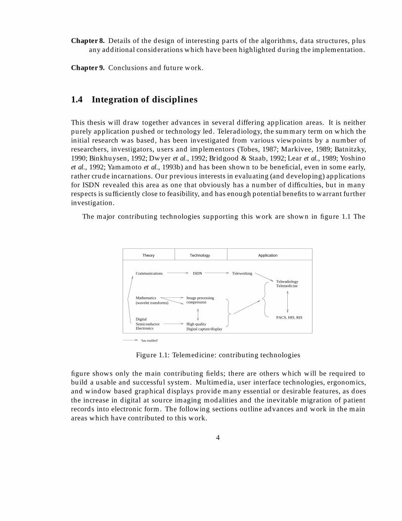
This thesis will draw together advances in several differing application areas. It is neitherpurely application pushed or technology led. Teleradiology, the summary term on which theinitial research was based, has been investigated from various viewpoints by a number ofresearchers, investigators, users and implementors (Tobes, 1987; Markivee, 1989; Batnitzky,1990; Binkhuysen, 1992; Dwyer et al., 1992; Bridgood & Staab, 1992; Lear et al., 1989; Yoshinoet al., 1992; Yamamoto et al., 1993b) and has been shown to be beneficial, even in some early,rather crude incarnations. Our previous interests in evaluating (and developing) applicationsfor ISDN revealed this area as one that obviously has a number of difficulties, but in manyrespects is sufficiently close to feasibility, and has enough potential benefits to warrant furtherinvestigation.

The major contributing technologies supporting this work are shown in figure 1.1 The

Mathematics Image processing

TechnologyTheory Application

Communications

(wavelet transforms)

ISDN

Teleradiology

PACS, HIS, RIS

Teleworking

Digital capture/displayHigh qualitySemiconductor

Electronics

Digital

‘has enabled’

compression

Telemedicine

Figure 1.1: Telemedicine: contributing technologies

figure shows only the main contributing fields; there are others which will be required tobuild a usable and successful system. Multimedia, user interface technologies, ergonomics,and window based graphical displays provide many essential or desirable features, as doesthe increase in digital at source imaging modalities and the inevitable migration of patientrecords into electronic form. The following sections outline advances and work in the mainareas which have contributed to this work.

4

1.5 Teleworking

Teleworking can be utilised in many situations where the worker is not required to be in anyspecific place to perform work, and requires only information and communication facilitiesto perform their job. Experiments in teleworking have been tried in many environmentsincluding telephony services, mail order, data entry, computing, bibliographic indexing, andpublishing, to name a few. Often the worker will operate from home with telephone, electronicmail, fax, and access to central computer facilities to provide the information necessary towork. There are many advantages of this style of working both for employers and employees.Employers can cut overheads, use remote or specialised labour, while employees can work athome with flexible or variable hours, and are not required to live within commuting distanceof an office. There are disadvantages as well of course, the major one of which seems to belack of interaction with other workers. However, some solutions are being tried, for instancevideophone usage for rest periods etc. Another recent idea is the ‘telecottage’ where a smallnumber of workers work from a building located close to the residential areas of villagesand towns, and which contains all the required computing, IT, and communication services.This solves the problem of workers being confined to home as they will meet others duringthe time at work, although all the workers might not be working for the same company andmight well be performing completely different jobs. Teleworking in general involves manyother issues which will not be considered here as we are interested in one specific application.

1.6 Medical imaging technology

Modern medical equipment makes extensive use of digital microprocessors with the resultthat much of the output is now readily available in digital form. For modalities where it is notthen analogue images are often digitised to enable on-line storage and processing. Soft copydisplay of images and information is becoming increasingly more common, and equipmentis being supplied with interfaces to allow connection to computer based networks and othermedical equipment.

Radiological Information Systems (RIS) and Hospital Information Systems (HIS) are termswhich usually imply textually based electronic information systems designed to performmainly administrative tasks, including scheduling, billing/accounting, resource allocation,staffing etc.

Picture Archival and Communication Systems or PACS usually refer to local (although notnecessarily) computer networks supporting image capture, archival and retrieval devices. Weexpect Teleradiology systems in the future to be linked to such networks, rather than beingdedicated point to point systems. In this scenario teleradiology is simply an applicationto be used over a LAN-LAN (local area network) or point to LAN interconnection. Wealso expect that future HIS, RIS, and PACS will use the same physical network, with theboundaries between each becoming blurred as information and functionality is necessarilyshared between them.

5

1.7 Telemedicine

Teleradiology has been considered as a telematic application for many years because ofthe very real benefits it can provide to medical practitioners and patients. It seems almostunfortunate that in terms of the quantity of information which is required to be transmitted,it is also one of the most demanding non video applications. The prospect of avoiding thenecessity for radiologists having to visit many different institutions, being available on-callduring out of hours periods, and having fast access to sub-speciality opinions has provokedmany to build trial systems.

More recently however, other medical activities are being considered for improvement byusing remote data access, consultation or teleworking. The details vary but many involve thetransmission of medical images as a key requirement.

1.8 Description of TR services

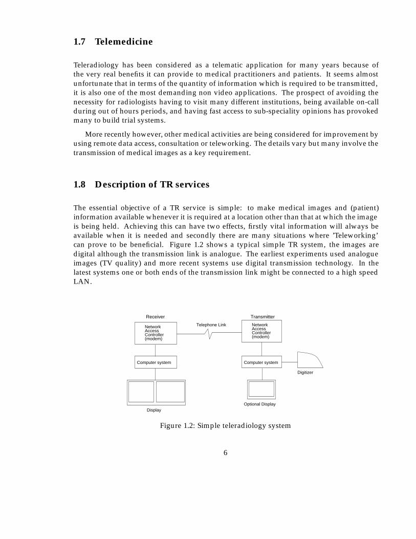
The essential objective of a TR service is simple: to make medical images and (patient)information available whenever it is required at a location other than that at which the imageis being held. Achieving this can have two effects, firstly vital information will always beavailable when it is needed and secondly there are many situations where ’Teleworking’can prove to be beneficial. Figure 1.2 shows a typical simple TR system, the images aredigital although the transmission link is analogue. The earliest experiments used analogueimages (TV quality) and more recent systems use digital transmission technology. In thelatest systems one or both ends of the transmission link might be connected to a high speedLAN.

Telephone Link

Transmitter

Digitizer

Receiver

NetworkAccessController(modem)

NetworkAccessController(modem)

Computer systemComputer system

Optional DisplayDisplay

Figure 1.2: Simple teleradiology system

6

1.8.1 Potential benefits of TR services

There are many potential benefits provided by having TR facilities available. In any specificimplementation local considerations such as geography, and health service provision policywill determine how effective a system will be in a particular situation. The following listsummarises some of the possible advantages:

� One radiologist can remotely serve several Cottage Hospitals, allowing an efficientservice with minimum delay.

� Consulting at a distance with subspeciality radiologists.

� Prompt interpretation of images at weekends or evenings.

� Radiologists in the community can gain immediate access to academic centres forproblematic cases.

� Forwarding of radiographic examinations to the primary referral centre prior to patientarrival.

� Availability of images from remote institutions.

� In cases of a fragmented radiology department, images can easily be made available toall radiologists.

� Possible availability of images direct from the scene of an emergency.

� Better information links can be made between hospitals and General Practitioners (GP).

� Wider availability of image data for training and medical research purposes.

� A reduction of professional isolation for practitioners in rural communities.

� Faster prior insurance approval of treatment (Farman et al., 1992).

These benefits will become increasingly important with the current trends in medical imagingfor instance those identified (Binkhuysen, 1992) in a paper reviewing the user interfaceproblems which must be addressed by system design. Namely:

� The use of non x-ray modalities such as ultrasound and MRI is increasing more andmore. An increasing number of referring physicians like to do their own imaging.

� Imaging modalities are becoming smaller and cheaper and the future is focused ondifferent groups of referring physicians. e.g. very small MRI’s for joints used byorthopaedic surgeons.

� The complexity of logistics (archiving, registration etc.) will be reduced when a fullscale PACS is integrated in the HIS/RIS.

Considering these trends we can perhaps envisage a greater need for remote more specialistconsultative services, supporting smaller community hospitals and physicians.

7

1.9 Image compression technology

The term ‘compression’ will occur frequently in this work and as it evokes much heateddebate when used in conjunction with medical imaging, the following paragraphs outline theview taken towards image compression throughout this work.

Compression can simply be defined as reducing the amount of data required to representsome original set of data. The reasons for doing this are usually straightforward; some setsof data can be very large, and hence expensive to use both in terms of storage and processingrequirements. An important implication of this for the TR application is the amount of timerequired to transmit an image through a communication channel.

It has been well publicised in recent years that most of the best 2 schemes lose or corruptsome of the original data. While this fact is undeniably true, the main objective is to ensurethat the information relevant to the purpose for which the image is to be used is not lost. Thereare problems with implementing this statement; we are often not able to make explicit therelationship between pixel data and diagnostic tasks. Many empirical studies have beencarried out which can give information like ‘resolution x is required in region y to enablepathologies of type z and minimum size q to be recognised’. In many applications it is fareasier to specify what is unwanted information rather that what is required, specifically it islikely that these type of criteria can be applied to each anatomical object. In many situationsthe subsequent use of an uncompressed image is defined well enough to allow the use ofrelatively simple criteria applied to quite sophisticated compression. In this way substantialsavings to be made in the medical image compression field without causing an effect on theoutcome of procedures carried out with those images.

Additional considerations often neglected include the loss of information when an imageis digitised from an analogue film, which is a generally accepted process due to the utilityof a digital image and also the possibility of processing and enhancing the digital version toreveal more detail than was visible on the original.

Finally experimentation has demonstrated that much of the ‘loss’ from an image is highfrequency noise, which is the most difficult component of the image to compress. Specifically,high quality images actually compress to a greater degree with less absolute pixel error. Oneresult of this can be a cleaning effect caused by performing the compression. We are notsuggesting this is always true, or even that it can be usefully employed, it does howeverprompt further investigation.

More detail on aspects of this discussion will be found in chapter 3.11.

1.10 Future applicability

During the course of this work we are aware that the use of fibre optical networks can providevast bandwidths of hundreds of Mbit/s or Gbit/s which effectively make the problem of

2taken to mean those providing large compression ratios, or large reductions in data volume

8

transmitting even the largest images in a fraction of a second trivial. Leaving aside argumentsof availability and economics which we might assume will eventually be solved, there remainseveral reasons for pursuing a low bandwidth solution:

� Any additional insight gained about the composition structure and characteristics ofthe application and images will be of use for other processes, for instance modelling,visualisation and analysis.

� Since the introduction of computing technology, resources (file space, network band-width) have only just kept pace with the requirements of application developers andusers. Indeed it will be many years before resources are inexpensive enough not to bea key issue in most PACS.

Although our teleradiology link might become faster, the image’s resolution and dy-namic range will increase as will the number of images, and the duration of theirstorage.

� Some of the methods developed are of a general nature and could be applied to otherapplication areas, for instance the progressive enhancement work would be useful forany pictorial interactive database browser.

1.11 What this work does not address

This work touches on some themes which have been the subject of philosophical, moraland political debates. Where appropriate these will be mentioned, but the issues will notbe pursued in detail as the technical aspects are our major concern. Though it is believedby the author that the ideas and techniques investigated in this work are sound, it wouldrequire further testing and evaluation, prior to implementation in a situation where significantdamage could be caused to persons by their use or misuse.

9

Chapter 2

Brief History and Review of RecentWork

As early as 1972 the prospect of using telephone circuits or radio frequency channels togive ‘images whose grey scale and resolution are satisfactory enough to be virtually indis-tinguishable from the original’ was being considered by some authors (Webber et al., 1973).The benefit of such a system was clear to Webber and his co-authors. Since this time anumber of experimental systems have been developed using various approaches based onthe technology of the time. Although many of these experiments have been small scale, andthe applications limited, they nevertheless have been important in providing informationconcerning technological, medical, psychophysical, and sociological implications in additionto providing an insight to the potential for telemedicine. It is important to consider the localinfrastructure, and practices when assessing how transmission of medical data might improveexisting systems of working. The examples in this chapter are taken from sources world-wideto demonstrate a number of (mainly technological) points, accordingly some would not beappropriate to all health care environments.

In the next section we review firstly a selection of experiments and the main conclusionsof these relevant to this work, secondly we review technology available today as a prelude toreconciling today’s technology with the facilities that are necessary, and those that can be seento be of potential benefit to medics and patients alike. Lastly we look to see where the currenttechnologies are likely to lead, as an attempt to assess any implications or shortcomings ofthe techniques being developed in this work to ensure its validity in the future.

2.1 Telemedicine: the early days

Initial telemedicine studies focused on teleradiology as a key application with only recentinterest in other potential teleservices. The early studies, of which two have already beenmentioned in the introduction, were based on analogue systems, with relatively low reso-lution. These experimental systems were built on ‘home made’ hardware as no commercial

10

offerings were available. It was initially thought that television quality would be adequatewhen provided with zoom facilities. Investigators soon discovered that the resolution wasinadequate for radiographic examinations and the signal to noise (S/N) ratio was too low withzoom facilities (Batnitzky, 1990). Transmission via UHF radio and line of sight microwavelinks was tried but proved to be difficult, especially in urban areas. Several trials using cabletelevision facilities (Curtis et al., 1983) underlined the resolution inadequacy of these systems.Although the success of experiments like these was low this was due to immature supportingtechnology and infrastructure.

2.1.1 Digital teleradiology

A major improvement was made with the introduction of digitised image data. Althoughthe digitised video image only provided a resolution of 512�512�81 the digital transmissionavailable via modems using the public telephone network proved to be adequate for someapplications. In 1982 the MITRE corporation under contract from the U.S. Public HealthService held a six month field trial involving four remote sites which transmitted radiologicalimages daily to a central clinic for reading by a radiologist. Leased telephone lines wereused to transmit 512�512�8 digitised radiological examinations. Evaluation via ReceiverOperating Characteristic (ROC) studies showed an accuracy of 96.7% for findings and 95.0%for impressions (Ratib et al., 1991a). Improvements in digitisation resolution allowed a secondtrial in 1985 using 1024�1024�8 digitised images, transmitted at 9600 baud over telephonelines. A similar evaluation to the 1982 study showed surprisingly, nearly identical results,although the subject matter of the images is not known.

The benefits of the use of TR in rural settings (Iowa, US) are highlighted in a sum-mary paper (Franken, 1992) which demonstrates ‘virtually identical’ diagnostic performancethrough the use of teleradiology, with significant (positive) effects on the family practitioner’slevel of confidence in diagnosis. The paper continues to outline three additional areas;Radiologist consultation to family practitioners in outlying areas, subspeciality consultationto radiologists in rural areas, and augmenting the availability of on site radiologists throughthe use of teleradiology.

The use of teleradiology for the emergency room is considered (Kagetsu & Ablow, 1992)using standard telephone lines and a modem, with a resolution of only 512�512 pixels. Aninteresting comment from the standpoint of this work was the following.

‘Limited spatial resolution makes the diagnosis of pneumothorax difficult ... Ifoptically zoomed images of both (lung) apices are routinely transmitted in additionto the PA and lateral view transmission time would increase ...’

The implication being that there is a specific region of these images which requires higherresolution than the rest. From comments such as these we developed the hypothesis that

1The convention n�m� bwill be used throughout to indicate an image of n pixels wide, bym pixels vertically,and b bit planes deep, giving 2b levels in a grey scale.

11

regional variations in the quality of images can be a useful feature, and also that it shouldbe possible to generate a high resolution image region from a lower quality one, withouttransmitting the entire pixel array. We return to these ideas in the following chapters.

2.1.2 Commercial offerings

The Kodak Ektascan Image transmission system provided a commercial offering in 1988 andwas also based on camera digitising of x-ray images displayed at 640�480�8 with zoomfacilities to enable an effective resolution of 1048�1920�8. It also provided an integral 9600baud modem for image transmission. An evaluation of the system (Markivee, 1989) (St. Louis(US) University Medical School) reported that diagnosis of digitised plain film radiographicimages was 98% accurate with the Ektascan unit, the study also indicated the importanceof image manipulation and simple image processing operations – including reverse video,window level adjustment and histogram equalisation – being used extensively to improvethe appearance of images.

2K2 TR technology was used in a study concerning cervical spine fracture detectionreported from the Arizona Health Sciences centre (US) (Yoshino et al., 1992). The studyused the DTR 2000 TR system, by DuPont (Washington). The resolution of this system was2048�2048�8, the images were transmitted via T1 (1.54Mbyte/S) leased land lines prior tobeing laser printed back on to film at the receiver for reading. The results which involved 4radiologists, showed no diagnostic difference for 2 of them between original and transmittedimages. The other two (the more experienced) did perform better with the original film. Theauthors provide the following interesting conclusion.

‘high resolution in and of itself is not adequate for fracture detection, and thatissues concerning image contrast manipulation also have to be addressed...’.

This advice has been accepted by many researchers, and a survey of modern systems revealsthat virtually all feature such image manipulation functions. It is our belief that such functions,with correct use, can more than compensate for degradation caused by digitisation, (andpossibly some forms of compression) of images. It is also clear that the resolution and qualityrequired for an image depends upon several factors, some abnormalities being less visiblethan others.

1993 saw encouraging results published in (Goldberg et al., 1993). A teleradiology linkwas set up using a 1.544Mbit/s T1 link, a 1684�2048�12 plain film digitise2, and an AppleIIfx interfaced to a 2048�2556 21 inch monitor as the diagnostic workstation. In addition a140 Gbyte optical jukebox was used for image storage, and a DEC VAX 6430 used as a fileserver. Each image was approximately 7Mbyte and took 36 seconds to transmit. Various otherspecialised hardware such as a parallel disk array for the file server and a custom displaycontroller for the diagnostic workstation were also required, with the following discussionincluded in this paper.

2FD-2000, Dupont, Wilmington, Del

12

‘Our results suggest that accurate primary diagnosis with high resolution digitalteleradiology is feasible. With an overall accuracy of 98% our results surpassedthe results reported with low and moderate resolution systems. Discrepancieswere judged by the review panel to be more closely associated with observerperformance than with any error introduced by the fidelity of the digital display’

The authors noted that 2048�2048 resolution monitors are likely to become standard in thefuture with 4096�4096 used for diagnosis of certain types of abnormalities. This could beprovided by zoom facilities based on the 2048 monitor. An additional mention is made to theeffect that the observers did not make much use of the magnification and intensity windowingfunctions. For soft copy displays to provide the best performance such features need to befully utilised and obviously be easy to use. Much of the work presented in later chaptersassumes that these facilities will be used to overcome the limitations of soft copy displays,given the many advantages.

At the time of writing the resolution of modern TR systems has stabilised at around 2K2

pixels for chest examinations (typically the largest) with debate about how much improvement4K2 systems would provide, if any. 2K2 has thus been used as the ‘typical’ resolution of largedigital x-ray in this work, to enable system and algorithm performance to be assessed.

2.1.3 Other modalities

The widespread use of images from other modalities has prompted investigations into thebenefits of using these in a TR environment. A number of additional factors are then broughtinto play, for instance some types of image are inherently digital, often at far lower resolution(256�256�8). This advantage is offset because some scans comprise of many images, or slicescreating a 3D image, thus making the transmission requirements extremely varied. Onesimple system (Yamamoto et al., 1993b) tested in 1991 (Hawaii) shows how simple technologyas a hand scanner, PC, and modem has been used to improve the ability of one medicalcentre to optimise patient transfers between outlying hospitals, based on transmission ofComputed Tomography (CT) scan information. In this case diagnostic quality images werenot considered necessary.

No difference in diagnosis was found during a study between 1988 and 1990 (Eljamel& Nixon, 1992) in the UK (Merseyside region) in which six peripheral CT scanners wereconnected to a centre for neurology and neuro surgery in Walton. Patients were transferredon the basis of images transmitted via an Image Link 100 system (Electronic imaging ltd,Oxford, UK). The main advantages of the system were in a reduction in unnecessary referrals,less complications during transport of critical patients due to unforeseen disorders, and earlydetection of some disorders by a precautionary local scanning policy. A detailed discussion ofthe economic advantages of the system is presented in the paper, but cost savings (excludingmedical, nursing, and police escort) were estimated to be around £20,000. Few technologicaldetails of the system are given but transmission time ranges from 2 - 15 minutes with anaverage of 5.5 minutes using standard (analogue) telephone circuits.

13

2.1.4 Other progress

The availability of switched digital dialup networks provide an additional flexibility, allowingoccasional usage patterns to be accommodated. In some locations it is possible to automati-cally select a number of channels. One TR study in 1991 (Kansas US) (Dwyer et al., 1992) allowsn�56Kbit/s channels to be selected, where n can be selected dependent on the time requiredfor transfer. The choice of bandwidth will depend exactly on the application, although anotherstudy (Honeyman, 1991) gives the unsurprising result that multiple 56Kbit/s lines are moreinexpensive than T1 5.44Mbit/s for low traffic situations between two specific destinations.

The promotion of ACR-NEMA DICOM (American College of Radiology/ National Elec-trical Manufacturers Association Digital Imaging COmmunications in Medicine) a standardformat for transfer of images and the all important associated patient information is verywelcome. The ACR-NEMA standard was originally designed to allow medical imagingequipment to be made plug compatible. The advances in LAN technology have madeinterconnection of equipment via industry standard interfaces, for instance Ethernet, andFDDI popular and many manufacturers are providing this type of connection to equipmentas standard. The ACR-NEMA DICOM standard has been improved to support the ISO(International Standards Organisation) communications model, and version 3.0 includesupper layer software support of TCP/IP. The DICOM standard has a vast array of predefinedfields for image and patient information, but necessarily is expandable through the use ofreserved codes. Therefore it would be possible to include the work of this thesis by the use ofthese links. We have not considered the details of implementing this step, however it wouldbe essential to provide an operational system.

2.2 PACS

Early investigations in teleradiology were based on stand-alone systems. This approach islimited to providing a remote diagnosis facility, and is only suitable in certain situations. Toprovide a more comprehensive service, allowing general access to information and imagesby a range of medical professionals, teleradiology should be considered part of a morecomprehensive PAC system. Only then will the major benefits of both systems becomeavailable. For the remainder of this work, we will generally consider that teleradiologysystems are likely to be part of some larger PAC system, with images which may or may notbe stored in some compressed formats.

Progress in implementing PACS has been slower than expected by many, with variousreasons being given. Aside from the financial considerations, the usability of the systemshas been seen to be a problem (Binkhuysen, 1992; Minato et al., 1992), with user complaintssummarised by:

� Systems are too slow.

� No good overview of an investigation or study is available.

14

� Comparison with previous examination images is difficult.

Retrospectively we discover that the techniques we have developed for teleradiology mightalso alleviate these problems in both remote and LAN based systems.

2.3 Leveraging technologies

Although many experiments have taken place in medical PACS and teleradiology in thepast, only recently have all the technological ingredients become available, with sufficientstandards (de facto or otherwise) to make an integrated digital medical imaging environmenta real prospect. Advances in technology have allowed these subsystems to be constructedby many medical institutions specialising in research. The storage and archive of medicalimages and data can be achieved with the use of high capacity optical disks and jukeboxes.Many consider that WORM drives have the advantage that images cannot become deleted orlost, while cost effective computed radiology equipment is becoming increasingly availableand portable digital x-ray equipment is also being developed. Many other image acquisitionmodalities are inherently digital and so are well suited to inclusion in PACS environments.Output devices allow high quality with reasonable cost. Laser printers can provide highresolution grey scale images and CRT monitors for soft copy have been arguably shown to becomparable to conventional film for diagnosis (H.Kangarloo, 1991; Goldberg et al., 1993). Thenetworking technology to link these devices into an integrated system has the form of highspeed optical fibre for PACS LANs, and possibly ISDN, or B-ISDN for the wide area network(WAN) aspects.

Much work has still to be done to make such systems readily and economically viable withthe advantages often not great enough to justify the massive investment. This is especiallyevident when some of the savings are not available directly, for instance the reduction ofarchive room space etc. Much of the required technology is still very expensive, and thesystems too fragile and complicated for the users, who are experts in their own fields, and donot wish to acquire vast amounts of computer expertise to be able to use new systems.

It is true however that the systems and trials performed more recently are far superior tothose only 5 or 10 years ago; the main factors contributing greatly to the improvement in TRand PACS systems in recent years are considered next.

Multimedia. The medical image workstation is essentially a multimedia environment, al-though it is often not explicitly called such. Typically an imaging workstation willallow viewing of images, text, and graphical figures. There is often a tape recordingdevice for reporting, and telephone access, and both of the latter could be integratedinto the workstation with minimal effort.

Communications. LAN technology is heading towards fibre optic media supporting manysimultaneous image (multimedia) transfers with real time performance to the user.

15

WAN technology can now support dial-up digital communications at medium band-widths and low cost. The bandwidth to the end user cannot increase much beyond thepresent levels until re-cabling with fibre or coaxial cable to each premises takes place.

Computing technology. High resolution display, and powerful workstations are becomingrelatively inexpensive, allowing WIMPS (Windows, Icons, Menus, Pointers) displaysand sophisticated image processing.

Archival devices. Optical jukebox technology (including RAID arrays) although still expen-sive allows large databases to be created and maintained, and has benefits of spacesaving and reliability compared with manual filing. As an additional benefit, there isno restriction to a single copy, unlike real films, which can be an advantage in someenvironments.

Imaging technology. Some commonly used modalities are inherently digital, often usingD/A conversion to produce video output. High quality digital scanners are nowavailable and films are often digitised when required.

Image compression. A leveraging technology bridging the gap between communications,and archive technology, and computing and imaging technology.

Standards. A number of useful standards are emerging; ACR-NEMA defines both hardwareinterfaces for equipment and also a structure for files in a PACS database. IEEE 802.3(Ethernet), FDDI, B-ISDN, and N-ISDN networking standards provide a variety ofbandwidths and possible services at various costs and availability.

Although these factors do allow PAC systems to be built, progress has been slow. The reasonsfor this are several; clearly changes in working practice combined with an (often justified)mistrust of technology are factors, exacerbated by few experienced commercial vendors alongwith incorrect expectations of what the new technology can provide. Additionally, heavyinvestment in hardware, software, and training is required.

2.3.1 Compression techniques

Compression algorithms are divided into two types, lossless and lossy. Lossless compressionalgorithms are bit-preserving and we thus recover exactly the same digital sequence as wascompressed. These techniques can be used for any type of information including text, images,graphics, sound etc. The best ones can achieve compression ratios of about 3:1 depending onthe type of data, with 2:1 or less being common for image data.

The other type of compression termed lossy does not preserve the data exactly, buttries to preserve all the relevant visual information. This can be very useful for images,for instance where the raw data is large and slight variations in the image bit pattern arevirtually invisible to the human eye, remembering that the initial digitisation already producessomewhat arbitrary (in terms of image content) spatial and intensity quantization. Lossy

16

image compression applied to medical images has been the subject of many discussions inthe past and it is true that lossy image compression should not be applied in an ad-hoc fashionto critical image data sets. However, if applied in sensible tested ways to images where theeffect on the image is known, and will not affect procedures to be carried out during the lifeof the image then the savings in storage and transmission time can be substantial, yielding10:1 - 40:1. Further discussion is postponed until section 3.11. Many experiments in applyingimage compression to medical images have been published (Bruce, 1987; Cetin, 1991; Choet al., 1991a; Aberle et al., 1993; Kajiwara, 1992; Sun & Goldberg, 1987; Popescu & Yan, 1993),and though results vary, they are on balance very encouraging. Details of the results of theseauthors findings are included in chapter 4 when we survey available techniques.

2.4 Diagnostic performance

The final objective of any medical imaging procedure is to make a correct and timely diagnosis.The extent to which this can be achieved depends on many factors, sometimes the limit ofdiagnostic performance is the imaging technique itself. This type of limitation is unavoidable,however it is important that any new techniques are at least as good and preferably better thanprevious ones. Unfortunately we are studying an area where performance is hard to predictas it involves skilled human operators who use experience and subjective processes whenreading an image and making a diagnosis. It is not always easy to predict the result of a specifictechnology, for instance the surprise result in section 2.1.1. For this reason many studies havebeen performed to decide what resolution and dynamic range is required for digital x-raysto produce similar results to analogue film. The usual technique is to employ a ROC study,which involves a number of radiologists diagnosing processed and original versions of a setof images, the statistical results of which can predict any performance differences.

After considering a number of studies (Aberle et al., 1993; Scott et al., 1993; Yoshino et al.,1992; Goldberg et al., 1993) it has become clear that for non digital modalities the process ofdigitisation can cause some reader errors, before any image compression has been performed.There are often multiple identified causes for this, not only lack of resolution or dynamic range.Studies aimed at finding minimum resolution requirements for a diagnostic task have foundretrospectively that many overlooked anomalies have been visible on the image, and thereforeother explanations have been sought. These include positioning of workstation monitorswhere there is glare on the screen, interruptions during the reading process, difficulty inusing the digital image enhancement facilities, or problems in comparing multiple images onscreen. The speed of image display can even cause a distraction from the diagnostic process.

Digitised studies which have printed images back on to film are immune to these problems,but do not have the on line image manipulation facilities available. Soft copy display hasboth technical and economic advantages over film which makes it likely to be the universalmedium for future imaging systems, therefore the problems associated with lack of userexperience or incapable user interfaces will diminish with time.

17

2.5 Future technology trends

Considering the technologies which contribute to PACS and TR systems a number of trendshave emerged. The imaging devices are producing higher quality images, and some modal-ities are becoming more compact allowing images to be produced on a more localised basis.The systems are becoming more usable with a better understanding of graphical user interface(GUI) construction and more powerful (and cheaper) processing to support these. Soft copydisplay is naturally accepted in some modalities where it is the primary viewing medium(e.g. NMI, Ultrasound) and is gradually gaining acceptance in other primarily film basedenvironments. Multimedia is becoming incorporated in a vast range of applications andmedical imaging is a naturally multimedium environment. Although archive technologyis based primarily around optical disks which can provide many hundreds of GBytes atfairly reasonable cost, storage of studies is still also sometimes a limiting factor. Fibre opticcommunication technology for LANs is feasible, as long as the system it supports providesenough added value to the institution, though it is still expensive. Wide area communicationis usually only feasible through the use of external carrier services, for some applicationsleased lines are appropriate, in the case of LAN-LAN interconnection for instance. However,these are expensive if utilisation is low, the alternative of using switched dialup services isoften the best solution for ad-hoc or low volume connections. For the best coverage ISDN at64 or 128 Kbit/S is widely available and can connect to most places including the GP surgery,remote clinics, and (on call) radiologists homes, at very low cost.

It is hoped that the work of this thesis might help in two ways, firstly to allow the provisionof extra value added (tele) services, and secondly to allow savings on bandwidth/ storagerequirements which would improve feasibility by lowering the cost of existing imagingservices.

18

Chapter 3

Facilities Required to ImplementImage Based Telemedicine

This chapter is primarily concerned with ascertaining the users’ requirements for medicalteleimaging1 and then linking these to the characteristics which will support this within thetransmission and image compression technology. Some sections of this chapter are extractedfrom a previous publication by the author (Snooke, 1992).

3.1 Requirements of the professional user

A number of general requirements have been identified from the literature which a TR systemmust meet to be considered usable:

� It should not interfere with diagnostic procedure.

– No noticeable or distracting delays.

– Appropriate resolution and grey scale.

– Flexible and powerful (graphical) user interface.

� Diagnostic facilities should at least match those already available.

� The system should require minimum familiarisation time for a new user, but should notbe frustrating for the expert user.

The way in which these objectives will be met depends partially upon the type of servicebeing provided. We can identify two different situations:

1the term teleimaging has been adopted to encompass a greater range of imaging modalities applications thanteleradiology

19

� Advance notice of the transmission of an image or study is available — either explicitly,or from an intelligent HIS or PACS system by workload scheduling.

� Immediate transmission is required —‘wet reading’ for consultation, second opinion,emergency use, and teaching/reference.

Consideration of the published trials and studies would indicate that the transmission of manyimages can be determined in advance, for instance most routine interpretation performed byradiologists can be scheduled hours or possibly days in advance. When we consider possibleaccess to images by others, for instance by GPs, it is likely that these do not often require fullprimary diagnosis quality images.

3.2 Types of user

Although primary diagnosis of radiographs by a radiologist is the main scenario in theteleradiology literature and for this research, there are a number of situations where remoteaccess to medical images is (potentially) useful.

Teleradiology. Useful for small institutions, subspecialty situations, contract radiology etc.

Second opinion. Typically when a radiologist, doctor, or consultant would like a secondopinion, a delay is initiated while the image is transferred by post, or a visit is made.Particularly in small institutions where the range of expertise is limited this can be asignificant problem. The advantages of electronic transfer of diagnostic quality imagesor real time multimedia consultation are obvious.

Outpatient clinics. Though not essential, images can in some circumstances be of benefitduring tertiary care. Diagnostic quality is not necessarily required, for instance 8 bitdisplay rather than 12 bit, with limited image manipulation ability (London & Morton,1992).

Doctor’s surgery. The GP typically does not have access to images currently, however exper-iments in making such information available are being considered. Again only ‘reviewquality’ is desired.

Remote retrieval. Over a period of time one specific patient might have images archived ina number of places. Inter hospital image communication can sometimes reduce thenumber of additional images which need to be made.

Training/ education/ reference. Images which are used for education, or those that showsome particularly interesting item should be available (anonymously) to the radiologicalcommunity. Due to the limitless copies available electronically reference images can bemade available for the cost of transmission.

Archive. In some situations remote long term archival is economically more viable whenperformed in bulk at regional centres.

20

3.3 Primary functions of a medical imaging network

A PACS or TR facility can be considered as 4 major subsystems:

� Image acquisition.

� Database and storage.

� Display and output.

� Communication network.

For a typical PACS system the TR link will be between the database and remote displaysystems although there are circumstances where other combinations of subsystems might belinked remotely.

In the case of a regional archive facility the small scale hospital PACS database could bearchived periodically to a remote long term storage facility.

The Acquisition and Display/Storage systems might also be linked remotely. For instancein situations when portable imaging equipment is available at the scene of an emergency, theimage can be available at the hospital prior to patient arrival. Potentially, advice could evenbe given to personnel at the scene of an emergency.

3.4 Teleradiology network requirements

The following criteria have been proposed as desirable requirements of a wide area networkor a TR system (Honeyman, 1991). Indeed, we note that when they are satisfied it will bepossible to provide a service which will satisfy the user requirements given in 3.1.

� Image data is accepted rapidly by the WAN.

� The WAN promptly accepts an intended transmission.

� The WAN is efficient (no long idle periods).

� Image data arriving at receiving host computer is processed rapidly.

� Transmission protocol responses are processed rapidly.

� The topological connectivity is modifiable in a reasonable length of time.

� The WAN is transparent to the user.

� The WAN should be as cost effective as possible.

21

To satisfy all these requirements is very difficult, in particular the technology required isexpensive - possibly too much so to fulfil the cost criterion. In the future B-ISDN might wellprovide a complete solution, however, at the present time it is still not widely available, andis expensive especially in the rural areas which have been identified as benefiting most fromthe TR services.

If we consider the circuit switched 64K bit/s ISDN network it satisfies most of the criteriato the following extent.

Prompt acceptance. Once a call has been placed the sender has exclusive use of the channeland so there should be no delay prior to sending data. If a call is not active a call set updelay of the order of a few seconds should be acceptable in most cases.

Efficient use of WAN. Calls can be dropped according to a suitable strategy once active useof the line has ceased. There are a number of factors to take in to account when decidingon such a strategy, particularly in relation to the carrier’s tariff arrangements.

Connectivity. This is one of the strongest features of the ISDN. It should be possible toconnect to any required location (given access authority restrictions) that have therequired server machines.

Transparency. The public service telephone network (PSTN) already provides this, as willISDN calls. Systems will obviously be required to be configured to connect to the correctdatabases, but this is likely to be under ‘friendly’ user control.

Host computer responses. The host machine should not cause delays to the system, eitherin accepting data, or processing responses. We do not see this as a problem, given thatreasonably powerful and inexpensive machines are available, and are required in anycase for other aspects of this type of application.

Cost. The cost will depend on configuration, and usage patterns in any specific implementa-tion. A cost effective solution is anticipated if the other criteria can be met.

Throughput. Although N-ISDN has far greater throughput than was previously possibleusing modems and the like, large high quality images contain massive amounts of rawdata, making this the main unresolved problem area to which we turned our attention.

3.5 Application to rural areas

Rural areas have many difficulties on top of those experienced by well populated urban areas.Some of the more obvious are as follows:

� Part time staff — some radiologists serve several hospitals visiting each on one or twodays each week. This causes delay to some patients, and the radiologist’s time is notproductive whilst travelling.

22

� Few local specialists — it is not feasible or economic to employ many specialist consul-tants in smaller hospitals. Patients therefore find it can take days or weeks for diagnosisto be made, the method used to send images often being by land mail.

� Central storage of electronic images — it might prove more effective to collect imagesin a central database where the necessary hardware and staff can be employed ratherthan burden cottage hospitals with this expense.

� When it is necessary to refer a patient to another hospital the relevant images can bemade available prior to his/her arrival and if necessary an interactive session betweenthe staff concerned could be arranged utilising image, voice, and graphic media.

3.5.1 Workstation requirements

Within a PACS or TR environment several types of workstations are required to satisfythe various requirements of the users. In one study (Matthews, 1991) 5 differing types ofworkstation were proposed:

Specialised image stations. An interface between acquisition unit and medical and technicalusers.

Image Processing Stations. Powerful machines with multiple level user interface to enableuse by engineers, specialists, clinicians, programmers etc.

Multimodality Reporting Console (MRC). Interpreting and reporting of exams. Two typesmultiple display (several monitors) and virtual display (roam, pan, zoom on single moni-tor).

Multimodality Viewing Station (MVS). For review by clinicians, user friendly but not so-phisticated.

Remote Viewing Stations (RVS). To review images at remote sites and scientific archive(s).

The details of the functionality for these can be found in (Matthews, 1991). Althoughthe RVS here is assumed to have a low functionality to enable remote access, it would bepossible for any of the other types of workstation to utilise remote images given a reasonablyrefined communication system. MRC’s would be necessary for a remote interpretationservice, with MVS and RVS being reduced functionality versions with possible applicationto GP and archive site access. A paper dealing with how to evaluate a medical imagingworkstation (Johnson et al., 1987) although now dated, demonstrates the requirement forvarious workstation capabilities. The evaluation is based within a framework for categoriesof task (verification, interpretation, and consultation) and types of user (technician, physician,hospital or clinic). Acceptable parameters (e.g. resolution) depend upon the location withinthe framework. Other authors have considered less specific categories than these, and a moregeneral approach such as the use of X-terminals provides a sufficiently flexible approach

23

(London & Morton, 1992) to enable diverse information including text, images, and graphsto be included. In the situation where significant local processing is required the server andclient can be supported on the same (powerful) local machine. In other situations, especiallywhen connected via fast LANs to powerful processors, then an X-terminal server would besufficient, utilising remote clients.

It is clear that although different capabilities are required for the different tasks, a modularapproach comprising both hardware and applications gives greater flexibility plus economyof scale.

3.5.1.1 ACR-NEMA

The need for a standard way of interchanging images from different manufacturers’ ma-chinery was realised over a decade ago. This prompted ACR-NEMA to develop the DigitalImaging and Communication (DICOM) standard. The PAPYRUS format based on ACR-NEMA DICOM with additions by the TELEMED project working group appears to be aflexible solution (Ratib et al., 1991b). A folder mechanism is used to prevent images frombecoming separated from related patient details and clinical information. In addition, a framework for storing the large numbers of parameters associated with most medical images isprovided based on a ‘tagged’ format. Some simple types of image compression are supporteddirectly, however spare locally defined user fields can be used to support ‘non standard’techniques.

3.5.2 End user terminal expectations

From a survey of the literature (Okabe et al., 1991; Ratib et al., 1991b; Johnson et al., 1987;London & Morton, 1992; H.Kangarloo, 1991) the following list of expected features for primarydiagnostic level workstations has been compiled. The extent to which each is necessary cannotbe ascertained without specific application requirements. The following list is includedprimarily to ensure that operational aspects are not overlooked in future chapters.

� High quality graphics display — 10242 or 20482 pixels.

� Powerful graphical user interface.

� Local disk storage — sufficient for storage of advance studies and temporary processedimages.

� Frame store or fast RAM — to provide fast switching between images in a study,especially if a single monitor system is being used.

� Image compression software or hardware.

� Image manipulation processing capabilities — there are many essential image process-ing operations to aid diagnosis. These are discussed in 3.5.3.

24

� Possible multimedia support.

� Suitable network connection and supporting protocols. This could include voicecommunication facilities with an ISDN workstation.

� Transparency of network — the radiologist should not need to know about the topologyof the network to access the required images. Items such as patient name, ID, andhospital should be adequate to locate images. We shall not dwell on this here as forlarge distributed databases this is a complex problem studied by others.

� Security — Access to confidential information must be restricted to authorised person-nel. A multi level access system would perhaps be required.

Multimedia technology appears to have many advantages for the medical workstation. Itis possible that verbal as well as textual reports could be made, consultation between remotespecialists will be enhanced by animated graphical overlays on images. Most specificationsfor medical imaging workstations already implicitly combine aspects of multimedia, otherfunctions will be included as natural progressions as the technology matures.

3.5.3 Image manipulation / processing functions

Although the field of medical imaging uses many very specialist image processing techniques2

there are a number of facilities that have been found to be particularly useful and are applicableto many types of image. These fall into 3 categories; manipulation, processing, and annotation:

Manipulation The content of the image data is not changed, only the users’ view of it.

Processing The content of an image can be modified.

Annotation Appending additional information to an image ( textual, pictorial, audio etc ?).

The following list is a compilation of techniques (Irie, 1991; Okabe, 1991; Ligier et al., 1992)which we have divided in to the above categories.

Manipulation functions:

� Intensity level modification (brightness).

� Intensity level remapping (windowing).

� Magnification and interpolation.

� Minification3, Spatial Information Models.

2for instance in 3 dimensional reconstruction3Display of several reduced size images on a single monitor, similar to a pictorial directory or catalogue of

image files

25

� 3-D display.

� Dynamic display.

Processing functions:

� Histogram equalisation (contrast enhancement, global and local).

� Edge enhancement.

� Weighted addition or subtraction of images.

� Frequency enhancement.

Annotation functions:

� Measurements of distance and angle.

� Editing or annotation of images.

� Region of interest (ROI) identification.

Most of these functions are easy to achieve with any workstation of reasonable power, certainlythe manipulation functions will be required to enable a graphical user interface to performefficiently.

3.5.4 User interfaces

An important area neglected until relatively recently can make or break a system. If theuser interface is poorly designed, it makes no difference how good (or fast) the rest of thesystem is - it won’t be accepted by the users ! Windowing environments like X Windows forworkstations or Microsoft Windows for PC’s can provide a relatively consistent and intuitiveinterface to sophisticated software. These environments are ideal where multiple images areto be manipulated and displayed, and can (for X-windows) allow multiple screens to be usedfor applications if necessary.

3.5.5 Bandwidth availability

Restricting the long distance communication to basic rate ISDN requires that we use 64K bpsor multiples thereof. In many situations it would be possible to utilise both the B1 and B2channels with the option of adding more channels bandwidth. For the following sectionshowever, we restrict bandwidth to 64 or 128Kbps switched lines, ignoring the possibility ofpacket or frame relay based services with higher transient throughput.

26

3.6 Modes of working

It is useful to define categories of modes of working and determine the constraints eachhas with regard to the network performance measures such as average throughput, peakbandwidth, latency etc.

The categories are based on considering a communication link which has at each end eithera medical professional (P) or the database containing the images (D). In all cases assumingthat every local network connecting devices at either end is faster than the wide area linkunder consideration, and provides sufficient buffering so that delays and transmission timesbetween a local review console and database are small.

session

Reactive

P -- D P -- PD D -- D

-- link P user D database

Tele medical reporting

advance

Emergency or

Tele medical reportingfresh studies

Database archieve

interaction

session type

Review sessionsConsultation

Consultation

multiple patient/studyStructured

On the fly consultation

requestspurious additional

52

3

1 4

6

7Scheduled

Figure 3.1: Modes of working

Referring to figure 3.1 we can identify several situations based on the above categories:

1. A number of studies are to be diagnosed and reports returned. The process (for x-ray interpretations) in some countries is known as contract radiology, and can beperformed remotely as no patient interaction is necessary. Often the images couldbe transferred before the radiologist starts work, provided sufficient storage is availableon the workstation.

2. Another situation can exist where the radiologist will indicate which studies are goingto be required as each session begins.

3. All other situations can be considered as ‘wet reading’4 the most demanding situation,when an image is required for viewing instantly.

4wet reading as used by (Bridgood & Staab, 1992) to indicate the situation when the radiologist is waiting forthe image to be transmitted

27

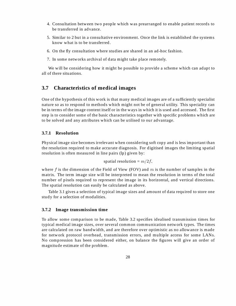
4. Consultation between two people which was prearranged to enable patient records tobe transferred in advance.

5. Similar to 2 but in a consultative environment. Once the link is established the systemsknow what is to be transferred.

6. On the fly consultation where studies are shared in an ad-hoc fashion.

7. In some networks archival of data might take place remotely.

We will be considering how it might be possible to provide a scheme which can adapt toall of there situations.

3.7 Characteristics of medical images

One of the hypothesis of this work is that many medical images are of a sufficiently specialistnature so as to respond to methods which might not be of general utility. This speciality canbe in terms of the image content itself or in the ways in which it is used and accessed. The firststep is to consider some of the basic characteristics together with specific problems which areto be solved and any attributes which can be utilised to our advantage.

3.7.1 Resolution

Physical image size becomes irrelevant when considering soft copy and is less important thanthe resolution required to make accurate diagnosis. For digitised images the limiting spatialresolution is often measured in line pairs (lp) given by:

spatial resolution = m=2f;

where f is the dimension of the Field of View (FOV) and m is the number of samples in thematrix. The term image size will be interpreted to mean the resolution in terms of the totalnumber of pixels required to represent the image in its horizontal, and vertical directions.The spatial resolution can easily be calculated as above.

Table 3.1 gives a selection of typical image sizes and amount of data required to store onestudy for a selection of modalities.

3.7.2 Image transmission time

To allow some comparison to be made, Table 3.2 specifies idealised transmission times fortypical medical image sizes, over several common communication network types. The timesare calculated on raw bandwidth, and are therefore over optimistic as no allowance is madefor network protocol overhead, transmission errors, and multiple access for some LANs.No compression has been considered either, on balance the figures will give an order ofmagnitude estimate of the problem.

28

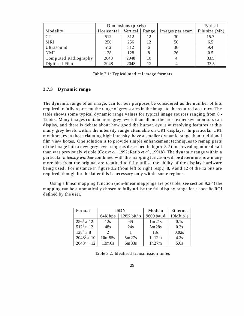
Dimensions (pixels) TypicalModality Horizontal Vertical Range Images per exam File size (Mb)CT 512 512 12 30 15.7MRI 256 256 12 50 6.5Ultrasound 512 512 6 36 9.4NMI 128 128 8 26 0.5Computed Radiography 2048 2048 10 4 33.5Digitised Film 2048 2048 12 4 33.5

Table 3.1: Typical medical image formats

3.7.3 Dynamic range

The dynamic range of an image, can for our purposes be considered as the number of bitsrequired to fully represent the range of grey scales in the image to the required accuracy. Thetable shows some typical dynamic range values for typical image sources ranging from 8 -12 bits. Many images contain more grey levels than all but the most expensive monitors candisplay, and there is debate about how good the human eye is at resolving features at thismany grey levels within the intensity range attainable on CRT displays. In particular CRTmonitors, even those claiming high intensity, have a smaller dynamic range than traditionalfilm view boxes. One solution is to provide simple enhancement techniques to remap partsof the image into a new grey level range as described in figure 3.2 thus revealing more detailthan was previously visible (Cox et al., 1992; Ratib et al., 1991b). The dynamic range within aparticular intensity window combined with the mapping function will be determine how manymore bits from the original are required to fully utilise the ability of the display hardwarebeing used. For instance in figure 3.2 (from left to right resp.) 8, 9 and 12 of the 12 bits arerequired, though for the latter this is necessary only within some regions.

Using a linear mapping function (non-linear mappings are possible, see section 9.2.4) themapping can be automatically chosen to fully utilise the full display range for a specific ROIdefined by the user.

Format ISDN Modem Ethernet64K bps 128K bit/s 9600 baud 10Mbit/s

2562� 12 12s 6S 1m21s 0.1s5122� 12 48s 24s 5m28s 0.3s1282� 8 2 1 13s 0.02s20482� 10 10m55s 5m27s 1h12m 4.2s20482� 12 13m6s 6m33s 1h27m 5.0s

Table 3.2: Idealised transmission times

29

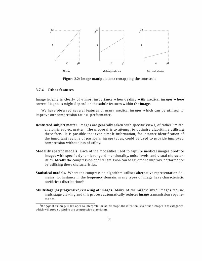
28

122

c’

c

28

122

c’

c

28

122

c’

c

Normal Mid range window Maximal window

Figure 3.2: Image manipulation: remapping the tone scale

3.7.4 Other features

Image fidelity is clearly of utmost importance when dealing with medical images wherecorrect diagnosis might depend on the subtle features within the image.

We have observed several features of many medical images which can be utilised toimprove our compression ratios/ performance.

Restricted subject matter. Images are generally taken with specific views, of rather limitedanatomic subject matter. The proposal is to attempt to optimise algorithms utilisingthese facts. It is possible that even simple information, for instance identification ofthe important regions of particular image types, could be used to provide improvedcompression without loss of utility.

Modality specific models. Each of the modalities used to capture medical images produceimages with specific dynamic range, dimensionality, noise levels, and visual character-istics. Ideally the compression and transmission can be tailored to improve performanceby utilising these characteristics.

Statistical models. Where the compression algorithm utilises alternative representation do-mains, for instance in the frequency domain, many types of image have characteristiccoefficient distributions5

Multistage (or progressive) viewing of images. Many of the largest sized images requiremultistage viewing and this process automatically reduces image transmission require-ments.

5the type of an image is left open to interpretation at this stage, the intention is to divide images in to categorieswhich will prove useful to the compression algorithms.

30

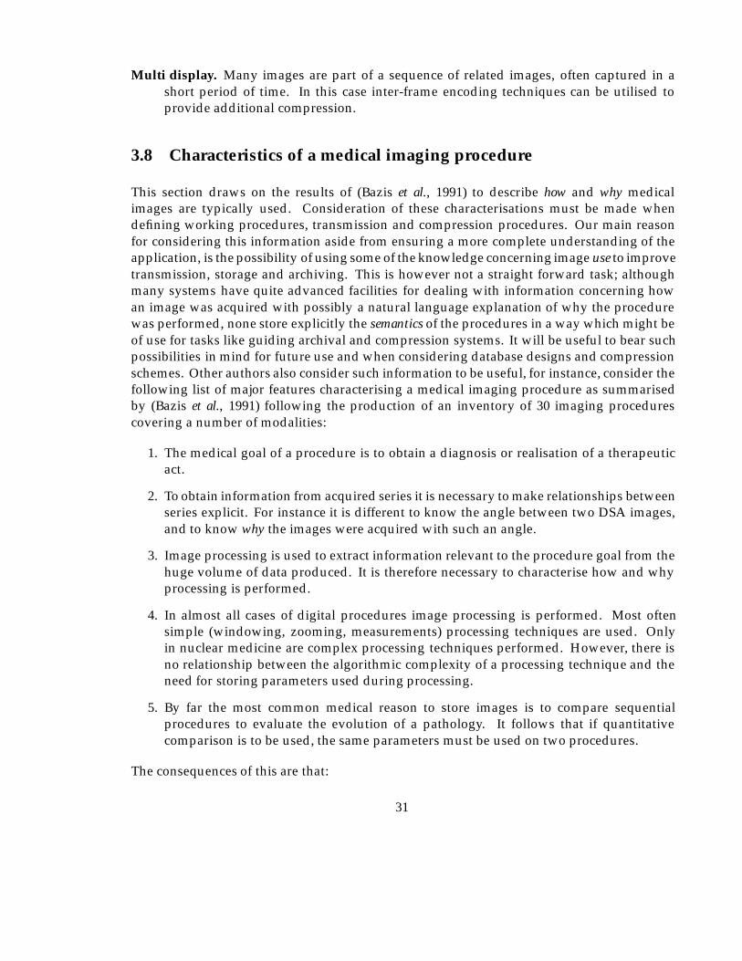
Multi display. Many images are part of a sequence of related images, often captured in ashort period of time. In this case inter-frame encoding techniques can be utilised toprovide additional compression.

3.8 Characteristics of a medical imaging procedure

This section draws on the results of (Bazis et al., 1991) to describe how and why medicalimages are typically used. Consideration of these characterisations must be made whendefining working procedures, transmission and compression procedures. Our main reasonfor considering this information aside from ensuring a more complete understanding of theapplication, is the possibility of using some of the knowledge concerning image use to improvetransmission, storage and archiving. This is however not a straight forward task; althoughmany systems have quite advanced facilities for dealing with information concerning howan image was acquired with possibly a natural language explanation of why the procedurewas performed, none store explicitly the semantics of the procedures in a way which might beof use for tasks like guiding archival and compression systems. It will be useful to bear suchpossibilities in mind for future use and when considering database designs and compressionschemes. Other authors also consider such information to be useful, for instance, consider thefollowing list of major features characterising a medical imaging procedure as summarisedby (Bazis et al., 1991) following the production of an inventory of 30 imaging procedurescovering a number of modalities:

1. The medical goal of a procedure is to obtain a diagnosis or realisation of a therapeuticact.

2. To obtain information from acquired series it is necessary to make relationships betweenseries explicit. For instance it is different to know the angle between two DSA images,and to know why the images were acquired with such an angle.

3. Image processing is used to extract information relevant to the procedure goal from thehuge volume of data produced. It is therefore necessary to characterise how and whyprocessing is performed.

4. In almost all cases of digital procedures image processing is performed. Most oftensimple (windowing, zooming, measurements) processing techniques are used. Onlyin nuclear medicine are complex processing techniques performed. However, there isno relationship between the algorithmic complexity of a processing technique and theneed for storing parameters used during processing.

5. By far the most common medical reason to store images is to compare sequentialprocedures to evaluate the evolution of a pathology. It follows that if quantitativecomparison is to be used, the same parameters must be used on two procedures.

The consequences of this are that:

31

“To be medically useful a Medical Image Data Base (MIDB) must be able to storeevery piece of information used during the realisation of a procedure, and duringits consumption. If this is not the case the medical interest of a PACS is significantlydecreased.”

The paper concludes that a minimal MIDB solution is possible with standards like ACR-NEMA, however for a generalised solution which stores the semantics of each procedure, afar more complex data base is required;

“...since image sources, archives and workstations are not fully disconnected:archives must know how acquisition and processing are done in image sourcesand workstations to make it clear to final users why it was done (in terms of amedical goal).”

Although this was written in the context of providing a value added system that physicianswould gain benefit from using, we had previously considered the use of such informationto improve the efficiency of compression algorithms, or more specifically to enable lossycompression to be used in a more useful way. It is now clear that a PACS or MIDB shouldbe more than purely an image extension to current HIS systems. Achieving this though isnot an easy task, particularly given the many possibilities that WAN technology provides forremote teleservices.

3.9 Techniques for image transmission

It is clear that many of the circumstances in which images must be transmitted, are amenableto N-ISDN bandwidths. The following sections investigate methods which we considerutilising to provide a service for the wet reading situations.

3.9.1 Predictive transfer

Predictive transfer or intelligent scheduling covers a wide variety of situations where infor-mation obtained by the PACS and HIS system can predict which images will be required at aremote location. This can range in the simplest form from checking a radiologists’ workloadschedule, to locating and transmitting a relevant archive image for a patient, or perhapsautomatically selecting the correct portion of an image for progressive enhancement basedon the information in the image request given to the radiographer or technologist when theimage was requested, for instance, what the main region of anatomy to be considered is.

If we consider the simplest case of a scheduled viewing of a set of studies we can considerthe feasibility of transmitting the images during a viewing session. Using S to representthe average study size (bytes), t as the average time (sec) taken to view an image (perform

32

diagnosis, write report etc.), and b as the bandwidth of the communication to the remotedatabase, if we assume full utilisation of the bandwidth and buffering then

S

t� b:

If we insert t = 300s (Willis, 1991), and b = 64K bit/s then we obtain 2.4M bytes per study asan approximate sustainable throughput. To determine required compression ratio we mustobtain the type and number of images per study for each application. Using this scheme thedelay prior to displaying each image should be small, with the exception of the first requestfor each session for which it will be necessary to wait.

In practice the image sizes and viewing times are variable thus requiring enough bufferingto accommodate storage of images to allow the bandwidth of the line to be fully utilised. Somedelays might occur near the beginning of a session if especially rapid use of images is made.

3.9.2 Image compression

“Image compression algorithms have a key role to play as a leveraging technology in imagemanagement systems” (Cho et al., 1987). There are many image compression methodsavailable and they fall into two categories; lossy, and bit-preserving. Generally bit-preservingmethods can only provide 30% to 60% compression of the original image, however they areconsidered ‘safe’ as the original pixel values in the image can be recovered exactly from thecoded one. The lossy methods can compress to 5% or less of the original image size, howeverit is possible that some detail might be lost from the image. It is therefore necessary to exercisegreat care to ensure that relevant information is not lost.

When choosing lossy compression an image can be compressed to a given size (orequivalently, ratio) or a given quality measure can be chosen. The latter measure provides thesafest technique allowing complex hard-to-compress images to attain a lower compressionratio than ‘simple’ images. When designing encoding schemes, quality should always be theprimary constraint, with compression ratio secondly. This can have significant effects on thealgorithms which are developed. For instance, we should select the number of coefficientsrequired to attain a given quality, rather than selecting a given number of coefficients to attaina specific ratio. Refer to chapter 7 for more details on quality measures and chapter 4 for areview of compression technology.

3.9.3 User acceptance problems

Because interpretation and diagnosis is a subjective practice learned through experience it isdifficult to predict what effect any particular change in working practices or equipment willhave on the overall performance of the human expert concerned. For this reason it is oftenadvantageous to imitate established practices and equipment using the new technology, forinstance multiple monitors to simulate the traditional ’light box’ illuminator used in viewing

33

films. Problems of ‘user adjustment’ are often encountered in studies involving a slight changein working practice. An example is digital image manipulation – a powerful tool which canovercome the limitations of soft copy display – however even when the implementation isgood, the users often do not make use of the facilities available without specific coaxing.Once the practice of using the new facilities is established the problems have been overcome.Our conclusion is that user reservation should be taken seriously (often concerns are fullyjustified) but should not unnecessarily retard the investigation of new techniques.

3.10 Time criticality

It is now clear that ISDN has the potential to provide acceptable communication of images insome circumstances. To attempt to find solutions for the demanding interactive transmissionof images additional techniques need to be considered.

3.10.1 Progressive enhancement

Progressive enhancement is useful for interactive transmission. The image is built up instages starting with a low quality ’sketch’ and rapidly improving to include fine details.The advantage is that the user might be able to select the important region quickly, thuseliminating much of the transmission, as only this area needs to be sent. The idea of usingprogressive enhancement for the transmission of medical images is not new, many of thearguments for its use are discussed elsewhere (Elnahas et al., 1986) in conjunction with adiscrete cosine transform (DCT) based implementation. In some cases the region of interestmight be identified automatically from the image by the use of image processing techniques.For instance, the background of an image is unlikely to be of interest. The section of theimage most relevant to the study will then become visible first, with the rest of the fine detailappearing subsequently, should it be required. Decompositions in the frequency domain areideal for this as the low frequency parameters can be transmitted initially followed by thehigh frequency parts subsequently, thus omitting the fine detail initially so producing theeffect of a ‘blurred’ , but recognisable image useful for navigation and selection.

Progressive enhancement systems do not necessarily involve any feedback from thereceiver. Many have a pre-determined sequence of quality enhancing iterations, with theonly user interaction being premature termination of the transmission. We consider it wouldbe far more useful if the receiver can provide feedback to guide the transmission to matchuser requirements. We envisage three categories of receiver feedback:

Terminal, hardware, or configuration settings of remote access terminals can supply infor-mation which can affect the image reproduction strategy.

By-products of user actions can be utilised to imply certain information about what charac-teristics of the image are required.

34

Direct user requests The user should be free at any time to request additional improvementson any aspect of the image.

The following table gives a number of progressive enhancement requests for each of thecategories, and typical ways in which the system might respond.

Category Nature EffectTerminal, or configuration settings

display size quick display on lower resolution systemquick display on split/ windowed screen(s)

pixel depth (planes) efficient 12 bit image on 8 bit displaydiagnostic or review quality optimum selection (eg. GP Info)communication network efficient update stepsother heuristics e.g. prioritise centre portion at better quality

By-products of user actionszoom capability higher resolution

or spatial frequency componentsintensity windowing more accurate approximation for LF components

more bits/ planesmulti image display reduced effective resolution and less HF required

Direct user requestspriority regions regional quality improvementSIM selection expand updateSIM region selection expand, prioritise regionbest possible receive allopen folder transmit textual reports plus SIMS

3.10.2 Region of interest identification

Many medical images are of well defined types with specific features and interest areas. Withimage segmentation and modelling techniques, identification of large areas of low interestwithin an image will allow savings in transmission and storage capacity. We divide the ROIidentification into two categories, user identified and automatically identified.

The user identified ROI approach is used during reading or processing of an image byradiologists or technologists. The technique is commonly used during soft copy processingto identify sections of an image for further manipulation or processing as mentioned earlier.The simplest method most often encountered in the literature is the ‘click and drag’ operationusing a mouse or similar device to produce rectangular ROIs. We have considered thatthe ROI might be used to select the important areas of an image when it is being accessedremotely over lower bandwidth channels, allowing the quality to improve from good toexcellent (or original) quality rapidly within the selected region. The transmission of large

35

volumes of data can thus be avoided. There are obvious limitations to this approach asit will involve additional user interactions, and possibly small delays. However, assumingdiagnostic accuracy is not affected by these user interactions, there are circumstances in whichthere will be overall gains.

Automatic identification is where we see much future development. It will be possible forregions of each image to be identified, and manipulated to provide the radiologist with thebest possible view of the image - without (or with minimal) user assistance. Some automaticprocedures are already carried out on digital radiographs to enable good visual display dueto the extremely good linear dynamic range of the images. We note that out of three methodsconsidered for performing this intensity rescaling (Blume & Kamiya, 1987), the techniquewhich has actually been used medically requires a model in terms of the characteristichistogram features, for each type of image, to calculate the capture and display scalingand auto-ranging parameters. The method put forward as possibly being the best (futuremethod) requires specific anatomical features to be automatically identified to allow auto-ranging based on anatomy as well as imaging technique and various diagnostic specifiers.This is in essence similar to automatic ROI enhancement, and as such it should be possibleto extend the methods to allow images to be highly compressed without danger of losingimportant diagnostic information. We note that as the compression algorithm would beobliged to preserve information in poorly recognised/defined areas the compression ratiowould be governed to some extent by the quality of the identification of regions.

Unfortunately no details were given of how the various anatomical features wouldbe identified, though this technology is certainly not new, as researchers have performedsegmentation of radiographic images for many years (Harlow & Eisenbeis, 1973). There havebeen numerous other experiments in locating regions, anatomic features and abnormalitieswithin medical images, with varying levels of success. Typically the best methods arespecific to image types as a great deal of knowledge about the image is encoded within thealgorithm. We expect that the application of various existing and future artificial intelligence(AI) techniques will improve the generality, accuracy, and feasibility in the future, with theknowledge being contained in rule-bases or case-bases, rather than the processing algorithms.

3.10.3 Spatial information model

The SIM6 can be used to display a selection of available images in reduced size pictorial form.The SIM is very similar to the commonly used term ICON, however SIMs are a reduced sizeversion of the actual image being referenced, whereas an icon will often be a general pictorialrepresentation of the subject of the icon. Thus the icons for several x-rays might be identical,the SIMs will not. SIM’s allow the selection of images to be made pictorially rather than bytextual image name or filename. The utility of being able to choose an image from a selectionof instantly available SIMs was investigated by (Beard et al., 1987) using film CT images. Theyconcluded that radiologists typically place as many images as possible on the lightbox, prior

6The term PICON has also been used, and appears to have the same meaning

36

to studying any images in detail, and subsequently only study a small selection in detail.Firstly, an index set allowing rapid location of the target images is provided by the completeset. Secondly, rapid access to the detail of these required images is then provided for. The useof SIMs provides a softcopy version of this behaviour, which we consider an important aspectworth incorporating in a soft copy environment. For a bandwidth limited remote systemthere are benefits in that the process provides navigation through a large dataset, removingthe necessity to transmit the full dataset. To clarify, only some regions of some images willever be required at full resolution (quality).

3.10.4 Stack, tile, zoom

The ability to display multiple images simultaneously on one screen is essential to allowcomparative diagnosis to be carried out in a similar manner to the way films are displayedon a lightbox alternator. Several simple techniques commonly used in today’s WIMPSenvironments can be used to support this. The stack and tile functions simply controlscreen layout and have been investigated for use in the medical workstation environment(Ratib et al., 1991b). Stack and tile place no requirements on the compression scheme, andcan be applied regardless of the state of image transfer. Zoom, Pan, and Roam facilities havebeen shown to improve diagnostic capability (Seeley et al., 1987b) and overcome some of thelimitations of soft copy display devices, particularly where resolution and dynamic range arenot as high as original film. For modalities where a large number of images are generated foreach study, images are displayed in a multiple format at a reduced resolution, with point andzoom operations to view detail in specific images. Specific details of an early implementationof a workstation for viewing CT scans are available (Komori et al., 1987). Whatever the reasonfor using these type of operations, for remote access we ideally require a compression schemethat can support decompression of a reduced size version of an image to be available prior totransmission (and decompression) of the complete image. Additionally, for better efficiencyit would be advantageous if the SIM could form part of the data required to generate the finaldecompressed image.

3.10.5 Reporting

During the process of a report being made from an image it is possible that certain imagesor parts of an image might be attached to the report. Some annotation might be made to theimage in the form of text or graphical objects. Where processing of the image or parts of theimage takes place, details of this processing can be attached to the report to enable duplicationof the image to be made without having to store multiple copies of the image. The most likelyform for the report would be textual, however verbal recordings and other forms are beingconsidered. There are examples of reports being constructed from pre-formed text extractsselected from context sensitive menus, with the appropriate detail inserted by the radiologist.

37

3.11 Considerations in selection of archival compression ratio

There are indications in the literature that the quality required of a particular image candepend on several factors:

� modality

� anatomical region

� type of diagnosis and anomaly suspected

� type of subsequent processing required

It is not possible to provide an acceptable compression ratio figure per se for any image, theunfortunate consequence of this is that empirical studies must be carried out to test the effectof any specific technique for each type of image/procedure. It would seem likely though that acharacterisation of images and their content can be made to predict required variable qualitycompression parameters. Certain results (Fiske et al., 1987), although aimed at evaluatingdisplay types, show that a large variation in the perceived visibility for one image modalityexists for specific anatomical features and pathologies.

We consider the possibility exists for a compression/transmission technique to be opti-mised for a particular type of image. Two categories of information can be used for this,the first are general characteristics concerning the image type and method of generation, thesecond are specific characteristics gained from the (interactive) interpretation process for eachstudy, see section 3.10.5.

Inevitably some of the compression operations will be irreversible and the real difficulty isin ensuring such operations are not overwritten onto the original image until we are sure theywill not invalidate future reproductions of the image. For teleradiology the original image iskept, and if so desired, updates can be requested until the original image is viewed by theremote user. For archival purposes we must distinguish between:

1. Operations applicable to all images of a type.

2. Authorised modifications which will not "beyond reasonable doubt" affect future inter-pretation.

3. Acceptable distortion with regard to the future use of the image as a reference item only.

There is evidence to suggest that some forms of lossy compression have no more adverseeffects on diagnosis than that already caused by the digitisation process itself, which is gen-erally accepted within certain resolution bounds. Before attempting to measure compressiondistortion versus digitisation distortion the resolution for digitisation must be decided uponfor each application. There is still much debate at the time of writing concerning resolutionrequirements, 2K2 is seen as adequate by some; others are experimenting with 4K2 images for

38

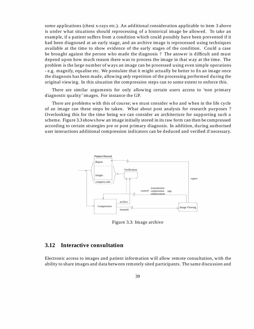
some applications (chest x-rays etc.). An additional consideration applicable to item 3 aboveis under what situations should reprocessing of a historical image be allowed. To take anexample, if a patient suffers from a condition which could possibly have been prevented if ithad been diagnosed at an early stage, and an archive image is reprocessed using techniquesavailable at the time to show evidence of the early stages of the condition. Could a casebe brought against the person who made the diagnosis ? The answer is difficult and mustdepend upon how much reason there was to process the image in that way at the time. Theproblem is the large number of ways an image can be processed using even simple operations- e.g. magnify, equalise etc. We postulate that it might actually be better to fix an image oncethe diagnosis has been made, allowing only repetition of the processing performed during theoriginal viewing. In this situation the compression steps can to some extent to enforce this.

There are similar arguments for only allowing certain users access to ‘non primarydiagnostic quality’ images. For instance the GP.

There are problems with this of course; we must consider who and when in the life cycleof an image can these steps be taken. What about post analysis for research purposes ?Overlooking this for the time being we can consider an architecture for supporting such ascheme. Figure 3.3 shows how an image initially stored in its raw form can then be compressedaccording to certain strategies pre or post primary diagnosis. In addition, during authoriseduser interactions additional compression indicators can be deduced and verified if necessary.

Patient Record

Compression

images

Report

Verification

compress inforeport

transmission compression enhancement

infocontrol

archive

transmitImage Viewing

Figure 3.3: Image archive

3.12 Interactive consultation

Electronic access to images and patient information will allow remote consultation, with theability to share images and data between remotely sited participants. The same discussion and

39

shared visual workspace that would occur in a normal face to face meeting can be reproducedwith enhancements performed by each user being shown on the display of the other as well.The concept has been investigated in other domains, and techniques such as the electronicwhite board have been used. We envisage the following for a medical consultation:

� Voice communication - essential.

� Shared images - very useful/essential.

� Graphical overlays on shared images, including labelling, ROI - very useful.

� Video-phone images of participants - possibly helpful.

The provision of real time voice and graphical (geometrical as distinct from image based)animation will be readily achieved over N-ISDN. As a live situation demands that extendedperiods of waiting for images to be transmitted is unacceptable then we must either transmitthe required images to any participants who do not have local access prior to the conversationtaking place, or alternatively reduce the volume of data to be transmitted by selection andcompression of the image content. One possibility will be to allow the ’speaker’ to controlthe content and compression directly by selection mechanisms or indirectly by highlightingROI areas, and thus enabling the higher quality requirements implied within the region tobe given to the compression module. In addition any information already known to thecompression module regarding image type and structure could be used improve efficiency.

3.13 Characteristics required from the compression scheme

From the previous sections we can conclude that a lossy compression scheme would ideallysupport some of the following features/ characteristics:

� Systems for consultation, emergency or remote teleradiology require a compressionscheme where the quality of images can be improved by sending more data.

� Variable quality across differing regions of an image.

� Variable size (high frequency filtered) images for use as SIM (spatial information models,icons) and for display on lower resolution monitors as review images, for GP’s use, andproviding zoom facilities (Bridgood & Staab, 1992).

� The computational load produced by the encoding/decoding should not be too great,although we will be satisfied if it would run in software on one of today’s reasonablypowerful workstations or perhaps with the addition of some inexpensive hardware, forinstance a Digital Signal Processor board.

40

Ideally the compression scheme would allow some or all of the parameters associated withthe above options to be specified at decode time. This will then allow a compressed imageto be uncompressed within a set of constraints, only requiring some of the information tobe accessed or transmitted to the (remote) decompression view station. Additionally someconstraints can be placed on the compression of the image to improve compression ratios, anobvious consequence being that this step cannot be reversed. As an example, if an image werecompressed within a specific region at lower quality then it would be impossible to improveon this quality for this region at decompression time. However for an image compressedto a high quality it would be possible to select only a section for decompression at highquality, thus saving time when transmitting the compressed image, of course the remainderof the image would be available at high quality if it were required, accepting the additionaltransmission time. The next chapter reports on the various schemes we have considered andoutlines a technique based on the recent mathematical theory of wavelets, for which encoderand decoder algorithms will be designed to support the desired characteristics.

3.14 Simplistic estimated compression ratios

An outline of a combination scheme to show how the various savings compound is describedusing estimates derived from inspection of example images. For any specific image theamount of compression which can actually be achieved will vary considerably dependingupon how well the image can be analysed.

Taking as an example a 2048�2048�12 chest x-ray image, 0 - 60% of the image isbackground (typical 25%) which is of no diagnostic value and can relatively easily be identifiedand subsequently be compressed to very high compression ratios. A 1024�1024 sized imagewill typically be displayed first prior to a zoom operation being applied (Kositpaiboon et al.,1989), enabling 75% of the remaining image to be disregarded. As it is unlikely that thefull 12 bit resolution can be resolved until some processing or intensity remapping has beenapplied to the image only 7-9 bits are initially required. For a specific diagnosis one region ofthe image invariably requires better or original quality than the rest which only provides thecontext for this ROI. If this region can be identified (see 3.10.2) then savings can be made inthe rest of the image.

It is important to note that the rest of the image would not appear significantly worse,it is more a case of not having some of the extra fine subjective detail which is importantfor some primary diagnoses (An image compressed to 10% has a typical signal/ noise ratio(SNR) of 38db which is still fairly good quality). By allowing some minute differences tooccur in an image however, large savings in the image representation size can be made. FromTable 3.3, for an image treated in this way we have reduction to 5% data volume for the initialimage reconstruction and this should still provide images of diagnostic quality in the requiredregions.

For progressive enhancement applications the initial selection images will be considerablysmaller still. The impact on transmission time requirements is clear; at 128K bit/s the original

41

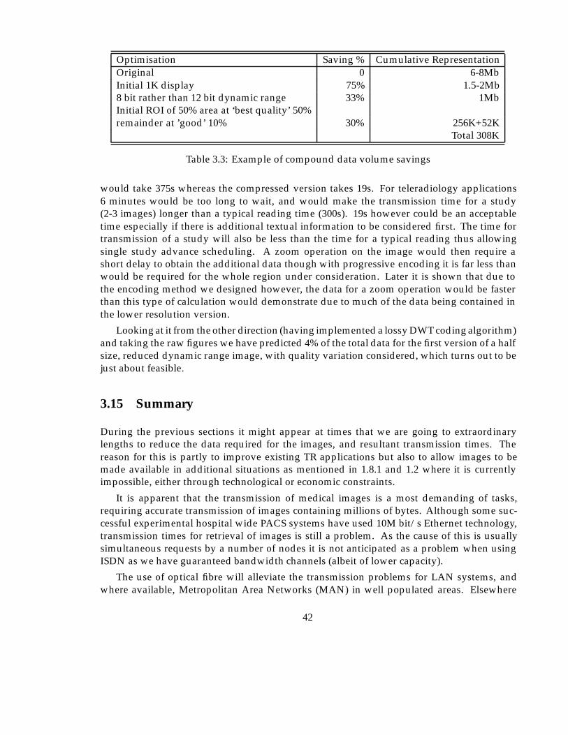
Optimisation Saving % Cumulative RepresentationOriginal 0 6-8MbInitial 1K display 75% 1.5-2Mb8 bit rather than 12 bit dynamic range 33% 1MbInitial ROI of 50% area at ‘best quality’ 50%remainder at ’good’ 10% 30% 256K+52K

Total 308K

Table 3.3: Example of compound data volume savings

would take 375s whereas the compressed version takes 19s. For teleradiology applications6 minutes would be too long to wait, and would make the transmission time for a study(2-3 images) longer than a typical reading time (300s). 19s however could be an acceptabletime especially if there is additional textual information to be considered first. The time fortransmission of a study will also be less than the time for a typical reading thus allowingsingle study advance scheduling. A zoom operation on the image would then require ashort delay to obtain the additional data though with progressive encoding it is far less thanwould be required for the whole region under consideration. Later it is shown that due tothe encoding method we designed however, the data for a zoom operation would be fasterthan this type of calculation would demonstrate due to much of the data being contained inthe lower resolution version.

Looking at it from the other direction (having implemented a lossy DWT coding algorithm)and taking the raw figures we have predicted 4% of the total data for the first version of a halfsize, reduced dynamic range image, with quality variation considered, which turns out to bejust about feasible.

3.15 Summary

During the previous sections it might appear at times that we are going to extraordinarylengths to reduce the data required for the images, and resultant transmission times. Thereason for this is partly to improve existing TR applications but also to allow images to bemade available in additional situations as mentioned in 1.8.1 and 1.2 where it is currentlyimpossible, either through technological or economic constraints.

It is apparent that the transmission of medical images is a most demanding of tasks,requiring accurate transmission of images containing millions of bytes. Although some suc-cessful experimental hospital wide PACS systems have used 10M bit/s Ethernet technology,transmission times for retrieval of images is still a problem. As the cause of this is usuallysimultaneous requests by a number of nodes it is not anticipated as a problem when usingISDN as we have guaranteed bandwidth channels (albeit of lower capacity).

The use of optical fibre will alleviate the transmission problems for LAN systems, andwhere available, Metropolitan Area Networks (MAN) in well populated areas. Elsewhere

42

basic rate ISDN is becoming available now, and should allow an enhancement of existingservices as well as new services. It is clear that even though ISDN is relatively fast (incomparison to the modem) transmitting large images is still far from instantaneous - Learspaper ‘Ultra high speed teleradiology with ISDN technology’ quotes 2min for a 1024�1024chest x-ray, which compared to 15min for transmission by 9600 baud modem is fast. Howeverthe situation can be worse than this with 2K2 and 4K2 images being typical for primarydiagnosis, often at 12 bits of dynamic range. The use of carefully applied compressiontechnology is therefore essential for some scenarios and, an extremely useful leveragingtechnology in others.

This chapter has attempted to show that a variety of requirements exist in terms of imageresolution, acceptable display speed, distortion and presentation method. Any or all of thesecan depend upon who the user of an image is, and why the image is being observed. Workingpractices also vary, and some technologies are better matched to particular working practices.The following chapter will concentrate on identification of a possible compression strategywhich can support as basic functions, many of the features identified in this chapter.

43

Chapter 4

Possible Compression Strategies

In this chapter we will consider the major alternative methods which have been utilised as thebasis of lossy image compression algorithms. The methods generally rely on a combinationof removing details which are less visible to the human eye, and modelling the specialclasses of two dimensional functions in which natural images are found, thus reducingredundancy/correlations within the image. The extension to progressive enhancementrequires algorithms which have a wide range of efficient compression ratios. These mustalso support the ability to add information to an image � to obtain an image �

0

with less error(according to whatever measure we are using). Ideally we should obtain the original imagein less than (or equal) to the original uncompressed image size.

It had already been decided that progressive enhancement would be an important tech-nique in reducing bandwidth and providing other facilities mentioned in 3.13 and that theserequire lossy compression techniques for the initial versions of an image.

The available lossy compression technologies were considered to find out how well (or if)the features identified in 3.13 could be supported. After some experimentation the wavelettransform was selected for further investigation.

4.1 Lossless compression

Early on in this work we decided not to utilise compression which is completely lossless inall respects, as the attainable ratios were not large enough to meet the ISDN requirements.However lossless techniques are used in the final stages of most lossy algorithms.

Images do not respond particularly well to statistical methods relying on skewed dis-tributions of pixel probability, for instance Huffman encoding and more recently arithmeticencoders. Runlength encoding of adjacent similar pixel values can be used, but in practice forgreyscale images runlengths are short, especially when the image contains noise. Differencingof adjacent pixel values works reasonably well as high frequency components with largedynamic range are uncommon, the distribution of difference values is therefore nonuniform

44

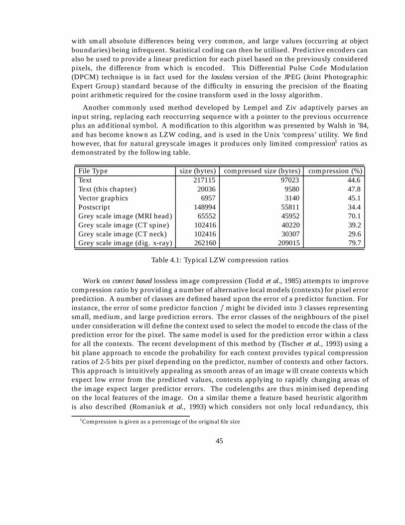
with small absolute differences being very common, and large values (occurring at objectboundaries) being infrequent. Statistical coding can then be utilised. Predictive encoders canalso be used to provide a linear prediction for each pixel based on the previously consideredpixels, the difference from which is encoded. This Differential Pulse Code Modulation(DPCM) technique is in fact used for the lossless version of the JPEG (Joint PhotographicExpert Group) standard because of the difficulty in ensuring the precision of the floatingpoint arithmetic required for the cosine transform used in the lossy algorithm.

Another commonly used method developed by Lempel and Ziv adaptively parses aninput string, replacing each reoccurring sequence with a pointer to the previous occurrenceplus an additional symbol. A modification to this algorithm was presented by Walsh in ’84,and has become known as LZW coding, and is used in the Unix ‘compress’ utility. We findhowever, that for natural greyscale images it produces only limited compression1 ratios asdemonstrated by the following table.

File Type size (bytes) compressed size (bytes) compression (%)Text 217115 97023 44.6Text (this chapter) 20036 9580 47.8Vector graphics 6957 3140 45.1Postscript 148994 55811 34.4Grey scale image (MRI head) 65552 45952 70.1Grey scale image (CT spine) 102416 40220 39.2Grey scale image (CT neck) 102416 30307 29.6Grey scale image (dig. x-ray) 262160 209015 79.7

Table 4.1: Typical LZW compression ratios

Work on context based lossless image compression (Todd et al., 1985) attempts to improvecompression ratio by providing a number of alternative local models (contexts) for pixel errorprediction. A number of classes are defined based upon the error of a predictor function. Forinstance, the error of some predictor function f might be divided into 3 classes representingsmall, medium, and large prediction errors. The error classes of the neighbours of the pixelunder consideration will define the context used to select the model to encode the class of theprediction error for the pixel. The same model is used for the prediction error within a classfor all the contexts. The recent development of this method by (Tischer et al., 1993) using abit plane approach to encode the probability for each context provides typical compressionratios of 2-5 bits per pixel depending on the predictor, number of contexts and other factors.This approach is intuitively appealing as smooth areas of an image will create contexts whichexpect low error from the predicted values, contexts applying to rapidly changing areas ofthe image expect larger predictor errors. The codelengths are thus minimised dependingon the local features of the image. On a similar theme a feature based heuristic algorithmis also described (Romaniuk et al., 1993) which considers not only local redundancy, this

1Compression is given as a percentage of the original file size

45

being attributed to smoothness within the image, but also global redundancy. Both typesof redundancy are based on dividing the image into small blocks of pixels and consideringthe small range of values within each block for local smoothness, and duplicate blocks forsimilarity. Typical compression from a scheme based on this technique was 2-6 bits perpixel, the authors claiming better compression ratios as compared to other lossless schemes.Certainly the idea of using heuristic feature models is appealing particularly where largenumbers of similar images are to be compressed, and could provide a worthwhile techniqueto be incorporated in our lossy schemes.

4.2 Lossy compression

4.2.1 Transform coding

Many different transformations have been used for image analysis and coding, they can begraded for compression efficiency according to their energy compaction ability. The objectiveis to obtain a set of coefficients which have a nonuniform distribution, with the majoritybeing negligible, the rest can then be quantized and losslessly encoded. Figure 4.2 showsa generic transform encoder, additional steps might be included for specific algorithms butall current encoders utilise this same basic approach. In general, the transform causes anincrease in representation size, either by an increase in number of coefficients as comparedto pixels in the original, and/or the coefficients having real rather than integer values. Anumber of factors must be considered including computational complexity, representationsize and relationship of coefficients to visual sensitivity. Figure 4.1 is a modified version of aprevious diagram (Ohta et al., 1992) and shows the major developments in transform coding.

4.2.2 Discrete cosine transform

The DCT has been popular for some time as a basis for lossy image compression, andincludes the well known baseline lossy JPEG encoder, which has become popular for generalimage compression tasks (Wallace, 1992; Wallace, 1991). It is closely related to the DiscreteFourier Transform, with the advantage of only producing real valued coefficients. Intensivecomputation is required to calculate the transform (even with ‘fast’ algorithms) and is usuallycarried out on individual ‘blocks’ of a subdivided image. It has two major drawbacks whenapplied to image coding:

Blocking effect. Quantization of low frequency coefficients produces horizontal and verticallines at the edges of each transform block. The cause of this is slight inaccuracy of theaverage colour of each block, which although only small is regular enough for the eyeto readily observe.

46

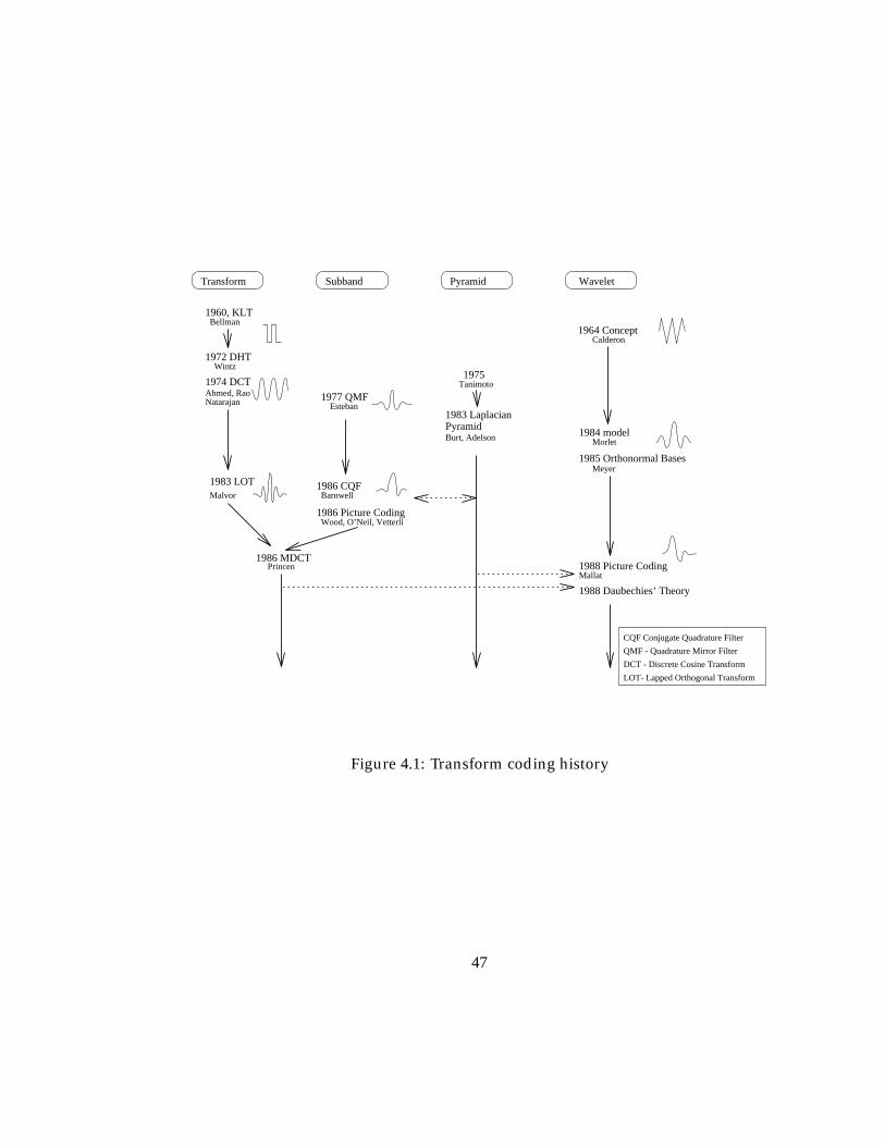
Transform

Wood, O’Neil, Vetterli1986 Picture Coding

Barnwell1986 CQF

1988 Picture CodingMallat

1988 Daubechies’ Theory

Princen

CQF Conjugate Quadrature Filter

QMF - Quadrature Mirror Filter

DCT - Discrete Cosine Transform

LOT- Lapped Orthogonal Transform

Subband Pyramid

1983 LOTMalvor

1960, KLTBellman

1972 DHTWintz

Calderon

1975Tanimoto

Esteban1977 QMF

1974 DCTAhmed, RaoNatarajan

1983 Laplacian PyramidBurt, Adelson

1964 Concept

1986 MDCT

Wavelet

Morlet1984 model

1985 Orthonormal BasesMeyer

Figure 4.1: Transform coding history

47

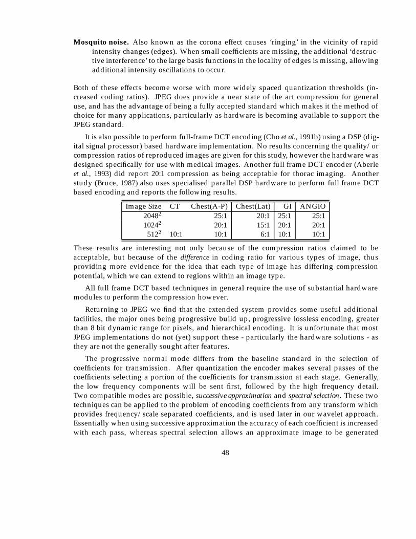
Mosquito noise. Also known as the corona effect causes ‘ringing’ in the vicinity of rapidintensity changes (edges). When small coefficients are missing, the additional ‘destruc-tive interference’ to the large basis functions in the locality of edges is missing, allowingadditional intensity oscillations to occur.

Both of these effects become worse with more widely spaced quantization thresholds (in-creased coding ratios). JPEG does provide a near state of the art compression for generaluse, and has the advantage of being a fully accepted standard which makes it the method ofchoice for many applications, particularly as hardware is becoming available to support theJPEG standard.

It is also possible to perform full-frame DCT encoding (Cho et al., 1991b) using a DSP (dig-ital signal processor) based hardware implementation. No results concerning the quality/orcompression ratios of reproduced images are given for this study, however the hardware wasdesigned specifically for use with medical images. Another full frame DCT encoder (Aberleet al., 1993) did report 20:1 compression as being acceptable for thorac imaging. Anotherstudy (Bruce, 1987) also uses specialised parallel DSP hardware to perform full frame DCTbased encoding and reports the following results.

Image Size CT Chest(A-P) Chest(Lat) GI ANGIO20482 25:1 20:1 25:1 25:110242 20:1 15:1 20:1 20:1

5122 10:1 10:1 6:1 10:1 10:1

These results are interesting not only because of the compression ratios claimed to beacceptable, but because of the difference in coding ratio for various types of image, thusproviding more evidence for the idea that each type of image has differing compressionpotential, which we can extend to regions within an image type.

All full frame DCT based techniques in general require the use of substantial hardwaremodules to perform the compression however.

Returning to JPEG we find that the extended system provides some useful additionalfacilities, the major ones being progressive build up, progressive lossless encoding, greaterthan 8 bit dynamic range for pixels, and hierarchical encoding. It is unfortunate that mostJPEG implementations do not (yet) support these - particularly the hardware solutions - asthey are not the generally sought after features.

The progressive normal mode differs from the baseline standard in the selection ofcoefficients for transmission. After quantization the encoder makes several passes of thecoefficients selecting a portion of the coefficients for transmission at each stage. Generally,the low frequency components will be sent first, followed by the high frequency detail.Two compatible modes are possible, successive approximation and spectral selection. These twotechniques can be applied to the problem of encoding coefficients from any transform whichprovides frequency/scale separated coefficients, and is used later in our wavelet approach.Essentially when using successive approximation the accuracy of each coefficient is increasedwith each pass, whereas spectral selection allows an approximate image to be generated

48

with only the low frequency coefficients, followed by improvements when high frequencycomponents are included. In this mode of operation AC prediction can be used to predictthe low frequency AC coefficients from the surrounding DC coefficients. This improvesthe quality of initial stages of progressive build up. We note this technique seems to sharecommon ground with the context based approach above, except that coefficients instead ofpixel values are being predicted.

The extended JPEG coder can provide a good number of the features which we require.Providing variable quality within an image is not specified but could be implemented on aper-block basis by adjusting the quality parameters for each block.

The Hierarchical mode of operation is provided by a sequence of filtering and samplingoperations when encoding. The image produced at each stage is then interpolated and used asa prediction for the next stage, the difference being encoded using the standard encoder. Thisintroduces a number of additional operations and appears to be rather a ‘bolt - on’ solution.

The JPEG standard does have a lossless mode of operation as mentioned earlier and itdoes provide good compression ratios given its lossless nature, however, it is not based onthe DCT and is a completely separate algorithm.

Experiments have been carried out to assess JPEG in the medical imaging field. Theresults (Kajiwara, 1992) reflect on the various practical advantages of compressing images,including reduction of transmission times, storage requirements (including floppy disks), andthe greater feasibility of long term archives. The summary concludes that 20:1 compressionfor 2K2 chest x-rays are acceptable to many researchers when using JPEG, although the finaluse of the images is not specified.

Image DataImage

Coefficients

Symbol

Sets

Transform QuantizingEncoding

Entropy

Binary

Representation

Figure 4.2: General transform coder

Other modifications have been made to the blocked DCT to remove the blocking artefacts,for instance a hierarchical approach requiring repeated encoding, decimation, and decodingoperations (Tan & Ghanbari, 1992). Although the resultant quality is better, especially withregard to these artefacts, the additional processing requirements creates severe limitations tothe implementation of such methods.

49

4.2.3 Subband coding

Subband coding was first introduced by John Woods (Woods, 1986) and is a closely relatedpredecessor to ‘wavelet’ based methods, being implemented using quadrature mirror filters(QMF) filters, and producing a specific number of band limited subbands, which are thenamenable to bit allocation techniques between the subsampled frequency bands. An adaptivetechnique was used to allocate bits within each band, bits being allocated between thesubbands to minimise the mean error (MSE) for DPCM coding of the subbands.

Subband coding for DSA images using non rectangular subband decompositions followedby DCT encoding of the subimages, has been implemented (Cetin, 1991) and results werepublished for compression ratios of 0.7 to 1.1 bpp. The paper unfortunately does not discussthe reasons for using this approach, and gives no indication of the acceptability of its use. Forcomparison the results of this experiment are plotted alongside our own results in chapter 7.

4.2.4 Vector quantization

The source image is divided into spatially contiguous blocks. These blocks are then mappedinto a vector set dimensionally similar to the block size. A codebook of representativevectors (codewords) is then generated using a clustering algorithm. Coding the imageconsists of finding the closest codeword for each given vector. This encoding methodgenerally provides poor compression ratios and can introduce significant visual artefacts to theimage. Enhancements have been made to Vector Quantization (VQ) including a hierarchicalprogressive algorithm (Wang & Goldberg, 1987) and a linear predictor technique usingmultiple level codebooks (Manikopoulos et al., 1989). Unfortunately neither provides thelevel of quality/compression of transform methods, although the progressive algorithm doeshave a mode of operation whereby errors are transferred from the low resolution to higherresolution images allowing lossless transmission of images at around 50% compression.

VQ has been applied to the problem of encoding medical image sequences (Sun &Goldberg, 1987). The method was chosen because these images have the special characteristicthat inter frame changes are from only two sources; the movement of the contrast agent, andbody movement. It is clear that VQ works well in this situation, particularly for representingthe body movement, but in general for a wider range of image types its application is morelimited.

4.2.5 Iterated function systems

Papers dealing with image coding using IFS or Fractal coding have been appearing for severalyears. We investigated these as a possible technique for application to medical images. Themethod which we investigated was originated by Michael Barnsley (Barnsley, 1988), but thiswork provided no automatic coding algorithm. A block based implementation (Jacquin,1990) was subsequently improved (Beaumont, 1991) involving the subdivision of the imageinto a number of blocks with multiscale matching on these blocks. We implemented a version

50

for which a brief description is subsequently given and applied it to some medical images.Finally we decided that the characteristics of such techniques did not quite fulfil our criterionfor the reasons outlined in section 4.2.5.3, and this technique was abandoned in preferencefor a wavelet based approach.

The technique is concerned with utilising the characteristic of many natural objects knownas self similarity. Artificial fractal objects can be constructed by iteratively applying a setof transformations. Often a small set of simple transformations can be used to generateincredibly complex functions (images). The major challenge for image coding is finding aset of transformations which will produce the desired image after iterative application. Oncesuch a set can be found then the required image can be completely represented by this set oftransformations thus producing a compressed representation.

Compression ratios of 1000’s:1 have been claimed for fractal techniques. However thishas been achieved by using the collage theorem (Barnsley, 1990) which involved operatorsmatching sections of an image by eye. The result was indeed to produce an extremely smallnumber of transformations which when applied could produce an image which appearssimilar to the original. The detail however will be very dissimilar to the original. We didnot consider this approach further due to this limitation although techniques to deducethe required transformations automatically will become available allowing the quality/compression ratio to be selected.

Another technique which does allow tighter control over the reconstruction errors pro-duced, is based on block matching within an image. We investigated Beaumont’s method(Beaumont, 1991) which was a development of another method (Jacquin, 1990). Apartfrom the high compression ratios claimed, an interesting feature of the implementation isthe computationally asymmetric encoder/decoder, with decoding requiring relatively fewoperations. Images could therefore be compressed off-line, at archive sites with powerfulmachines, allowing decoding and viewing at remote sites with the minimum of transmissionand processing overheads. We do not wish to provide a detailed description of the implemen-tation here, the next two sections provide a brief overview of the algorithm for the encodingand decoding processes.

4.2.5.1 Block based IFS encoding

The image is partitioned into domain blocks consisting of 8 � 8 pixel blocks. Each domainblock is subdivided into 4 � 4 pixel range blocks. To encode the image we require to find atransformation for each range block which will approximately map from one of the domainblocks. We used a minimum number of transformations consisting of:

� the compulsory height and width scaling by factor of half

� a grey level offset

� a grey level contraction

51

� an orthogonal reflection

The encoded representation of the image consists of the coefficients representing theseoperations plus the index of the domain block which provided the best match.

4.2.5.2 Block based IFS decoding

The image represented by this set of coefficients is decoded iteratively by starting with anarbitrary image and applying each transformation in turn, replacing each range block by theappropriately transformed domain block. The image converges to an approximation of theoriginal over a number of passes by a gradual reduction of the error contained within eachpixel. There is in fact an optimisation whereby the range block means are transmitted insteadof the grey level offset producing convergence in one iteration.

4.2.5.3 IFS summary

Following investigation, several characteristics were noted:

� The quality will vary within an image, depending upon how well the iteration of thetransform for each block converges to the required image. This is in turn related tothe number of possible transformations and the thoroughness (=time taken) for theencoding searches.

� A maximum quality limit for each allowable set of transformations is reached when nobetter matches are found.

� Larger images can in general be encoded to a better accuracy as there are more domainblocks. However if a free search of the entire image is allowed the block offset indiceshave a larger possible range, and may require greater storage requirements.

� Improvement in quality can also be made by allowing domain blocks to be positioned atany pixel position or to have a variety of sizes. The domain block index has greater rangeand the scaling factor is no longer implicit, respectively, decreasing the compressionratio.

� High frequency components generally have poorer matches producing errors andartefacts in the region of edges.

� The block match searching criterion can be adjusted to vary the quality/ compression/computational complexity.

� We could not envisage a way of selecting the quality for specific regions of an image.

52

In addition to these characteristics there is no direct support for progressive transmission, orproduction of variable resolution images. To enable a specific quality to be obtained we useda non fractal technique to store range blocks for which a sufficiently good match could notbe found. This does allow bounds to be kept on MSE for any required area of the image,although the number of blocks which are encoded by a fractal transformation rapidly dropsbeyond the ‘natural’ quality produced by the transform specification.

We concluded that IFS encoding has a number of problems which make it unsuitablefor use in medical image compression. In applications where only an impression of a sceneis required, rather than exact detail (e.g. photographic databases) there is the possibility offurther development, as is being performed by Iterated Systems Ltd, Atlanta.

In a recent paper, an experiment was performed using a similar block transform techniqueto compress MR images (Popescu & Yan, 1993) and concluded that quite good compressionratios were possible, this being partly due to the large areas of similar grey level intensitywithin these images. Other methods however, also benefit from this type of characteristicas few high frequency components are present within these areas. The main advantageidentified by the study was the fast decoding which is possible, providing a relatively weakoverall argument for its use.

4.2.6 Neural nets

Neural nets were considered next as a possible candidate for providing a compressionalgorithm. A multi layer network with input, hidden and output nodes is used. An image isdivided into blocks and the neural net is trained with a number of example blocks wherebythe internal weights are adjusted. An image is then compressed by using the values of thehidden node layer as the compressed representation of the image. To decompress the imageit is merely fed through to the output layer.

This simple but elegant technique has much appeal especially when we consider thespecialist nature of the images which are to be compressed, a different net could be trainedfor each type of image for instance - even for each area of anatomy. There are many possibleenhancements to such techniques for instance Marsi (Marsi & Carrelo, 1992) proposes asolution where a number of neural nets with differing numbers of hidden nodes are trainedfor each block. The net providing reconstruction of the required quality (SNR) is then chosen.The advantages of this is that ‘simple’ blocks require only a small net, and more complexblocks use larger nets, which obviously decrease compression ratio.

Finally, it was decided not to pursue the use of neural nets as a method of encodingmedical images at the present time due to the following:

Quality. It is not clear that very high quality can be achieved if required when compressionratio is relaxed. In addition, there was concern about spurious artefacts occurring incertain situations.

53

Black box. Unfortunately it is difficult to analyse the net to find out why or how a given com-pression was achieved. This will undoubtedly cause problems should the compressionfail in some respect.

Other features. It was not clear if or how features such as progressive enhancement or SIM’scould be catered for. Retrospectively we consider there are some possibilities in termsof hierarchical net structures, based on the observation that most of these features occurin the wavelet transform due to its hierarchical characteristics.

Nets representation. The compression ratios given in some articles do not include the storagerequired for the net itself. The assumption is that the net is available at the decoderand forms part of the algorithm itself. This implies that we would either have to definestandard nets or transmit alongside the coded image(s).

4.2.7 Wavelet transform

Wavelet coding can be considered as both transform and/or subband coding, since it can beimplemented as subband filter banks. A summary of the properties of the DWT are:

� Multi resolution.

� No artificial blocking required.

� Computationally relatively fast.

� Localisation (shorter basis for higher frequency).

� Compact energy spectrum.

� A directional component is included in the two dimensional transform allowing hori-zontal, vertical and ‘corner’ features to be identified from the coefficient set.

� Image ‘fingerprint’ is possible for efficient image indexing and identification.

The narrow filter orthogonal transform derived by Daubechies (Daubechies, 1988) waschosen as the basis of the coding method because of its good spatial localisation and rapidconvergence properties. The details of the transform and its implementation are provided inthe next chapter with a description of the encoding technique which we developed to allowthese properties to be utilised in chapter 6.

As might be expected, there are some disadvantages to the transform. Firstly to provide acomplete decomposition the original data set must have 2N , N 2 Z pixels in each dimensionand secondly the filter arithmetic includes irrational constants. Both of these problems areconsidered later in sections 5.5.2 and 5.5.3.

54

4.3 Specialist techniques

Most medical images are captured for a specific purpose, with particular processing require-ments. We believe that it is possible to utilise the multi resolution representation producedby the wavelet transform as the basis for further processing. In addition, the geometry ofimages can then be utilised to provide further coding efficiency. This is hinted at in a paper onradiographic image sequence coding using adaptive vector quantization (Sun & Goldberg,1987) where the results demonstrate that ‘good reproduction especially in those parts of theimage containing contrast agent, can be obtained at a compression ration of 10:1’ (italics added).We expect a number of techniques can be developed to locate the significant medical areasfor each type of image. This information can then be used by the general purpose multiresolution transform to more usefully allocate the bits in the compressed representation.

Three Dimensional or Multi slice images obviously contain inter frame correlations whichshould be exploited. These have not been considered in detail in this work but possibleenhancements to deal with this are discussed in chapter 9.

4.3.1 Hierarchical representations

Intuitively, a hierarchical representation appears to provide a good framework in which toperform image analysis. Initially, reduced (in both detail and size) images can be considered,with subsequent processing of the larger and more detailed versions restricted to ‘interesting’areas or specific features. This allows the image features to be considered in a structured way,and in context with the rest of the image. In this way the vast complexity of the completeimage with all its features, on a number of scales, can be overcome. We suggest that thisapproach will work at a number of levels of abstraction, from simple pixel operations such asarea segmentation, through to anatomic structure labelling.

4.3.2 ROI and heuristic feature models

The ability to vary image reconstruction error rates within the spatial extent of an image hasbeen proposed to provide additional compression. Assuming we have an algorithm whichallows this to occur, then a method is required to select the quality of regions within an image.Referring back to 3.10.2 the same two categories of ROI will be considered.

For the user defined ROI some information used during processing can be utilised forarchival (post primary diagnosis) by the compression algorithm. Regions which had zoomoperations or other manipulation functions applied require that the compression gives better(perfect) quality to them - to the extent that similar processing of the uncompressed versionwill not uncover artefacts. Other regions do not need to be perfect under manipulation.

Alternatively it is plausible that scenarios exist where is can be justified to ask the user todefine a ROI. For instance, in an on-line consultation situation a reasonable approach mightbe for the initiator (sender) to select the main region for consideration. We might consider the

55

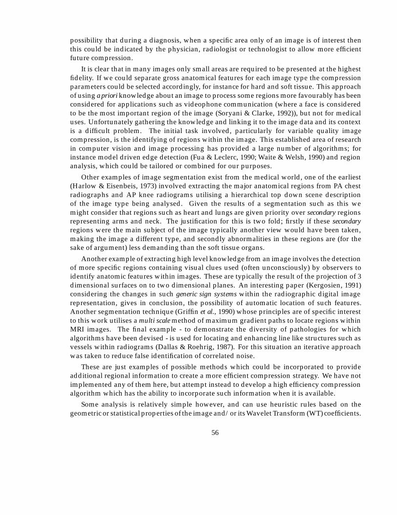
possibility that during a diagnosis, when a specific area only of an image is of interest thenthis could be indicated by the physician, radiologist or technologist to allow more efficientfuture compression.

It is clear that in many images only small areas are required to be presented at the highestfidelity. If we could separate gross anatomical features for each image type the compressionparameters could be selected accordingly, for instance for hard and soft tissue. This approachof using a priori knowledge about an image to process some regions more favourably has beenconsidered for applications such as videophone communication (where a face is consideredto be the most important region of the image (Soryani & Clarke, 1992)), but not for medicaluses. Unfortunately gathering the knowledge and linking it to the image data and its contextis a difficult problem. The initial task involved, particularly for variable quality imagecompression, is the identifying of regions within the image. This established area of researchin computer vision and image processing has provided a large number of algorithms; forinstance model driven edge detection (Fua & Leclerc, 1990; Waite & Welsh, 1990) and regionanalysis, which could be tailored or combined for our purposes.

Other examples of image segmentation exist from the medical world, one of the earliest(Harlow & Eisenbeis, 1973) involved extracting the major anatomical regions from PA chestradiographs and AP knee radiograms utilising a hierarchical top down scene descriptionof the image type being analysed. Given the results of a segmentation such as this wemight consider that regions such as heart and lungs are given priority over secondary regionsrepresenting arms and neck. The justification for this is two fold; firstly if these secondaryregions were the main subject of the image typically another view would have been taken,making the image a different type, and secondly abnormalities in these regions are (for thesake of argument) less demanding than the soft tissue organs.

Another example of extracting high level knowledge from an image involves the detectionof more specific regions containing visual clues used (often unconsciously) by observers toidentify anatomic features within images. These are typically the result of the projection of 3dimensional surfaces on to two dimensional planes. An interesting paper (Kergosien, 1991)considering the changes in such generic sign systems within the radiographic digital imagerepresentation, gives in conclusion, the possibility of automatic location of such features.Another segmentation technique (Griffin et al., 1990) whose principles are of specific interestto this work utilises a multi scale method of maximum gradient paths to locate regions withinMRI images. The final example - to demonstrate the diversity of pathologies for whichalgorithms have been devised - is used for locating and enhancing line like structures such asvessels within radiograms (Dallas & Roehrig, 1987). For this situation an iterative approachwas taken to reduce false identification of correlated noise.

These are just examples of possible methods which could be incorporated to provideadditional regional information to create a more efficient compression strategy. We have notimplemented any of them here, but attempt instead to develop a high efficiency compressionalgorithm which has the ability to incorporate such information when it is available.

Some analysis is relatively simple however, and can use heuristic rules based on thegeometric or statistical properties of the image and/or its Wavelet Transform (WT) coefficients.

56

As a demonstration of the possibility of regional selection the next section considers the easiestregion to identify.

4.3.3 Background removal

We have considered the idea of allowing different encoding characteristics for differentareas within the same image, with the aim of saving transmission bandwidth. One of thesimplest, most effective, and general possibilities is removal of the background which existsin many image types. Though the characterisation of the background will vary for imagetypes, the number of parameters required to allow it to be detected should be relativelylow, including perhaps some details of typical intensity, expected noise levels, and simplegeometric constraints. We would expect details such as these to be created for each image type,along with any specialist algorithms to create ‘plug in’ modules (or models) for the encoder.Defining sets of classes of images will thus allow better performance than could be obtainedby a general algorithm. By using both explicit information (e.g. typical background noiseof ndB for a certain image type), and implicit information (e.g. by specifying backgroundremoval), it is implied that this area makes no contribution to the diagnostic procedure to beperformed in the future.

For many images the background can be defined as a contiguous area of nearly uniformintensity. For each modality the intensity range of the background can be specified, typicallyblack or white. For specific views the start position for searches, for instance if region growingtechniques were used, could be configured. More sophisticated techniques have already beendeveloped for other applications. As an example we consider the energy minimising snakeas developed for separating human heads from background for model based videophoneapplications (Waite & Welsh, 1990). The wavelet transformation which we have used toprovide energy compaction within the image can also be utilised to provide a hierarchicalscheme for separating the subject from the background, described in section 6.8.2.

4.3.4 High frequency noise removal

In areas of continuous high or low intensity, uncorrelated small high frequency componentsof the image of comparable size to those identified as noise in the background (for each scale)are not visible, and could be disregarded as noise.

4.4 Summary

This chapter has attempted to give an outline of the major approaches to high efficiencycompression of images. We investigated and performed exploratory experiments for blockedDCT, Blocked IFS, and Wavelet approaches. The approach which supported the greatestnumber of the characteristics which were felt to be useful in supporting the facilities discussedin chapter 3 was the narrow filter orthogonal DWT.

57

Intensity Mapping

ROI

A

Background

removal (automatic)

Gradual Compression

Ratio Increase.

(might depend on

Annotation Marker(popup text or processing)

image geometry)

Radiologist Identified ROI12 bits dynamic range

8 bits deep equiv atextremities

A

Spatial Information Models

Figure 4.3: Sources of compression

With the good energy compaction capabilities of the DWT, combined with its frequency,and spatially represented coefficients, it will be possible to implement a scheme which caninclude the ideas in sections 3.14 and 4.3 as exemplified in figure 4.3.

58

Chapter 5

Wavelet Transforms

5.1 Important characteristics

Multiresolution representations of functions have been studied for use in image processing,computer vision and compression for many years. The advantages of this approach areobvious when we consider the vast numbers of discrete samples contained in the highresolution images capable of being captured and displayed by today’s technology. A fruitfulapproach when presented with such a vast quantity of data must be to extract the gross detailfrom the image, and using the results of this, to selectively process interesting areas in moredetail. Thus we have a hierarchical model of the image contents.

Several hierarchical decomposition algorithms have been devised for image coding in thepast but generally have the disadvantage of the details at different scales having significantcorrelation, thus providing a redundant representation. For some applications, this can haveadvantages, for example, the representation can be more resistant to arbitrary errors. Thewavelet transform, however, minimises the loss of information from one scale to the next, thusimproving analysis and compression capability. The orthogonal DWT can also distinguishbetween a number of spatial orientations, in particular the vertical and horizontal componentscan be used for further analysis of the image content. In addition a signature for an image(Wickerhauser, 1993) can be derived from the most energetic wavelet coefficients given theirfrequency, spatial, and orientation characteristics.

The Wavelet transform is computed by expanding a signal into a family of functionswhich are the dilation and translation of a single function called the wavelet basis (!(x)). Oneclass of wavelet basis (Daubechies, 1988) has been shown to be orthonormal and compactlysupported, providing both sharp localisation in space and frequency, together with efficientcomputational implementation.

One of the attractive properties of the discrete orthonormal wavelet transformation isthe possibility of an implementation by use of the recursive application of a series of filters.This technique has been well documented (Mallat, 1989; DeVore et al., 1992) and allows the

59

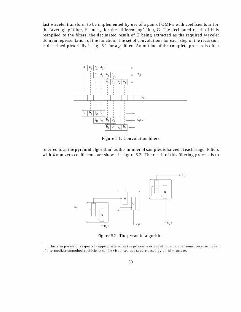
fast wavelet transform to be implemented by use of a pair of QMF’s with coefficients ak forthe ‘averaging’ filter, H and bk for the ‘differencing’ filter, G. The decimated result of H isreapplied to the filters, the decimated result of G being extracted as the required waveletdomain representation of the function. The set of convolutions for each step of the recursionis described pictorially in fig. 5.1 for a 2� filter. An outline of the complete process is often

s2

j-1

d2j-1

s2

j

b b b b

b b b b

b b b b

a a a a

a a a a

a a a a

0 1 2 3

0 1 2 3

321

321

321

321

Figure 5.1: Convolution filters

referred to as the pyramid algorithm1 as the number of samples is halved at each stage. Filterswith 4 non zero coefficients are shown in figure 5.2. The result of this filtering process is to

2-3

2-3

G

H

G

H

G

Hf(x)

S

DDD2

2-1

-2

Figure 5.2: The pyramid algorithm

1The term pyramid is especially appropriate when the process is extended to two dimensions, because the setof intermediate smoothed coefficients can be visualised as a square based pyramid structure.

60

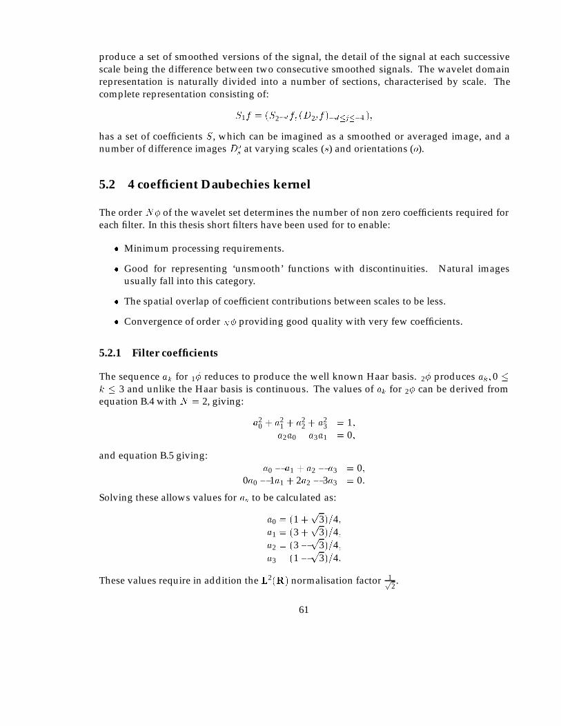
produce a set of smoothed versions of the signal, the detail of the signal at each successivescale being the difference between two consecutive smoothed signals. The wavelet domainrepresentation is naturally divided into a number of sections, characterised by scale. Thecomplete representation consisting of:

S1f = (S2�Jf; (D2jf)�J�j��1);

has a set of coefficients S, which can be imagined as a smoothed or averaged image, and anumber of difference images Do

sat varying scales (s) and orientations (o).

5.2 4 coefficient Daubechies kernel

The order N� of the wavelet set determines the number of non zero coefficients required foreach filter. In this thesis short filters have been used for to enable:

� Minimum processing requirements.

� Good for representing ‘unsmooth’ functions with discontinuities. Natural imagesusually fall into this category.

� The spatial overlap of coefficient contributions between scales to be less.

� Convergence of order N� providing good quality with very few coefficients.

5.2.1 Filter coefficients

The sequence ak for 1� reduces to produce the well known Haar basis. 2� produces ak; 0 �k � 3 and unlike the Haar basis is continuous. The values of ak for 2� can be derived fromequation B.4 with N = 2, giving:

a20 + a2

1 + a22 + a2

3 = 1;a2a0 + a3a1 = 0;

and equation B.5 giving:a0 � a1 + a2 � a3 = 0;

0a0 � 1a1 + 2a2 � 3a3 = 0:

Solving these allows values for an to be calculated as:

a0 = (1 +p

3)=4;a1 = (3 +

p3)=4;

a2 = (3�p

3)=4;a3 = (1�

p3)=4:

These values require in addition the L2(R) normalisation factor 1p2.

61

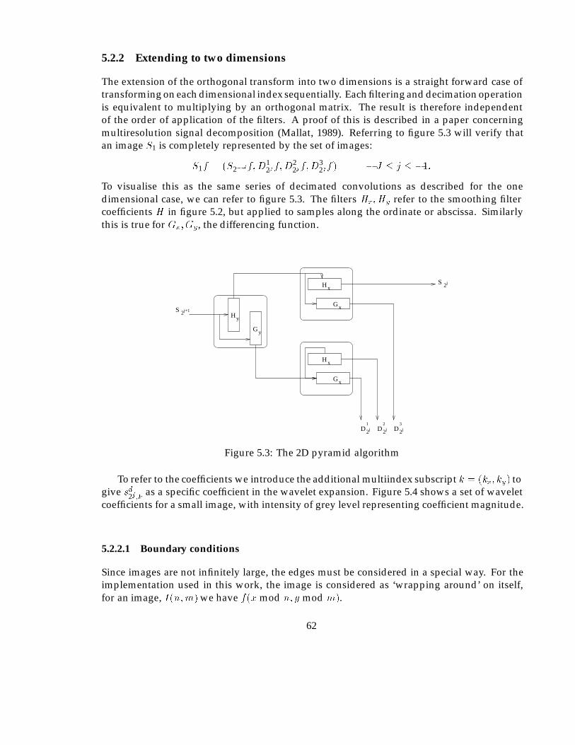
5.2.2 Extending to two dimensions

The extension of the orthogonal transform into two dimensions is a straight forward case oftransforming on each dimensional index sequentially. Each filtering and decimation operationis equivalent to multiplying by an orthogonal matrix. The result is therefore independentof the order of application of the filters. A proof of this is described in a paper concerningmultiresolution signal decomposition (Mallat, 1989). Referring to figure 5.3 will verify thatan image S1 is completely represented by the set of images:

S1f = (S2�Jf;D12jf;D

22jf;D

32jf) � J � j � �1:

To visualise this as the same series of decimated convolutions as described for the onedimensional case, we can refer to figure 5.3. The filters Hx; Hy refer to the smoothing filtercoefficients H in figure 5.2, but applied to samples along the ordinate or abscissa. Similarlythis is true for Gx; Gy, the differencing function.

S 2j

G

H

H

G

x

x

H

G

x

x

D2 D2

S 2j+1

jD2j j

y

y

1 2 3

Figure 5.3: The 2D pyramid algorithm

To refer to the coefficients we introduce the additional multiindex subscript k = (kx; ky) togive sd2j;k as a specific coefficient in the wavelet expansion. Figure 5.4 shows a set of waveletcoefficients for a small image, with intensity of grey level representing coefficient magnitude.

5.2.2.1 Boundary conditions

Since images are not infinitely large, the edges must be considered in a special way. For theimplementation used in this work, the image is considered as ‘wrapping around’ on itself,for an image, I(n;m) we have f(x mod n; y mod m).

62

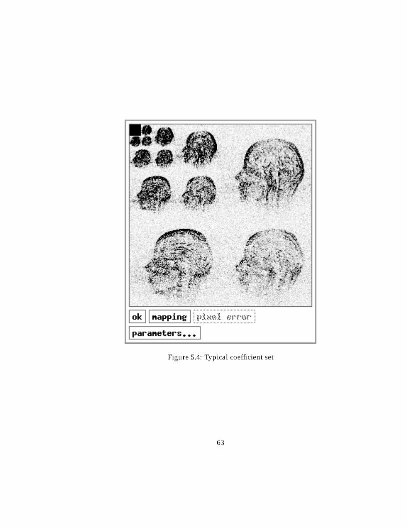
Figure 5.4: Typical coefficient set

63

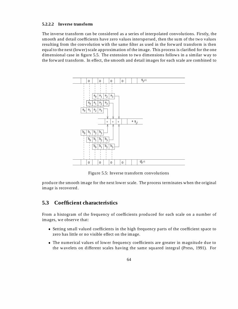
5.2.2.2 Inverse transform

The inverse transform can be considered as a series of interpolated convolutions. Firstly, thesmooth and detail coefficients have zero values interspersed, then the sum of the two valuesresulting from the convolution with the same filter as used in the forward transform is thenequal to the next (lower) scale approximation of the image. This process is clarified for the onedimensional case in figure 5.5. The extension to two dimensions follows in a similar way tothe forward transform. In effect, the smooth and detail images for each scale are combined to

s2

d2

j-1

j-1

+ s j2

+ ++

bbb

bbb

b b b b

a a a a

a a a a

a a a a

0 0 0 0

0 0 0 0

321

321

321

321

b321

b3210

0

0

0

0

0

Figure 5.5: Inverse transform convolutions

produce the smooth image for the next lower scale. The process terminates when the originalimage is recovered.

5.3 Coefficient characteristics

From a histogram of the frequency of coefficients produced for each scale on a number ofimages, we observe that:

� Setting small valued coefficients in the high frequency parts of the coefficient space tozero has little or no visible effect on the image.

� The numerical values of lower frequency coefficients are greater in magnitude due tothe wavelets on different scales having the same squared integral (Press, 1991). For

64

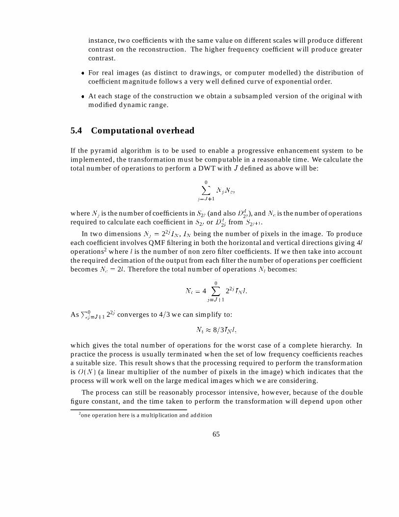
instance, two coefficients with the same value on different scales will produce differentcontrast on the reconstruction. The higher frequency coefficient will produce greatercontrast.

� For real images (as distinct to drawings, or computer modelled) the distribution ofcoefficient magnitude follows a very well defined curve of exponential order.

� At each stage of the construction we obtain a subsampled version of the original withmodified dynamic range.

5.4 Computational overhead

If the pyramid algorithm is to be used to enable a progressive enhancement system to beimplemented, the transformation must be computable in a reasonable time. We calculate thetotal number of operations to perform a DWT with J defined as above will be:

0Xj=J+1

NjNc;

whereNj is the number of coefficients inS2j (and alsoDd

2j), andNc is the number of operationsrequired to calculate each coefficient in S2j or Dd

2j from S2j+1.

In two dimensions Nj = 22jIN , IN being the number of pixels in the image. To produceeach coefficient involves QMF filtering in both the horizontal and vertical directions giving 4loperations2 where l is the number of non zero filter coefficients. If we then take into accountthe required decimation of the output from each filter the number of operations per coefficientbecomes Nc = 2l. Therefore the total number of operations Nt becomes:

Nt = 40X

j=J+1

22jIN l:

AsP0

j=J+1 22j converges to 4=3 we can simplify to:

Nt � 8=3IN l;

which gives the total number of operations for the worst case of a complete hierarchy. Inpractice the process is usually terminated when the set of low frequency coefficients reachesa suitable size. This result shows that the processing required to perform the transformationis O(N) (a linear multiplier of the number of pixels in the image) which indicates that theprocess will work well on the large medical images which we are considering.

The process can still be reasonably processor intensive, however, because of the doublefigure constant, and the time taken to perform the transformation will depend upon other

2one operation here is a multiplication and addition

65

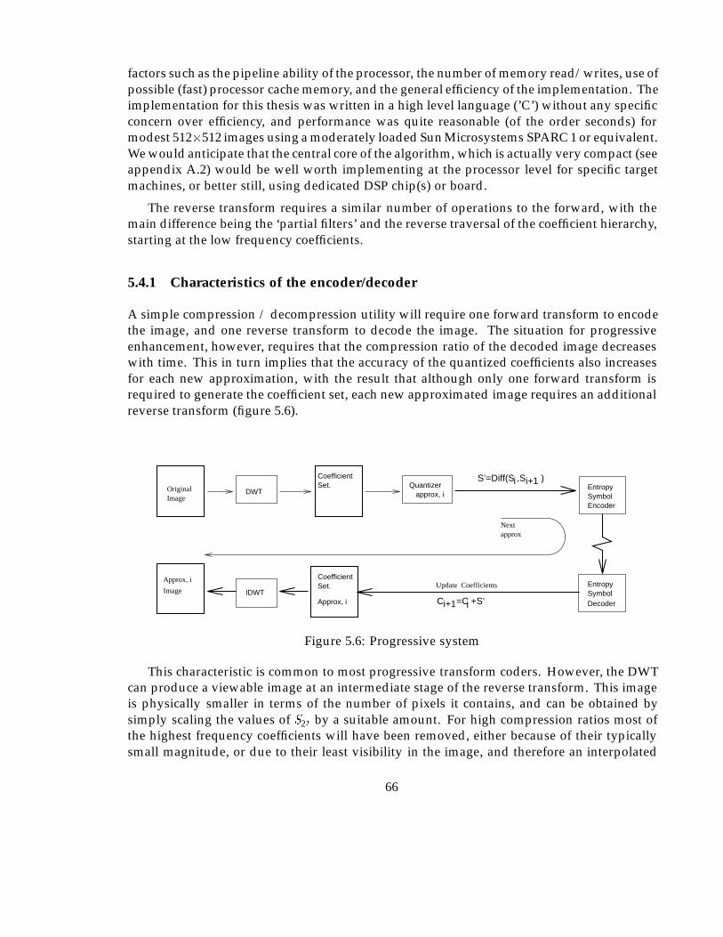
factors such as the pipeline ability of the processor, the number of memory read/writes, use ofpossible (fast) processor cache memory, and the general efficiency of the implementation. Theimplementation for this thesis was written in a high level language (’C’) without any specificconcern over efficiency, and performance was quite reasonable (of the order seconds) formodest 512�512 images using a moderately loaded Sun Microsystems SPARC 1 or equivalent.We would anticipate that the central core of the algorithm, which is actually very compact (seeappendix A.2) would be well worth implementing at the processor level for specific targetmachines, or better still, using dedicated DSP chip(s) or board.

The reverse transform requires a similar number of operations to the forward, with themain difference being the ‘partial filters’ and the reverse traversal of the coefficient hierarchy,starting at the low frequency coefficients.

5.4.1 Characteristics of the encoder/decoder

A simple compression / decompression utility will require one forward transform to encodethe image, and one reverse transform to decode the image. The situation for progressiveenhancement, however, requires that the compression ratio of the decoded image decreaseswith time. This in turn implies that the accuracy of the quantized coefficients also increasesfor each new approximation, with the result that although only one forward transform isrequired to generate the coefficient set, each new approximated image requires an additionalreverse transform (figure 5.6).

EncoderSymbolEntropy

Entropy SymbolDecoderC =C +S’i+1 i

OriginalImage

DWT

CoefficientSet.

Approx, iIDWTImage

Approx, i

CoefficientSet.

approx, iQuantizer

Nextapprox

Update Coefficients

iS’=Diff(S ,S )i+1

Figure 5.6: Progressive system

This characteristic is common to most progressive transform coders. However, the DWTcan produce a viewable image at an intermediate stage of the reverse transform. This imageis physically smaller in terms of the number of pixels it contains, and can be obtained bysimply scaling the values of S2j by a suitable amount. For high compression ratios most ofthe highest frequency coefficients will have been removed, either because of their typicallysmall magnitude, or due to their least visibility in the image, and therefore an interpolated

66

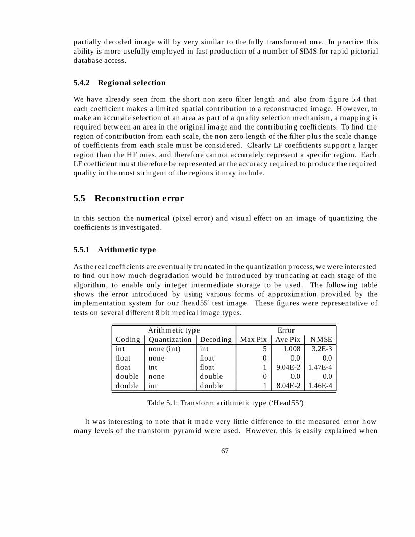
partially decoded image will by very similar to the fully transformed one. In practice thisability is more usefully employed in fast production of a number of SIMS for rapid pictorialdatabase access.

5.4.2 Regional selection

We have already seen from the short non zero filter length and also from figure 5.4 thateach coefficient makes a limited spatial contribution to a reconstructed image. However, tomake an accurate selection of an area as part of a quality selection mechanism, a mapping isrequired between an area in the original image and the contributing coefficients. To find theregion of contribution from each scale, the non zero length of the filter plus the scale changeof coefficients from each scale must be considered. Clearly LF coefficients support a largerregion than the HF ones, and therefore cannot accurately represent a specific region. EachLF coefficient must therefore be represented at the accuracy required to produce the requiredquality in the most stringent of the regions it may include.

5.5 Reconstruction error

In this section the numerical (pixel error) and visual effect on an image of quantizing thecoefficients is investigated.

5.5.1 Arithmetic type

As the real coefficients are eventually truncated in the quantization process, we were interestedto find out how much degradation would be introduced by truncating at each stage of thealgorithm, to enable only integer intermediate storage to be used. The following tableshows the error introduced by using various forms of approximation provided by theimplementation system for our ‘head55’ test image. These figures were representative oftests on several different 8 bit medical image types.

Arithmetic type ErrorCoding Quantization Decoding Max Pix Ave Pix NMSEint none (int) int 5 1.008 3.2E-3float none float 0 0.0 0.0float int float 1 9.04E-2 1.47E-4double none double 0 0.0 0.0double int double 1 8.04E-2 1.46E-4

Table 5.1: Transform arithmetic type (‘Head55’)

It was interesting to note that it made very little difference to the measured error howmany levels of the transform pyramid were used. However, this is easily explained when

67

we realise that the error contribution to the reconstructed image is the same regardless of theposition of the coefficient in the wavelet pyramid. Looking ahead to consider figure 6.2, we seeintuitively, that the coefficient magnitude though increasing with scale, is representing a largerarea of the original image, thus dividing the error between more pixels. Errors propagatedfrom one scale to the next are therefore not as one might initially expect, prone to ‘explode’. Adetailed analysis has subsequently been found (Chen et al., 1993), which continues to providea formula for total MSE (in the notation used previously where �k

jindicates the total error for

scale j, direction k) as follows:

�0 = ��J +

�1Xj=�J

3Xk=1

�k2j ;

thus indicating the total error is merely the sum of the component parts.

It was clear from these results that the intermediate storage of the coefficients should bein one of the floating point formats to allow for the best quality reproduction.

As there was some residual reconstruction error when the coefficients were rounded tointeger values, experimentation with rounding accuracy showed that rounding to the nearest0.25 (i.e. 2 bits past the binary point) reduces the reconstruction error to zero for images of 8bit dynamic range using one of the floating point forms.

5.5.2 Integer arithmetic

One alternative for this particular transformation was to note that the only source of nonintegers in the calculation are the

p2 and

p3 factors in the transform matrix. It would be

possible to perform the calculations in integer arithmetic keeping several integer values foreach coefficient to represent the various irrational multipliers. The number of individualinteger calculations increases by several times as does the required storage if the coefficientsgrow too large. There is scope for more investigation in to this possibility in the future, asperfect accuracy is maintained, although quantization will be required to prevent an increasein representation size.

This approach was abandoned as in the worst case the integer multipliers of the coefficientswill increase at around 5 extra bits per scale. As the final coefficients are quantized, and wehave found that keeping only two binary places provides an exact reproduction of the originalpixel values, some limited accuracy arithmetic should be possible.

5.5.3 Image size restrictions

The complete transform operates on data sets of 2n samples (n is a natural number), thoughn is not required to be the same for each dimension of an image. Many images are naturallyof these sizes, due to the digital nature of the imaging devices. For those that are not, wecan expand the image with the approximate background intensity (or black if this is not

68

clear). This will add virtually nothing to the encoded image due to the run-length encodingperformed in the final stages of the compression algorithm. Alternatively, if the originalimage size is stored with the encoded image, the positions of all zero coefficients relating tothe artificial border can be calculated, and ignored in the encoding algorithm.

5.5.4 Image processing in the wavelet domain

5.5.4.1 HF filtering and background removal

If we consider a typical radiographic image, there are many instances where a reasonablepercentage of the image is background, in the sense that it is outside of the object(s) underconsideration. This will appear on the image as a large area of similar intensity surroundingthe object. If this area was clean in the sense that it contained no noise (i.e. a single intensity),it would be compressed very efficiently by most compression algorithms. Unfortunately, thebackground area will usually contain some noise due to limitations of the imaging equipment,which thus reduces the efficiency of any high quality compression algorithm which attemptsto reproduce it. This type of typically high frequency ‘white noise’ is in fact the worst possiblesignal to compress as it is uncorrelated. Though there are other algorithms which couldseparate the areas we are interested in, the hierarchy of wavelet coefficients allows smallchanges in intensity at various scales to be removed. At larger scales the HF noise componentbecomes separated by a wider margin in terms of the magnitude of wavelet coefficients (figure5.7), thus making it easier to search for the image/ background boundary. The coefficients inthe background at higher scales can then be set to zero, thus improving the efficiency of thecompression. If required, the search in the region of the boundary can descend the hierarchyof coefficients to more accurately locate the boundary.

5.5.4.2 Intensity gradient and edge detection

The first step in most edge detection algorithms is noise filtering, followed by the production ofthe first and second differentials to locate the changes in intensity and their maxima/minima.Thresholding and linking then takes place to locate relevant edges. Considering a set ofdetail coefficients from the DWT, it is clear that the largest coefficient values for each scaleoccur in regions of more rapid intensity changes. It will, therefore, be possible to consider theproportion of each of the directional coefficient contributions in a specific region to determinethe possible strength and direction of a candidate edge. In addition, consideration can bemade of each scale and between adjacent scales to reinforce the location process. We hope inthe future to develop these ideas further.

5.5.5 Typical experimental result

Once the coefficients have been calculated, it remains to select, quantize, code, and store thesesuch that the decoding process can possess the characteristics we require. However, initial

69

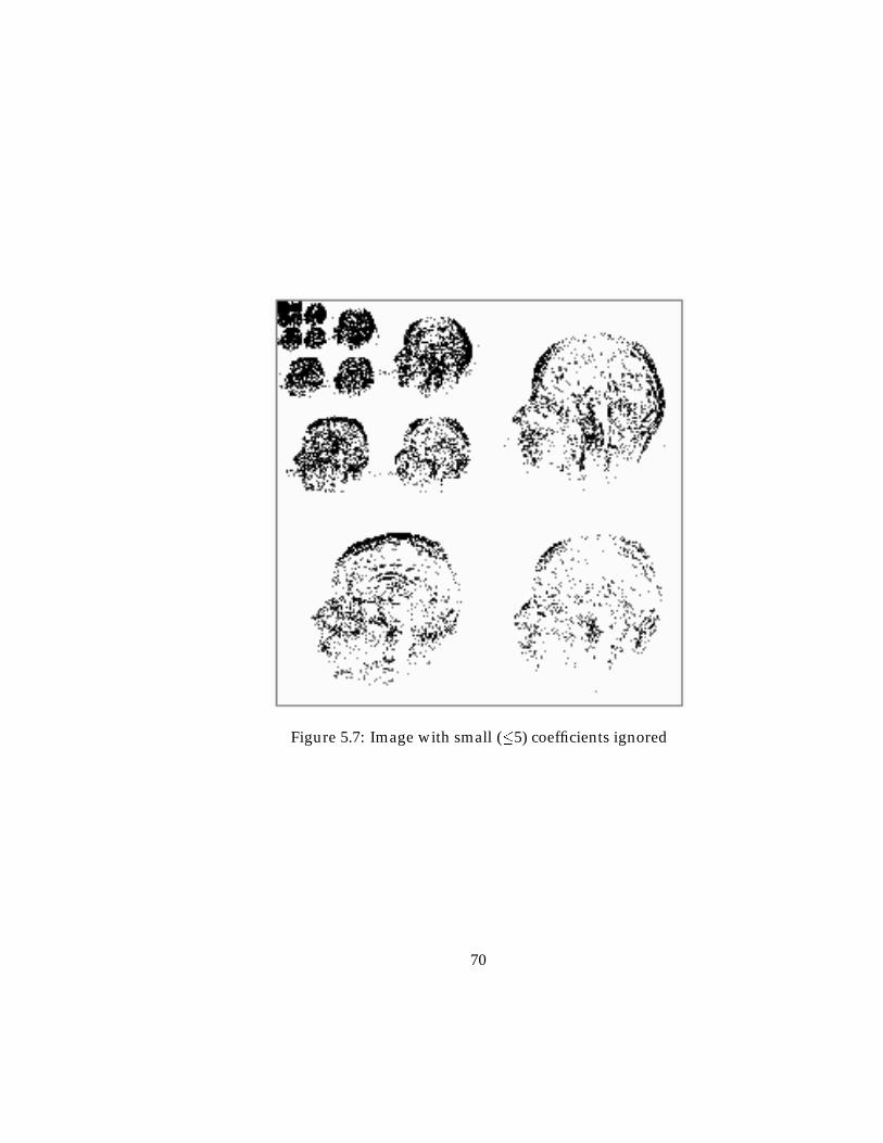
Figure 5.7: Image with small (�5) coefficients ignored

70

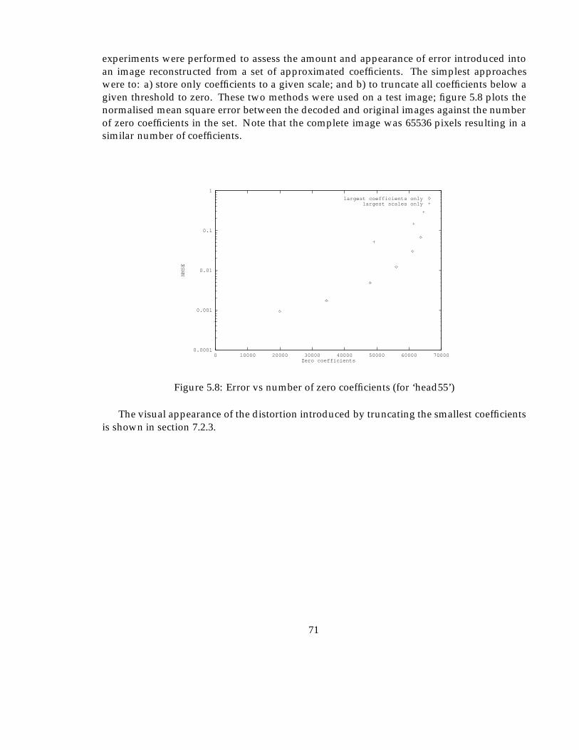
experiments were performed to assess the amount and appearance of error introduced intoan image reconstructed from a set of approximated coefficients. The simplest approacheswere to: a) store only coefficients to a given scale; and b) to truncate all coefficients below agiven threshold to zero. These two methods were used on a test image; figure 5.8 plots thenormalised mean square error between the decoded and original images against the numberof zero coefficients in the set. Note that the complete image was 65536 pixels resulting in asimilar number of coefficients.

0.0001

0.001

0.01

0.1

1

0 10000 20000 30000 40000 50000 60000 70000

NMSE

Zero coefficients

largest coefficients onlylargest scales only

Figure 5.8: Error vs number of zero coefficients (for ‘head55’)

The visual appearance of the distortion introduced by truncating the smallest coefficientsis shown in section 7.2.3.

71

Chapter 6

Coefficient Encoding Strategy

The objective of image compression is to reduce the number of bits of information requiredto represent the given set of pixels, whilst preserving the ‘best’ possible quality. Progressiveenhancement, introduces the additional complexity of selecting a method which allows thequality to increase with time and inclusion of additional bits of information. To be mosteffective, the early versions of an image must be the best possible quality, without precludingefficient further updates. To enable a quantization, and transmission strategy to be developed,some measure of the ’quality’ of a reconstructed image must be considered. Once this hasbeen decided upon we are then in a position to develop techniques which will minimise thereconstruction error of a compressed image, or minimise the reconstruction error with respectto time for the case of progressive enhancement.

It is worth noting that although the ability to vary the quality of different regions of eachimage is an important feature of the chosen method, the entire image is considered using thesame quality when evaluating compression ratios and effectiveness of the algorithms. Thisdecision is based on the observation that we require regional selection to be an additionalimprovement in quality for the selected regions. The base compression algorithm must beas effective as possible before regional selection and variable compression ratios are applied,and hence we need to compare with other non regional methods.

If the possibility exists of selecting regions requiring specific quality, then the reconstruc-tion error must include a measure of how accurately these regions were selected. This is aproblem in its own right of course as it depends entirely on the viewing characteristics of theobserver and the purpose for which the image will be reconstructed. An automated errormeasure is therefore not expected to be feasible.

Table 6.1 describes how the wavelet coefficients can be related to various image manipula-tion functions, user and window manager requests. These features can provide the frameworkfor both progressive enhancement and file compression algorithms. It is also interesting tonote that some image manipulation functions can be implemented more efficiently on thecompressed format than on a raw image. The details of this form of processing are left untilsection 6.9.

72

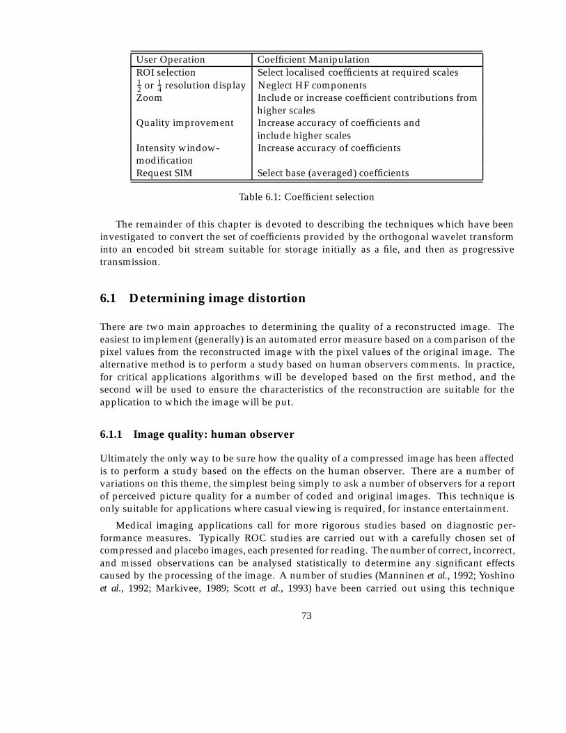
User Operation Coefficient ManipulationROI selection Select localised coefficients at required scales12 or 1

4 resolution display Neglect HF componentsZoom Include or increase coefficient contributions from

higher scalesQuality improvement Increase accuracy of coefficients and

include higher scalesIntensity window- Increase accuracy of coefficientsmodificationRequest SIM Select base (averaged) coefficients

Table 6.1: Coefficient selection

The remainder of this chapter is devoted to describing the techniques which have beeninvestigated to convert the set of coefficients provided by the orthogonal wavelet transforminto an encoded bit stream suitable for storage initially as a file, and then as progressivetransmission.

6.1 Determining image distortion

There are two main approaches to determining the quality of a reconstructed image. Theeasiest to implement (generally) is an automated error measure based on a comparison of thepixel values from the reconstructed image with the pixel values of the original image. Thealternative method is to perform a study based on human observers comments. In practice,for critical applications algorithms will be developed based on the first method, and thesecond will be used to ensure the characteristics of the reconstruction are suitable for theapplication to which the image will be put.

6.1.1 Image quality: human observer

Ultimately the only way to be sure how the quality of a compressed image has been affectedis to perform a study based on the effects on the human observer. There are a number ofvariations on this theme, the simplest being simply to ask a number of observers for a reportof perceived picture quality for a number of coded and original images. This technique isonly suitable for applications where casual viewing is required, for instance entertainment.

Medical imaging applications call for more rigorous studies based on diagnostic per-formance measures. Typically ROC studies are carried out with a carefully chosen set ofcompressed and placebo images, each presented for reading. The number of correct, incorrect,and missed observations can be analysed statistically to determine any significant effectscaused by the processing of the image. A number of studies (Manninen et al., 1992; Yoshinoet al., 1992; Markivee, 1989; Scott et al., 1993) have been carried out using this technique

73

to assess the effects of film versus CRT soft copy, and also to asses the effect of differingresolutions for various imaging applications. These results demonstrate, unsurprisingly, thatcertain types of abnormality require higher resolution/ dynamic range/ image processing fordiagnosis than others.

To assess the effect of compression or transmission techniques the control images must bepresented in a similar way to those under evaluation. For instance, it is misleading to compareresults for diagnosis of a compressed digitised x-ray with the original film, as we do no knowwhether any discrepancy is a feature of the compression process, or the digitisation process. Asimilar argument follows for display screen type, and environmental factors (lighting etc). Itis conceivable that studies of this nature would however be useful for checking the diagnosticefficacy of a complete system.

6.1.2 Image quality: error measures

When attempting to provide a numerical measure of the quality of a reconstructed imagethere are number of mathematical operators which can (and have) been used. The meansquare error (MSE) measure is most commonly found in the literature, but we can argue thatit does not necessarily provide the metric which most accurately matches the human visualsystem.

The situation becomes more complicated if we consider using a model of how the eyeand brain respond and process images. It is possible to build a model of such phenomena(Watson, 1987) and use this to measure the visibility of error introduced. If the model has beenused to produce the procedure which encoded the image however, it is not possible to use anerror measure based upon the model (otherwise we have not utilised the model properly) andhence there is still gives no guarantee that the model or compression actually does minimisevisual distortion. The only solution is to perform an empirical ROI study under carefullycontrolled conditions, to show statistically that the model and compression are valid.

We continue to utilise MSE and MAE (Mean Absolute Error) to provide a handle ondistortion, though we do not of course necessarily expect the parts of the system based uponthe models mentioned above to reduce these measures, though the apparent subjective qualitywill be improved.

6.2 Visual properties

We have two mechanisms for compressing images without producing visible artefacts in theuncompressed image. Accurate prediction or modelling of the image is one; matching theerror to the sensitivity of the human visual system is the other. Techniques from both ofthese approaches can be applied to the encoding of the wavelet coefficients. Taking a broaderview of the requirement for compression produces a third option - deliberately removingnonessential information - which will be considered later. The following sections describe

74

how we have used some of the well known human visual response characteristics to optimisethe quantization of coefficients.

There are two main effects used here:

Contrast sensitivity curve. Which makes use of the insensitivity of the eye to certain fre-quency components at low contrast.

Contrast masking. Uses the effect that high contrast regions tend to mask errors. Highcontrast or edges make small errors invisible or conversely low contrast areas highlighterrors. This effect can easily be seen on 8 bit colour displays when large areas of veryslight colour variation (e.g. clear sky views) show the colour quantization as bandingon screen.

6.3 Quantization characteristics

The storage requirements for the set of coefficients generated is greater than the original imagebecause anN �N integer pixel image produces N �N real coefficients at scale k and locationof support cj;k. To achieve a compression of the image the coefficients must be quantized.There are a number of possible alternatives while using the general strategy of preserving thelargest coefficients, as these have most visible effect on the image when it is reconstructed.In a progressive setting, adding coefficients from a higher scale we call spectral selection, andimproving the approximation of coefficients is termed successive approximation. The methodsconsidered are:

� Set all coefficients less than some value, l to zero. This approach was used earlier toproduce successive approximation for comparison with spectral selection.

� Uniform quantization by truncating each coefficient to the same accuracy. This is easilyachieved for some error rates by deleting the l least significant bits.

� Non-uniform quantization of coefficients at each scale to take advantage of the contrastmasking curve.

� Varying the base threshold of the quantizer at each scale, j and each orientation, o toutilise the contrast sensitivity curve (CST).

It is necessary to select the quantization scheme for each scale j. In the next few sections,a number of techniques are considered to help in the design of the quantizing method.

75

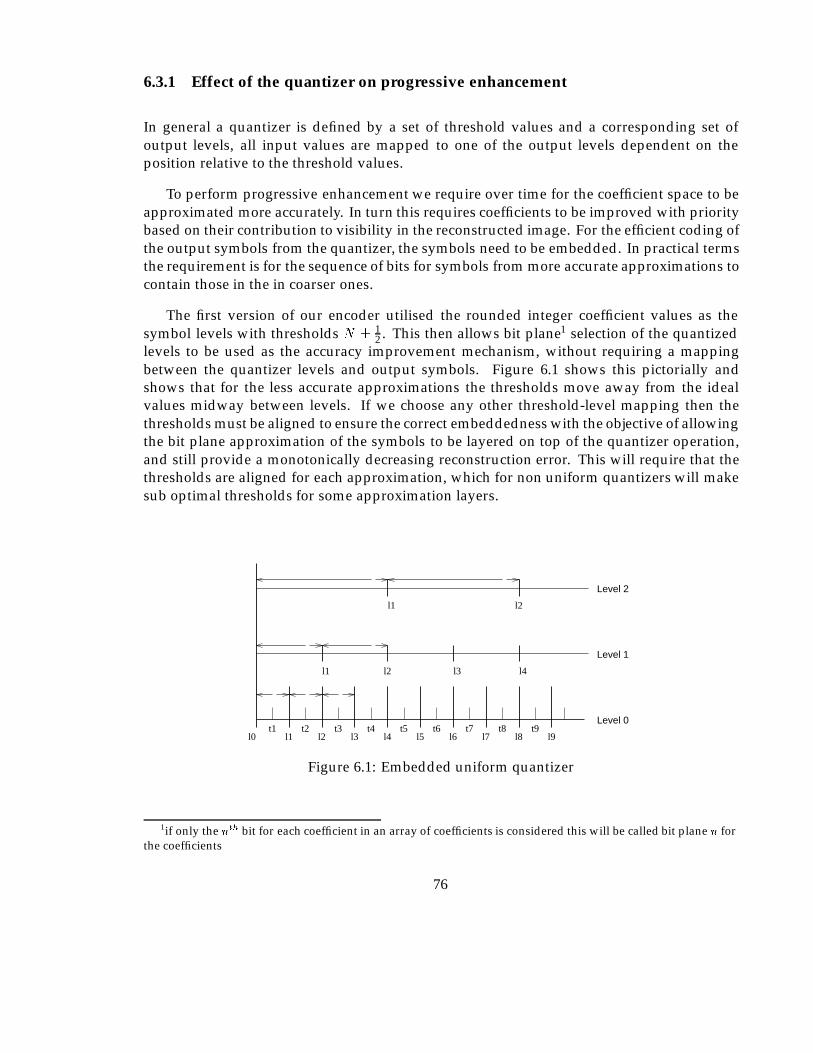
6.3.1 Effect of the quantizer on progressive enhancement

In general a quantizer is defined by a set of threshold values and a corresponding set ofoutput levels, all input values are mapped to one of the output levels dependent on theposition relative to the threshold values.

To perform progressive enhancement we require over time for the coefficient space to beapproximated more accurately. In turn this requires coefficients to be improved with prioritybased on their contribution to visibility in the reconstructed image. For the efficient coding ofthe output symbols from the quantizer, the symbols need to be embedded. In practical termsthe requirement is for the sequence of bits for symbols from more accurate approximations tocontain those in the in coarser ones.

The first version of our encoder utilised the rounded integer coefficient values as thesymbol levels with thresholds N � 1

2 . This then allows bit plane1 selection of the quantizedlevels to be used as the accuracy improvement mechanism, without requiring a mappingbetween the quantizer levels and output symbols. Figure 6.1 shows this pictorially andshows that for the less accurate approximations the thresholds move away from the idealvalues midway between levels. If we choose any other threshold-level mapping then thethresholds must be aligned to ensure the correct embeddedness with the objective of allowingthe bit plane approximation of the symbols to be layered on top of the quantizer operation,and still provide a monotonically decreasing reconstruction error. This will require that thethresholds are aligned for each approximation, which for non uniform quantizers will makesub optimal thresholds for some approximation layers.

l0 l2 l3l1 l4 l5 l6 l7 l8 l9t1 t2 t3 t4 t5 t6 t7 t8 t9

Level 2

l1 l2

l2

l3 l4

l1

Level 1

Level 0

Figure 6.1: Embedded uniform quantizer

1if only the nth bit for each coefficient in an array of coefficients is considered this will be called bit plane n forthe coefficients

76

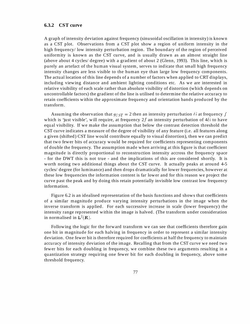
6.3.2 CST curve

A graph of intensity deviation against frequency (sinusoidal oscillation in intensity) is knownas a CST plot. Observations from a CST plot show a region of uniform intensity in thehigh frequency/low intensity perturbation region. The boundary of the region of perceiveduniformity is known as the CST curve, and is usually drawn as an almost straight line(above about 4 cycles/degree) with a gradient of about 2 (Glenn, 1993). This line, which ispurely an artefact of the human visual system, serves to indicate that small high frequencyintensity changes are less visible to the human eye than large low frequency components.The actual location of this line depends of a number of factors when applied to CRT displays,including viewing distance and ambient lighting conditions etc. As we are interested inrelative visibility of each scale rather than absolute visibility of distortion (which depends onuncontrollable factors) the gradient of the line is utilised to determine the relative accuracy toretain coefficients within the approximate frequency and orientation bands produced by thetransform.

Assuming the observation that gCST = 2 then an intensity perturbation �i at frequency f

which is ‘just visible’, will require, at frequency 2f an intensity perturbation of 4�i to haveequal visibility. If we make the assumption that below the contrast detection threshold theCST curve indicates a measure of the degree of visibility of any feature (i.e. all features alonga given (shifted) CST line would contribute equally to visual distortion), then we can predictthat two fewer bits of accuracy would be required for coefficients representing componentsof double the frequency. The assumption made when arriving at this figure is that coefficientmagnitude is directly proportional to reconstruction intensity accross the frequency space- for the DWT this is not true - and the implications of this are considered shortly. It isworth noting two additional things about the CST curve. It actually peaks at around 4-5cycles/degree (for luminance) and then drops dramatically for lower frequencies, however atthese low frequencies the information content is far lower and for this reason we project thecurve past the peak and by doing this retain potentially invisible low contrast low frequencyinformation.

Figure 6.2 is an idealised representation of the basis functions and shows that coefficientsof a similar magnitude produce varying intensity perturbations in the image when theinverse transform is applied. For each successive increase in scale (lower frequency) theintensity range represented within the image is halved. (The transform under considerationin normalised in L2(R).

Following the logic for the forward transform we can see that coefficients therefore gainone bit in magnitude for each halving in frequency in order to represent a similar intensitydeviation. One fewer bit is therefore required for coefficients at half the frequency to maintainaccuracy of intensity deviation of the image. Recalling that from the CST curve we need twofewer bits for each doubling in frequency, we combine these two arguments resulting in aquantization strategy requiring one fewer bit for each doubling in frequency, above somethreshold frequency.

77

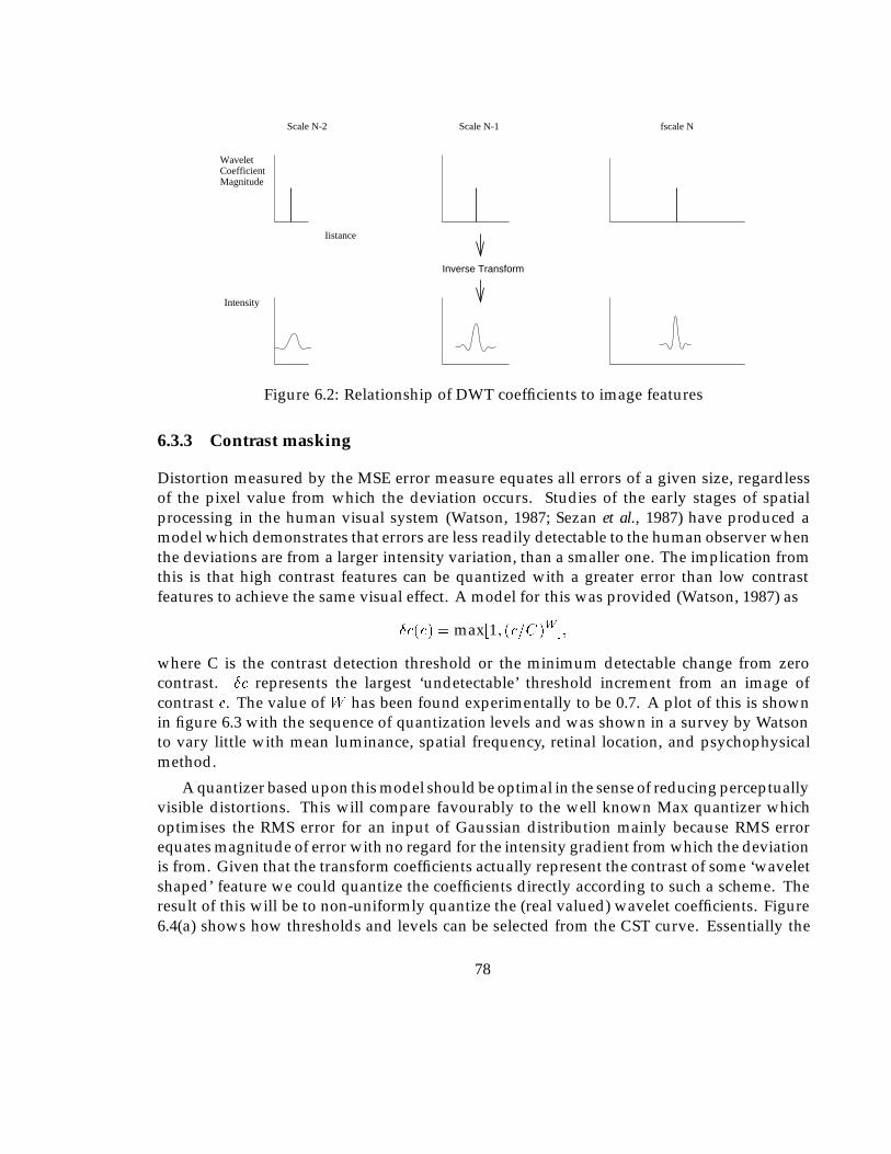
WaveletCoefficientMagnitude

Iistance

Scale N-1 fscale NScale N-2

Inverse Transform

Intensity

Figure 6.2: Relationship of DWT coefficients to image features

6.3.3 Contrast masking

Distortion measured by the MSE error measure equates all errors of a given size, regardlessof the pixel value from which the deviation occurs. Studies of the early stages of spatialprocessing in the human visual system (Watson, 1987; Sezan et al., 1987) have produced amodel which demonstrates that errors are less readily detectable to the human observer whenthe deviations are from a larger intensity variation, than a smaller one. The implication fromthis is that high contrast features can be quantized with a greater error than low contrastfeatures to achieve the same visual effect. A model for this was provided (Watson, 1987) as

�c(c) = max[1; (c=C)W ];

where C is the contrast detection threshold or the minimum detectable change from zerocontrast. �c represents the largest ‘undetectable’ threshold increment from an image ofcontrast c. The value of W has been found experimentally to be 0.7. A plot of this is shownin figure 6.3 with the sequence of quantization levels and was shown in a survey by Watsonto vary little with mean luminance, spatial frequency, retinal location, and psychophysicalmethod.

A quantizer based upon this model should be optimal in the sense of reducing perceptuallyvisible distortions. This will compare favourably to the well known Max quantizer whichoptimises the RMS error for an input of Gaussian distribution mainly because RMS errorequates magnitude of error with no regard for the intensity gradient from which the deviationis from. Given that the transform coefficients actually represent the contrast of some ‘waveletshaped’ feature we could quantize the coefficients directly according to such a scheme. Theresult of this will be to non-uniformly quantize the (real valued) wavelet coefficients. Figure6.4(a) shows how thresholds and levels can be selected from the CST curve. Essentially the

78

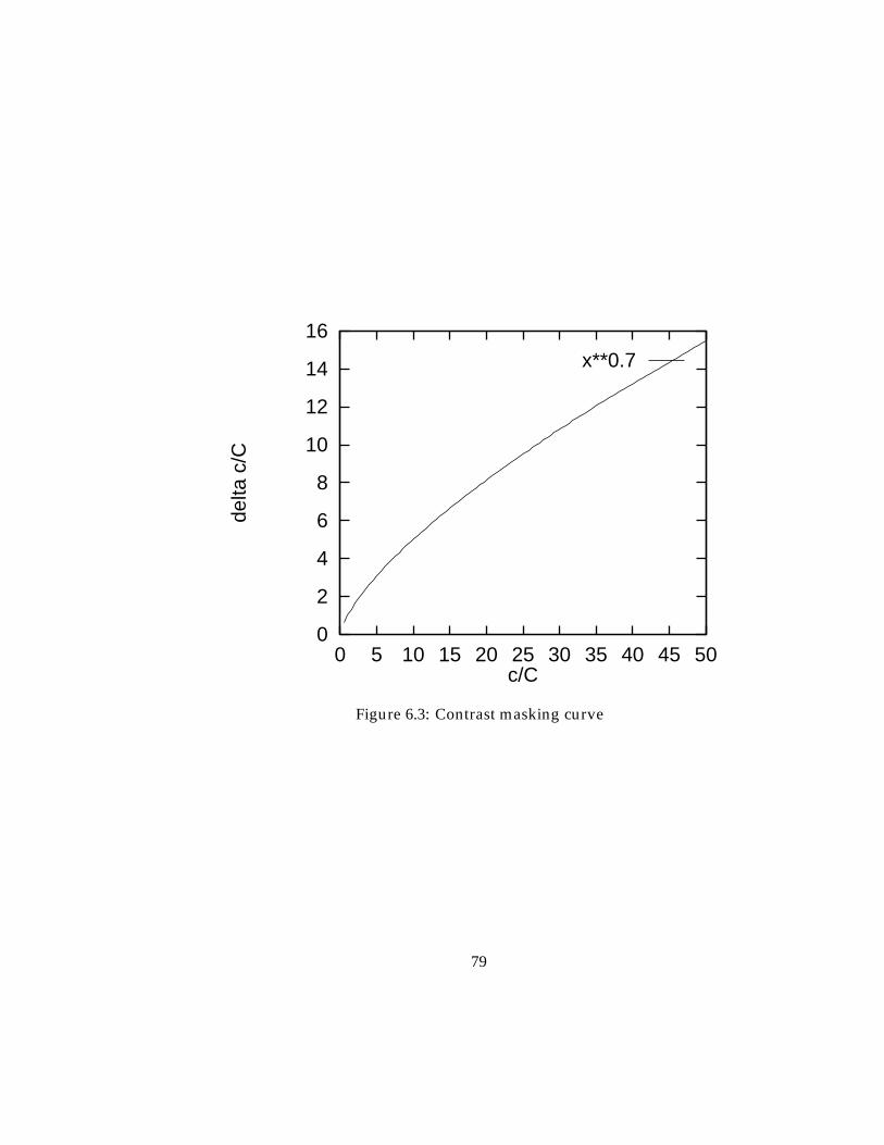
0

2

4

6

8

10

12

14

16

0 5 10 15 20 25 30 35 40 45 50

delta

c/C

c/C

x**0.7

Figure 6.3: Contrast masking curve

79

first threshold is set at the visibility threshold, thus ensuring that all values between L0 andT1 are quantized to L0 and are perceptually invisible. L1 must then also be no greater than thevisibility threshold from T1. At L1 a slightly greater quantization error can be accommodatedindicated by the vertical intersection with the curve, which is then projected along the contrastaxis to provide T2. The process continues to provide the required nonuniform quantizer.Once again, we can use this to optimise quality at a specific compression ratio by makingthe assumption that if the quantizer is set coarser than the visibility threshold then themagnitude of visible distortion from the range of quantized values will be approximatelysimilar. Put another way, we are assuming that the perceptual distortion produced byquantized coefficients will not be visibly greater between any pair of thresholds despitethe thresholds being separated by differing amounts. We will thus have an efficient system inthe sense that we will not have a large visible distortion in one component masking accuratereproduction in another.

This approach can be utilised for file compression where the quantization thresholds arestatic, however for progressive enhancement we have the problem of creating a non-uniformembedded quantizer. Though this is possible by aligning the thresholds (Elnahas et al., 1986)in a similar manner to the linear one in section 6.3.1. Some inefficiency is inevitable for allapproximations other that the one chosen to align to, and the symbols generated for eachlevel require mapping back to the original quantizer level values by the decoder, thus addingto the overall complexity.

c/C c/C

1

thresholdvisibility

T1

1

thresholdvisibility

L1L0 T2 L2 L0

inccontrast(norm)

c/Ccontrast (norm)

c/C

inccontrast(norm)

(a) (b)

10

contrast (norm)

symbol

zero contrast zero contrast

symbol 0

L2T1 T2

2 1

L2

2

T3

Figure 6.4: Contrast masking

An alternative is to restrict quantization levels and thresholds to integer values, thusallowing direct coding of the quantized values in figure 6.4(b). The new thresholds are alwayschosen to be closer together, thus ensuring that the only effect will be to slightly improve theworst quantization error of some levels. Depending on the final lossless encoding step theactual values of the levels might be used as input to a Huffman encoder as unused integers(symbols) will be ignored. Runlength encoding between bit planes however would not be

80

efficient without mapping to a reduced symbol set.

6.4 File compression

The following sections follow the development of our algorithm. The first version (I) formsthe basis on which a number of modifications are then made to enable the additional featureswe require to be incorporated.

This first version can only support progressive enhancement in the form of adding all theinformation from complete scales of the transform, which was shown in figure 5.8 to be poorin terms of the MSE at low and medium coding ratios. The method is ideal for non interactivefile compression as it is the least processor intensive.

The process for encoding an image to a file at a given compression ratio for storage consistsof the following steps:

1. Convert the pixel values into an array of values suitable for the transformation to operateon, we used the ‘C’ language floating point type float. It is possible that fixed point, oreven integer with assumed divisor factors, can be used if the minimum quantizationseparation of the coder is known, in which case the maximum accuracy required can becalculated.

2. Perform the forward (DWT) transform for DAUB4 so that each pixel value becomesreplaced by a real valued coefficient.

3. Quantization strategies are applied, utilising the characteristics of the transformation toproduce a symbol set.

4. The resulting symbols are entropy encoded to remove statistical redundancy.

5. The bitstream plus any additional information, for instance coding tables, and headerinformation is written to a file.

Steps 1 and 2 are covered in previous chapters, step 3 has been introduced but will beanalysed in more detail subsequently and 4 is the subject of the next sections.

6.4.1 Quantization

The simplest form of quantization is a linear quantizer with thresholds at the points midwaybetween successive integers, and levels therefore at integer values. Section 7.2 uses the ‘C’round function to achieve this.

81

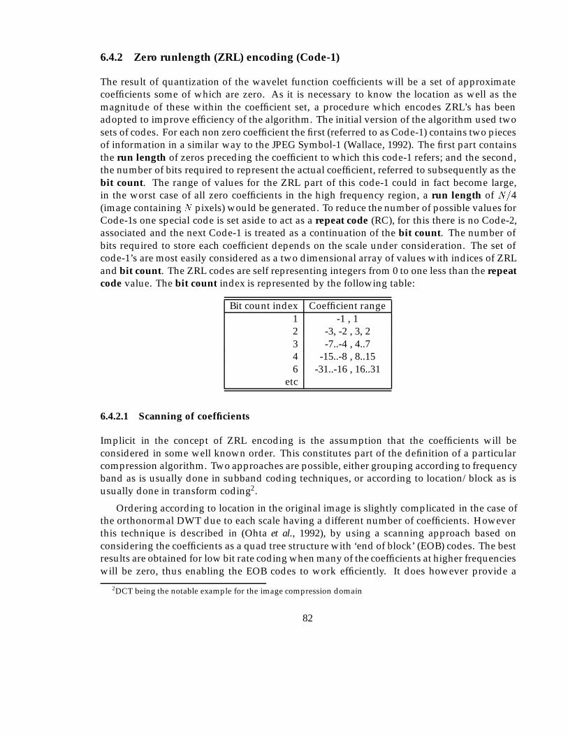
6.4.2 Zero runlength (ZRL) encoding (Code-1)

The result of quantization of the wavelet function coefficients will be a set of approximatecoefficients some of which are zero. As it is necessary to know the location as well as themagnitude of these within the coefficient set, a procedure which encodes ZRL’s has beenadopted to improve efficiency of the algorithm. The initial version of the algorithm used twosets of codes. For each non zero coefficient the first (referred to as Code-1) contains two piecesof information in a similar way to the JPEG Symbol-1 (Wallace, 1992). The first part containsthe run length of zeros preceding the coefficient to which this code-1 refers; and the second,the number of bits required to represent the actual coefficient, referred to subsequently as thebit count. The range of values for the ZRL part of this code-1 could in fact become large,in the worst case of all zero coefficients in the high frequency region, a run length of N=4(image containingN pixels) would be generated. To reduce the number of possible values forCode-1s one special code is set aside to act as a repeat code (RC), for this there is no Code-2,associated and the next Code-1 is treated as a continuation of the bit count. The number ofbits required to store each coefficient depends on the scale under consideration. The set ofcode-1’s are most easily considered as a two dimensional array of values with indices of ZRLand bit count. The ZRL codes are self representing integers from 0 to one less than the repeatcode value. The bit count index is represented by the following table:

Bit count index Coefficient range1 -1 , 12 -3, -2 , 3, 23 -7..-4 , 4..74 -15..-8 , 8..156 -31..-16 , 16..31

etc

6.4.2.1 Scanning of coefficients

Implicit in the concept of ZRL encoding is the assumption that the coefficients will beconsidered in some well known order. This constitutes part of the definition of a particularcompression algorithm. Two approaches are possible, either grouping according to frequencyband as is usually done in subband coding techniques, or according to location/block as isusually done in transform coding2.

Ordering according to location in the original image is slightly complicated in the case ofthe orthonormal DWT due to each scale having a different number of coefficients. Howeverthis technique is described in (Ohta et al., 1992), by using a scanning approach based onconsidering the coefficients as a quad tree structure with ‘end of block’ (EOB) codes. The bestresults are obtained for low bit rate coding when many of the coefficients at higher frequencieswill be zero, thus enabling the EOB codes to work efficiently. It does however provide a

2DCT being the notable example for the image compression domain

82

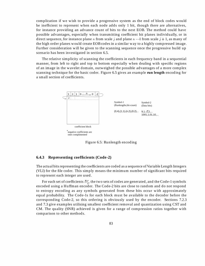
complication if we wish to provide a progressive system as the end of block codes wouldbe inefficient to represent when each node adds only 1 bit, though there are alternatives,for instance providing an advance count of bits to the next EOB. The method could havepossible advantages, especially when transmitting coefficient bit planes individually, or indirect sequence, for instance plane n from scale j and plane n� 1 from scale j+ 1, as many ofthe high order planes would create EOB codes in a similar way to a highly compressed image.Further consideration will be given to the scanning sequence once the progressive build upscenario has been investigated in section 6.5.

The relative simplicity of scanning the coefficients in each frequency band in a sequentialmanner, from left to right and top to bottom especially when dealing with specific regionsof an image in the wavelet domain, outweighed the possible advantages of a more complexscanning technique for the basic coder. Figure 6.5 gives an example run length encoding fora small section of coefficients.

*

ones complimentednegative coefficients are

Symbol-1

(0,4),(1,1),(n,2),(0,2),..

Symbol-2(Data bits)

1001,1,01,10,...

*

(Runlengths,bit-count)

9,1,-2,2,...

1 0 09 0 -2n

2

coefficient block

Figure 6.5: Runlength encoding

6.4.3 Representing coefficients (Code-2)

The actual bits representing the coefficients are coded as a sequence of Variable Length Integers(VLI) for the file coder. This simply means the minimum number of significant bits requiredto represent each integer are used.

For each set of coefficientsDo

2j the two sets of codes are generated, and the Code-1 symbolsencoded using a Huffman encoder. The Code-2 bits are close to random and do not respondto entropy encoding as any symbols generated from these bits occur with approximatelyequal probability. The Code-1s for each block must be available to the decoder before thecorresponding Code-2, so this ordering is obviously used by the encoder. Sections 7.2.3and 7.3 give examples utilising smallest coefficient removal and quantization using CST andCM. The quality (SNR) achieved is given for a range of compression ratios together withcomparison to other methods.

83

6.5 Progressive transmission

To allow progressive build up of an image it is necessary to provide successive approximationof coefficients. Although the most obvious method is spectral selection with a sequence ofreconstructions including coefficients from the next higher frequency band, the quality ofthe images is poor initially, with blocking artefacts producing a ‘low resolution’ effect. Thissubjective effect is noted in (DeVore et al., 1992) where it is shown that the rate of decay oferror in the reconstructed image will be sharper for coefficients considered in order of sizethan those considered in fixed lexicographical order. This effect was also presented in theprevious chapter.

So far we have considered only producing the best quality image in the shortest length oftime (fewest bits/coefficients). For the application areas under consideration in this thesis,we must also determine how user interactions as discussed in the latter sections of chapter 3can be supported. The selection of a ROI and its increase in priority in the transmission willrequire the set of coefficients contributing the required area to be identified. Zoom operationswill require additional coefficients to be considered and intensity windowing will requirecoefficients to be transmitted more accurately.

6.5.1 Sequential bit plane encoding

To enable the accuracy of coefficients to be gradually increased each additional improvementin accuracy is gained by reducing quantizer threshold distances. In terms of the linear integerquantizer discussed earlier, all that is required is extra bits of accuracy to all of the non zerocoefficients for each plane. Whilst this works well to reduce the number of bits required forCode-2’s for an initial estimate of an image including information from several scales, theCode-1’s must still all be transmitted in advance. To avoid this, the Code-1 was adjusted sothat each value of coefficient size (in bits) is treated in a separate pass, thus the coefficient sizecan be dropped from the Code-1, which is left as a simple run length value. It is now possibleto build up the coefficient bit counts gradually as required. Apart from the repeat codesrequired for very long run lengths, there is one code required for each non zero coefficientin both approaches. The run lengths will on average be longer for the progressive approach,however as no bit count is required. Figure 6.6 shows this for a small section of somecoefficient space.

It is now possible to produce a coded sequence of bits representing approximate valuesfor the largest valued coefficients initially. Subsequently, including more data will includeapproximations for smaller magnitude coefficients, and improve the accuracy of the largerones.

We now consider the efficiency of the new ordering. The number of Code-2 data bits willnot be changed since each coefficient retains the same representation - only the ordering of thebits is changed. The number and distribution of run length symbols for the new ordering isless obvious. For an image �, Nc(x) is defined as the number of coefficients of each quantized

84

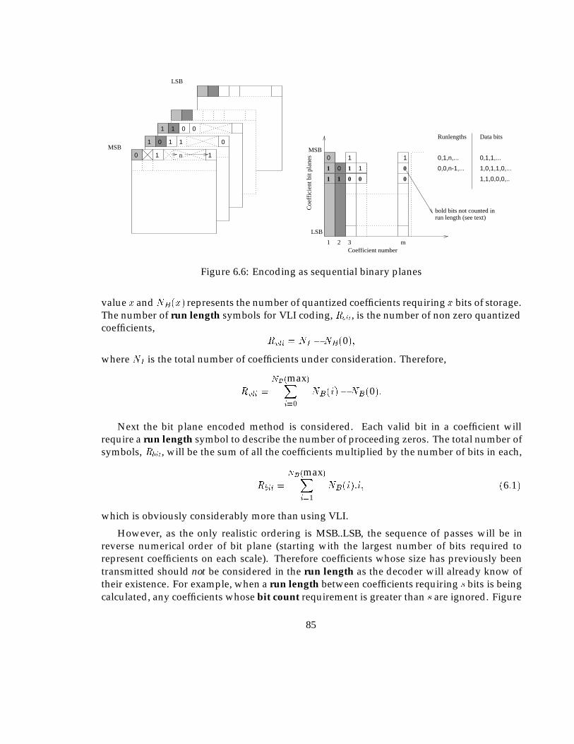
MSB0 1 n

1 0 1

1

01

1 1 0 0

LSB

Data bits

0

0

1

1

1

Runlengths

0,1,n,...

0,0,n-1,...

0,1,1,...

1,0,1,1,0,...

1,1,0,0,0,..

1

1 1 0

1

0

0

0

Coefficient number1 2 3 m

LSB

MSB

bold bits not counted inrun length (see text)

Coe

ffic

ient

bit

plan

es

Figure 6.6: Encoding as sequential binary planes

value x andNB(x) represents the number of quantized coefficients requiring x bits of storage.The number of run length symbols for VLI coding, Rvli, is the number of non zero quantizedcoefficients,

Rvli = NI �NB(0);

where NI is the total number of coefficients under consideration. Therefore,

Rvli =

NB(max)Xi=0

NB(i)�NB(0):

Next the bit plane encoded method is considered. Each valid bit in a coefficient willrequire a run length symbol to describe the number of proceeding zeros. The total number ofsymbols, Rbit, will be the sum of all the coefficients multiplied by the number of bits in each,

Rbit =

NB(max)Xi=1

NB(i):i; (6:1)

which is obviously considerably more than using VLI.

However, as the only realistic ordering is MSB..LSB, the sequence of passes will be inreverse numerical order of bit plane (starting with the largest number of bits required torepresent coefficients on each scale). Therefore coefficients whose size has previously beentransmitted should not be considered in the run length as the decoder will already know oftheir existence. For example, when a run length between coefficients requiring s bits is beingcalculated, any coefficients whose bit count requirement is greater than s are ignored. Figure

85

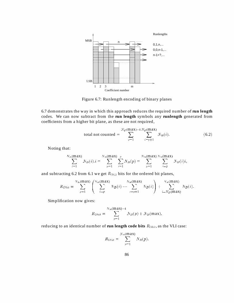
Coefficient number1 2 3 m

LSB

MSB n

Runlengths

0,1,n,...

0,0,n-1,...

n-1+?,...

Figure 6.7: Runlength encoding of binary planes

6.7 demonstrates the way in which this approach reduces the required number of run lengthcodes. We can now subtract from the run length symbols any runlength generated fromcoefficients from a higher bit plane, as these are not required,

total not counted =

NB(max)�1Xp=1

NB(max)Xi=p+1

NB(i): (6:2)

Noting that:

NB(max)Xi=1

NB(i):i �NB(max)X

p=1

pXi=1

NB(p) �NB(max)X

p=1

NB(max)Xi=p

NB(i)i;

and subtracting 6.2 from 6.1 we get RObit bits for the ordered bit planes,

RObit =

NB(max)Xp=1

0@NB(max)X

i=p

NB(i)�NB(max)Xi=p+1

NB(i)

1A+

NB(max)Xi=NB(max)

NB(i):

Simplification now gives:

RObit =

NB(max)�1Xp=1

NB(p) +NB(max);

reducing to an identical number of run length code bits RObit, as the VLI case:

RObit =

NB(max)Xp=1

NB(p):

86

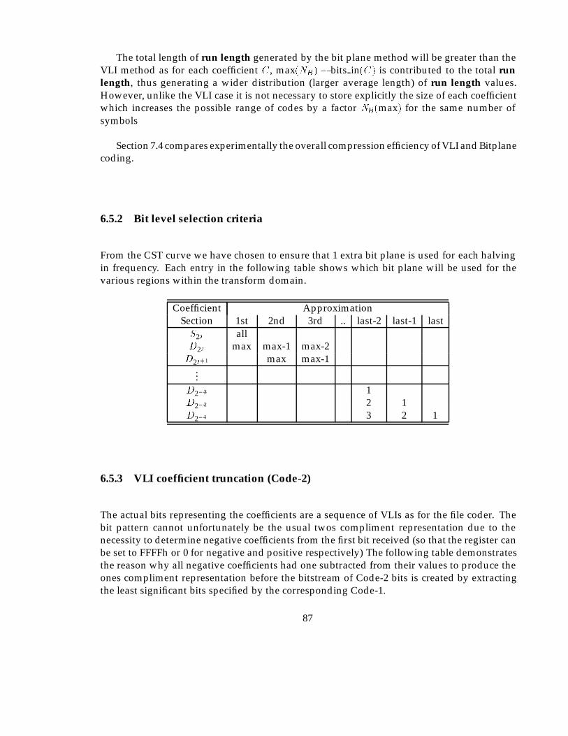
The total length of run length generated by the bit plane method will be greater than theVLI method as for each coefficient C, max(NB) � bits in(C) is contributed to the total runlength, thus generating a wider distribution (larger average length) of run length values.However, unlike the VLI case it is not necessary to store explicitly the size of each coefficientwhich increases the possible range of codes by a factor NB(max) for the same number ofsymbols

Section 7.4 compares experimentally the overall compression efficiency of VLI and Bitplanecoding.

6.5.2 Bit level selection criteria

From the CST curve we have chosen to ensure that 1 extra bit plane is used for each halvingin frequency. Each entry in the following table shows which bit plane will be used for thevarious regions within the transform domain.

Coefficient ApproximationSection 1st 2nd 3rd .. last-2 last-1 lastS2j allD2j max max-1 max-2D2j+1 max max-1

...D2�3 1D2�2 2 1D2�1 3 2 1

6.5.3 VLI coefficient truncation (Code-2)

The actual bits representing the coefficients are a sequence of VLIs as for the file coder. Thebit pattern cannot unfortunately be the usual twos compliment representation due to thenecessity to determine negative coefficients from the first bit received (so that the register canbe set to FFFFh or 0 for negative and positive respectively) The following table demonstratesthe reason why all negative coefficients had one subtracted from their values to produce theones compliment representation before the bitstream of Code-2 bits is created by extractingthe least significant bits specified by the corresponding Code-1.

87

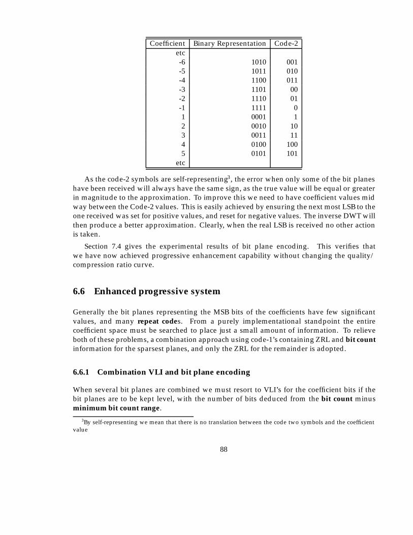
Coefficient Binary Representation Code-2etc-6 1010 001-5 1011 010-4 1100 011-3 1101 00-2 1110 01-1 1111 01 0001 12 0010 103 0011 114 0100 1005 0101 101

etc

As the code-2 symbols are self-representing3, the error when only some of the bit planeshave been received will always have the same sign, as the true value will be equal or greaterin magnitude to the approximation. To improve this we need to have coefficient values midway between the Code-2 values. This is easily achieved by ensuring the next most LSB to theone received was set for positive values, and reset for negative values. The inverse DWT willthen produce a better approximation. Clearly, when the real LSB is received no other actionis taken.

Section 7.4 gives the experimental results of bit plane encoding. This verifies thatwe have now achieved progressive enhancement capability without changing the quality/compression ratio curve.

6.6 Enhanced progressive system

Generally the bit planes representing the MSB bits of the coefficients have few significantvalues, and many repeat codes. From a purely implementational standpoint the entirecoefficient space must be searched to place just a small amount of information. To relieveboth of these problems, a combination approach using code-1’s containing ZRL and bit countinformation for the sparsest planes, and only the ZRL for the remainder is adopted.

6.6.1 Combination VLI and bit plane encoding

When several bit planes are combined we must resort to VLI’s for the coefficient bits if thebit planes are to be kept level, with the number of bits deduced from the bit count minusminimum bit count range.

3By self-representing we mean that there is no translation between the code two symbols and the coefficientvalue

88

6.7 Entropy coding table generation

6.7.1 Statistical distribution

The set of coefficients generated by the chosen transform have interesting statistical propertieswhen applied to natural images, these in turn are passed to the code-1’s due to their closerelationship. It is interesting to note, as several authors previously have done (Mallat,1989) that this is only a feature of the subset of possible datasets in which natural imagesseem to occur, and for an arbitrary dataset may not be the case since the coefficients are adecomposition in an othonormal family and are therefore uncorrelated. Figure 6.8 shows atypical real image and the coefficient distributions associated with it. These have been plottedfor each scale and show a characteristic distribution shape common to most ‘natural’ imageswhich in practice have remarkably similar properties. Essentially, the largest coefficientshave the lowest frequency (probability), with the smaller coefficients having the highestfrequency. This makes entropy encoding an effective final step in reducing the number of bitsrequired to store the image, as a comparison, figure 6.9 shows the distribution for an artificialimage, producing a noticeably less well defined distribution. The two main alternativealgorithms available are Huffman based coding and Arithmetic Coding. The implementationuses Huffman coding due to the lower memory and processing requirements. Huffmancoding only gives optimum (theoretical entropy) encoding when the source symbols have aprobability of 1=2n for integer n. This is rarely the case and therefore arithmetic coding willgive better compression ratios as it can adapt to any distribution.

The next consideration is the number of distributions to use. It is clear from figure 6.9 thata characteristic distribution is formed at each scale of the transform; the coefficients from eachdirectional component on the same scale having approximately similar distributions, withdifferent scales producing different distributions (as well as different numbers of coefficients).We adopt the strategy of providing separate tables for the statistical coding of coefficients ateach scale. For VLI encoding, only this number of statistical models is required, i.e. one foreach scale. When we consider progressive selection of coefficients on a bit plane basis, where itis a set of run lengths which provide the symbols to be coded, each bit-plane also has differentdistribution of run lengths requiring more tables. A maximum of number scales�NB(max)tables might be used, although it is very likely that some will be empty.

6.7.2 Application of tables

Huffman encoding is performed by generating a set of unequal length codes allowing shortcodes to be used for symbols with high probability, and longer codes for symbols with lowprobability. The codes are required to have the property that no valid code is contained asthe beginning of another code, the codes thus require no separator as the end of each (andhence the beginning of the next) is uniquely defined. In this case the codes will be a sequenceof variable length bit patterns.

Two versions of Huffman coding are available. The simplest requires the statisticaldistribution of the symbols to be known in advance, from which a table of code bits is

89

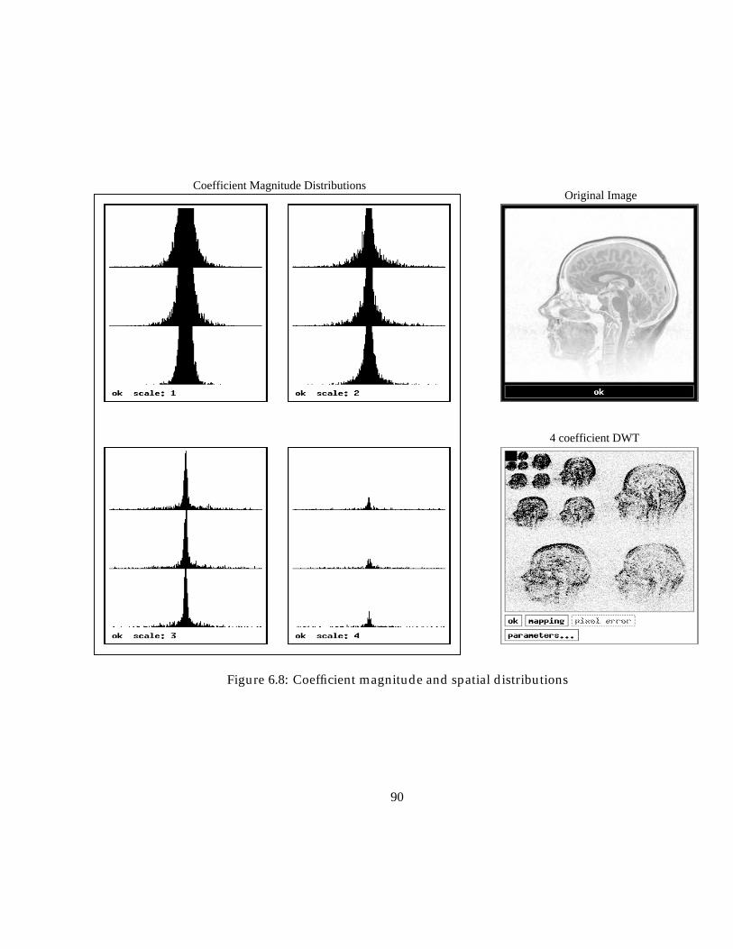
4 coefficient DWT

Original ImageCoefficient Magnitude Distributions

Figure 6.8: Coefficient magnitude and spatial distributions

90

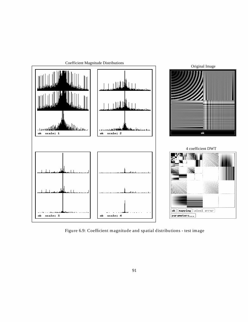
4 coefficient DWT

Original ImageCoefficient Magnitude Distributions

Figure 6.9: Coefficient magnitude and spatial distributions - test image

91

generated via the generation of a binary tree structure. The encoder finds the code bits foreach symbol by simply referencing the look up table. The decoder will traverse the treefrom the root, for each symbol, and follow the branch at each node according to the next bitreceived, until a leaf node is reached when the appropriate original symbol can be determined.Clearly the table, or tree (one can be generated from the other) must also be available to bothencoder and decoder. If the table is not known at the decoder this must be considered whendetermining the efficiency of this scheme.

The alternative version known as Adaptive Huffman coding, refer to Apiki (Apiki, 1991)for an overview, allows the tree to be constructed as decoding takes place. As this addsa number of complications and is not as efficient - in as much as its capability to adapt tochanging symbol statistics is not required - and was not used for our initial experiments asmore advanced arithmetic encoders could be used. We also discovered that the distribution ofthe symbols could be modelled relatively well by a simple function, eliminating the necessityto transmit the encoding tables, as they can be reconstructed with 3 coefficients.

6.7.3 Encoding sets of tables

Previously, we mentioned that empirical analysis of the histogram for each scale and ori-entation of coefficients for a number of images reveals a set of characteristically shapeddistributions. If we assume the distributions derived from these are to be used for theHuffman coding, a number of approaches are possible:

� Include the data required to store the tables along with the symbol data.

� Set up standard tables for each type of image.

� Generate tables from a model, with a small number of parameters.

Including the tables in the coded data will reduce coding efficiency, especially as several arerequired (one for each scale) although there is an advantage for file compression in that nonappearing symbols are disregarded, thus shortening codes for low probability symbols. If ROIselection is required the exact set of symbols cannot be determined in advance, because thescanning sequence is likely to change, thus changing the actual run length codes generated(although not significantly the statistics of the distribution). This implies a code must be madeavailable for every possible symbol and the advantage is thus lost.

Creating a set of tables which can be stored by receiver and transmitter and allows selectionbased on image type, or best match from available tables could be attractive if the match issufficiently good so as not to degrade performance. The space required to store these alongwith the possibility of incorrect assumptions by the encoder concerning the availability ofparticular tables could cause problems.

The final option considered here has potential to be the most useful if it is true that asufficiently good model can be made, such that the loss of efficiency by doing this is less thanwould have been achieved by the first option.

92

6.7.4 Modelling of tables

This section will determine how effectively we can model the statistics of the symbolsproduced by the encoder. Once this has been achieved we are not limited to using onlya few sets of encoding tables, as the storage space allocated to the table becomes far less ofa contributing factor. It is therefore possible to match the run length statistics for each scaleand bit plane.

The distributions appear to be of exponential form,

P (x) � Ke�(jxj=�)�

leaving us the objective of findng the values of �, �, and K which give the best fit (minimumerror) to the actual probabilities. For our purposes P (x) will represent the number ofoccurrences of each symbol (run length) rather than the actual coefficient probability. Asthis function is used to build variable length codes small errors in the predictor function havelittle or no effect on the overall encoding efficiency. This is particularly true when Huffmancoding is used, as it is suboptimal for most distributions in practice. As it proved difficult toanalyse P (x) analytically a combination of numerical techniques was used. This is performedin two stages:

� Stage 1 finds K based on the most frequently occurring symbol.

� Stage 2 estimates �, the variances of the distribution.

� Stage 3 finds the value of � which minimises the error of the predictor function.

6.7.4.1 Finding K

The constantK represents the number of occurrences of the zero coefficient in the model. Theactual measured value of the number of zero coefficients can be used for K, although obviouslyit is possible that this is not the optimal value for fitment of the rest of the distribution, but inpractice there does not appear to be any problem.

6.7.4.2 Estimating �

At the point where P (x) = K=e, the value of P (x) does not depend upon �, and so by findingan approximation to x where the sampled number of symbols is approximately K=e a valueof � can be found.

In practice of course we have a discrete number of samples on the ‘curve’ as well as errors.To over come this � is estimated by linear interpolation between the points P (a) and P (b). IfM is the largest valid symbol index, and given a; b; x 2 N+ we ensure that a and b satisfy thefollowing:

(a; x < M)

�(P (a+ 1) <

k

e) ^ (8x � a)((P (x) >

k

e) _ (P (x) = 0))

�;

93

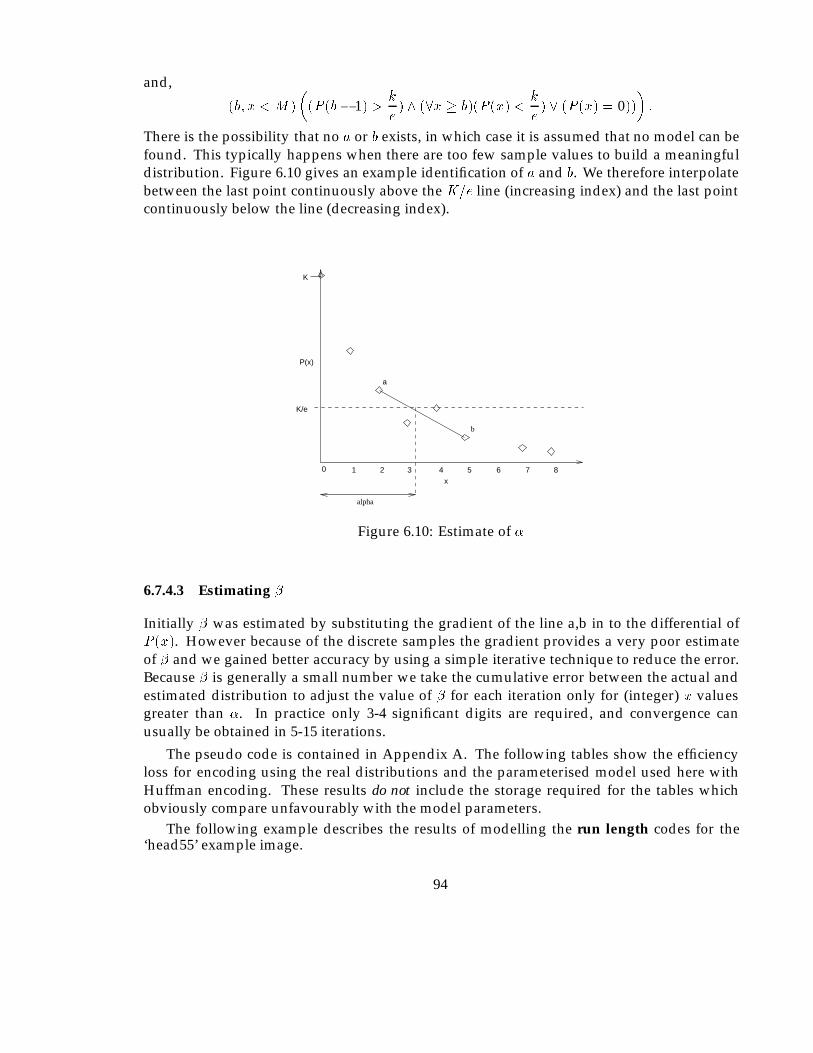
and,

(b; x < M)

�(P (b� 1) >

k

e) ^ (8x � b)(P (x) <

k

e) _ (P (x) = 0))

�:

There is the possibility that no a or b exists, in which case it is assumed that no model can befound. This typically happens when there are too few sample values to build a meaningfuldistribution. Figure 6.10 gives an example identification of a and b. We therefore interpolatebetween the last point continuously above the K=e line (increasing index) and the last pointcontinuously below the line (decreasing index).

K

alpha

2 3 4 5 6 7 8

b

a

0

P(x)

x1

K/e

Figure 6.10: Estimate of �

6.7.4.3 Estimating �

Initially � was estimated by substituting the gradient of the line a,b in to the differential ofP (x). However because of the discrete samples the gradient provides a very poor estimateof � and we gained better accuracy by using a simple iterative technique to reduce the error.Because � is generally a small number we take the cumulative error between the actual andestimated distribution to adjust the value of � for each iteration only for (integer) x valuesgreater than �. In practice only 3-4 significant digits are required, and convergence canusually be obtained in 5-15 iterations.

The pseudo code is contained in Appendix A. The following tables show the efficiencyloss for encoding using the real distributions and the parameterised model used here withHuffman encoding. These results do not include the storage required for the tables whichobviously compare unfavourably with the model parameters.

The following example describes the results of modelling the run length codes for the‘head55’ example image.

94

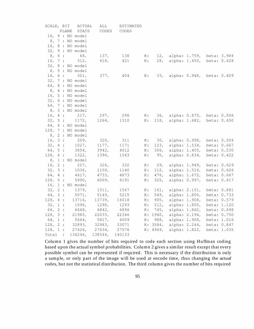
SCALE, BIT ACTUAL ALL ESTIMATEDPLANE STATS CODES CODES

16, 9 : NO model8, 7 : NO model16, 8 : NO model32, 9 : NO model8, 6 : 64, 137, 138 K: 12, alpha: 1.759, beta: 3.98416, 7 : 312, 418, 421 K: 28, alpha: 1.450, beta: 0.42832, 8 : NO model8, 5 : NO model16, 6 : 301, 377, 404 K: 33, alpha: 0.948, beta: 0.40932, 7 : NO model64, 8 : NO model8, 4 : NO model16, 5 : NO model32, 6 : NO model64, 7 : NO model8, 3 : NO model16, 4 : 217, 297, 296 K: 36, alpha: 0.875, beta: 0.50632, 5 : 1172, 1264, 1310 K: 118, alpha: 1.682, beta: 0.65064, 6 : NO model128, 7 : NO model8, 2 : NO model16, 3 : 209, 320, 311 K: 30, alpha: 0.998, beta: 0.50432, 4 : 1027, 1177, 1171 K: 123, alpha: 1.534, beta: 0.66764, 5 : 3854, 3942, 4012 K: 306, alpha: 1.405, beta: 0.530128, 6 : 1322, 1396, 1563 K: 95, alpha: 0.834, beta: 0.4228, 1 : NO model16, 2 : 227, 326, 332 K: 29, alpha: 1.949, beta: 0.62932, 3 : 1036, 1150, 1140 K: 112, alpha: 1.516, beta: 0.62664, 4 : 4617, 4733, 4873 K: 476, alpha: 1.672, beta: 0.667128, 5 : 5990, 6009, 6191 K: 325, alpha: 0.997, beta: 0.41716, 1 : NO model32, 2 : 1379, 1511, 1547 K: 161, alpha: 2.151, beta: 0.88164, 3 : 5071, 5149, 5215 K: 549, alpha: 1.800, beta: 0.733128, 4 : 13716, 13739, 14018 K: 905, alpha: 1.908, beta: 0.57932, 1 : 1096, 1290, 1293 K: 212, alpha: 1.805, beta: 1.12064, 2 : 6668, 6842, 6896 K: 745, alpha: 1.862, beta: 0.698128, 3 : 21985, 22033, 22346 K: 1940, alpha: 2.194, beta: 0.75064, 1 : 5664, 5817, 6009 K: 988, alpha: 1.908, beta: 1.016128, 2 : 32893, 32983, 33071 K: 3584, alpha: 2.244, beta: 0.847128, 1 : 27426, 27634, 27576 K: 4949, alpha: 1.822, beta: 1.035Total : 136246, 138544, 140133

Column 1 gives the number of bits required to code each section using Huffman codingbased upon the actual symbol probabilities. Column 2 gives a similar result except that everypossible symbol can be represented if required. This is necessary if the distribution is onlya sample, or only part of the image will be used at encode time, thus changing the actualcodes, but not the statistical distribution. The third column gives the number of bits required

95

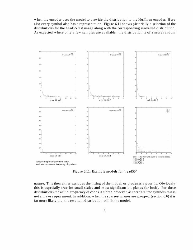
when the encoder uses the model to provide the distribution to the Huffman encoder. Herealso every symbol also has a representation. Figure 6.11 shows pictorially a selection of thedistributions for the head55 test image along with the corresponding modelled distribution.As expected where only a few samples are available. the distribution is of a more random

0

5

10

15

20

25

30

35

40

0 20 40 60 80 100 120 140

"32-8""32-7""16-5"

0

500

1000

1500

2000

2500

3000

3500

4000

4500

5000

0 20 40 60 80 100 120 140

"128-1"4949*exp(-(abs(x)/1.822)**1.035)

0

50

100

150

200

250

300

350

0 20 40 60 80 100 120 140

"64-5"306*exp(-(abs(x)/1.405)**0.530)

0

50

100

150

200

250

300

350

0 20 40 60 80 100 120 140

"128-5"325*exp(-(abs(x)/0.997)**0.417)

0

100

200

300

400

500

600

700

800

0 20 40 60 80 100 120 140

"64-2"745*exp(-(abs(x)/1.862)**0.698)

0

100

200

300

400

500

600

700

800

900

1000

0 20 40 60 80 100 120 140

"64-1"988*exp(-(abs(x)/1.908)**1.016)

abscissa represents symbol indexordinate represents frequency of symbols

scale 64, bit 5 scale 128, bit 5 scale 64, bit 2

scale 128, bit 1scale 64, bit 1 Three datasets which failed to produce models scale 32, bit 8scale 32, bit 7scale 16, bit 5

Figure 6.11: Example models for ‘head55’

nature. This then either excludes the fitting of the model, or produces a poor fit. Obviouslythis is especially true for small scales and most significant bit planes (or both). For thesedistributions the actual frequency of codes is stored however, as there are few symbols this isnot a major requirement. In addition, when the sparsest planes are grouped (section 6.6) it isfar more likely that the resultant distribution will fit the model.

96

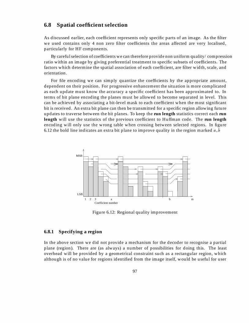
6.8 Spatial coefficient selection

As discussed earlier, each coefficient represents only specific parts of an image. As the filterwe used contains only 4 non zero filter coefficients the areas affected are very localised,particularly for HF components.

By careful selection of coefficients we can therefore provide non uniform quality/compressionratio within an image by giving preferential treatment to specific subsets of coefficients. Thefactors which determine the spatial association of each coefficient, are filter width, scale, andorientation.

For file encoding we can simply quantize the coefficients by the appropriate amount,dependent on their position. For progressive enhancement the situation is more complicatedas each update must know the accuracy a specific coefficient has been approximated to. Interms of bit plane encoding the planes must be allowed to become separated in level. Thiscan be achieved by associating a bit-level mask to each coefficient when the most significantbit is received. An extra bit plane can then be transmitted for a specific region allowing futureupdates to traverse between the bit planes. To keep the run length statistics correct each runlength will use the statistics of the previous coefficient to Huffman code. The run lengthencoding will only use the wrong table when crossing between selected regions. In figure6.12 the bold line indicates an extra bit plane to improve quality in the region marked a; b

Coefficient number1 2 3

LSB

MSB

ma b

Figure 6.12: Regional quality improvement

6.8.1 Specifying a region

In the above section we did not provide a mechanism for the decoder to recognise a partialplane (region). There are (as always) a number of possibilities for doing this. The leastoverhead will be provided by a geometrical constraint such as a rectangular region, whichalthough is of no value for regions identified from the image itself, would be useful for user

97

selections in a progressive enhancement situation. Slightly more complex regions could bespecified by a series of points on an irregular polygon, as long as exactly the same coefficientsfall inside and outside the area. For large areas all unwanted coefficients could be neglectedusing ZRL codes, allowing an entirely arbitrary area to be enhanced. The overhead in ZRLrepeat symbols could become high however if the area is small.

There are more complex possibilities, which have been considered, for instance for regionswith convex only edges, the position of the first required coefficient, followed by an offset foreach new scan might be possible, giving a reasonably low overhead, combined with flexibleselection of regions.

6.8.2 Background removal

The background of many images typically contains a lot of random noise. This is the part ofthe signal which is removed first by lossy compression algorithms. For high ratio compressionwe would not therefore expect any significant improvement in compression efficiency. Thereal benefit would be expected to be at the lower ratios when this random noise is startingto be reproduced. The gain will be maximised when the image becomes indistinguishablefrom the original, at a higher overall compression ratio than it would have otherwise. Sometypes of image respond to very simple techniques for instance the ‘head55’ image can beseparated from the background by simply thresholding the detail wavelet coefficients. Thethreshold can be calculated from the edge regions for this type of image as it is known thatthe extremities of this class (i.e. CT headscan) of image are background.

6.9 Manipulation of the coded image

For some basic image processing operations it is more efficient to process the image in itsDWT function space, and should be possible on images regardless of the compression ratio.

Some possible operations are listed, indicating at which stage, and of what nature theprocessing would take. Further investigation of this aspect has not taken place, but it willshare some similarities with similar DCT operations discussed in (Smith & Rowe, 1993) in thecontext of JPEG. The operations considered are:

Scalar multiplication. The visual effect of this operation is to increase the dynamic range ofan image. This operation is usefully applied to faint images, or those where we wishto extract detail from an area of similar intensity. This operation will be performed byscaling the wavelet coefficients by the appropriate factor.

Scalar addition. Adding a constant value to all pixels within an image will brighten it(positive constant) or make it dimmer (negative constant). To achieve this we onlyrequire to add the appropriate value to the lowest resolution or average image.

98

Pixel addition. The ability to add two images could prove useful for annotation or markingof images, as well as the superposition of two images or taking the difference of twoimages (e.g. DSA), addition of the coefficients will achieve this.

6.10 Summary of encoding strategy

In the previous sections, a number of ideas have been brought together to allow an en-coded stream of bits to be generated from the transformed image data. The process ofbit plane encoding produces a fairly fine grained progressive enhancement capability, andexperiments with contrast masking which require a non uniform quantizer produce slightlybetter reproduction at high compression ratios. Figure 6.13 shows the stages involved in thequantizing and encoding process. The dashed line on this diagram indicates a path whichhas not been implemented but should provide the best result of all given the restrictionsdiscussed previously in section 6.3.1.

99

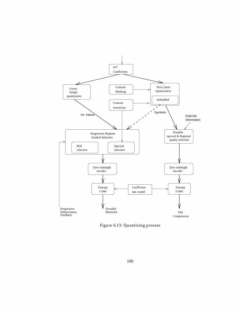
WT

Coefficients

Contrast

Masking

Contrast

Sensitivity

encoderZero runlength

encoderZero runlength

Int. Values

selection

Progressive Bitplane

Quantization

embeddedquantization

ROIselectionSpectral

Symbol Selection spectral & Regionalquality selection

Possible

Non Linear

IntegerLinear

CoderEntropy

FileCompression

EntropyCoder

ExternalInformation

Symbols

BitstreamEncoded

EnhancementProgressive

Feedback

Coefficient

stat. model

Figure 6.13: Quantizing process

100

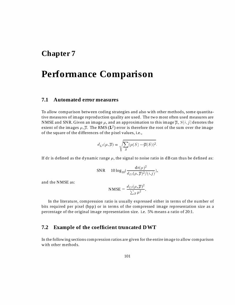
Chapter 7

Performance Comparison

7.1 Automated error measures

To allow comparison between coding strategies and also with other methods, some quantita-tive measures of image reproduction quality are used. The two most often used measures areNMSE and SNR. Given an image �, and an approximation to this image �, S(i; j)denotes theextent of the images �; �. The RMS (L2) error is therefore the root of the sum over the imageof the square of the differences of the pixel values, i.e.,

dL2(�; �) =

sXS

(�(S)� �(S))2:

If dr is defined as the dynamic range �, the signal to noise ratio in dB can thus be defined as:

SNR = 10 log10(dr(�)2

dL2(�; �)2=(i:j));

and the NMSE as:

NMSE =dL2(�; �)2P

S�2 :

In the literature, compression ratio is usually expressed either in terms of the number ofbits required per pixel (bpp) or in terms of the compressed image representation size as apercentage of the original image representation size. i.e. 5% means a ratio of 20:1.

7.2 Example of the coefficient truncated DWT

In the following sections compression ratios are given for the entire image to allow comparisonwith other methods.

101

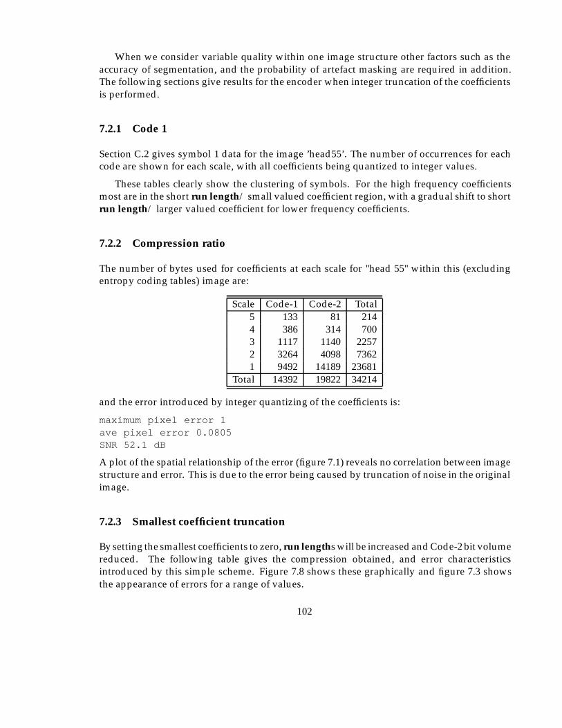
When we consider variable quality within one image structure other factors such as theaccuracy of segmentation, and the probability of artefact masking are required in addition.The following sections give results for the encoder when integer truncation of the coefficientsis performed.

7.2.1 Code 1

Section C.2 gives symbol 1 data for the image ’head55’. The number of occurrences for eachcode are shown for each scale, with all coefficients being quantized to integer values.

These tables clearly show the clustering of symbols. For the high frequency coefficientsmost are in the short run length/ small valued coefficient region, with a gradual shift to shortrun length/ larger valued coefficient for lower frequency coefficients.

7.2.2 Compression ratio

The number of bytes used for coefficients at each scale for "head 55" within this (excludingentropy coding tables) image are:

Scale Code-1 Code-2 Total5 133 81 2144 386 314 7003 1117 1140 22572 3264 4098 73621 9492 14189 23681

Total 14392 19822 34214

and the error introduced by integer quantizing of the coefficients is:

maximum pixel error 1ave pixel error 0.0805SNR 52.1 dB

A plot of the spatial relationship of the error (figure 7.1) reveals no correlation between imagestructure and error. This is due to the error being caused by truncation of noise in the originalimage.

7.2.3 Smallest coefficient truncation

By setting the smallest coefficients to zero, run lengths will be increased and Code-2 bit volumereduced. The following table gives the compression obtained, and error characteristicsintroduced by this simple scheme. Figure 7.8 shows these graphically and figure 7.3 showsthe appearance of errors for a range of values.

102

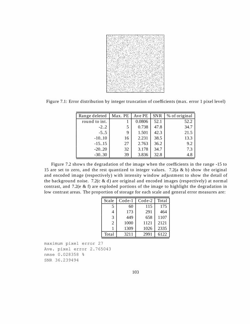
Figure 7.1: Error distribution by integer truncation of coefficients (max. error 1 pixel level)

Range deleted Max. PE Ave PE SNR % of originalround to int. 1 0.0806 52.1 52.2

-2..2 5 0.738 47.8 34.7-5..5 9 1.501 42.3 21.5

-10..10 16 2.231 38.5 13.3-15..15 27 2.763 36.2 9.2-20..20 32 3.178 34.7 7.3-30..30 39 3.836 32.8 4.8

Figure 7.2 shows the degradation of the image when the coefficients in the range -15 to15 are set to zero, and the rest quantized to integer values. 7.2(a & b) show the originaland encoded image (respectively) with intensity window adjustment to show the detail ofthe background noise. 7.2(c & d) are original and encoded images (respectively) at normalcontrast, and 7.2(e & f) are exploded portions of the image to highlight the degradation inlow contrast areas. The proportion of storage for each scale and general error measures are:

Scale Code-1 Code-2 Total5 60 115 1754 173 291 4643 449 658 11072 1000 1121 21211 1309 1026 2335

Total 3211 2991 6122

maximum pixel error 27Ave. pixel error 2.765043nmse 0.028358 %SNR 36.239494

103

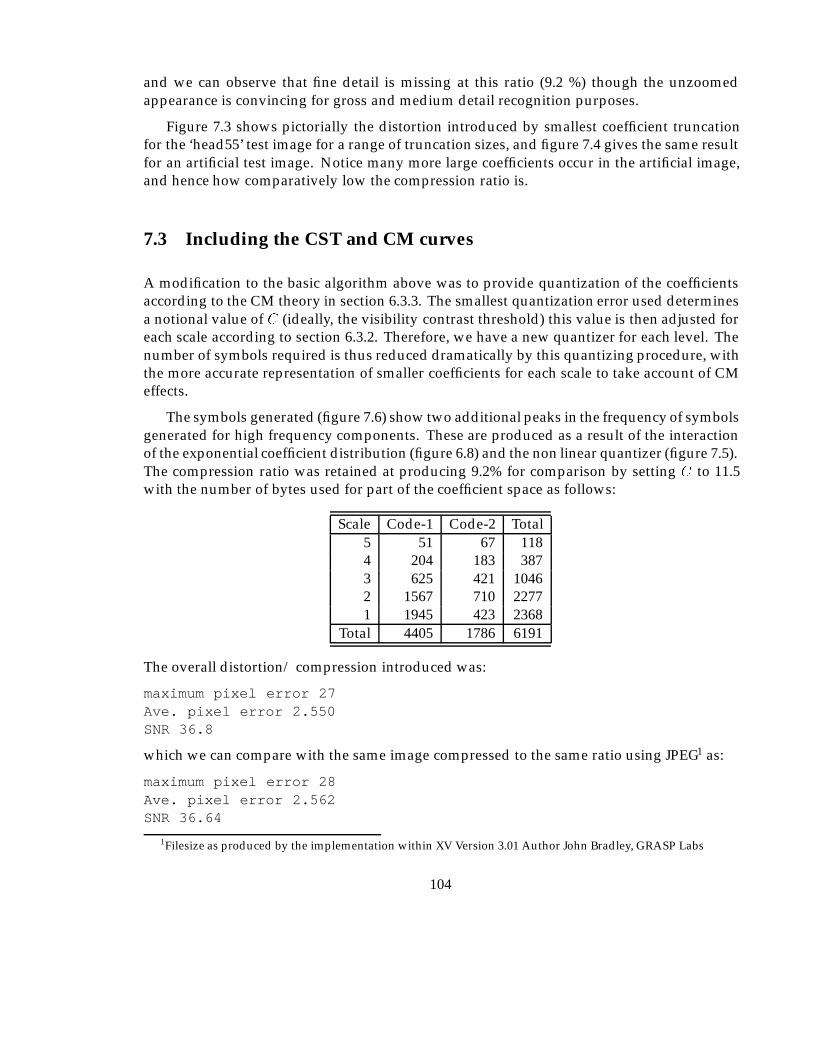
and we can observe that fine detail is missing at this ratio (9.2 %) though the unzoomedappearance is convincing for gross and medium detail recognition purposes.

Figure 7.3 shows pictorially the distortion introduced by smallest coefficient truncationfor the ‘head55’ test image for a range of truncation sizes, and figure 7.4 gives the same resultfor an artificial test image. Notice many more large coefficients occur in the artificial image,and hence how comparatively low the compression ratio is.

7.3 Including the CST and CM curves

A modification to the basic algorithm above was to provide quantization of the coefficientsaccording to the CM theory in section 6.3.3. The smallest quantization error used determinesa notional value of C (ideally, the visibility contrast threshold) this value is then adjusted foreach scale according to section 6.3.2. Therefore, we have a new quantizer for each level. Thenumber of symbols required is thus reduced dramatically by this quantizing procedure, withthe more accurate representation of smaller coefficients for each scale to take account of CMeffects.

The symbols generated (figure 7.6) show two additional peaks in the frequency of symbolsgenerated for high frequency components. These are produced as a result of the interactionof the exponential coefficient distribution (figure 6.8) and the non linear quantizer (figure 7.5).The compression ratio was retained at producing 9.2% for comparison by setting C to 11.5with the number of bytes used for part of the coefficient space as follows:

Scale Code-1 Code-2 Total5 51 67 1184 204 183 3873 625 421 10462 1567 710 22771 1945 423 2368

Total 4405 1786 6191

The overall distortion/ compression introduced was:

maximum pixel error 27Ave. pixel error 2.550SNR 36.8

which we can compare with the same image compressed to the same ratio using JPEG1 as:

maximum pixel error 28Ave. pixel error 2.562SNR 36.64

1Filesize as produced by the implementation within XV Version 3.01 Author John Bradley, GRASP Labs

104

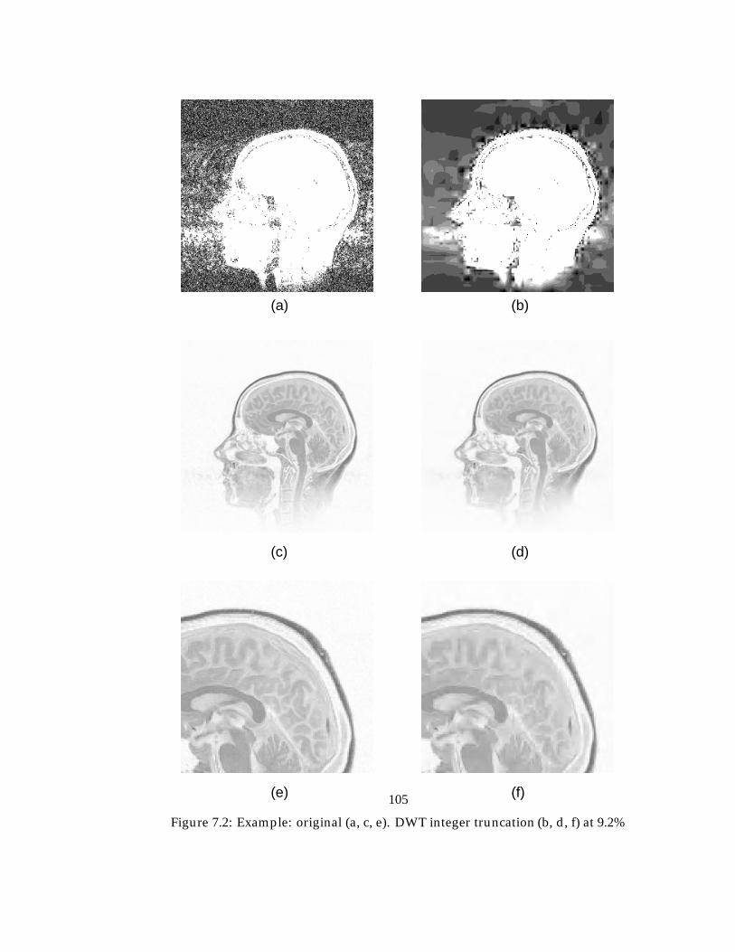
(a)

(e) (f)

(b)

(c) (d)

Figure 7.2: Example: original (a, c, e). DWT integer truncation (b, d, f) at 9.2%

105

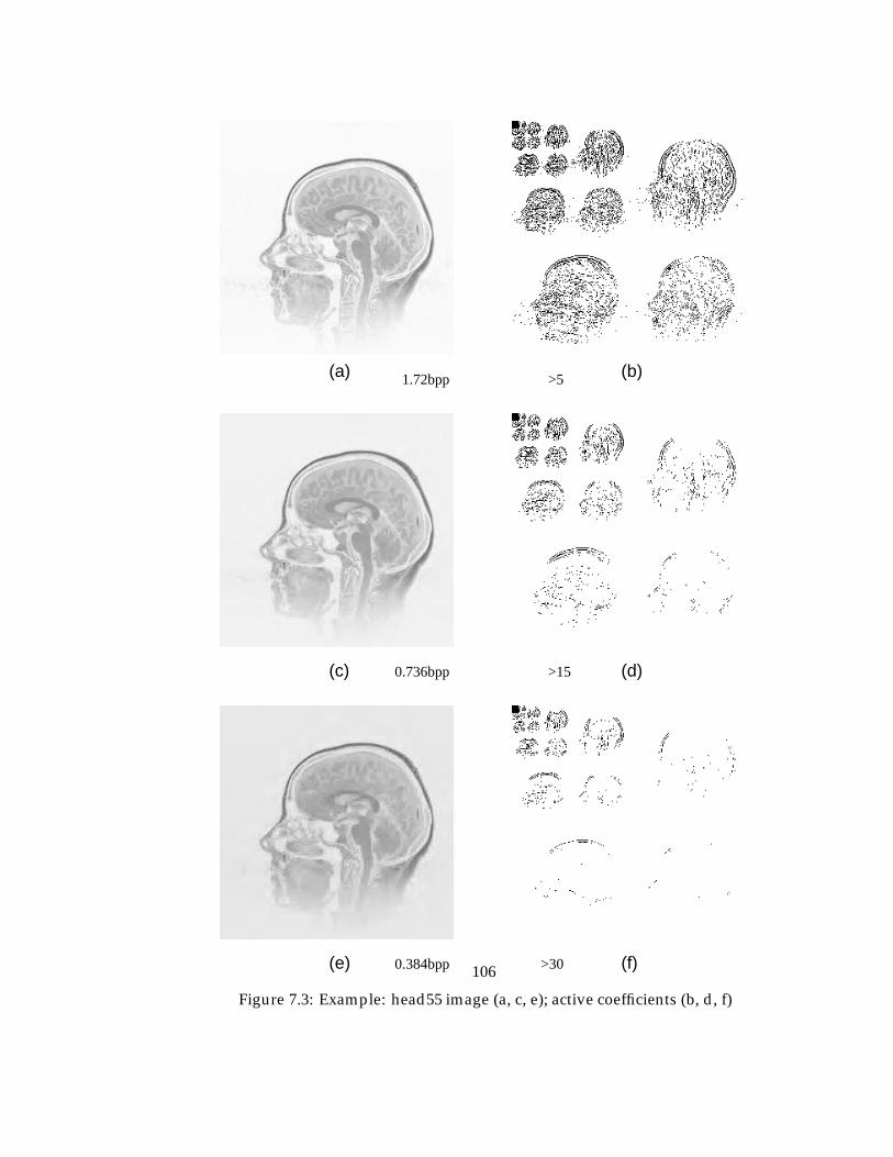
(a)

(e) (f)

(b)

(c) (d)

>30

>15

>51.72bpp

0.736bpp

0.384bpp

Figure 7.3: Example: head55 image (a, c, e); active coefficients (b, d, f)

106

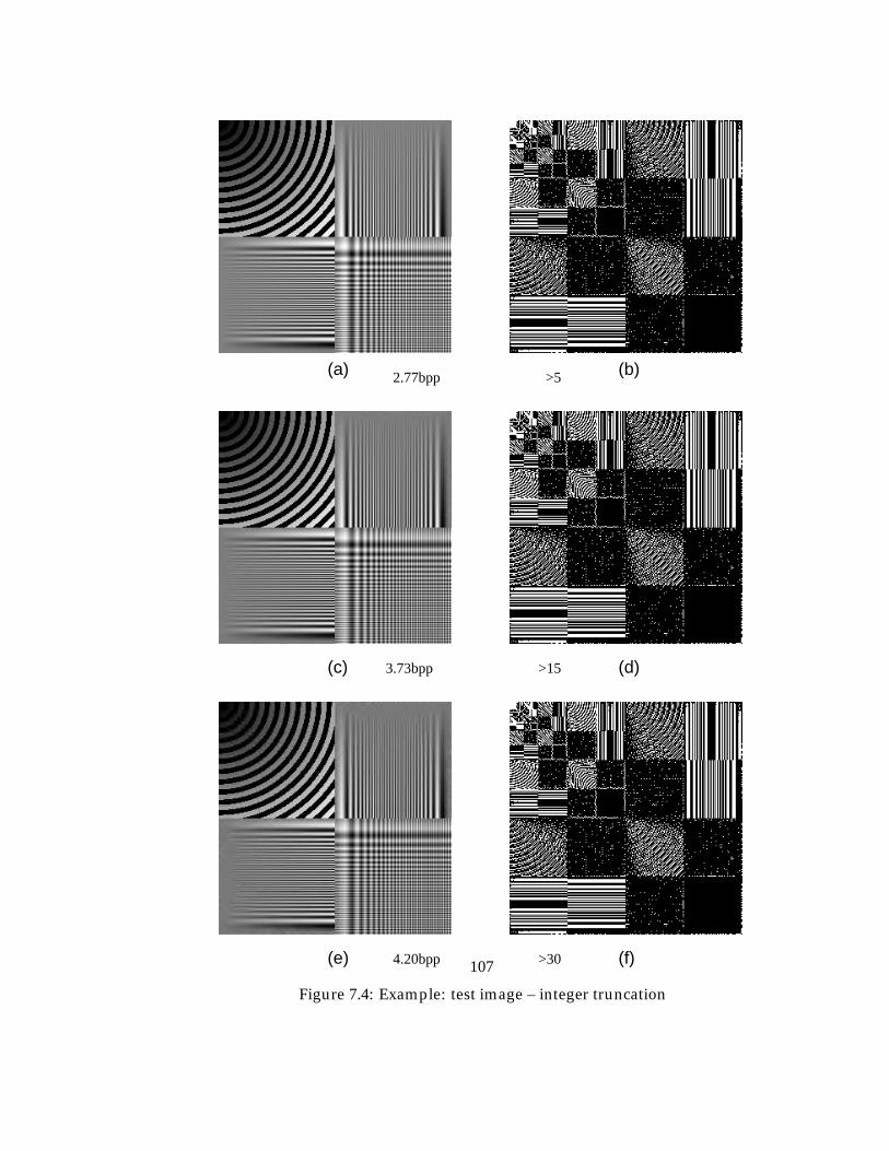
(a)

(e) (f)

(b)

(c) (d)

4.20bpp

3.73bpp

2.77bpp >5

>15

>30

Figure 7.4: Example: test image – integer truncation

107

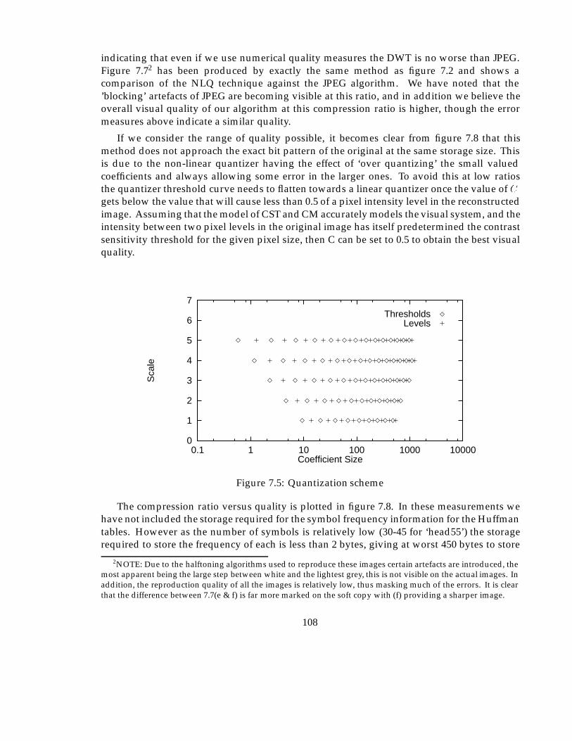
indicating that even if we use numerical quality measures the DWT is no worse than JPEG.Figure 7.72 has been produced by exactly the same method as figure 7.2 and shows acomparison of the NLQ technique against the JPEG algorithm. We have noted that the’blocking’ artefacts of JPEG are becoming visible at this ratio, and in addition we believe theoverall visual quality of our algorithm at this compression ratio is higher, though the errormeasures above indicate a similar quality.

If we consider the range of quality possible, it becomes clear from figure 7.8 that thismethod does not approach the exact bit pattern of the original at the same storage size. Thisis due to the non-linear quantizer having the effect of ‘over quantizing’ the small valuedcoefficients and always allowing some error in the larger ones. To avoid this at low ratiosthe quantizer threshold curve needs to flatten towards a linear quantizer once the value of Cgets below the value that will cause less than 0.5 of a pixel intensity level in the reconstructedimage. Assuming that the model of CST and CM accurately models the visual system, and theintensity between two pixel levels in the original image has itself predetermined the contrastsensitivity threshold for the given pixel size, then C can be set to 0.5 to obtain the best visualquality.

0

1

2

3

4

5

6

7

0.1 1 10 100 1000 10000

Sca

le

Coefficient Size

ThresholdsLevels

Figure 7.5: Quantization scheme

The compression ratio versus quality is plotted in figure 7.8. In these measurements wehave not included the storage required for the symbol frequency information for the Huffmantables. However as the number of symbols is relatively low (30-45 for ‘head55’) the storagerequired to store the frequency of each is less than 2 bytes, giving at worst 450 bytes to store

2NOTE: Due to the halftoning algorithms used to reproduce these images certain artefacts are introduced, themost apparent being the large step between white and the lightest grey, this is not visible on the actual images. Inaddition, the reproduction quality of all the images is relatively low, thus masking much of the errors. It is clearthat the difference between 7.7(e & f) is far more marked on the soft copy with (f) providing a sharper image.

108

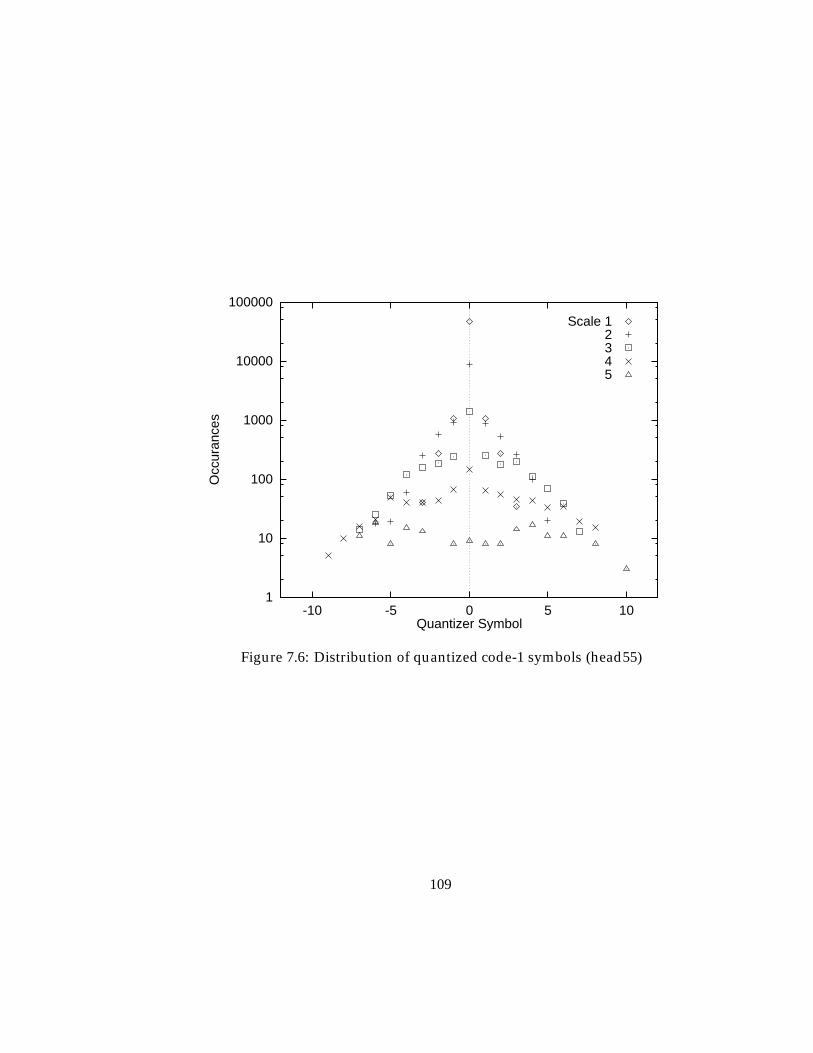
1

10

100

1000

10000

100000

-10 -5 0 5 10

Occ

uran

ces

Quantizer Symbol

Scale 12345

Figure 7.6: Distribution of quantized code-1 symbols (head55)

109

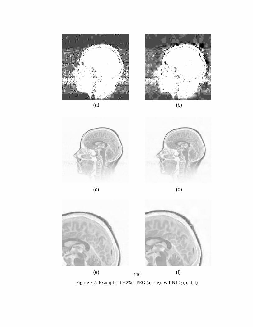
(a)

(e) (f)

(b)

(c) (d)

Figure 7.7: Example at 9.2%: JPEG (a, c, e). WT NLQ (b, d, f)

110

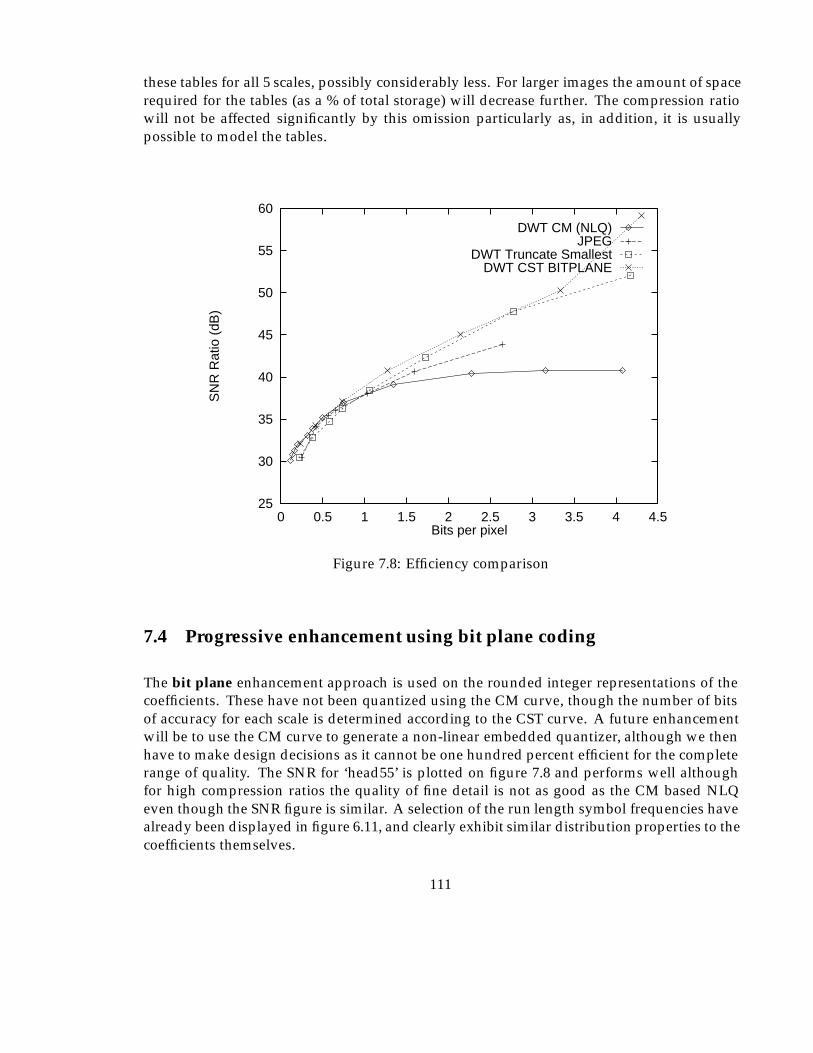
these tables for all 5 scales, possibly considerably less. For larger images the amount of spacerequired for the tables (as a % of total storage) will decrease further. The compression ratiowill not be affected significantly by this omission particularly as, in addition, it is usuallypossible to model the tables.

25

30

35

40

45

50

55

60

0 0.5 1 1.5 2 2.5 3 3.5 4 4.5

SN

R R

atio

(dB

)

Bits per pixel

DWT CM (NLQ)JPEG

DWT Truncate SmallestDWT CST BITPLANE

Figure 7.8: Efficiency comparison

7.4 Progressive enhancement using bit plane coding

The bit plane enhancement approach is used on the rounded integer representations of thecoefficients. These have not been quantized using the CM curve, though the number of bitsof accuracy for each scale is determined according to the CST curve. A future enhancementwill be to use the CM curve to generate a non-linear embedded quantizer, although we thenhave to make design decisions as it cannot be one hundred percent efficient for the completerange of quality. The SNR for ‘head55’ is plotted on figure 7.8 and performs well althoughfor high compression ratios the quality of fine detail is not as good as the CM based NLQeven though the SNR figure is similar. A selection of the run length symbol frequencies havealready been displayed in figure 6.11, and clearly exhibit similar distribution properties to thecoefficients themselves.

111

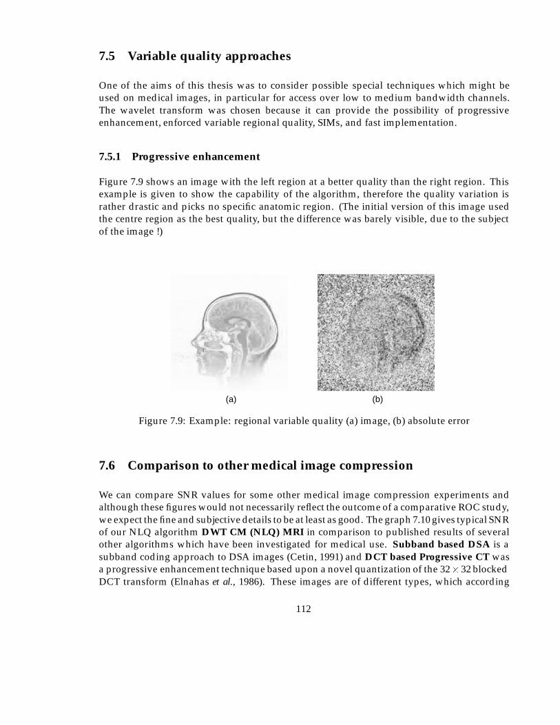
7.5 Variable quality approaches

One of the aims of this thesis was to consider possible special techniques which might beused on medical images, in particular for access over low to medium bandwidth channels.The wavelet transform was chosen because it can provide the possibility of progressiveenhancement, enforced variable regional quality, SIMs, and fast implementation.

7.5.1 Progressive enhancement

Figure 7.9 shows an image with the left region at a better quality than the right region. Thisexample is given to show the capability of the algorithm, therefore the quality variation israther drastic and picks no specific anatomic region. (The initial version of this image usedthe centre region as the best quality, but the difference was barely visible, due to the subjectof the image !)

(a) (b)

Figure 7.9: Example: regional variable quality (a) image, (b) absolute error

7.6 Comparison to other medical image compression

We can compare SNR values for some other medical image compression experiments andalthough these figures would not necessarily reflect the outcome of a comparative ROC study,we expect the fine and subjective details to be at least as good. The graph 7.10 gives typical SNRof our NLQ algorithm DWT CM (NLQ) MRI in comparison to published results of severalother algorithms which have been investigated for medical use. Subband based DSA is asubband coding approach to DSA images (Cetin, 1991) and DCT based Progressive CT wasa progressive enhancement technique based upon a novel quantization of the 32� 32 blockedDCT transform (Elnahas et al., 1986). These images are of different types, which according

112

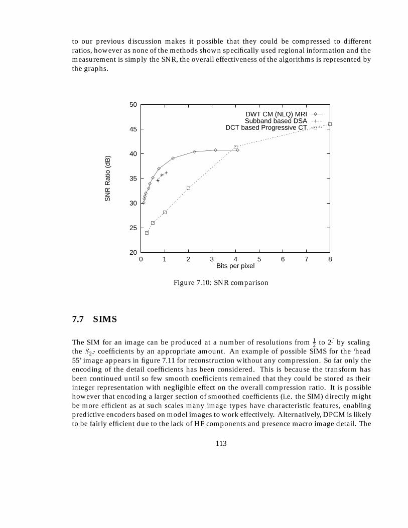
to our previous discussion makes it possible that they could be compressed to differentratios, however as none of the methods shown specifically used regional information and themeasurement is simply the SNR, the overall effectiveness of the algorithms is represented bythe graphs.

20

25

30

35

40

45

50

0 1 2 3 4 5 6 7 8

SN

R R

atio

(dB

)

Bits per pixel

DWT CM (NLQ) MRISubband based DSA

DCT based Progressive CT

Figure 7.10: SNR comparison

7.7 SIMS

The SIM for an image can be produced at a number of resolutions from 12 to 2j by scaling

the S2J coefficients by an appropriate amount. An example of possible SIMS for the ‘head55’ image appears in figure 7.11 for reconstruction without any compression. So far only theencoding of the detail coefficients has been considered. This is because the transform hasbeen continued until so few smooth coefficients remained that they could be stored as theirinteger representation with negligible effect on the overall compression ratio. It is possiblehowever that encoding a larger section of smoothed coefficients (i.e. the SIM) directly mightbe more efficient as at such scales many image types have characteristic features, enablingpredictive encoders based on model images to work effectively. Alternatively, DPCM is likelyto be fairly efficient due to the lack of HF components and presence macro image detail. The

113

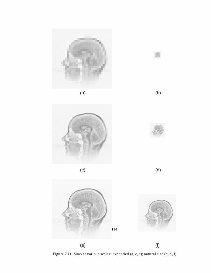
(a)

(e)

(b)

(c) (d)

(f)

Figure 7.11: Sims at various scales: expanded (a, c, e); natural size (b, d, f)

114

table in appendix C.4 gives the 8 � 8 and 16 � 16 smoothed coefficients for ‘head55’, wherethese characteristics can be seen.

115

Chapter 8

Implementation

8.1 Implementation environment

The algorithms described in this work were implemented using the ’C’ programming lan-guage, in a UNIX environment. Although a complete application GUI was not built, the X-Windows protocol and widgets were utilised for the graphical aspects of the experiments, as itis believed that most of the facilities that would be required to create a complete application areavailable. The parts of the encoder/decoder algorithms were implemented as independentprocesses (e.g. decoder, decompressor, interface display) communicating via shared memory.This approach has the advantage that one aspect of the system does not delay the others, inparticular the decompression (IDWT) does not delay the decoder, which can be allowed tooperate at its optimum speed.

8.2 Decoder/encoder implementation

This section describes an overview of the implementation of the encoder and decoderalgorithms. An outline of the major data structures and processing operations for theprogressive codec is given based on the outline algorithms previously described.

Figure 8.1 describes the structures required for implementation of the quantizing and se-lection algorithm in figure 6.13 using bitplane selection and integer quantizing of coefficients.The set of coefficients will have been generated as described in chapter 5.

The components of the encoder/ decoder are as follows:

Transform engine. The transform engine (not shown in figures 8.1) will have produced a setof coefficients with appropriate properties.

Probability tables/Entropy coder tables. Some types of entropy encoding require the prob-ability of each symbol to be known in advance. This is then used to generate a set ofvariable length codes to map the input symbols to an output bit stream.

116

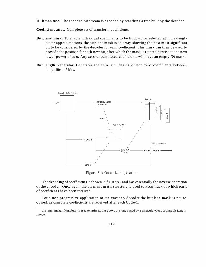
Huffman tree. The encoded bit stream is decoded by searching a tree built by the decoder.

Coefficient array. Complete set of transform coefficients

Bit plane mask. To enable individual coefficients to be built up or selected at increasinglybetter approximations, the bitplane mask is an array showing the next most significantbit to be considered by the decoder for each coefficient. This mask can then be used toprovide the position for each new bit, after which the mask is rotated bitwise to the nextlower power of two. Any zero or completed coefficients will have an empty (0) mask.

Run length Generator. Generates the zero run lengths of non zero coefficients betweeninsignificant1 bits.

Entropy Coder

coded output

-1

scal

e 1

scal

e 2

scal

e 3

generator

len_list

reset

entropy table

s

s -1

-1 s -1

s

send coder tables

Code-1

Code-2

Quantized Coeficients

bit_plane_mask

Figure 8.1: Quantizer operation

The decoding of coefficients is shown in figure 8.2 and has essentially the inverse operationof the encoder. Once again the bit plane mask structure is used to keep track of which partsof coefficients have been received.

For a non-progressive application of the encoder/decoder the bitplane mask is not re-quired, as complete coefficients are received after each Code-1.

1the term ‘insignificant bits’ is used to indicate bits above the range used by a particular Code-2 Variable LengthInteger

117

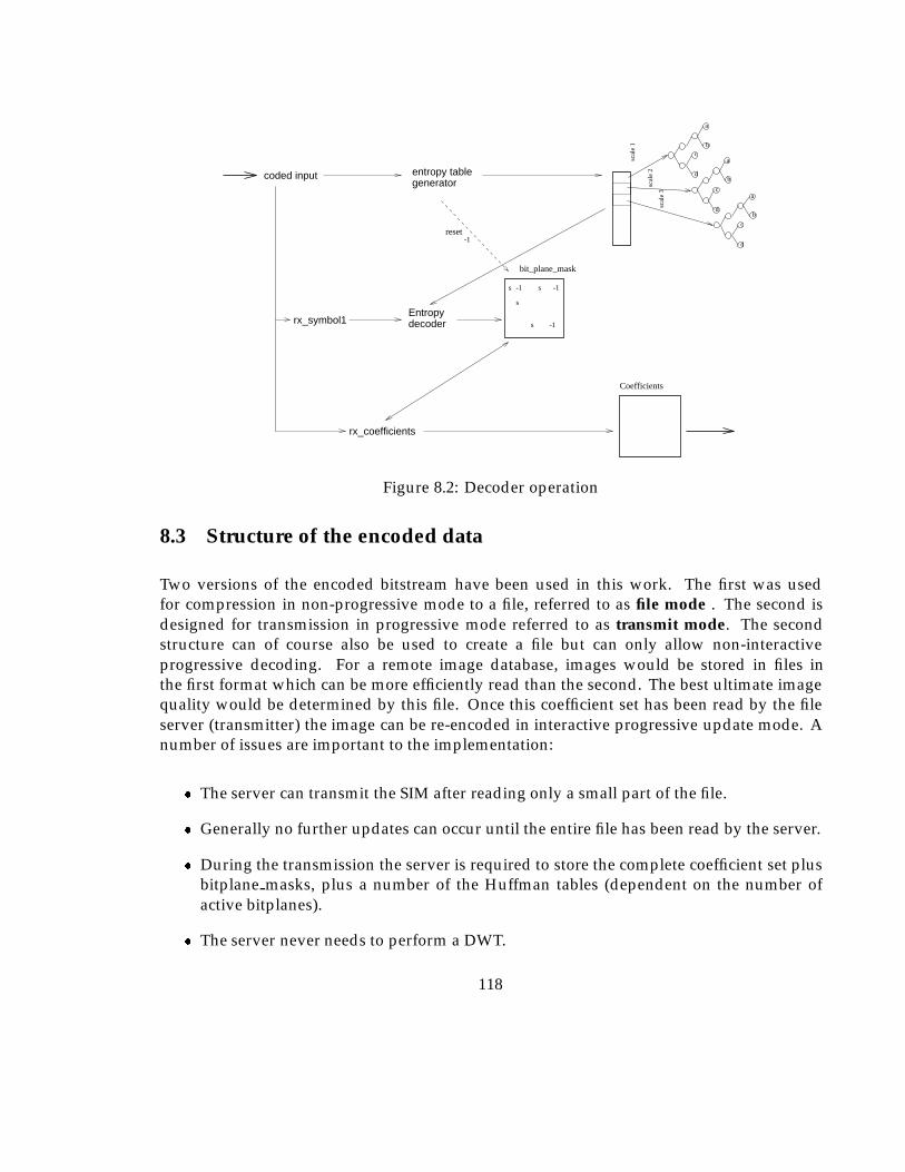
bc

d

a

b

c

d

a

b

c

d

a

Entropy decoder

generatorentropy tablecoded input

scal

e 2

scal

e 1

scal

e 3

reset-1

Coefficients

s

s -1

-1 s -1

s

bit_plane_mask

rx_symbol1

rx_coefficients

Figure 8.2: Decoder operation

8.3 Structure of the encoded data

Two versions of the encoded bitstream have been used in this work. The first was usedfor compression in non-progressive mode to a file, referred to as file mode . The second isdesigned for transmission in progressive mode referred to as transmit mode. The secondstructure can of course also be used to create a file but can only allow non-interactiveprogressive decoding. For a remote image database, images would be stored in files inthe first format which can be more efficiently read than the second. The best ultimate imagequality would be determined by this file. Once this coefficient set has been read by the fileserver (transmitter) the image can be re-encoded in interactive progressive update mode. Anumber of issues are important to the implementation:

� The server can transmit the SIM after reading only a small part of the file.

� Generally no further updates can occur until the entire file has been read by the server.

� During the transmission the server is required to store the complete coefficient set plusbitplane masks, plus a number of the Huffman tables (dependent on the number ofactive bitplanes).

� The server never needs to perform a DWT.

118

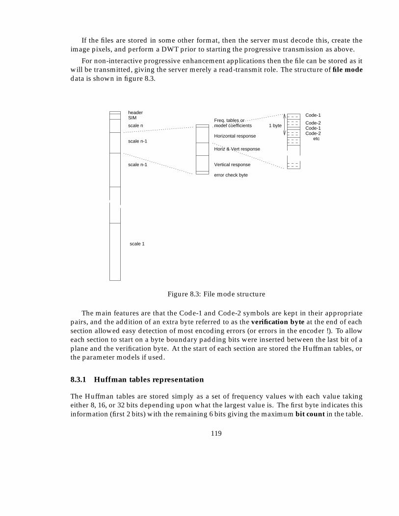
If the files are stored in some other format, then the server must decode this, create theimage pixels, and perform a DWT prior to starting the progressive transmission as above.

For non-interactive progressive enhancement applications then the file can be stored as itwill be transmitted, giving the server merely a read-transmit role. The structure of file modedata is shown in figure 8.3.

error check byte

Vertical response

Horiz & Vert response

Horizontal response

model coefficientsFreq. tables or

header

scale n

SIM

scale n-1

scale n-1

scale 1

Code-2Code-1

Code-1

1 byte

Code-2etc

Figure 8.3: File mode structure

The main features are that the Code-1 and Code-2 symbols are kept in their appropriatepairs, and the addition of an extra byte referred to as the verification byte at the end of eachsection allowed easy detection of most encoding errors (or errors in the encoder !). To alloweach section to start on a byte boundary padding bits were inserted between the last bit of aplane and the verification byte. At the start of each section are stored the Huffman tables, orthe parameter models if used.

8.3.1 Huffman tables representation

The Huffman tables are stored simply as a set of frequency values with each value takingeither 8, 16, or 32 bits depending upon what the largest value is. The first byte indicates thisinformation (first 2 bits) with the remaining 6 bits giving the maximum bit count in the table.

119

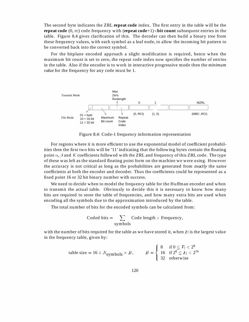
The second byte indicates the ZRL repeat code index. The first entry in the table will be therepeat code (0, rc) code frequency with (repeat code+1)�bit count subsequent entries in thetable. Figure 8.4 gives clarification of this. The decoder can then build a binary tree fromthese frequency values, with each symbol as a leaf node, to allow the incoming bit pattern tobe converted back into the correct symbol.

For the bitplane encoded approach a slight modification is required, hence when themaximum bit count is set to zero, the repeat code index now specifies the number of entriesin the table. Also if the encoder is to work in interactive progressive mode then the minimumvalue for the frequency for any code must be 1.

01 = byte10 = 16 bit11 = 32 bit

MaximumBit count

RepeatCodeIndex

File Mode

RunlengthZero Max

0 1

(1, 0)(0, RCI) (MBC ,RCI)

Transmit Mode

MZRL

Figure 8.4: Code-1 frequency information representation

For regions where it is more efficient to use the exponential model of coefficient probabil-ities then the first two bits will be ’11’ indicating that the following bytes contain the floatingpoint �, � andK coefficients followed with the ZRL and frequency of this ZRL code. The typeof these was left as the standard floating point form on the machine we were using. Howeverthe accuracy is not critical as long as the probabilities are generated from exactly the samecoefficients at both the encoder and decoder. Thus the coefficients could be represented as afixed point 16 or 32 bit binary number with success.

We need to decide when to model the frequency table for the Huffman encoder and whento transmit the actual table. Obviously to decide this it is necessary to know how manybits are required to store the table of frequencies, and how many extra bits are used whenencoding all the symbols due to the approximation introduced by the table.

The total number of bits for the encoded symbols can be calculated from:

Coded bits =X

symbolsCode length� Frequency;

with the number of bits required for the table as we have stored it, whenFl is the largest valuein the frequency table, given by:

table size = 16 +Nsymbols �B; B =

8><>:

8 if 0 � Fl < 28

16 if 28 � Fl < 216

32 otherwise

120

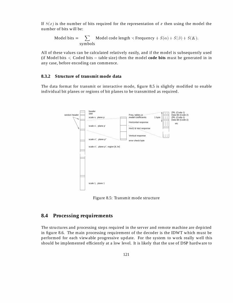
If S(x) is the number of bits required for the representation of x then using the model thenumber of bits will be:

Model bits =X

symbolsModel code length� Frequency + S(�) + S(�) + S(K):

All of these values can be calculated relatively easily, and if the model is subsequently used(if Model bits < Coded bits + table size) then the model code bits must be generated in inany case, before encoding can commence.

8.3.2 Structure of transmit mode data

The data format for transmit or interactive mode, figure 8.5 is slightly modified to enableindividual bit planes or regions of bit planes to be transmitted as required.

error check byte

Vertical response

Horiz & Vert response

Horizontal response

model coefficientsFreq. tables or

headerSIM

1 byte

etc

scale s, plane p

scale s’, plane p’

scale s’’, plane p’’

scale 1, plane 1

Data Bit (Code-2)ZRL (Code-1)

ZRL (Code-1)Data Bit (Code-2)

scale s’’, plane p’’, region [tl, br]

section header

Figure 8.5: Transmit mode structure

8.4 Processing requirements

The structures and processing steps required in the server and remote machine are depictedin figure 8.6. The main processing requirement of the decoder is the IDWT which must beperformed for each viewable progressive update. For the system to work really well thisshould be implemented efficiently at a low level. It is likely that the use of DSP hardware to

121

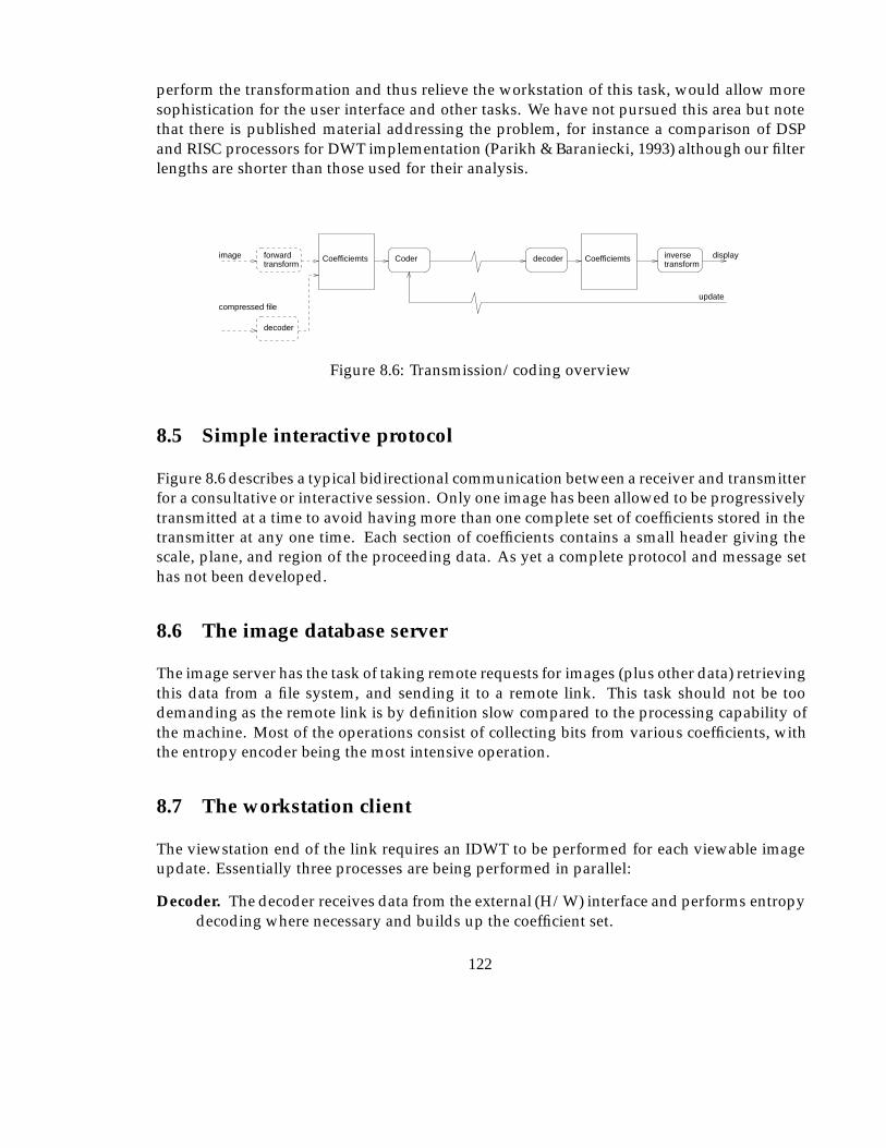
perform the transformation and thus relieve the workstation of this task, would allow moresophistication for the user interface and other tasks. We have not pursued this area but notethat there is published material addressing the problem, for instance a comparison of DSPand RISC processors for DWT implementation (Parikh & Baraniecki, 1993) although our filterlengths are shorter than those used for their analysis.

inversetransform

Coder decoder

decoder

transformforward Coefficiemts displayimage

update

Coefficiemts

compressed file

Figure 8.6: Transmission/coding overview

8.5 Simple interactive protocol

Figure 8.6 describes a typical bidirectional communication between a receiver and transmitterfor a consultative or interactive session. Only one image has been allowed to be progressivelytransmitted at a time to avoid having more than one complete set of coefficients stored in thetransmitter at any one time. Each section of coefficients contains a small header giving thescale, plane, and region of the proceeding data. As yet a complete protocol and message sethas not been developed.

8.6 The image database server

The image server has the task of taking remote requests for images (plus other data) retrievingthis data from a file system, and sending it to a remote link. This task should not be toodemanding as the remote link is by definition slow compared to the processing capability ofthe machine. Most of the operations consist of collecting bits from various coefficients, withthe entropy encoder being the most intensive operation.

8.7 The workstation client

The viewstation end of the link requires an IDWT to be performed for each viewable imageupdate. Essentially three processes are being performed in parallel:

Decoder. The decoder receives data from the external (H/W) interface and performs entropydecoding where necessary and builds up the coefficient set.

122

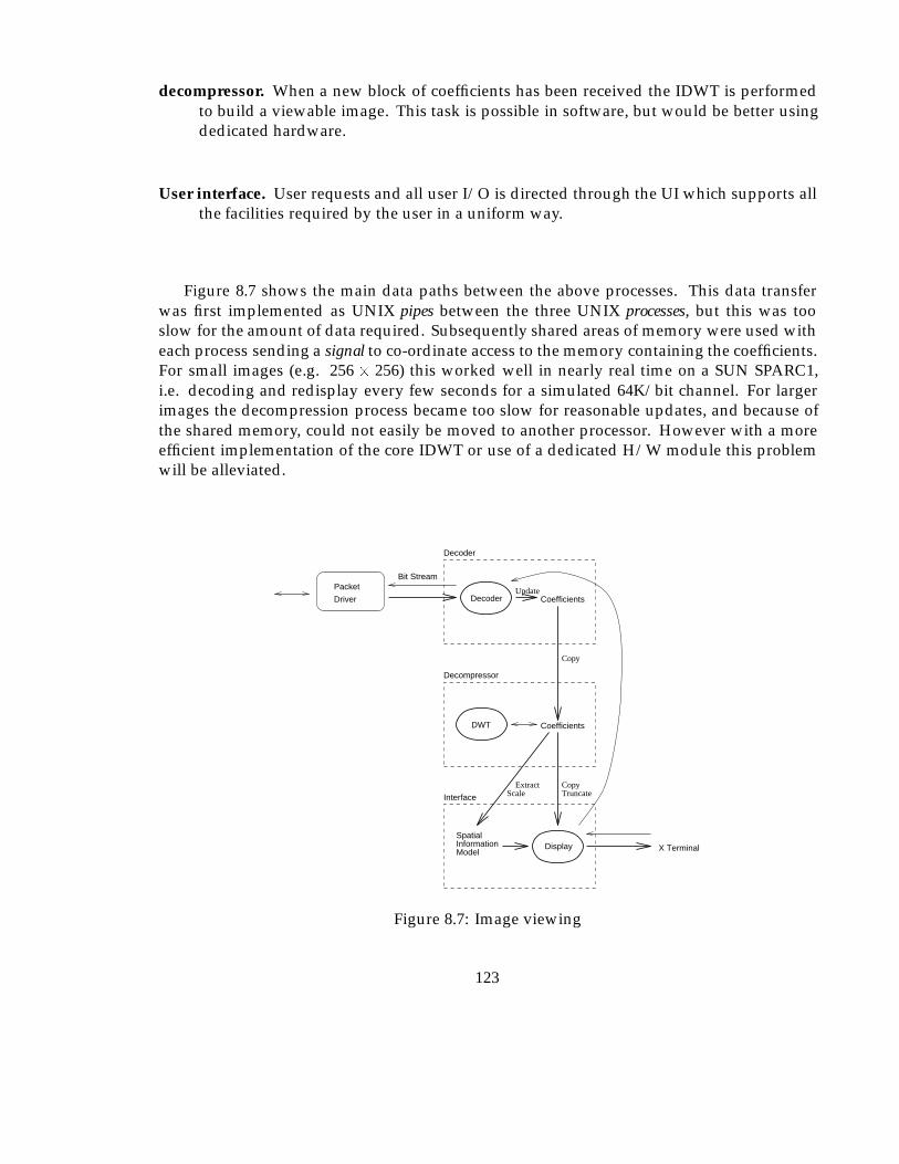
decompressor. When a new block of coefficients has been received the IDWT is performedto build a viewable image. This task is possible in software, but would be better usingdedicated hardware.

User interface. User requests and all user I/O is directed through the UI which supports allthe facilities required by the user in a uniform way.

Figure 8.7 shows the main data paths between the above processes. This data transferwas first implemented as UNIX pipes between the three UNIX processes, but this was tooslow for the amount of data required. Subsequently shared areas of memory were used witheach process sending a signal to co-ordinate access to the memory containing the coefficients.For small images (e.g. 256 � 256) this worked well in nearly real time on a SUN SPARC1,i.e. decoding and redisplay every few seconds for a simulated 64K/bit channel. For largerimages the decompression process became too slow for reasonable updates, and because ofthe shared memory, could not easily be moved to another processor. However with a moreefficient implementation of the core IDWT or use of a dedicated H/W module this problemwill be alleviated.

SpatialInformationModel

CoefficientsUpdate

Copy

Coefficients

CopyExtractScale TruncateInterface

Decompressor

X TerminalDisplay

DWT

Decoder

Bit StreamPacket

Driver

Decoder

Figure 8.7: Image viewing

123

8.8 Comment

The key parts of the image transmission system were implemented, with a simple mock upuser interface, supporting only those functions relevant to the operation of the transmissionand compression algorithms.

124

Chapter 9

Conclusions and Future Work

9.1 Introduction

This final chapter presents a discussion of some of the aspects of what has been done. Wherefurther work is still to be done to complete the objectives, this is noted, along with possibledirections for future work and in some instances our expectations of results. Obviously anyitems for which results have not previously been given are tentative, though the reasoningwhich has lead to these expectations is given where possible.

9.2 Discussion

9.2.1 Wavelet encoding of imagery

In the process of designing a quantization strategy the goal is to minimise distortion within thereconstructed image. The most commonly adopted approach is to attempt to minimise someempirical measure, typically MSE or SNR. Although generally an image with a high SNR,for instance, will be of subjectively good quality, when we start placing stringent conditionsupon the visual integrity of the image these simple measures do not necessarily reflect thedetail which can be extracted from the image by the human visual system. The problemhas been approached from the opposite direction and the image is encoded according towhat is known about the way the visual system acts. The resultant empirical measures showthe system to be competitive with current state of the art methods, and the appearance anddetailed examination of the resultant images appears to be superior (although we have notverified this statistically with an ROC study yet).

It is quite obvious that the blocking artefacts which become obvious in some blockedtransforms at high compression do not appear in the same regular form, though of coursedistortion is produced by the narrow filter DWT at high ratios, however it can be argued thatit is of a less distracting form to the visual system. The other main identifiable distortion

125

artefact, known as ‘ringing’ or false edges around sharp contrast changes (HF components)is also reduced in the DWT due to the localisation of the domain of each coefficient.

We believe that the application of the contrast masking curve improved the visibility of finedetail for a given compression ratio to a greater extent than suggested by the SNR measure.This is particularly true for medium ratios where the SNR and APE measures becomerelatively poor, though the visual quality is good, and appears to contain greater detail.It was gratifying to note that similar conclusion and quantization strategy between scales hassince been reached by another researcher through a rigorous mathematical derivation of asimilar problem (DeVore et al., 1992).

Considering the low quality part of figure 7.8 reproduced as figure 9.1 the bitplaneapproach and CM give the same SNR, though the CM has superior visibility for fine detail.These two curves diverge at about 0.6bpp due to the NLQ producing errors for large valuescoefficients, though these are not visible. The NLQ reaches a maximum quality because ofthis and should have the linearity of the quantizer increased for lower ratios, it would thenfollow the SNR for the bitplane approach, which ultimately becomes integer rounding atabout 4 bpp.

9.2.2 Progressive enhancement

Progressive enhancement has been presented as an important feature of our solution thoughit is true that progressive enhancement will always be an imperfect but important enablingtechnology. In any situation where the user is involved directly in the enhancement process itis a work around solution, as ideally instant full quality display is preferable. There are a fewsituations where enhancement can be utilised unknown to the user as noted in section 3.10.1.However if this technology can be used to widen availability of images and thus providebenefit in, for instance, rural areas, then it has been worth the effort.

It was not a surprise to have read very little in the literature concerning the progressiveenhancement of medical images, mainly because the scenarios where we expect it to beuseful simply do not currently consider the possibility of having images available. It istherefore impossible to judge the effect of this strategy on the user. We believe it is very mucha technology to enable experiments concerning the wider availability of medical images,especially in rural areas and where smaller more localised hospitals can provide better careby allowing aspects of diagnosis which do not require direct patient interaction performedremotely.

9.2.3 Frequency table models

Using the exponential model to create the Huffman decoding tables was found to give a closerresults to the actual frequency tables for the interactive progressive enhancement situation.The reason for this is due to the requirement for a symbol to be available for every possibleCode-1, as the actual codes are not known when the tables are generated.

126

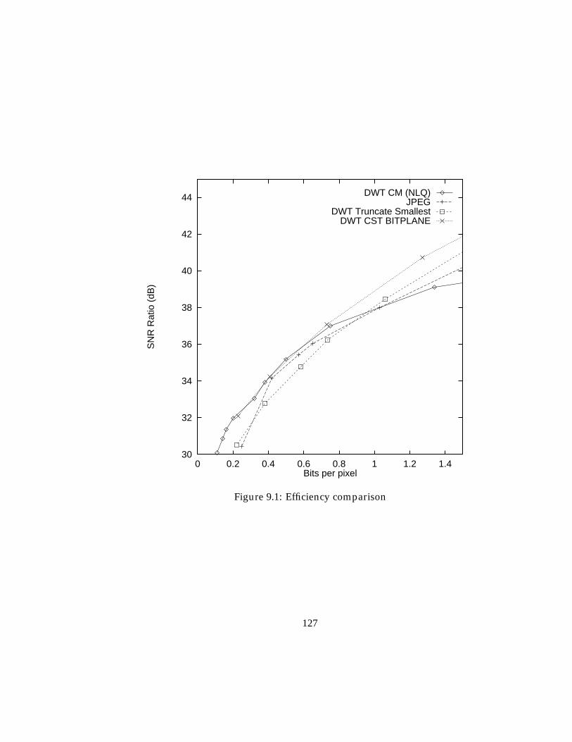
30

32

34

36

38

40

42

44

0 0.2 0.4 0.6 0.8 1 1.2 1.4

SN

R R

atio

(dB

)

Bits per pixel

DWT CM (NLQ)JPEG

DWT Truncate SmallestDWT CST BITPLANE

Figure 9.1: Efficiency comparison

127

The actual frequency tables are not critical to the efficiency of the Huffman algorithm, inthe sense that an approximation will often produce identical length codes for each symbol.Clearly, though it is important that a receiver can construct exactly the same bits for eachsymbol. Therefore, if a model is to be used and particularly if it is specified by real coefficients,the encoder/decoder must be able to calculate the same approximate frequency tables. Toensure this, the encoder having found a suitable model, limits the accuracy of the coefficientsto a specified level, and calculates the frequencies which are then used to encode the symbols.Providing that the calculation of the frequency tables from the model produce the same resultswhen rounded to integer values the decoder will function correctly.

As yet it is not clear how it is possible to determine when the model should be usedwithout first generating the Huffman tables (or at least the number of bits in each) for themodel. The processing to generate the table is not too great,and so this possibility has notbeen investigated further, as a ‘trial and error’ approach is satisfactory..

9.2.4 Visual models

CST and CM have been utilised to improve the quantization strategy for the encodingalgorithm. There is another visual characteristic concerned with the visual detection thresholdat differing intensity values. The effects reproduced in the context of digital radiology (Sezanet al., 1987) show that the eye is more sensitive at low to mid intensity ranges. Sezan utilisednon uniform quantization based on this to allow 8 bit quantization of 12 bit images, with agood deal of success.

To apply this to the DWT would require modification of the quantizer based upon theaverage intensity of the region within which each coefficient is represented. It is likelythat the smoothed S2j coefficients could be utilised for this, however this has not beeninvestigated yet because of the complication of integrating this together with the CM nonuniform characteristic. A second reason for avoiding this possibility is that according to arecent report (Cox et al., 1992) such an approach can give radiologists the impression of a ‘flat’and ‘unfamiliar’ image.

9.2.5 Anatomic models

In the future higher level processing of the images based upon knowledge about the acqui-sition, structure, anatomy and variability of the various images will allow better and fastersegmentation of the images. Other systems currently within the scope of AI research willallow the optimum compression to be created for each image dependent on a multitude offactors.

9.2.6 Application to other fields

Medical images have been the only concern of this work. There are many other specialistimage related applications which might benefit from reduced bandwidth requirements. The

128

basic strategy of the approach, and indeed the DWT should be applicable to most ‘natural’image types, with the higher level information including object models and heuristics typicallybeing generated specifically for the application.

If only the DWT quantization and progressive enhancement, details are consideredapplications such as remote picture database browsers are possible. Some features suchas the fast viewing of SIMS to allow the user to make more informed decisions about imagecontent before downloading large images, are easily supported.

9.2.7 Runlength encoding

To avoid producing many infrequently used runlength codes we have used a repeat code forproducing longer runlength sequences. This length has been somewhat arbitrarily chosen as15 for the implementation. By making the RC larger then less RC symbols will be generated, atthe expense of having more infrequently used run length codes. Investigation of the optimalrun length repeat code has not been performed yet.

9.3 Important future additions

The following sections describe some aspects which we have not addressed, but which areimportant to the area. Possible directions for study of these are noted where appropriate.

9.3.1 Multi frame images

The primary consideration in this work has been computed radiography applications, manyof the concepts however will apply to most other modalities. When there is an obvious extradimension to the data set, usually either a time sequence of images, or a number of spatialslices of an object it is necessary to utilise the potentially very large correlation between theseimages. A recent paper (Lee et al., 1993), which has investigated compression of CT imagesbased on the blocked DCT showed significant improvements in quality from the inter slicecompared with standard intra slice methods. The paper had two intriguing results, firstlythe SNR of the new method was no better than the inter slice version, and secondly readersreported better quality perceived for 5:1 compressed images than the originals though nodifference in ROC was found. For this latter phenomena, a similar result appeared in ourwork for single images and was attributed to the removal of some HF noise by the compressionalgorithm.

The extension to multi slice data using the DWT has not been pursued although there isan exciting possibility for a large improvement in compression ratios for such data using a 3dimensional version of the DWT algorithm. The possibility of extending the transform itselfto three dimensions (i.e. filtering on X, then Y, then Z and thus creating a ‘cube’ of coefficientspace with 8 regions for each transform level), should be possible given the orthogonality of the

129

transform. This would allow quantization between frames, so we could consider for instance,HF vertical components which have changed a large amount since the last frame, and thosewhich have remained static. Therefore, the changes between frames at each resolution wouldbecome apparent from the coefficients and we could quantize accordingly. For applicationslike time sequences of images when a contrast dye is used this detail is particularly relevant.

9.3.2 Colour images

Colour images have not been considered as the majority of medical images are monochrome,though some have artificial colour added at a later date. It will be possible to include a colourcomponent by encoding each colour channel (RGB or YUV) with a separate DWT. Otherwell known features such as limiting colour resolution more than intensity resolution can beutilised.

9.4 Conclusions

It is clear that the only acceptable method of evaluating the subject matter of this work,prior to use in real medical situations is through ROC studies. This in turn would require afull implementation of the system or functionally equivalent prototype. The work involvedwould be substantial, specifically there are a few areas which still have to be fully addressedto obtain the performance that we would like to achieve from the system.

To perform such a study would require the involvement of a substantial number of medicalstaff, the use of expensive, already over utilised (where it exists) medical equipment.

This level of implementation has not been possible, but it was never the intention. Theoriginal aim was to determine if it might be feasible to use the ISDN for diagnostic imagingtasks. From the beginning it was apparent that compression of the data as well as howit is accessed were expected to be key issues, and given that most general methods wereunsuitable, we were interested to try and find modifications, or other techniques which mightprovide better results.

It is evident that the laws of information theory predict that the only way to improvecompression ratios without losing quality, is to restrict the possible images the system couldcompress thereby placing more of the image information within the encoder/ decoder. It wasclear that medical images are definitely a small class of all possible images, but exactly howto identify these characteristics and use them to our advantage is a difficult problem indeed.The basic strategy would seem to be to characterise or model each image type to enable adecoder to effectively make ‘assumptions’ due to information it can be equipped with. Inaddition, if we are to compress beyond the redundancy (entropy), and as our models will bynecessity only be crude due to the range of variability within images which it is required torepresent, something will inevitably be lost. We consider that there are another two levels ofredundancy (redundant in the sense of not required for the purposes of the application).

130

Firstly, when carefully applied, the limitations of the human visual system can be utilisedto remove information which cannot be seen (processed) by the observer. It is importantto realise that with modern image processing these details can sometimes be made visible,indeed many processing techniques work, by moving details into the sensitive region of theHVS. Obviously care must be taken to cater for this situation.

Secondly, it is sometimes possible to identify ‘macro redundancy’ in terms of the actualcomposition or structures within the image and their contribution to the subsequent diagnostictask. We have only considered the crudest, being the noisy background found on manyimages, and for most applications considered to be of zero value, and thus redundant. Becauseof the number of varying results in the literature considering quality requirements for variousimage types, structures within images and observer expectations, we feel sure that additionalmore subtle macro redundancies can be found for some types of image. To utilise such ideasmodel based segmentation and labelling utilising domain knowledge to constrain locationof the structure of the image would be required. Following this AI techniques such as casereasoning, and expert systems, could be used on these higher level abstractions of the imagestructure to determine optimum compression efficiency for each region.

To utilise techniques such as these we have chosen to use the DWT to redistribute theenergy into a space where the HVS model can be utilised, and potentially some simple macroredundancy in terms of regions as well. The Huffman encoder, though not a state of the artlossless encoder provides good results at low cost, to remove residual correlation.

Looking well into the future it becomes reasonable that compression systems, and ‘auto-mated image readers1’ would converge in the sense that abnormalities would be the part ofan image which the compression routine could not (or would not) compress well (it wouldeither have a good model, or spot as detail not required, for everything else). Of coursethe compression itself would then become redundant as only the textual ‘radiologists report’would need to be stored !

At the conclusion of the experiments performed in this work it has become clear thatthere are benefits to be obtained in terms of economy and quality when transmitting andarchiving such data. Although there are many parts of this work which could be developedfurther before an operational system is built, the effect of using general lossy image encodingalgorithms might well be considered a false economy.

1some experiments are being carried out in spotting specific abnormalities (cancer growths), and in (Dallas &Roehrig, 1987) to locate vessels in soft tissue

131

Appendix A

Appendix A: Algorithms

A.1 � estimation

To find the value of � (Section 6.7.4.3) a simple iterative algorithm was used which repeatedlyadds or subtracts an error factor, which itself is halved whenever the sign of the error betweenthe real and modelled distributions changes.

An estimated value of � is produced by considering the gradient of the line joining thetwo samples either side of the value closest to the 1=e point on the curve. The estimate isusually within �1 so 0.5 is used as the initial increment.

� estimationset adjustment to 0.5while � not accurate enough

calculate error between real distribution and model using current � and �.if the error has a different sign then

reduce the adjustment by 50% and change its signotherwise

if the error is greater magnitude than last time thenchange the sign of the adjustment amount

add adjustment to �

The actual implementation has a few additional checks which allow a maximum numberof iterations (20) to be set. The error is the total difference between the real and modelleddistributions for non zero values of the real distribution. i.e.

P(P (i)�Ke�(juj=�)

�

) forP (i) 6= 0.

A.2 Forward transform code

The following constants are defined globally:

132

C0 = (1+sqrt(3.0))/8.0*sqrt(2.0);C1 = (3+sqrt(3.0))/8.0*sqrt(2.0);C2 = (3-sqrt(3.0))/8.0*sqrt(2.0);C3 = (1-sqrt(3.0))/8.0*sqrt(2.0);

Code to perform one layer of the two dimensional DWT transform./*--------------------------------------------------------------------------*/

void wavelet_transform(size)/*--------------------------------------------------------------------------*/

int size;{p_type *column_ptr, *row_ptr;int i,j;

column_ptr = parameters_out;row_ptr = parameters_in;for (i=0; i<size; i++){daub4(row_ptr, column_ptr, column_ptr+(NUMBER_COEFFICIENTS*size/2), size);row_ptr += NUMBER_COEFFICIENTS;column_ptr++;

}column_ptr = parameters_in;row_ptr = parameters_out;for (i=0; i<size; i++){daub4(row_ptr, column_ptr, column_ptr+(NUMBER_COEFFICIENTS*size/2), size);row_ptr += NUMBER_COEFFICIENTS;column_ptr++;

}}

Calculate one column of the output (input from one row of the input). The input ptrpoints to a row of data to be transformed, the output ptr points to the top of the output row(smooth part) the row size is the offset to add to get an element 1 row below the current./*--------------------------------------------------------------------------*/

void daub4(input_ptr, smooth_ptr, detail_ptr, size)/*--------------------------------------------------------------------------*/

p_type *input_ptr, *smooth_ptr, *detail_ptr;int size;{p_type *sav_ptr;int i;sav_ptr = input_ptr;

for (i=0; i<(size-2); i+=2){

*smooth_ptr = (p_type)(*input_ptr*C0 + *(input_ptr+1)*C1 +*(input_ptr+2)*C2 + *(input_ptr+3)*C3);

*detail_ptr = (p_type)(*input_ptr*C3 + *(input_ptr+1)*-C2 +

133

*(input_ptr+2)*C1 + *(input_ptr+3)*-C0);

detail_ptr += NUMBER_COEFFICIENTS;smooth_ptr += NUMBER_COEFFICIENTS;input_ptr += 2;

}

*smooth_ptr = (p_type)(*sav_ptr*C2 + *(sav_ptr+1)*C3 +*(input_ptr)*C0 + *(input_ptr+1)*C1);

*detail_ptr =(p_type)(*sav_ptr*C1 + *(sav_ptr+1)*-C0 +*(input_ptr)*C3 + *(input_ptr+1)*-C2);

}

To perform a complete decomposition leaving smooth coefficients determined by the valueof THE END.

/*--------------------------------------------------------------------------*/void wavelet_coder()

/*--------------------------------------------------------------------------*/{static int size;

size = image_size;while (size > THE_END ) {wavelet_transform(size);size = size/2;

}}

A.3 IDWT Code

Perform one layer of the inverse DWT transform./*--------------------------------------------------------------------------*/

void inverse_wt(size, param_source)/*--------------------------------------------------------------------------*/

int size; p_type *param_source;{p_type *column_ptr, *row_ptr;int i,j;

column_ptr = param_source;row_ptr = parameters_store;for (i=0; i<size; i++){inverse_daub4(row_ptr, column_ptr, column_ptr+(size/2), size);row_ptr++;column_ptr += NUMBER_COEFFICIENTS;

}

134

column_ptr = parameters_store;row_ptr = parameters_out;for (i=0; i<size; i++){inverse_daub4(row_ptr, column_ptr, column_ptr+(size/2), size);row_ptr++;column_ptr += NUMBER_COEFFICIENTS;

}}

The following routine is the inverse of daub4./*--------------------------------------------------------------------------*/

void inverse_daub4(output_ptr, smooth_ptr, detail_ptr, size)/*--------------------------------------------------------------------------*/

p_type *output_ptr, *smooth_ptr, *detail_ptr;int size;{p_type *sav_smooth_ptr, *sav_detail_ptr, *sav_output_ptr;int i;

sav_smooth_ptr = smooth_ptr;sav_detail_ptr = detail_ptr;sav_output_ptr = output_ptr;

output_ptr += 2*NUMBER_COEFFICIENTS;

for (i=2; i<size; i+=2){*output_ptr = (p_type)(*smooth_ptr*C2 + *detail_ptr*C1 +

*(smooth_ptr+1)*C0 + *(detail_ptr+1)*C3);output_ptr += NUMBER_COEFFICIENTS;

*output_ptr = (p_type)(*smooth_ptr*C3 + *detail_ptr*-C0 +*(smooth_ptr+1)*C1 + *(detail_ptr+1)*-C2);

output_ptr += NUMBER_COEFFICIENTS;detail_ptr++;smooth_ptr++;

}*sav_output_ptr = (p_type)(*sav_smooth_ptr*C0 + *sav_detail_ptr*C3 +

*smooth_ptr*C2 + *detail_ptr*C1);sav_output_ptr += NUMBER_COEFFICIENTS;

*sav_output_ptr = (p_type)(*sav_smooth_ptr*C1 + *sav_detail_ptr*-C2 +*smooth_ptr*C3 + *detail_ptr*-C0);

}

The routine to generate an image from a complete set of coefficients. A duplicate set ofcoefficients is used to avoid corrupting the coefficient set in case of progressive enhancement./*--------------------------------------------------------------------------*/

void wavelet_decoder(parameters_in)

135

p_type *parameters_in;/*--------------------------------------------------------------------------*/

{

int size;

size = image_size;while (size > THE_END && (size % 2) == 0) {size = size/2;

}memcpy(parameters_out, parameters_in, NUMBER_COEFFICIENTS*NUMBER_COEFFICIENTS*sizeof(p_type));

size = size*2;inverse_wt(size, parameters_in); /* result in parameters_out */

while (size < image_size) {size = size*2;inverse_wt(size, parameters_out); /* result in parameters_out */

}}

A.4 Encoder

The basic encoder used the send symbols routine to transmit the Code 1 data. This in turnutilises the storecode routine to accumulate the various bits into bytes. The codebits and lenarrays provide the coded form of each symbol and the number of bits required respectively.

/*--------------------------------------------------------------------------*/void send_symbols(location, outputfile)struct area *location;FILE *outputfile;

/*--------------------------------------------------------------------------*/{int j, k, h, h1, zero_run;int s1;

zero_run = 0;storecode(0, 0, ’s’, outputfile); /* reset bitstream */for (j=location->upper_left.y; j<location->lower_right.y; j++)for (k=location->upper_left.x; k<location->lower_right.x; k++) {

h = (int)*(parameters_in+((k)*NUMBER_COEFFICIENTS)+j);if ((h == 0) && (zero_run<(run_bits-1)))

zero_run++;else {

136

storecode(bits_in(h), zero_run, ’n’, outputfile);zero_run = 0; }

*(size+((k)*NUMBER_COEFFICIENTS)+j) = (int)(1<<bits_in(h))>>1;if (h<0)*(parameters_in+((k)*NUMBER_COEFFICIENTS)+j) = (p_type)(h-1);

}storecode(0, run_bits-1, ’n’, outputfile); /*over run with repeat code*/storecode(0, 0, ’c’, outputfile); /* finish current byte */}

/*--------------------------------------------------------------------------*/void storecode(nbits, zero_run, mode, outputfile)

/*--------------------------------------------------------------------------*/int nbits, zero_run;char mode;FILE *outputfile;{static int bits_fill, outbyte;unsigned int code_bits, code_symbol, bitsctr, mask;int code_index, num_bits;

switch (mode) {case ’c’ : if (bits_fill != 0){

if (bits_fill <8)outbyte = outbyte << (8-bits_fill);

fputc(outbyte, outputfile);}fputc(sync_byte, outputfile); /* write a check

byte */break;

case ’s’ : outbyte = bits_fill = 0;break;

case ’n’ : code_index = nbits*run_bits+zero_run;

code_bits = len[code_index];mask = 1 << (code_bits-1);code_symbol = codebits[code_index];

for (bitsctr=0; bitsctr<code_bits; bitsctr++){if ((code_symbol & mask )==0)

outbyte = outbyte << 1;elseoutbyte = (outbyte << 1)+1;

mask = mask >>1;bits_fill += 1;

if (bits_fill == 8) {fputc(outbyte, outputfile);

137

outbyte = bits_fill = 0;}

}}

}

The following two procedures collect and send the actual coefficient data (Code 2) for aspecific region.

/*--------------------------------------------------------------------------*/void send_coefficients(location, outputfile)

/*--------------------------------------------------------------------------*/struct area *location;FILE* outputfile;{int j, k, h;

store_coefficient(0, 0, ’s’, outputfile); /* reset bitstream */

for (j=location->upper_left.y; j<location->lower_right.y; j++)for (k=location->upper_left.x; k<location->lower_right.x; k++) {

h = (int)*(parameters_in+((k)*NUMBER_COEFFICIENTS)+j);

if (*(size+((k)*NUMBER_COEFFICIENTS)+j) > 0){store_coefficient(h, size+((k)*NUMBER_COEFFICIENTS)+j,’n’, outputfile);

}}

store_coefficient(0, 0, ’c’, outputfile); /* finish current byte */}

/*--------------------------------------------------------------------------*/void store_coefficient(h, bits_left, mode, outputfile)

/*--------------------------------------------------------------------------*/int *bits_left, h;char mode;FILE *outputfile;{static int bits_fill, outbyte;unsigned int code_bits, code_symbol, bitsctr, mask;int code_index, num_bits;

switch (mode) {case ’c’ : if (bits_fill != 0){

if (bits_fill <8)outbyte = outbyte << (8-bits_fill);

fputc(outbyte, outputfile);}

138

fputc(sync_byte,outputfile); /* write a check for debug*/break; /* wavelet_module.c */

case ’s’ : outbyte = bits_fill = 0;break;

case ’n’ :mask = *bits_left;for (bitsctr=0; (mask!=0); bitsctr++){if ((h & mask)==0)outbyte = outbyte << 1;

elseoutbyte = (outbyte << 1)+1;

mask = mask >>1;bits_fill += 1;if (bits_fill == 8) {fputc(outbyte, outputfile);outbyte = bits_fill = 0;

}

*bits_left = mask;}

}}

A.5 Decoder

The following is the receiver version of send symbols. Tree is the Huffman decoder tree rootnode from which the symbols are recovered as each bit is received.

/*--------------------------------------------------------------------------*/void get_symbols(tree, location, inputfile)

/*--------------------------------------------------------------------------*/struct hnode *tree;struct area *location;FILE *inputfile;{int j, k, h1, length, zero_run;unsigned int symbol, mask;

mask = 128;zero_run = 0;getcode(tree, ’s’, inputfile); /* reset input */symbol = getcode(tree, ’n’, inputfile);length = symbol >> run_no_bits;zero_run = symbol % run_bits;

for (j=location->upper_left.y; j<location->lower_right.y; j++)

139

for (k=location->upper_left.x; k<location->lower_right.x; k++) {

if (zero_run==0){*(size+((k)*NUMBER_COEFFICIENTS)+j) = (1<<length)>>1;symbol = getcode(tree, ’n’, inputfile);length = symbol >> run_no_bits;zero_run = symbol % run_bits;}

else {*(size+((k)*NUMBER_COEFFICIENTS)+j) = 0;zero_run--; }

}getcode(tree, ’s’, inputfile); /* reset input */getcode(tree, ’y’, inputfile); /* check sync byte */}

/*--------------------------------------------------------------------------*/unsigned int getcode( tree, mode, inputfile)

/*--------------------------------------------------------------------------*/struct hnode *tree;char mode;FILE *inputfile;{struct hnode *tree_climber;static int inbyte, length, bitsctr;static unsigned int symbol, mask;

tree_climber = tree;switch (mode) {case ’s’ : inbyte = mask = symbol = 0;

break;case ’y’ : inbyte = fgetc(inputfile);

if (inbyte != sync_byte)printf("found incorrect symbol-1 sync byte %c=%d\n",inbyte, inbyte);symbol = 0;break;

case ’n’ :symbol = -2;do{if (mask == 0) {inbyte = fgetc(inputfile);mask = 128; }

if ((inbyte & mask) == 0){if (tree_climber->zero == NULL)symbol = tree_climber->data_zero;

elsetree_climber = tree_climber->zero; }

else {

140

if (tree_climber->one == NULL)symbol = tree_climber->data_one;

elsetree_climber = tree_climber->one; }

mask = mask >> 1;}while (symbol == -2);

}if (symbol == -1) halt("error reading input");return symbol;

}

The get coefficients routine is the receive version of send coefficients and builds up eachcoefficient as the data is received.

/*--------------------------------------------------------------------------*/void get_coefficients(location, inputfile)

/*--------------------------------------------------------------------------*/struct area *location;FILE *inputfile;{int j, k;

load_coefficient(NULL, 0, ’s’, inputfile); /* reset input */

for (j=location->upper_left.y; j<location->lower_right.y; j++)for (k=location->upper_left.x; k<location->lower_right.x; k++) {if (*(size+((k)*NUMBER_COEFFICIENTS)+j)>0)load_coefficient((size+((k)*NUMBER_COEFFICIENTS)+j),(parameters_in+((k)*NUMBER_COEFFICIENTS)+j), ’n’, inputfile);

}

load_coefficient(0, 0, ’s’, inputfile); /* reset input */load_coefficient(0, 0, ’y’, inputfile); /* check sync byte */}

There is obviously a large amount of additional code required to produce a workablesystem, the above gives an outline of the key low procedures in the basic DWT and en-coder/decoder.

141

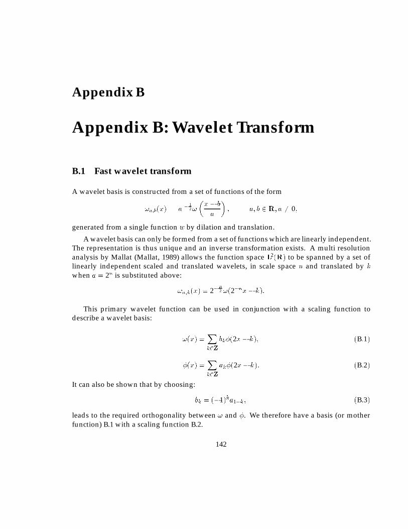
Appendix B

Appendix B: Wavelet Transform

B.1 Fast wavelet transform

A wavelet basis is constructed from a set of functions of the form

!a;b(x) = jaj� 12!

�x � b

a

�; a; b 2 R; a 6= 0;

generated from a single function w by dilation and translation.

A wavelet basis can only be formed from a set of functions which are linearly independent.The representation is thus unique and an inverse transformation exists. A multi resolutionanalysis by Mallat (Mallat, 1989) allows the function space L2(R) to be spanned by a set oflinearly independent scaled and translated wavelets, in scale space n and translated by k

when a = 2n is substituted above:

!n;k(x) = 2�n2 !(2�nx� k):

This primary wavelet function can be used in conjunction with a scaling function todescribe a wavelet basis:

!(x) =Xk2Z

bk�(2x� k); (B:1)

�(x) =Xk2Z

ak�(2x� k): (B:2)

It can also be shown that by choosing:

bk = (�1)ka1�k ; (B:3)

leads to the required orthogonality between ! and �. We therefore have a basis (or motherfunction) B.1 with a scaling function B.2.

142

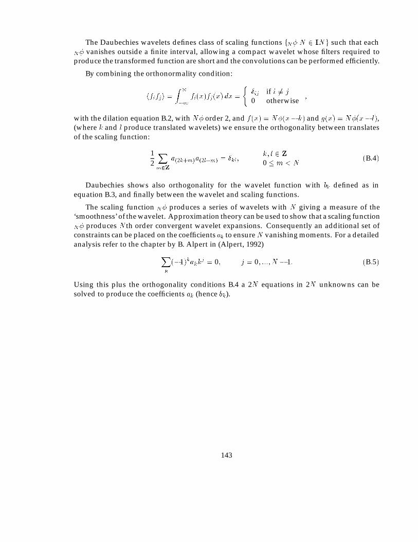
The Daubechies wavelets defines class of scaling functions fN�jN 2 INg such that eachN� vanishes outside a finite interval, allowing a compact wavelet whose filters required toproduce the transformed function are short and the convolutions can be performed efficiently.

By combining the orthonormality condition:

hfifji =Z 1

�1fi(x)fj(x) dx =

(�ij if i 6= j

0 otherwise;

with the dilation equation B.2, with N� order 2, and f(x) = N�(x� k) and g(x) = N�(x� l),(where k and l produce translated wavelets) we ensure the orthogonality between translatesof the scaling function:

12

Xm2Z

a(2k+m)a(2l+m) = �kl;k; l 2 Z0 � m < N

(B:4)

Daubechies shows also orthogonality for the wavelet function with bk defined as inequation B.3, and finally between the wavelet and scaling functions.

The scaling function N� produces a series of wavelets with N giving a measure of the‘smoothness’ of the wavelet. Approximation theory can be used to show that a scaling functionN� produces N th order convergent wavelet expansions. Consequently an additional set ofconstraints can be placed on the coefficients ak to ensureN vanishing moments. For a detailedanalysis refer to the chapter by B. Alpert in (Alpert, 1992)

Xk

(�1)kakkj = 0; j = 0; :::; N � 1: (B:5)

Using this plus the orthogonality conditions B.4 a 2N equations in 2N unknowns can besolved to produce the coefficients ak (hence bk).

143

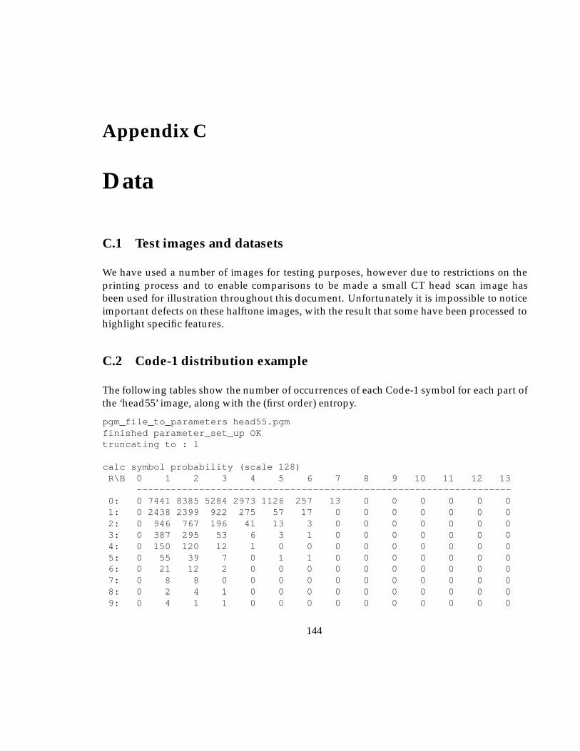
Appendix C

Data

C.1 Test images and datasets

We have used a number of images for testing purposes, however due to restrictions on theprinting process and to enable comparisons to be made a small CT head scan image hasbeen used for illustration throughout this document. Unfortunately it is impossible to noticeimportant defects on these halftone images, with the result that some have been processed tohighlight specific features.

C.2 Code-1 distribution example

The following tables show the number of occurrences of each Code-1 symbol for each part ofthe ‘head55’ image, along with the (first order) entropy.

pgm_file_to_parameters head55.pgmfinished parameter_set_up OKtruncating to : 1

calc symbol probability (scale 128)R\B 0 1 2 3 4 5 6 7 8 9 10 11 12 13

------------------------------------------------------------------0: 0 7441 8385 5284 2973 1126 257 13 0 0 0 0 0 01: 0 2438 2399 922 275 57 17 0 0 0 0 0 0 02: 0 946 767 196 41 13 3 0 0 0 0 0 0 03: 0 387 295 53 6 3 1 0 0 0 0 0 0 04: 0 150 120 12 1 0 0 0 0 0 0 0 0 05: 0 55 39 7 0 1 1 0 0 0 0 0 0 06: 0 21 12 2 0 0 0 0 0 0 0 0 0 07: 0 8 8 0 0 0 0 0 0 0 0 0 0 08: 0 2 4 1 0 0 0 0 0 0 0 0 0 09: 0 4 1 1 0 0 0 0 0 0 0 0 0 0

144

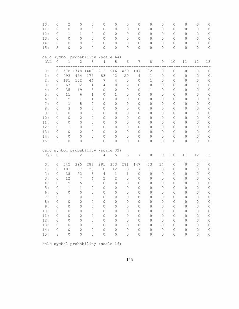
10: 0 2 0 0 0 0 0 0 0 0 0 0 0 011: 0 0 0 0 0 0 0 0 0 0 0 0 0 012: 0 1 1 0 0 0 0 0 0 0 0 0 0 013: 0 0 0 0 0 0 0 0 0 0 0 0 0 014: 0 0 0 0 0 0 0 0 0 0 0 0 0 015: 3 0 0 0 0 0 0 0 0 0 0 0 0 0

calc symbol probability (scale 64)R\B 0 1 2 3 4 5 6 7 8 9 10 11 12 13

------------------------------------------------------------------0: 0 1578 1748 1408 1213 916 439 107 32 0 0 0 0 01: 0 493 454 175 83 42 20 4 1 0 0 0 0 02: 0 181 152 44 7 4 0 0 1 0 0 0 0 03: 0 67 62 11 4 0 2 0 0 0 0 0 0 04: 0 35 19 5 0 0 0 0 1 0 0 0 0 05: 0 11 6 1 0 1 0 0 0 0 0 0 0 06: 0 5 1 1 0 0 0 0 0 0 0 0 0 07: 0 1 5 0 0 0 0 0 0 0 0 0 0 08: 0 3 0 0 0 0 0 0 0 0 0 0 0 09: 0 0 0 0 0 0 0 0 0 0 0 0 0 010: 0 0 0 0 0 0 0 0 0 0 0 0 0 011: 0 0 0 0 0 0 0 0 0 0 0 0 0 012: 0 1 0 0 0 0 0 0 0 0 0 0 0 013: 0 0 0 0 0 0 0 0 0 0 0 0 0 014: 0 0 0 0 0 0 0 0 0 0 0 0 0 015: 3 0 0 0 0 0 0 0 0 0 0 0 0 0

calc symbol probability (scale 32)R\B 0 1 2 3 4 5 6 7 8 9 10 11 12 13

------------------------------------------------------------------0: 0 345 395 288 291 333 281 147 53 14 0 0 0 01: 0 101 87 28 18 12 8 7 1 0 0 0 0 02: 0 38 22 8 4 1 1 0 0 0 0 0 0 03: 0 12 7 4 2 2 0 0 0 0 0 0 0 04: 0 5 5 0 0 0 0 0 0 0 0 0 0 05: 0 1 1 0 0 0 0 0 0 0 0 0 0 06: 0 0 0 0 0 0 0 0 0 0 0 0 0 07: 0 1 0 0 0 0 0 0 0 0 0 0 0 08: 0 0 0 0 0 0 0 0 0 0 0 0 0 09: 0 0 0 0 0 0 0 0 0 0 0 0 0 010: 0 0 0 0 0 0 0 0 0 0 0 0 0 011: 0 0 0 0 0 0 0 0 0 0 0 0 0 012: 0 0 0 0 0 0 0 0 0 0 0 0 0 013: 0 0 0 0 0 0 0 0 0 0 0 0 0 014: 0 0 0 0 0 0 0 0 0 0 0 0 0 015: 3 0 0 0 0 0 0 0 0 0 0 0 0 0

calc symbol probability (scale 16)

145

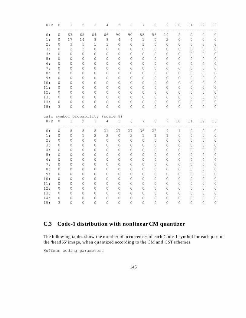
R\B 0 1 2 3 4 5 6 7 8 9 10 11 12 13------------------------------------------------------------------

0: 0 63 65 64 66 90 90 88 56 14 2 0 0 01: 0 17 14 8 8 4 4 1 0 2 0 0 0 02: 0 3 5 1 1 0 0 1 0 0 0 0 0 03: 0 2 3 0 0 0 0 0 0 0 0 0 0 04: 0 0 0 0 0 0 0 0 0 0 0 0 0 05: 0 0 0 0 0 0 0 0 0 0 0 0 0 06: 0 0 0 0 0 0 0 0 0 0 0 0 0 07: 0 0 0 0 0 0 0 0 0 0 0 0 0 08: 0 0 0 0 0 0 0 0 0 0 0 0 0 09: 0 0 0 0 0 0 0 0 0 0 0 0 0 010: 0 0 0 0 0 0 0 0 0 0 0 0 0 011: 0 0 0 0 0 0 0 0 0 0 0 0 0 012: 0 0 0 0 0 0 0 0 0 0 0 0 0 013: 0 0 0 0 0 0 0 0 0 0 0 0 0 014: 0 0 0 0 0 0 0 0 0 0 0 0 0 015: 3 0 0 0 0 0 0 0 0 0 0 0 0 0

calc symbol probability (scale 8)R\B 0 1 2 3 4 5 6 7 8 9 10 11 12 13

------------------------------------------------------------------0: 0 8 8 8 21 27 27 36 25 9 1 0 0 01: 0 0 1 2 2 0 2 1 1 1 0 0 0 02: 0 0 0 0 0 0 0 0 0 0 0 0 0 03: 0 0 0 0 0 0 0 0 0 0 0 0 0 04: 0 0 0 0 0 0 0 0 0 0 0 0 0 05: 0 0 0 0 0 0 0 0 0 0 0 0 0 06: 0 0 0 0 0 0 0 0 0 0 0 0 0 07: 0 0 0 0 0 0 0 0 0 0 0 0 0 08: 0 0 0 0 0 0 0 0 0 0 0 0 0 09: 0 0 0 0 0 0 0 0 0 0 0 0 0 010: 0 0 0 0 0 0 0 0 0 0 0 0 0 011: 0 0 0 0 0 0 0 0 0 0 0 0 0 012: 0 0 0 0 0 0 0 0 0 0 0 0 0 013: 0 0 0 0 0 0 0 0 0 0 0 0 0 014: 0 0 0 0 0 0 0 0 0 0 0 0 0 015: 3 0 0 0 0 0 0 0 0 0 0 0 0 0

C.3 Code-1 distribution with nonlinear CM quantizer

The following tables show the number of occurrences of each Code-1 symbol for each part ofthe ‘head55’ image, when quantized according to the CM and CST schemes.

Huffman coding parameters

146

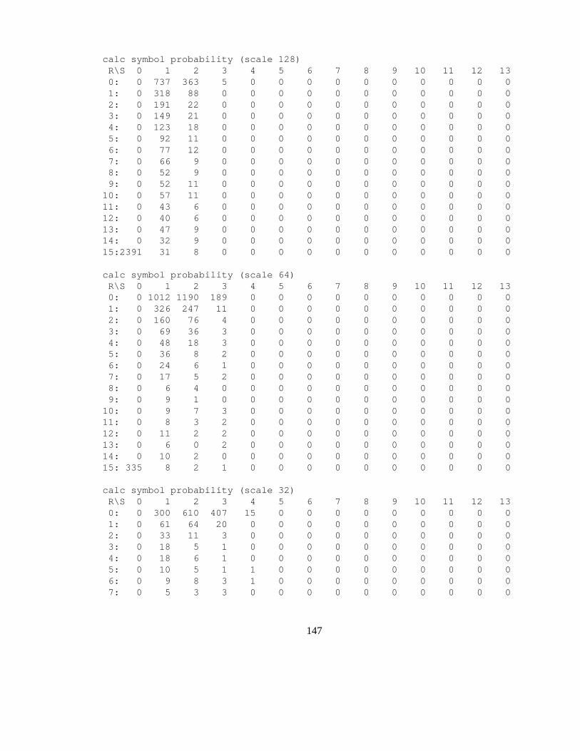
calc symbol probability (scale 128)R\S 0 1 2 3 4 5 6 7 8 9 10 11 12 130: 0 737 363 5 0 0 0 0 0 0 0 0 0 01: 0 318 88 0 0 0 0 0 0 0 0 0 0 02: 0 191 22 0 0 0 0 0 0 0 0 0 0 03: 0 149 21 0 0 0 0 0 0 0 0 0 0 04: 0 123 18 0 0 0 0 0 0 0 0 0 0 05: 0 92 11 0 0 0 0 0 0 0 0 0 0 06: 0 77 12 0 0 0 0 0 0 0 0 0 0 07: 0 66 9 0 0 0 0 0 0 0 0 0 0 08: 0 52 9 0 0 0 0 0 0 0 0 0 0 09: 0 52 11 0 0 0 0 0 0 0 0 0 0 010: 0 57 11 0 0 0 0 0 0 0 0 0 0 011: 0 43 6 0 0 0 0 0 0 0 0 0 0 012: 0 40 6 0 0 0 0 0 0 0 0 0 0 013: 0 47 9 0 0 0 0 0 0 0 0 0 0 014: 0 32 9 0 0 0 0 0 0 0 0 0 0 015:2391 31 8 0 0 0 0 0 0 0 0 0 0 0

calc symbol probability (scale 64)R\S 0 1 2 3 4 5 6 7 8 9 10 11 12 130: 0 1012 1190 189 0 0 0 0 0 0 0 0 0 01: 0 326 247 11 0 0 0 0 0 0 0 0 0 02: 0 160 76 4 0 0 0 0 0 0 0 0 0 03: 0 69 36 3 0 0 0 0 0 0 0 0 0 04: 0 48 18 3 0 0 0 0 0 0 0 0 0 05: 0 36 8 2 0 0 0 0 0 0 0 0 0 06: 0 24 6 1 0 0 0 0 0 0 0 0 0 07: 0 17 5 2 0 0 0 0 0 0 0 0 0 08: 0 6 4 0 0 0 0 0 0 0 0 0 0 09: 0 9 1 0 0 0 0 0 0 0 0 0 0 010: 0 9 7 3 0 0 0 0 0 0 0 0 0 011: 0 8 3 2 0 0 0 0 0 0 0 0 0 012: 0 11 2 2 0 0 0 0 0 0 0 0 0 013: 0 6 0 2 0 0 0 0 0 0 0 0 0 014: 0 10 2 0 0 0 0 0 0 0 0 0 0 015: 335 8 2 1 0 0 0 0 0 0 0 0 0 0

calc symbol probability (scale 32)R\S 0 1 2 3 4 5 6 7 8 9 10 11 12 130: 0 300 610 407 15 0 0 0 0 0 0 0 0 01: 0 61 64 20 0 0 0 0 0 0 0 0 0 02: 0 33 11 3 0 0 0 0 0 0 0 0 0 03: 0 18 5 1 0 0 0 0 0 0 0 0 0 04: 0 18 6 1 0 0 0 0 0 0 0 0 0 05: 0 10 5 1 1 0 0 0 0 0 0 0 0 06: 0 9 8 3 1 0 0 0 0 0 0 0 0 07: 0 5 3 3 0 0 0 0 0 0 0 0 0 0

147

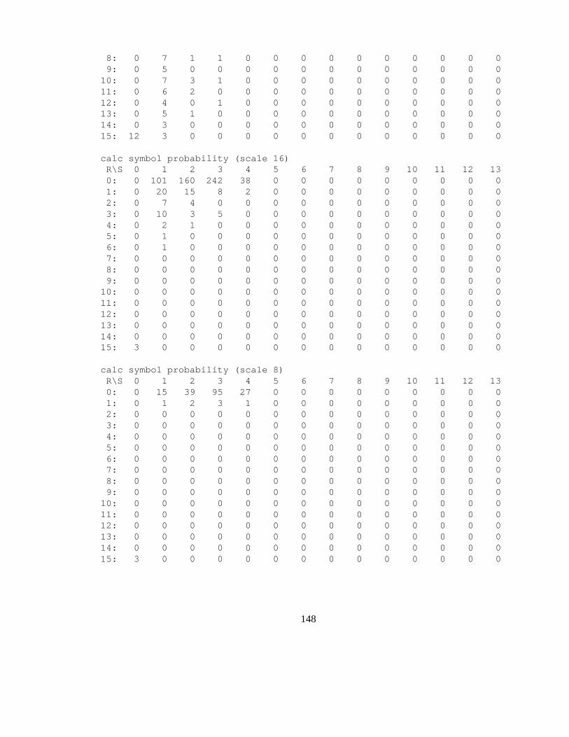
8: 0 7 1 1 0 0 0 0 0 0 0 0 0 09: 0 5 0 0 0 0 0 0 0 0 0 0 0 010: 0 7 3 1 0 0 0 0 0 0 0 0 0 011: 0 6 2 0 0 0 0 0 0 0 0 0 0 012: 0 4 0 1 0 0 0 0 0 0 0 0 0 013: 0 5 1 0 0 0 0 0 0 0 0 0 0 014: 0 3 0 0 0 0 0 0 0 0 0 0 0 015: 12 3 0 0 0 0 0 0 0 0 0 0 0 0

calc symbol probability (scale 16)R\S 0 1 2 3 4 5 6 7 8 9 10 11 12 130: 0 101 160 242 38 0 0 0 0 0 0 0 0 01: 0 20 15 8 2 0 0 0 0 0 0 0 0 02: 0 7 4 0 0 0 0 0 0 0 0 0 0 03: 0 10 3 5 0 0 0 0 0 0 0 0 0 04: 0 2 1 0 0 0 0 0 0 0 0 0 0 05: 0 1 0 0 0 0 0 0 0 0 0 0 0 06: 0 1 0 0 0 0 0 0 0 0 0 0 0 07: 0 0 0 0 0 0 0 0 0 0 0 0 0 08: 0 0 0 0 0 0 0 0 0 0 0 0 0 09: 0 0 0 0 0 0 0 0 0 0 0 0 0 010: 0 0 0 0 0 0 0 0 0 0 0 0 0 011: 0 0 0 0 0 0 0 0 0 0 0 0 0 012: 0 0 0 0 0 0 0 0 0 0 0 0 0 013: 0 0 0 0 0 0 0 0 0 0 0 0 0 014: 0 0 0 0 0 0 0 0 0 0 0 0 0 015: 3 0 0 0 0 0 0 0 0 0 0 0 0 0

calc symbol probability (scale 8)R\S 0 1 2 3 4 5 6 7 8 9 10 11 12 130: 0 15 39 95 27 0 0 0 0 0 0 0 0 01: 0 1 2 3 1 0 0 0 0 0 0 0 0 02: 0 0 0 0 0 0 0 0 0 0 0 0 0 03: 0 0 0 0 0 0 0 0 0 0 0 0 0 04: 0 0 0 0 0 0 0 0 0 0 0 0 0 05: 0 0 0 0 0 0 0 0 0 0 0 0 0 06: 0 0 0 0 0 0 0 0 0 0 0 0 0 07: 0 0 0 0 0 0 0 0 0 0 0 0 0 08: 0 0 0 0 0 0 0 0 0 0 0 0 0 09: 0 0 0 0 0 0 0 0 0 0 0 0 0 010: 0 0 0 0 0 0 0 0 0 0 0 0 0 011: 0 0 0 0 0 0 0 0 0 0 0 0 0 012: 0 0 0 0 0 0 0 0 0 0 0 0 0 013: 0 0 0 0 0 0 0 0 0 0 0 0 0 014: 0 0 0 0 0 0 0 0 0 0 0 0 0 015: 3 0 0 0 0 0 0 0 0 0 0 0 0 0

148

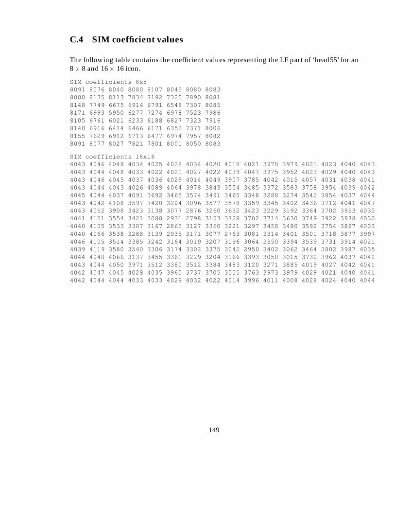
C.4 SIM coefficient values

The following table contains the coefficient values representing the LF part of ‘head55’ for an8� 8 and 16� 16 icon.

SIM coefficients 8x88091 8076 8040 8080 8107 8045 8080 80838080 8135 8113 7834 7192 7320 7890 80818148 7749 6675 6914 6791 6548 7307 80858171 6993 5950 6277 7274 6978 7523 79868105 6761 6021 6233 6188 6827 7323 79168140 6916 6414 6466 6171 6352 7371 80068155 7629 6912 6713 6477 6974 7957 80828091 8077 8027 7821 7801 8001 8050 8083

SIM coefficients 16x164043 4046 4048 4034 4025 4028 4034 4020 4018 4021 3978 3979 4021 4023 4040 40434043 4044 4048 4033 4022 4021 4027 4022 4039 4047 3975 3952 4023 4029 4040 40434043 4046 4045 4037 4036 4029 4014 4049 3907 3785 4042 4015 4057 4031 4038 40414043 4044 4043 4026 4089 4064 3978 3843 3554 3485 3372 3583 3758 3954 4039 40424045 4044 4037 4091 3692 3465 3574 3491 3465 3348 3288 3274 3542 3854 4037 40444043 4042 4108 3597 3420 3204 3096 3577 3578 3359 3345 3402 3436 3712 4041 40474043 4052 3908 3423 3138 3077 2876 3260 3632 3423 3229 3192 3364 3702 3953 40304041 4151 3554 3421 3088 2931 2798 3153 3728 3702 3714 3630 3749 3922 3938 40304040 4105 3533 3307 3167 2865 3127 3360 3221 3297 3458 3480 3592 3754 3897 40034040 4066 3538 3288 3139 2935 3171 3077 2763 3081 3314 3401 3501 3718 3877 39974046 4105 3514 3385 3242 3164 3019 3207 3096 3064 3350 3394 3539 3731 3914 40214039 4119 3580 3540 3306 3174 3302 3375 3042 2950 3402 3062 3464 3802 3987 40354044 4040 4066 3137 3455 3361 3229 3204 3166 3393 3058 3015 3730 3962 4037 40424043 4044 4050 3971 3512 3380 3512 3384 3483 3120 3271 3885 4019 4027 4042 40414042 4047 4045 4028 4035 3965 3737 3705 3555 3763 3973 3979 4029 4021 4040 40414042 4044 4044 4033 4033 4029 4032 4022 4014 3996 4011 4008 4028 4024 4040 4044

149

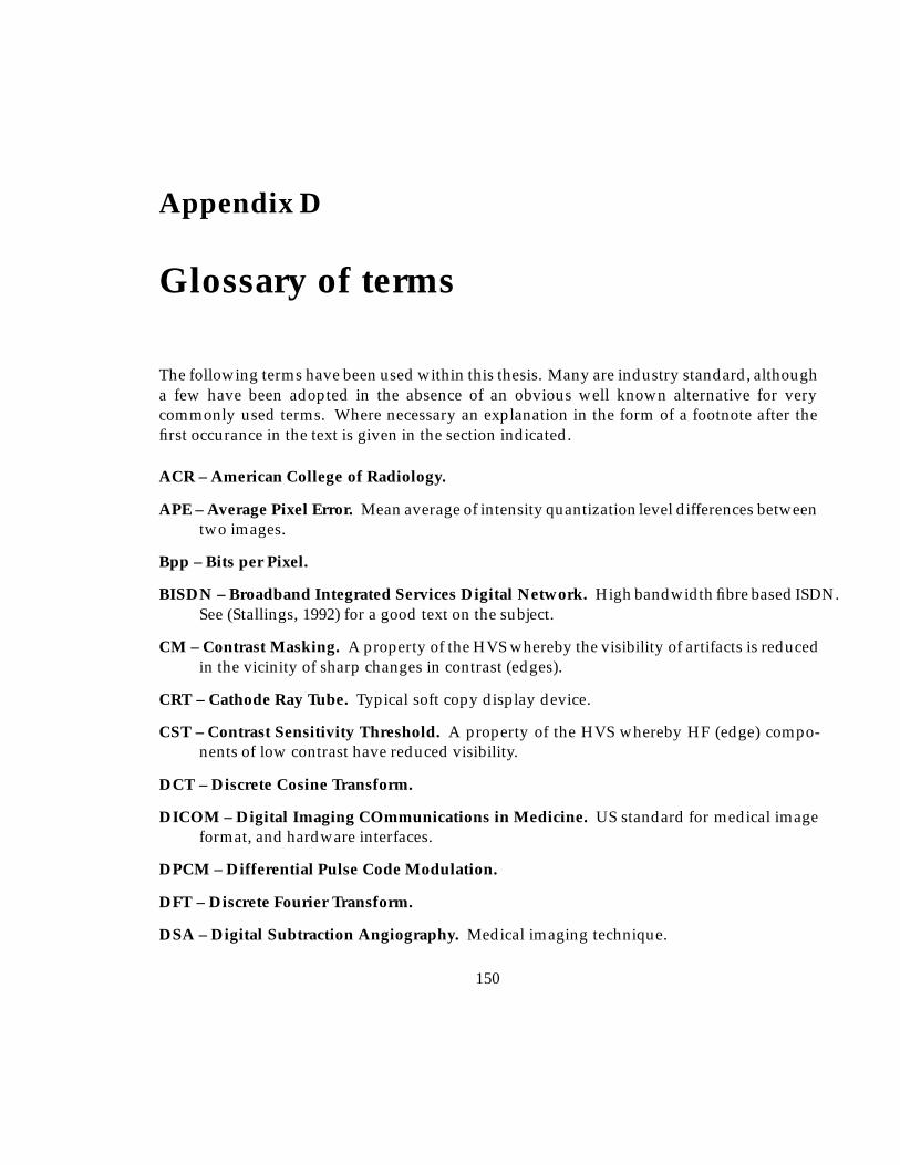
Appendix D

Glossary of terms

The following terms have been used within this thesis. Many are industry standard, althougha few have been adopted in the absence of an obvious well known alternative for verycommonly used terms. Where necessary an explanation in the form of a footnote after thefirst occurance in the text is given in the section indicated.

ACR – American College of Radiology.

APE – Average Pixel Error. Mean average of intensity quantization level differences betweentwo images.

Bpp – Bits per Pixel.

BISDN – Broadband Integrated Services Digital Network. High bandwidth fibre based ISDN.See (Stallings, 1992) for a good text on the subject.

CM – Contrast Masking. A property of the HVS whereby the visibility of artifacts is reducedin the vicinity of sharp changes in contrast (edges).

CRT – Cathode Ray Tube. Typical soft copy display device.

CST – Contrast Sensitivity Threshold. A property of the HVS whereby HF (edge) compo-nents of low contrast have reduced visibility.

DCT – Discrete Cosine Transform.

DICOM – Digital Imaging COmmunications in Medicine. US standard for medical imageformat, and hardware interfaces.

DPCM – Differential Pulse Code Modulation.

DFT – Discrete Fourier Transform.

DSA – Digital Subtraction Angiography. Medical imaging technique.

150

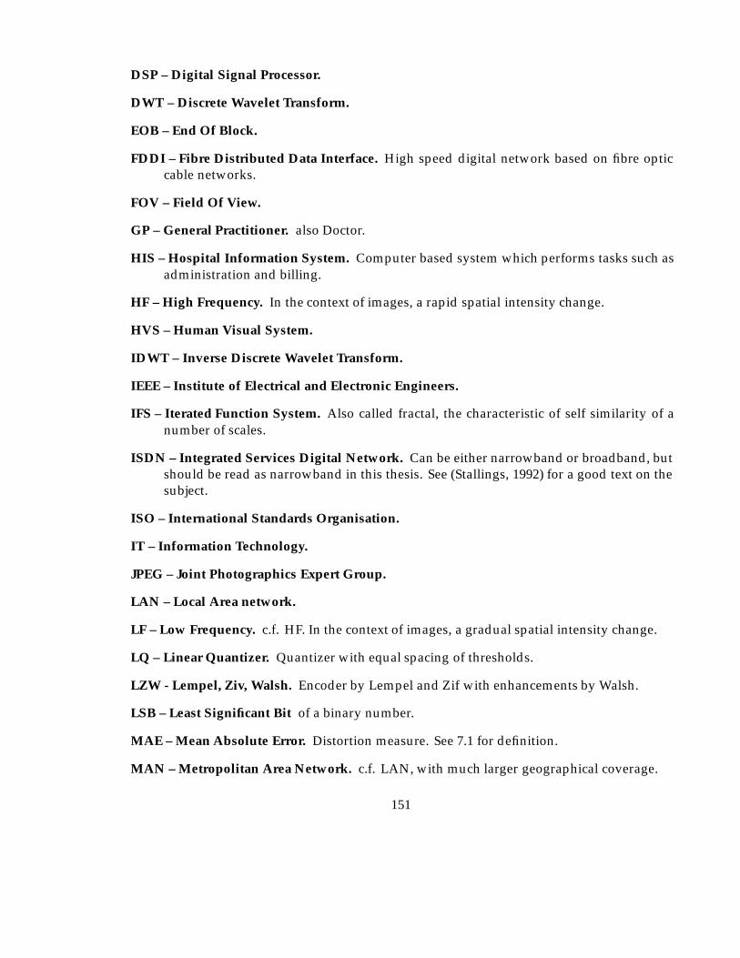
DSP – Digital Signal Processor.

DWT – Discrete Wavelet Transform.

EOB – End Of Block.

FDDI – Fibre Distributed Data Interface. High speed digital network based on fibre opticcable networks.

FOV – Field Of View.

GP – General Practitioner. also Doctor.

HIS – Hospital Information System. Computer based system which performs tasks such asadministration and billing.

HF – High Frequency. In the context of images, a rapid spatial intensity change.

HVS – Human Visual System.

IDWT – Inverse Discrete Wavelet Transform.

IEEE – Institute of Electrical and Electronic Engineers.

IFS – Iterated Function System. Also called fractal, the characteristic of self similarity of anumber of scales.

ISDN – Integrated Services Digital Network. Can be either narrowband or broadband, butshould be read as narrowband in this thesis. See (Stallings, 1992) for a good text on thesubject.

ISO – International Standards Organisation.

IT – Information Technology.

JPEG – Joint Photographics Expert Group.

LAN – Local Area network.

LF – Low Frequency. c.f. HF. In the context of images, a gradual spatial intensity change.

LQ – Linear Quantizer. Quantizer with equal spacing of thresholds.

LZW - Lempel, Ziv, Walsh. Encoder by Lempel and Zif with enhancements by Walsh.

LSB – Least Significant Bit of a binary number.

MAE – Mean Absolute Error. Distortion measure. See 7.1 for definition.

MAN – Metropolitan Area Network. c.f. LAN, with much larger geographical coverage.

151

MIDB – Medical Image DataBase.

MPE – Maximum Pixel Error. For images, the largest difference in intensity of any pixel.

MRI – Magnetic Resonance Imaging.

MSB – Most Significant Bit of a binary number.

MSE – Mean Square Error. Distortion measure. See 7.1 for definition.

NEMA – National Electrical Manufacturers Association.

N-ISDN – Narrowband ISDN. 2B+D channel digital communication channels. B channelsare 64K bit/s and D channel is 16K bit/s used for signalling.

NLQ – Non linear Quantizer. c.f. LQ. Quantizer with variable spacing of thresholds.

NMSE – Normalised Mean Square Error. Distortion measure. See 7.1 for definition.

PACS – Picture Archiving and Communication System.

PICON – Picture ICON. Similar to SIM.

QMF – Qradrature Mirror Filter. A pair of filters whose combined output represents thecomplete original signal.

RAID – Redundant Array of Internal Disks. Provides robust, reliable (large) storage.

RC – Repeat Code. Special code used when a runlength encoder finds a runlength too greatto be encoded. A RC is sent followed by the runlength code for the remainder of therunlength. Several RCs can be sent if necessary.

RIS – Radiological Information System. A computer system dedicated to handling infor-mation about radiological studies.

RISC – Reduced Instruction Set Computer.

ROC – Receiver Operating Characteristic. Method of determining the effects of systems orprocedures when dealing with tasks involving subjective analysis, by statistical means.

ROI – Region Of Interest. For images in this work. Some area of an image containing specificcharacteristics or anatomical detail of particular interest.

SIM – Spatial Information Model. A small (low resolution) version of a real image.

SNR – Signal to Noise Ratio, dB. Distortion measure. See 7.1 for definition.

TCP/IP – Transmission Control Protocol/ Internet Protocol.

UI – User Interface.

152

VLI – Variable Length Integer. An integer whose (positive) binary representation does notcontain any preceding zero bits.

VQ – Vector Quantization. Input symbols are mapped into a reduced set of symbols byapproximation to produce a compressed representation.

WAN – Wide Area Network. Larger geographical area than MAN, possibly worldwide com-prising many sub networks.

WIMPS – Windows, Icons, Menus, Pointer, System.

WORM – Write Once Read Many. Usually with respect to optical disk storage devices.

WT – Wavelet Transform.

ZRL – Zero Run Length. Representing a sequence of zeros in a data set by a count of thenumber of zeros in the sequence rather than the symbols themselves.

153

References

Aberle, D. R., et al. 1993. The effect of irreversible image compression on diagnostic accuracyin thoracic imaging. Investigative Radiology, 28(5), 398–403.

Alpert, B. K. 1992. Wavelets- A tutorial in theory and applications. Academic Press.

Apiki, S. 1991. Lossless data compression. Byte, March, 309–312.

Bakker, A. R., Didden, H., DeValk, J. P. J., & Baji, K. 1987. Traffic load on the image storagecomponent in a PACS. SPIE - Medical Imaging, 767, 824–829.

Barbosa, L. O., Karmouch, A., Georganas, N. D., & Goldberg, M. 1992. A multimediainterhospital communications system for medical consultants. IEEE Journal on SelectedAreas in Communications, 10(7), 1145–1157.

Barnes, G. T., Morin, R. L., & Staab, E. V. 1993. Computers for clinical practice and educationin radiology. Teleradiology: fundamental considerations and clinical applications.Radiographics, 13(3), 673–681.

Barnsley, M. 1990. Compressing pictures with fractals. Scientific American, March, 51–52.

Barnsley, M. F. 1988. Fractals Everywhere. 1st edn. New York: Academic Press.

Batnitzky, S. 1990. Teleradiology: an assessment. Radiology, 177(1), 11–17.

Bazis, Y., Forte, A., Gibaud, B., & Aubry, F. 1991. Storage and retrieval of medical image data,relationship to image processing and analysis. Pages 357–359 of: Huang, H. K., et al. (eds),Picture Archiving and Communications (PACS) in Medicine. London: Springer-Verlag, forNATO ASI Series, Vol. F74.

Beard, D., et al. 1987. A prototype single-screen PACS console development using humancomputer interaction techniques. SPIE - Medical Imaging, 767, 646–653.

Beaumont, J. M. 1991. Image data compression using fractal techniques. BT Technology Journal,9(4), 93–109.

Bijl, K., Koens, M. L., Bakker, A. R., & deValk, J. P. J. 1987. Medical PACS and HIS: integrationneeded ! SPIE - Medical Imaging, 767, 765–769.

154

Binkhuysen, F. H. B. 1992. Impact of PACS on radiologists’ daily work in western countries.IEEE Journal on Selected Areas in Communications, 10(7), 1158–1160.

Blume, H., & Kamiya, K. 1987. Auto-ranging and normalisation versus histogrammodifications for automatic image processing of digital radiographs. SPIE, 767, 371–383.

Boom, D. C. 1987. Image processing on the IBM PC. SPIE - Medical Imaging, 767, 663–669.

Brauer, G. W. 1992. Telehealth: the delayed revolution in health care. Medical Progress ThroughTechnology, 18, 151–163.

Bridgood, W. D., & S.C.Horii. 1992. PACS mini refresher course (introduction to the ACR-NEMA dicom standard. Radiographics, 12(2), 345–354.

Bridgood, W. D., & Staab, E. V. 1992. Understanding and using teleradiology. Seminars inUltrasound, CT and MRI, 13(2), 102–112.

Brink, J. V., Cywinski, J., & Szerlag, C. T. 1987. Cost analysis of present methods of imagemanagement. SPIE - Medical Imaging, 767, 758–764.

Bruce, K. T. 1987. Expandable image compression system - A modular approach. SPIE, 767,286–289.

Cetin, A. E. 1991. Subband coding of DSA images. Pages 361–363 of: Huang, H. K., et al. (eds),Picture Archiving and Communications (PACS) in Medicine. London: Springer-Verlag, forNATO ASI Series, Vol. F74.

Chen, J., Itoh, S., & Hashimoto, T. 1993. Scalar quantization noise analysis and optimalbit allocation for wavelet pyramid image encoding. IEICE Trans. Fundamentals, E76(9),1502–1504.

Chimiak, W. J. 1992. The digital radiology environment. IEEE Journal on Selected Areas inCommunications, 10(7), 1133–1144.

Chipman, K., Holzworth, P., Loop, J., ransom, N., Spears, D., & Thompson, B. 1992. Medicalapplications in a B-ISDN field trial. IEEE Journal on Selected Areas in Communications,10(7), 1173–1187.

Cho, P. S., et al. 1987. A PACS module for the coronary care unit. SPIE - Medical Imaging, 767,577–583.

Cho, P. S., Chan, K. K., & Ho, B. K. T. 1991a. Data storage and compression. Pages 71–82of: Huang, H. K., et al. (eds), Picture Archiving and Communications (PACS) in Medicine.London: Springer-Verlag, for NATO ASI Series, Vol. F74.

Cho, P. S., Chan, K. K., & Ho, B. K. T. 1991b. Distributed acquisition of digital images in a ruralsetting. Pages 427–429 of: Huang, H. K., et al. (eds), Picture Archiving and Communications(PACS) in Medicine. London: Springer-Verlag, for NATO ASI Series, Vol. F74.

155

Cody, M. A. 1992. The fast wavelet transform. Dr Dobbs Journal, April, 16–28.

Coifman, R. R., & Wickerhauser, M. V. 1992. Entropy-based algorithms for best basis selection.IEEE Transactions on Information Theory, 38(2), 713–718.

Cox, J. R., et al. 1992. Considerations in moving electronic radiography into routine use. IEEEJournal on Selected Areas in Communications, 10(7), 1108–1120.

Curtis, P. T., Gayler, B. W., Gitlin, J. N., & Harrington, M. B. 1983. Radiology. Proc SPIE, 149,415–481.

Dallas, W. J., & Roehrig, H. 1987. A dynamically programmed computer algorithm forassisting the radiologist in locating vessels. SPIE - Medical Imaging, 767, 462–470.

Dallas, W. J., et al. 1987. A prototype totally digital radiology department: conception andinitiation. SPIE - Medical Imaging, 767, 700–707.

Daubechies, I. 1988. Orthonormal bases of compactly supported wavelets. Commun. PureAppl. Math, 41, 909–996.

DeVore, R. A., et al. 1992. Image compression through transform coding. IEEE Transactions onInformation Theory, 38(2), 719–746.

D’Silva, V., H.Perros, & Stockbridge, C. 1988. A Simulation model of a picture archival andcommunications system. SPIE - Medical Imaging II, 914, 940–946.

Dwyer, S. J. 1992. PACS mini refresher course (Wide area network strategies for teleradiologysystems. Radiographics, 12(3), 567–576.

Dwyer, S. J., et al. 1992. Teleradiology using switched dialup networks. IEEE Journal on SelectedAreas in Communications, 10(7), 1161–1172.

Eljamel, M. S., & Nixon, T. 1992. The use of a computer based image link system to assist interhospital referrals. British Journal of Neurosurgery, 6, 559–562.

Elnahas, S. E., et al. 1986. Progressive coding and transmission of digital diagnostic pictures.IEEE Trans. on medical imaging., MI-5(2), 73–83.

Farman, A. J., Farag, A. A., & Yeap, P. Y. 1992. Expediating prior approval and containingthird-party costs for dental care. Annals New York Academy Sciences, 670(December),269–276.

Fiske, R. A., Valentino, D. J., & Huang, H. K. 1987. The effect of digital image display formaton perceived image quality. SPIE - Medical Imaging, 767, 631–638.

Franken, E. A. 1992. Teleradiology for consultation between practitioners and radiologists.Annals New York Academy Sciences, 670(December), 277–280.

156

Frost, M., & Staab, E. V. 1989. Special series: digital radiology. displays contrast and spatialrequirements. Investigative Radiology, 24(2), 95–98.

Fua, P., & Leclerc, Y. G. 1990. Model driven edge detection. Machine Vision and Applications, 3,45–56.

Giger, M. L., et al. 1993. An ‘intelligent’ workstation for computer aided diagnosis.Radiographics, 13(3), 647–656.

Glenn, W. E. 1993. Digital image compression based on visual perception and Scene Properties.SMPTE Journal, May, 392–397.

Goldberg, M. A., Rosenthal, D. J., Chew, F. S., Blickman, J. G., Miller, S. W., & Mueller,P. R. 1993. New high resolution teleradiology system: prospective study of diagnosticaccuracy in 685 transmitted clinical cases. Radiology, 186(2), 429–434.

Griffin, L. D., Colchester, A. C. F., & Robinson, G. P. 1990. Scale and segmentation of grey-levelimages using maximum gradient paths. Tech. rept. Dept. of Neurology, Guy’s Hospital,London.

Harlow, C. A., & Eisenbeis, S. A. 1973. The analysis of radiographic images. IEEE Trans. onComputers, C-22(7), 678–689.

Herron, J. M., et al. 1987. High resolution work station for evaluation of diagnostic efficacy.SPIE - Medical Imaging, 767, 670–673.

H.Kangarloo. 1991. PACS-clinical experience at UCLA. Pages 189–194 of: NATO ASI Series F- PACS in Medicine. London: Springer-Verlag, for NATO.

Honeyman, J. C. 1991. Teleradiology and network strategies. Pages 95–111 of: NATO ASISeries F - PACS in Medicine. London: Springer-Verlag, for NATO.

Horii, S. C. 1987. Peak data rates for image generation: Implications for PACS. SPIE - MedicalImaging, 767, 681–687.

Horii, S. C., & Bridgood, W. D. 1992. PACS mini refresher course (network and ACR-NEMAprotocols). Radiographics, 12(3), 537–548.

Huang, H. K. 1991. Image storage, transmission and manipulation. Minimally Invasive Therapy,1, 85–92.

Huang, H. K., Wong, W. K., l. Lou, S., & Stewart, B. K. 1992. Architecture of a comprehensiveradiologic imaging network. IEEE Journal on Selected Areas in Communications, 10(7),1188–1202.

Irie, G. 1991. Clinical Experience. 16 months of HU-PACS. Pages 183–188 of: Huang, H. K., et al.(eds), Picture Archiving and Communications (PACS) in Medicine. London: Springer-Verlag,for NATO ASI Series, Vol. F74.

157

Jacquin, A. E. 1990. A novel fractal block-coding technique for digital images. Pages 2225–2228of: IEEE Int Conf. on Acoustics, Speech, and Signal Processing. -: IEEE, for IEEE.

Johnson, R. E., et al. 1987. How to evaluate a medical imaging display workstation. SPIE -Medical Imaging, 767, 616–621.

Kagetsu, N. J., & Ablow, R. C. 1992. Teleradiology for the emergency room. Annals New YorkAcademy Sciences, 670(December), 293–297.

Kajiwara, K. 1992. Overview of JPEG: Is it acceptable in medical fields ? Pages 762–767 of:Medinfo 92. -: Elsevier Science Publishers B.V., for IMIA.

Kergosien, Y. L. 1991. Generic sign systems in medical imaging. IEEE Computer Graphics andapplications, September, 46–65.

Komori, M., et al. 1987. Pilot PACS with on-line communication between an image workstationand CT scanners in a clinical environment. SPIE - Medical Imaging, 767, 744–751.

Kositpaiboon, R., et al. 1989. Packetized radiographic image transfers over local area networksfor diagnosis and conferencing. IEEE Journal on Selected Areas in Communications, 7(5),842–856.

Lear, J. L., et al. 1989. Ultra highspeed teleradiology with ISDN technology. Radiology, 171(3),862–863.

Lee, H., et al. 1993. A new method for computed tomography image compression usingadjacent slice data. Investigative Radiology, 28(8), 678–685.

Ligier, Y., Funk, M., Ratib, O., Girard, C., Perrier, R., & Snydr-Michal, J. 1992. Object orienteddesign of a portable platform for medical image manipulation. Pages 26–32 of: sdfg (ed),Medinfo 92. -: Elsevier Science Publishers B.V., for IMIA.

Lisse, E. W. 1992. An overview of networking for physicians and problems of networkconsulting in remote areas. Annals New York Academy Sciences, 670(December), 19–28.

London, J. W., & Morton, D. E. 1992. The integration of text, graphics, and radiographicimages on X-terminal clinical workstations. Pages 41–46 of: Medinfo 92. -: ElsevierScience Publishers B.V., for IMIA.

Mallat, S. G. 1989. A Theory for multiresolution signal decomposition: the wavelet transform.IEEE Transactions on Pattern Analysis and Machine Intelligence, 11(7), 674–693.

Manikopoulos, C., Sun, H., & Antoniou, G. 1989. Image coding with finite state vectorquantization utilising extrapolation selection. IEEE, CH2682-3/89/0000-0575, 575–579.

Mankovich, N. J. 1987. An image database structure for pediatric radiology. SPIE - MedicalImaging, 767, 564.

158

Manninen, H., Partanen, K., Lehtovirta, J., Matsi, P., & Soimakallio, S. 1992. Image processingin digital chest radiography: effect on diagnostic efficacy. European Journal of Radiology,14, 164–168.

Markivee, C. R. 1989. Diagnostic accuracy of a teleradiology image transmission system. M.D. Computing, 6(2), 88–93.

Marsi, S., & Carrelo, S. 1992. Parallel structure based on neural networks for imagecompression. Electronics Letters, 28(12), 1152–1153.

Matthews, R. 1991. PACS and PACS related research in Belgium. In: NATO ASI Series F -PACS in Medicine. London: Springer-Verlag, for NATO.

McNeill, K. M., & Fisher, H. D. 1987. A model for radiologic workstation user interface design.SPIE - Medical Imaging, 767, 713–716.

Minato, K., Komori, M., Nakano, Y., & Takahashi, T. 1992. Decentralized PAC system a KyotoUniversity Hospital. Pages 270–274 of: Medinfo 92. London: Elsevier Science PublishersB.V., for IMIA.

Mongatti, G., et al. 1992. Progressive image transmission by content driven laplacian pyramidencoding. IEE proceedings -I, 139(5), 495–500.

Nill, N. B., & Bouzas, B. H. 1992. Objective image quality measure derived from digital imagepower spectra. Optical Engineering, 31(4), 813–825.

Ohta, M., Yano, M., & Nishitani, T. 1992. Wavelet picture coding with transform codingapproach. IEICE Transactions Fundamentals, E75-A(7), 776–785.

Okabe, T. 1991. PACS and PACS related research in Japan. Pages 289–293 of: Huang, H. K., et al.(eds), Picture Archiving and Communications (PACS) in Medicine. London: Springer-Verlag,for NATO ASI Series, Vol. F74.

Okabe, T., Satoh, K., & Kabata, S. 1991. Introduction to Hitachi PACS. Pages 241–245 of: Huang,H. K., et al. (eds), Picture Archiving and Communications (PACS) in Medicine. London:Springer-Verlag, for NATO ASI Series, Vol. F74.

Ozeki, T., et al. 1987. Investigation and analysis of the requirements for a picture archivingand communications system at the university of Arizona Health Sciences Center. SPIE -Medical Imaging, 767, 733–741.

Parikh, V. N., & Baraniecki, A. Z. 1993. Comparison of RISC and DSP processors for a transformdomain implementation of the discrete wavelet transform. Journal of MicrocomputerApplications, 16(1), 19–31.

Popescu, D. C., & Yan, H. 1993. MR image compression using iterated function systems.Magnetic Resonance Imaging, 11, 727–732.

159

Press, W. H. 1991. Wavelet transforms. Tech. rept. 3184. Harvard-Smithsonian Center forAstrophysics.

Ratib, O., et al. 1991a. Digital imaging network systems in the U.S. military: Past, Present,Future. Pages 207–212 of: Huang, H. K., et al. (eds), Picture Archiving and Communications(PACS) in Medicine. London: Springer-Verlag, for NATO ASI Series, Vol. F74.

Ratib, O., et al. 1991b. PACS Workstation: user interface design. Pages 57–61 of: Huang,H. K., et al. (eds), Picture Archiving and Communications (PACS) in Medicine. London:Springer-Verlag, for NATO ASI Series, Vol. F74.

Rioul, O., & Duhamel, P. 1992. Fast algorithms for discrete and continuous wavelet transforms.IEEE Transactions on information Theory, 38(2), 569–586.

Romaniuk, S. G., Namuduri, K. R., & Ranganathan, N. 1993 (January). A feature based heuristicalgorithm for lossless image compression. Tech. rept. TRC1/93. Dept. of information systemsand computer science, National University of Singapore.

Schilling, R. B. 1993. Computers for clinical practice and education in radiology. Teleradiology,information transfer and implications for diagnostic imaging in the 1990s. Radiographics,13(3), 686–686.

Schuttenbeld, H. W., & Romeny, B. M. 1987. Design of a user interface for a PACS viewingstation. SPIE - Medical Imaging, 767, 844–852.

Scott, W. W., et al. 1993. Subtle orthopedic fractures: teleradiology workstation versus filminterpretation. Musculoskeletal radiology, 187(3), 811–815.

Seeley, G. W., McNeill, K. M., et al. 1987a. An overview of picture archiving andcommunications systems related psychophysical research in the University of ArizonaRadiology Department. SPIE - Medical Imaging, 767, 726.

Seeley, G. W., et al. 1987b. The use of psychophysics as a system design: comparison of filmscreen to an electronic review console. SPIE - Medical Imaging, 767, 639–643.

Sezan, M. I., Yip, K. L., & Daly, S. J. 1987. An investigation of the effects of uniform perceptualquantization in the context of digital radiography. SPIE - Medical Imaging, 767, 622–630.

Siebert, J. E., & Rossenbaum, T. L. 1986. Experience and insights with a metropolitan areamedical imaging broadband network. SPIE Proc. Int. Soc. Opt. Eng., 626, 1986.

Smith, B. C., & Rowe, L. A. 1993. Algorithms for manipulating compressed images. IEEEComputer Graphics and Applications, September, 34–43.

Snooke, N. A. 1992 (May). The ISDN as a platform for teleradiology. In: European ISDNuser Forum IV Plenary Meeting. EIUF, CEC, DG XIII, 200, rue de la Loi, B-1049 Brussels,Belgium.

160

Soryani, M., & Clarke, R. J. 1992. Segmented coding of digital image sequences. IEEProceedings-I, 139(2), 212–218.

Stallings, W. 1992. ISDN and Broadband ISDN. 2nd edn. Maxwell MacMillan.

Stevenson, D., Beard, D., & Parish, D. 1989. Medical image communications as an applicationfor broadband ISDN. SPIE, 1179, 584–594.

Stewart, B. K., & Dwyer, S. J. 1992. Special section: digital radiology. Prediction ofteleradiology throughput by discrete event driven block-oriented network simulation.Investigative Radiology, 28(2), 162–168.

Sui, T., & Rosenfeld, D. 1987. A PC based medical imaging workstation. SPIE - MedicalImaging, 767, 654–658.

Sun, H., & Goldberg, M. 1987. Medical image sequence coding using vector quantization.SPIE, 767, 281–285.

Taira, R. K. 1987. Operational characteristics of pediatric radiology image display stations.SPIE - Medical Imaging, 767, 571–576.

Tan, K. H., & Ghanbari, M. 1992. Compact image coding using two dimensional DCT pyramid.Electronics Letters, 28(8), 791–792.

Tischer, P. E., Worley, R. T., Meader, A. J., & Goodwin, M. 1993. Context-based lossless imagecompression. The Computer Journal, 36(1), 68–77.

Tobes, M. C. 1987. Teleradiology operations within a PACS environment. SPIE - MedicalImaging, 767, 849–851.

Todd, S., Langdon, G., & Rissanen, J. 1985. Parameter reduction and context selection forcompression of greyscale images. IBM Journal Research and Development, 29(2), 188–193.

Treves, S. T., et al. 1992. Multimedia communications in medical imaging. IEEE Journal onSelected Areas in Communications, 10(7), 1121–1132.

VanAken, I. W., Reijns, G. L., de Valk, J. P. J., & Nijhof, J. A. M. 1987. Compressed medicalimages and enhanced fault detection within an ACR-NEMA compatible picture archivingand communications system. SPIE - Medical Imaging, 767, 290–296.

Vercillo, R., et al. 1987. Digital image review console. SPIE - Medical Imaging, 767, 708–712.

Waite, J. B., & Welsh, W. J. 1990. Head boundary location using snakes. British telecomtechnology journal, 8(3), 127–135.

Wallace, G. K. 1991. The JPEG still picture compression standard. Communications of the ACM,34(4), 31–44.

161

Wallace, G. K. 1992. The JPEG Still picture image compression standard. IEEE Transactions onConsumer Electronics, 38(1), 18–34.

Wang, L., & Goldberg, M. 1987. Progressive image transmission using vector quantization onimages in pyramid form. IEEE, 37, 1339–1349.

Wang, Y., et al. 1987. A summary of compatibility of the ACR-NEMA imaging andcommunications standard. SPIE - Medical Imaging, 767, 819–822.

Watson, A. B. 1987. Efficiency of a human model image code. Journal Optical Society of America,4(12), 2401–2416.

Webber, M. M., et al. 1973. Telecommunication of images in the practice diagnostic radiology.Diagnostic Radiology, 109(October), 71–74.

Wickerhauser, M. V. 1993. Picture compression by best basis sub-band coding. Tech. rept. NumericalAlgorithms Research Group, Yale University.

Willis, C. E. 1991. Distributed acquisition of digital images in a rural setting. Pages 427–429of: Huang, H. K., et al. (eds), Picture Archiving and Communications (PACS) in Medicine.London: Springer-Verlag, for NATO ASI Series, Vol. F74.

Woods, J. W. 1986. Subband coding of images. IEEE Transactions on Acoustics, Speech, andSignal Processing, 34(5), 1278–1288.

Wu, X. 1992. Image coding by adaptive tree structured segmentation. IEEE Transactions oninformation Theory, 38(6), 1755–1767.

Yamamoto, L. G., Dimauro, R., & Long, D. C. 1993a. Personal computer teleradiology:comparing image quality of lateral cervical spine radiographs with conventionalteleradiology. American Journal of Emergency Medicine, 11(4), 384–389.

Yamamoto, L. G., et al. 1993b. Scanned computed tomography image transmission by modem.American Journal of Emergency Medicine, 10(3), 226–229.

Yoshino, M. T., et al. 1992. Diagnostic performance of teleradiology in cervical spine fracturedetection. Investigative Radiology, 27(January), 55–59.

162