Embed Size (px)
Citation preview
Medical Image Segmentation‐‐‐‐
Module 1
Hervé Delingette MASTER2 MVA
2017/18
1
Overview
• Introduction to image segmentation•Thresholding and Filtering•Mathematical Morphology
4
Segmentation
1. Introduction
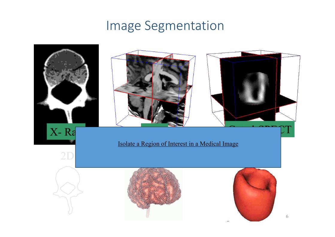
Image Segmentation
4D (3D+T)
Gated-SPECT
2D 3D
X- Ray MRIIsolate a Region of Interest in a Medical Image
6
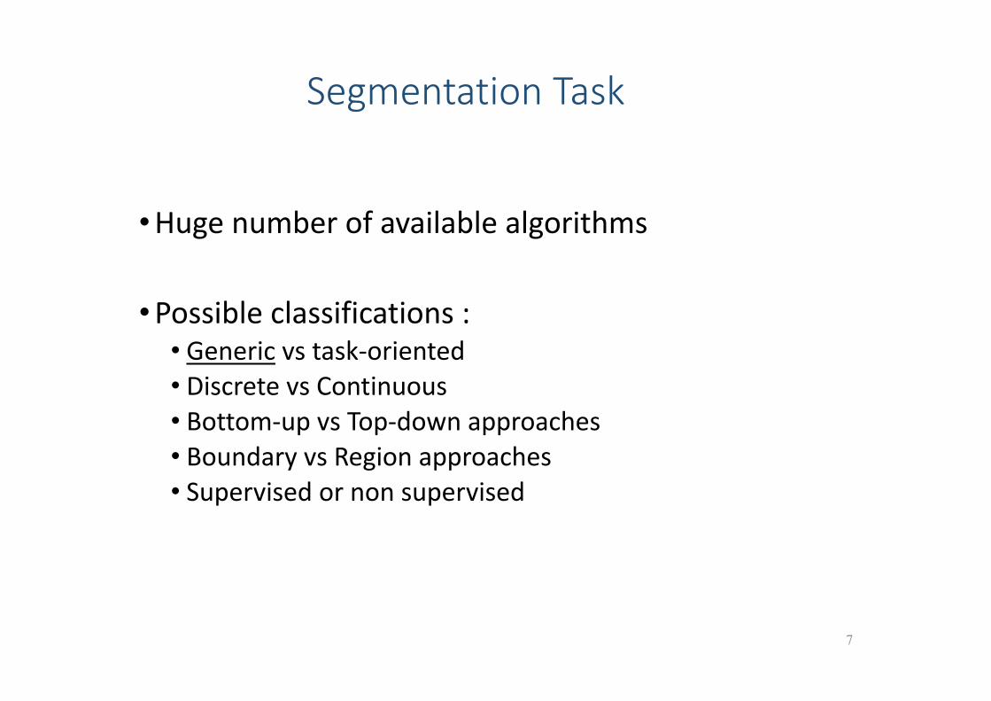
Segmentation Task
•Huge number of available algorithms
•Possible classifications :• Generic vs task‐oriented• Discrete vs Continuous• Bottom‐up vs Top‐down approaches • Boundary vs Region approaches• Supervised or non supervised
7
Discrete vs Continuous Image Representation
8
Discrete Image Representation
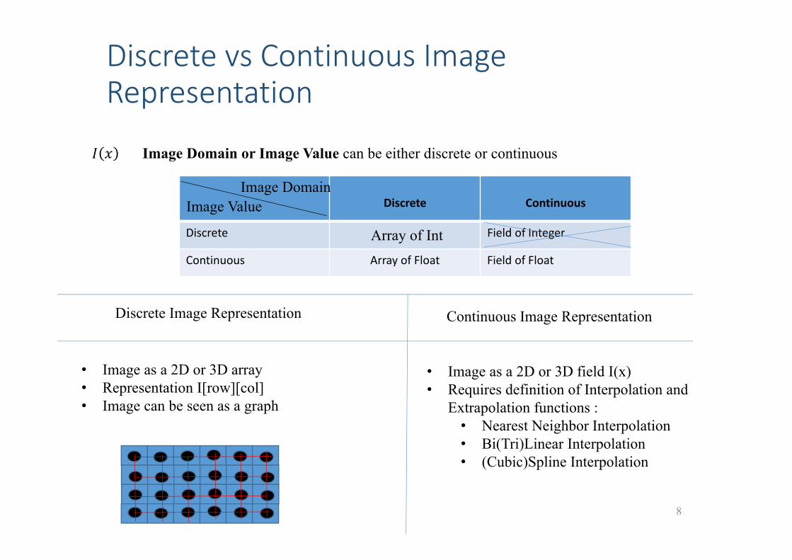
Image Domain or Image Value can be either discrete or continuous
Discrete Continuous
Discrete Field of Integer
Continuous Array of Float Field of Float
Image DomainImage Value
Array of Int
• Image as a 2D or 3D array• Representation I[row][col]• Image can be seen as a graph
• Image as a 2D or 3D field I(x)• Requires definition of Interpolation and
Extrapolation functions :• Nearest Neighbor Interpolation• Bi(Tri)Linear Interpolation• (Cubic)Spline Interpolation
Continuous Image Representation
Discrete vs Continuous Image Segmentations
9
Discrete Image Representation Continuous Image Representation
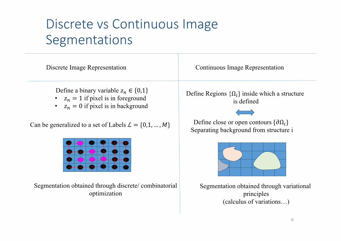
Define a binary variable ∈ 0,1• 1 if pixel is in foreground• 0 if pixel is in background
Can be generalized to a set of Labels 0,1,… ,
Segmentation obtained through discrete/ combinatorial optimization
Define Regions {Ω inside which a structure is defined
Define close or open contours ΩSeparating background from structure i
Segmentation obtained through variationalprinciples
(calculus of variations…)
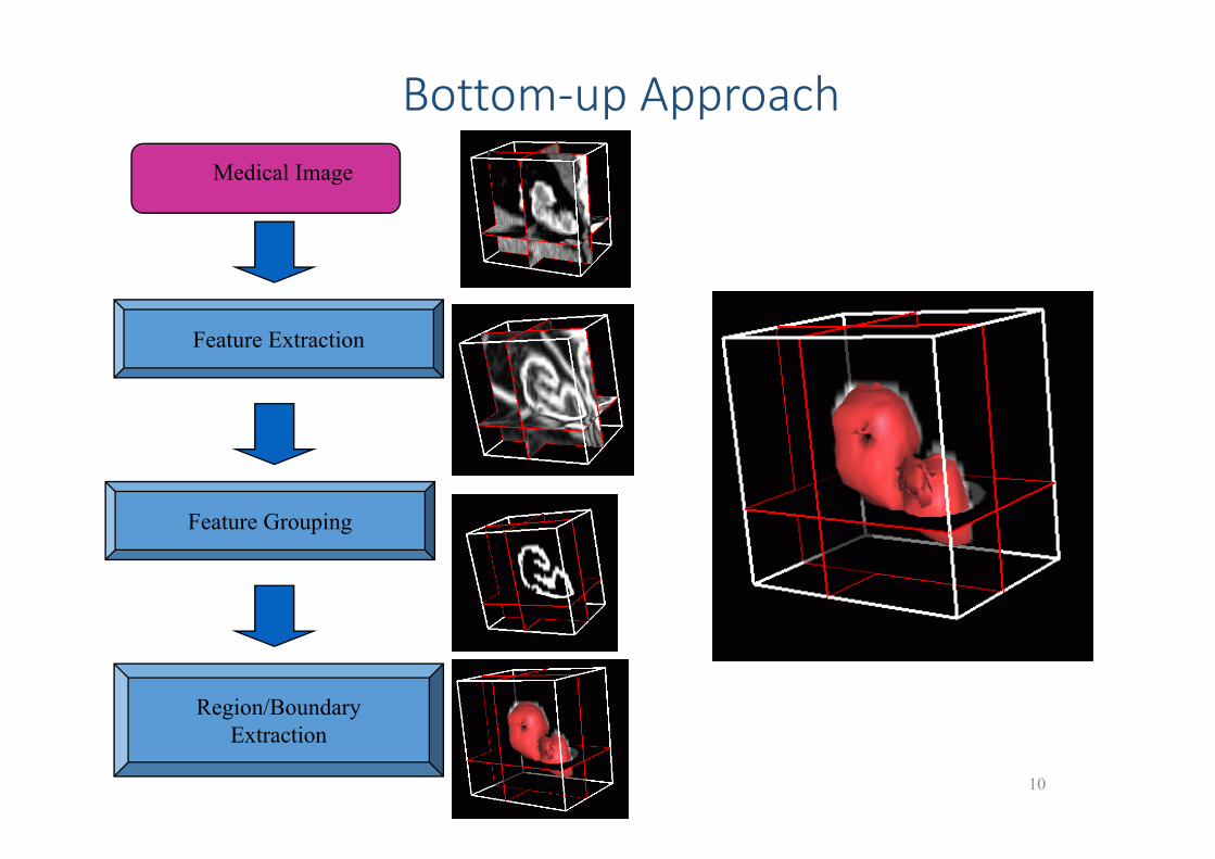
Bottom‐up ApproachMedical Image
Feature Extraction
Feature Grouping
Region/BoundaryExtraction
10
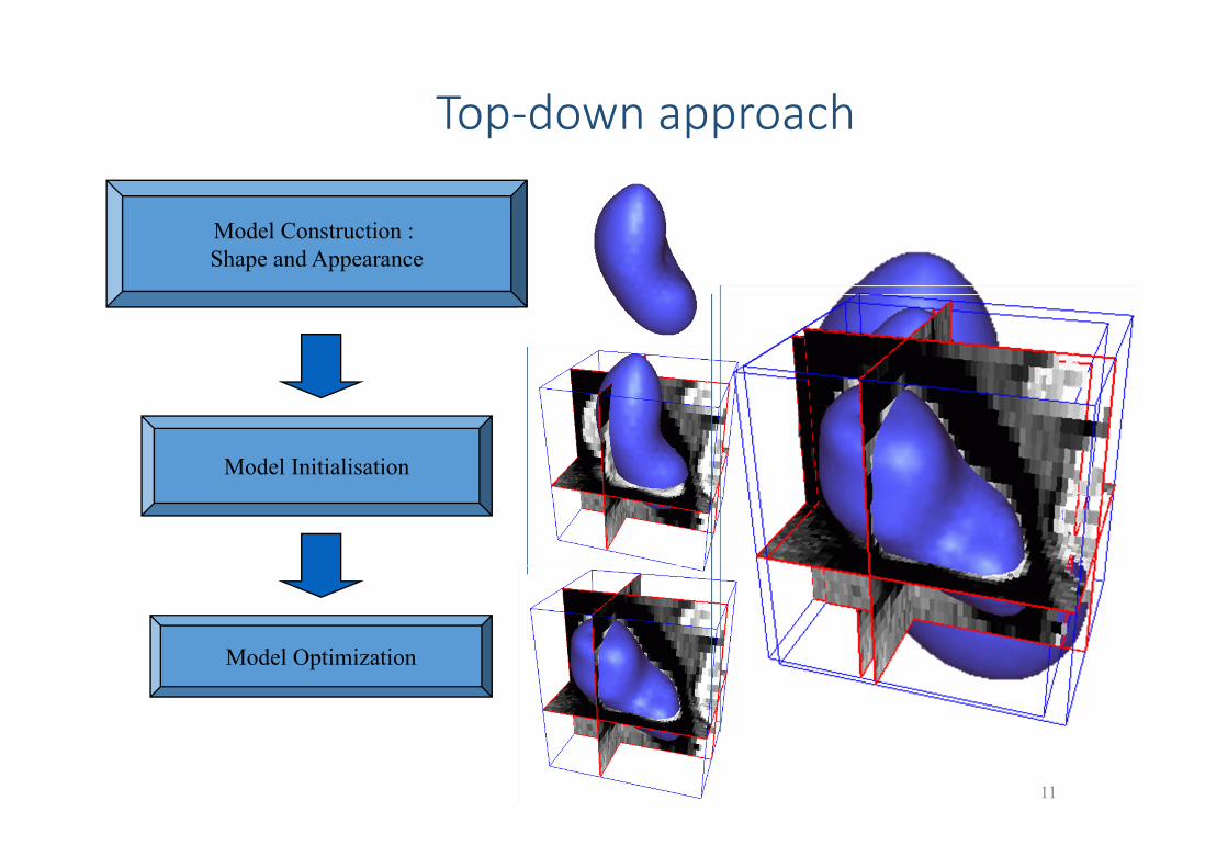
Top‐down approach
Model Construction : Shape and Appearance
Model Initialisation
Model Optimization
11
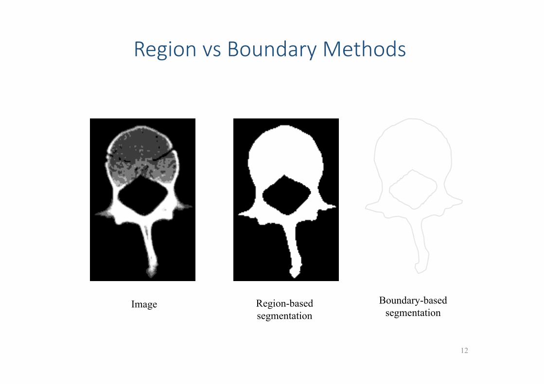
Region vs Boundary Methods
Region-basedsegmentation
Boundary-basedsegmentation
Image
12
Supervised vs Unsupervised Image Segmentation
•Supervised Image Segmentation Problems:• Several examples of image segmentations are available• Methods : machine learning, multi‐atlas registration• Very costly to produce annotated data
•Unsupervised Image Segmentation Problems :• No examples are available• Models of image content and shape are used to produce image segmentation
•Weakly supervised Segmentation Problems :• Only partial labels are available
13
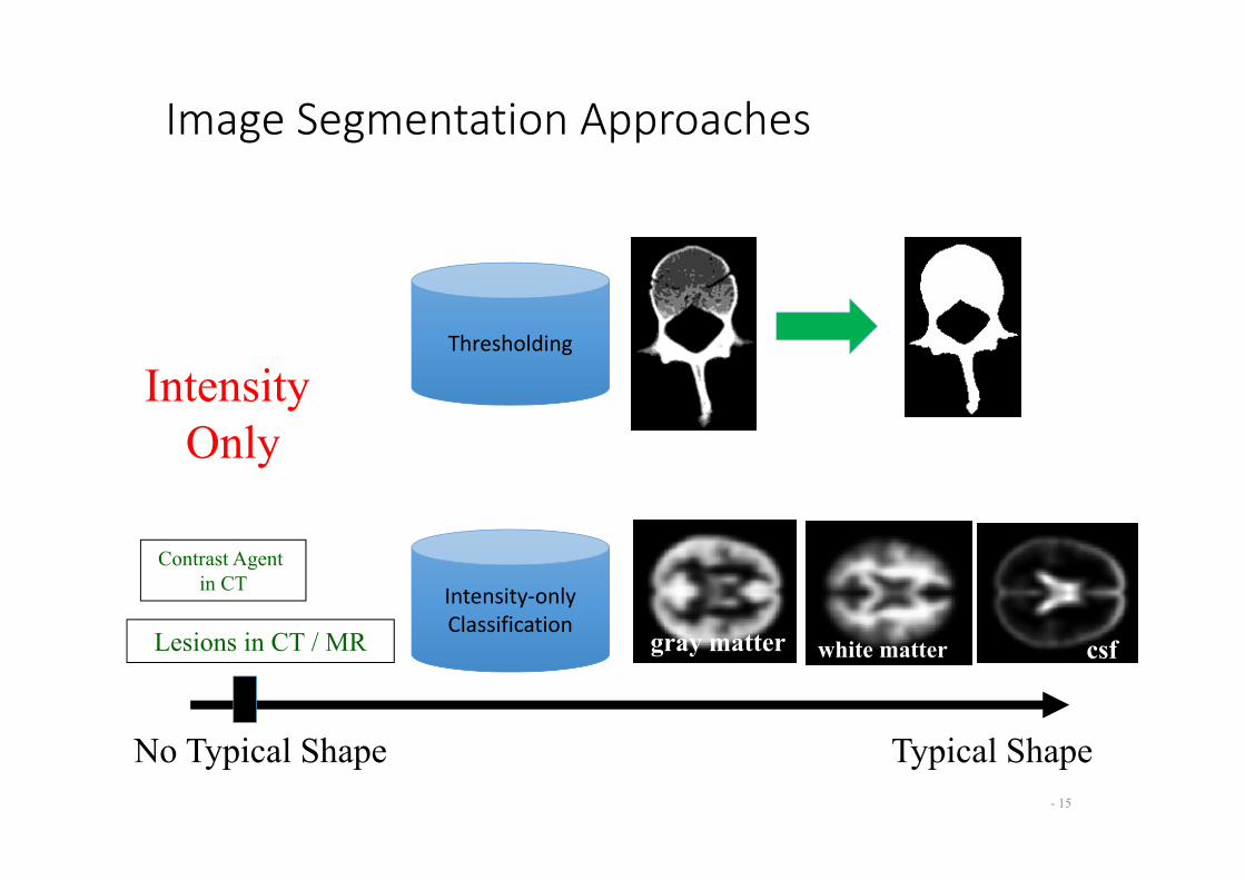
Image Segmentation Approaches
- 15
24/10/2017 15
No Typical Shape Typical Shape
Lesions in CT / MR
Contrast Agent in CT
Thresholding
Intensity‐onlyClassification
Intensity Only
gray matter white matter csf
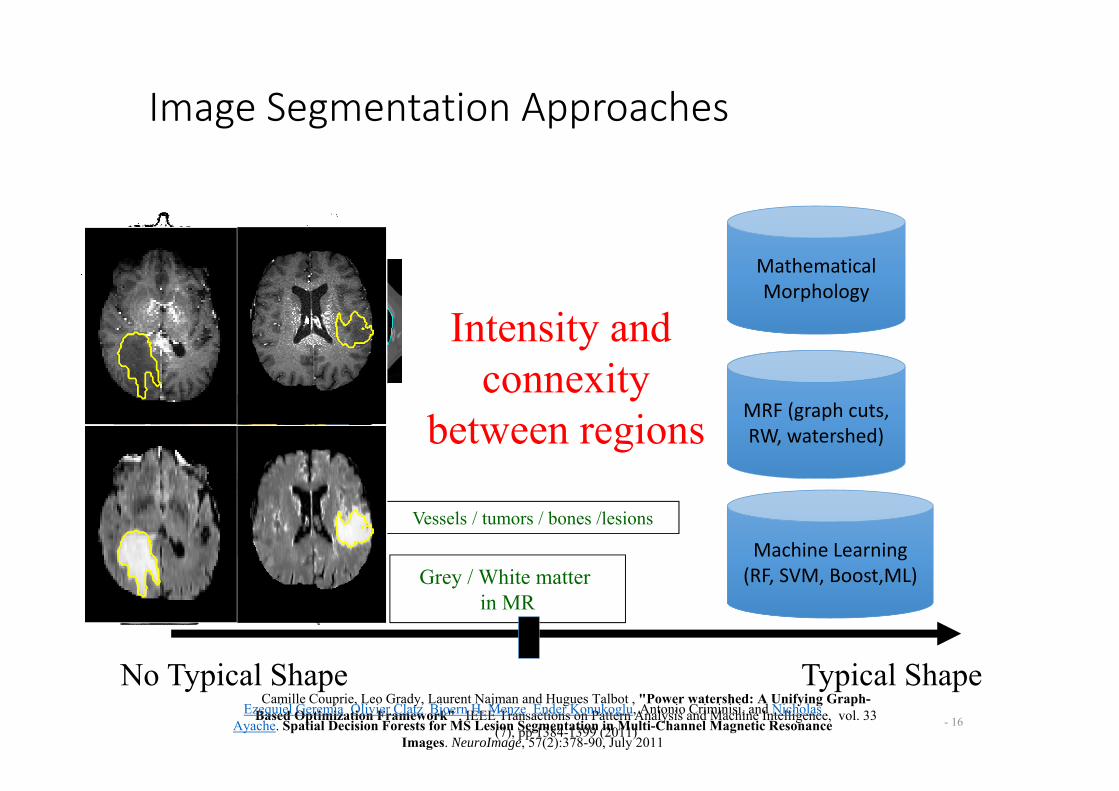
Image Segmentation Approaches
- 16
No Typical Shape Typical Shape
Grey / White matter in MR
Vessels / tumors / bones /lesions
MathematicalMorphology
MRF (graph cuts, RW, watershed)
Intensity and connexity
between regions
Machine Learning (RF, SVM, Boost,ML)
Camille Couprie, Leo Grady, Laurent Najman and Hugues Talbot , "Power watershed: A Unifying Graph-Based Optimization Framework" , IEEE Transactions on Pattern Analysis and Machine Intelligence, vol. 33
(7), pp 1384-1399 (2011)
Ezequiel Geremia, Olivier Clatz, Bjoern H. Menze, Ender Konukoglu, Antonio Criminisi, and Nicholas Ayache. Spatial Decision Forests for MS Lesion Segmentation in Multi-Channel Magnetic Resonance
Images. NeuroImage, 57(2):378-90, July 2011
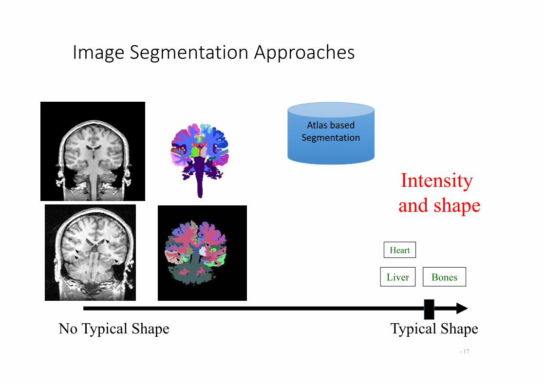
Image Segmentation Approaches
- 17
No Typical Shape Typical Shape
Liver
Heart
Bones
Atlas based Segmentation
Intensity and shape
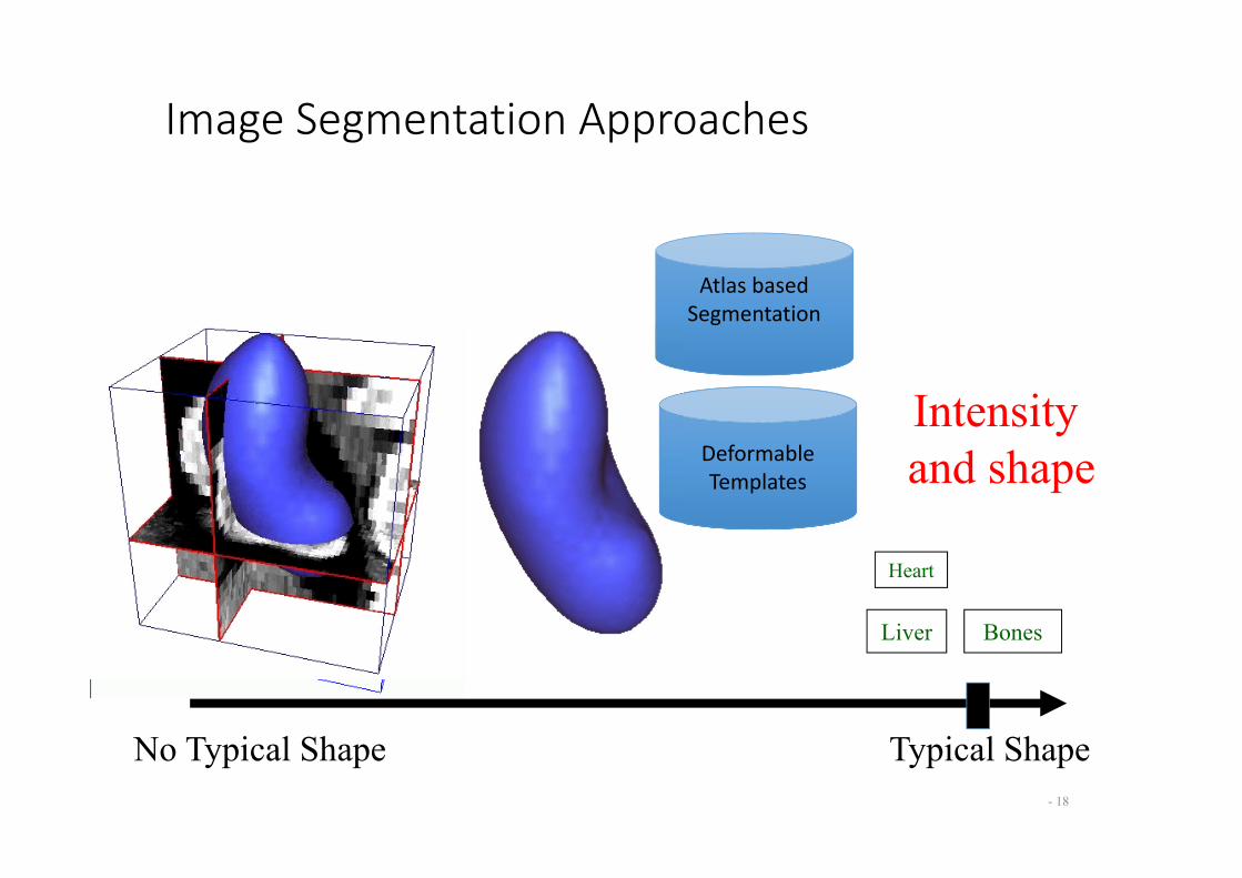
Image Segmentation Approaches
- 18
No Typical Shape Typical Shape
Liver
Heart
Atlas based Segmentation
Deformable Templates
Intensity and shape
Bones
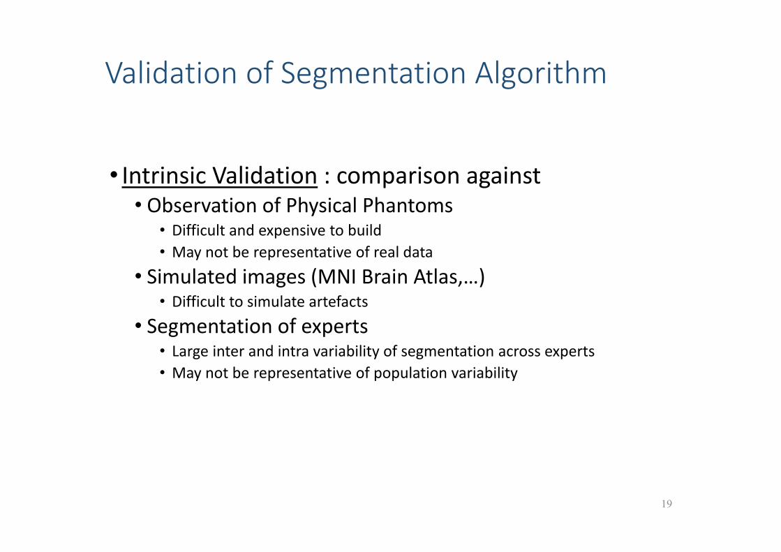
Validation of Segmentation Algorithm
• Intrinsic Validation : comparison against• Observation of Physical Phantoms
• Difficult and expensive to build• May not be representative of real data
• Simulated images (MNI Brain Atlas,…)• Difficult to simulate artefacts
• Segmentation of experts • Large inter and intra variability of segmentation across experts• May not be representative of population variability
19
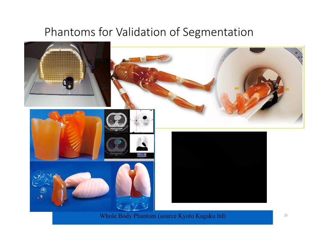
Phantoms for Validation of Segmentation
Whole Body Phantom (source Kyoto Kagaku ltd) 20
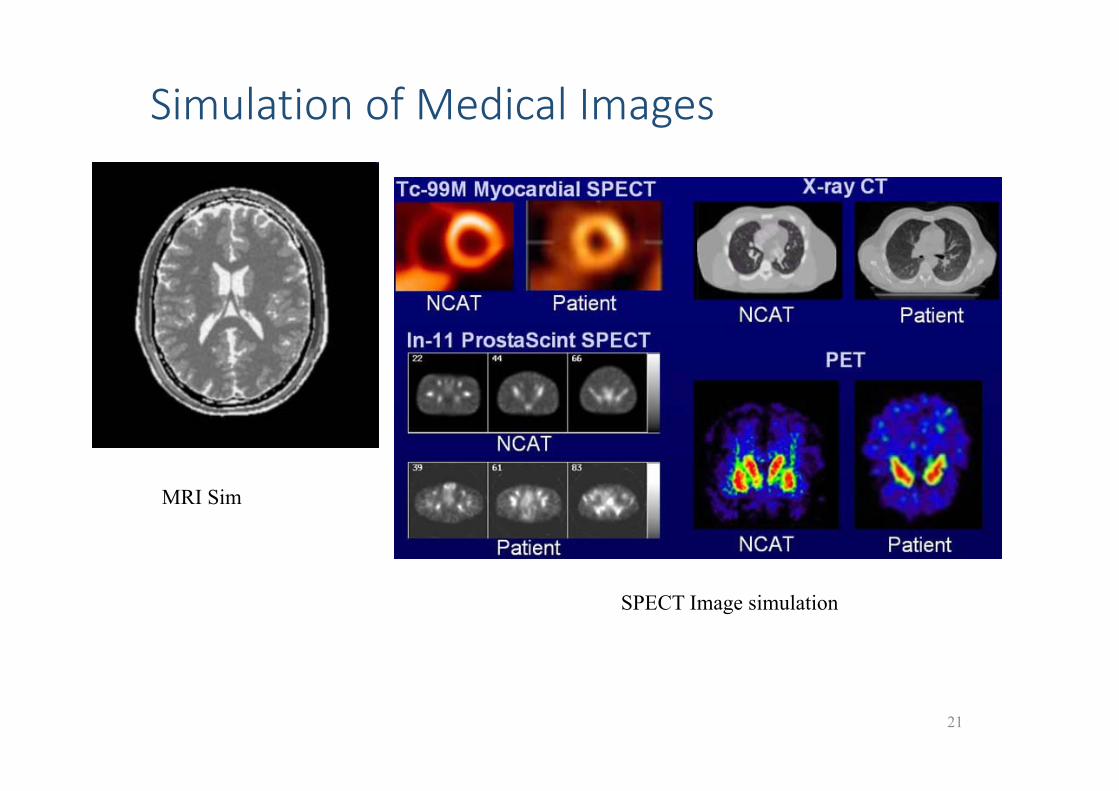
Simulation of Medical Images
MRI Sim
SPECT Image simulation
21
22
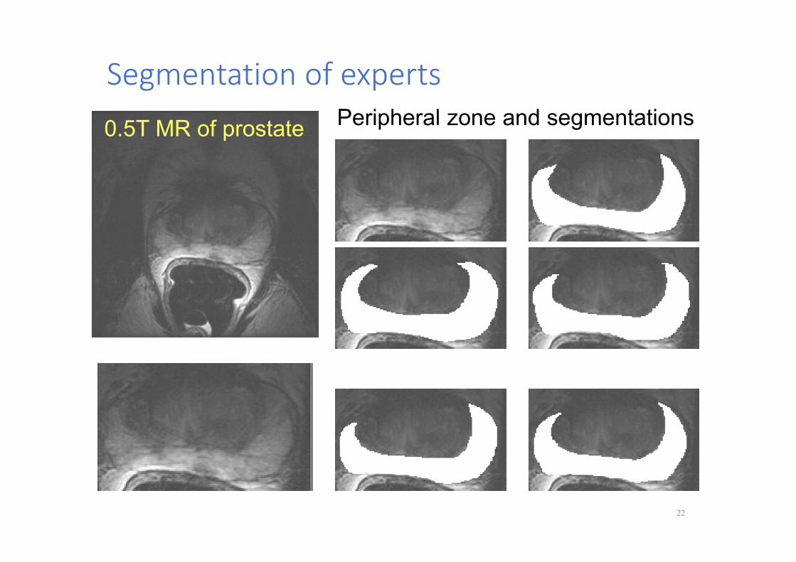
0.5T MR of prostate Peripheral zone and segmentations
Segmentation of experts
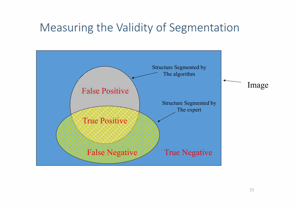
Measuring the Validity of Segmentation
23
Image
Structure Segmented byThe algorithm
Structure Segmented byThe expert
True Negative
True Positive
False Positive
False Negative
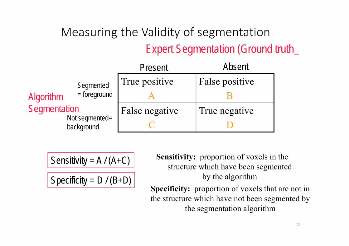
Measuring the Validity of segmentation
True positiveA
False positiveB
False negativeC
True negativeD
24
Expert Segmentation (Ground truth_ Present Absent
Segmented= foreground
Not segmented=background
Algorithm Segmentation
Sensitivity = A / (A+C)
Specificity = D / (B+D)
Sensitivity: proportion of voxels in the structure which have been segmented
by the algorithm Specificity: proportion of voxels that are not in the structure which have not been segmented by
the segmentation algorithm
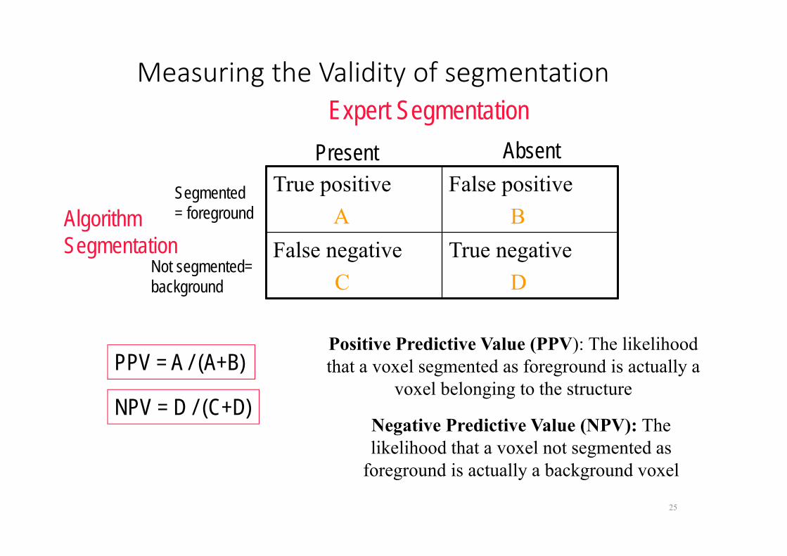
Measuring the Validity of segmentation
True positiveA
False positiveB
False negativeC
True negativeD
25
Expert Segmentation Present Absent
Segmented= foreground
Not segmented=background
Algorithm Segmentation
PPV = A / (A+B)
NPV = D / (C+D)
Positive Predictive Value (PPV): The likelihood that a voxel segmented as foreground is actually a
voxel belonging to the structure
Negative Predictive Value (NPV): The likelihood that a voxel not segmented as
foreground is actually a background voxel
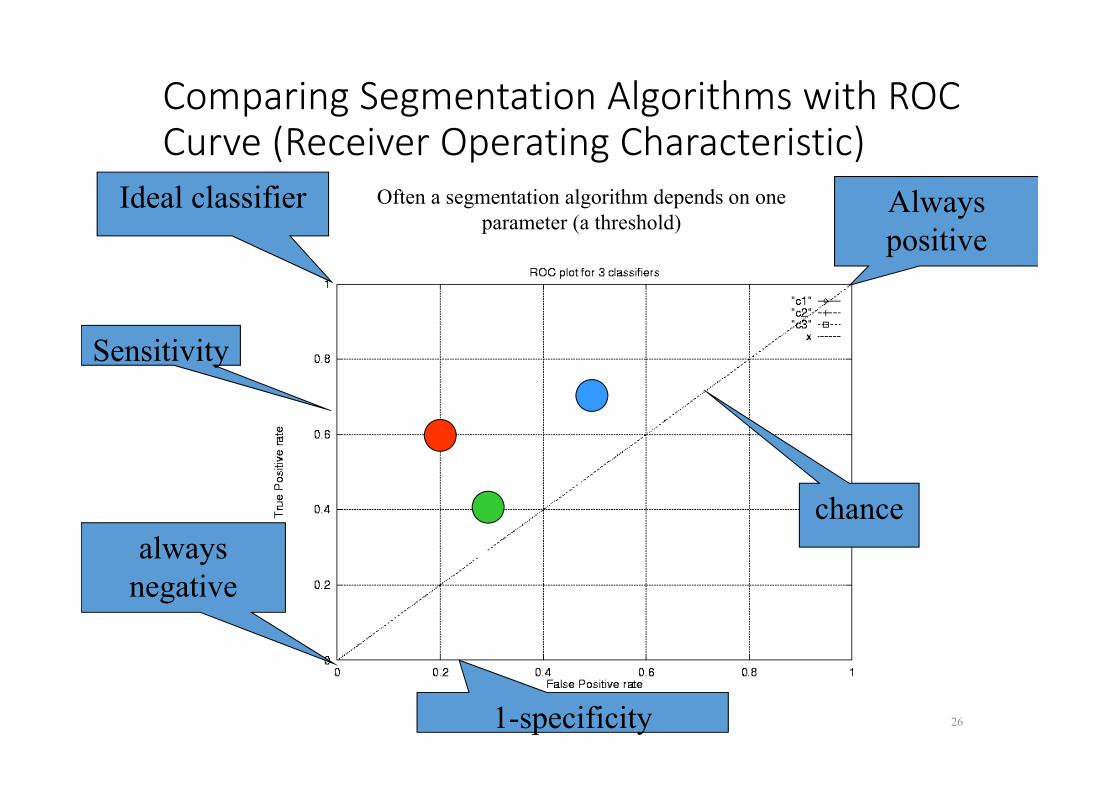
Comparing Segmentation Algorithms with ROC Curve (Receiver Operating Characteristic)
26
Ideal classifier
chance
1-specificity
Sensitivity
always negative
Always positive
Often a segmentation algorithm depends on one parameter (a threshold)
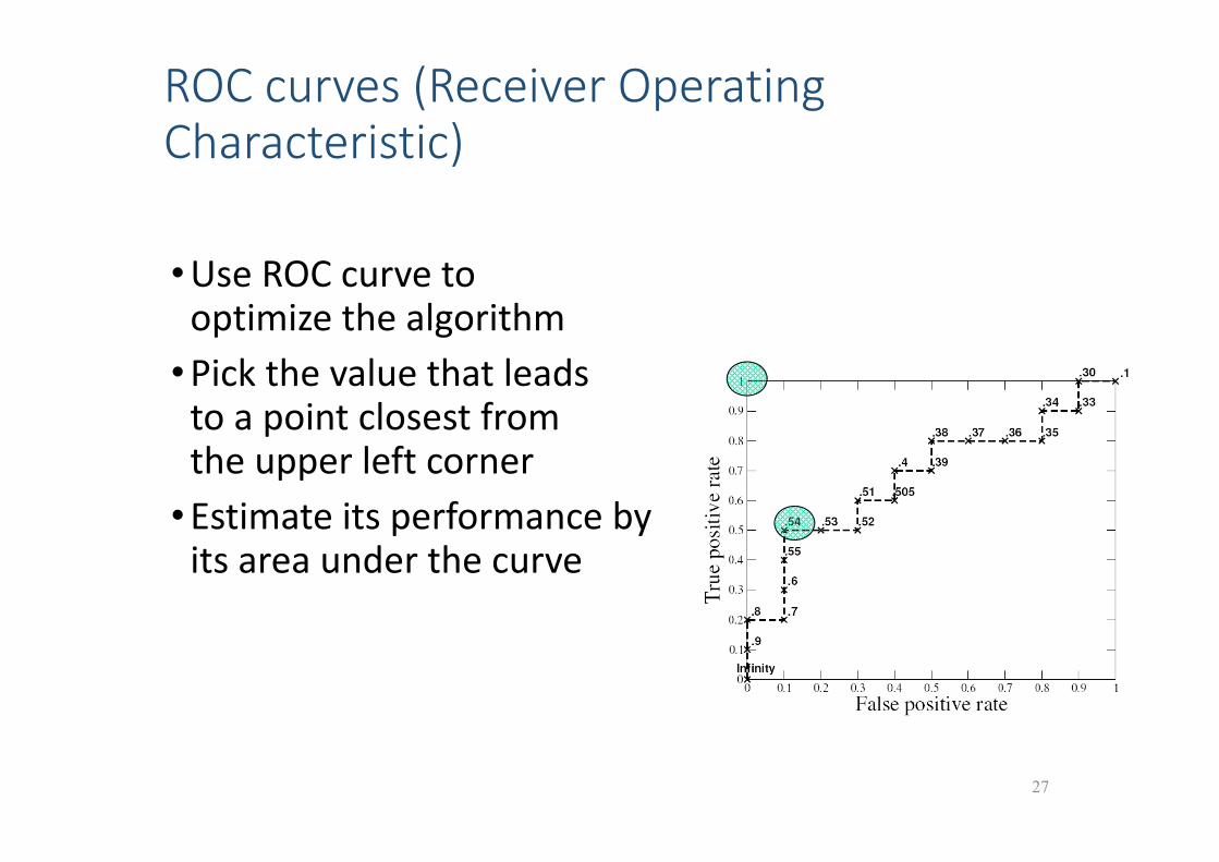
ROC curves (Receiver Operating Characteristic)
•Use ROC curve tooptimize the algorithm
•Pick the value that leadsto a point closest fromthe upper left corner
•Estimate its performance byits area under the curve
27
Other measures of segmentation Performance
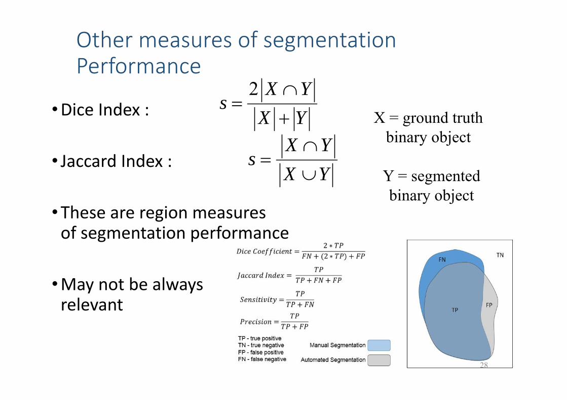
•Dice Index :
• Jaccard Index :
•These are region measures of segmentation performance
•May not be alwaysrelevant
28
YXYX
s
2
X = ground truthbinary object
Y = segmented binary object
YXYX
s
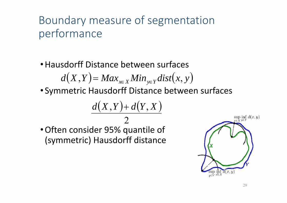
Boundary measure of segmentation performance
•Hausdorff Distance between surfaces
•Symmetric Hausdorff Distance between surfaces
•Often consider 95% quantile of (symmetric) Hausdorff distance
29
yxdistMinMaxYXd YyXx ,,
2
,, XYdYXd
Validation of Segmentation Algorithm (2)
•Extrinsic Validation : comparison against other segmentation algorithms
• Only possible when no ground truth exists (Inter‐patient registration of images) or when it is not available
• Estimate consistency, repeatability and size of convergence basin
30
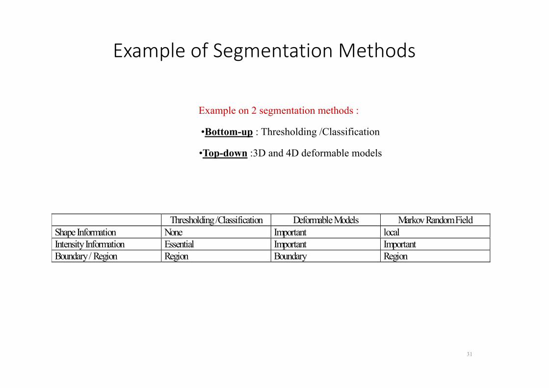
Example of Segmentation Methods
Example on 2 segmentation methods :
•Bottom-up : Thresholding /Classification
•Top-down :3D and 4D deformable models
Thresholding /Classification Deformable Models Markov Random FieldShape Information None Important localIntensity Information Essential Important ImportantBoundary / Region Region Boundary Region
31
Segmentation
2 Filtering and Thresholding
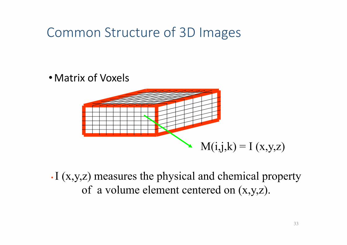
Common Structure of 3D Images
•Matrix of Voxels
33
M(i,j,k) = I (x,y,z)
• I (x,y,z) measures the physical and chemical propertyof a volume element centered on (x,y,z).
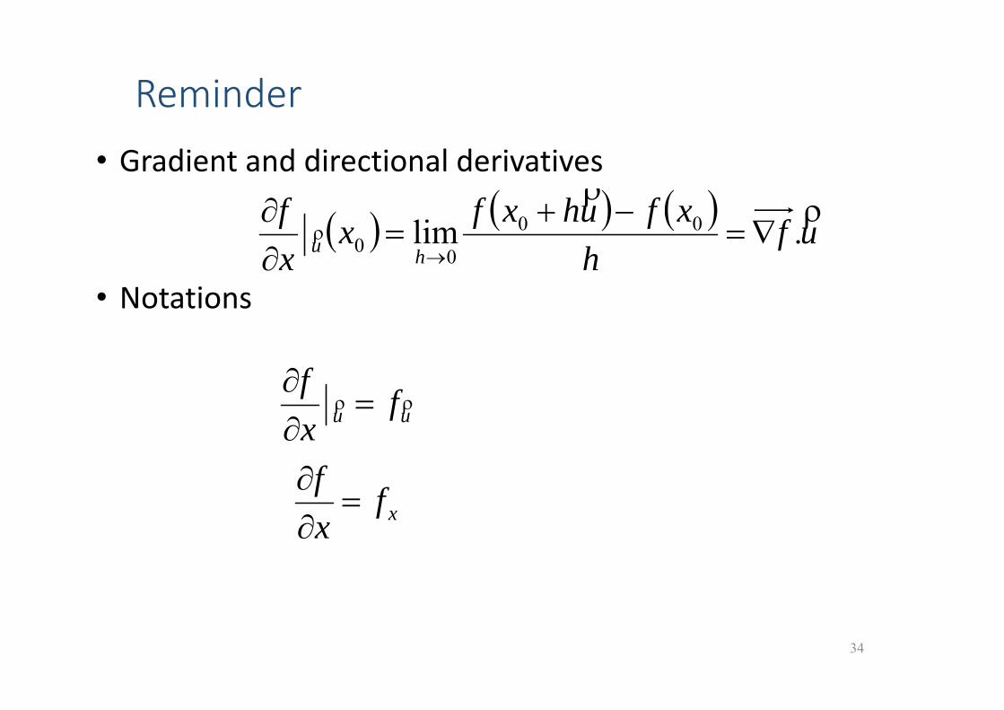
Reminder• Gradient and directional derivatives
• Notations
34
ufh
xfuhxfxxf
hu
.lim 00
00
uu fxf
xfxf
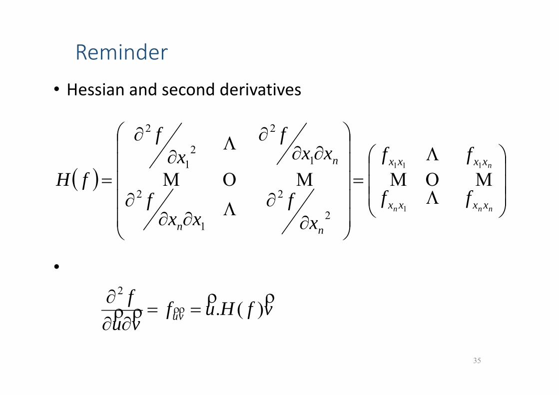
Reminder• Hessian and second derivatives
•
35
nnn
n
xxxx
xxxx
nn
n
ff
ff
xf
xxf
xxf
xf
fH
1
111
2
2
1
2
1
2
21
2
vfHufvuf
vu
)(.2
Image Segmentation
• 2 dual approaches : • Contour Detection:
Find voxels with discontinuities of intensity
• Region Approach :Find Regions with homogeneous intensity or texture
•Other feature detection :• Corner detection• Blob detection• SIFT
36
Need to extract featurebased on image filtering
Segmentation
2 Filtering and Thresholding
2.1 Filtering
Image Filtering
•Overview :• Linear vs Non‐Linear• Separable vs Non‐Separable• Recursive Filters• Smoothing Filters :
• Discrete vs Continous• Isotropic vs Anisotropic• Recursive• Non‐Local
• Gradient Filters :• Discrete vs Continuous
38

Image Filtering
• Image Filtering consists in extracting local information : basis for feature extraction
• Different types of filters:• Linear : = Convolution with a function (filter) • Non‐linear• Separable : a nD filter may be written as the composition of several 1D filters
• Non‐separable
39
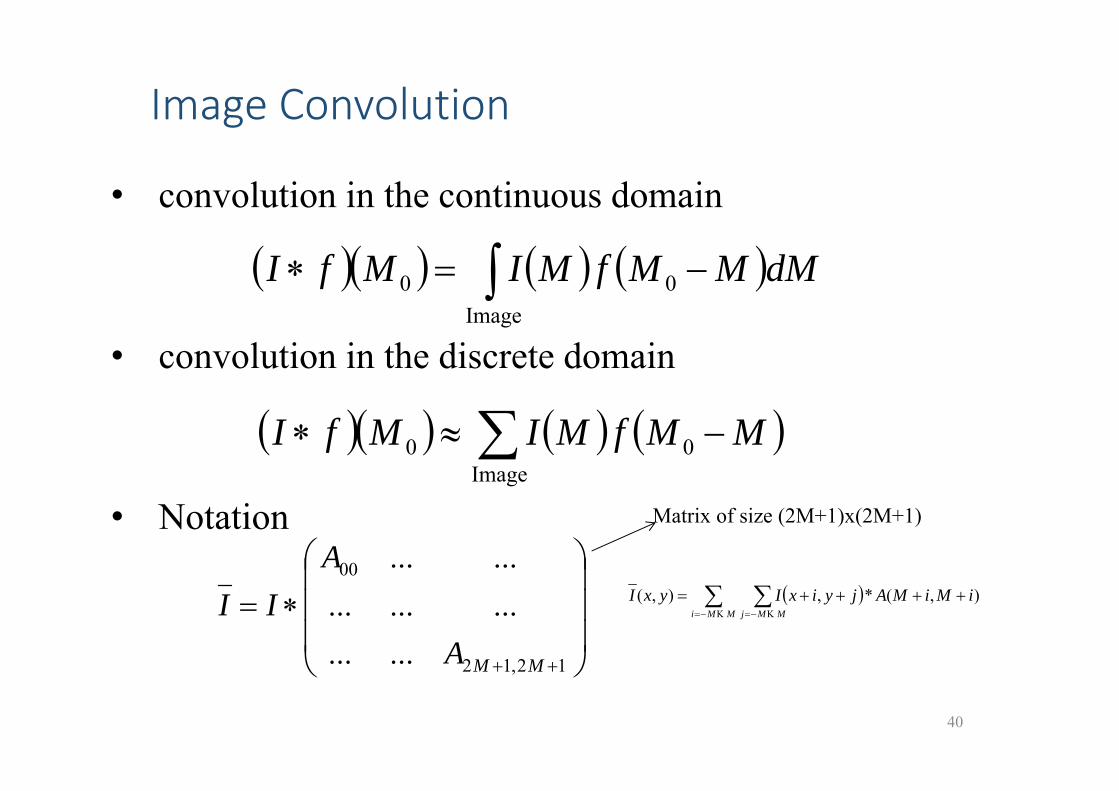
Image Convolution
40
• convolution in the continuous domain
• convolution in the discrete domain
• Notation
Image
00 dMMMfMIMfI
Image
00 MMfMIMfI
),(*,),( iMiMAjyixIyxIMMi MMj
12,12
00
.....................
MMA
AII
Matrix of size (2M+1)x(2M+1)
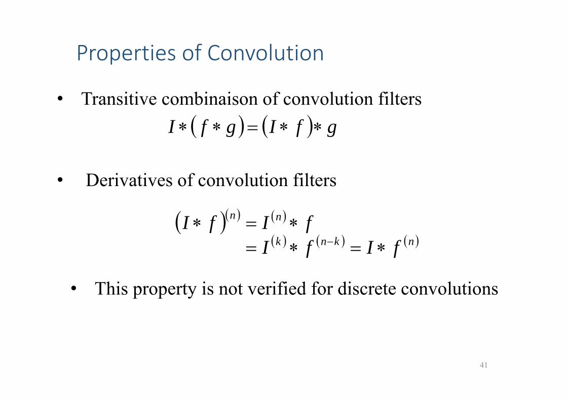
Properties of Convolution
41
• Transitive combinaison of convolution filters
• Derivatives of convolution filters
• This property is not verified for discrete convolutions
gfIgfI
nknk
nn
fIfIfIfI
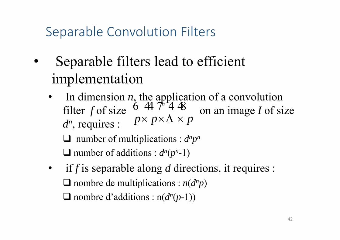
Separable Convolution Filters
42
• Separable filters lead to efficient implementation
• In dimension n, the application of a convolution filter f of size on an image I of size dn, requires : number of multiplications : dnpn
number of additions : dn(pn-1)
• if f is separable along d directions, it requires : nombre de multiplications : n(dnp) nombre d’additions : n(dn(p-1))
n
ppp
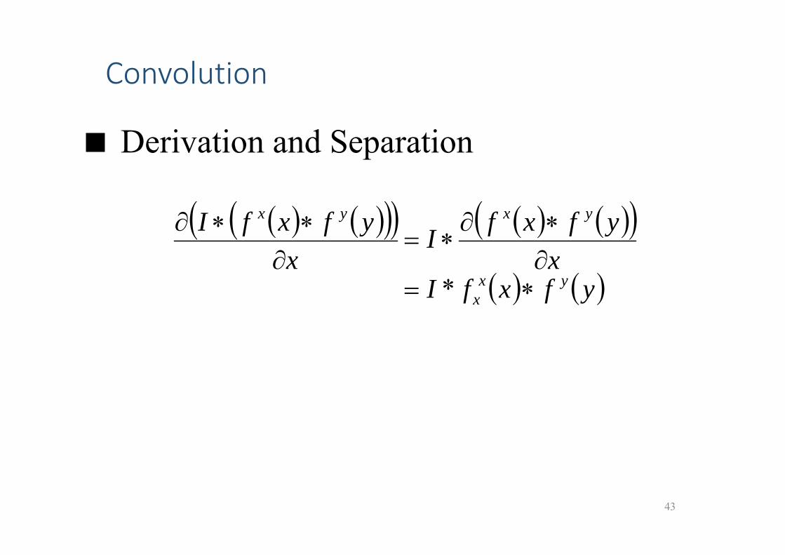
Convolution
43
Derivation and Separation
yfxfIx
yfxfIx
yfxfI
yxx
yxyx
*
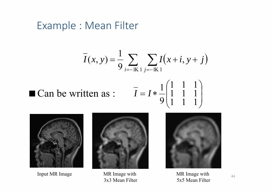
Example : Mean Filter
44
Can be written as :
11 11
,91),(
i jjyixIyxI
111111111
91II
Input MR Image MR Image with 3x3 Mean Filter
MR Image with 5x5 Mean Filter
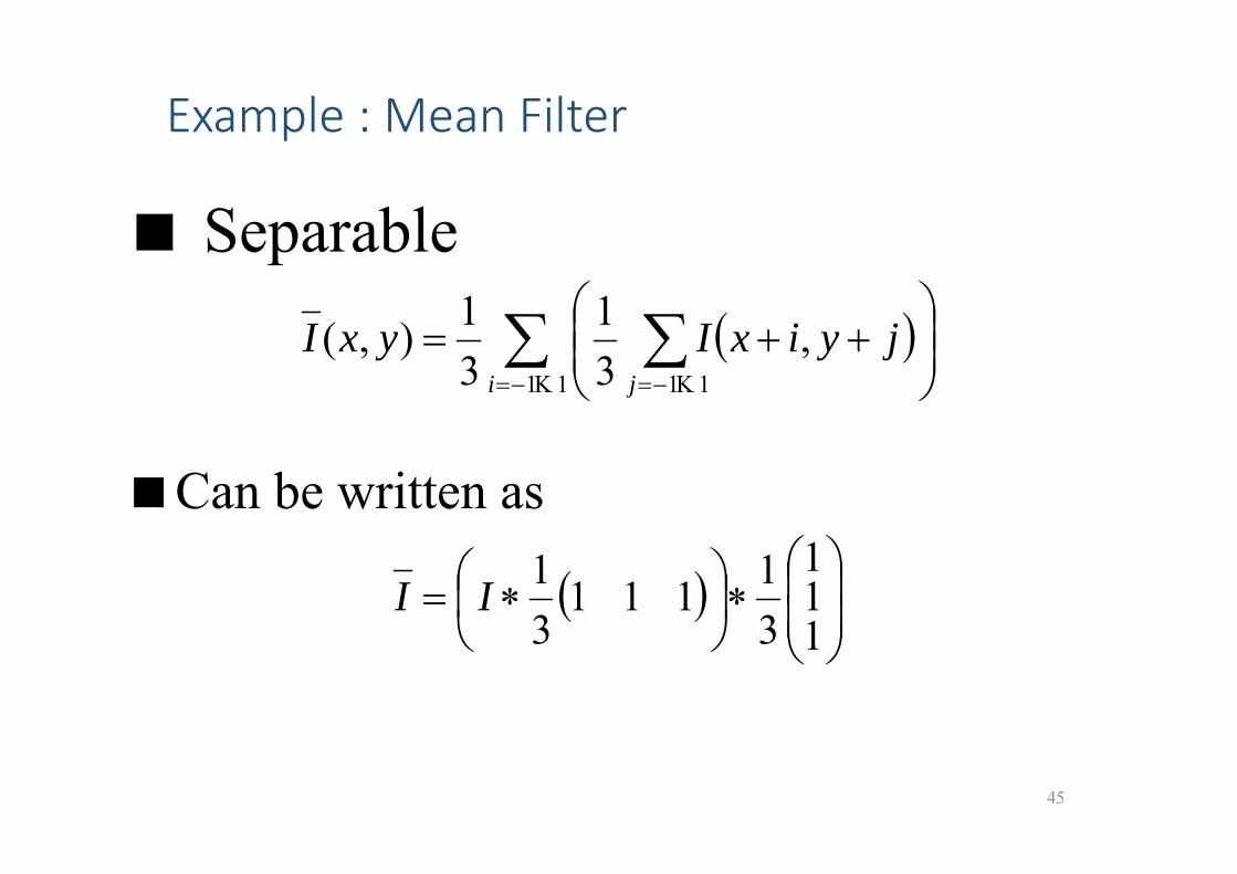
Example : Mean Filter
45
Separable
Can be written as
11 11
,31
31),(
i j
jyixIyxI
111
31111
31II
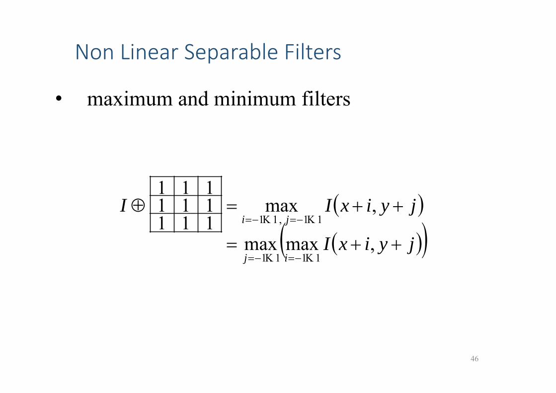
Non Linear Separable Filters
46
• maximum and minimum filters
jyixI
jyixII
ij
ji
,maxmax
,max111111111
1111
11 , 11
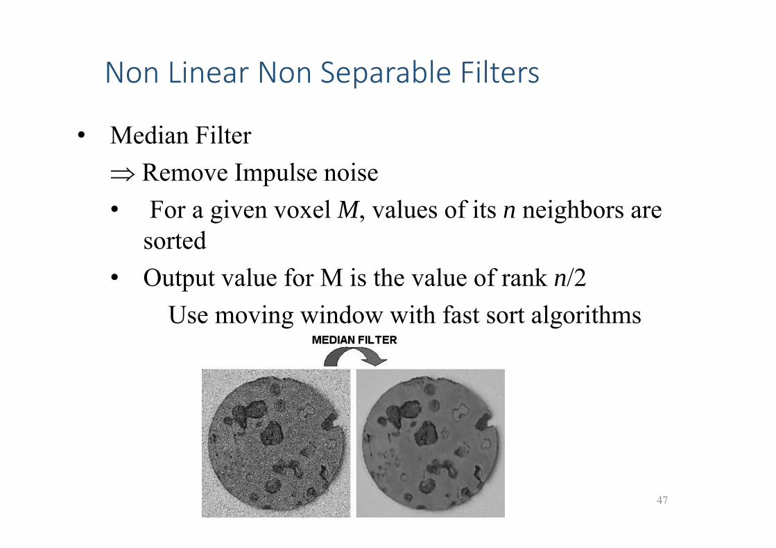
Non Linear Non Separable Filters
47
• Median Filter Remove Impulse noise• For a given voxel M, values of its n neighbors are
sorted• Output value for M is the value of rank n/2
Use moving window with fast sort algorithms(quicksort, …)
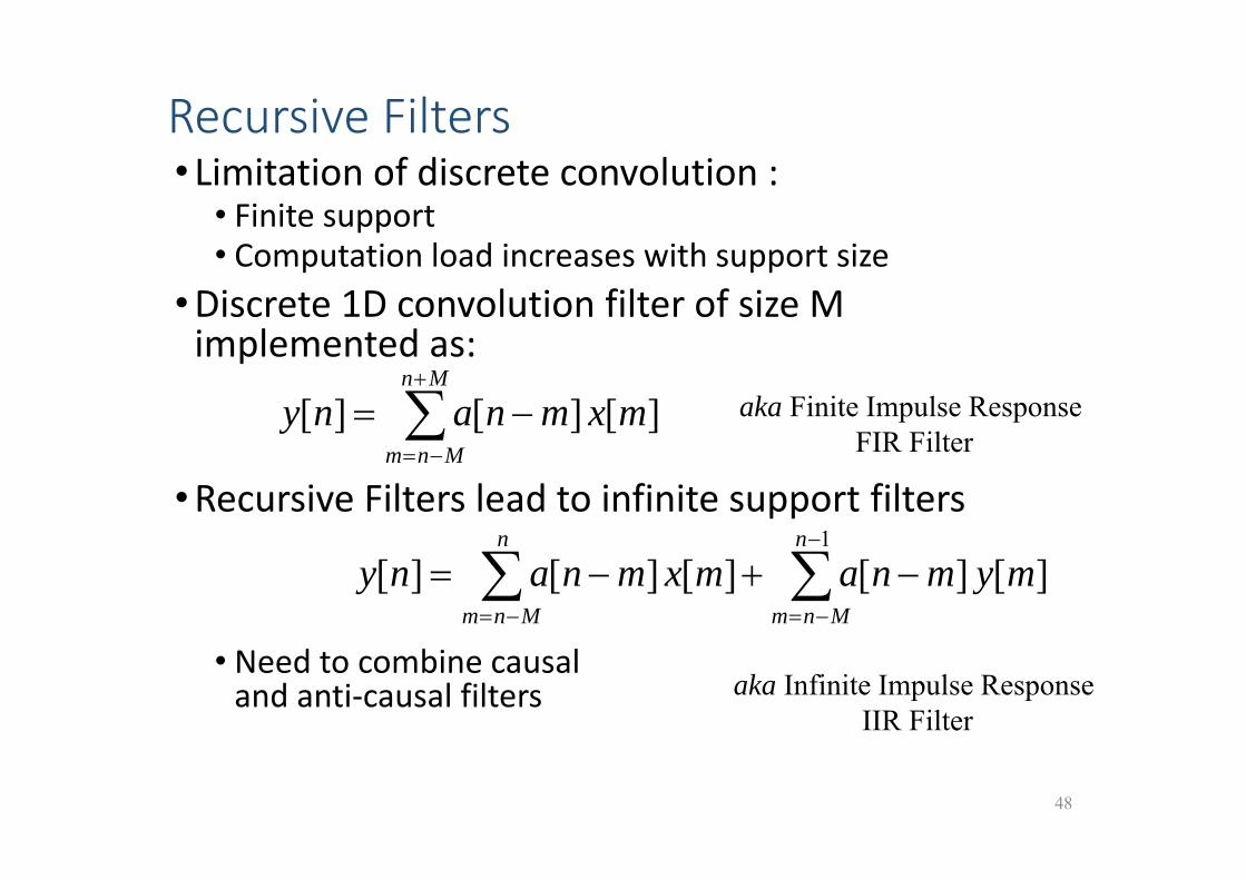
Recursive Filters• Limitation of discrete convolution :
• Finite support• Computation load increases with support size
•Discrete 1D convolution filter of size M implemented as:
•Recursive Filters lead to infinite support filters
• Need to combine causal and anti‐causal filters
48
Mn
Mnmmxmnany ][][][ aka Finite Impulse Response
FIR Filter
1
][][][][][n
Mnm
n
Mnmmymnamxmnany
aka Infinite Impulse Response IIR Filter
Image Filtering
•Overview :• Linear vs Non‐Linear• Separable vs Non‐Separable• Recursive Filters• Smoothing Filters :
• Discrete vs Continous• Isotropic vs Anisotropic• Recursive• Non‐Local
• Gradient Filters :• Discrete vs Continuous
49
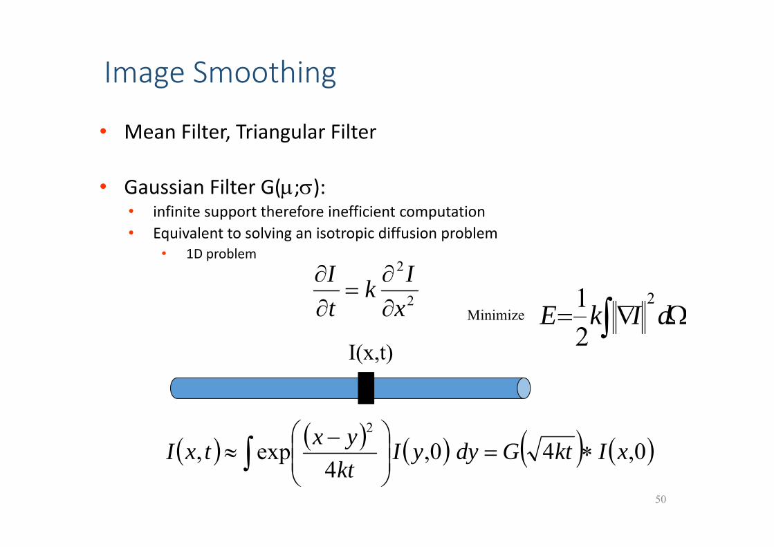
Image Smoothing
• Mean Filter, Triangular Filter
• Gaussian Filter G(;): • infinite support therefore inefficient computation• Equivalent to solving an isotropic diffusion problem
• 1D problem
50
2
2
xIk
tI
0,40,4
exp,2
xIktGdyyIktyxtxI
I(x,t) dIkE
2
21
Minimize
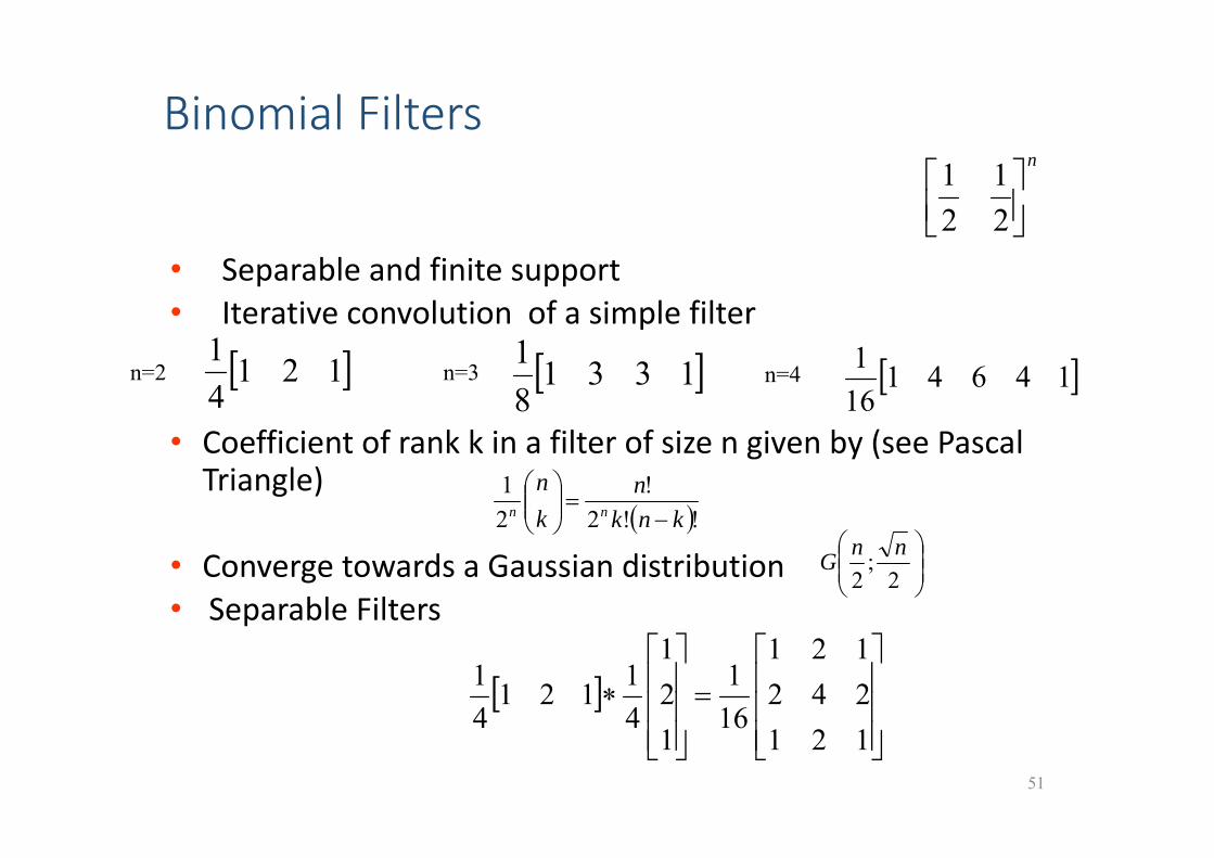
Binomial Filters
• Separable and finite support• Iterative convolution of a simple filter
• Coefficient of rank k in a filter of size n given by (see Pascal Triangle)
• Converge towards a Gaussian distribution• Separable Filters
51
2;
2nnG
121242121
161
121
41121
41
!!2!
21
knkn
kn
nn
n
21
21
12141 1331
81 14641
161n=2 n=3 n=4
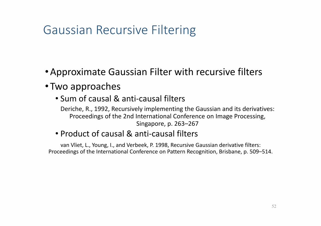
Gaussian Recursive Filtering
•Approximate Gaussian Filter with recursive filters•Two approaches
• Sum of causal & anti‐causal filtersDeriche, R., 1992, Recursively implementing the Gaussian and its derivatives:
Proceedings of the 2nd International Conference on Image Processing, Singapore, p. 263–267
• Product of causal & anti‐causal filtersvan Vliet, L., Young, I., and Verbeek, P. 1998, Recursive Gaussian derivative filters:
Proceedings of the International Conference on Pattern Recognition, Brisbane, p. 509–514.
52
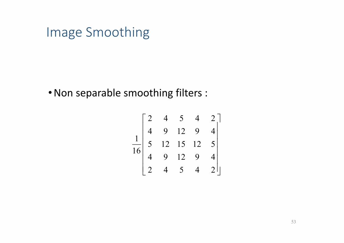
Image Smoothing
•Non separable smoothing filters :
53
245424912945121512549129424542
161
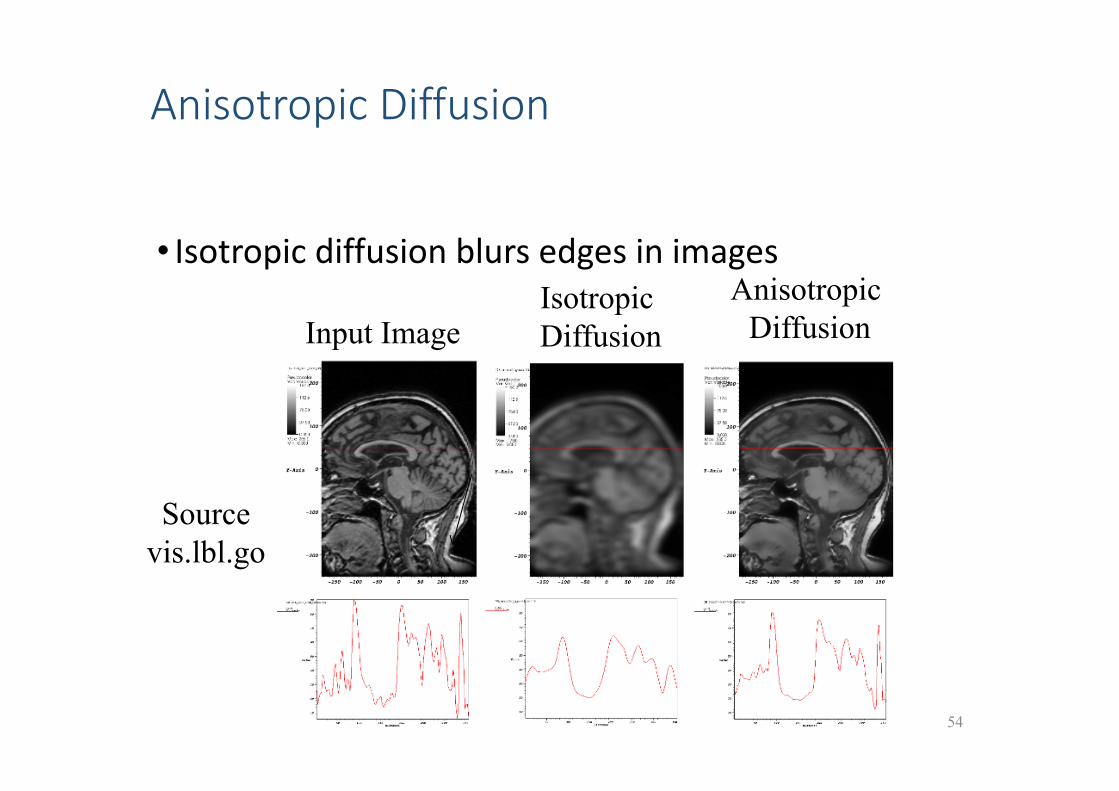
Anisotropic Diffusion
• Isotropic diffusion blurs edges in images
54
Input ImageIsotropic Diffusion
Anisotropic Diffusion
Sourcevis.lbl.go
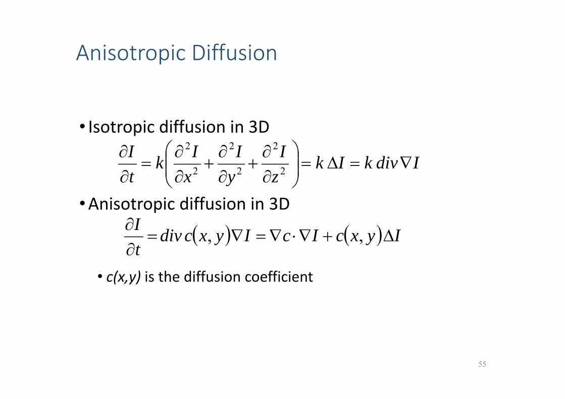
Anisotropic Diffusion
• Isotropic diffusion in 3D
•Anisotropic diffusion in 3D
• c(x,y) is the diffusion coefficient
55
IdivkIkzI
yI
xIk
tI
2
2
2
2
2
2
IyxcIcIyxcdivtI
,,
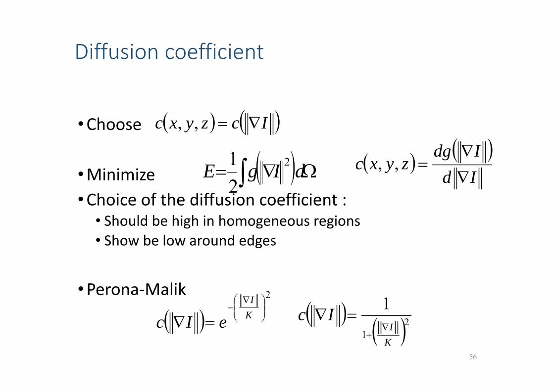
Diffusion coefficient
•Choose
•Minimize•Choice of the diffusion coefficient :
• Should be high in homogeneous regions• Show be low around edges
•Perona‐Malik
56
2
KI
eIc 21
1
KI
Ic
Iczyxc ,,
dIgE 2
21
IdIdg
zyxc
,,
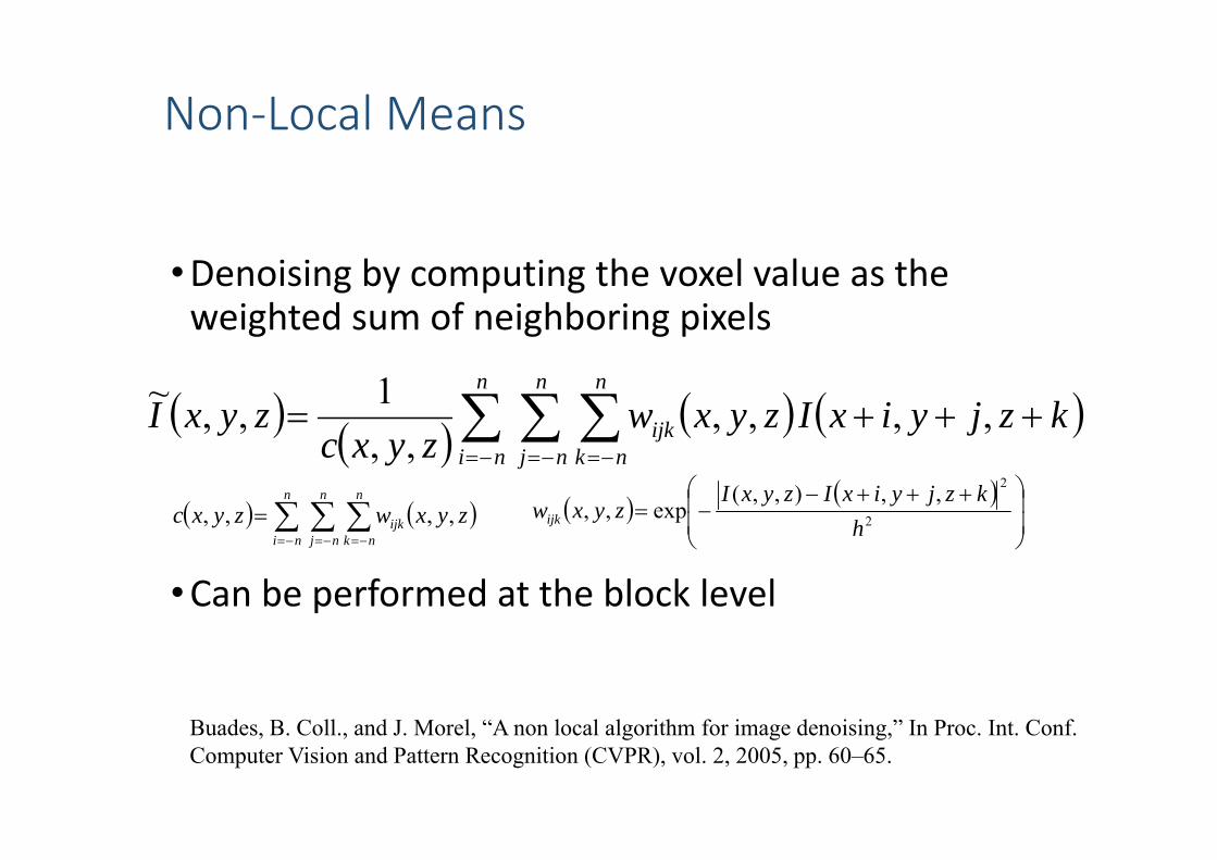
Non‐Local Means
•Denoising by computing the voxel value as the weighted sum of neighboring pixels
•Can be performed at the block level
57
n
ni
n
nj
n
nkijk kzjyixIzyxw
zyxczyxI ,,,,
,,1,,~
n
ni
n
nj
n
nkijk zyxwzyxc ,,,,
2
2,,),,(exp,,
hkzjyixIzyxI
zyxwijk
Buades, B. Coll., and J. Morel, “A non local algorithm for image denoising,” In Proc. Int. Conf. Computer Vision and Pattern Recognition (CVPR), vol. 2, 2005, pp. 60–65.
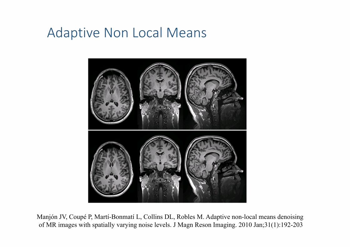
Adaptive Non Local Means
58Manjón JV, Coupé P, Martí-Bonmatí L, Collins DL, Robles M. Adaptive non-local means denoisingof MR images with spatially varying noise levels. J Magn Reson Imaging. 2010 Jan;31(1):192-203
Image Filtering
•Overview :• Linear vs Non‐Linear• Separable vs Non‐Separable• Recursive Filters• Smoothing Filters :
• Discrete vs Continous• Isotropic vs Anisotropic• Recursive• Non‐Local
• Gradient Filters :• Discrete vs Continuous
59
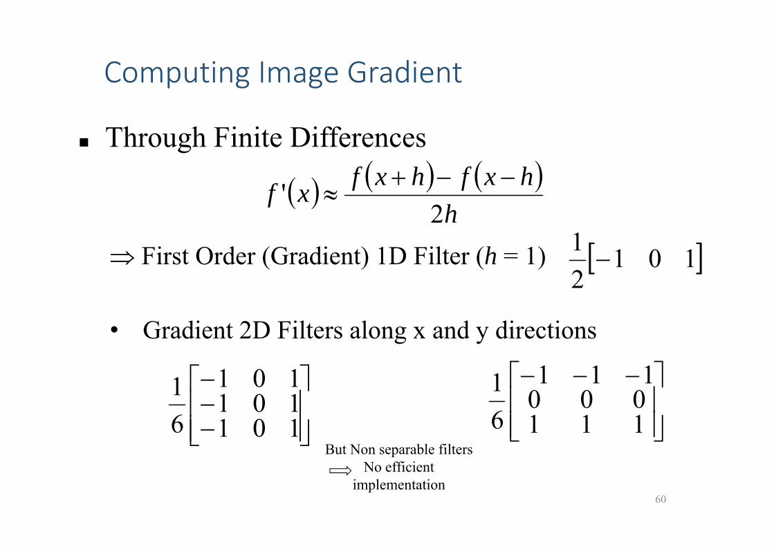
Computing Image Gradient
60
Through Finite Differences
First Order (Gradient) 1D Filter (h = 1)
• Gradient 2D Filters along x and y directions
h
hxfhxfxf2
'
10121
101101101
61
111000111
61
But Non separable filtersNo efficient
implementation
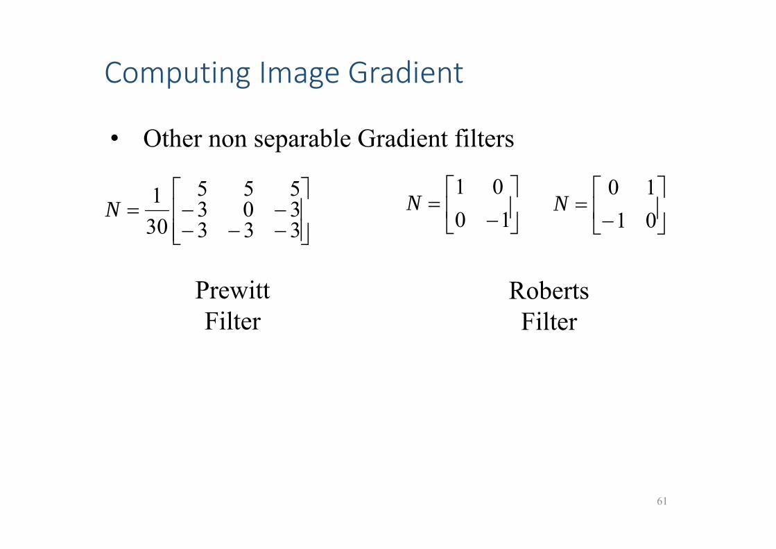
Computing Image Gradient
61
• Other non separable Gradient filters
333303555
301N
10
01N
RobertsFilter
PrewittFilter
0110
N

Sobel Filters
62
• Sobel Filters• Separable Filters• Reduce noise by convolving with low-pass filter
(remove high frequencies) : binomial filters• First Order along x
• First Order along y
101202101
81
121
41101
21
121000121
81
101
21121
41
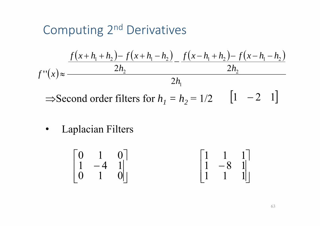
Computing 2nd Derivatives
63
Second order filters for h1 = h2 = 1/2
• Laplacian Filters
121
010141010
111181111
1
2
2121
2
2121
222''
hh
hhxfhhxfh
hhxfhhxf
xf
Segmentation
2 Filtering and Thresholding
2.2 Contour Detection
Overview
•Definitions of Image Contours• Maxima of gradient norm in the direction of Gradient• Zero crossing of Laplacian
•Optimal Filters • Canny & Deriche Filters
65

Contour Detection
• Qualitatively :Find points where I(x,y) varies very quickly with (x,y).
66
xI
I
2
2
xI
Contour Detection
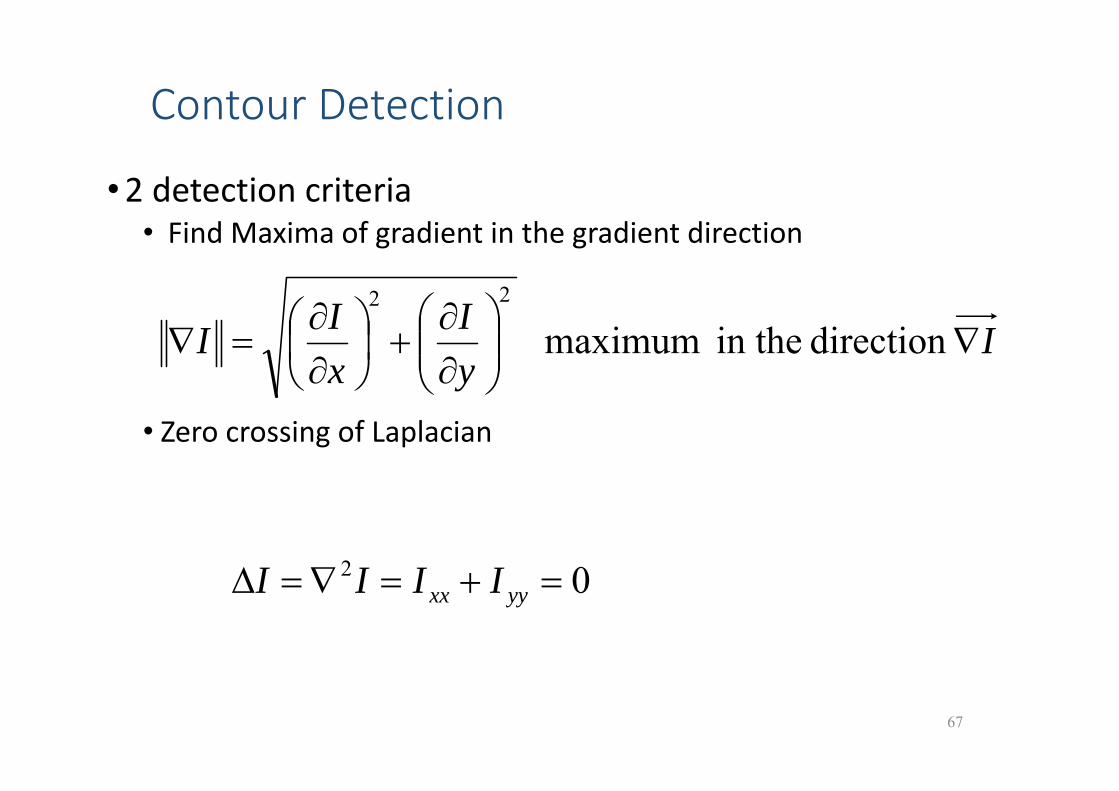
•2 detection criteria • Find Maxima of gradient in the gradient direction
• Zero crossing of Laplacian
67
IyI
xII
direction in the maximum 22
02 yyxx IIII
Gradient Maxima
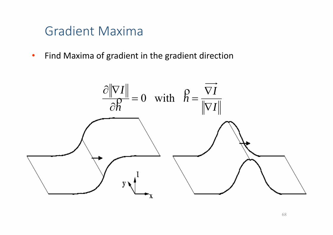
• Find Maxima of gradient in the gradient direction
68
IIn
nI
with 0
Gradient Maxima
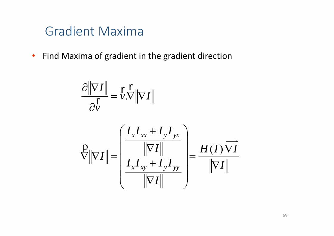
• Find Maxima of gradient in the gradient direction
69
IIIH
IIIII
IIIII
Iyyyxyx
yxyxxx
)(
Ivv
I
rrr .
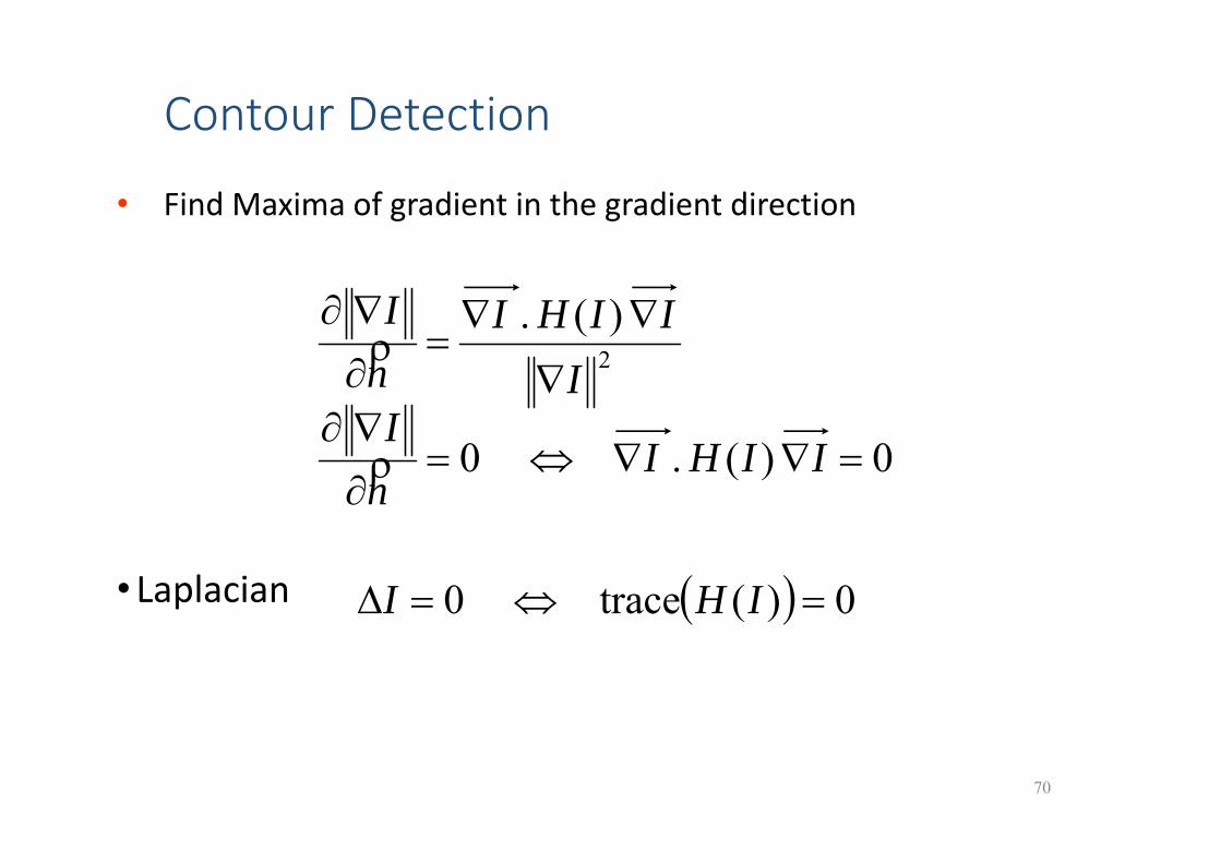
Contour Detection
• Find Maxima of gradient in the gradient direction
• Laplacian
70
2 )( .
IIIHI
nI
0 )( . 0
IIHInI
0)( trace 0 IHI
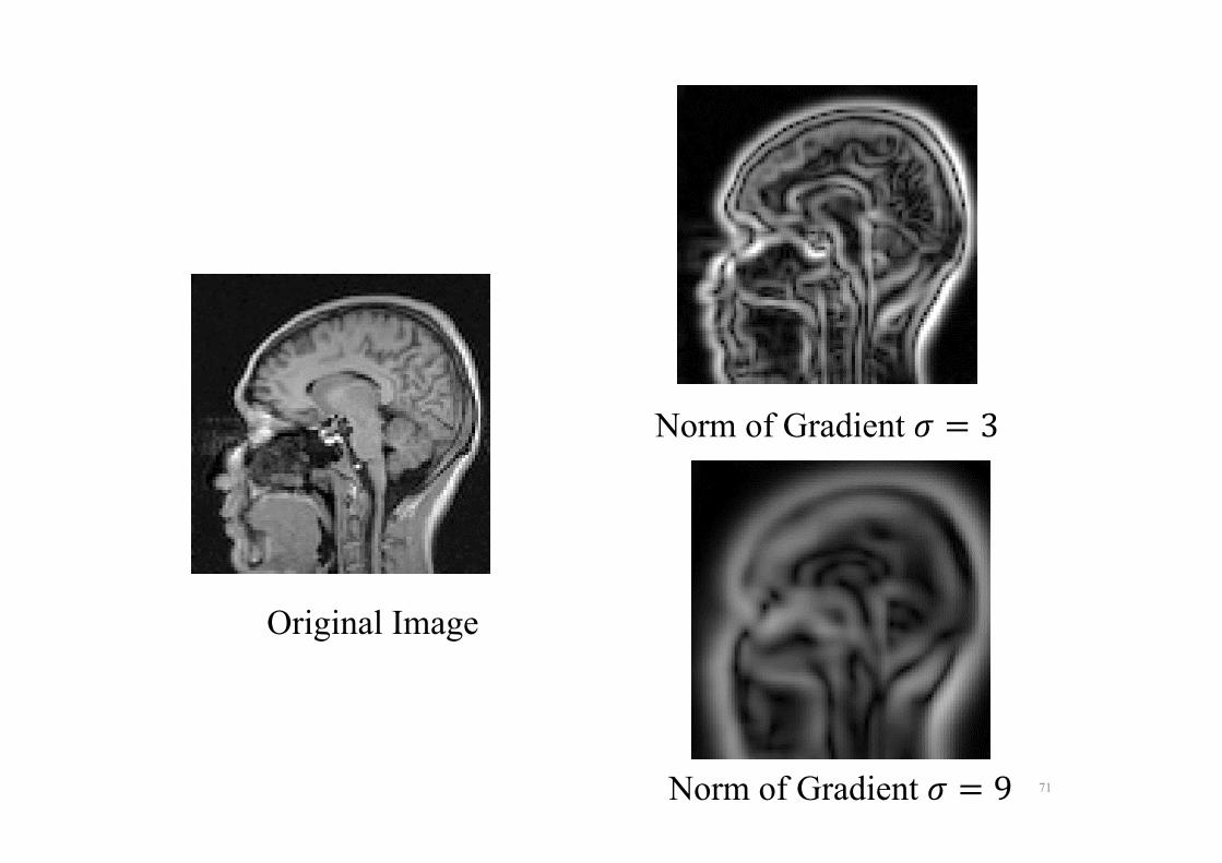
71
Original Image
Norm of Gradient 3
Norm of Gradient 9
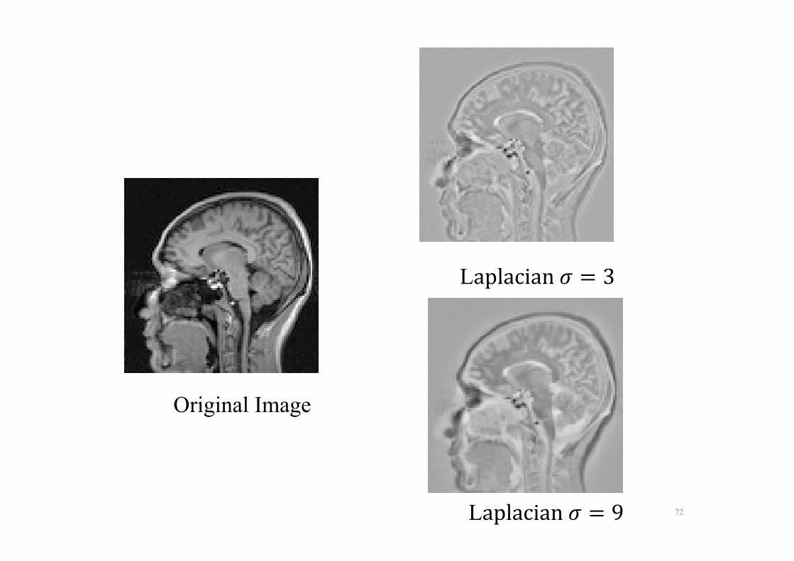
72
Original Image
Laplacian 3
Laplacian 9
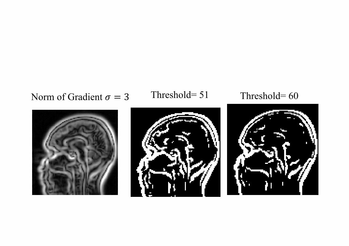
Threshold= 51
Gradient
Norm
Threshold= 60Norm of Gradient 3
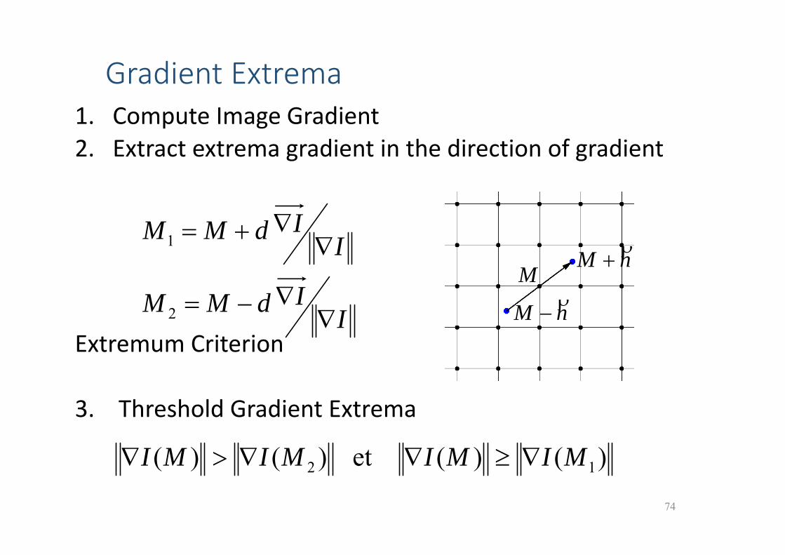
Gradient Extrema1. Compute Image Gradient2. Extract extrema gradient in the direction of gradient
Extremum Criterion
3. Threshold Gradient Extrema
74
IIdMM
1
IIdMM
2
)()(et )()( 12 MIMIMIMI
nM
M
nM
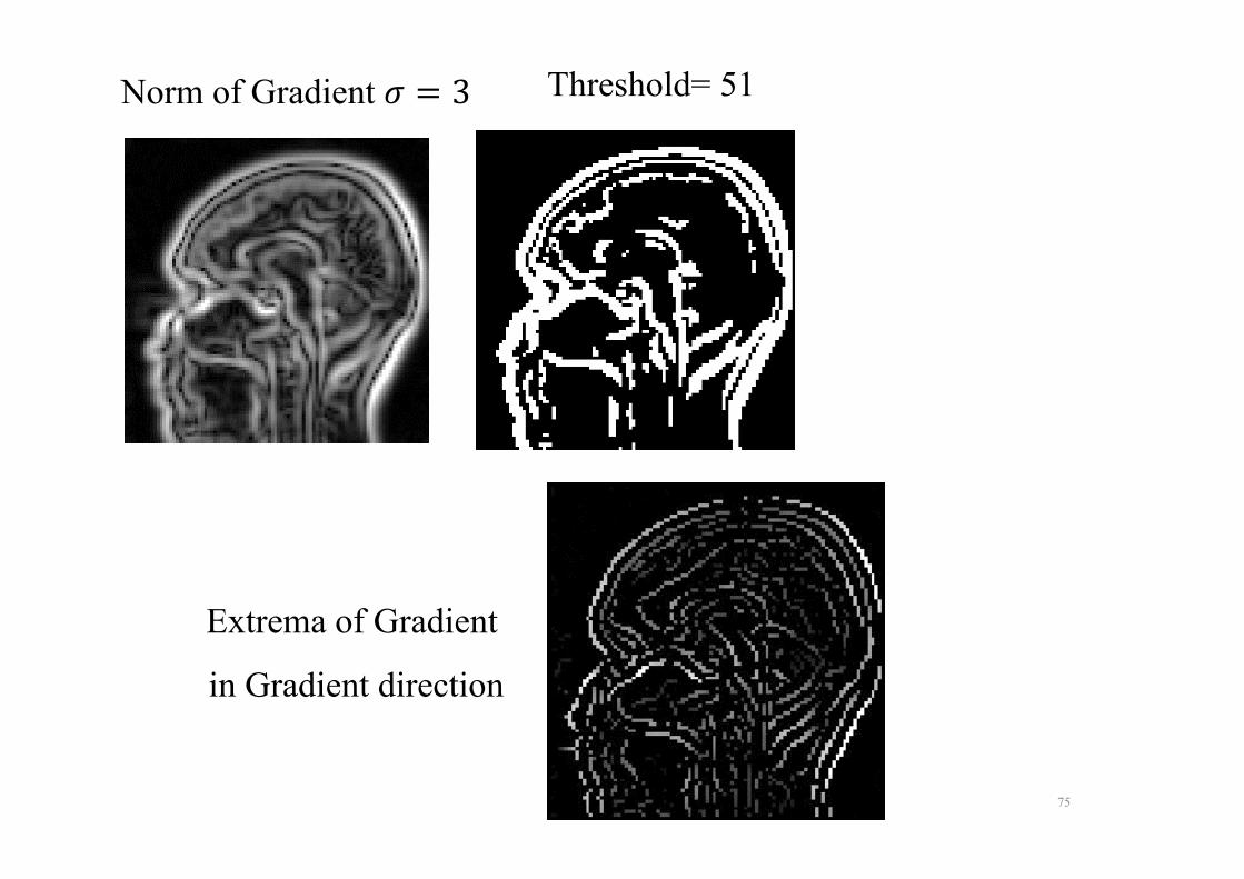
75
= 2
Extrema of Gradient
in Gradient direction
Threshold= 51
Gradient
Norm
Norm of Gradient 3
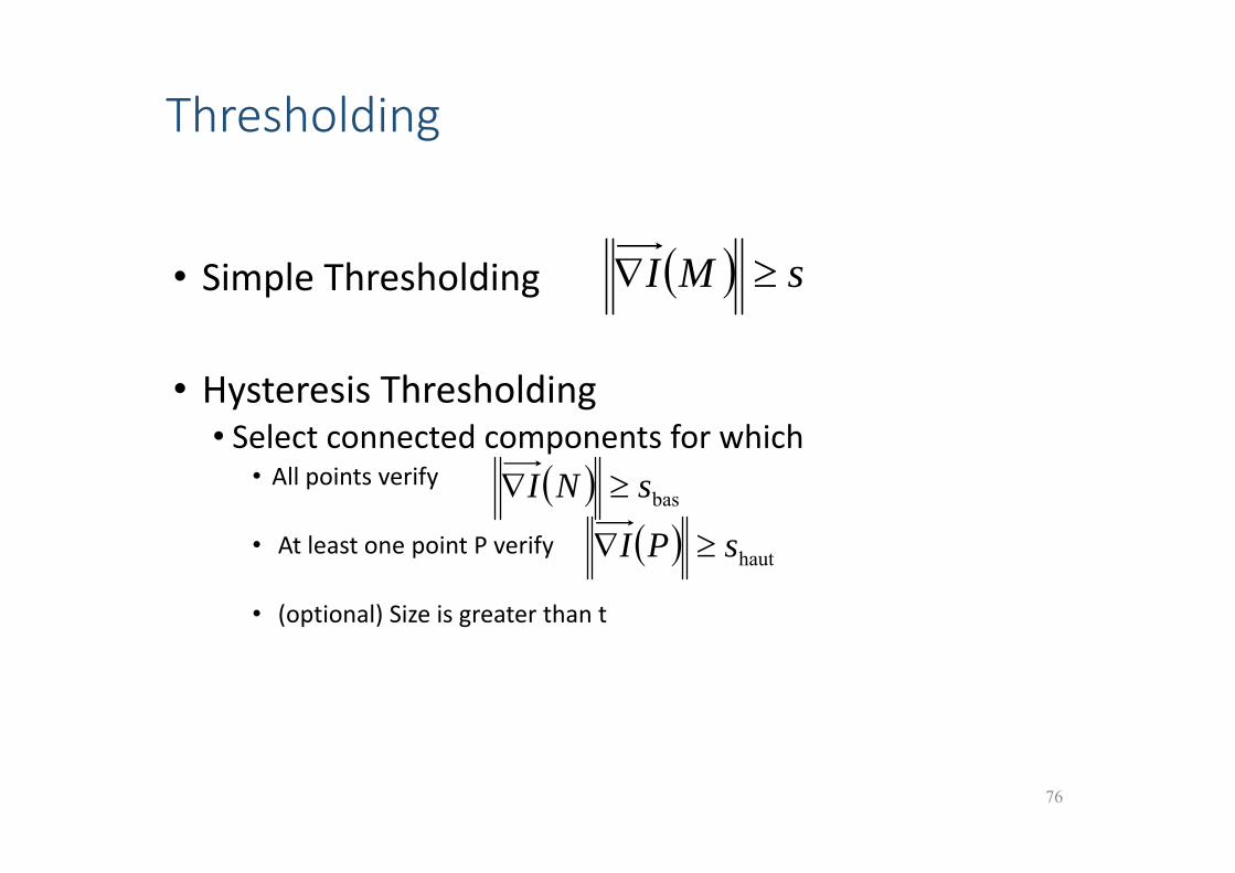
Thresholding
• Simple Thresholding
• Hysteresis Thresholding• Select connected components for which
• All points verify
• At least one point P verify
• (optional) Size is greater than t
76
sMI
bassNI
hautsPI
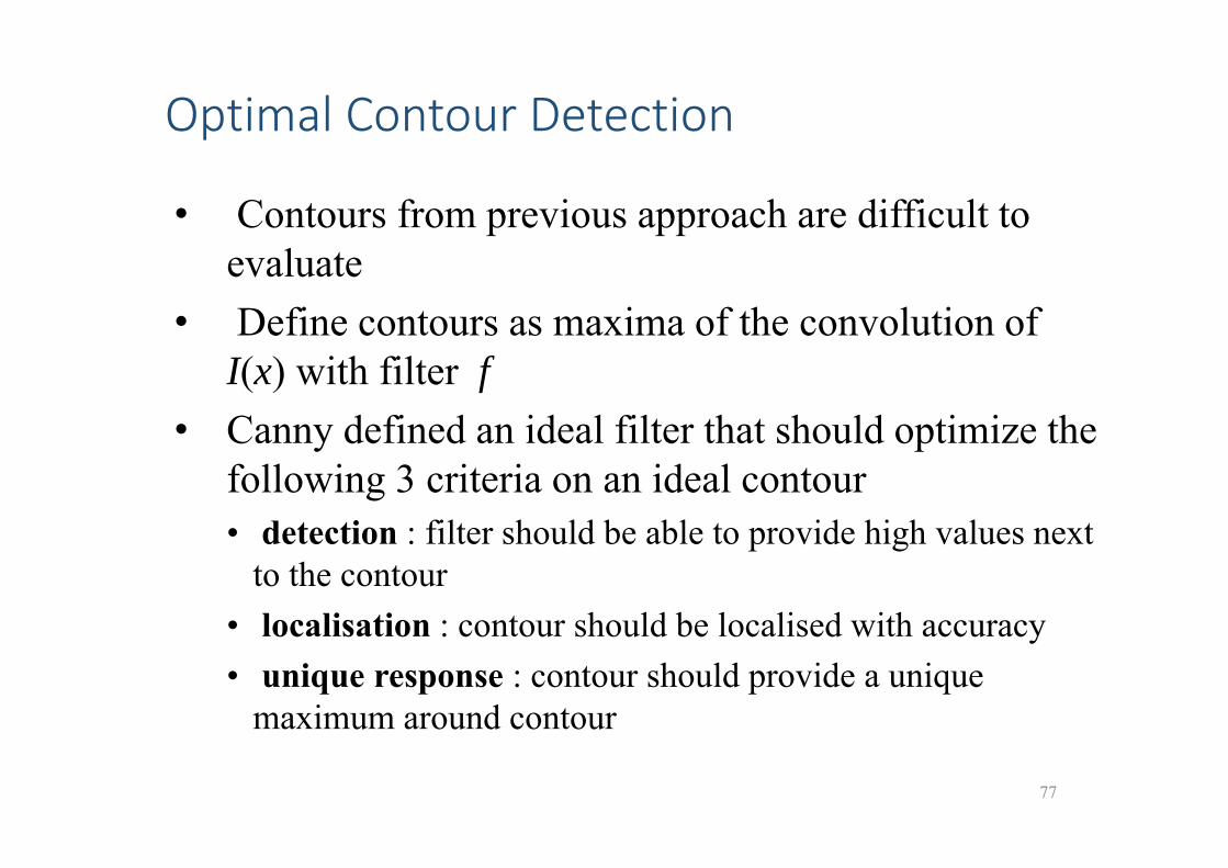
Optimal Contour Detection
77
• Contours from previous approach are difficult to evaluate
• Define contours as maxima of the convolution of I(x) with filter f
• Canny defined an ideal filter that should optimize the following 3 criteria on an ideal contour• detection : filter should be able to provide high values next
to the contour • localisation : contour should be localised with accuracy• unique response : contour should provide a unique
maximum around contour
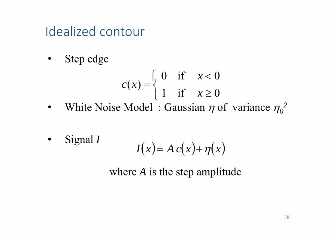
Idealized contour
78
• Step edge
• White Noise Model : Gaussian of variance 02
• Signal I
where A is the step amplitude
0if1 0if0
)(xx
xc
xxcAxI
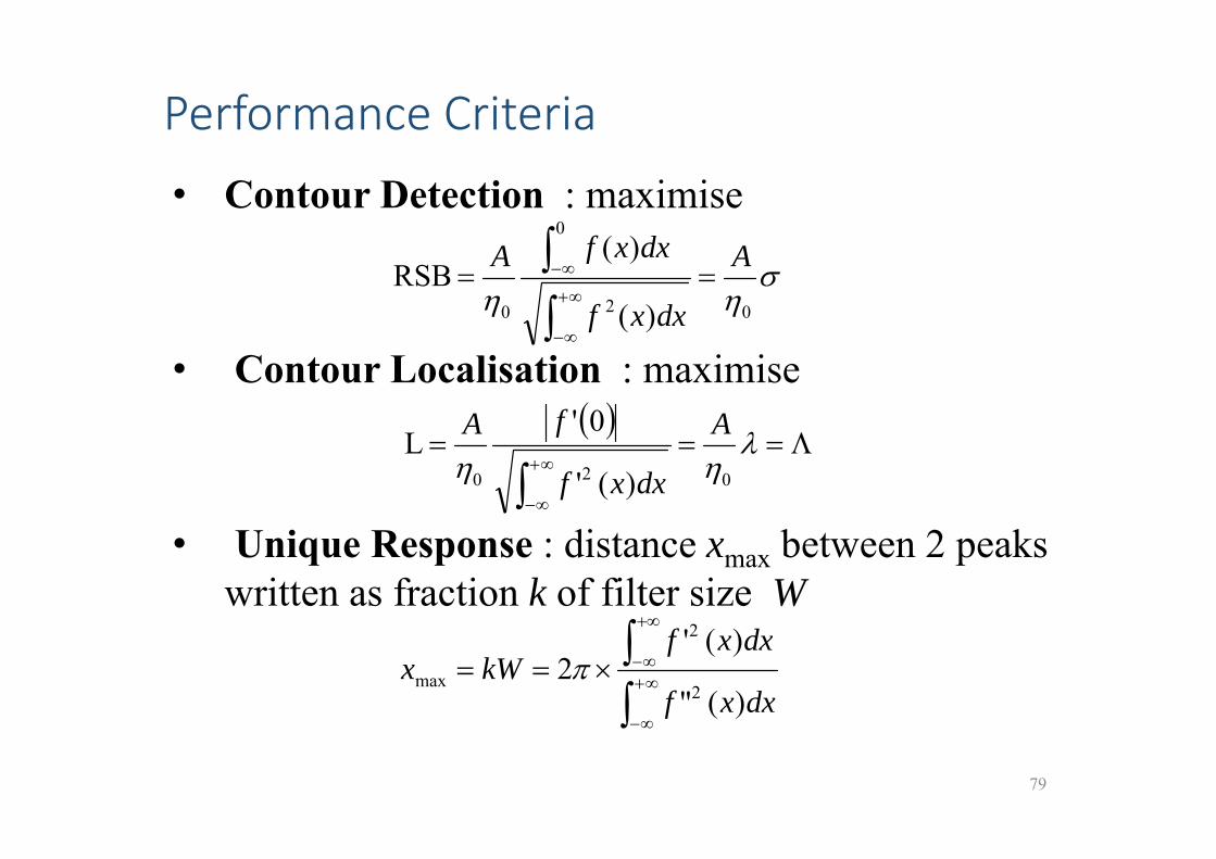
Performance Criteria
79
• Contour Detection : maximise
• Contour Localisation : maximise
• Unique Response : distance xmax between 2 peakswritten as fraction k of filter size W
02
0
0 )(
)( RSB A
dxxf
dxxfA
020 )('
0' L A
dxxf
fA
dxxf
dxxfkWx
)("
)('2
2
2
max
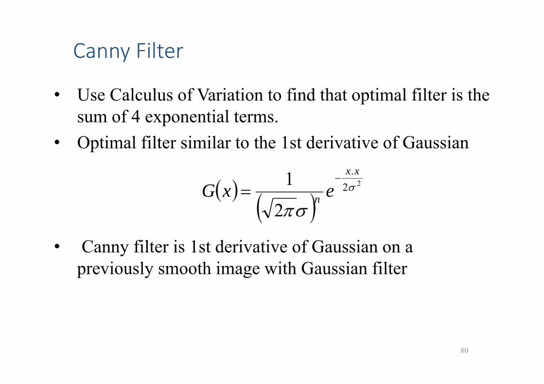
Canny Filter
80
• Use Calculus of Variation to find that optimal filter is the sum of 4 exponential terms.
• Optimal filter similar to the 1st derivative of Gaussian
• Canny filter is 1st derivative of Gaussian on a previously smooth image with Gaussian filter
22
.
2
1
xx
n exG
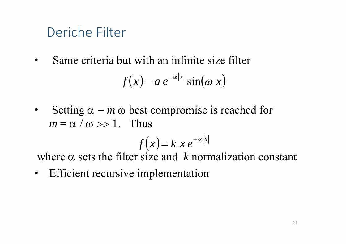
Deriche Filter
81
• Same criteria but with an infinite size filter
• Setting = m best compromise is reached for m = / 1. Thus
where sets the filter size and k normalization constant • Efficient recursive implementation
xeaxf x sin
xexkxf

Contour Detection 2D / 3D
87
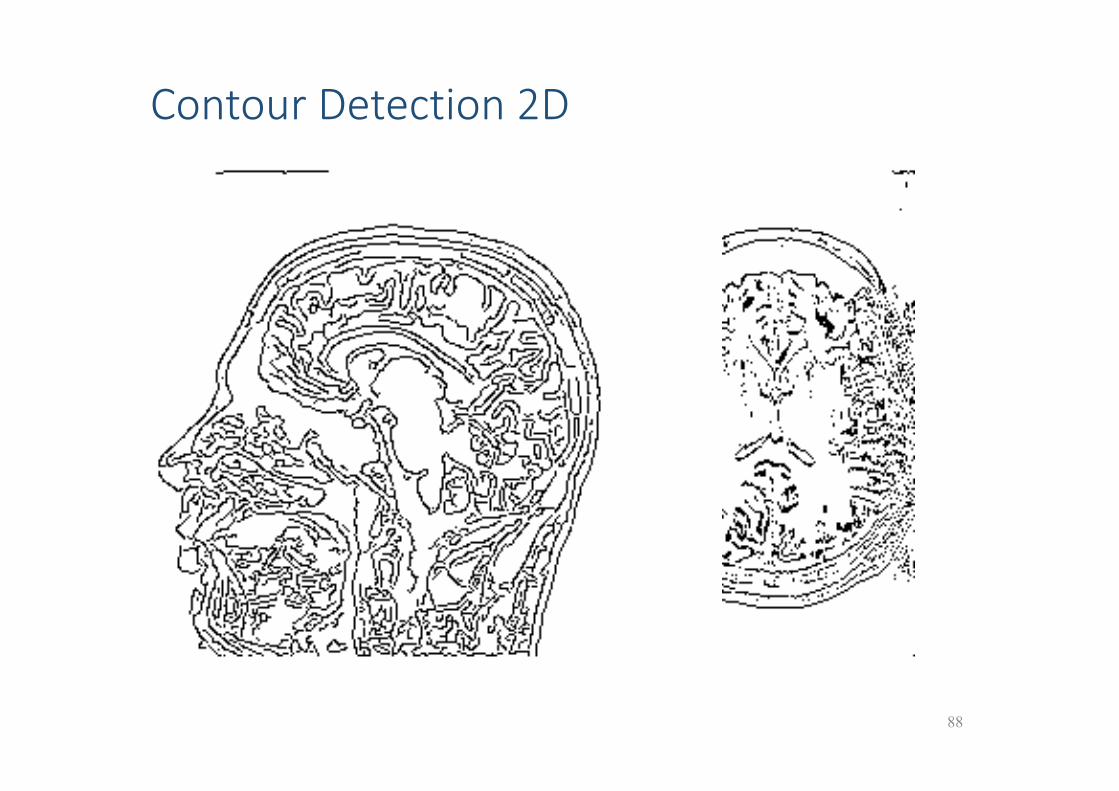
Contour Detection 2D
88
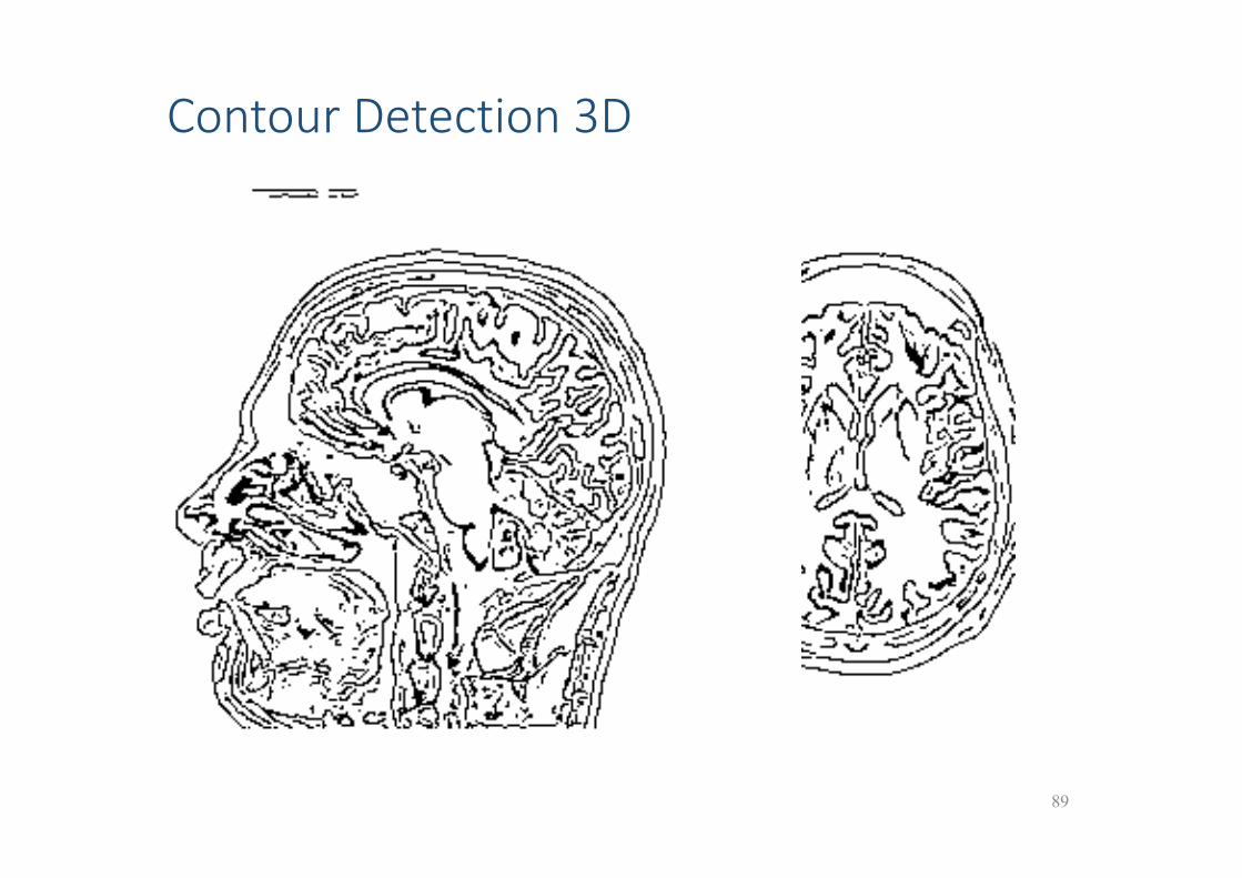
Contour Detection 3D
89
Segmentation
3 Mathematical Morphology
Overview
•Definitions of Neighborhood•Transformations on Binary Images
• Boolean• Hit or Miss• Erosion• Dilation
•Extension to Grey‐level Images
91
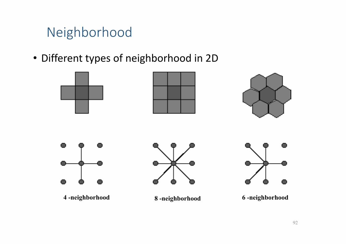
Neighborhood
• Different types of neighborhood in 2D
92
4 -neighborhood 8 -neighborhood 6 -neighborhood

Neighborhood
• Some generalizes to higher dimensions•Corresponds to a choice of metric norm
93
n
iii xyyxD
11 ),(
n
iii xyyxD
1
22 ),( iini
xyyxD ...1
max ),(
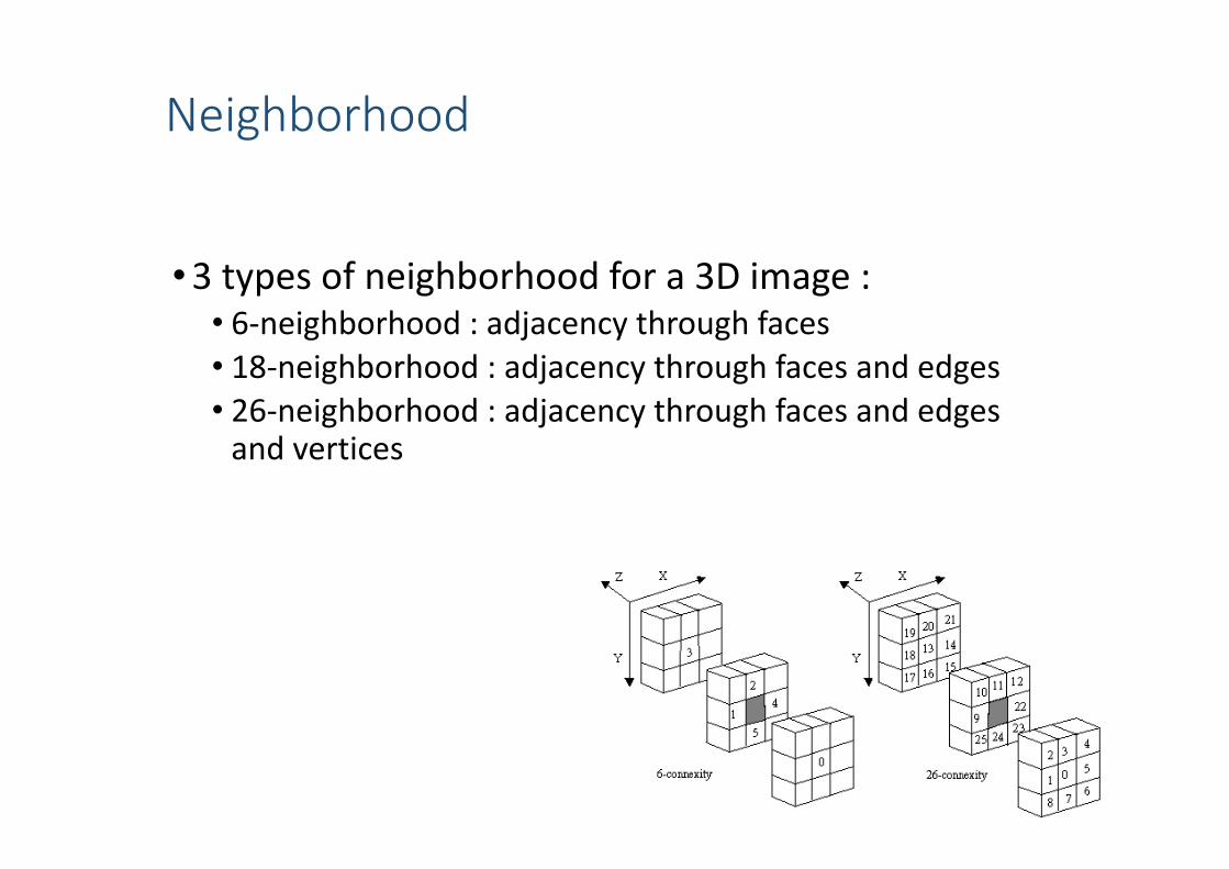
Neighborhood
•3 types of neighborhood for a 3D image :• 6‐neighborhood : adjacency through faces• 18‐neighborhood : adjacency through faces and edges• 26‐neighborhood : adjacency through faces and edges and vertices
94
Mathematical Morphology
•Technique to manipulate digital shapes• Unknown image • Known shape : structuring element
•Boolean operation between image & structuring element
, , , , , ...•See work by Serra, Schmitt, ...
95
Definitions (Binary)Ea Affine spaceEv Associated vector spaceI : Binary Image : K Ea {0,1}X : Foreground Object
X = {x K / I(x)=1}Xc : Background Object complementary of X with respect to Ea, B : structuring element = { b Ev } set of vectors = { x Ea / Ox = b} set of points
96

Definitions (Binary)
97

Boolean Operations• Union : X Y = { x / x X or x Y } • Intersection : X Y = { x / x X and x Y } • Inclusion : X Y x X x Y• Non symmetric difference
X \ Y = {x / x X and x Y}• Symmetric Difference
X \\ Y = { x / x ((XY)\(XY)) }• Complement
(Xc)E= { x / x E and x X }
98
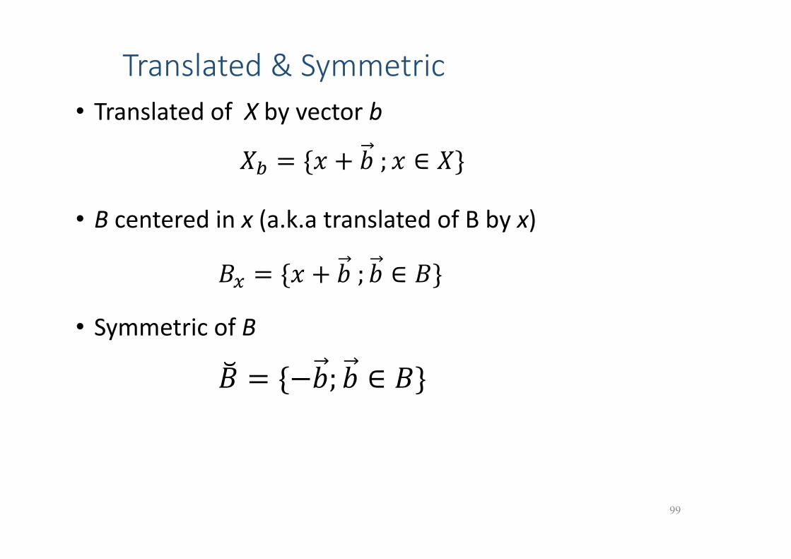
Translated & Symmetric• Translated of X by vector b
• B centered in x (a.k.a translated of B by x)
• Symmetric of B
99

Hit or miss transformation
• Partition of a structuring element BB = B1 B2 et B1 B2 =
• Hit or miss transformation of set XX B= { x / B1
x X et B2x Xc }
• x X B B1
x is in foreground and B2x is in background
B describe the local configuration of the background and foreground objects
100
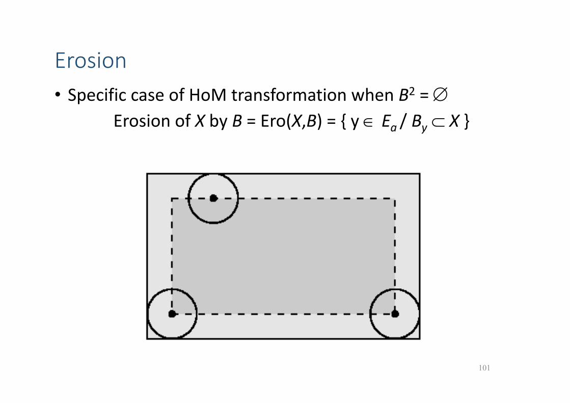
Erosion• Specific case of HoM transformation when B2 =
Erosion of X by B = Ero(X,B) = { y Ea / By X }
101
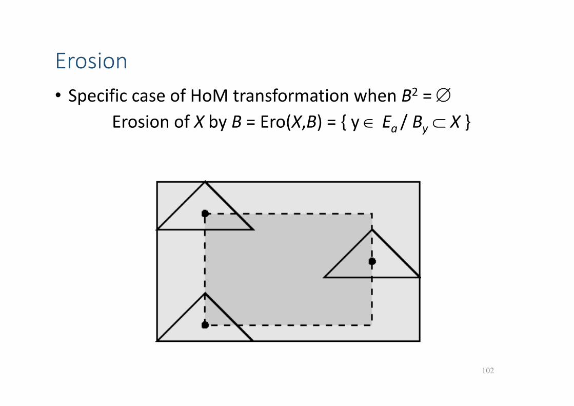
Erosion• Specific case of HoM transformation when B2 =
Erosion of X by B = Ero(X,B) = { y Ea / By X }
102
103
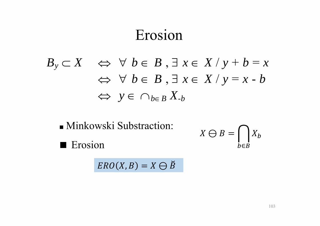
Erosion
By X b B , x X / y + b = x b B , x X / y = x - b y bB X-b
Minkowski Substraction:
Erosion⊖
∈
, ⊖

104
Erosion
4-structuring elementiterations = 2 iterations = 5
105
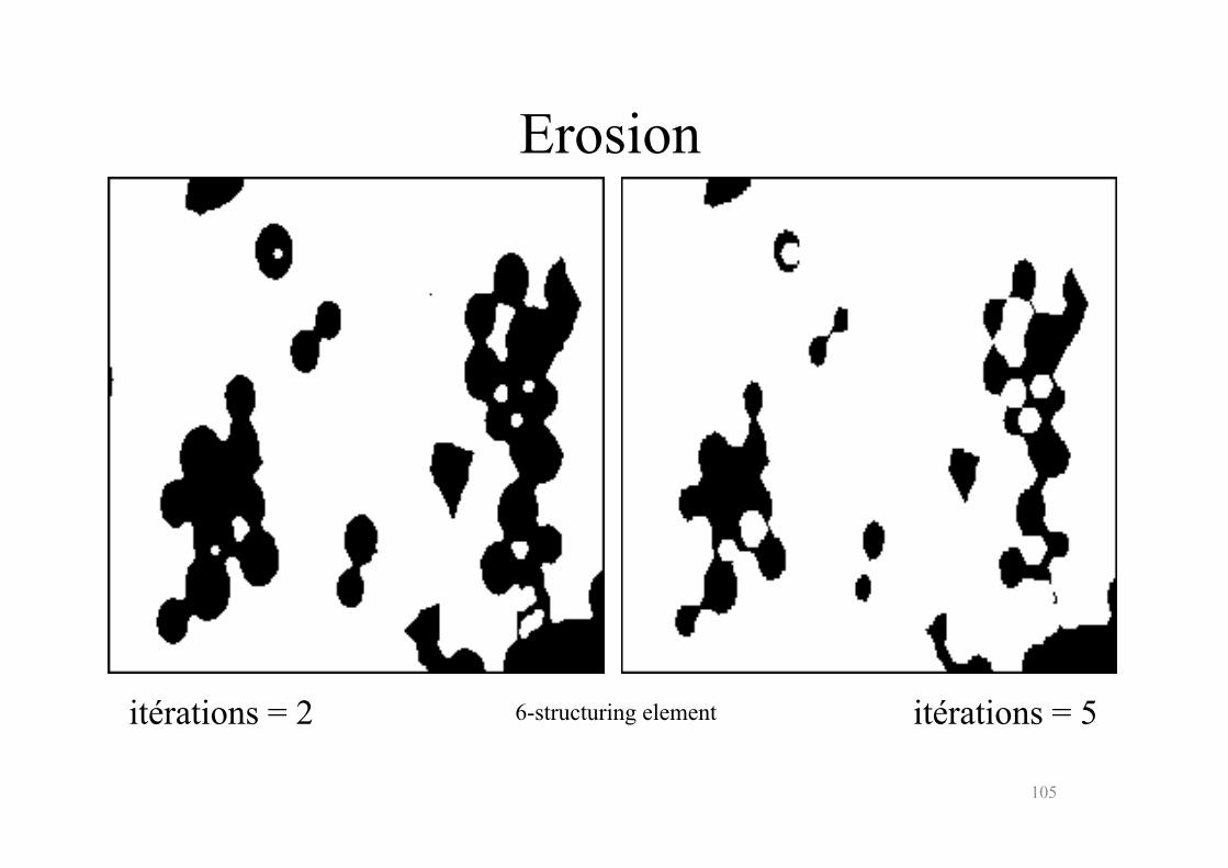
Erosion
6-structuring elementitérations = 2 itérations = 5

106
Erosion
8-structuring elementitérations = 2 itérations = 5
Dilation
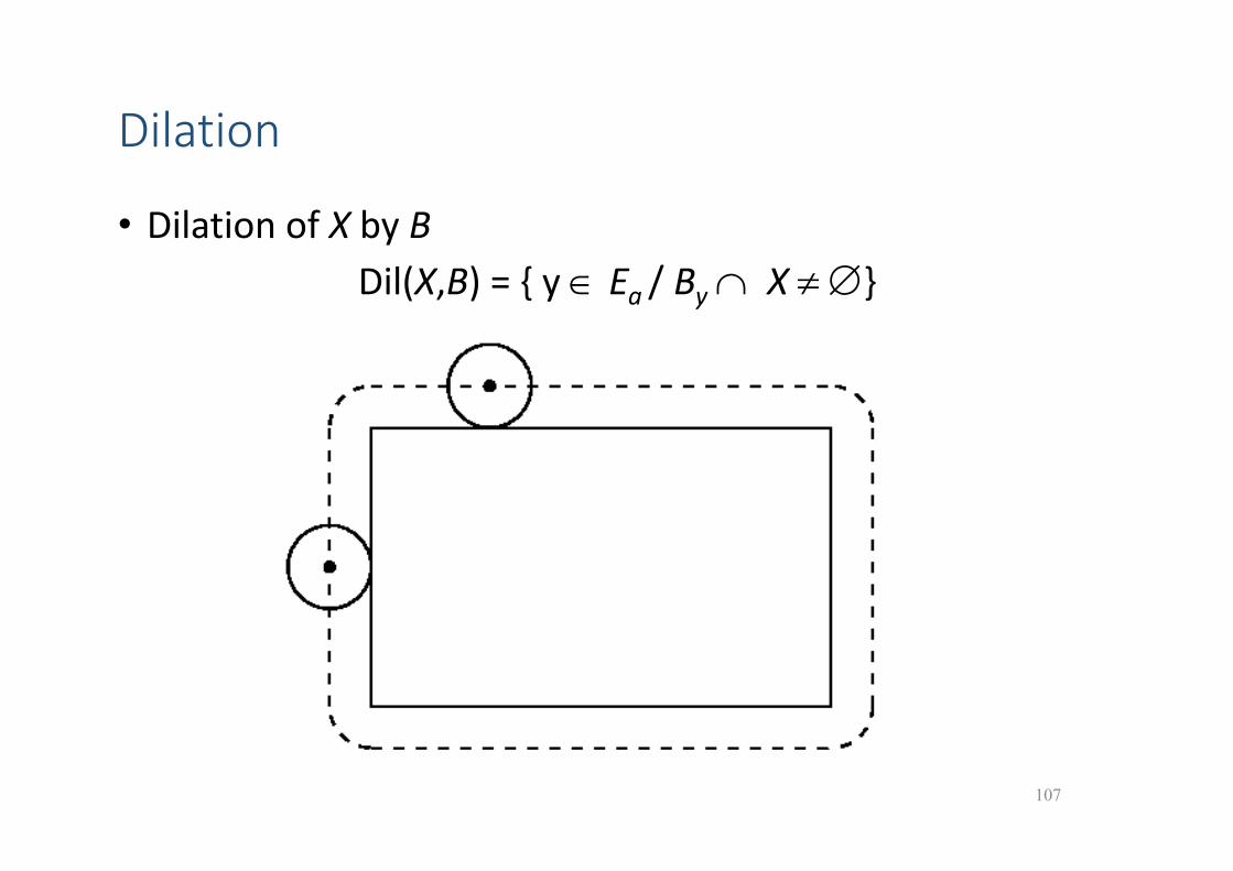
• Dilation of X by B Dil(X,B) = { y Ea / By X }
107
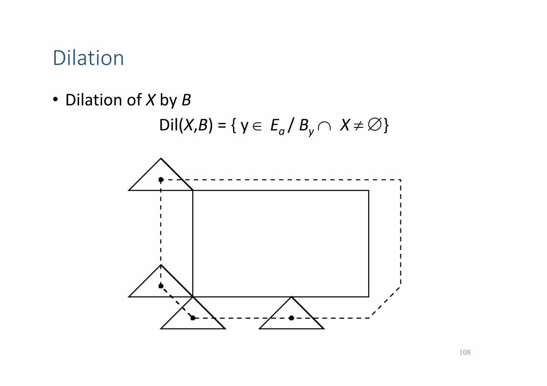
Dilation
• Dilation of X by BDil(X,B) = { y Ea / By X }
108

109
Dilation
By X b B , x X / y + b = x b B , x X / y = x - b y bB X-b
Minkowski Addition:
Dilatation⊕
∈
, ⊕
110
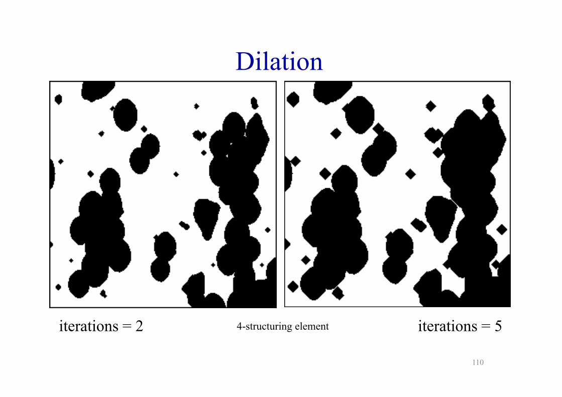
Dilation
iterations = 2 iterations = 54-structuring element
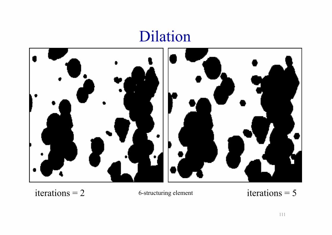
111
Dilation
6-structuring elementiterations = 2 iterations = 5
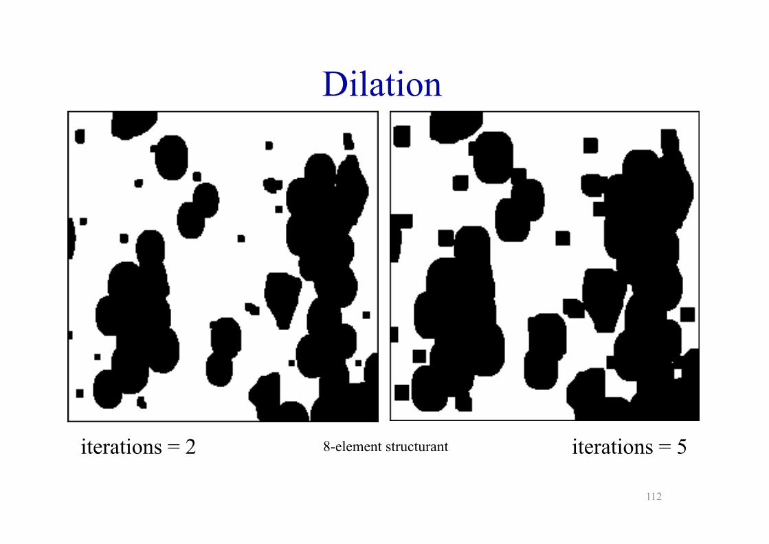
112
Dilation
8-element structurantiterations = 2 iterations = 5
113
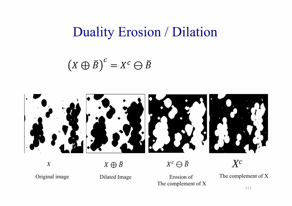
Duality Erosion / Dilation
X Xc⊕ ⊖
Original image Dilated Image Erosion of The complement of X
The complement of X

![Neural Discrete Representation Learningpapers.nips.cc/paper/7210-neural-discrete-representation-learning.pdf · variables [27]. Using discrete variables in deep learning has proven](https://img.pdfslide.net/doc/110x75/5f9fc45cad3f5378060015cb/neural-discrete-representation-variables-27-using-discrete-variables-in-deep.jpg)