Embed Size (px)
Citation preview

Medical Out-of-Pocket Expenses, Poverty, and the Uninsured∗
Kyle J. Caswell†and Brett O’Hara
SEHSD Working Paper 2010-17‡
U.S. Census BureauWashington, D.C.
December 29, 2010
Abstract
The National Academy of Sciences (NAS) Panel on Poverty and Family Assistance ar-gued that the current official U.S. poverty measure should be updated to capture changes inthe population’s healthcare costs and needs; families with sufficiently high medical out-of-pocket (MOOP) expenditures may be ‘poor’ even though they are not counted as such. Thisresearch offers three distinct advances toward achieving the NAS recommendations as theyconcern MOOP spending. Firstly, this paper uses the newly collected MOOP expendituredata from the CPS ASEC, and analyzes its quality vis-a-vis alternative sources. Secondly,poverty estimates that incorporate the MOOP spending data from the CPS ASEC are pro-duced in such a way as to be consistent with the NAS recommendations. These direct es-timates are an improvement over previous estimates, conditional on obtaining high-qualitydata, because modeling MOOP expenditures from other surveys is not needed. Third, thispaper investigates how the distribution of MOOP expenditures, and the poverty estimates,change when it is assumed that the uninsured have the spending patterns of the insured.The main results are: 1) the new MOOP expenditure data is high quality; 2) incorporat-ing observed MOOP expenditures increases the incidence of poverty across the populationby approximately two percentage points over the official measure; 3) counterfactual esti-mates of non-premium MOOP expenditures for the uninsured does not significantly affectpoverty estimates; and 4) counterfactual estimates of premium MOOP expenditures for theuninsured exert significant upward pressure on the poverty rate.
∗This paper is released to inform interested parties of ongoing research and to encourage discussion of workin progress. Any views expressed on statistical and methodical issues are those of the authors and not necessarilythose of the U.S. Census Bureau.
†E-mail: [email protected] / Phone: 301 763 1271‡http://www.census.gov/hhes/povmeas/methodology/supplemental/research.
html
1

1 Introduction
Medical out-of-pocket (MOOP) spending may reach a non-trivial share of overall expenditures,especially for low-income families. Among insured families, on average, half of total MOOPspending is on health insurance premiums (Banthin et al., 2008). In some cases, health eventsmay result in high non-premium MOOP spending—regardless of health insurance coveragestatus. For example, researchers estimated that approximately half of all U.S. bankruptciesin 2001 involved medical debt and approximately 75 percent of the people affected had healthinsurance coverage at the onset of their illness (Himmelstein et al., 2005). Others have identifiedcorrelations with health events and significant wealth losses (Cook et al., 2010; Smith, 1999). Inshort, MOOP spending lowers family resources such that available income for food and shelterdecreases—namely, components used to measure poverty status.
Given this reality, the National Academy of Sciences Panel on Poverty and Family Assis-tance made several recommendations concerning the incorporation of MOOP spending into analternative measure of poverty (Citro and Michael, 1995). The NAS recommended approachis to include actual MOOP spending as a limitation on resources: total family income minustotal family MOOP spending, which is the numerator of a poverty rate. The fundamental ad-vantage of the NAS recommended approach is that the distribution of actual MOOP spendingis preserved. Nonetheless, others have argued that expected MOOP spending should be incor-porated into the poverty thresholds (i.e., the denominator of a poverty rate). The argument forincorporating expected MOOP spending in the threshold is that some families under-consumemedical services; in particular, people have unmet medical needs because, in part, they do nothave health insurance coverage (e.g., Banthin, 2004).
This research offers three general refinements to incorporate MOOP expenditures into thepoverty measure. Firstly, this work uses the newly added questions collected in the 2010 CurrentPopulation Survey Annual Social and Economic Supplement (CPS ASEC). These new ques-tions are designed to directly calculate the Supplemental Poverty Measure (SPM) and MOOPspending. This work investigates the quality of the new MOOP spending data vis-a-vis alter-native well-known and high-quality data sources. Secondly, the effect of incorporating the newMOOP spending data into the poverty estimates is investigated using the NAS recommenda-tion. That is, observed total family MOOP spending is subtracted from family income, and theofficial thresholds are used to measure the change in the incidence of poverty. This simple esti-mation offers an improvement over previous attempts that depended on model-based methods,conditional collecting high-quality MOOP expenditure data in the CPS ASEC.
The third and final component to this research incorporates the notion that some families
2

would (on average) have higher MOOP spending if they were less resource constrained, andinvestigates to what extent this constraint exerts downward pressure on poverty status. It is alsoan explicit research priority outlined by the Interagency Technical Working Group on Develop-ing a Supplemental Poverty Measure (U.S. Census Bureau, 2010). Based on the premise thatpeople with health insurance coverage are less constrained in consuming medical services, acounterfactual distribution of non-premium expenditures for the uninsured is estimated basedon their income and demographic characteristics. To investigate the robustness of the results,two methodologies are implemented: predictive mean matching, and propensity score match-ing. These counterfactual distributions are then subtracted from total family income to investi-gate how the poverty estimates are affected. As a last step, non-group premiums are imputedfor uninsured family units, and are added to the counterfactual non-premium MOOP spendingdistributions for the uninsured, in order to investigate how both adjustments affect the povertyestimates. Overall, this effort highlights the potential impact on the SPM if the uninsured pop-ulation’s MOOP spending was more like that of the insured.
Results indicate that the newly collected MOOP spending data in the 2010 CPS ASECdata are high quality, yet some (minor) areas of data improvement are identified, and remediesimplemented. After incorporating the new MOOP spending data, the incidence of people inpoverty increases from 14.3 percent in the official measure to 16.4 percent in the alternativemeasure of poverty (that only accounts for MOOP spending). The counterfactual distributionsof non-premium MOOP spending for the uninsured did not significantly change the povertyrate, compared to the estimates using the uninsured’s observed non-premium MOOP spending.However, the (modeled) non-group premium expenditures for the uninsured exert significantupward pressure on the poverty rate among the uninsured and the overall population.
2 Previous Research: the CPS, MOOP, Poverty, and MOOP Spending Adjustments forthe Uninsured
Banthin et al. (2000) investigates the effects of including (mean and median) MOOP expendi-tures (by family type) to the poverty thresholds using the 2000 Current Population Survey (CPS;reference year 1999), Consumer Expenditure Survey (CE), and the 1996 Medical ExpenditurePanel Survey (MEPS)—MOOP expenses are estimated using the latter two surveys. The authorsexplicitly add a “standard, unsubsidized insurance package” to non-premium MOOP expensesreported by uninsured families (Banthin et al., 2000, p.9).1 Specifically, the authors’ derivecounterfactual premium expenditures based on employer-based premium prices, yet include es-
1Note that the 1996 MEPS did not collect out-of-pocket premium expenses for respondents receiving healthinsurance from their current employer/union, which changed in post 1996 surveys.
3
timates of the employer contribution. Without the uninsured adjustment, including MOOP intothe thresholds increases the estimate of individuals in poverty by approximately 1.7-2.9 percent-age points over the official measure, depending on data source and method (Banthin et al., 2000,table 6). The additional adjustment for uninsured premium spending increases the poverty esti-mates by approximately 3.1-3.7 percentage points over the official measurement, depending onthe method implemented.
Betson (2001) is an early attempt to model total MOOP expenditure data using the CE.The model incorporates statistical matching (random assignment) to create synthetic MOOPexpenditure data for CPS ASEC respondents. The sample is separate for families headed bynon-elderly versus elderly adults. MOOP spending is modeled at the family level in two stepsto account for zero spending and non-zero spending. Since this model has been used extensivelyfor imputing MOOP spending values to CPS respondents.
Short (2001), in part, incorporates total family MOOP spending into the poverty estimatesfor the 1999 population by 1) using the Betson model that matches MOOP spending values toCPS respondents and subtracts it from family income (MOOP Subtracted from Income; MSI),and 2) developing new poverty thresholds (MOOP in the Thresholds; MIT). Short simultane-ously includes adjustments for work related expenses, housing subsidies, and geographic adjust-ments for living expenses. Given these additional (non-MOOP spending related) adjustments,a direct investigation of how incorporating only MOOP expenses affect the official poverty es-timate unclear. Nonetheless, the MOOP adjustment makes a large contribution relative to theothers. Using the Betson model, the poverty rate among all people increased by 0.2 percentagepoints using the MSI method and by 0.8 percentage points using the MIT method.
Although widely used, the Betson model has been criticized on many grounds. For example,O’Hara and Doyle (2001) suggest that modeling MOOP spending based on individual charac-teristics is more appropriate than family-level characteristics, and that predictive mean match-ing may be a more appropriate matching method. They investigate the effect of incorporatingMOOP spending on estimated poverty rates using the SIPP, MEPS, and CE (reference period1996), and use several different methodologies—the Betson model, predictive mean match, anda special case of predictive mean matching—for creating synthetic MOOP spending for SIPPrespondents. They incorporate MOOP spending by subtracting total family MOOP spendingfrom total family income (i.e., MSI approach), and apply the official poverty thresholds. TheMOOP adjustment increases the estimated incidence of people in poverty by approximately 1.5to 1.9 percentage points over the official measurement across the entire population (O’Hara andDoyle, 2001, table 3), depending on the matching method and MOOP data source.
More recently, O’Donnell and Beard (2009) reaffirm that predictive mean matching is more
4

appropriate than random assignment, used in the Betson model. They also concluded that usingup-to-date data are essential for good estimates, compared to the Betson model which uses aCPI adjustment to the CE for imputation. Short (2010) incorporates the predictive mean match-ing model in O’Donnell and Beard (2009) for MOOP spending and applied it to the 2008 CPSASEC (reference year 2007). That research incorporates several adjustments in response to theMeasuring American Poverty Act. The MOOP spending adjustment effect on the poverty esti-mate cannot be isolated because the adjustments on the alternative poverty estimates were donesimultaneously, as in Short (2001). However, MOOP spending is one of the largest componentsto the new adjustment. When all adjustments are taken into account, the poverty rate increasesby 2.8 percentage points over the official measure (Short, 2001, table 7).
3 Data Sources
To evaluate the quality of the newly collected MOOP spending data in the Current PopulationSurvey Annual Social and Economic Supplement (CPS ASEC), it is compared to well-knownhigh-quality alternatives. Specifically, the CPS ASEC is benchmarked to the most recentlyavailable information in the Medical Expenditure Panel Survey (MEPS), and the Survey ofIncome and Program Participation (SIPP), Medical Spending and Utilization Module. Thereare similarities and differences across these three surveys, which lead to predictable differencesin MOOP spending estimates (discussed below). All monetary values in the SIPP and theMEPS have been converted to constant 2009 US dollars by applying the CPI all items (series id:CUUR0000AA0) and the CPI Medical Care index (series id: CUUR0000SAM) to the incomeand MOOP spending data, respectively (Bureau of Labor Statistics, 2010).2
3.1 The Current Population Survey, Annual Social and Economic Supplement, 2010
The Annual Social and Economic Supplement to the Current Population Survey (CPS ASEC)is a nationally representative survey of the civilian, non-institutionalized U.S. population. TheCPS ASEC is mostly administered in March although some data are collected in February andApril. This paper uses the data collected in 2010, and the corresponding reference period forthe respondents is from January to December of 2009. Approximately 77,000 households were
2The estimates in this paper (which may be shown in the text, figures, and tables) are based on responses fromsamples of the population and may be different from actual values because of sampling variability or other factors.As a result, apparent differences between the estimates for two or more groups may not be statistically significant.All comparative statements have undergone statistical testing and are significant at the 90 percent confidenceinterval unless otherwise noted. Standard errors were calculated using each survey’s appropriate method: replicateweights for the CPS (U.S. Census Bureau, 2009b) and the SIPP (U.S. Census Bureau, 2009a), and using the surveydesign (PSUs and strata) for the MEPS (Machlin et al., 2005).
5

interviewed (approximately 210,000 individuals, belonging to almost 85,500 ‘families’).3 TheCPS ASEC is the official survey used for the national poverty and health insurance coverageestimates.
In 2010, the CPS ASEC began collecting MOOP expenditure data in order to integrate theseexpenses into the SPM. MOOP expenditure questions in the survey are general, and are capturedin three separate questions. Respondents eighteen years old and older are asked to report totalhealth insurance premium expenditures over the year, for all health insurance policies—privateand public—except Medicare Part B premiums. Two separate questions on total non-premiumMOOP expenditures (paid for by anyone in the household) are asked of respondents, dependingon whether they are older/younger than fifteen years old.4 No distinction is made for the typeof non-premium MOOP spending (e.g., doctor visit versus medical supplies). A final questionprobes whether any MOOP expenses (premium and/or non-premium) were, or will be, reim-bursed; and if so, how much.
Respondents in the CPS ASEC report their health insurance coverage status—private policy,Medicare, Medicaid, a form of Veterans’ coverage, or no coverage—as having been covered forat least one day in the reference period.5 From this information, three mutually exclusive cover-age categories are constructed. Individuals are defined as having ‘private insurance’ regardlessif they also have any form of public insurance. ‘Public insurance’ status is defined as having anyform of public insurance, and no private insurance, and ‘uninsured’ is the residual group. Simi-larly, three mutually exclusive groups are constructed to summarize family coverage. Privatelyinsured families are defined as those were at least one member has a private policy. Similarly,publicly insured families are those where at least one member has a public policy, and not aprivate policy. Uninsured families are those where all members report no insurance coverage.
3.2 The Survey of Income and Program Participation, Medical Spending and Utilization Mod-
ule
The Survey of Income and Program Participation (SIPP) is a multi-year panel survey with quar-terly interviews (i.e., waves) following the same individuals. The population in SIPP is repre-sentative of the civilian non-institutionalized U.S. population. This paper uses the SIPP 2004panel, wave six topical module, which includes the survey’s most recent medical expenditure
3The term ‘family’ used in this paper includes ‘single individuals’ and ‘secondary individuals’ and is thereforenot equivalent to the definition of family used in the CPS.
4The question for children under 15 years old is worded slightly differently than that for respondents aged 15+,yet it essentially collects the same information.
5Health insurance coverage estimates using the CPS ASEC are based on a reference period, and are not ‘pointin time’ estimates as derived from the American Community Survey (ACS) (see DeNavas-Walt et al., 2010).
6

information (discussed below). The reference period for wave six is October 2004 to January2005. Wave six of the 2004 panel interviewed approximately 49,500 households (95,000 indi-viduals in approximately 40,400 ‘families’).
The wave six topical module includes questions on the utilization of medical services, andadditional follow-up questions on medical expenses, for all family members. This format ofquestioning is intended to facilitate accurate reporting of non-premium MOOP spending. Likethe CPS ASEC, gross MOOP expenditures are collected separately for non-premium and pre-mium expenses. Respondents are given the opportunity to report if they were, or will be, re-imbursed for any of the MOOP expenses; and if so, how much. Total net MOOP spending iscalculated by adding gross premium and non-premium expenses, less reimbursements. Finally,MOOP expenditures are reported for the previous twelve months.
Health insurance coverage information in the SIPP is collected for each month of a givenquarter. Respondents are asked if they were covered, by insurance type, for at least one day ofa given month. In an effort to be as consistent as possible with the CPS ASEC, three mutuallyexclusive health insurance coverage indicators for individuals and families are created in thesame way as described in the CPS ASEC (discussed above).
3.3 The Medical Expenditure Panel Survey
The Medical Expenditure Panel Survey (MEPS) is a two-year rotating panel, with five equallyspaced interview collection periods, and it is a nationally representative sample of the civilian,non-institutionalized population. The survey collects detailed information on medical care uti-lization and expenditures by source of payment, and is considered one of the highest qualityhousehold surveys collecting MOOP expenditures (Cohen et al., 2009). Cross-sections of the2007 MEPS Household Component (MEPS-HC) data are used. The data cover the referenceperiod of January to December 2007 and is constructed from rounds three, four, and five ofpanel 11 and rounds one, two, and three of panel 12.6 The final sample includes approximately29,000 individuals, or about 12,000 CPS-like ‘families.’7
Non-premium MOOP expenditures in the MEPS is collected at the event level (e.g., doctorvisit), and is consequently able to distinguish spending by type of service.8 In addition to beingable to study types of non-premium MOOP spending, the data includes a large range of “small”(e.g., less-than $100) spending amounts. Similarly, out-of-pocket health insurance premium
6A round is the same concept as a wave in SIPP.7In the MEPS it is possible to redefine families using the same definition as the CPS. Weights are also provided
for each family definition, and this analysis makes use of those weights.8The MEPS non-premium MOOP spending categories are: office- and hospital-based care, home health care,
dental services, vision aids, and prescribed medicines.
7

expenditures are collected for each policy member-policy-round. Premium information in theMEPS is limited to spending to private health insurance policies, versus both private and publicpolicies combined.
Health insurance coverage information in the MEPS is also refined. At each round of in-terviewing, respondents report their coverage status, by type, for each month; i.e., monthlyestimates are available for the entire year. The annual summary of insurance status indicatorsis available on the public use file and they are constructed from the monthly coverage infor-mation.9 From this information, three mutually exclusive groups are constructed—privatelyinsured, publicly insured and not privately insured, and uninsured—for individuals and familiesin the same way as discussed above for the CPS ASEC and the SIPP.
3.4 Pertinent Conceptual Differences across the CPS ASEC, the SIPP, and the MEPS
3.4.1 Reference Periods
The most obvious difference across the three samples is with respect to the reference periods ofdata collection. This is most relevant insofar as the distributions of MOOP spending may not bestable, even after accounting for inflation, between October 2004 (the earliest period of MOOPspending in the SIPP) to December 2009 (the latest month for the CPS ASEC).
The economic crisis beginning in 2007, and ensuing rising unemployment, was accompa-nied by 1) an increase in the (population) uninsured rate from 2008 to 2009; 2) a significantchange the composition of medical insurance coverage—private coverage decreasing and pub-lic coverage increasing (DeNavas-Walt et al., 2010), and 3) possibly reduced consumption ofroutine medical treatment (Lusardi et al., 2010; Wall Street Journal, 2010), and likely reducedspending on medical services and equipment than before the recession. Given these changes,it is anticipated that the SIPP MOOP spending distributions may be different from that in theMEPS, and the CPS ASEC due to the different reference periods.
3.4.2 Premium & Non-Premium MOOP Spending
A fundamental and important distinction between the MEPS and the other two surveys is howthe former collects MOOP spending. Non-premium spending in the MEPS is collected at theevent level versus one summary question for all aggregated non-premium spending. It is antici-pated that the MEPS data, with its more refined method, will gather more accurate estimates—especially for “small” spending—compared to the CPS ASEC and the SIPP. Similarly, the
9For example, if an individual had Medicare for at least one day of one month over the entire year, the annualsummary indicator for Medicaid equals one.
8

MEPS premium expenses are collected for each policy member-policy-round versus a sum-mary question that asks about expenses on all policies combined. The likely outcome will bethe collection of more accurate data on private premium expenditures.
Another substantive difference between the MEPS and the CPS ASEC/SIPP is with respectto premium expenditures. The MEPS only collects MOOP premium spending on private healthinsurance policies versus both private and public policies combined. Therefore it is anticipatedthat the largest discrepancies in measured premium spending will be among the elderly, who aremostly covered by Medicare, and typically have their premiums deducted from their monthlySocial Security Retirement benefit. In other words, total premium spending measured in theMEPS among the elderly may be consistently lower than that measured in the SIPP and possiblythe CPS ASEC if respondents report Part B premiums.
Finally, the components of total MOOP spending—premium and non-premium—in the CPSASEC, and the SIPP, is reported gross of reimbursements. Respondents are then given theopportunity to indicate whether they will be reimbursed for any of the given expenses (premiumand/or non-premium); and if so, how much. Total net MOOP spending estimates are obtainedby subtracting the reported reimbursements. It is therefore not possible to achieve net premiumand non-premium expenditure estimates.10 Therefore, this difference may have the effect ofinflating the SIPP figures with respect to the MEPS.
4 Methodology
4.1 Direct MOOP Spending Estimates & Poverty
Each survey is analyzed to identify the differences/similarities in the unconditional distributionsof MOOP expenditures including the total, premium, and non-premium spending. The unad-justed mean and median statistics of MOOP spending by commonly studied demographic in-formation is reported. Individual- and family-level statistics are of interest insofar as the formermay produce differences in the latter. Family-level statistics are of primary interest, as ‘poverty’is defined at the family-level. Kernel density estimates of MOOP spending for each survey areinvestigated to detect differences across the entire distribution. Finally, direct poverty estimatesusing the new data are presented by subtracting the actual total family MOOP spending fromtotal family income, per the NAS recommendations.
10Reimbursements collected in the 2010 CPS ASEC were positive for about 0.5 percent of the population, andmostly were greater than the total amount of MOOP spending in these cases. Therefore, this paper does not makeuse of the reimbursement data in the 2010 CPS ASEC, as its quality is questionable.
9

4.2 Counterfactual Estimates: Uninsured Non-Premium Spending Adjustment
The second component of this paper addresses the questions: 1) What would the distributionof non-premium MOOP spending among uninsured children and non-elderly adults look like ifthey had the spending patterns of their insured counterparts?; and 2) If the uninsured had theformer distribution of MOOP spending, how would the incidence of poverty change, if at all?For robustness checking, two separate methodologies are implemented to estimate a counterfac-tual distribution of non-premium MOOP spending for the uninsured: propensity score matchingand predictive mean matching. Finally, this analysis is limited to the non-elderly population asthe elderly are almost universally insured by Medicare.
4.2.1 Propensity Score Matching
Following the standard ‘propensity score matching’ (PSM) application proposed in Dehejia andWahba (2002), the first estimate is the ‘propensity score’ (i.e., the predicted probability) thatan individual has any form of health insurance, conditional on demographic information that iscorrelated with health insurance coverage. Separate model specifications are implemented forchildren versus non-elderly adults. This estimation takes the form of a standard logit model:
logit(p) ≡ log
(1
1− p
)= µ+ β′x (1)
where p is the probability that the individual respondent has (any form) of health insurance,Pr[Insured=1]; x is a vector of demographic characteristics correlated with health insurancestatus, which is different for children11 versus non-elderly adults;12 β is a vector of parameters tobe estimated; and µ is the intercept term corresponding to having any form of health insurance—
11Covariates for children aged 0-18 include: natural log of total CPS-family income; number of individuals inthe CPS family aged 0-18, 19-64, and 65+; highest educational attainment of all family members (less-than HighSchool Diploma, High School Diploma equivalent/Associates Degree, Bachelor’s Degree, Master’s/ProfessionalDegree or Ph.D.); Self-Reported Health Status (Excellent, Very Good, Good, Fair, or Poor); age (0, 5-9, 10-13, 14-18); sex, race/ethnicity (white non-Hispanic, black non-Hispanic, other non-Hispanic, and Hispanic); and Censusregion of residence (Northeast, Midwest, West, and South).
12Covariates for adults aged 19-64 include: natural log of total CPS-family income; number of individuals inthe CPS family aged 0-18, 19-64, and 65+; marital status (married versus not married); highest educational attain-ment (less-than High School Diploma, High School Diploma equivalent/Associates Degree, Bachelor’s Degree,Master’s/Professional Degree or Ph.D.); Self-Reported Health Status (Excellent, Very Good, Good, Fair, or Poor);reported disability (difficulty doing errands OR trouble dressing or bathing OR memory trouble OR trouble walk-ing/climbing stairs); age (19-24 reference group, 5 year interval dummies thereafter); sex; race/ethnicity (whitenon-Hispanic, black non-Hispanic, Other non-Hispanic, and Hispanic); Census region of residence (Northeast,Midwest, West, and South); employment status (employed, self-employed, unemployed, not in labor force, andfull time student); number of employees working for employer (<25, 25-99, 100-499, 500+); and occupationdummy for wholesale/retail trade.
10

public and/or private. Equation (1) can be re-written in terms of the propensity score as follows:
p =1
1 + eβ′x, (2)
where p and β are estimated via Maximum Likelihood using SAS.After estimating the propensity scores, the uninsured (pU ) are matched to the insured (pI)
using the SAS user-written algorithm ‘Greedy Match’ (Mayo Clinic, 2003), which is an appli-cation of one-to-one ‘case-control’ matching (discussed below). Finally, after the appropriatematches are made, the actual non-premium MOOP spending values of the matched insuredindividuals (‘controls’) are donated to their uninsured counterparts (‘cases’).
4.2.2 Predictive Mean Matching
This application of ‘predictive mean matching’ (PMM) closely follows the method initiallydeveloped in Rubin (1986) and Little (1988). In this work, child and non-elderly-adult non-premium MOOP spending are modeled as a function of known demographic controls, condi-
tional on being insured. Our model specification of choice, based on experimentation withalternative specifications, is a one-part Generalized Linear Model (GLM), with a log-link, andan assumed Poisson error term.13 Explicitly, the model takes the following form:
ln(E[s| Insured = 1]) = β′x (3)
where s is total non-premium MOOP spending in 2009 US dollars, β is a vector of parametersto be estimated, and x is a vector of demographic controls that are highly correlated with non-premium MOOP spending. The controls are defined in the same way as those in equation (1)for children and non-elderly adults, respectively.
Once the parameters have been estimated for the models that are restricted to insured non-elderly adults (βI
A) and insured children (βIC), the predicted values for the insured (sI) are
calculated, as well as for the uninsured (sU ), who were excluded from the fit of the model. Inother words, predicted values of MOOP spending are obtained for the insured and the unin-sured using the model parameters for the insured. The predicted mean values of the uninsured(‘cases’; sU ) are matched with those of the insured (‘controls’; sI) using the Greedy Matchalgorithm. Finally, the uninsured children and non-elderly adults (‘cases’) are given the actual
non-premium spending values associated with their (one-to-one) matched insured counterparts(‘controls’).
13The Poisson specification is based on a Park test, and closely follows standard applications in the literature formodeling MOOP expenditures (e.g., Buntin and Zaslavsky, 2004; Manning and Mullahy, 2001).
11

4.2.3 G Match Algorithm
Greedy Match, or gmatch, is a user written macro in the SAS programming language that per-forms ‘case-control’ matching using the ‘greedy’ algorithm (Bergstralh and Kosanke, 1995).A given case is matched with the closest control—in this case, the minimum difference be-tween propensity scores/predicted means of the uninsured (cases; U) and the insured (controls;I). More formally, for a each case i ∈ U , the minimum distance (i.e., match) between thepropensity score (or predicted mean) among all possible matches j ∈ I in the control group iscalculated as
∀i ∈ U ∧ j ∈ I : min{D},
where D is a vector if distances for each case and potential control, and the calculated distancefor a given case i and control j in vector D is simply expressed as
Di,j = |XUi −XI
j |.
In this application we perform one-to-one case-control matching and it is equivalent to ‘nearestneighbor’ matching. Once a match is made, the process continues with the next remaining (i.e.,unmatched) case and the remaining controls. This algorithm is appropriately named “greedy,” asonce it finds a match, that match is never broken. It is considered the best among the remainingpossible matches, independent of the possible impact on potential future matches.14
4.3 Premium Expenditures and the Uninsured
The third component of this paper investigates: 1) What the distribution of premium expendi-tures would be for uninsured ‘benefit units’ (discussed below), if they were assigned (modeled)premium values reflecting current average prices within the non-group (i.e., direct purchase)health insurance market?; and 2) How would this premium adjustment, together with the non-premium adjustment (section 4.2), further affect the poverty estimations? Premium assignmentsare model-based imputations (discussed below). A ‘benefit unit’ is defined here as a group ofindividuals that are on—or would be on, in the case of the uninsured—the same non-grouphealth insurance policy. Possible benefit unit structures created for the uninsured include singleperson units, spouses without children, single adults with children, and spouses with children.
First, non-group health insurance premiums are modeled via Weighted Least Squares (WLS)for non-elderly policyholders, and respective beneficiaries, using the CPS ASEC data.15 Fol-
14For further reading on the greedy match algorithm, and competing matching algorithms, see Rosenbaum(1989) and the references therein.
15The sub-sample for this exercise is limited to non-group non-elderly policyholders who report non-zero pre-
12
lowing typical insurance policy structure, two models are estimated based on whether the policyis a single (i.e., non-family) or family policy. Covariates included in each respective model areintended to capture common underwriting practices—namely, age, health, and the number ofpeople on a given policy (America’s Health Insurance Plans, 2009; Merlis, 2005; Monheit andCantor, 2004). The family model is specified as the following:
yi = Xiβ1 +Miβ2 +Hiβ3 + ϵi, (4)
where yi indicates total premium expenditures for (family policy) policyholder i; Xi is a vectorthat indicates the number of individuals included on the non-group policy in a given age group(0-18, 19-34, 35-39, 40-44, 45-49, 50-54, 55-59, 60-64); Mi is a vector indicating whetherthe policy holder is married; Hi is a vector indicating the number of individuals on the policyreporting “Fair” or “Poor” health; and ϵi is the error term.
The model for single (non-family) non-group policyholders is a special case of the specifi-cation above, where 1) the vector Xi collapses to dummy variables indicating whether policy-holder i’s age falls within a given age range (the reference age group is less-than 18), and 2) Mi
is omitted.16
Finally, ‘benefit units’ are constructed among the uninsured children and non-elderly adultsin the CPS ASEC. Using the parameter estimates from the models described above, the modelsare fit to the uninsured benefit units to obtain predicted non-group premium values (imputations)for the uninsured benefit units. Uninsured children with associated family income below (statespecific) income eligibility levels for Children’s regular Medicaid and children’s CHIP-fundedexpansions are excluded from this exercise (Kaiser Family Foundation, 2010).
5 Results
5.1 Direct Estimates
5.1.1 Demographic Information: 2010 CPS ASEC, 2007 MEPS, and 2004 SIPP
Table 1 reports nationally representative summary statistics of commonly constructed demo-graphic information—health insurance status, health, age, geography, education, and race/ethnicity—for individuals from the 2010 CPS ASEC, 2007 MEPS and 2004 SIPP (Wave 6). Among all
mium spending and no other form of health insurance. Edited (imputed) data is also excluded. A WLS model isused to impute premium values, and not a matching model, namely because the number of uninsured benefit units(‘cases’) far exceeds the number of non-group policies (‘controls’) for a typical PSM/PMM application.
16Based on experimentation with alternative specifications, we omit health status as it didn’t significantly con-tribute to the non-family model.
13
these categories, the most obvious difference in the estimates across surveys is for health in-surance status, which is anticipated (discussed in Section 3.4). For example, the percentage ofpeople in the CPS ASEC covered by a private health insurance policy (63.9 percent) is largerthan that reported in the MEPS (61.7 percent), yet smaller than that reported in the SIPP (71.5percent). The percentage of CPS ASEC respondents that report having public health insurancecoverage and no private coverage (19.4 percent) is lower than in the MEPS (20.6 percent), andhigher than in the SIPP (13.4 percent). Given these differences in the insurance coverage com-position, it is anticipated that direct MOOP spending estimates by group may also differ acrosssurveys.
Despite the aforementioned differences in health insurance coverage status, the remainingdemographic information in Table 1 is comparable in magnitude across all three surveys. Forexample, 5.7 percent of respondents fall into the Other race/ethnicity category (i.e., non-white,non-black, non-Hispanic) in the CPS ASEC, which is lower than in the MEPS (6.8 percent),and the SIPP (6.5 percent). Differences in the estimates across surveys for the remaining in-formation on health, age, geography, education, and race/ethnicity are smaller in magnitude,although statistically significant in the CPS-SIPP comparison, and generally insignificant forthe CPS-MEPS comparison.
Table 2 reports family characteristics as families are the relevant unit of analysis for the offi-cial poverty measure. Like the individual-level statistics, the largest difference across surveys isamong the insurance status estimates. For example, 68.4 percent of families in the CPS ASEChave at least one privately insured member, compared to 66.2 percent in the MEPS, and 77.5percent in the SIPP. Other differences in the estimates that stand out (in magnitude) includehealth (CPS versus SIPP only), family size (CPS versus SIPP only), having a bachelors degree,and ‘other non-Hispanic’ family members. CPS ASEC families are less likely to have someonewith a Bachelor’s degree (21.6 percent) compared to the MEPS (24.8 percent) or the SIPP (23.0percent). CPS ASEC families are less likely to have a non-black, non-white, non-Hispanicmember (5.7 percent) compared to the MEPS and the SIPP (both 7.3 percent). Despite thesestatistically significant differences, mostly in the CPS-SIPP comparison, the magnitude of the(significant) differences in estimates across surveys are small—especially when considering thedifferences in reference periods.
5.1.2 MOOP Spending: 2010 CPS ASEC, 2007 MEPS, and 2004 SIPP
Table 3 reports statistics on individual-level MOOP spending for all three surveys by components—premium spending and non-premium spending—as well total MOOP spending. All monetarystatistics are expressed in real 2009 US dollars. Total and non-premium MOOP spending es-
14

timates are reported for the entire population, while premium spending is restricted to ages 18years old and older.
Differences in the estimates of average total MOOP spending per person is not statisticallysignificant over the three different surveys (Table 3). Nonetheless, there are notable differencesacross surveys when investigating the entire distribution of spending. There are fewer peoplethat have zero total MOOP expenditures reported in the MEPS (19.8 percent) than the CPSASEC (35.9 percent) or the SIPP (34.5 percent). This difference is likely due to the fact thatthe MEPS collects non-premium MOOP expenditures at the event-level, as opposed to a singlesummary question as in the CPS ASEC and the SIPP (see Section 3.4).
Figure 1 graphs the weighted kernel density estimates of the (natural log of) total MOOPspending for the three surveys. The MEPS density estimate, the dash-dot line in Figure 1, hasa much fatter left tail, and crosses the CPS distribution at about 4.5; this estimate of ln(MOOP)is approximately $90.
Average premium spending ($) per person (aged 18+) is not statistically different acrossall three surveys, reported in Table 3; nor is the percent of people that report zero premiumspending in the CPS-SIPP comparison. However, the proportion of zero spending is higher inthe CPS compared to the SIPP, which most likely reflects the significant decrease in privateinsurance coverage over the different survey reference periods (table 1). These similaritiesare surprising in that: 1) the CPS ASEC and SIPP are gross measurements, while the MEPSfigures are net, and 2) the MEPS includes only premium expenditures on private insurancepolicies. This may reflect that CPS respondents are not reporting Medicare Part B premiums(as instructed), and that the reimbursement information collected in the SIPP is limited to asmall number of respondents.
Estimates of non-premium MOOP spending per person are not statistically different acrosssurveys (Table 3). However, there are stark differences in the proportion of reported spend-ing equal to zero ($0) across surveys: 42.2 percent (CPS ASEC), 23.4 percent (MEPS), and40.7 percent (SIPP). Differences in the components of total MOOP spending are also appar-ent when visually investigating the entire distributions, as shown in the kernel density graphseach distribution (premium and non-premium spending) in Figure 2. The major differences intotal MOOP spending across surveys lies with non-premium spending (left panel, Figure 2)—premium spending distributions are much more similar in shape and proportion of reported zero($0) values (left panel, Figure 2). For non-premium spending, graphed in the right panel of Fig-ure 2, the left tail of the distribution is much larger in the MEPS than the distributions graphedin the other two surveys.
Table 4 reports family-level statistics on per-capita family income, income to poverty ratios
15

(IPR), and MOOP spending. Estimates of average family income per member are similar acrosssurveys: $30,460 (CPS ASEC), $30,245 (MEPS; not statistically different from CPS estimate),and $29,659 (SIPP; statistically different from the CPS estimate). The percentage of familieswith an IPR less than 150 percent is 25.4 percent for the CPS ASEC compared to 23.5 percentMEPS; on this dimension, the CPS ASEC and the SIPP are not statistically different.
Family-level total MOOP spending estimates ($)—and its two subcomponents, premiumand non-premium spending—are not statistically different across the three surveys (Table 4).Differences across surveys are pronounced in the percentage of zero values, which stems fromdifferences in non-premium spending. In the CPS ASEC, 29.2 percent of families report zeronon-premium expenditures, compared to 9.3 percent in the MEPS, or 26.7 percent in the SIPP.As discussed above, this difference is mostly a result of the differences in survey design; i.e.,the MEPS collects spending at the event level whereas the CPS ASEC and the SIPP collectsspending at the aggregate level.
In short, there are noticeable differences in the distributions of MOOP expenditures in thenew CPS ASEC questions compared to the MEPS and the SIPP. Nonetheless, the MOOP spend-ing data collected in the CPS ASEC compares well with well-known high-quality sources, suchas the MEPS. This is encouraging, especially considering the much greater level of detail usedin collecting MOOP spending information in the MEPS versus the CPS ASEC and the SIPP.17
5.1.3 MOOP Spending Among the Insured & the Uninsured
It is important to emphasize that the distributions of (non-premium) MOOP spending are muchdifferent by insurance status. The uninsured population is younger, less educated, and morelikely to be non-white than the insured population. Given these differences, it is anticipatedthat non-premium MOOP expenditures among the uninsured are different than the insured. Forexample, average non-premium MOOP spending per person for the insured in the CPS ASEC is$696 (37.7 percent of respondents report zero spending) among the insured compared to $417(64.4 percent zeros) among the uninsured (not reported).
Given the demographic differences of the uninsured, compared to the insured, there are atleast two compelling arguments as to why the insured spend more on average than the unin-sured. One reason is that younger people tend to have better health. Given that the uninsuredare disproportionately young, this lends to lower spending. Another reason may be that the
17We also investigated the differences in total family-level MOOP spending over all three surveys, and the syn-thetic series created by the Betson model mentioned in section 2. The Betson model, for example, underestimatesaverage total family-level spending per family by approximately 34 percent, and is greater for families without anelderly member. Finally, the comparison of kernel density estimates reveal that the shape of the distribution of datacreated by the Betson model is much different than any of the empirical distributions studied here.
16

uninsured, on average, have relatively less resources (e.g., income and wealth), and may simplyforgo needed medical care and therefore spend less.
Figure 3 graphs kernel density estimates of (the natural log of) non-premium spending forthe non-elderly by insurance status, and clearly illustrates the differences in the distributions.In terms of the shape of the distributions among non-zero values, the uninsured distribution(dashed line) has (slightly) fatter tails, and appears to be shifted left compared to the insuredgroup (solid line). The other salient difference—not included in the density estimates—is theproportion of zero ($0) spending by insurance status: 32.7 percent for the insured comparedto 63.7 percent for the uninsured. In other words, differences in average spending per personare largely driven by the much larger proportion of uninsured respondents reporting zero non-premium MOOP spending.
5.2 Counterfactual MOOP Estimates and Poverty18
5.2.1 Uninsured Non-Premium MOOP Expenditure Adjustment & Poverty
Table 5 reports average non-premium MOOP spending by level of aggregation (individuals0-64 and families without elderly members), insurance status, and method of counterfactualadjustment among the uninsured—Propensity Score Match (PSM) and Predictive Mean Match(PMM).19 Average non-premium MOOP spending per person among the uninsured increases byover $100 per person after the PSM adjustment (from $415 to $535), which is in part due to a de-crease in zero spending values (64.5 percent to 45.7 percent). Qualitatively similar findings areseen for the PMM adjustment. Note that one large reason why the unconditional distributions,after the adjustment, do not match exactly by insurance status is because a disproportionatenumber of the uninsured are relatively young.
Average non-premium spending per non-elderly family, reported in Table 5, increases byapproximately $150 after the adjustment; $719 to $863 for the PSM adjustment and to $829for the PMM adjustment, which is largely due to a decrease in zero spending (57.8 percent to35.2 percent with the PSM adjustment and to 32.6 percent for the PMM adjustment). Figure 4graphs the kernel density estimates of the natural log of non-elderly family-level non-premiumspending for insured families, uninsured families, and uninsured families post PSM and PMM
18Model estimations used for the uninsured counterfactual MOOP spending adjustments are available to theinterested reader in Appendix A, and are not discussed here.
19Recall that ‘uninsured families’ are only those where all members are uninsured, and partially insured fami-lies are defined as insured. Therefore the uninsured adjustment for non-premium spending also affects spendingestimates among (partially) insured families. Finally, families with at least one member age 65+, and one less-than65, are excluded in the tables/figures, and therefore do not reflect the entire universe of individuals who received anon-premium MOOP adjustment.
17

adjustment. Here it is clear that the distributions at the family-level are very different by in-surance status, and that the PSM and PMM adjustments result in qualitatively very similardistributions. The distribution of insured family spending is to the right of uninsured families,reflecting greater spending, and the adjustment for uninsured families’ pulls in the right tailslightly—all while increasing the number of positive spending families.
Table 6 reports poverty estimates for individuals and families, and for several different pop-ulations of interest, excluding and including MOOP spending, and the counterfactual estimatesfor the uninsured. As published in DeNavas-Walt et al. (2010), the official estimate of the per-centage of people in poverty in 2009 (for the entire population) is 14.3 percent (shown in column1). Incorporating MOOP expenditures increases the estimate to 16.4 percent (shown in column2). This is a statistically significant increase of 2.03 percentage points (column 5). Similarincreases in the poverty rate are estimated among children (20.6 to 22.5 percent), non-elderlyadults (12.8 to 14.4 percent), and the non-elderly (15.1 to 16.8 percent).
Accounting for MOOP expenditures at the family level, the poverty rate increases. Amongall families, 15.6 percent are estimated as being in poverty using the official poverty measure(Table 6, column 1), which increases to 17.9 percent after incorporating MOOP spending. Fam-ilies without an elderly member experience a smaller increase (17.2 to 18.8 percent), yet theincidence is higher for these families compared to families with an elderly member (not re-ported). Finally, there is no statistically significant increase in the estimated poverty rate afterincorporating MOOP expenditures among uninsured families without an elderly member. Thislack of increase can be explained by the fact that MOOP spending is significantly lower for theuninsured compared to the insured.
Columns (3) and (4) of Table 6 report the poverty estimates after incorporating the non-premium MOOP adjustment for the uninsured using PSM and PMM methods, respectively.Compared to the direct poverty estimates which include MOOP spending in column (2), thepoverty estimates after the uninsured adjustment do not significantly change (columns 6 and 7).The (raw and statistically insignificant) increase over these three groups falls in the range ofapproximately one-fourth to two-thirds of a percentage point (columns 6 and 7).
It is surprising that the non-premium MOOP spending adjustment does not have a largereffect on the estimated poverty rate. However, this is most likely because the uninsured are(mostly) young, and their matched insured counterparts (i.e., ‘controls’) have similar attributes—including low non-premium MOOP spending. Said differently, there are few families whoseestimated change in non-premium MOOP spending—on average, an increase of $100 per unin-sured person (Table 5)—positions them in poverty.
18

5.2.2 Uninsured Premium MOOP Expenditure Adjustment & Poverty
Table 7 reports average premium spending for non-elderly adults and families, by insurancestatus. In this table, the uninsured statistics reflect the counterfactual premium imputations (dis-cussed in section 4.3).20 The premium imputations for the uninsured result in average spendingper person that more than double that for insured individuals: $2,646 compared to $1,066. Thisincrease is, in part, anticipated as comprehensive non-group (direct purchase) health insurancepolicies are typically much more expensive than what individuals would pay in the in the groupmarket; e.g., through an employer, where the employer makes a (large) contribution. Averagespending per non-elderly family, is also much higher for the imputed uninsured group: $3,632versus $1,777. Finally, Table 8 reports total MOOP spending by insurance status, where bothadjustments (non-premium and premium) are combined for the uninsured group. The increasein total spending among the uninsured is driven by the premium imputations, and not the non-premium expenditure adjustment. Depending on the method, average total expenditures forthe uninsured increases to approximately $2,800 per uninsured non-elderly person compared to$1,350 for the insured.
Table 9 reports revised poverty estimates, where poverty rates increase for individuals andfamilies. For example, the estimated percentage of people in poverty, for the entire population,increases to 18.2 percent (PSM adjustment, column 2) compared with the direct estimate of16.4 that incorporates actual total MOOP spending (column 1). This is a statistically signifi-cant increase of 1.8 percentage points. Among the remaining sub-populations, the increase inthe poverty rate is of similar magnitude, with the exception of the non-elderly uninsured andHispanic populations. By design, the uninsured people have the largest increase. Using thePSM non-premium adjustment, column 3, there is an estimated 8.1 percentage point increasein the poverty rate for non-elderly uninsured individuals, and a 8.8 percentage point increasefor non-elderly uninsured families, relative to the direct estimates that incorporate observedMOOP spending (column 1). Results incorporating the PMM adjustment are qualitatively sim-ilar. Finally, Hispanics experience such a large increase as they are one of the largest uninsuredgroups.
6 Discussion
Using the newly collected MOOP spending data in the 2010 CPS ASEC, this paper offers fournew and salient findings. The first is that the new MOOP spending data is high quality compared
20Approximately 37.5 million (weighted) premiums were imputed, corresponding to approximately 45 millionnon-elderly uninsured individuals.
19

to alternative well-know high-quality sources—namely the SIPP and the MEPS. However, thereare several areas where the new data differs across sources. For example, there is less “small”spending in the CPS ASEC versus the MEPS, which is likely an artifact of the differencesin how the survey collects MOOP spending information across surveys. In response to suchdifferences, the Census Bureau has made several fine-tuning adjustments for the 2011 CPSASEC survey with the intention of improving the data quality. One change is to include threeMOOP-related questions versus the two in the 2010 survey: one question on over-the-counter(OTC) spending, a second for spending on non-OTC medical equipment and services, and afinal question on premium expenditures.
The second main finding from this research is that incorporating actual MOOP spending intothe poverty estimate, using the NAS recommended method, increases the estimated incidenceof people in poverty by approximately two percentage points (reference year 2009) relative tothe official measure—from 14.3 to 16.4 percent. The magnitude of this increase is in line withprevious research using synthetic MOOP data. This finding, however, offers a measure howincluding observed MOOP spending affects the estimated incidence of poverty.
The third main finding addresses how the distribution of non-premium MOOP spendingchanges among the uninsured assuming they have the spending patterns of their insured coun-terparts, and how that counterfactual distribution affects the estimated incidence of poverty.Using two methodologies, the results indicate that (on average) non-premium MOOP spend-ing increases by approximately $100 to $120 per (non-elderly) uninsured person. Nonethe-less, there is no statistical evidence that such increases would in turn increase the incidenceof poverty. These findings are robust to the choice of matching methodology. However, thenon-premium spending adjustment may be a lower bound to an adjustment that incorporatesa complete elimination of resource constraints. The matching models account for the familyincome (per person) associated with an insured versus uninsured respondent, and low-incomeinsured individuals may also be constrained. Similarly, this work does not address low spendingdue to being ‘underinsured’ (Banthin, 2004).
Our final result is that poverty rates sharply increase across the entire population when(modeled) non-group health insurance premium costs are included in the uninsured MOOPexpenditures. For example, combining both counterfactual MOOP estimates—non-premiumand premium spending simultaneously—increases the estimated population poverty rate by anadditional 1.8 percentage points over the aforementioned rate including observed MOOP ex-penditures (16.4 to approximately 18.2 percent). The increase in the estimated poverty rateamong non-elderly uninsured adults is (by design) much greater. These estimates are consistentwith the notion that a reason the uninsured do not purchase health insurance is that they are
20

resource constrained. This hypothesis is corroborated by previous work that identifies that theprice elasticity of demand for non-group insurance is generally very inelastic (CongressionalBudget Office, 2005), and that low-income families without access to employer based plansare very unlikely to take-up non-group policies versus higher-income families (Kaiser FamilyFoundation, 2008).
One limitation regarding our counterfactual estimates of non-premium and premium MOOPspending is that they are purely statistical estimates, and do not incorporate/model economicbehavior, such as partial or general equilibrium effects. In other words, this application is moresimilar to the statistical methods developed and applied in Barsky et al. (2002) or DiNardo et al.(1996). This limitation is most concerning in terms of non-group premium prices in the eventthat the uninsured all enter the non-group market, which would likely affect overall non-grouppremium prices.
Another limiting aspect of this work concerns the models used to impute non-group pre-mium values for the uninsured. Underwriting practices for non-group policies are extremelyheterogeneous by state, due to state-specific underwriting laws (Merlis, 2005). This leads, inpart, to large variation in average non-group premium prices by state (e.g., America’s HealthInsurance Plans, 2009, table 3). Given the CPS ASEC’s small sample size for non-group cov-erage, it is impossible to capture this state-specific heterogeneity.
Another factor taken into account in general underwriting practices is the applicant’s health,which may lead to a rejection, or higher premium rates, or possibly coverage exclusions. Al-though the model controls for respondents’ health, data limitations do not permit an estimateto control for uninsured respondents who were rejected, or those with limited non-group cover-age. Further, the proxy for health (self-reported health status) may be too general to capture thespecific health conditions leading to rejections, differences in prices, and/or policy exclusions.
A final point concerning non-group premiums is that there is an abundance of researchidentifying a positive correlation between higher incomes and better health outcomes (e.g.,Deaton, 2003, 2002). Given this fact and current underwriting practices, it is anticipated that theuninsured—with their relatively lower incomes—would pay relatively higher premiums in thenon-group market. The net effect of all the aforementioned limitations regarding the premiumimputations is unclear, as not all of them would affect prices in the same direction.
Future research will evaluate the fine-tuning and quality of the 2011 CPS ASEC MOOPexpenditure data. Additionally, the feasibility of using outside data sources which collect infor-mation on non-group health insurance policies will be evaluated in order to address the afore-mentioned limitations.
21

References
America’s Health Insurance Plans (2009, October). “Individual health insurance 2009: A com-prehensive survey of premiums, availability, and benefits.” Working paper, AHIP, Center forPolicy and Research, Washington, D.C.
Banthin, Jessica S. (2004, June). “Where do we stand in measuring medical care needs forpoverty definitions? A summary of issues raised in recent papers.” Workshop on Experimen-tal Poverty Measures, National Academy of Sciences, Washington, D.C.
Banthin, Jessica S., Peter Cunningham, and Didem M. Bernard (2008). “Financial burden ofhealth care, 2001-2004.” Health Affairs 27(1), 188–195.
Banthin, Jessica S., Thesia Garner, and Kathleen S. Short (2000, December). “Medical careneeds in Poverty Thresholds: Problems posed by the uninsured.” Poverty MeasurementWorking Paper, U.S. Census Bureau, Washington D.C.
Barsky, Robert, John Bound, Kerwin Kofi Charles, and Joseph P. Lupton (2002, September).“Accounting for the black-white wealth gap: A nonparametric approach.” Journal of theAmerican Statistical Association 97(459), 663–673.
Bergstralh, Erik J. and Jon L. Kosanke (1995, April). “Computerized matching of cases tocontrols.” Technical Report 56, Mayo Foundation.
Betson, David M. (2001, February). “Imputation of medical out of pocket (MOOP) spending toCPS records.” Poverty Measurement Working Paper, U.S. Census Bureau, Washington D.C.
Buntin, Melinda Beeuwkes and Alan M. Zaslavsky (2004). “Too much ado about two-part mod-els and transformation?: Comparing methods of modeling Medicare expenditures.” Journalof Health Economics 23(3), 525–542.
Bureau of Labor Statistics (2010, November). “Consumer Price Index—All Urban Consumers.”http://data.bls.gov/cgi-bin/surveymost?cu (accessed: November, 2010).
Citro, Constance F. and Robert T. Michael (1995). Measuring poverty: A new approach. Wash-ington, D.C.: National Academies Press.
Cohen, Joel W., Steven B. Cohen, and Jessica S. Banthin (2009, July). “The Medical Expen-diture Panel Survey: A national information resource to support healthcare cost research andinform policy and practice.” Medical Care 47(7, Supplement 1), S44–S50.
Congressional Budget Office (2005, August). “The price sensitivity of demand for nongrouphealth insurance.” Mimeo, CBO, Washington D.C.
Cook, Keziah, David Dranove, and Andrew Sfekas (2010, April). “Does major illness causefinancial catastrophe?” Health Services Research 45(2), 418–436.
Deaton, Angus S. (2002, March/April). “Policy implications of the gradient of health andwealth.” Health Affairs 21(2), 13–30.
22

Deaton, Angus S. (2003, March). “Health, inequality, and economic development.” Journal ofEconomic Literature 41(1), 113–158.
Dehejia, Rajeev H. and Sadek Wahba (2002, February). “Propensity score-matching methodsfor nonexperimental causal studies.” Review of Economics and Statistics 84(1), 151–161.
DeNavas-Walt, Carmen, Bernadette D. Proctor, and Jessica C. Smith (2010, September). “In-come, poverty, and health insurance coverage in the United States: 2009.” Current PopulationReports P60-238, U.S. Census Bureau, Washington, D.C.
DiNardo, John, Nicole M. Fortin, and Thomas Lemieux (1996, September). “Labor marketinstitutions and the distribution of wages, 1973-1992: A semiparametric approach.” Econo-metrica: Journal of the Econometric Society 64(5), 1001–1044.
Himmelstein, David U., Elizabeth Warren, Deborah Thorne, and Steffie Woolhandler (2005,February). “Marketwatch: Illness and injury as contributors to bankruptcy.” Health Af-fairs 10, 63–73.
Kaiser Family Foundation (2008, February). “How non-group health coverage varies with in-come.” Report 7737, Kaiser Family Foundation, Washington, D.C.
Kaiser Family Foundation (2010, November). “Income eligibility levels for children’s regu-lar Medicaid and children’s CHIP-funded Medicaid expansions by annual incomes and as apercent of Federal Poverty Level (FPL), December 2009.
Little, Roderick J. A. (1988, July). “Missing-data adjustments in large surveys.” Journal ofBusiness & Economic Statistics 6(3), 287–297.
Lusardi, Annamaria, Daniel Schneider, and Peter Tufano (2010, March). “The economics crisisand medical care usage.” Working Paper 15843, National Bureau of Economic Research,Cambridge, MA.
Machlin, Steven, William Yu, and Marc Zodet (2005, January). “Computing Standard Er-rors for MEPS Estimates.” http://meps.ahrq.gov/mepsweb/survey_comp/standard_errors.jsp (accessed: November, 2010).
Manning, Willard G. and John Mullahy (2001). “Estimating log models: To transform or not totransform?” Journal of Health Economics 20(4), 461–494.
Mayo Clinic (2003, October). “Locally written SAS macros, gmatch.” http://cancercenter.mayo.edu/mayo/research/biostat/sasmacros.cfm(accessed: August, 2010).
Merlis, Mark (2005, April). “Fundamentals of underwriting in the nongroup health insurancemarket: Access to coverage and options for reform.” Background paper, National HealthPolicy Forum, Washington, D.C.
23

Monheit, Alan C. and Joel C. Cantor (2004). State health insurance market reform: Towardinclusive and sustainable health insurance markets. New York, New York: Routledge.
O’Donnell, Sharon and Rodney Beard (2009). “Imputing medical out of pocket expenditures(MOOP) using the SIPP and MEPS.” In JSM Proceedings, Social Science Section, Sectionon Government Statistics, Alexandria, VA. American Statistical Association.
O’Hara, Brett and Pat Doyle (2001). “The impact of imputation strategies for medical out-of-pocket expenditures on alternative poverty measures.” In JSM Proceedings, Social ScienceSection, Section on Government Statistics, Alexandria, VA. American Statistical Association.
Rosenbaum, Paul R. (1989, December). “Optimal matching for observational studies.” Journalof the American Statistical Association 84(408), 1024–1032.
Rubin, Donald B. (1986, January). “Statistical matching using file concatenation with adjustedweights and multiple imputations.” Journal of Business & Economic Statistics 4(1), 87–94.
Short, Kathleen S. (2001, October). “Experimental poverty measures: 1999.” Current Popula-tion Reports P60-216, U.S. Census Bureau, Washington, D.C.
Smith, James P. (1999, Spring). “Healthy bodies and thick wallets: The dual relation betweenhealth and economic status.” The Journal of Economic Perspectives 13(2), 145–166.
U.S. Census Bureau (2009a, February). “Source and Accuracy Statement for the Sur-vey of Income and Program Participation 2004 Wave 1 - Wave 12 Public UseFiles.” www.census.gov/sipp/sourceac/S&A04_W1toW12(S&A-9).pdf (ac-cessed: November, 2010).
U.S. Census Bureau (2009b, October). “Technical Documentation, Current Population Survey,2010 Annual Social and Economic (ASEC) Supplement.” http://www.census.gov/apsd/techdoc/cps/cpsmar10.pdf (accessed: November, 2010).
U.S. Census Bureau (2010, March). “Observations from the Interagency Technical WorkingGroup on Developing a Supplemental Poverty Measure.” http://www.census.gov/hhes/www/poverty/SPM_TWGObservations.pdf (accessed: November, 2010).
Wall Street Journal (2010, October). “Cigna’s results suggest Americans are us-ing less health care.” http://blogs.wsj.com/health/2010/10/29/cignas-results-suggest-americans-are-using-less-health-care/(accessed: October, 2010).
24

0.0
5.1
.15
.2.2
5
0 5 10 15Ln of total MOOP spending
CPS [35.9%=0] SIPP [34.5%=0]MEPS [19.8%=0]
Source: Authors’ calculations using the 2010 CPS ASEC and 2004 SIPP Wave 6 (internal files), andthe 2007 MEPS (public use files).
Figure 1: Kernel density estimates of total individual-level MOOP spending
0.1
.2.3
.4
0 5 10 15Ln of premium MOOP spending
CPS [63.9%=0] SIPP [60.2%=0]
MEPS [63.7%=0]
0.1
.2.3
.4
0 5 10 15Ln of non−premium MOOP spending
CPS [42.2%=0] SIPP [40.7%=0]
MEPS [23.4%=0]
Source: Authors’ calculations using the 2010 CPS ASEC and 2004 SIPP Wave 6 (internal files), andthe 2007 MEPS (public use files).
Figure 2: Kernel density estimates of individual-level premium and non-premium spending
25

0.0
5.1
.15
.2.2
5
0 5 10 15Ln of non−premium MOOP spending
Insured [32.7%=0] Uninsured [63.7%=0]
Source: Authors’ calculations using the 2010 CPS ASEC (internal files).
Figure 3: Distributions individual-level non-premium spending for children and non-elderlyadults 0-64, by insurance status
0.0
5.1
.15
.2.2
5
0 5 10 15Ln of non−premium MOOP spending
Insured [25.2%=0] Uninsured [57.8%=0]Propensity Score Match [35.2%=0] Mean Match [32.6%=0]
Source: Authors’ calculations using the 2010 CPS ASEC (internal files).
Figure 4: Distributions of non-elderly family-level non-premium MOOP spending by insurancestatus & counterfactual
26

Table 1: Summary of individual-level demographic statistics: 2010 CPS ASEC, 2007 MEPS,and 2004 SIPP Wave 6
2010 CPS ASEC 2007 MEPS 2004 SIPP W6 CPS- CPS-MEPS SIPP
Avg s.e.† p50 Avg s.e.‡ p50 Avg s.e.† p50 ∆ Avg ∆ AvgHealth Insurance Status (%)
Private insurance 63.9 0.21 1.0 61.7 0.62 1.0 71.5 0.25 1.0 2.3 ** -7.6 **Public & no private insurance 19.4 0.17 0.0 20.6 0.42 0.0 13.4 0.16 0.0 -1.2 * 6.0 **Uninsured 16.7 0.14 0.0 17.8 0.42 0.0 15.0 0.22 0.0 -1.1 * 1.6 **
Health (%)Reporting “poor” or “fair” health 11.7 0.12 0.0 11.0 0.26 0.0 11.3 0.13 0.0 0.7 * 0.4 *
AgeAge in years 36.9 0.01 36.0 37.0 0.25 36.0 36.4 0.01 36.0 -0.1 0.6 **Age < 18 years old (%) 24.7 0.03 0.0 24.5 0.35 0.0 25.2 0.02 0.0 0.1 -0.5 **Age ≥ 18 years old (%) 75.3 0.03 1.0 75.5 0.35 1.0 74.8 0.02 1.0 -0.1 0.5 **Age ≥ 65 years old (%) 12.7 0.03 0.0 12.8 0.33 0.0 12.1 0.00 0.0 -0.2 0.6 **
Geography (%)Northeast 18.0 0.04 0.0 18.1 0.66 0.0 18.5 0.00 0.0 -0.2 -0.5 **Midwest 21.7 0.04 0.0 21.9 0.79 0.0 22.3 0.00 0.0 -0.2 -0.6 **South 36.9 0.05 0.0 36.7 0.86 0.0 36.1 0.00 0.0 0.3 0.8 **West 23.4 0.04 0.0 23.3 0.74 0.0 23.1 0.00 0.0 0.1 0.3 **Lives in Metropolitan Area 84.3 0.51 1.0 83.9 0.96 1.0 82.9 0.96 1.0 0.3 1.4
Education (%)Bachelor’s Degree 17.1 0.12 0.0 17.1 0.39 0.0 15.1 0.18 0.0 -0.1 2.0 **Master’s/Professional Degree/Ph.D. 8.8 0.10 0.0 9.0 0.32 0.0 7.9 0.13 0.0 -0.2 0.9 **
Race & Ethnicity (%)White, Non-Hispanic 65.9 0.06 1.0 65.6 0.82 1.0 66.9 0.07 1.0 0.3 -1.0 **Black, Non-Hispanic 12.3 0.03 0.0 12.2 0.53 0.0 12.1 0.05 0.0 0.1 0.2 **Hispanic 16.1 0.00 0.0 15.4 0.65 0.0 14.6 0.00 0.0 0.7 1.5 **Other, Non-Hispanic 5.7 0.06 0.0 6.8 0.39 0.0 6.5 0.05 0.0 -1.1 ** -0.7 **
N 209,802 29,370 94,617
Population Estimate 304,279,918 301,309,149 292,140,273
†s.e. obtained using replicate weights (Fay’s Method)‡s.e. obtained by incorporating Strata and PSUs** p< 0.01, * p<0.05, + p<0.1 (two-tailed test)Notes: All statistics are at the individual level. Education statistics are conditional on age=18 (N CPS=159,609; MEPS=21,094;SIPP=74,042).Source: Weighted statistics from the 2010 CPS-ASEC, 2004 SIPP Wave 6 (internal files), and 2007 MEPS (public use file).
27

Table 2: Summary of family-level demographic statistics: 2010 CPS ASEC, 2007 MEPS, and2004 SIPP Wave 6
2010 CPS ASEC§ 2007 MEPS¶ 2004 SIPP W6 CPS- CPS-MEPS SIPP
Avg s.e.† p50 Avg s.e.‡ p50 Avg s.e.† p50 ∆ Avg ∆ AvgHealth Insurance Status of Family (%)
Member with private insurance 68.4 0.23 1.0 66.2 0.57 1.0 77.5 0.23 1.0 2.2 ** -9.1 **Member with public & no private insurance 18.7 0.19 0.0 21.1 0.46 0.0 12.8 0.18 0.0 -2.3 ** 5.9 **All members uninsured 12.9 0.16 0.0 12.7 0.41 0.0 9.7 0.18 0.0 0.1 3.2 **
Health (%)Member reporting “poor” or ”fair” health 20.8 0.20 0.0 21.1 0.47 0.0 21.8 0.22 0.0 -0.2 -1.0 **
Family Age Structure & SizeAt least one member ≥ 65 years old (%) 22.2 0.10 0.0 21.7 0.49 0.0 21.6 0.08 0.0 0.5 0.7 **Number of members per family 2.3 0.01 2.0 2.3 0.02 2.0 2.3 0.00 2.0 0.0 -0.1 **Single person family (%) 40.1 0.27 0.0 39.1 0.65 0.0 38.4 0.07 0.0 0.9 1.7 **More than 3 members in family (%) 19.5 0.16 0.0 19.7 0.47 0.0 21.5 0.16 0.0 -0.2 -1.9 **
Geography & Tenure (%)Northeast 18.2 0.10 0.0 18.2 0.62 0.0 18.8 0.13 0.0 0.0 -0.6 **Midwest 22.3 0.11 0.0 22.3 0.76 0.0 22.5 0.13 0.0 0.0 -0.1South 36.6 0.14 0.0 36.5 0.81 0.0 36.2 0.15 0.0 0.1 0.5 *West 22.9 0.11 0.0 23.0 0.77 0.0 22.6 0.15 0.0 -0.1 0.3Metropolitan Area 84.0 0.52 1.0 83.8 0.93 1.0 82.7 0.94 1.0 0.2 1.3
Highest Educational Attainmentof All Family Members (%)
Bachelor’s Degree 21.6 0.18 0.0 24.8 0.57 0.0 23.0 0.26 0.0 -3.2 ** -1.4 **Master’s/Professional Degree/Ph.D. 13.4 0.14 0.0 13.0 0.45 0.0 12.3 0.20 0.0 0.5 1.1 **
Race & Ethnicity (%)White, Non-Hispanic family member 72.1 0.13 1.0 71.6 0.75 1.0 73.0 0.16 1.0 0.6 -0.8 **Black, Non-Hispanic family member 12.7 0.09 0.0 12.5 0.52 0.0 12.3 0.10 0.0 0.2 0.4 **Hispanic family member 13.8 0.08 0.0 13.8 0.56 0.0 12.8 0.12 0.0 0.0 0.9 **Other, Non-Hispanic family member 5.7 0.05 0.0 7.3 0.36 0.0 7.3 0.10 0.0 -1.6 ** -1.7 **
N 85,427 11,873 40,385
Population Estimate 132,466,719 130,346,831 126,440,638
†s.e. obtained using replicate weights (Fay’s Method)‡s.e. obtained by incorporating Strata and PSUs§‘Single individuals’ and ‘secondary individuals’ are referred to as “single families.” ‘Related sub-families’ are excluded.¶MEPS families are defined in the same way as CPS families.** p<0.01, * p<0.05, + p<0.1 (two-tailed test)Notes: All statistics are at the family level. ‘Secondary Individuals’ = 15 years old excluded from sample.Source: Weighted Statistics from the 2010 CPS-ASEC, and 2004 SIPP Wave 6 (internal files), and the 2007 MEPS (public use files).
28

Tabl
e3:
Indi
vidu
al-l
evel
MO
OP
spen
ding
2010
CPS
ASE
C20
07M
EPS
2004
SIPP
W6
CPS
-C
PS-
ME
PSSI
PP
Avg
s.e.†
p50
NAv
gs.e
.‡p5
0N
Avg
s.e.†
p50
N∆
Avg
∆Av
gTo
talM
OO
PSp
endi
ng(A
llA
ges)
Tota
lMO
OP§
(200
9$)
1,30
611
.23
200
209,
802
1,31
120
.17
372
29,3
701,
265
29.9
517
494
,617
-4.8
040
.97
Ln
ofM
OO
P6.
570.
016.
8013
3,88
86.
270.
026.
5521
,701
6.42
0.01
6.56
62,0
440.
30**
0.15
**To
talM
OO
P=$0
(%)
35.9
30.
210.
0020
9,80
219
.78
0.41
0.00
29,3
7034
.52
0.38
0.00
94,6
1716
.15
**1.
41*
Prem
ium
Spen
ding
(Age
s18+
)Pr
emiu
msp
endi
ng§(
2009
$)87
16.
830
149,
071
872
16.2
60
20,8
7088
415
.15
069
,530
-0.6
8-1
2.73
Ln
ofpr
emiu
msp
endi
ng7.
100.
017.
3554
,110
7.34
0.01
7.39
6,58
07.
160.
017.
2428
,061
-0.2
3**
-0.0
5**
Tota
lpre
miu
msp
endi
ng=$
0(%
)63
.93
0.18
1.00
149,
071
63.7
10.
421.
0020
,870
60.2
40.
271.
0069
,530
0.23
3.69
**N
on-P
rem
ium
Spen
ding
(All
Age
s)N
on-p
rem
ium
spen
ding§(
2009
$)64
99.
5110
020
9,80
264
913
.42
175
29,3
7065
929
.32
5894
,617
0.48
-9.8
1L
nof
non-
prem
ium
spen
ding
6.10
0.01
6.21
97,2
665.
660.
025.
8420
,753
5.71
0.01
5.67
56,2
790.
44**
0.39
**N
on-p
rem
ium
spen
ding
=$0
(%)
42.1
60.
230.
0020
9,80
223
.44
0.43
0.00
29,3
7040
.72
0.44
0.00
94,6
1718
.72
**1.
44*
†s.e
.obt
aine
dus
ing
repl
icat
ew
eigh
ts(F
ay’s
Met
hod)
‡s.e
.obt
aine
dby
inco
rpor
atin
gSt
rata
and
PSU
s§A
llm
onet
ary
valu
esar
eex
pres
sed
inre
al20
09U
SD.M
EPS
and
SIPP
resp
onse
sha
vebe
enin
flate
d,us
ing
the
CPI
,med
ical
care
inde
x.SI
PPto
tals
pend
ing
and
allM
EPS
stat
istic
sar
ene
tofr
eim
burs
emen
ts;a
ndal
lCPS
ASE
Cst
atis
tics,
and
SIPP
prem
ium
and
non-
prem
ium
stat
istic
s,ar
egr
oss
ofre
imbu
rsem
ents
.**
p<0.
01,*
p<0.
05,+
p<0.
1(t
wo-
taile
dte
st)
Not
es:A
llst
atis
tics
are
atth
ein
divi
dual
leve
l.So
urce
:Wei
ghte
dSt
atis
tics
from
the
2010
CPS
-ASE
C,a
nd20
04SI
PPW
ave
6(i
nter
nalfi
les)
,and
the
2007
ME
PS(p
ublic
use
files
).
29

Tabl
e4:
Fam
ily-l
evel
inco
me
and
MO
OP
spen
ding
2010
CPS
ASE
C20
07M
EPS
2004
SIPP
CPS
-C
PS-
ME
PSSI
PP
Avg
s.e.†
p50
NAv
gs.e
.‡p5
0N
Avg
s.e.†
p50
N∆
Avg
∆Av
gPe
rC
apita
Fam
ilyIn
com
eFa
mily
Inco
me/
#fa
mily
mem
bers§(
2009
$)30
,460
177
21,5
5785
,427
30,2
4538
022
,867
11,8
7329
,659
253
21,2
8540
,385
215.
0080
1.00
**L
n(f
amily
Inco
me/
#fa
mily
mem
bers
)9.
930.
0010
.02
82,9
269.
970.
0110
.07
11,6
229.
890.
0110
.00
39,0
23-0
.04
*0.
04**
Fam
ilyIn
com
eto
Pove
rty
Rat
io3.
930.
022.
8685
,427
3.90
0.05
3.03
11,8
733.
820.
032.
8340
,209
0.03
0.11
**Fa
mily
Inco
me
toPo
vert
yR
atio
<1.
5(%
)25
.36
0.19
0.00
85,4
2723
.45
0.55
0.00
11,8
7325
.12
0.25
0.00
40,3
851.
91**
0.25
Tota
lFam
ilyM
OO
PSp
endi
ngTo
talf
amily
MO
OP§
(200
9$)
2,98
526
1,35
285
,427
2,92
148
1,67
811
,873
2,91
670
1,27
840
,385
63.6
268
.42
Ln
offa
mily
MO
OP
7.43
0.01
7.70
68,7
637.
240.
027.
5710
,998
7.33
0.01
7.58
32,8
770.
19**
0.10
**To
talf
amily
MO
OP=
$0(%
)20
.33
0.23
0.00
85,4
276.
930.
310.
0011
,873
19.0
50.
340.
0040
,385
13.4
0**
1.28
**Fa
mily
Prem
ium
Spen
ding
Fam
ilypr
emiu
msp
endi
ng§(
2009
$)1,
505
1223
085
,427
1,48
031
364
11,8
731,
526
2741
840
,385
25.1
6-2
0.29
Ln
offa
mily
prem
ium
spen
ding
7.26
0.01
7.56
47,5
767.
480.
027.
565,
758
7.35
0.01
7.49
23,0
25-0
.23
**-0
.10
**Fa
mily
prem
ium
spen
ding
=$0
(%)
45.4
10.
250.
0085
,427
46.5
10.
600.
0011
,873
43.4
70.
340.
0040
,385
-1.1
0+
1.94
**Fa
mily
Non
-Pre
miu
mSp
endi
ngFa
mily
non-
prem
ium
spen
ding
§(20
09$)
1,48
022
400
85,4
271,
441
2869
311
,873
1,52
368
349
40,3
8538
.45
-43.
05L
nof
fam
ilyno
n-pr
emiu
msp
endi
ng6.
660.
016.
8061
,345
6.48
0.02
6.73
10,7
376.
460.
016.
5529
,858
0.18
**0.
20**
Fam
ilyno
n-pr
emiu
msp
endi
ng=$
0(%
)29
.18
0.26
0.00
85,4
279.
290.
350.
0011
,873
26.6
50.
440.
0040
,385
19.8
9**
2.54
**
†s.e
.obt
aine
dus
ing
repl
icat
ew
eigh
ts(F
ay’s
Met
hod)
‡s.e
.obt
aine
dby
inco
rpor
atin
gSt
rata
and
PSU
s§A
llm
onet
ary
valu
esar
eex
pres
sed
inre
al20
09U
SD.M
EPS
and
SIPP
resp
onse
sha
vebe
enin
flate
d,us
ing
the
CPI
,med
ical
care
inde
x.SI
PPto
tals
pend
ing
and
allM
EPS
stat
istic
sar
ene
tofr
eim
burs
emen
ts;a
ndal
lCPS
ASE
Cst
atis
tics,
and
SIPP
prem
ium
and
non-
prem
ium
stat
istic
s,ar
egr
oss
ofre
imbu
rsem
ents
.**
p<0.
01,*
p<0.
05,+
p<0.
1(t
wo-
taile
dte
st)
Not
es:A
llSt
atis
tics
are
atth
efa
mily
leve
l.’S
econ
dary
Indi
vidu
als’
=15
year
sol
dex
clud
edfr
omth
eC
PSsa
mpl
e.So
urce
:Wei
ghte
dSt
atis
tics
from
the
2010
CPS
-ASE
C,a
nd20
04SI
PPW
ave
6(i
nter
nalfi
les)
,and
the
2007
ME
PS(p
ublic
use
files
).
30

Table 5: Non-premium MOOP spending by insurance status, with and without counterfactualadjustment
(1) (2) (3) (4)
Insured Uninsured Uninsured w/ Uninsured w/
PSM non- PMM non-
premium Adj. premium Adj.
Avg s.e.† Avg s.e.† Avg s.e.† Avg s.e.†Non-Premium Spending per Person (Ages 0-64)
Non-premium spending (2009 $) 616 10 415 17 535 12 521 11Non-premium spending=$0 (%) 38.87 0.25 64.48 0.46 45.71 0.32 41.81 0.32
N 155,027 32,524
Population Estimate 215,278,113 49,928,231
Non-Premium Spending per Non-Elderly Family‡Non-premium spending (2009 $) 1,489 26 719 38 863 26 829 29Non-premium spending=$0 (%) 25.24 0.27 57.77 0.72 35.23 0.54 32.64 0.56
N 58,533 10,140
Population Estimate 86,286,795 16,721,096
†s.e. obtained using replicate weights (Fay’s Method)‡Families with an elderly member are excluded, and therefore the family-level statistics reflect a smaller number ofindividuals than what is reported for the individual-level statistics above.Notes: ‘Families’ as defined here include: Primary Families, Primary Individuals, Unrelated Subfamilies, and Sec-ondary Individuals.Source: Authors’ calculations. Weighted Statistics from the 2010 CPS-ASEC.
Table 6: Poverty estimates (%) incorporating MOOP spending, and the uninsured non-premiumspending adjustment
(1) (2) (3) (4) (5) (6) (7)
Official Including MOOP MOOP (2)-(1) (3)-(2) (4)-(2)
Measure MOOP w/ PSM w/ PMM
Spending Non-Premium Non-Premium
Adjustment Adjustment
Est. s.e.† Est. s.e.† Est. s.e.† Est. s.e.† ∆ ∆ ∆Individuals
Total Population 14.34 0.16 16.37 0.17 16.50 0.17 16.40 0.17 2.03 ** 0.13 0.03Children (0-18) 20.61 0.32 22.51 0.34 22.65 0.34 22.46 0.34 1.90 ** 0.14 -0.05Adults (19-64) 12.81 0.16 14.41 0.17 14.55 0.17 14.47 0.17 1.59 ** 0.14 0.06Non-Elderly (0-64) 15.13 0.18 16.82 0.19 16.96 0.19 16.84 0.19 1.68 ** 0.14 0.03
White, Non-Hispanic 10.15 0.19 11.85 0.20 11.84 0.20 11.84 0.21 1.70 ** -0.01 0.00Black, Non-Hispanic 26.13 0.68 27.97 0.67 28.00 0.67 27.79 0.68 1.83 + 0.04 -0.18Other, Non-Hispanic 13.96 0.78 15.48 0.78 15.97 0.79 15.74 0.79 1.52 0.49 0.26Hispanic 25.73 0.58 27.31 0.61 27.98 0.61 27.52 0.61 1.58 + 0.67 0.21Uninsured 27.35 0.44 29.14 0.43 29.70 0.44 29.36 0.43 1.79 ** 0.56 0.22
Families‡Total Population 15.64 0.16 17.94 0.17 18.03 0.17 17.98 0.17 2.30 ** 0.08 0.03
Non-Elderly 17.15 0.19 18.81 0.20 18.91 0.20 18.85 0.21 1.66 ** 0.10 0.04Non-Elderly & Uninsured 34.50 0.57 35.76 0.57 36.18 0.57 35.97 0.57 1.27 0.42 0.21
** p<0.01, * p<0.05, + p<0.1 (two-tailed test)†s.e. obtained using replicate weights (Fay’s Method). The covariance of the estimates are not accounted for in the difference inmean tests (columns 5-7), and the s.e. for the differences are larger as a result.‡‘Families’ as defined here include: Primary Families, Primary Individuals, Unrelated Subfamilies, and Secondary Individuals.Source: Authors’ calculations. Weighted Statistics from the 2010 CPS-ASEC (internal files).
31

Table 7: Premium MOOP spending by insurance status & counterfactual
Insured Uninsured w/Premium Adj.
Avg s.e.† Avg s.e.†Premium Spending per Person (Ages 18-64)
Premium spending (2009 $) 1,066 8 2,646 9Total premium spending=$0 (%) 57.37 0.21 12.92 0.20
N 100,271 26,944
Population Estimate 148,142,183 42,484,889
Premium Spending per Non-Elderly Family‡Premium spending (2009 $) 1,777 14 3,632 26Total premium spending=$0 (%) 36.25 0.28 0.44 0.06
N 58,533 10,140
Population Estimate 86,286,795 16,721,096
†s.e. obtained using replicate weights (Fay’s Method)‡Families with an elderly member are excluded, and therefore the family-level statisticsreflect a smaller number of individuals than what is reported for the individual-levelstatistics above.Notes: ‘Families’ as defined here include: Primary Families, Primary Individuals, Un-related Subfamilies, and Secondary Individuals.Source: Authors’ calculations. Weighted Statistics from the 2010 CPS-ASEC (internalfiles).
Table 8: Total MOOP spending by insurance status & counterfactual
Insured Uninsured w/ Uninsured w/Premium & Premium &PSM non- PMM non-
premium Adj. premium Adj.
Avg s.e.† Avg s.e.† Avg s.e.†Total MOOP Spending per Person (Ages 0-64)
Total MOOP§(2009 $) 1,350 12 2,801 15 2,787 16Total MOOP=$0 (%) 32.33 0.23 12.60 0.23 12.33 0.24
N 155,027 32,524
Population Estimate 215,278,113 49,928,231
Total MOOP Spending per Non-Elderly FamilyTotal MOOP§(2009 $) 3,266 30 4,495 39 4,461 42Total MOOP=$0 (%) 15.01 0.23 0.30 0.05 0.35 0.06
N 58,533 10,140
Population Estimate 86,286,795 16,721,096
†s.e. obtained using replicate weights (Fay’s Method)‡Families with an elderly member are excluded, and therefore the family-level statistics reflect a smallernumber of individuals than what is reported for the individual-level statistics above.§Average total MOOP spending per person is not equal to the sum of its parts because 1) the universe forreported premium & non-premium spending is not the same, and 2) some imputed premium values areassigned to individuals less-than 18 years old.Notes: ‘Families’ as defined here include: Primary Families, Primary Individuals, Unrelated Subfamilies,and Secondary Individuals.Source: Authors’ calculations. Weighted Statistics from the 2010 CPS-ASEC (internal files).
32
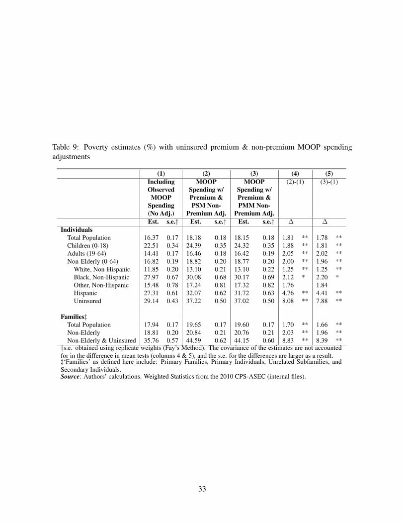
Table 9: Poverty estimates (%) with uninsured premium & non-premium MOOP spendingadjustments
(1) (2) (3) (4) (5)Including MOOP MOOP (2)-(1) (3)-(1)Observed Spending w/ Spending w/MOOP Premium & Premium &
Spending PSM Non- PMM Non-(No Adj.) Premium Adj. Premium Adj.Est. s.e.† Est. s.e.† Est. s.e.† ∆ ∆
IndividualsTotal Population 16.37 0.17 18.18 0.18 18.15 0.18 1.81 ** 1.78 **Children (0-18) 22.51 0.34 24.39 0.35 24.32 0.35 1.88 ** 1.81 **Adults (19-64) 14.41 0.17 16.46 0.18 16.42 0.19 2.05 ** 2.02 **Non-Elderly (0-64) 16.82 0.19 18.82 0.20 18.77 0.20 2.00 ** 1.96 **
White, Non-Hispanic 11.85 0.20 13.10 0.21 13.10 0.22 1.25 ** 1.25 **Black, Non-Hispanic 27.97 0.67 30.08 0.68 30.17 0.69 2.12 * 2.20 *Other, Non-Hispanic 15.48 0.78 17.24 0.81 17.32 0.82 1.76 1.84Hispanic 27.31 0.61 32.07 0.62 31.72 0.63 4.76 ** 4.41 **Uninsured 29.14 0.43 37.22 0.50 37.02 0.50 8.08 ** 7.88 **
Families‡Total Population 17.94 0.17 19.65 0.17 19.60 0.17 1.70 ** 1.66 **Non-Elderly 18.81 0.20 20.84 0.21 20.76 0.21 2.03 ** 1.96 **Non-Elderly & Uninsured 35.76 0.57 44.59 0.62 44.15 0.60 8.83 ** 8.39 **
†s.e. obtained using replicate weights (Fay’s Method). The covariance of the estimates are not accountedfor in the difference in mean tests (columns 4 & 5), and the s.e. for the differences are larger as a result.‡‘Families’ as defined here include: Primary Families, Primary Individuals, Unrelated Subfamilies, andSecondary Individuals.Source: Authors’ calculations. Weighted Statistics from the 2010 CPS-ASEC (internal files).
33

Appendix A
The following tables report model estimates used for the uninsured MOOP spending adjust-ments. Tables A.1 and A.2 present the logit model estimations used to derive the propensityscore of being insured for non-elderly adults (19-64) and children (0-18), respectively (dis-cussed in section 4.2.1). Tables A.3 and A.4 present the GLM Log Link non-premium MOOPspending models, conditional on having health insurance, used for the Predictive Mean Matchfor non-elderly adults (19-64) and children (0-18), respectively (discussed in section 4.2.2).And finally, Tables A.5 and A.6 present WLS models for non-group health insurance premiumspending used for the uninsured premium adjustment/imputations for family and non-familypolicies, respectively (discussed in section 4.3). Regression results in the latter two tables donot take into account the complex survey design of the CPS ASEC (i.e., replicate weights),namely because the models are only used for imputation purposes.
34

Table A.1: Logit model for propensity score of having health insurance, adults 19-64
Coefficient s.e.†
Natural Log of Family Income 0.200 0.007 **Number of Family Members (per age group)
age≤18 0.066 0.011 **18≤age≤64 -0.195 0.016 **age≥64 -0.363 0.034 **
Marital Status (Married=1) 0.823 0.028 **Education (reference = less than H.S. Equivalent)
H.S. Equivalent/Associate’s Degree 0.485 0.033 **Bachelor’s Degree 1.073 0.042 **Master’s/Professional Degree/Ph.D. 1.399 0.064 **
Health Status (reference = Excellent)Very Good -0.175 0.029 **Good -0.383 0.031 **Fair -0.236 0.041 **Poor -0.088 0.073
Disability 0.877 0.051 **Age (reference = 19-24)
25-29 -0.086 0.042 *30-34 -0.032 0.04835-39 0.126 0.047 **40-44 0.267 0.048 **45-49 0.392 0.047 **50-54 0.543 0.049 **55-59 0.614 0.054 **60-64 0.847 0.057 **
Male -0.195 0.018 **Race & Ethnicity (reference = White, Non-Hispanic)
Black, Non-Hispanic family member -0.220 0.033 **Hispanic family member -0.928 0.032 **Other, Non-Hispanic family member -0.385 0.054 **
Residence (reference = South)Northeast 0.579 0.037 **Midwest 0.378 0.033 **West 0.324 0.033 **
Employment Status (reference = unemployed)Employed (Excluding self-employed) 0.282 0.081 **Self-employed -0.172 0.046 **Not in labor force 0.564 0.037 **Full Time Student 1.580 0.060 **
Employer Number of Employees (reference = 0)<25 workers -0.177 0.082 *25-99 workers 0.454 0.088 **100-499 workers 0.770 0.083 **500+ workers 1.067 0.082 **
Industry: Wholesale & Retail Trade -0.106 0.031 **Intercept -2.107 0.091 **
N 123,097
** p<0.01, * p<0.05, + p<0.1†s.e. obtained using replicate weights (Fay’s Method)Notes: Logit model is estimated only on insured non-elderly adults aged 19-64.Dependent variable identifies that the individual has health insurance (any type).Source: Authors’ calculations using the 2010 CPS-ASEC (internal files).
35
Table A.2: Logit model for propensity score of having health insurance, ages 0-18
Coefficient s.e.†
Natural Log of Family Income 0.124 0.009 **Number of Family Members (per age group)
age=18 0.027 0.03018≤age≤64 -0.258 0.028 **age≥64 -0.543 0.059 **
Max Education Family Members (reference = less than H.S. Equivalent)H.S. Equivalent/Associate’s Degree 0.244 0.074 **Bachelor’s Degree 0.868 0.104 **Master’s/Professional Degree/Ph.D. 1.244 0.115 **
Health Status (reference = Excellent)Very Good 0.013 0.055Good -0.107 0.061 +Fair 0.448 0.154 **Poor 0.161 0.356
Age (reference = 1-4 years old)infant -0.349 0.085 **5-9 -0.197 0.050 **10-13 -0.303 0.057 **14-18 -0.568 0.051 **
Male -0.016 0.030Race & Ethnicity (reference = White, Non-Hispanic)
Black, Non-Hispanic family member -0.205 0.074 **Hispanic family member -0.651 0.061 **Other, Non-Hispanic family member -0.403 0.108 **
Residence (reference = South)Northeast 0.582 0.073 **Midwest 0.430 0.074 **West 0.396 0.059 **
Intercept 1.240 0.125 **
N 63,733
** p<0.01, * p<0.05, + p<0.1†s.e. obtained using replicate weights (Fay’s Method)Notes: Logit model is estimated only on insured children aged 0-18. Dependent variable identifiesthat the individual has health insurance (any type).Source: Authors’ calculations using the 2010 CPS-ASEC (internal files).
36

Table A.3: GLM Log Link non-premium MOOP spending model, insured adults 19-64
Coefficient s.e.†
Natural Log of Family Income 0.152 0.021 **Number of Family Members (per age group)
age≤18 -0.019 0.01618≤age≤64 -0.063 0.018 **age≥64 -0.050 0.045
Marital Status (Married=1) 0.102 0.037 **Education (reference = less than H.S. Equivalent)
H.S. Equivalent/Associate’s Degree 0.234 0.067 **Bachelor’s Degree 0.397 0.070 **Master’s/Professional Degree/Ph.D. 0.491 0.073 **
Health Status (reference = Excellent)Very Good 0.089 0.033 **Good 0.552 0.063 **Fair 0.857 0.057 **Poor 1.023 0.104 **
Disability 0.120 0.056 *Age (reference = 19-24)
25-29 0.110 0.15530-34 0.291 0.148 *35-39 0.259 0.15840-44 0.275 0.156 +45-49 0.293 0.160 +50-54 0.511 0.164 **55-59 0.604 0.166 **60-64 0.627 0.164 **
Male -0.156 0.021 **Race & Ethnicity (reference = White, Non-Hispanic)
Black, Non-Hispanic family member -0.404 0.043 **Hispanic family member -0.434 0.040 **Other, Non-Hispanic family member -0.347 0.074 **
Residence (reference = South)Northeast -0.383 0.041 **Midwest -0.151 0.050 **West -0.032 0.048
Employment Status (reference = unemployed)Employed (Excluding self-employed) 0.228 0.133 +Self-employed 0.280 0.061 **Not in labor force 0.004 0.053Full Time Student -0.018 0.165
Employer Number of Employees (reference = 0)<25 workers -0.174 0.12925-99 workers -0.188 0.128100-499 workers -0.205 0.132500+ workers -0.189 0.125
Industry: Wholesale & Retail Trade 0.015 0.044Intercept 4.318 0.218 **
N
** p<0.01, * p<0.05, + p<0.1†s.e. obtained using replicate weights (Fay’s Method)Notes: GLM log link model is estimated only on insured (any type) non-elderlyadults aged 19-64. Dependent variable equals total non-premium MOOP spend-ing (2009 $).Source: Authors’ calculations using the 2010 CPS-ASEC (internal files).
37

Table A.4: GLM Log Link non-premium MOOP spending model, insured children 0-18
Coefficient s.e.†
Natural Log of Family Income 0.317 0.056 **Number of Family Members (per age group)
age≤18 -0.131 0.020 **18≤age≤64 -0.185 0.031 **age≥64 -0.204 0.070 **
Max Education Family Members (reference = less than H.S. Equivalent)H.S. Equivalent/Associate’s Degree 0.557 0.128 **Bachelor’s Degree 0.869 0.127 **Master’s/Professional Degree/Ph.D. 0.902 0.128 **
Health Status (reference = Excellent)Very Good 0.116 0.041 **Good 0.577 0.074 **Fair 1.599 0.154 **Poor 1.832 0.195 **
Infant (reference = age>1 year old) 0.077 0.081Male 0.004 0.042Race & Ethnicity (reference = White, Non-Hispanic)
Black, Non-Hispanic family member -0.557 0.070 **Hispanic family member -0.298 0.087 **Other, Non-Hispanic family member -0.226 0.069 **
Residence (reference = South)Northeast -0.189 0.069 **Midwest -0.044 0.052West -0.043 0.056
Intercept 2.061 0.650 **
N
** p<0.01, * p<0.05, + p<0.1†s.e. obtained using replicate weights (Fay’s Method)Notes: GLM log link model is estimated only on insured children aged 0-18. Dependent variableequals total non-premium MOOP spending (2009 $). Model is limited only to insured individuals(any type).Source: Authors’ calculations using the 2010 CPS-ASEC (internal files).
38

Table A.5: Non-group premium expenditure model (WLS), family policies
Coefficient s.e.
Number of Individuals on Policy (per age group)0-18 686.8 143.5 **19-34 357.1 238.035-39 1,162.9 350.6 **40-44 1,169.3 321.7 **45-49 2,207.2 303.4 **50-54 2,099.9 314.8 **55-59 1,854.6 341.1 **60-64 3,672.7 373.2 **
Married 1,157.4 427.2 **Number of Individuals on Policy Reporting Fair/Poor Health 2,111.0 969.0 *Intercept 1,062.5 522.6 *
N 1,005
Adjusted R-Squared 0.16
** p<0.01, * p<0.05, + p<0.1Notes: WLS model is estimated only for policyholders of family non-group health insurancepolicies. Dependent variable is total premium spending (2009 $).Source: Authors’ calculations using the 2010 CPS-ASEC (internal files).
Table A.6: Non-group premium expenditure model (WLS), single person policies
Coefficient s.e.
Age of Policyholder (reference = age 15-18)19-34 407.4 1,470.635-39 1,217.0 1,493.540-44 2,504.9 1,485.8 +45-49 2,206.0 1,481.350-54 2,810.6 1,478.2 +55-59 2,932.2 1,477.8 *60-64 4,110.3 1,475.9 **
Intercept 1,262.1 1,466.0
N 1,564
Adjusted R-Squared 0.20
** p<0.01, * p<0.05, + p<0.1Notes: WLS model is estimated only for policyholders of single (non-family) non-group health insurance policies. Dependent variable is totalpremium spending (2009 $).Source: Authors’ calculations using the 2010 CPS-ASEC (internal files).
39