Medical Statistics Medical Statistics (full English class)(full English class)

Ji-Qian Fang

School of Public Health

Sun Yat-Sen University

Chapter 10

Statistical Analysis of Enumeration Data

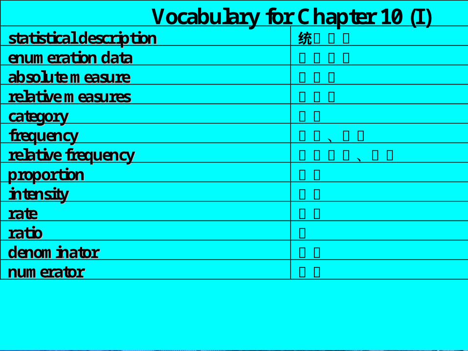
Vocabulary for Chapter 10 (I) ssttaattiissttiiccaall ddeessccrriippttiioonn 统计描述

eennuummeerraattiioonn ddaattaa 计数资料

aabbssoolluuttee mmeeaassuurree 绝对量

rreellaattiivvee mmeeaassuurreess 相对量

ccaatteeggoorryy 类别

ffrreeqquueennccyy 频数、频率

rreellaattiivvee ffrreeqquueennccyy 相对频数、频率

pprrooppoorrttiioonn 比率

iinntteennssiittyy 强度

rraattee 速率

rraattiioo 比

ddeennoommiinnaattoorr 分母

nnuummeerraattoorr 分子

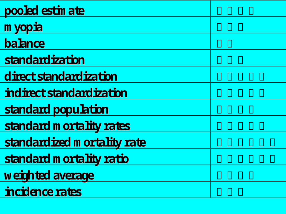
ppoooolleedd eessttiimmaattee 联合估计

mmyyooppiiaa 近视眼

bbaallaannccee 均衡

ssttaannddaarrddiizzaattiioonn 标准化

ddiirreecctt ssttaannddaarrddiizzaattiioonn 直接标准化

iinnddiirreecctt ssttaannddaarrddiizzaattiioonn 间接标准化

ssttaannddaarrdd ppooppuullaattiioonn 标准人口

ssttaannddaarrdd mmoorrttaalliittyy rraatteess 标准死亡率

ssttaannddaarrddiizzeedd mmoorrttaalliittyy rraattee 标准化死亡率

ssttaannddaarrdd mmoorrttaalliittyy rraattiioo 标准死亡率比

wweeiigghhtteedd aavveerraaggee 加权平均

iinncciiddeennccee rraatteess 发病率

10.1 Statistical Description 10.1 Statistical Description forfor

enumeration data enumeration data

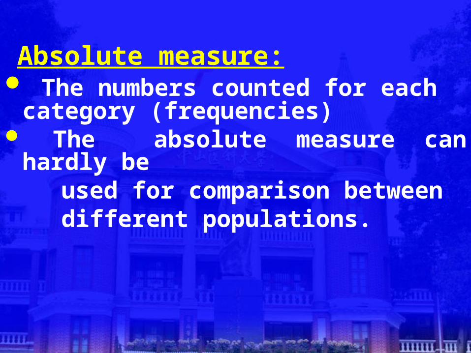
Absolute measure: The numbers counted for each

category (frequencies) The absolute measure can

hardly be used for comparison between different populations.

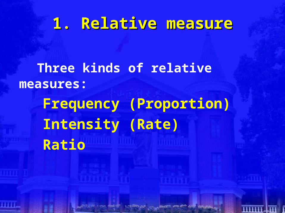
1. Relative measure1. Relative measure Three kinds of relative measures:

Frequency (Proportion) Intensity (Rate) Ratio

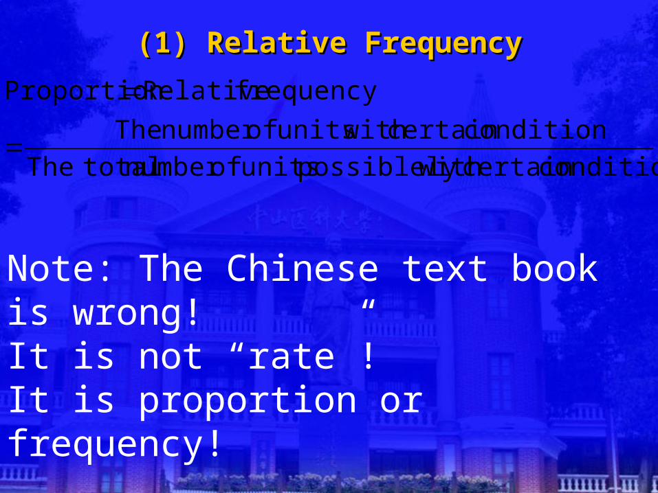
(1) Relative Frequency(1) Relative Frequency

condition certain with possiblely units ofnumber totalThe

conditioncertain with units ofnumber The

frequency Relative Proportion

Note: The Chinese text book is wrong!It is not “rate”!It is proportion or frequency!

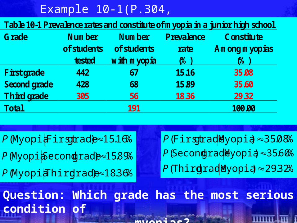
Example 10-1(P.304, revised)

%16.15)gradeFirst Myopia( P

%89.15)grade SecondMyopia( P

%36.18)grade ThirdMyopia( P

%08.35)MyopiagradeFirst ( P%60.35)Myopiagrade Second( P

%32.29)Myopiagrade Third( P

Question: Which grade has the most serious condition of myopias?

Table 10-1 Prevalence rates and constitute of myopia in a junior high school Grade Number

of students tested

Number of students

with myopia

Prevalence rate (%)

Constitute Among myopias

(%) First grade 442 67 15.16 35.08 Second grade 428 68 15.89 35.60 Third grade 305 56 18.36 29.32 Total 191 100.00

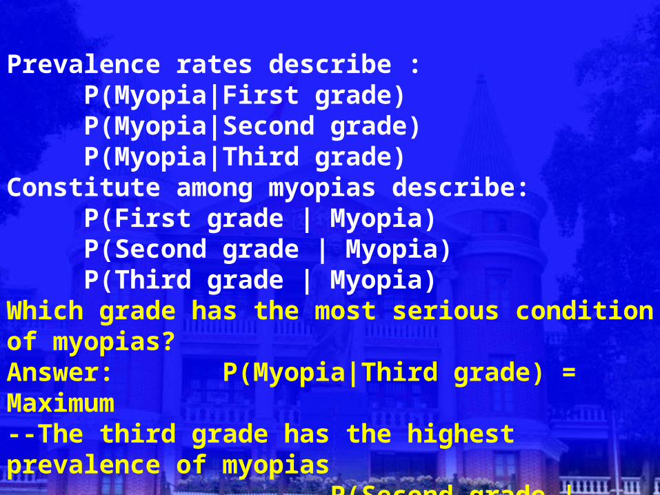
Prevalence rates describe : P(Myopia|First grade) P(Myopia|Second grade) P(Myopia|Third grade)Constitute among myopias describe: P(First grade | Myopia) P(Second grade | Myopia) P(Third grade | Myopia)Which grade has the most serious condition of myopias?Answer: P(Myopia|Third grade) = Maximum --The third grade has the highest prevalence of myopias P(Second grade | Myopia)= Maximum -- Among the myopias, the absolute number of Second grade students is the highest.

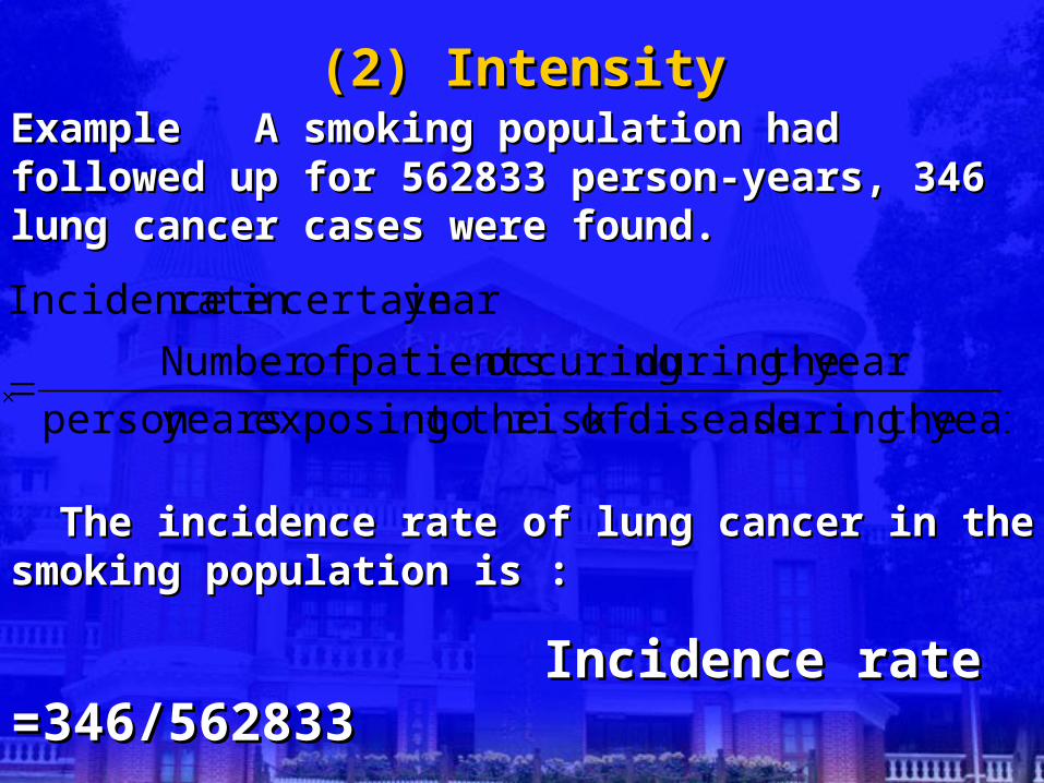
(2) Intensity(2) IntensityExample A smoking population had Example A smoking population had followed up for 562833 person-years, 346 followed up for 562833 person-years, 346 lung cancer cases were found.lung cancer cases were found.

The incidence rate of lung cancer in the The incidence rate of lung cancer in the smoking population is :smoking population is :

Incidence rate =346/562833Incidence rate =346/562833

=61.47 per 100,000 person-year=61.47 per 100,000 person-year

year theduring disease ofrisk the toexposing yearsperson

year theduring occuring patients ofNumber

yearcertain in rate Incidence

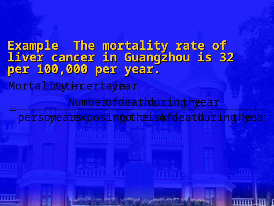
year theduringdeath ofrisk the toexposing yearsperson

year theduring deaths ofNumber

yearcertain in rateMortality

Example The mortality rate of liver cancer in Example The mortality rate of liver cancer in Guangzhou is 32 per 100,000 per year.Guangzhou is 32 per 100,000 per year.

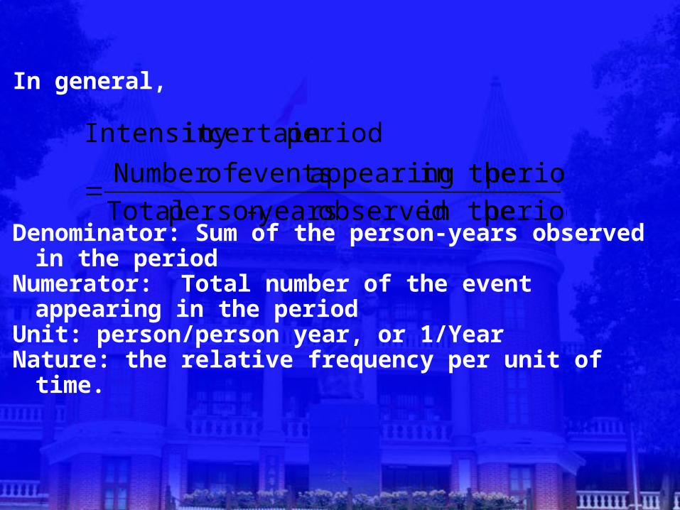
period in the observed years-person Total

period in the appearing events ofNumber

periodcertain in Intensity

In general,

Denominator: Sum of the person-years observed in the period

Numerator: Total number of the event appearing in the period

Unit: person/person year, or 1/YearNature: the relative frequency per unit of time.

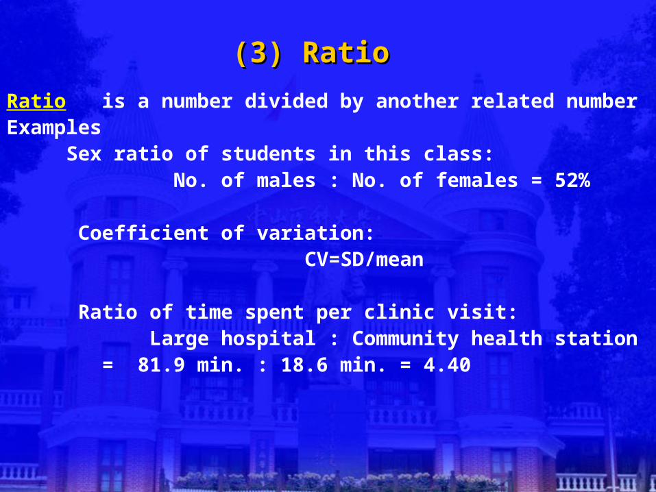
(3) Ratio(3) Ratio Ratio is a number divided by another related numberExamples Sex ratio of students in this class: No. of males : No. of females = 52%

Coefficient of variation: CV=SD/mean Ratio of time spent per clinic visit: Large hospital : Community health station = 81.9 min. : 18.6 min. = 4.40

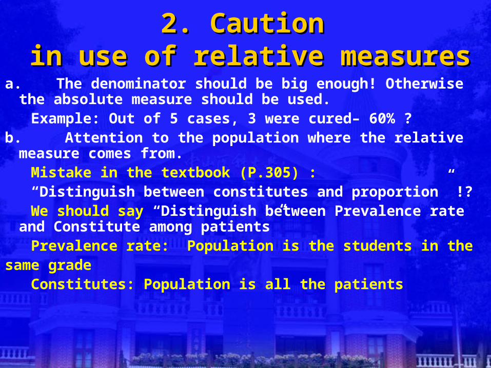
2. Caution 2. Caution in use of relative measuresin use of relative measures

a. The denominator should be big enough! Otherwise the absolute measure should be used.

Example: Out of 5 cases, 3 were cured– 60% ?b. Attention to the population where the relative

measure comes from. Mistake in the textbook (P.305) : “Distinguish between constitutes and proportion” !? We should say “Distinguish between Prevalence

rate and Constitute among patients” Prevalence rate: Population is the students in thesame grade Constitutes: Population is all the patients

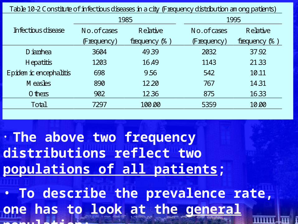
Table 10-2 Constitute of infectious diseases in a city (Frequency distribution among patients)

1985 1995

Infectious disease No. of cases

(Frequency)

Relative

frequency (%)

No. of cases

(Frequency)

Relative

frequency (%)

Diarrhea 3604 49.39 2032 37.92

Hepatitis 1203 16.49 1143 21.33

Epidemic encephalitis 698 9.56 542 10.11

Measles 890 12.20 767 14.31

Others 902 12.36 875 16.33

Total 7297 100.00 5359 10.00

• The above two frequency distributions reflect two populations of all patients;

• To describe the prevalence rate, one has to look at the general population;

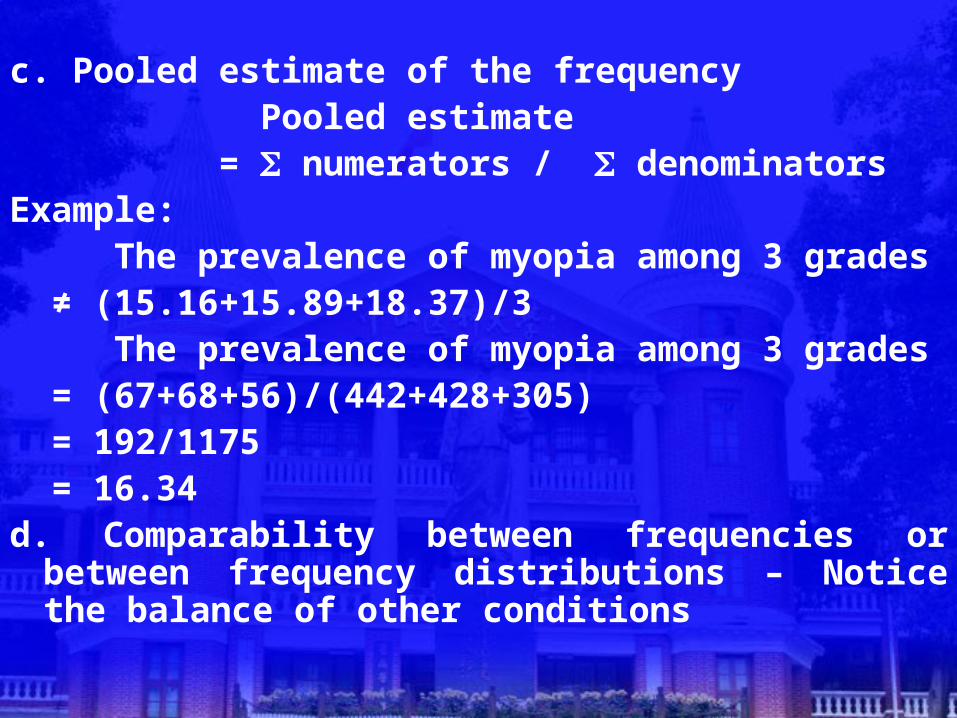
c. Pooled estimate of the frequency Pooled estimate = numerators / denominators Example: The prevalence of myopia among 3 grades ≠ (15.16+15.89+18.37)/3 The prevalence of myopia among 3 grades = (67+68+56)/(442+428+305) = 192/1175 = 16.34d. Comparability between frequencies or

between frequency distributions – Notice the balance of other conditions

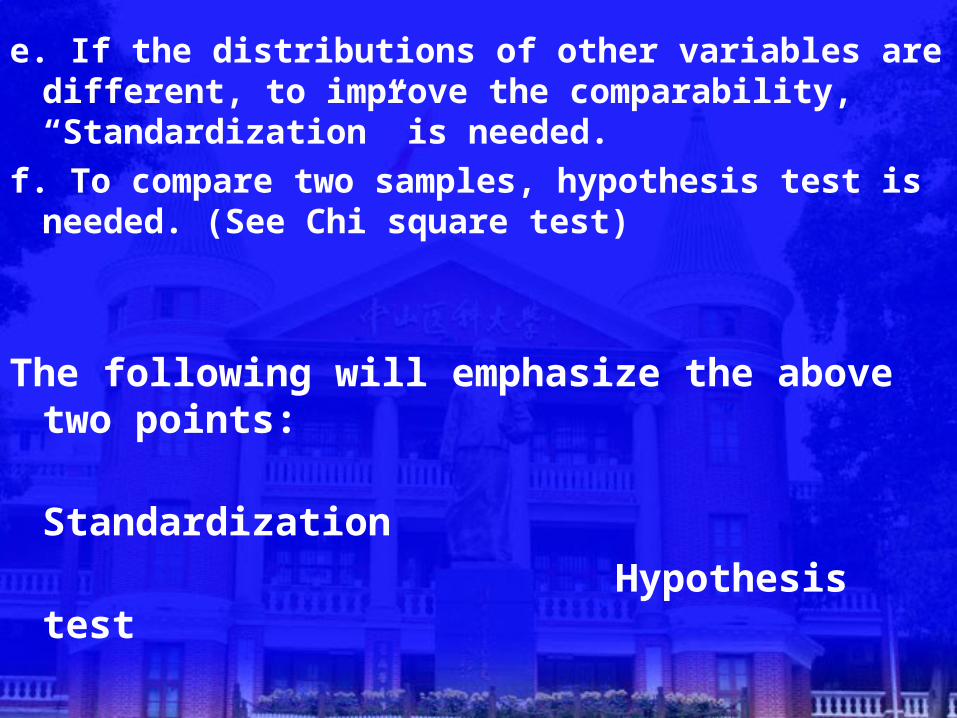
e. If the distributions of other variables are different, to improve the comparability, “Standardization” is needed.

f. To compare two samples, hypothesis test is needed. (See Chi square test)

The following will emphasize the above two points:

Standardization

Hypothesis test

3. Standardization for 3. Standardization for crude frequency or crude intensitycrude frequency or crude intensity

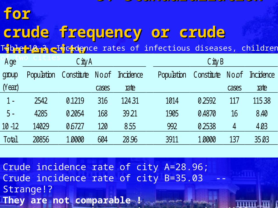
Crude incidence rate of city A=28.96; Crude incidence rate of city B=35.03 -- Strange!?

They are not comparable ! -- Because the constitute are quite different

City A City B Age

group

(Year)

Population Constitute No.of

cases

Incidence

rate

Population Constitute No.of

cases

Incidence

rate

1 - 2542 0.1219 316 124.31 1014 0.2592 117 115.38

5 - 4285 0.2054 168 39.21 1905 0.4870 16 8.40

10 -12 14029 0.6727 120 8.55 992 0.2538 4 4.03

Total 20856 1.0000 604 28.96 3911 1.0000 137 35.03

Table 10-3 Incidence rates of infectious diseases, children of two cities

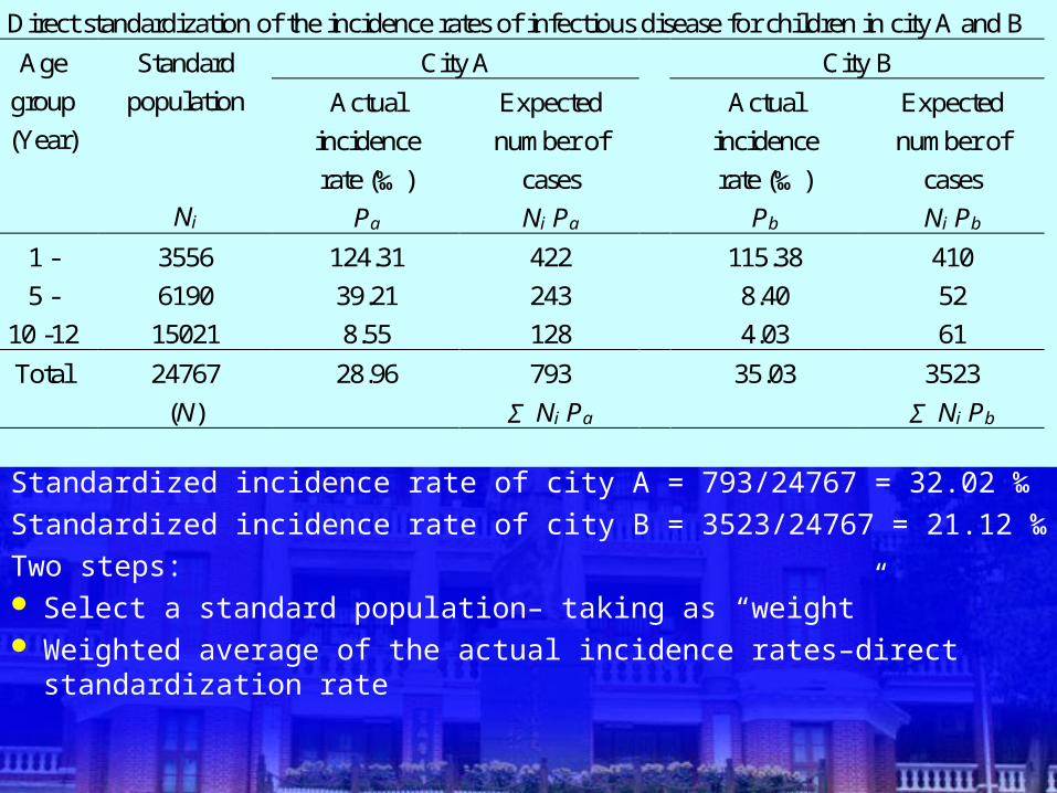
Standardized incidence rate of city A = 793/24767 = 32.02 ‰

Standardized incidence rate of city B = 3523/24767 = 21.12 ‰

Two steps: Select a standard population– taking as “weight” Weighted average of the actual incidence rates–direct standardization rate

Direct standardization of the incidence rates of infectious disease for children in city A and B

City A City B Age

group

(Year)

Standard

population

Ni

Actual

incidence

rate (‰)

Pa

Expected

number of

cases

Ni Pa

Actual

incidence

rate (‰)

Pb

Expected

number of

cases

Ni Pb

1 - 3556 124.31 422 115.38 410

5 - 6190 39.21 243 8.40 52

10 -12 15021 8.55 128 4.03 61

Total 24767

(N)

28.96 793

Σ Ni Pa

35.03 3523

Σ Ni Pb

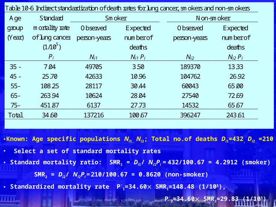
•Known: Age specific populations Ni1, Ni2; Total no.of deaths Di1=432, Di2 =210

• Select a set of standard mortality rates

• Standard mortality ratio: SMR1 = Di1/ Ni1Pi = 432/100.67 = 4.2912 (smoker)

SMR2 = Di2/ Ni2Pi = 210/100.67 = 0.8620 (non-smoker)

• Standardized mortality rate P’1=34.60 SMR1=148.48 (1/105),

P’2=34.60 SMR2=29.83 (1/105)

Table 10-6 Indirect standardization of death rates for lung cancer, smokers and non-smokers

Smoker Non-smoker Age

group

(Year)

Standard

mortality rate

of lung cancer

(1/105)

Pi

Observed

person-years

Ni1

Expected

number of

deaths

Ni1 Pi

Observed

person-years

Ni2

Expected

number of

deaths

Ni2 Pi

35 - 7.04 49705 3.50 189370 13.33

45 - 25.70 42633 10.96 104762 26.92

55- 108.25 28117 30.44 60043 65.00

65- 263.94 10624 28.04 27540 72.69

75- 451.87 6137 27.73 14532 65.67

Total 34.60 137216 100.67 396247 243.61

10.2 Statistical Inference

for

Enumeration Data

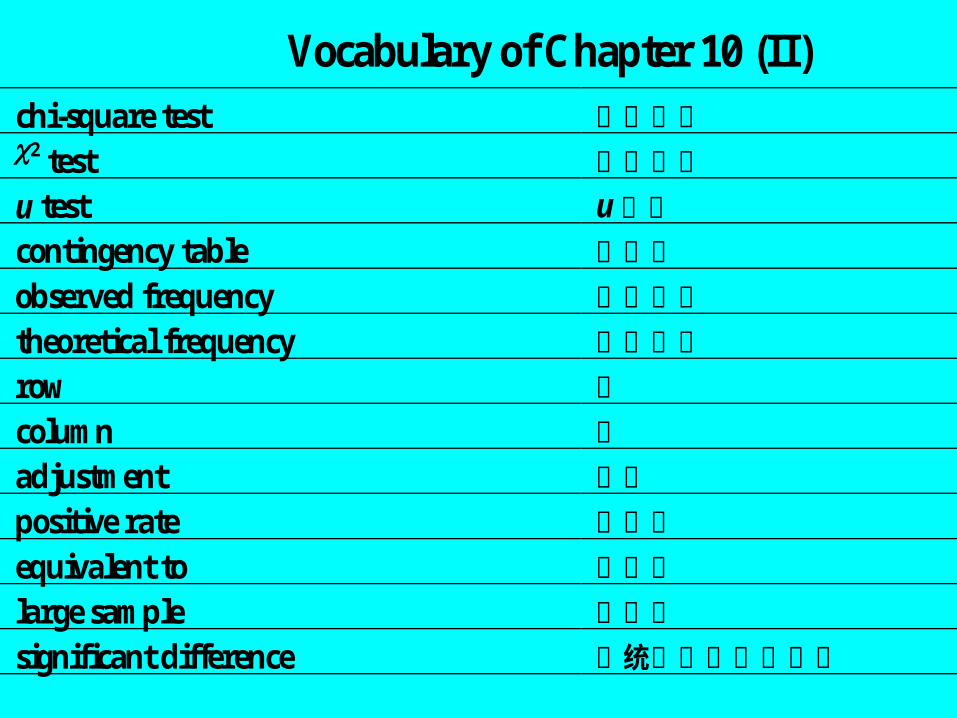
Vocabulary of Chapter 10 (II)

chi-square test 卡方检验 2 test 卡方检验

u test u检验

contingency table 列联表

observed frequency 观察频数

theoretical frequency 理论频数

row 行

column 列

adjustment 校正

positive rate 阳性率

equivalent to 等价于

large sample 大样本

significant difference 有统计学意义的差异

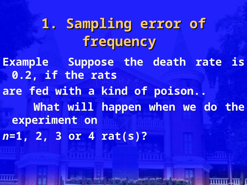
1. Sampling error of frequency1. Sampling error of frequency

Example Suppose the death rate is 0.2, if the rats

are fed with a kind of poison..

What will happen when we do the experiment on

n=1, 2, 3 or 4 rat(s)?

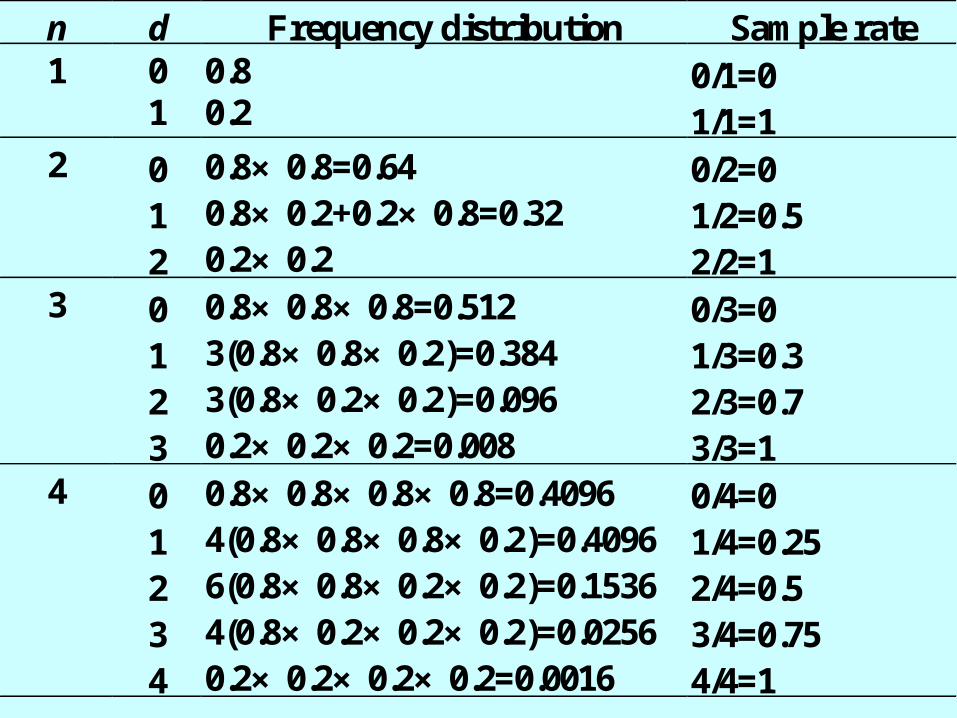
n d Frequency distribution Sample rate 1 0

1 0.8 0.2

0/1=0 1/1=1

2 0 1 2

0.8× 0.8=0.64 0.8× 0.2+0.2× 0.8=0.32 0.2× 0.2

0/2=0 1/2=0.5 2/2=1

3 0 1 2 3

0.8× 0.8× 0.8=0.512 3(0.8× 0.8× 0.2)=0.384 3(0.8× 0.2× 0.2)=0.096 0.2× 0.2× 0.2=0.008

0/3=0 1/3=0.3 2/3=0.7 3/3=1

4 0 1 2 3 4

0.8× 0.8× 0.8× 0.8=0.4096 4(0.8× 0.8× 0.8× 0.2)=0.4096 6(0.8× 0.8× 0.2× 0.2)=0.1536 4(0.8× 0.2× 0.2× 0.2)=0.0256 0.2× 0.2× 0.2× 0.2=0.0016

0/4=0 1/4=0.25 2/4=0.5 3/4=0.75 4/4=1

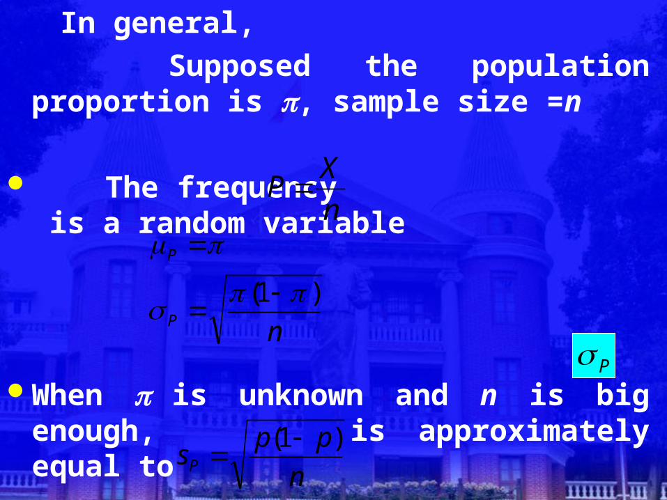
In general,

Supposed the population proportion is , sample size =n

The frequency is a random variable

When is unknown and n is big enough, is approximately equal to

nP

P

)1(

n

XP

n

ppsP

)1(

P

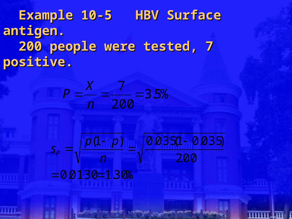
Example 10-5 HBV Surface antigen. Example 10-5 HBV Surface antigen. 200 people were tested, 7 positive. 200 people were tested, 7 positive.

%5.3200

7

n

XP

%30.10130.0200

)035.01(035.0)1(

n

ppsP

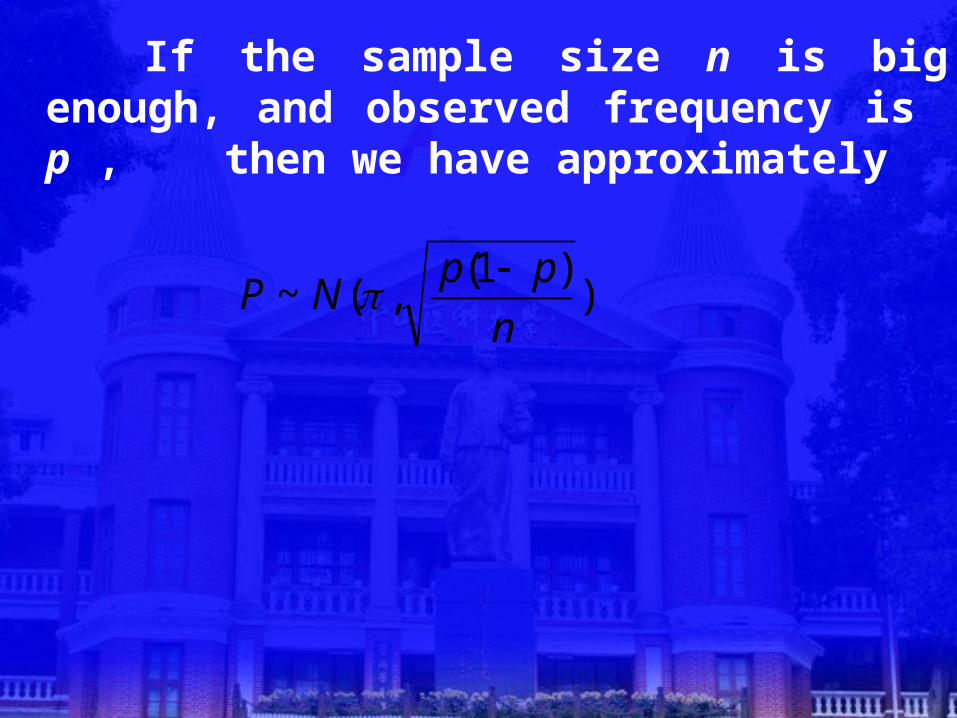
If the sample size n is big enough, and observed frequency is p , then we have approximately

))1(

,(~n

ppNP

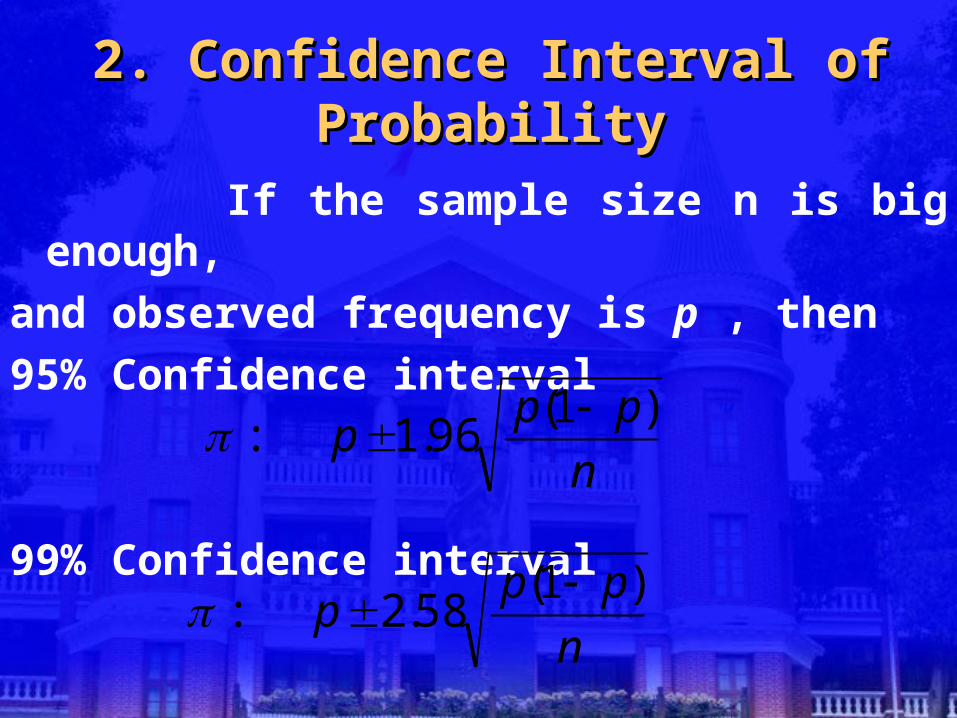
2. Confidence Interval of Probability2. Confidence Interval of Probability

If the sample size n is big enough,

and observed frequency is p , then

95% Confidence interval

99% Confidence intervaln

ppp

)1(96.1:

n

ppp

)1(58.2:

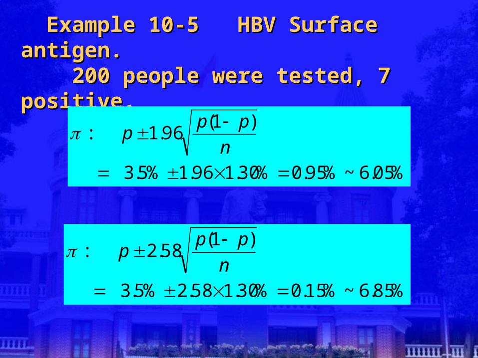
Example 10-5 HBV Surface antigen. Example 10-5 HBV Surface antigen. 200 people were tested, 7 positive. 200 people were tested, 7 positive.

%05.6~%95.0%30.196.1%5.3

)1(96.1:

n

ppp

%85.6~%15.0%30.158.2%5.3

)1(58.2:

n

ppp

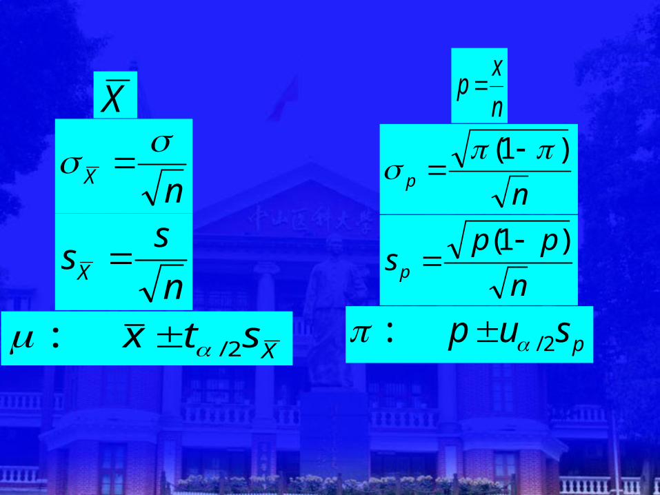
X n

xp

nX

n

p

)1(

n

ssX

n

ppsp

)1(

Xstx 2/: psup 2/:

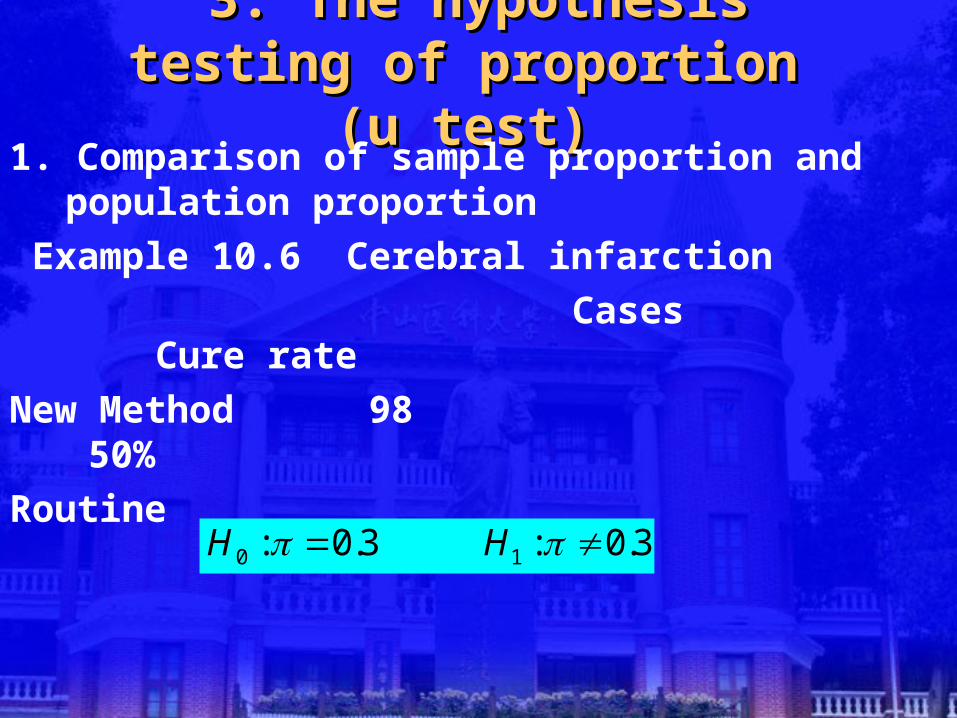
3. The hypothesis testing of 3. The hypothesis testing of proportion (u test)proportion (u test)

1. Comparison of sample proportion and population proportion

Example 10.6 Cerebral infarction

Cases Cure rate

New Method 98 50%

Routine 30%

3.0:3.0: 10 HH

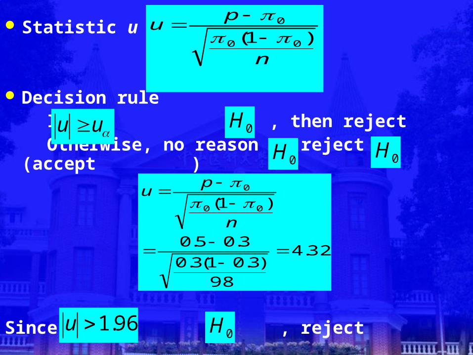
Statistic u

Decision rule If , then reject Otherwise, no reason to reject (accept )

Since , reject

uu 0H

0H

96.1u0H

n

pu

)1( 00

0

32.4

98)3.01(3.0

3.05.0

)1( 00

0

n

pu

0H

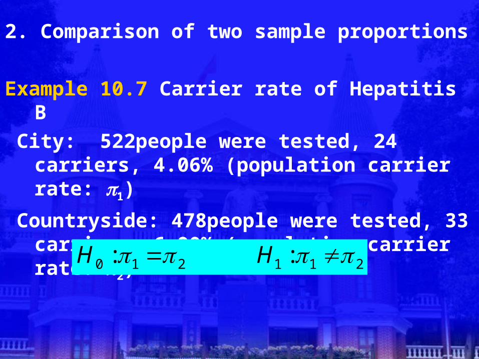
2. Comparison of two sample proportions

Example 10.7 Carrier rate of Hepatitis B

City: 522people were tested, 24 carriers, 4.06% (population carrier rate: 1)

Countryside: 478people were tested, 33 carriers, 6.90% (population carrier rate: 2)

211210 :: HH

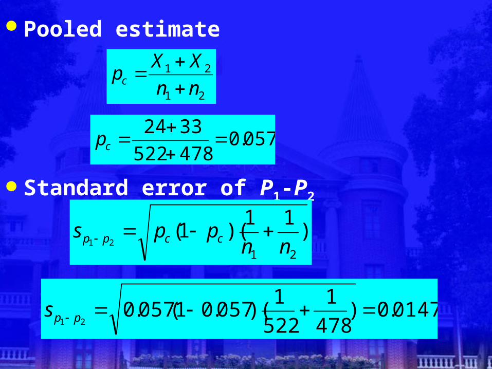
Pooled estimate

Standard error of P1-P2

21

21

nn

XXpc

057.0478522

3324

cp

)11

)(1(21

21 nnpps ccpp

0147.0)478

1

522

1)(057.01(057.0

21 pps

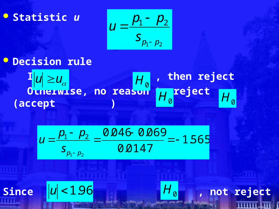
Statistic u

Decision rule

If , then reject

Otherwise, no reason to reject (accept )

Since , not reject

21

21

pps

ppu

uu 0H

0H

565.10147.0

069.0046.0

21

21

pps

ppu

96.1u 0H

0H

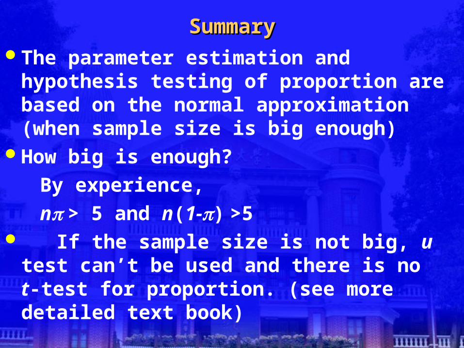
SummarySummaryThe parameter estimation and hypothesis

testing of proportion are based on the normal approximation (when sample size is big enough)

How big is enough?

By experience,

n > 5 and n(1-) >5 If the sample size is not big, u test can’t be

used and there is no t-test for proportion. (see more detailed text book)

10.3 Chi-square test10.3 Chi-square test

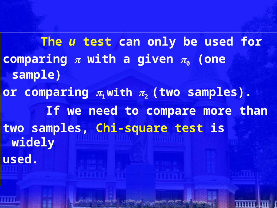
The u test can only be used for comparing with a given 0 (one

sample)or comparing 1 with 2 (two samples).

If we need to compare more thantwo samples, Chi-square test is widelyused.

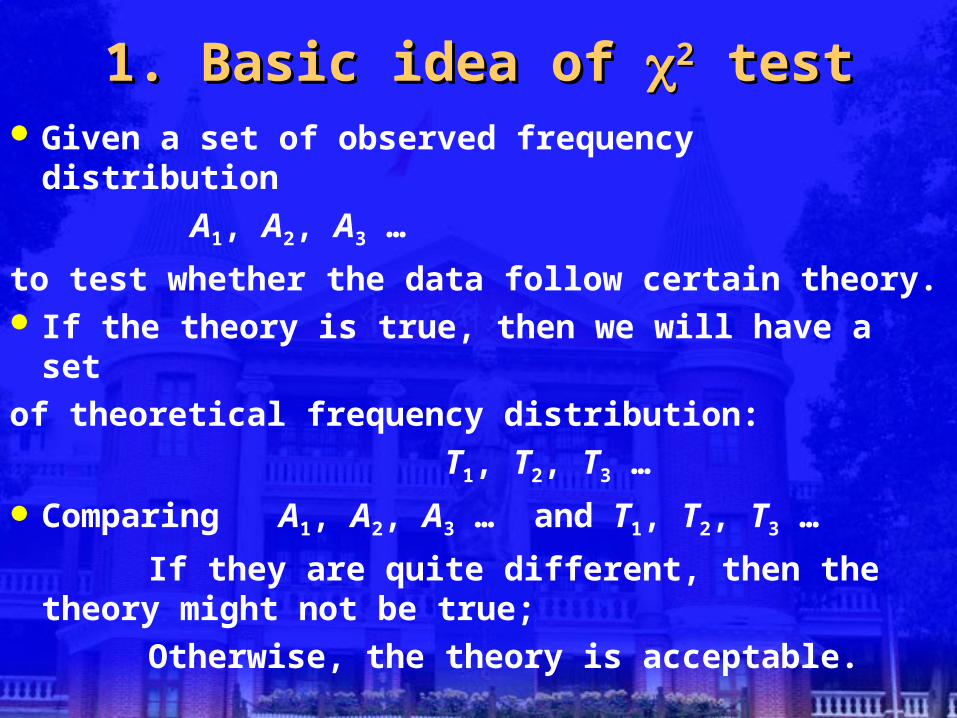
1. Basic idea of 1. Basic idea of 22 test test Given a set of observed frequency distribution A1, A2, A3 …

to test whether the data follow certain theory. If the theory is true, then we will have a set of theoretical frequency distribution: T1, T2, T3 …

Comparing A1, A2, A3 … and T1, T2, T3 …

If they are quite different, then the theory might not be true;

Otherwise, the theory is acceptable.

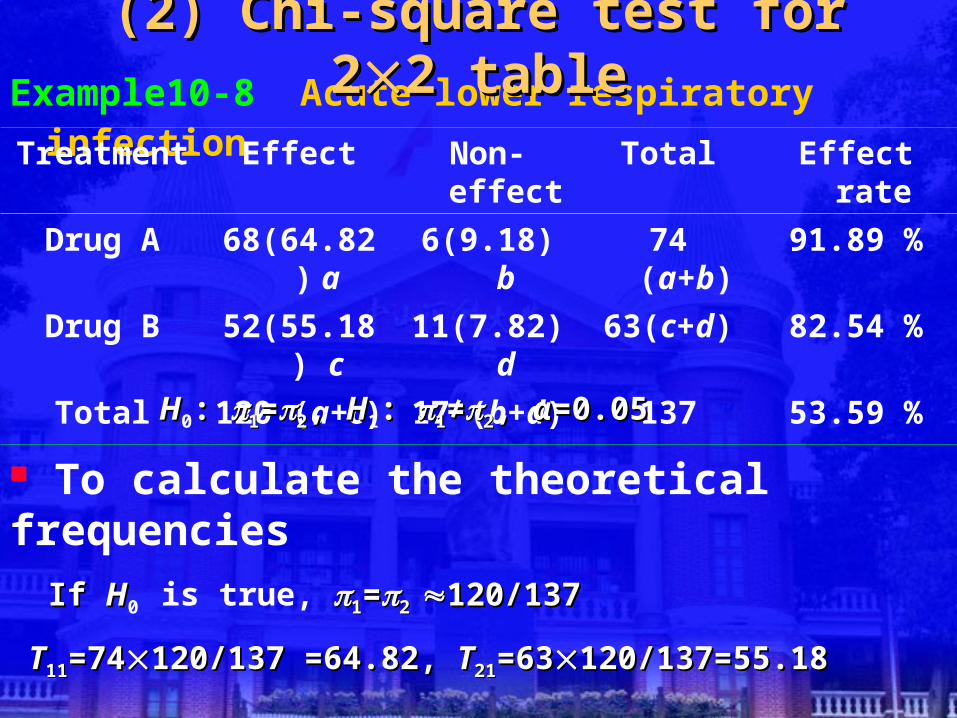
Example10-8 Acute lower respiratory infection Treatment Effect Non-effect Total Effect rate

Drug A 68(64.82) a 6(9.18) b 74 (a+b) 91.89 %

Drug B 52(55.18) c 11(7.82) d 63(c+d) 82.54 %

Total 120 (a+c) 17 (b+d) 137 53.59 %

(2) Chi-square test for 2(2) Chi-square test for 22 table2 table

HH0: : 11==22, , HH1: : 11≠≠22, , αα=0.05 =0.05

To calculate the theoretical frequencies If If HH0 is true, 11==2 2 120/137120/137

TT1111=74=74120/137 =64.82, 120/137 =64.82, TT2121=63=63120/137=55.18120/137=55.18

TT1212=74=7417/137 =9.18, 17/137 =9.18, TT2222=63=6317/137=7.8217/137=7.82

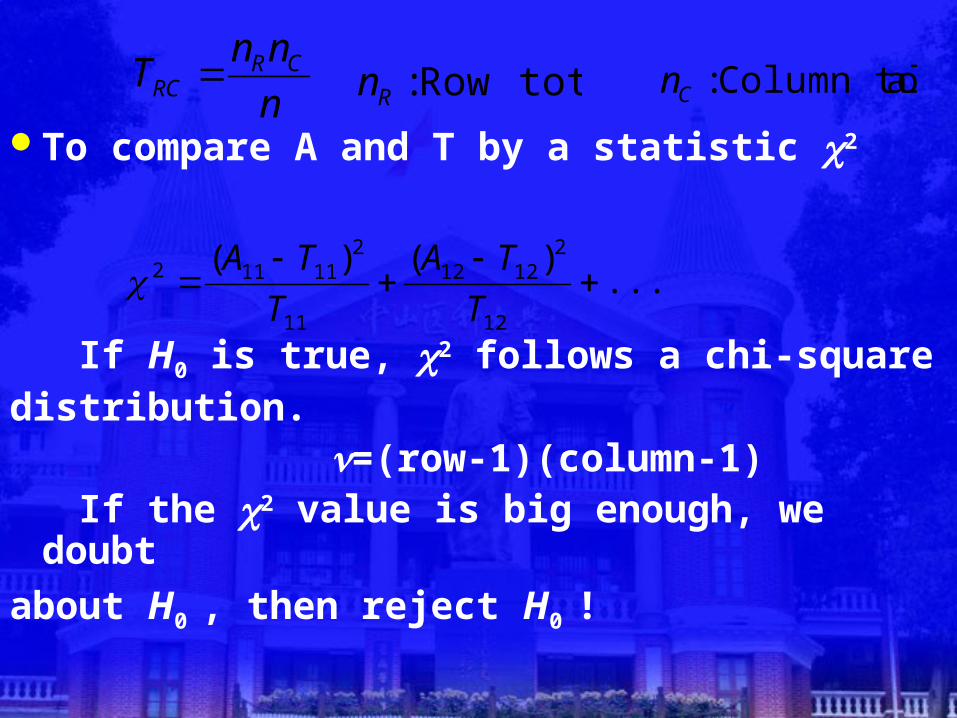
To compare A and T by a statistic 2

If H0 is true, 2 follows a chi-square distribution. =(row-1)(column-1) If the 2 value is big enough, we doubt about H0 , then reject H0 !

......)()(

12

21212

11

211112

T

TA

T

TA

n

nnT CR

RC totalRow :Rn alColumn tot :Cn

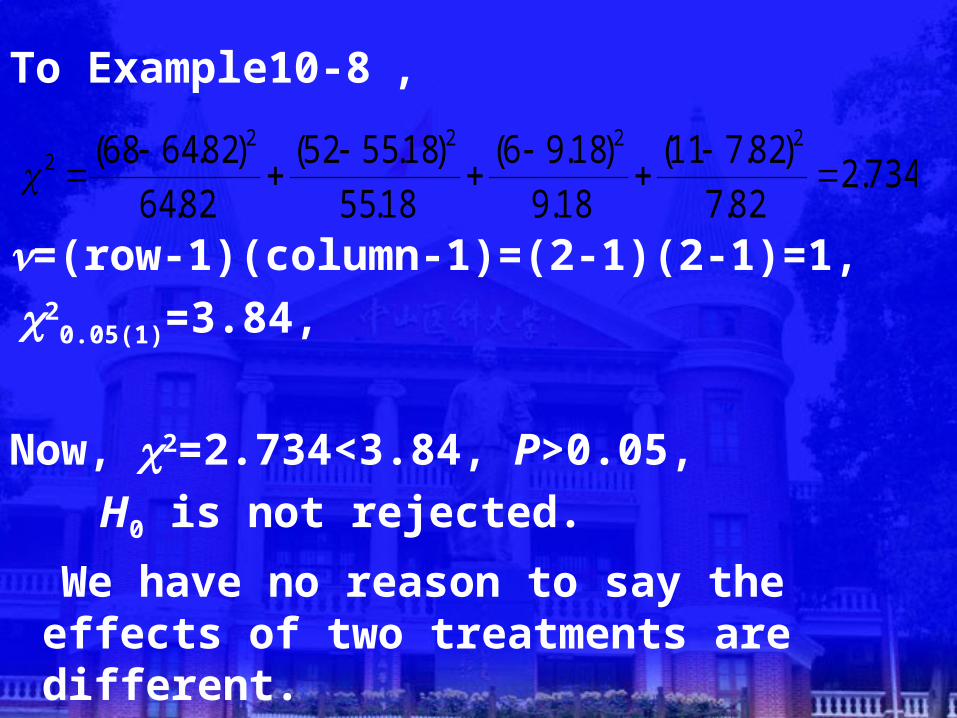
To Example10-8 ,

=(row-1)(column-1)=(2-1)(2-1)=1, 2

0.05(1)=3.84,

Now, 2=2.734<3.84, P>0.05, H0 is not rejected.

We have no reason to say the effects of two treatments are different.

734.282.7

)82.711(

18.9

)18.96(

18.55

)18.5552(

82.64

)82.6468( 22222

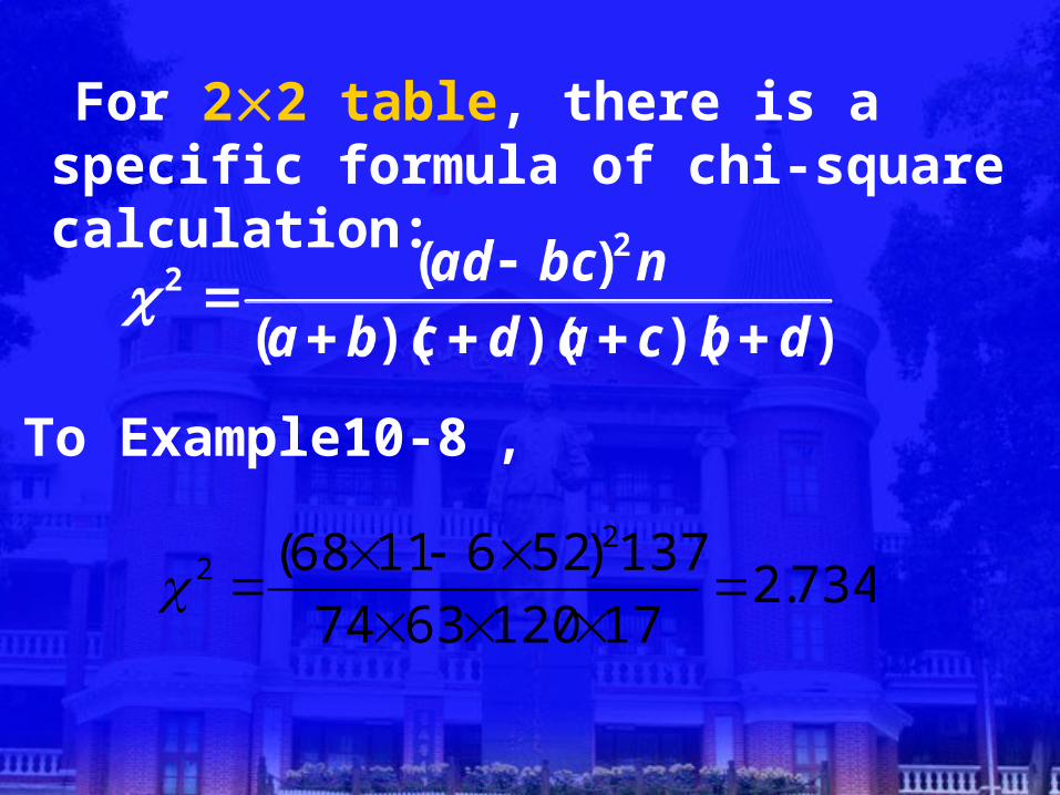
For 22 table, there is a specific formula of chi-square calculation:

734.2171206374

137)5261168( 22

To Example10-8 ,

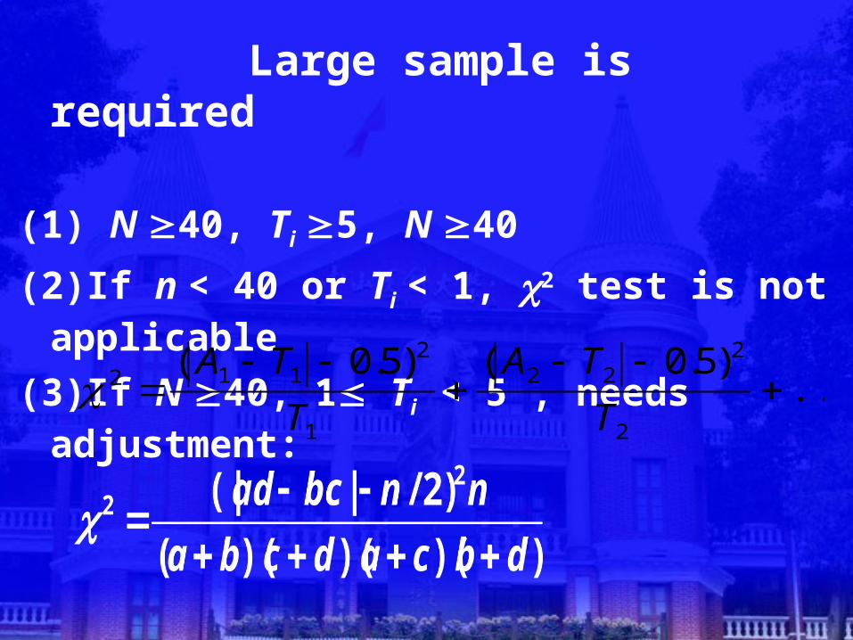
Large sample is required

(1) N 40, Ti 5, N 40

(2)If n < 40 or Ti < 1, 2 test is not applicable

(3)If N 40, 1 Ti < 5 , needs adjustment: ...

)5.0()5.0(

2

222

1

2112

T

TA

T

TA

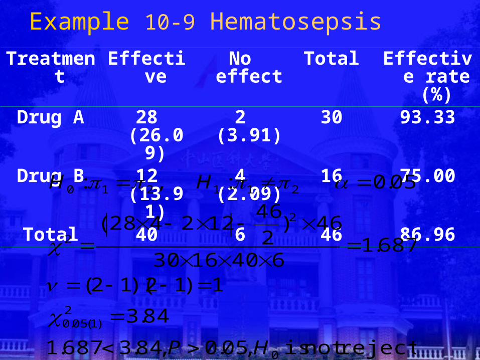
Example 10-9 Hematosepsis

Treatment Effective No effect Total Effective rate (%)

Drug A 28 (26.09) 2 (3.91) 30 93.33

Drug B 12 (13.91) 4 (2.09) 16 75.00

Total 40 6 46 86.96

rejectednot is ,05.0,84.3687.1

84.3

1)12)(12(

687.16401630

46)246

122428(

05.0:,:

0

2)1(05.0

2

2

211210

HP

HH

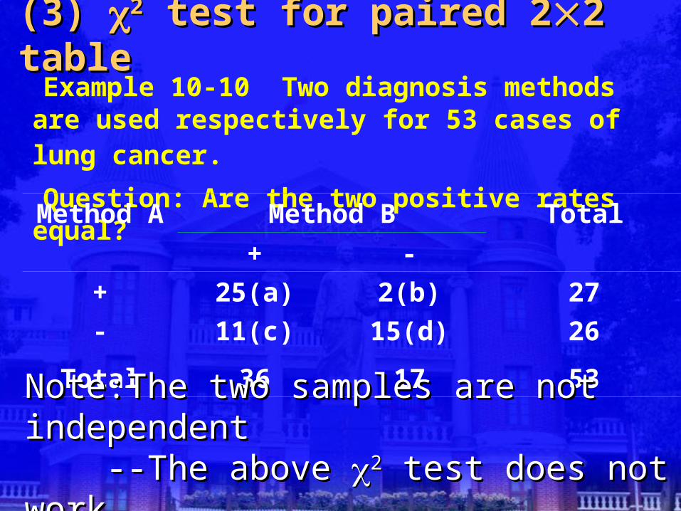
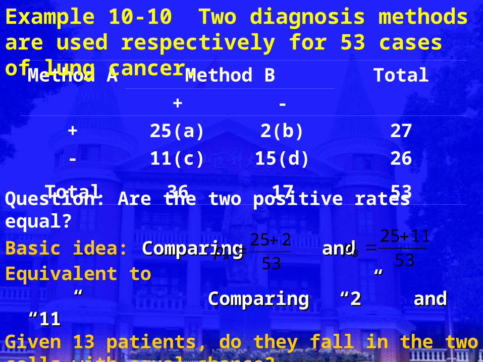
(3) (3) 22 test for paired 2 test for paired 22 table2 table Example 10-10 Two diagnosis methods

are used respectively for 53 cases of lung cancer.

Question: Are the two positive rates equal?

Method A Method B Total

+ -

+ 25(a) 2(b) 27

- 11(c) 15(d) 26

Total 36 17 53

Note:The two samples are not independentNote:The two samples are not independent --The above --The above 22 test does not work test does not work

Method A Method B Total

+ -

+ 25(a) 2(b) 27

- 11(c) 15(d) 26

Total 36 17 53Question: Are the two positive rates equal?Basic idea: ComparingComparing and and Equivalent to ComparingComparing “2” “2” and and “11”“11”Given 13 patients, do they fall in the two cells with equal chance?

Example 10-10 Two diagnosis methods are used respectively for 53 cases of lung cancer.

53

225 Ap

53

1125 Bp

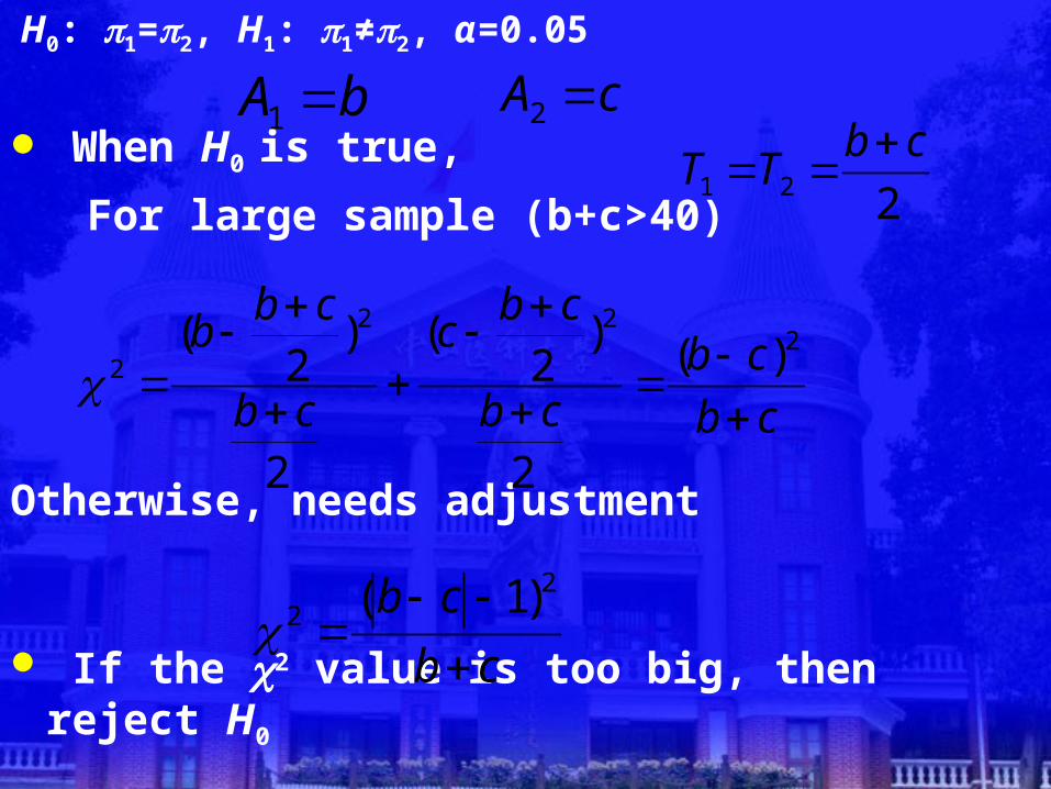
H0: 1=2, H1: 1≠2, α=0.05

When H0 is true,

For large sample (b+c>40)

Otherwise, needs adjustment

If the 2 value is too big, then reject H0

bA 1cA 2

221

cbTT

cb

cbcb

cbc

cb

cbb

222

2 )(

2

)2

(

2

)2

(

cb

cb

2

2 )1(

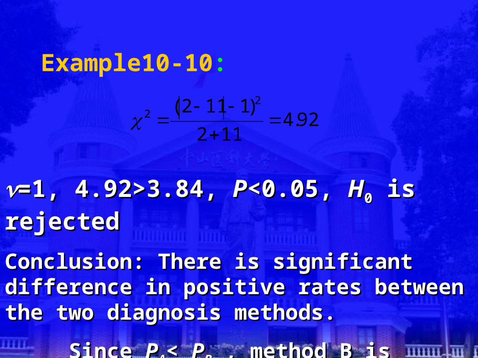
Example10-10:

=1, 4.92>3.84, =1, 4.92>3.84, PP<0.05, <0.05, HH00 is is rejectedrejected

Conclusion: There is significant Conclusion: There is significant difference in positive rates between difference in positive rates between the two diagnosis methods. the two diagnosis methods.

Since Since PPAA< < PPBB , method B is better. , method B is better.

92.4112

)1112( 22

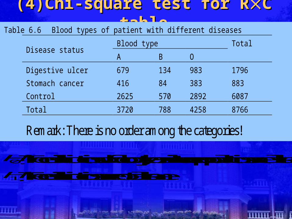
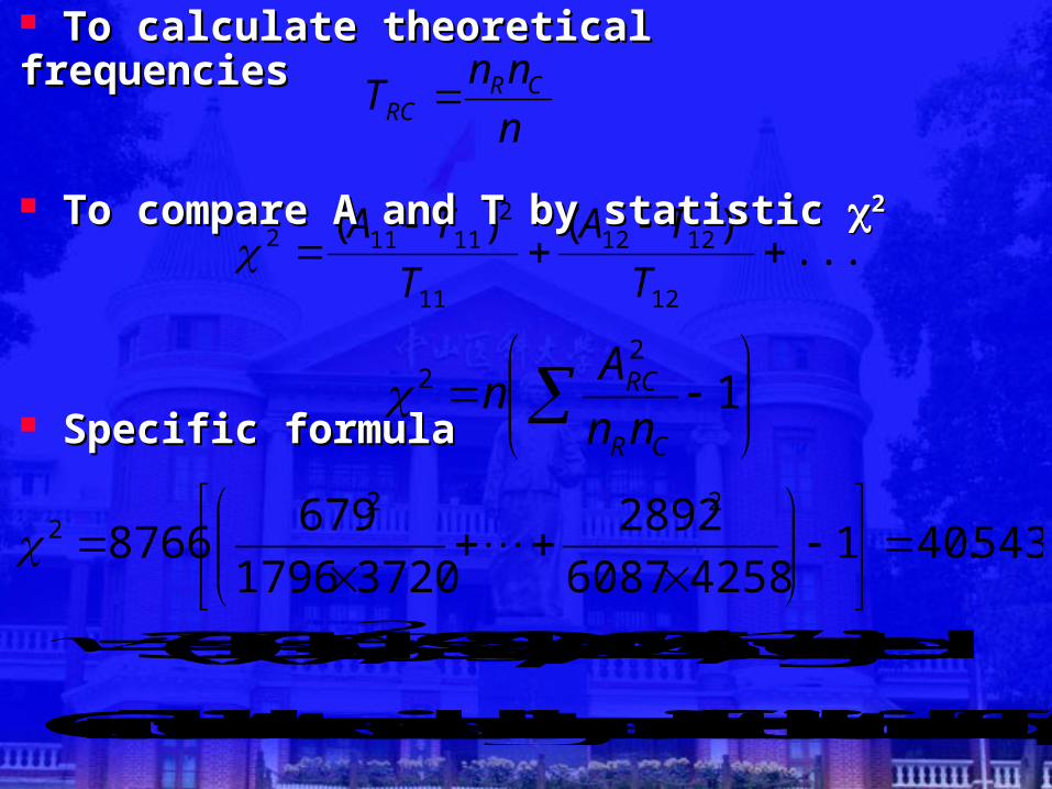
(4)Chi-square test for R(4)Chi-square test for RC tableC tableTable 6.6 Blood types of patient with different diseases

Blood type Total Disease status

A B O

Digestive ulcer 679 134 983 1796

Stomach cancer 416 84 383 883

Control 2625 570 2892 6087

Total 3720 788 4258 8766

Remark: There is no order among the categories!

0H: The distributions of blood types in three populations are all same

1H: The distributions are not all same

n

nnT CR

RC

......)()(

12

21212

11

211112

T

TA

T

TA

To calculate theoretical frequenciesTo calculate theoretical frequencies

To compare A and T by statistic To compare A and T by statistic 22

Specific formulaSpecific formula

1

22

CR

RC

nn

An

543.40142586087

2892

37201796

6798766

222

= (3–1) (3–1) =4, 205.0=9.488 , p＜0.05 , 0H is rejected.

Conclusion: the three diseases might have different distributions of blood type

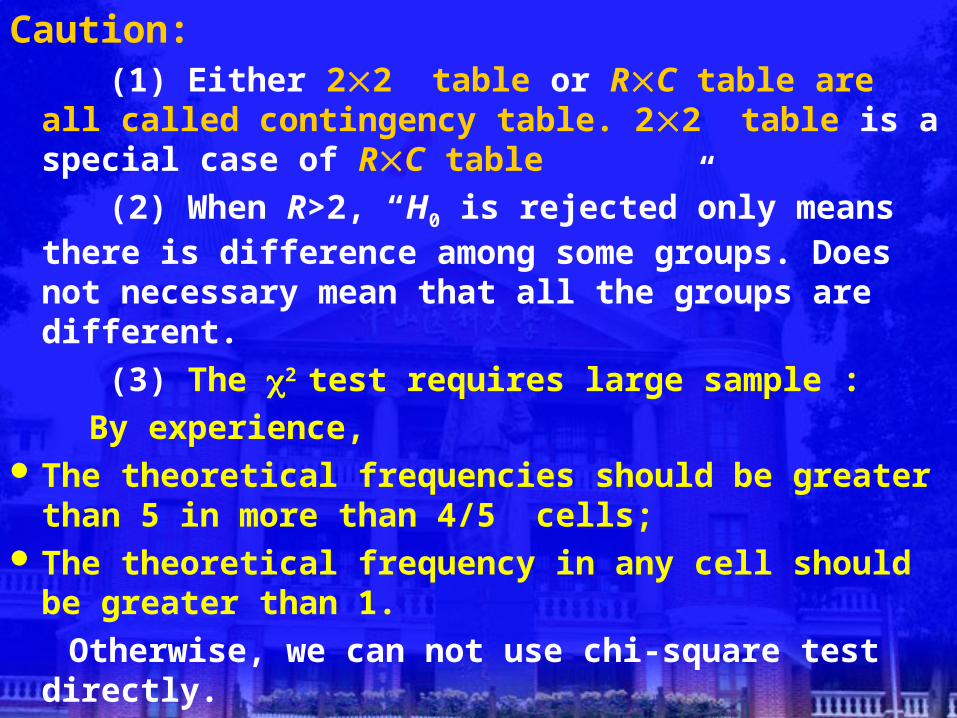
Caution: (1) Either 22 table or RC table are all

called contingency table. 22 table is a special case of RC table

(2) When R>2, “H0 is rejected”only means there is difference among some groups. Does not necessary mean that all the groups are different.

(3) The 2 test requires large sample :

By experience, The theoretical frequencies should be greater than 5 in more

than 4/5 cells; The theoretical frequency in any cell should be greater than

1.

Otherwise, we can not use chi-square test directly.

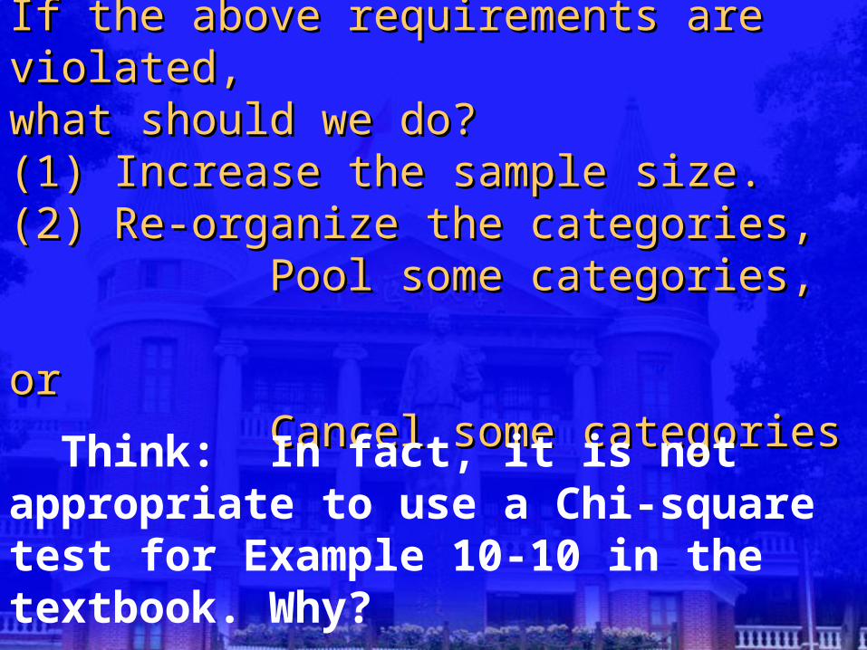
If the above requirements are violated, If the above requirements are violated, what should we do?what should we do?(1) Increase the sample size.(1) Increase the sample size.(2) Re-organize the categories, (2) Re-organize the categories, Pool some categories, Pool some categories, oror Cancel some categories Cancel some categories

Think: In fact, it is not appropriate to use a Chi-square test for Example 10-10 in the textbook. Why?