Embed Size (px)
Citation preview

This thesis has been submitted in fulfilment of the requirements for a postgraduate degree
(e.g. PhD, MPhil, DClinPsychol) at the University of Edinburgh. Please note the following
terms and conditions of use:
• This work is protected by copyright and other intellectual property rights, which are
retained by the thesis author, unless otherwise stated.
• A copy can be downloaded for personal non-commercial research or study, without
prior permission or charge.
• This thesis cannot be reproduced or quoted extensively from without first obtaining
permission in writing from the author.
• The content must not be changed in any way or sold commercially in any format or
medium without the formal permission of the author.
• When referring to this work, full bibliographic details including the author, title,
awarding institution and date of the thesis must be given.

Non-Concave and Behavioural
Optimal Portfolio Choice Problems
Andrea Soa Meireles Rodrigues
Doctor of Philosophy
The University of Edinburgh
2014

c© Andrea Soa Meireles Rodrigues 2014
Some Rights Reserved
This work is licensed under the Creative Commons Attribution-NonCommercial-NoDerivs 3.0 Unported
License. To view a copy of this license, visit http://creativecommons.org/licenses/by-nc-nd/3.0/
or send a letter to Creative Commons, 444 Castro Street, Suite 900, Mountain View, California, 94041,
USA.

Declaration
This thesis, which was composed by myself, is submitted to The University of Edinburghin partial fullment of the requirements for the degree of Doctor of Philosophy in theSchool of Mathematics.
I hereby declare that the work presented in this thesis is, to the best of my knowledgeand belief, original and my own, except where explicitly stated otherwise in the text.I further assert that none of the material contained in this thesis has been submitted,either in part or whole, for any other degree or professional qualication.
Andrea Soa Meireles RodriguesEdinburgh, 30th April 2014

Não me esqueci de nada, mãe.
Guardo a tua voz dentro de mim.Eugénio de Andrade, from `Poema à Mãe' (ll. 3536),
in Os Amantes Sem Dinheiro (1950).
I have not forgotten anything, mother.
I keep your voice inside of me.

Abstract
Our aim is to examine the problem of optimal asset allocation for investors exhibiting
a behaviour in the face of uncertainty which is not consistent with the usual axioms of
Expected Utility Theory. This thesis is divided into two main parts.
In the rst one, comprising Chapter II, we consider an arbitrage-free discrete-time
nancial model and an investor whose risk preferences are represented by a possibly non-
concave utility function (dened on the non-negative half-line only). Under straightfor-
ward conditions, we establish the existence of an optimal portfolio.
As for Chapter III, it consists of the study of the optimal investment problem within
a continuous-time and (essentially) complete market framework, where asset prices are
modelled by semi-martingales. We deal with an investor who behaves in accordance
with Kahneman and Tversky's Cumulative Prospect Theory, and we begin by analysing
the well-posedness of the optimisation problem. In the case where the investor's utility
function is not bounded above, we derive necessary conditions for well-posedness, which
are related only to the behaviour of the distortion functions near the origin and to that
of the utility function as wealth becomes arbitrarily large (both positive and negative).
Next, we focus on an investor whose utility is bounded above. The problem's well-
posedness is trivial, and a necessary condition for the existence of an optimal trading
strategy is obtained. This condition requires that the investor's probability distortion
function on losses does not tend to zero faster than a given rate, which is determined
by the utility function. Provided that certain additional assumptions are satised, we
show that this condition is indeed the borderline for attainability, in the sense that, for
slower convergence of the distortion function, there does exist an optimal portfolio.
Finally, we turn to the case of an investor with a piecewise power-like utility function
and with power-like distortion functions. Easily veriable necessary conditions for well-
posedness are found to be sucient as well, and the existence of an optimal strategy is
demonstrated.
Keywords: Attainability ; Behavioural nance ; Choquet integral ; Dynamic program-
ming ; Finite horizon ; Non-concave utility ; Optimal portfolio ; Probability distortion ;
Well-posedness.
American Mathematical SocietyMathematics Subject Classication (2010):
91G10 (Primary), 49J55 ; 49L20 ; 60H30 ; 91B16 ; 91G80 ; 93E20 (Secondary).
v

Lay summary
A standard problem in the literature of nancial mathematics is that of choosing the best
investment in the assets traded in the market. This optimal portfolio choice problem
has been widely studied under the assumptions of Expected Utility Theory (henceforth
abbreviated to EUT), which assumes in particular that all investors are averse to risk
and that their risk preferences can be represented by a globally concave function, named
utility.
Throughout the years, as many of EUT's key axioms have been challenged by para-
doxes and experiments, various substitute theories for decision making in the face of
uncertainty have been elaborated, such as Cumulative Prospect Theory (CPT). Within
this framework, the existence of a reference point dening gains and losses is assumed,
a feature that is absent in EUT. Moreover, the utility function is now assumed to have
an S -shape, because even though investors generally exhibit risk aversion on gains, they
tend to become risk-seeking when undergoing losses. Lastly, according to CPT, eco-
nomic agents in the real world nd it hard to evaluate the real probabilities of events,
and instead perceive them in a biased way (which is modelled with so-called distortion
functions).
This work presents a study of the portfolio optimisation problem for investors whose
behaviour is not in agreement with the basic tenets of EUT. In the rst part we treat the
case of an investor with a non-concave utility (in a market where trading occurs only at
a nite number of dates), whereas in the second part we incorporate the reference point
and the distortion functions as well (in a market in which assets are traded continuously).
The latter part in particular involves a considerable degree of complexity, especially
since many of the most common mathematical tools used to solving the EUT portfolio
problem are not suitable anymore.
vi
Acknowledgements
To be great, be whole: excludeNothing, exaggerate nothing that is you.
Be whole in everything. Put all you areInto the smallest thing you do.
The whole moon gleams in every pool,It rides so high.
Ricardo Reis, `To be great, be whole', in Odes,tr. and ed. by E. Honig and S.M. Brown
(Poems of Fernando Pessoa, 1986).
More than ten years later, as I face these written pages, I remember that distant daywhen this thesis was born. I cannot think of a more perfect beginning to a piece ofwork, especially when it is that of years which were far from being of solitude. But letus not get ahead of the story.
The great Fernando Pessoa once wrote that `God wills, man dreams, the work isborn.'1 So, with sixteen years of age and a very clear picture in my mind of who Iwanted to be when I grew up, I decided to plan the whole rest of my life. As carefullyand thoroughly as if it were one of my trip itineraries. Of course, I did not care muchabout randomness at that time; life can be funny that way. That is beside the point,though. Adapting Descartes, we can say that, on that day, this thesis was dreamed,therefore it was born.
That was the day that marked the beginning. Today, more than ten years later, asI face the beginning of the end written on these pages, I cannot help but remember thejourney that brought me here. And I realise how long and demanding and sometimesintimidating it was. But solitude, that I cannot nd, for I have been most fortunate inthe people whose paths have intersected mine.
Starting with my rst PhD supervisor, Dr Miklós Rásonyi, without whose guidance,wisdom, patience and encouragement this work would not have been done. I could writehere how thankful I will always be to him for introducing me to a fascinating problem,for his help and concern and words of advice, for his understanding and generosity, foreverything I was able to learn from him. But that would come short of showing thedepth of my gratitude. So, instead, I shall thank him only (in the hope that it will sumit all up) for inspiring me, by example, to continue the pursuit of becoming not only abetter mathematician, but also a better person. All of that while keeping in mind that`le mieux est l'ennemi du bien'.2 And that I should take as many walks as possible.
There have been many other great people who have inuenced and motivated meduring the course of my academic life, from my high-school Mathematics teacher (who,without knowing, awoke in me the wish to become a mathematician) to my universityprofessors (whose engaging lectures only reinforced my belief that I could not have
1`Deus quer, o homem sonha, a obra nasce.' from `O Infante' (l. 1), in Mensagem (1934).2Voltaire, from `La Bégueule: conte morale' (1772, l. 2).
vii

Acknowledgements
made a better choice). In particular, I am extremely obliged to Prof. João Pedro Nunesand to Prof. Isabel Simão, and it is not an overstatement to say that I would not bewhere I am today if it had not been for them. The Probability and Stochastic Analysisresearch group at the School of Mathematics at the University of Edinburgh also deservemy sincerest thank you, as it has been a privilege to be part of such a welcoming,gracious and supporting group. I am truly indebted as well to our Graduate SchoolAdministrator, Mrs Gill Law, for always being so kind, understanding and helpful.
Moreover, I would like to gratefully acknowledge the nancial support providedby FCTFundação para a Ciência e Tecnologia (Portuguese Foundation for Scienceand Technology) through the Doctoral Grant SFRH/BD/69360/2010, without which itwould have been impossible for me to pursue my PhD dream. It can be alarmingly easyto take certain things for granted, so I hope never to forget how blessed I was for beingraised in a country where the basic right to education is no longer reserved for only afew. I pray that no political or economic interests can ever force us to regress.
I would now like to address a heartfelt word of gratitude to all the people whoconstantly remind me that Mathematics is a wonderful part of life, but not the wholeof life's wonders.
Such as my Portuguese friends back home, who despite the 2000 or so kilometresthat separate Lisbon from Edinburgh, have stuck with me all these years. I could nothave asked for better people with whom to grow up. You are my yesterday, my today,and I hope my tomorrow too. With new and obviously hilarious Math jokes.
Such as the Portuguese friends I have met in Edinburgh, who have brought a littlebit of home to an initially foreign land. Thank you for everything we have shared, fromthe cod to the language mishaps, from the fado and football to the saudade. I havebeen so blessed that I have even won a new godmother and a new nephew.
Last, but most certainly not least, such as the non-Portuguese friends I was luckyto make here. In addition to beautiful places, Scotland is also full of beautiful people.
Edina! Scotia's darling seat!. . . . . . . . . . . . . . . . . . . . . . . . . . .Thy sons, Edina, social, kind,With open arms the stranger hail;
Robert Burns, from Address to Edinburgh (1786, ll. 1, 1718)
You were the ones who, in time, made leaving home feel like coming home. Thankyou for enlarging my world, for giving me more reasons and occasions to celebrate, forbringing new words, music and avours into my life. Knowing you has made me richer.
All in all, I wish to thank each and every one of my friends for everything we havelived together. And I do not just mean the big things, but the small ones as well, for it isof those that the `spectacle of the world'3 is made. So thank you! Asante! Dhanyavad!Dòjeh! Efharistó! Gracias! Grazie! Istuti! Köszönöm! Merci! Shukriya! Tak! Te³ekkürederim! Xièxie! Obrigada!4
I must also mention my stronghold, my xed point in life, my adorably crazy family,who love me with all my aws and despite them.
A very special thank you is due to my solid, remarkable grandparents. I could notbe more proud of whom I come from. In a time when life was already dicult enough,they made it a point that their children, and later their children's children, should beraised to become righteous and accomplished people. From them we all learned dignity
3From `Sábio é o que se contenta com o espectáculo do mundo' (l. 1) by Ricardo Reis, in Odes.4Special thanks to Alison for proofreading these Acknowledgements and for precious suggestions.
viii

Acknowledgements
and humility5, the value of everything and everyone, the importance of hard work andthe power of perseverance. You did well. I may not listen to the rosary every day orbe a `home-fairy' yet, but trust me when I say that you did very well and that I cannotthank you enough for that. You can nally call me `doctor', avó!
Secondly, I am very grateful for my cousins. I look at us all grown up and I cannothelp but still see the children we used to be. You are the closest thing I have to siblingsand you made my childhood a magical time. I will never be able to remember Jeuxsans Frontières, Ken dolls, Tamagotchi toys, metal detectors, playing catch or stargazingwithout smiling the widest smile. Thank you for all the singing, ghting and laughing.The only thing I know in life which is as good as having old cousins is having new ones.
My third, and undoubtedly greatest, debt of gratitude goes to my godparents, Elviraand Manuel. I could give here a truly wonderful description of them, but these pagesare too small to contain it. So thank you for being part of the best and worst momentsof my life. You are both so incredibly good and generous to me that, if I did not knowyou are real, I would say that godparents like you could only exist in fairy tales.
Finally (I always like to save the best things for last, like a dessert), I wish to thankIsabel, my pillar of a mum. Thank you for being a model of strength, determination,commitment. And constancy, you know how much that means to me. Besides, whenalmost everyone was trying to convince me to go to medical school (fainting is clearlyoverrated), thank you for supporting my seemingly eccentric dream of becoming a math-ematician (without ever giving me the slightest hint that you were less proud of me forthat). Better yet, thank you for supporting all my dreams. Thank you for all the timesyou are strict and for all the times you spoil me. For being such a demanding and givingperson. For every soup. Thank you, not only for your unshakable faith in me, but alsofor never letting me settle for less than what you believe I am capable of accomplishing.
Recomeça. . .Se puderes,Sem angústia e sem pressa.. . . . . . . . . . . . . . . . . . . . . . . . . . .Enquanto não alcancesNão descanses.De nenhum fruto queiras só metade.
Miguel Torga, from Recomeça (ll. 13, 810)
Start again. . .If you can,Without anguish and without haste.. . . . . . . . . . . . . . . . . . . . . . . . . . . . . . . . . . . .Until you reach [your goal]Do not rest.Of no fruit should you want only half.
Thank you for being the push that I need every time I resist ying solo. And for beingmy safety net (I never have to look down to be sure that you are there). Thank you somuch for a love which helps me grow without smothering me (unlike mine for my cacti).I know it is a very small thing when compared to everything you have given me, but thisthesis is for you. Of course, by now you must be thinking that these acknowledgementshave already too many words, but the truth is that they will always have too few. So Ishall nish by simply saying obrigada, mãe. For everything. I owe you all that I am.
To conclude, I would like to remark that `the soul is divine and the work is imper-fect.'6 Thus, any errors or omissions which may remain in the content of this thesis aresolely my responsibility. `All else is up to God!'7
5`Perfection is impossible without humility. Why should I strive for perfection, if I am already goodenough?', by Leo Tolstoy, in A calendar of wisdom: daily thoughts to nourish the soul, tr. and ed. byP. Sekirin (2010).
6`A alma é divina e a obra é imperfeita.', from `Padrão' (l. 5) by Pessoa, in Mensagem (1934).7`Tudo o mais é com Deus!', from `D. Pedro' (l. 12) by Pessoa, in Mensagem (1934).
ix
Contents
Abstract v
Lay summary vi
Acknowledgements vii
Contents x
List of gures xii
List of abbreviations xiii
List of symbols xiv
I Introduction and summary 1
I.1 Introduction . . . . . . . . . . . . . . . . . . . . . . . . . . . . . . . . . . 1I.2 Summary . . . . . . . . . . . . . . . . . . . . . . . . . . . . . . . . . . . 3
II Non-concave portfolio optimisation 5
II.1 Introduction . . . . . . . . . . . . . . . . . . . . . . . . . . . . . . . . . . 5II.2 Notation and set-up . . . . . . . . . . . . . . . . . . . . . . . . . . . . . 6
II.2.1 The market . . . . . . . . . . . . . . . . . . . . . . . . . . . . . . 6II.2.2 The investor . . . . . . . . . . . . . . . . . . . . . . . . . . . . . . 11II.2.3 The optimal portfolio problem . . . . . . . . . . . . . . . . . . . 13II.2.4 Toy example: one-period binomial model . . . . . . . . . . . . . . 15
II.3 Optimal strategy in the one-step case . . . . . . . . . . . . . . . . . . . . 17II.4 Dynamic programming . . . . . . . . . . . . . . . . . . . . . . . . . . . . 22II.5 Proofs and auxiliary results . . . . . . . . . . . . . . . . . . . . . . . . . 24
II.5.1 Auxiliary results . . . . . . . . . . . . . . . . . . . . . . . . . . . 24II.5.2 Proofs of Section II.2 . . . . . . . . . . . . . . . . . . . . . . . . . 30II.5.3 Proofs of Section II.3 . . . . . . . . . . . . . . . . . . . . . . . . . 31II.5.4 Proofs of Section II.4 . . . . . . . . . . . . . . . . . . . . . . . . . 59
III Behavioural portfolio optimisation 68
III.1 Introduction . . . . . . . . . . . . . . . . . . . . . . . . . . . . . . . . . . 68III.2 Notation and set-up . . . . . . . . . . . . . . . . . . . . . . . . . . . . . 72
III.2.1 The market . . . . . . . . . . . . . . . . . . . . . . . . . . . . . . 72III.2.2 The investor . . . . . . . . . . . . . . . . . . . . . . . . . . . . . . 74III.2.3 The optimal portfolio problem . . . . . . . . . . . . . . . . . . . 77III.2.4 Toy example: one-period binomial model (revisited) . . . . . . . 79
III.3 General results in continuous time . . . . . . . . . . . . . . . . . . . . . 81
x

Contents
III.3.1 Feasible portfolios . . . . . . . . . . . . . . . . . . . . . . . . . . 84III.3.2 Well-Posedness . . . . . . . . . . . . . . . . . . . . . . . . . . . . 84III.3.3 Attainability . . . . . . . . . . . . . . . . . . . . . . . . . . . . . 90III.3.4 Examples . . . . . . . . . . . . . . . . . . . . . . . . . . . . . . . 91
III.4 Bounded utility on gains . . . . . . . . . . . . . . . . . . . . . . . . . . . 94III.4.1 Feasible portfolios . . . . . . . . . . . . . . . . . . . . . . . . . . 94III.4.2 Well-posedness . . . . . . . . . . . . . . . . . . . . . . . . . . . . 95III.4.3 Attainability . . . . . . . . . . . . . . . . . . . . . . . . . . . . . 95
III.5 Power utilities and distortions . . . . . . . . . . . . . . . . . . . . . . . . 98III.5.1 Well-posedness . . . . . . . . . . . . . . . . . . . . . . . . . . . . 99III.5.2 Attainability . . . . . . . . . . . . . . . . . . . . . . . . . . . . . 101
III.6 Proofs and auxiliary results . . . . . . . . . . . . . . . . . . . . . . . . . 102III.6.1 Auxiliary results . . . . . . . . . . . . . . . . . . . . . . . . . . . 102III.6.2 Proofs of Section III.3 . . . . . . . . . . . . . . . . . . . . . . . . 109III.6.3 Proofs of Section III.4 . . . . . . . . . . . . . . . . . . . . . . . . 116III.6.4 Proofs of Section III.5 . . . . . . . . . . . . . . . . . . . . . . . . 117
IV Conclusions and future work 120
Appendices 122
A Asymptotic elasticity . . . . . . . . . . . . . . . . . . . . . . . . . . . . . 122B Measure theory . . . . . . . . . . . . . . . . . . . . . . . . . . . . . . . . 124
B.1 General results . . . . . . . . . . . . . . . . . . . . . . . . . . . . 124B.2 Cumulative distribution function and quantile function . . . . . . 125
C Choquet integral . . . . . . . . . . . . . . . . . . . . . . . . . . . . . . . 127
References 129
Index 134
First Supervisor
Dr Miklós Rásonyi, MTA Alfréd Rényi Institute of Mathematics, Hungary; andSchool of Mathematics, The University of Edinburgh, Scotland, U.K..
Examiners
I wish to thank
(External) Dr Beatrice Acciaio, Department of Statistics, The London School ofEconomics and Political Science, U.K.,
(Internal) Dr Sotirios Sabanis, School of Mathematics, The University of Edin-burgh, Scotland, U.K.,
for kindly agreeing to be my examiners, and for providing excellent corrections andimprovements to this thesis.
Manuscript's history
Submitted for examination: 30th April 2014,Defended (viva voce): 30th June 2014.
xi

List of gures
II.1 EUT v. non-concave portfolio choice problems . . . . . . . . . . . . . . . 16
III.1 Non-concave behavioural portfolio choice problem . . . . . . . . . . . . . 80
III.2 Ill-posed behavioural portfolio choice problem . . . . . . . . . . . . . . . 81
III.3 Non-attainable behavioural portfolio choice problem . . . . . . . . . . . 81
xii

List of abbreviations
(NA) Arbitrage-free condition
a.e. Almost everywhere or almost every
a.s. Almost surely
AE Asymptotic elasticity
CDF Cumulative distribution function
CPT Cumulative Prospect Theory
càdlàg Right-continuous with left-limits
(from the French continu(e) à droite, limité(e) à gauche)
DP Dynamic programming
E(L)MM Equivalent (local) martingale measure
EUT Expected Utility Theory
HJB Hamilton-Jacobi-Bellman
LLAD Large-loss aversion degree
NFLVR No free lunch with vanishing risk
PDE Partial dierential equation
r.v. Random variable
RAE Reasonable asymptotic elasticity
SDE Stochastic dierential equation
xiii

List of symbols
, means that the expression on the left is dened to be equal to the expression on the
right
General notation
11X indicator function of the set X⊔pairwise disjoint union
function composition
cl (X) topological closure of the set X
3 indicates the end of a remark
d·e (respectively, b·c) ceiling function (respectively, oor function)
〈·, ·〉Rn Euclidean inner product
‖·‖Rn Euclidean norm
log denotes the natural logarithm
Bn (x0, r) , x ∈ Rn: ‖x− x0‖Rn < r open ball of centre x0 ∈ Rn and radius r > 0
sgn signum function
P (X) power set of X, i.e., the collection of all subsets of X
R , R ∪ −∞,+∞ = [−∞,+∞] extended real number line
end of proof (or Halmos) mark
> (superscript) matrix transposition
∅ , empty set
0n null vector of Rn
∨ (respectively, ∧) maximum operator (respectively, minimum operator), i.e., x ∨ y ,max x, y (respectively, x ∧ y , min x, y) for any x, y ∈ RAE+ (f) asymptotic elasticity of the function f
Ef (x) elasticity of the function f at the point x
f (+∞) limit (if it exists) of the real-valued function f as x→ +∞x+ , max x, 0 (respectively, x− , −min x, 0) for every x ∈ RXc complement set of X
Measure theory
` Lebesgue measure on Ress supf∈Θ f (respectively, ess inff∈Θ f) essential supremum (respectively, essential in-
xiv

List of abbreviations
mum) of the family Θ of measurable functions
ess supµ f (respectively, ess infµ f) essential supremum (respectively, essential inmum)
of the function f with respect to the measure µ∫X f dµ Lebesgue integral of f with respect to the measure µ
B (S) Borel σ-algebra of the topological space (S, τ)
PX|G regular conditional distribution of the function X given the σ-algebra G , under
the probability measure Psupp (µ) topological support of the measure µ
C
∫X f dµ Choquet integral of f with respect to the capacity µ
ProjX (E) , x ∈ X: ∃ y ∈ Y such that (x, y) ∈ E projection of E ⊆ X × Y on X
F PX (respectively Fµ) cumulative distribution function of the r.v. X with respect to the
probability measure P (respectively, of the probability measure µ on (R,B (R)))
L0 (X,Σ, µ) vector space of (equivalence classes of) measurable functions f : X → RLp (X,Σ, µ) vector space of (equivalence classes of) functions f ∈ L0 (X,Σ, µ) verifying∫X |f |
p dµ < +∞ (with p ∈ (0,+∞))
qPX (respectively, qµ) quantile function of the r.v. X with respect to the probability
measure P (respectively, of the probability measure µ on (R,B (R)))
UP∼ U (I) means that the r.v. U has a (continuous) uniform distribution on the non-
degenerate interval I ⊆ R with respect to the probability measure P
Convex analysis
aff (X) ane hull of the set X
conv (X) convex hull of the set X
E (X) set of extreme points of the set X
lin (X) linear span of the set X
ri (X) relative interior of the set X
Multi-functions
dom S , x ∈ X: S (x) 6= ∅ domain of the multi-function S
gph S , (x, y) ∈ X × Rn: x ∈ dom S and y ∈ S (x) graph of the multi-function
S
S : X ⇒ Rn multi-function from the set X to the Euclidean space Rn
S −1 (U) , x ∈ X: S (x) ∩ U 6= ∅ inverse image under the multi-function S of the
set U ⊆ Rn
Financial mathematics
βt, κt see Proposition II.2.11
∆St , St − St−1 (or ∆St , St − St−)F ltration describing the information accruing to the agents in the economy
P physical probability
P∗ ELMM
xv

List of symbols
A (x0) set of feasible portfolios
Me (S) (respectively, M loce (S)) set of all EMM (respectively, all ELMM )
W class of real-valued random variables with nite moments of all (positive) orders,
see eq. (II.4.5)
Ω sample space, that is, set of all possible market scenarios
Ωt see page 10
φ portfolio
φ∗optimal portfolio
ϕx0trivial portfolio
Φ (respectively, Φ (x0)) class of self-nancing portfolios (respectively, starting from ini-
tial capital x0)
Πφ wealth process of the portfolio φ
Ψ (respectively, Ψ (x0)) set of all admissible strategies (respectively, for the initial cap-
ital x0)
ρ , dP∗/dP state price density
Ωt see Proposition II.2.10
Ξdt−1 see page 10
S , S/S0 discounted value process of S
Ξdt−1 (H) (or Ξdt−1 (x)), see page 10
Ξnt family of all Ft-measurable, Rn-valued random vectors
Dt (ω) see page 10
M (x) see Lemma II.5.8
M (x) , Z (x) see Lemma II.5.9
S price process of the risky assets
S0 price process of the riskless asset
T trading horizon
u utility function
u+ (respectively, u−) utility on gains (respectively, on losses)
V (X) prospect functional of the random variable X, see Denition III.2.10
v∗ (x0) supremum of the optimal portfolio problem
V± (X) Choquet integrals of the random variable X, see eq. (III.2.7)
x0 investor's initial capital
r spot rate process
xvi
Chapter I
Introduction and summary
1 Introduction
It seems reasonable to assume that any economic agent possessing a certain amount
of wealth wishes to invest it in the most favourable way. Finding the most desirable
investment strategies is precisely in what consists the optimal portfolio choice problem,
a classic one in the eld of nancial mathematics.
A natural question that instantly arises concerns the criteria governing the investors'
choices. After the ground-breaking work of Bernoulli [10], and ever since the seminal
papers of Merton [39, 40] and Samuelson [55], Expected Utility Theory appears to have
been one of the predominantly used theories in the literature for modelling decision mak-
ing under uncertainty. This theory, also commonly known as EUT, was formulated by
von Neumann and Morgenstern [62], and states that every rational investor's individual
preferences (formally described by a binary relation satisfying certain properties) can
be numerically measured and represented by a function, called utility (for a thorough
treatment of this subject, the interested reader is referred e.g. to Föllmer and Schied
[25, Sections 2.12.3]). Then, assuming that there is no intermediate consumption and
that the investment horizon is nite, within this framework the investors will always
choose a portfolio whose terminal value maximises their expected utility.
Dierent investors are allowed to possess dierent utilities, but it is assumed that
these functions must all satisfy some common basic properties, with well-established
economic meanings.
Firstly, the domain of the real-valued von Neumann-Morgenstern utility function has
to include all possible outcomes of investment. For example, when wealth is restricted
to be non-negative, the utility can be taken to be dened on the positive half-line only,
whereas in the case where wealth is allowed to become negative, the domain must consist
of the whole real line.
Moreover, every utility should be strictly increasing in wealth, to translate the fact
that investors are greedy and non-satiable (or equivalently, their preference relations
are monotone), that is, more is always better than less and no agent will ever have so
1
Chapter I. Introduction and summary 1. Introduction
much wealth that getting more would not be at least a little bit desirable.
In addition, the utilities are assumed to be continuous, because small modications
in wealth should have small impacts on preferences.
While these assumptions tend to be more or less undisputed, there is another one
regarding the shape of the utility which has been met with a great deal of criticism,
as we shall see below. Indeed, EUT postulates that all investors are risk-averse in the
face of uncertainty at all times, which is reected by a globally concave utility (so the
marginal utility of wealth decreases as wealth increases).
Finally, according to EUT, all investors are completely rational and fully capable of
objectively assessing probabilities.
Now, this theory is particularly appealing and relatively simple in that there exists
a great variety of tools which can be employed for solving the portfolio optimisation
problem.
One of the main approaches makes use of the dynamic programming (DP) principle,
which roughly speaking allows for the problem to be broken into two related problems
over two time intervals, the aim being to determine the optimal decision at each stage
so that the resulting combined decision is globally optimal (we refer e.g. to Pham [44,
Chapter 3]). This principle, whose proof relies not only on a Markov assumption on
the asset prices and on measurable selection theorems, but also on the the dynamic
consistency (or tower property) of the conditional expectation, is invoked to derive
(through an application of Itô's formula) a partial dierential equation (PDE), known
in the literature as the Hamilton-Jacobi-Bellman (HJB) equation. Then, after obtaining
a smooth solution (or showing its existence) by PDE methods, one concludes by checking
that this smooth solution is indeed the value function of the optimisation problem (this
is called the verication step, which again makes use of Itô's formula and gives, as a
by-product, an optimal trading strategy).
Another common approach, which is more general (in the sense that it has weaker
assumptions), involves martingale theory and convex duality techniques. The basic
idea is the following: by appealing to the Itô martingale representation theorem, the
original portfolio problem is transformed into a static optimisation problem subject
to a linear budget constraint. Given that the utility function is globally concave, we
are dealing with a concave maximisation problem, therefore we can apply methods of
convex analysis to formulate and solve a dual problem, which in turn gives the solution
to the primal problem (for a detailed account of this theory in continuous-time markets
where prices are modelled by Itô processes, see for example Karatzas and Shreve [32,
Chapter 3] and the references therein).
EUT has had several important applications, ranging from portfolio optimisation,
to indierence pricing (thus providing an important method for valuing non-hedgeable
claims) and to the theory of risk measures (a famous one being the entropic risk measure,
which is associated with the exponential utility function).
However, over the years, some of EUT's fundamental principles have been systemati-
2

Chapter I. Introduction and summary 2. Summary
cally questioned by several paradoxes (e.g., Allais [2] paradox and Ellsberg [23] paradox)
and empirical studies. Namely, the latter have demonstrated that decision makers do
not evaluate wealth in terms of nal asset states, but with respect to a reference point
(which denes gains and losses). Also, whilst the investors are generally risk-averse
on gains, they were found to exhibit a risk-seeking behaviour when making decisions
involving losses. Furthermore, in reality, the economic agents are subjective and have
a distorted perception of the actual probabilities (for example, small probabilities tend
to be exaggerated, which may not only explain the Allais paradox, but also the attrac-
tiveness of insurance and gambling, as remarked for instance in Kahneman and Tversky
[31]).
The attempts to incorporate the above psychological ndings into economic theory
have lead to the emergence of several alternative theories, amongst which is the Prospect
Theory proposed by Kahneman and Tversky [31] (later amended in Tversky and Kahne-
man [61] to ensure that rst order stochastic dominance is not violated1, and re-named
Cumulative Prospect Theory or CPT for short). The main tenets of this theory, for
which Kahneman was awarded the Nobel Memorial Prize in Economics in the year 2002,
are essentially the following: rstly, the existence of a reference point for each investor;
secondly, the consideration of a utility function (now called prospect value function),
dened on the real line, which is S -shaped (that is, concave and convex on the positive
and negative half-lines, respectively); lastly, the use of probability weighting functions
to model the way in which the investors miscalculate the physical probability measure
(leading to the appearance of possibly non-linear Choquet [17] integrals). These make
the study of the portfolio problem within the CPT framework substantially dierent
from that of the EUT portfolio problem.
In this work, we shall therefore investigate the nite-horizon optimal portfolio prob-
lem for investors who violate the axioms of EUT, namely for a rational investor with a
non-concave utility function in a discrete-time nancial market, as well as for an agent
behaving consistently with CPT in a continuous-time model.
2 Summary
A brief outline of this work is as follows.
Chapter II treats the discrete-time asset allocation problem when the investor has a
non-concave utility function and when wealth is restricted to remain non-negative. In
Section II.1 we present a short overview of some of the relevant literature on the subject.
Section II.2 is dedicated to briey recalling some of the basic concepts and results. In
particular, the market model is specied, which is followed by the rigorous description of
1That is, an investor will choose a portfolio over another if the terminal value of the latter issecond-order stochastically dominated by the terminal value of the former. We recall that, given aprobability space (Ω,F ,P), the random variable (r.v.) X has rst-order stochastic dominance (re-spectively, second-order stochastic dominance) over the r.v. Y if PX ≥ x ≥ PY ≥ x (respectively,∫ x−∞ (PY ≤ y − PX ≤ y) dy ≥ 0) for all x, with strict inequality for some x, and it is clear thatrst-order stochastic dominance implies second-order stochastic dominance.
3

Chapter I. Introduction and summary 2. Summary
the investor and by the mathematical formulation of the non-concave portfolio problem.
Additionally, we construct a very simple toy example in which we emphasise some of
the dierences to EUT portfolio optimisation. Next, in Section II.3 we examine the
problem in a one-step setting, while in Section II.4 we state our main result, which is
proved using a dynamic programming approach. For the sake of exposition, all auxiliary
results and proofs are compiled in Section II.5.
On the other hand, the topic of Chapter III is the continuous-time asset allocation
problem for a behavioural investor in an essentially complete model. As before, Sec-
tion III.1 provides a brief highlight of some of the existing literature, as well as of the
main challenges of CPT. In the following Section III.2, we introduce a general model,
make precise the tenets of CPT, rigorously state the behavioural portfolio problem, and
return to the toy model of the preceding chapter to illustrate the importance of the
changes introduced by CPT with respect to EUT in the optimisation problem. Then,
in Section III.3, we restrict ourselves to the case of a continuous-time nancial market,
and we lay down the main assumptions which will be in force throughout the remainder
on the chapter. The issues of well-posedness and attainability (see Denitions III.2.16
and III.2.17) are dealt with, and examples are included to demonstrate that the obtained
results hold in important model classes. Moreover, in Section III.4 and Section III.5 we
respectively consider the special cases where the utility on gains is bounded above and
where both the utilities and the distortions are power functions. Once more, to improve
readability, we collect the proofs and the auxiliary results in Section III.6.
Finally, Chapter IV, which concludes the present manuscript, summarises our most
important ndings and contributions, whilst suggesting ideas for further research.
4

Chapter II
Non-concave portfolio optimisation
1 Introduction
The work in this chapter will be the content of the future paper [14].
It focuses on the problem of choosing an optimal strategy for an investor who has
a possibly non-concave utility function, dened on the non-negative half-line only. We
shall be working in a nite-horizon and discrete-time frictionless market setting. Below
is gathered a short description of some of the relevant research conducted in this subject.
Amongst several signicant papers developed within the EUT framework, it is im-
perative to mention that by Kramkov and Schachermayer [35], as well its successor by
Schachermayer [58]. In a continuous-time and not necessarily complete market model
where it is assumed that asset prices are modelled with locally bounded semi-martingales
and that the set of equivalent local martingale measures is non-empty, both papers show
the existence of a solution to the optimal portfolio problem, provided that a certain con-
dition involving the asymptotic elasticity of the utility is satised (famously named the
reasonable asymptotic elasticity condition). This is accomplished via well-known tools
of convex analysis. We further recall that, while in the rst paper the utility is dened
on the non-negative axis (for wealth is constrained to remain non-negative), the domain
of the utility in the latter one is the whole real line. Despite their unquestionable im-
portance, both papers, however, apply only to utility functions which are concave and
smooth enough.
With regard to discrete-time and also possibly incomplete market models, we would
like to point out the work of Rásonyi and Stettner [50] for a utility function on the
whole real line, which is complemented by the paper [51] by the same authors for a
utility on the non-negative half-line. In both cases, the existence of an optimal strategy
is proved, this time by exploiting a dynamic programming technique. Moreover, weaker
asymptotic elasticity conditions are imposed, and neither the smoothness of the utility
nor the boundedness of the asset price processes are required. Yet, as before, the utilities
are supposed to be concave.
A study of the optimal portfolio choice problem for a possibly non-concave and non-
5
Chapter II. Non-concave optimisation 2. Notation and set-up
smooth utility on the whole real line is presented in Carassus and Rásonyi [12]. There,
again by a dynamic programming argument, it is established that a condition on the
growth of the utility (associated with the notion of asymptotic elasticity) is sucient
to ensure that an optimal solution does in fact exist. Our goal here is to complement
this paper, in the sense that we wish to solve the same problem, but for a non-concave
utility whose domain is the non-negative axis (while borrowing ideas from Rásonyi and
Stettner [51]).
In addition, we mention Reichlin [52, Chapter II], who studies the same optimisation
problem for non-concave utility functions on the non-negative half-line which are of
strictly sublinear growth1. Besides proving the existence of an optimal investment
strategy under a condition involving the asymptotic elasticity and using methods of
convex analysis, the author also examines some of its properties. Nonetheless, the
existence result therein is not comparable to ours since, in Reichlin [52], the work
is conducted with respect to a xed martingale measure, whereas we impose some
restrictions (see our Assumption II.2.16).
Finally, we remark that, in all of the aforementioned papers, rather than looking
for conditions ensuring the well-posedness of the optimisation problem (i.e., that its
supremum is nite), the authors simply assume that well-posedness holds true (which,
as they remark, is not enough to imply the existence of an optimal strategy). This
common practice will also be adopted in this chapter (we refer to our equation (II.4.3)).
2 Notation and set-up
2.1 The market
In what follows, we shall consider a frictionless and totally liquid nancial market, that
is, in which all costs and restraints associated with transactions are non-existent, where
investors are allowed to short-sell stocks and to borrow money, and nally where it is
always possible to buy or sell an unlimited number of shares of any asset.
Let the current time be denoted by 0, and let us x a nite trading horizon T ∈ N.We assume further that this is a discrete-time market, that is, that trading occurs only
at nitely many points in time, or trading dates, given by 0, 1, . . . , T.Also, the uncertainty in the economy is characterised by a complete probability space
(Ω,F ,P), with F a σ-algebra on the sample space Ω, and P the underlying probability
measure (to be interpreted as the physical probability) on (Ω,F ). Moreover, all the
information accruing to the agents in the economy is described by a discrete ltration
F = Ft; t ∈ 0, 1, . . . , T such that F0 contains all P-null sets, where the fact that noinformation is lost is expressed by the non-decreasing nature of F. Finally, we assume
for convenience that the σ-algebra F0 is P-trivial2, and also that F = FT .
1A function f : [ 0,+∞) → R is of strictly sub-linear growth if limx→+∞ f(x) /x = 0.2Given a probability space (Ω,F ,P), a σ-algebra G ⊆ F is P-trivial if, for every A ∈ G , either
P(A) = 0 or P(Ω \A) = 0.
6

Chapter II. Non-concave optimisation 2. Notation and set-up
Next, we x some strictly positive integer d, and we consider an Rd-valued (not
necessarily locally bounded) process S = St; t ∈ 0, 1, . . . , T, where St represents theprices at time t of d traded risky assets3. We shall consider as well the existence of a risk-
free asset , also called money market, whose price process S0 =S0t ; t ∈ 0, 1, . . . , T
satises S0
0 = 1 and evolves, as shown below, according to a non-negative spot rate
process r = rt; t ∈ 1, . . . , T,
S0t ,
t∏s=1
(1 + rs) , t ∈ 1, . . . , T ,
where rt is Ft−1-measurable. Then, borrowing the notation4
St ,(S0t , S
>t
)>=(S0t , S
1t , . . . , S
dt
)>, t ∈ 0, 1, . . . , T ,
from Föllmer and Schied [25], and introducing, for each n ∈ N and t ∈ 0, 1, . . . , T, thefamily Ξnt of all Ft-measurable random vectors ξ : Ω→ Rn, we assume that the process
S is adapted to the ltration F, or in other words, St ∈ Ξd+1t for every t ∈ 0, 1, . . . , T.
Note that the adaptedness of the price process translates the fact that the price vector
St is known at time t. In addition, let us designate the quantity(S0t
)−1as the discount
factor at time t, and dene the Rd-valued discounted value process of S as follows,
S =St = St/S
0t ; t ∈ 0, 1, . . . , T
.
Finally, for each t ∈ 1, . . . , T, we dene the Ft-measurable, d-dimensional random
vector ∆St , St − St−1.
We now recall the following.
Denition II.2.1 (Trading strategy). We say that an F-adapted, Rd+1-valued sto-
chastic process φ =φt =
(φ0t , φ>t
)>; t ∈ 1, . . . , T
, with φt =
(φ1t , . . . , φ
dt
)>, is a
trading strategy or portfolio if it is predictable with respect to F, i.e., if it veries
φt ∈ Ξd+1t−1 , ∀ t ∈ 1, . . . , T . (II.2.1)
Then, for every t ∈ 1, . . . , T and i ∈ 0, 1, . . . , d, φit represents the number of shares
of the i-th asset which are held by the investor at time t.
Remark II.2.2. (i) The predictability of the portfolio process means that the positions
in the portfolio for each time t ∈ 1, . . . , T are decided based on the information
available at time t−1, and kept until time t, when the new prices St are revealed.
(ii) We recall that both short-selling and borrowing are allowed, which accounts for
the fact that no constraints are imposed on the sign of φit. 3
3These can be, for example, common stocks, commodities, foreign currencies, exchange rates ormarket indices, to name only a few.
4Here, the superscript > denotes matrix transposition.
7

Chapter II. Non-concave optimisation 2. Notation and set-up
To each portfolio is obviously associated a value, which is naturally dened as shown
below.
Denition II.2.3 (Wealth process). The value of a trading strategy φ at each time
t ∈ 0, 1, . . . , T is given by5
Πφt ,
⟨φ1, S0
⟩Rd+1 = φ0
1 + 〈φ1, S0〉Rd , if t = 0,⟨φt, St
⟩Rd+1 = φ0
tS0t + 〈φt, St〉Rd , otherwise,
(II.2.2)
and we call Πφ =
Πφt ; t ∈ 0, 1, . . . , T
the wealth process of φ. Moreover, we say
that φ starts from initial capital x0 ∈ R if Πφ0 = x0 almost surely (a.s.).
So we can introduce the following important concept.
Denition II.2.4 (Self-nancing). A trading strategy φ is called self-nancing if, for
every t ∈ 1, . . . , T − 1, the equality
Πφt =
⟨φt+1, St
⟩Rd+1 (II.2.3)
holds a.s.. We denote by Φ the class of all self-nancing portfolios, and by Φ(x0) the
class of all self-nancing portfolios starting from initial capital x0 ∈ R.
Remark II.2.5. The self-nancing condition means that, before each time t ∈ 2, . . . , Tand after the prices St−1 are known, the investor adjusts his position from φt−1 to φtwithout injecting or withdrawing any wealth. It can be easily checked that a portfolio
φ is self-nancing if and only if
∀ t ∈ 1, . . . , T , Πφt = Πφ
0 +t∑
s=1
[φ0s
(S0s − S0
s−1
)+ 〈φs,∆Ss〉Rd
]a.s.. (II.2.4)
3
We proceed with the mathematical statement of the notion of arbitrage, which can
be described in lay terms as the opportunity to, out of nothing and without risk, make
a sure prot.
Denition II.2.6 (Arbitrage opportunity). We say that a portfolio φ ∈ Φ(0) is an
arbitrage opportunity if its value process satises both conditions below,
(i) for every t ∈ 1, . . . , T, Πφt ≥ 0 a.s.,
(ii) P
ΠφT > 0
> 0.
In order to keep the notation simple, henceforth we shall suppose, without loss of
generality, that the risk-free asset has constant price, that is, for every t ∈ 1, . . . , Twe have S0
t = 1 a.s. (i.e., the spot rate is null). Hence, we work directly with discounted
prices and, like in Øksendal [43, Denition 12.1.1], we say that the market is normalised .
5We recall that, given x, y ∈ Rn, the Euclidean inner product is dened by 〈x, y〉Rn ,∑ni=1 xiyi.
Moreover, we denote by ‖x‖Rn ,√〈x, x〉Rn the Euclidean norm of x.
8

Chapter II. Non-concave optimisation 2. Notation and set-up
Then, as in Rásonyi and Stettner [51], we shall impose the trading constraint that
the value of a portfolio should not be allowed to become strictly negative.
Denition II.2.7 (Admissibility). Given x0 ≥ 0, we say that a portfolio φ ∈ Φ(x0)
is admissible for x0 if
∀ t ∈ 1, . . . , T , Πφt ≥ 0 a.s.. (II.2.5)
We denote by Ψ(x0) the set of all admissible strategies for x0.
Remark II.2.8. Neither Rásonyi and Stettner [50], nor Carassus and Rásonyi [12] place
any admissibility restriction on the portfolios, and therefore they allow portfolios whose
value processes not only may take strictly negative values with positive probability,
but also are not necessarily bounded from below. We observe, however, that our ad-
missibility condition, despite considerably restricting the set of admissible portfolios
(cf. Remark 2.1 in Carassus and Rásonyi [12]), is frequently adopted in the literature.
Moreover, it is not a completely unreasonable or unrealistic one, as in pratice it means
the existence of a credit limit (strictly negative positions, i.e. debts, are forbidden). 3
Given that, in reality, arbitrage opportunities, when they occur, are immediately
exploited by the investors, and thus tend to be eliminated quickly, it is only natural to
impose the following throughout.
Assumption II.2.9 (Absence of arbitrage). The market is arbitrage-free, that is,
if φ ∈ Ψ(0) , then ΠφT = 0 a.s.. (NA)
Now x t ∈ 1, . . . , T. We know that there exists a regular conditional distribution6
of ∆St with respect to Ft−1, under the physical measure P (see e.g. Theorem 10.2.2 in
Dudley [22, pp. 345346]), which we shall denote by7
P∆St|Ft−1 : B(Rd)× Ω→ [0, 1] .
6Here, 11A : X → 0, 1 denotes the indicator function of a subset A of a set X, dened by
11A(x) ,
1, if x ∈ A,0, otherwise.
Then, letting (Ω,F ,P) be a complete probability space, (S,Σ) be a measurable space, X : Ω→ S bea (F ,Σ)-measurable function, and G ⊆ F be a σ-algebra over Ω containing all P-null sets, we recallthat a regular conditional distribution of X given G , under P, is a function PX|G : Σ× Ω→ [0, 1] forwhich the two conditions below hold true,
(i) for each E ∈ Σ, the function PX|G(E, ·) : Ω→ [0, 1] is measurable with respect to G , and thereexists Ω ∈ G with P
(Ω)
= 1 such that PX|G(E,ω) = EP[11E(X) |G ](ω) for every ω ∈ Ω,
(ii) there is some Ω ∈ G with P(Ω)
= 1 such that, for every ω ∈ Ω, the function PX|G(·, ω) : Σ →[0, 1] is a probability measure on (S,Σ).
7We recall that, given a non-empty set S, a collection τ of subsets of S is a topology on Y if both theempty set and S belong to τ , if any union of elements of τ belongs to τ , and if any nite intersection ofelements of τ is also in τ . We call the elements of τ the open sets in S, and the complement of an openset is said to be closed. Then the Borel σ-algebra of S, denoted by B(S), is the σ-algebra generatedby the open sets of τ .
9

Chapter II. Non-concave optimisation 2. Notation and set-up
By denition of regular conditional distribution, we can nd a set Ωt ∈ Ft−1, with
P(Ωct
)= 0, such that for every ω ∈ Ωt, the map
P∆St|Ft−1(·, ω) : B(Rd)→ [0, 1]
is a probability measure on(Rd,B
(Rd)). It then follows that, for each ω ∈ Ωt, the
support8 of the probability measure P∆St|Ft−1(·, ω) exists and is non-empty. Thus, if
ω ∈ Ωt, let supp(P∆St|Ft−1(·, ω)
)and Dt(ω) respectively denote the aforementioned
support and its ane hull in Rd, otherwise simply set Dt(ω) , Rd.Clearly, each Dt(ω) is an ane subspace of Rd. We further observe that, for every
ω /∈ Ωt, Dt(ω) is actually a linear space. The next result shows that, under the no-
arbitrage Assumption II.2.9, so too is Dt(ω) for P-almost every (P-a.e.) ω ∈ Ωt.
Proposition II.2.10. Suppose (NA) is veried. Then, for every t ∈ 1, . . . , T, thereexists a subset Ωt of Ωt satisfying all of the following three conditions,
(i) Ωt belongs to the σ-algebra Ft−1,
(ii) P(
Ωt \ Ωt
)= 0,
(iii) for every ω ∈ Ωt, the ane space Dt(ω) is actually a linear subspace of Rd.
Proof. See Section II.5, page 30.
Furthermore, for each xed t ∈ 1, . . . , T, we dene two important families of
functions. Firstly, given any Ft−1-measurable random variable H ≥ 0 a.s., we set
Ξdt−1(H) ,ξ ∈ Ξdt−1: H + 〈ξ,∆St〉Rd ≥ 0 a.s.
.
In the particular case where H = x a.s. for some x ∈ R+0 , we have
Ξdt−1(x) ,ξ ∈ Ξdt−1: x+ 〈ξ,∆St〉Rd ≥ 0 a.s.
.
On the other hand, we take Ξdt−1 to be the class of all random vectors ξ ∈ Ξdt−1 such
that ξ(ω) ∈ Dt(ω) for P-a.e. ω ∈ Ωt, and by abuse of language we shall write that `ξ
belongs to Dt a.s.'.
We end this subsection with an alternative and rather useful characterisation of the
arbitrage-free condition (NA).
8Given a topological space (S, τ) and its Borel σ-algebra B(S), let µ be a measure on the measurablespace (S,B(S)). A τ -closed subset F of S is called the (closed) topological support of µ if it is thesmallest closed set whose complement is a µ-null set. If it exists, we denote the support of µ by supp(µ).The support of µ exists whenever (S, τ) is second countable (i.e., there exists a countable collectionO = On: n ∈ N of open sets in S such that every element of τ can be written as a union of elementsof O). Moreover, µ(S) = µ(supp(µ)), which implies in particular that supp(µ) 6= ∅ if µ(S) > 0.
10

Chapter II. Non-concave optimisation 2. Notation and set-up
Proposition II.2.11. The following two statements are equivalent,
(i) (NA) holds true,
(ii) for every t ∈ 1, . . . , T, there exist two Ft−1-measurable, real-valued random
variables βt : Ω→ R and κt : Ω→ R such that βt > 0 a.s., κt > 0 a.s. and
P(〈ξ,∆St〉Rd ≤ −βt ‖ξ‖Rd |Ft−1) ≥ κt a.s. on Ωt ,ω ∈ Ωt: Dt(ω) 6= 0d
(II.2.6)
for all ξ ∈ Ξdt−1.
Proof. This is essentially Proposition 3.3 in Rásonyi and Stettner [50].
Remark II.2.12. (i) It follows from the proof of Proposition II.2.11 that, for every
t ∈ 1, . . . , T, we have βt ≤ 1 a.s. as well. It is also trivial that, for every
t ∈ 1, . . . , T, the inequality κt ≤ 1 holds a.s.. Furthermore, in the particular
case where S has independent increments, the random variables βt and κt can be
taken to be deterministic.
(ii) Like in Remark 2.3 of Carassus and Rásonyi [12], we draw attention to the fact
that the above `quantitative' characterisation of (NA) holds true only for Ft−1-
measurable, Rd-valued functions ξ which belong to Dt a.s.. This is what will
motivate the use of orthogonal projections later on (cf. Proposition II.3.7). 3
2.2 The investor
As explained in detail in the Introduction, every investor's risk preferences are described
by a utility function, which must satisfy certain properties with well-established eco-
nomic motivations.
Denition II.2.13 (Non-concave utility). A function u : [0,+∞) → R ∪ −∞is called a utility (on the non-negative half-line) if it is non-decreasing and continuous,
and moreover its eective domain, given by
domu , x ∈ [0,+∞) : u(x) > −∞ , (II.2.7)
is a non-empty subset of [0,+∞) .
Remark II.2.14. (i) Given that, in this chapter, we restrict wealth to be non-negative,
we must consider utilities which are dened only over the non-negative real line.
(ii) We do not make any assumption concerning the dierentiability of u. More im-
portantly, we do not require that a utility function should be concave. 3
We proceed by noticing that, since u is a monotone function, the limit
u(+∞) , limx→+∞
u(x)
11

Chapter II. Non-concave optimisation 2. Notation and set-up
exists (though it may not be nite). Moreover, we present below some examples of
utility functions, most of which being quite well-known in the literature.
Example II.2.15. (i) The (negative) exponential utility with real parameter α > 0 is
the function u : [0,+∞) → [0,+∞) dened as
u(x) , 1− e−αx, x ≥ 0. (II.2.8)
We note that u is strictly concave on its domain and also that u(+∞) = 1 < +∞,
thus AE+(u) = 0 (see Lemma A.12).
(ii) The power utility with parameter α ∈ R \ 0 is the function given by
u(x) ,
xα, if α > 0,
1− (1 + x)α, if α < 0,(II.2.9)
for all x ∈ [0,+∞) . We note that u is strictly concave (respectively, strictly
convex) on its domain if and only if α < 1 (respectively, α > 1). It is also
trivial that u is bounded above if and only if α < 0. In particular, this implies
that AE+(u) = 0 when α < 0 (again by Lemma A.12). Finally, for α > 0 we
obtain AE+(u) = α, since in this case the elasticity of u at every point x > 0
equals Eu(x) = x(αxα−1
)/xα = α, thus motivating the alternative designation of
isoelastic utility (in fact, this is the only utility which has constant elasticity, see
Proposition A.3).
(iii) The logarithmic utility is the function u : [0,+∞) → [0,+∞) dened by
u(x) , log(1 + x) , x ≥ 0. (II.2.10)
Clearly, u is concave on its domain and u(+∞) = +∞. Moreover, AE+(u) = 0.
(iv) The log-log utility is the strictly concave function u : [0,+∞) → [0,+∞) given
by
u(x) , log(1 + log(1 + x)) , x ≥ 0. (II.2.11)
This too is a function that goes to innity as x gets arbitrarily large, but it does
so very slowly. In fact, the log-log utility grows more slowly (as x → +∞) than
any strictly positive power of log(x).
(v) The hyperbolic utility with parameter α ∈ (1,+∞) is the function dened as
u(x) ,αx
x+ α− 1, x ≥ 0. (II.2.12)
It is straightforward to check that u is strictly concave with u(+∞) = α < +∞,
thus another application of Lemma A.12 gives AE+(u) = 0.
12
Chapter II. Non-concave optimisation 2. Notation and set-up
(vi) The function u : [0,+∞) → [0,+∞) dened by
u(x) ,
√x, if x ∈ [0, 1) ,
2x/ (2 + log(x)) , if x ≥ 1.(II.2.13)
is a utility with u(+∞) = +∞. Also, u is of strictly sub-linear growth, but it
goes to innity (as x → +∞) faster than xp for any power p ∈ (0, 1). Finally,
AE+(u) = 1.
(vii) Let α > 0 and $ ∈ (0, 1), and consider u : [0,+∞) → [0,+∞) given by9
u(x) ,
exp α sgn(x− 1) |log(x)|$ , if x > 0,
0, if x = 0.
Clearly, this utility function satises u(+∞) = +∞. We also notice that it is
concave on [x0,+∞) , for some x0 = x0(α,$) ≥ 0. Furthermore, while u grows
to innity (as x → +∞) faster than any strictly positive power of log(x), it does
so more slowly than xp for any power p > 0. Lastly, AE+(u) = 0.
(viii) The function u : [0,+∞) → [0,+∞) dened by
u(x) , 1 + x− e−x, x ≥ 0,
is a strictly concave utility with u(+∞) = +∞ and AE+(u) = 1. Moreover,
limx→+∞ u(x) /x = 1.
Finally, we shall require the following.
Assumption II.2.16. The value of u at 0 is a real number, i.e., u(0) > −∞.
Remark II.2.17. Note that, under the assumption above, we have by monotonicity that
domu = [0,+∞) . We also recall that this assumption is not required in the treatment
of the concave case given by Rásonyi and Stettner [51]. Even though we are aware that
this is quite restrictive a condition (for example, it excludes the widely employed utility
u(x) , log(x), x ≥ 0), we do not see how to avoid it in the present setting. 3
2.3 The optimal portfolio problem
As already described in the Introduction, the optimal portfolio problem consists in
choosing the best investment in the assets, the criterion in the current chapter being
the maximisation of expected utility. In other words, since we are assuming that there
is no intermediate consumption, the investors with a given non-negative initial capital
9We recall that the signum function, sgn : R→ −1, 0, 1, is dened as follows,
sgn(x) ,
−1, if x < 0,0, if x = 0,1, if x > 0.
13

Chapter II. Non-concave optimisation 2. Notation and set-up
x0 wish to select, from all allowable portfolios, the investment strategies whose terminal
wealths give them the highest expected utility.
Thus, the rst question which should be addressed is what feasible set A (x0) to
consider for the above problem. The rst obvious observation is that the only self-
nancing portfolios which are available to an investor with initial capital x0 are those
which start from initial wealth x0. Moreover, because we are imposing the condition
that the wealth process should remain non-negative, we must further restrict ourselves
to the set Ψ(x0). Thirdly, we can only allow those portfolios for which the expected
utility is well-dened in the generalised sense10. This can be summarised below.
Denition II.2.18 (Feasible portfolios). A strategy φ ∈ Φ is said to be allowable (or
feasible) for the non-concave portfolio problem (NCPP) with initial wealth x0 ∈ [0,+∞)
if it belongs to
A (x0) ,
φ ∈ Ψ(x0) : EP
[[u(
ΠφT
)]+]< +∞ or EP
[[u(
ΠφT
)]−]< +∞
.
(II.2.14)
We call A (x0) the feasible set (or set of feasible portfolios).
Remark II.2.19. It is immediate to check that the feasible set is non-empty. Indeed, for
every x0 ∈ [0,+∞) , the trivial portfolio ϕx0given by
(ϕx0)0t (ω) , x0 and (ϕx0)it(ω) , 0, ∀ω ∈ Ω, ∀ t ∈ 1, . . . , T , ∀ i ∈ 1, . . . , d ,
(II.2.15)
(that is, consisting in investing all of the wealth on the bond and none on the risky
assets) belongs to A (x0). 3
Then the non-concave portfolio optimisation problem can be mathematically for-
malised as follows.
Denition II.2.20 (Non-concave portfolio choice problem). Given any x0 ≥ 0,
the non-concave portfolio problem with initial wealth x0 on a nite horizon T is written
as
supEP
[u(
ΠφT
)]: φ ∈ A (x0)
. (NCPP)
Setting v∗(x0) , supEP
[u(
ΠφT
)]: φ ∈ A (x0)
, we say that φ
∗ ∈ A (x0) is an optimal
strategy if
v∗(x0) = EP
[u(
Πφ∗
T
)]. (II.2.16)
10Here x+ , max x, 0 and x− , −min x, 0 for every x ∈ R. Then, given a measure space(X,Σ, µ) and a measurable function f : X → R, we recall that
∫Xf dµ exists (or is well-dened) if∫
Xf+ dµ < +∞ or
∫Xf− dµ < +∞, in which case we set∫
X
f dµ < +∞ ,∫X
f+ dµ−∫X
f− dµ,
possibly taking the values +∞ or −∞.
14

Chapter II. Non-concave optimisation 2. Notation and set-up
Our aim for the remainder of this chapter is to establish, obviously under suitable
conditions, the existence of an optimal portfolio. In order to do so, we shall employ a
dynamic programming technique, which will allow us to split the original problem into
several smaller sub-problems. Then, at each stage or time step, we shall try to nd
an optimal solution. At last, combining all of these optimal one-step solutions in an
adequate way should give an optimal strategy for the original problem. Thus, the next
chapter will be dedicated to the study of the one-step case.
Remark II.2.21. (i) One may wonder why the existence of an optimal φ∗is relevant
when the existence of ε-optimal strategies φε(i.e., ones that are ε-close to the
supremum over all strategies) is automatic, for all ε > 0. There are at least two,
closely related reasons for this.
Firstly, non-existence of an optimal strategy φ∗usually means that an optimiser
sequenceφ
1/n; n ∈ N
shows wild, extreme behaviour (e.g., they converge to
innity, see Example 7.3 of Rásonyi and Stettner [50]). Such strategies are both
practically infeasible and economically counter-intuitive.
Secondly, existence of φ∗normally goes together with some compactness property.
Such a property seems necessary for the convergence of any potential numerical
procedure to nd an optimal (or at least an ε-optimal) strategy.
(ii) In particular, the preceding Remark II.2.19 implies that v∗(x0) ≥ u(x0). 3
We conclude this section with the following result, which says that, if we wish to
have any hope of nding an optimal portfolio, then (NA) cannot be dropped when the
utility u is assumed to be strictly increasing.
Proposition II.2.22. Let x0 ∈ [0,+∞) be arbitrary. Suppose that u is strictly increas-
ing on [0,+∞) , and that v∗(x0) < +∞. Then, under Assumption II.2.16, there exists
an optimal portfolio φ∗ ∈ A (x0) for (NCPP) only if (NA) holds true.
Proof. This is a restatement of Proposition 3.1 in Rásonyi and Stettner [50].
2.4 Toy example: one-period binomial model
In this subsection, we present a very basic example, which is destined to show how
having a non-concave utility (instead of a globally concave one) may aect the investors'
decisions.
Thus, let us consider a one-period binomial model of a nancial market with two
assets, a risk-free asset and a risky asset, which are priced at the current time 0 and at
the maturity T = 1. As in Section II.2, we may and shall assume that the bond has
constant price S00 = S0
1 = 1. Moreover, we assume again for simplicity that S11 can only
take two possible values, a higher one h with probability p ∈ (0, 1), and a lower one l
with probability 1− p, where 0 < l < 1 < h.
15
Chapter II. Non-concave optimisation 2. Notation and set-up
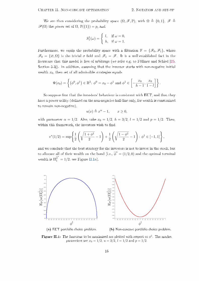
We are then considering the probability space (Ω,F ,P), with Ω , 0, 1, F ,
P(Ω) the power set of Ω, P(1) = p, and
S11(ω) =
l, if ω = 0,
h, if ω = 1.
Furthermore, we equip the probability space with a ltration F = F0,F1, whereF0 = ∅,Ω is the trivial σ-eld and F1 = F . It is a well-established fact in the
literature that this model is free of arbitrage (we refer e.g. to Föllmer and Schied [25,
Section 5.5]). In addition, assuming that the investor starts with non-negative initial
wealth x0, then set of all admissible strategies equals
Ψ(x0) =
(φ0, φ1
)∈ R2: φ0 = x0 − φ1 and φ1 ∈
[− x0
h− 1,x0
1− l
].
So suppose rst that the investors' behaviour is consistent with EUT, and that they
have a power utility (dened on the non-negative half-line only, for wealth is constrained
to remain non-negative),
u(x) , xα − 1, x ≥ 0,
with parameter α = 1/2. Also, take x0 = 1/2, h = 3/2, l = 1/2 and p = 1/2. Then,
within this framework, the investors wish to nd
v∗(1/2) = sup
1
2
(√1 + φ1
2− 1
)+
1
2
(√1− φ1
2− 1
): φ1 ∈ [−1, 1]
,
and we conclude that the best strategy for the investors is not to invest in the stock, but
to allocate all of their wealth on the bond (i.e., φ∗
= (1/2, 0) and the optimal terminal
wealth is Πφ∗
1 = 1/2, see Figure II.1a).
(a) EUT portfolio choice problem. (b) Non-concave portfolio choice problem.
Figure II.1: The functions to be maximised are plotted with respect to φ1. The marketparameters are x0 = 1/2, u = 3/2, l = 1/2 and p = 1/2.
16

Chapter II. Non-concave optimisation 3. One-step case
Next, let us suppose instead that the investors have the following non-concave utility
function,
u(x) ,
(x2 − 1
)/4, if x ∈ [0, 1] ,
x1/2 − 1, if x > 1.
so the function to be maximised over φ1 ∈ [−1, 1] is now
EP
[u
(1
2+ φ1
(S1
1 − 1))]
=1
8
[(1 + φ1
2
)2
− 1
]+
1
8
[(1− φ1
2
)2
− 1
].
It can be easily checked that, in this case, there exist two optimal portfolios: one that
consists of borrowing money to buy one share of the stock (which has terminal wealth
(−1) + 1/2 = −1/2 if the stock price goes down and (−1) + 3/2 = 1/2 when the stock
price goes up); the other one which involves short-selling one stock to invest in the bond
(with terminal wealth 1− 1/2 = 1/2 if the stock price goes down and 1− 3/2 = −1/2 if
the stock performs well). Hence, not only did the optimal investment strategy change,
but also it is no longer unique (it can be noted from Figure II.1b that the functional
to be maximised is not globally concave any more). It is also worth pointing out that
the optimal portfolio of EUT actually became the least attractive of all admissible
portfolios.
Hence, this very simple example provides an important motivation for the study
of the optimal portfolio problem for investors with a non-concave utility, since the
conclusions may be completely dierent, perhaps even opposite, to those of EUT.
3 Optimal strategy in the one-step case
In this section, we consider an F -measurable function Y : Ω → Rd, and a σ-algebra
G ⊆ F containing all P-null sets of F . This setting will be applied in the next section
with G = Ft−1 and Y = ∆St, for every xed t ∈ 1, . . . , T.Keeping in line with the notation of the previous section, we denote by Ξd the family
of all G -measurable functions ξ : Ω→ Rd.We shall also impose the following throughout, which can be regarded as absence of
arbitrage at each single-time period (cf. Assumption II.2.9).
Assumption II.3.1. For every ξ ∈ Ξd, if 〈ξ, Y 〉Rd ≥ 0 a.s., then 〈ξ, Y 〉Rd = 0 a.s..
Moreover, let PY |G : B(Rd)× Ω → [0, 1] be the unique (up to a set of measure
zero) regular conditional distribution for Y given G (its existence and uniqueness being
ensured for example by Theorem 10.2.2 in Dudley [22]). We know, by denition of
regular conditional distribution, that there exists some set Ω ∈ G , with P(Ωc)
= 0,
such that, for any ω ∈ Ω, the function
PY |G(·, ω) : B(Rd)→ [0, 1]
E 7→ PY |G(E,ω)
17
Chapter II. Non-concave optimisation 3. One-step case
is a probability measure on(Rd,B
(Rd)). Now, for each ω ∈ Ω, let supp
(PY |G(·, ω)
)represent the support of PY |G(·, ω) (which exists and is non-empty), and letD(ω) denote
the ane hull of supp(PY |G(·, ω)
), that is, D(ω) , aff
(supp
(PY |G(·, ω)
)). On the other
hand, when ω 6∈ Ω, simply consider D(ω) , Rd. Then obviously each D(ω) is an ane
subspace of Rd. We note further that, for every ω outside Ω, D(ω) is actually a linear
subspace. It is not dicult to check the following (the proof being identical to that of
Proposition II.2.10).
Proposition II.3.2. Under Assumption II.3.1, there exists a subset Ω of Ω, satisfying
P(
Ω \ Ω)
= 0, and such that D(ω) is actually a vector (or linear) subspace of Rd, for
all ω ∈ Ω.
Remark II.3.3. Note that the hypothesis that G contains all P-null subsets of Ω implies
in particular that Ω = Ω ∩(
Ω \ Ω)c∈ G . We further remark that P
(Ωc)
= 0. 3
In addition, for every G -measurable random variable H : Ω → R satisfying H ≥ 0
a.s., dene the set
Ξd(H) ,ξ ∈ Ξd: 〈ξ, Y 〉Rd ≥ −H a.s.
.
Then in the particular case where H = x a.s., for some x ∈ [0,+∞) , we have
Ξd(x) ,ξ ∈ Ξd: 〈ξ, Y 〉Rd ≥ −x a.s.
.
Finally, let Ξd denote the family of all functions ξ ∈ Ξd such that ξ(ω) ∈ D(ω) for
P-a.e. ω ∈ Ω.
Remark II.3.4. It is trivial to see that Ξd is non-empty. In fact, let ξ0 : Ω→ Rd be thenull function, that is, ξ0(ω) , 0d for every ω ∈ Ω. Then we have by Proposition II.3.2
that, for every ω ∈ Ω, the ane space D(ω) is actually a vector space, and hence
ξ0(ω) = 0d ∈ D(ω). 3
Like in the preceding section (cf. Proposition II.2.11), we can obtain the following.
Proposition II.3.5. Under Assumption II.3.1, there exist two G -measurable random
variables β : Ω→ R and κ : Ω→ R such that β > 0 a.s., κ > 0 a.s. and
P(〈ξ, Y 〉Rd ≤ −β ‖ξ‖Rd |G ) ≥ κ a.s. on Ω ,ω ∈ Ω: D(ω) 6= 0d
, (II.3.1)
for all ξ ∈ Ξd.
Remark II.3.6. We know from Lemma II.5.6 that Ω ∈ G . 3
The next result essentially says that any portfolio can be replaced with its orthogonal
projection11 on D without altering its value (except possibly on a null set).
11Given a linear subspace D of the Euclidean space Rn, the orthogonal projection on D is thelinear map prD : Rn → D where, for every x ∈ Rn, prD(x) is the (unique) vector in D such thatx− prD(x) ∈ D⊥ ,
y ∈ Rn: 〈x, y〉Rn = 0, ∀x ∈ D
.
18

Chapter II. Non-concave optimisation 3. One-step case
Proposition II.3.7. Let x ≥ 0 and ξ ∈ Ξd(x) be arbitrary, but xed. Under Assump-
tion II.3.1, if ξ : Ω→ Rd is the function dened by
ξ(ω) ,
prD(ω)(ξ(ω)) , if ω ∈ Ω,
ξ(ω) , otherwise,(II.3.2)
where prM : Rd → M is the orthogonal projection onto the subspace M of Rd, then ξbelongs to Ξd(x) and
x+⟨ξ, Y
⟩Rd
= x+ 〈ξ, Y 〉Rd a.s.. (II.3.3)
Proof. See Section II.5, page 31.
Now let V : [0,+∞) × Ω→ R be a function verifying the properties below.
Assumption II.3.8. The function V satises the following,
(i) for any xed x ∈ [0,+∞) , the function V (x, ·) : Ω→ R is measurable with respect
to F ,
(ii) for P-a.e. ω ∈ Ω, the function V (·, ω) : [0,+∞) → R is continuous on (0,+∞),
right-continuous at 0, and increasing on [0,+∞) , with V (1, ω) ≥ 0.
Remark II.3.9. We observe that, for every x ≥ 0 and for every ξ ∈ Ξd(x), the function
mapping each ω in Ω to V (x+ 〈ξ(ω) , Y (ω)〉Rd , ω) is well-dened, except possibly on
a set of P-measure zero. From this time forth, any function on Ω which is dened for
P-a.e. ω is considered to be well-dened. 3
We shall also need the following integrability conditions.
Assumption II.3.10. For every x ∈ [0,+∞) ,12
ess supξ∈Ξd(x)
EP[V +(x+ 〈ξ(·) , Y (·)〉Rd , ·)
∣∣G ] < +∞ a.s.. (II.3.4)
Remark II.3.11. It is obvious that Assumption II.3.10 implies that, for all x ≥ 0,
ess supξ∈Ξd(x)
EP [V (x+ 〈ξ(·) , Y (·)〉Rd , ·)|G ] < +∞ a.s.. (II.3.5)
3
Assumption II.3.12. The conditional expectation, with respect to G , of the function
V −(0, ·) : Ω→ [0,+∞) is nite a.s., i.e.,
EP[V −(0, ·)
∣∣G ] < +∞ a.s.. (II.3.6)
Finally, we impose the following growth condition on V .
12In order to make the notation less heavy, given any function f : X → R, we shall write henceforthf±(x) , [f(x)]± for all x ∈ X.
19
Chapter II. Non-concave optimisation 3. One-step case
Assumption II.3.13. There exist constants C > 0 and γ > 0 such that
Pω ∈ Ω: V +(λx, ω) ≤ λγV +(x, ω) + Cλγ, for all λ ≥ 1 and for all x ≥ 0
= 1.
(II.3.7)
Next, we proceed with two technical lemmata. The rst one essentially states that
any admissible portfolio can be replaced with its projection on D without changing the
desirability of the portfolio, whilst the second one shows that the set of all admissible
strategies in D is bounded.
Lemma II.3.14. Fix an arbitrary x ≥ 0. Then, under Assumption II.3.1, for every
ξ ∈ Ξd(x), we have
EP[V (x+ 〈ξ(·) , Y (·)〉Rd , ·)|G ] = EP
[V(x+
⟨ξ(·) , Y (·)
⟩Rd, ·)∣∣∣G ] a.s., (II.3.8)
where ξ is the projection given by (II.3.2).
Proof. See Section II.5, page 31.
Lemma II.3.15. Suppose that Assumption II.3.1 is in force. Given any x0 ≥ 0, there
exists a G -measurable, real-valued random variable Kx0 such that Kx0 > x0 a.s., and
for all x ∈ [0, x0] and all ξ ∈ Ξd(x) with ξ(ω) ∈ D(ω) for P-a.e. ω in Ω,
‖ξ‖Rd ≤ Kx0 a.s.. (II.3.9)
Proof. This is Lemma 2.1 in Rásonyi and Stettner [51]. For a proof, see Section II.5,
page 32.
As for the next lemma, it will allow us to apply certain convergence results for the
conditional expectation later on, namely the reverse Fatou lemma.
Lemma II.3.16. Suppose Assumptions II.3.1, II.3.8, II.3.10 and II.3.13 are in force.
Given any x ≥ 0, there is a non-negative random variable Lx : Ω → R such that
E[Lx|G ] < +∞ a.s. and, for every ξ ∈ Ξd(x) with ξ(ω) ∈ D(ω) for P-a.e. ω ∈ Ω, the
inequality
V +(x+ 〈ξ(·) , Y (·)〉Rd , ·) ≤ Lx (II.3.10)
holds almost surely.
Proof. This is Lemma 2.3 in Rásonyi and Stettner [51], and its proof is reproduced in
Section II.5, page 33.
Furthermore, we establish the existence of a regular version of the conditional ex-
pectation.
Lemma II.3.17. Let x0 ∈ [0,+∞) be xed, and let Assumptions II.3.8 and II.3.10 be
in force. For every ξ ∈ Ξd(x0), there exists a function Gξ : [x0,+∞) × Ω → R such
that
20
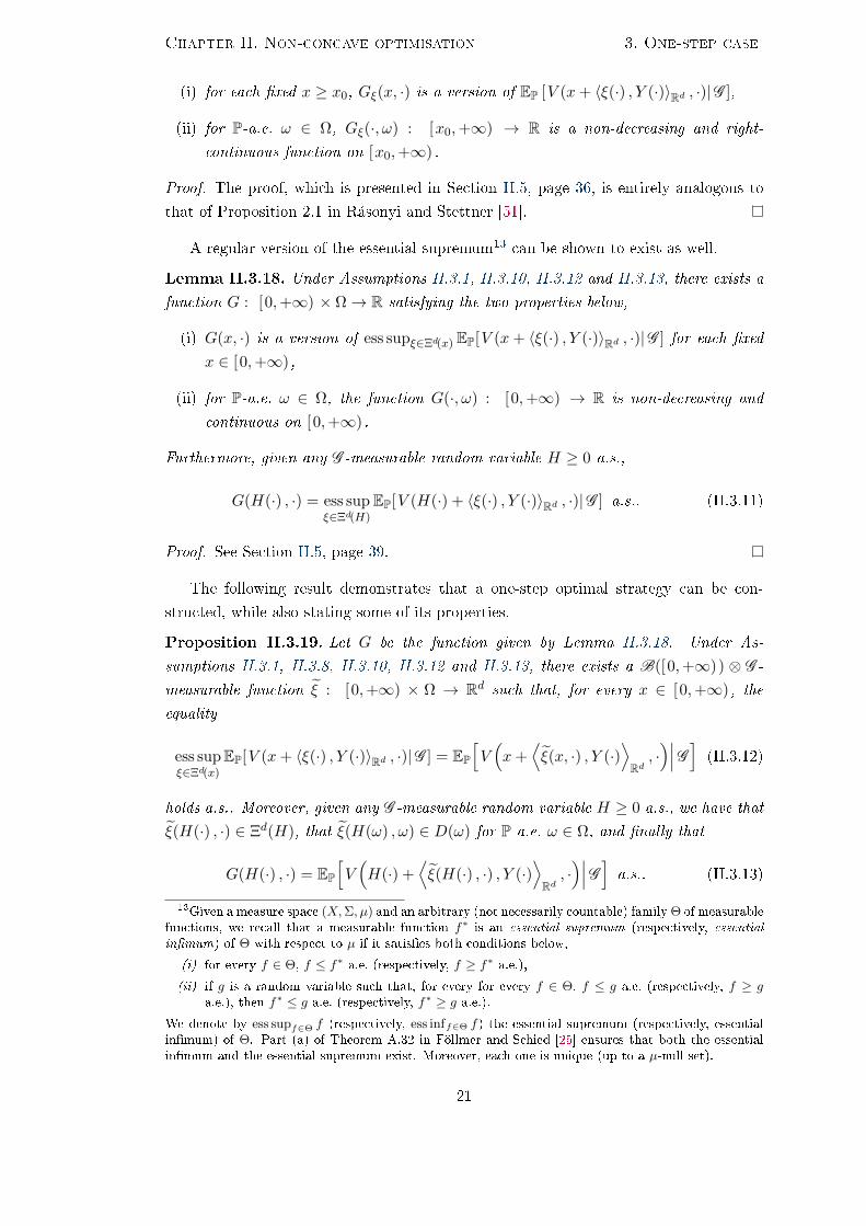
Chapter II. Non-concave optimisation 3. One-step case
(i) for each xed x ≥ x0, Gξ(x, ·) is a version of EP [V (x+ 〈ξ(·) , Y (·)〉Rd , ·)|G ],
(ii) for P-a.e. ω ∈ Ω, Gξ(·, ω) : [x0,+∞) → R is a non-decreasing and right-
continuous function on [x0,+∞) .
Proof. The proof, which is presented in Section II.5, page 36, is entirely analogous to
that of Proposition 2.1 in Rásonyi and Stettner [51].
A regular version of the essential supremum13 can be shown to exist as well.
Lemma II.3.18. Under Assumptions II.3.1, II.3.10, II.3.12 and II.3.13, there exists a
function G : [0,+∞) × Ω→ R satisfying the two properties below,
(i) G(x, ·) is a version of ess supξ∈Ξd(x) EP[V (x+ 〈ξ(·) , Y (·)〉Rd , ·)|G ] for each xed
x ∈ [0,+∞) ,
(ii) for P-a.e. ω ∈ Ω, the function G(·, ω) : [0,+∞) → R is non-decreasing and
continuous on [0,+∞) .
Furthermore, given any G -measurable random variable H ≥ 0 a.s.,
G(H(·) , ·) = ess supξ∈Ξd(H)
EP[V (H(·) + 〈ξ(·) , Y (·)〉Rd , ·)|G ] a.s.. (II.3.11)
Proof. See Section II.5, page 39.
The following result demonstrates that a one-step optimal strategy can be con-
structed, while also stating some of its properties.
Proposition II.3.19. Let G be the function given by Lemma II.3.18. Under As-
sumptions II.3.1, II.3.8, II.3.10, II.3.12 and II.3.13, there exists a B([0,+∞)) ⊗ G -
measurable function ξ : [0,+∞) × Ω → Rd such that, for every x ∈ [0,+∞) , the
equality
ess supξ∈Ξd(x)
EP[V (x+ 〈ξ(·) , Y (·)〉Rd , ·)|G ] = EP
[V(x+
⟨ξ(x, ·) , Y (·)
⟩Rd, ·)∣∣∣G ] (II.3.12)
holds a.s.. Moreover, given any G -measurable random variable H ≥ 0 a.s., we have that
ξ(H(·) , ·) ∈ Ξd(H), that ξ(H(ω) , ω) ∈ D(ω) for P-a.e. ω ∈ Ω, and nally that
G(H(·) , ·) = EP
[V(H(·) +
⟨ξ(H(·) , ·) , Y (·)
⟩Rd, ·)∣∣∣G ] a.s.. (II.3.13)
13Given a measure space (X,Σ, µ) and an arbitrary (not necessarily countable) family Θ of measurablefunctions, we recall that a measurable function f∗ is an essential supremum (respectively, essentialinmum) of Θ with respect to µ if it satises both conditions below,
(i) for every f ∈ Θ, f ≤ f∗ a.e. (respectively, f ≥ f∗ a.e.),(ii) if g is a random variable such that, for every for every f ∈ Θ, f ≤ g a.e. (respectively, f ≥ g
a.e.), then f∗ ≤ g a.e. (respectively, f∗ ≥ g a.e.).
We denote by ess supf∈Θ f (respectively, ess inff∈Θ f) the essential supremum (respectively, essentialinmum) of Θ. Part (a) of Theorem A.32 in Föllmer and Schied [25] ensures that both the essentialinmum and the essential supremum exist. Moreover, each one is unique (up to a µ-null set).
21
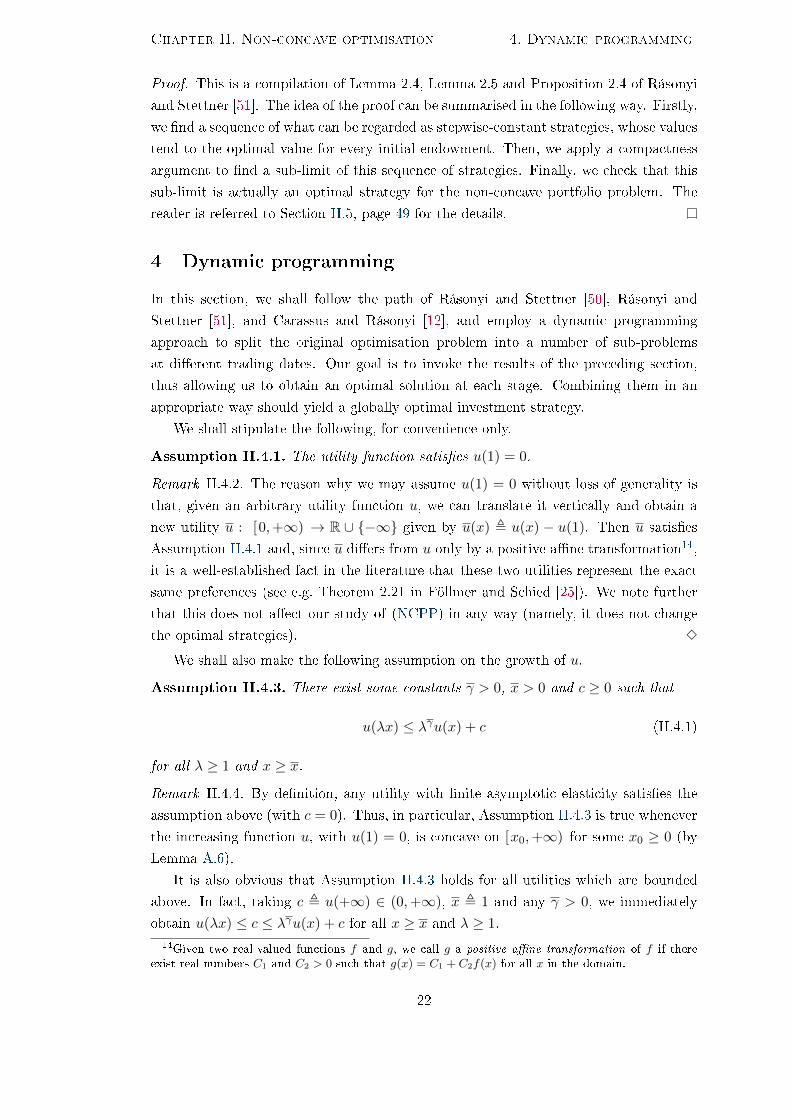
Chapter II. Non-concave optimisation 4. Dynamic programming
Proof. This is a compilation of Lemma 2.4, Lemma 2.5 and Proposition 2.4 of Rásonyi
and Stettner [51]. The idea of the proof can be summarised in the following way. Firstly,
we nd a sequence of what can be regarded as stepwise-constant strategies, whose values
tend to the optimal value for every initial endowment. Then, we apply a compactness
argument to nd a sub-limit of this sequence of strategies. Finally, we check that this
sub-limit is actually an optimal strategy for the non-concave portfolio problem. The
reader is referred to Section II.5, page 49 for the details.
4 Dynamic programming
In this section, we shall follow the path of Rásonyi and Stettner [50], Rásonyi and
Stettner [51], and Carassus and Rásonyi [12], and employ a dynamic programming
approach to split the original optimisation problem into a number of sub-problems
at dierent trading dates. Our goal is to invoke the results of the preceding section,
thus allowing us to obtain an optimal solution at each stage. Combining them in an
appropriate way should yield a globally optimal investment strategy.
We shall stipulate the following, for convenience only.
Assumption II.4.1. The utility function satises u(1) = 0.
Remark II.4.2. The reason why we may assume u(1) = 0 without loss of generality is
that, given an arbitrary utility function u, we can translate it vertically and obtain a
new utility u : [0,+∞) → R ∪ −∞ given by u(x) , u(x) − u(1). Then u satises
Assumption II.4.1 and, since u diers from u only by a positive ane transformation14,
it is a well-established fact in the literature that these two utilities represent the exact
same preferences (see e.g. Theorem 2.21 in Föllmer and Schied [25]). We note further
that this does not aect our study of (NCPP) in any way (namely, it does not change
the optimal strategies). 3
We shall also make the following assumption on the growth of u.
Assumption II.4.3. There exist some constants γ > 0, x > 0 and c ≥ 0 such that
u(λx) ≤ λγu(x) + c (II.4.1)
for all λ ≥ 1 and x ≥ x.
Remark II.4.4. By denition, any utility with nite asymptotic elasticity satises the
assumption above (with c = 0). Thus, in particular, Assumption II.4.3 is true whenever
the increasing function u, with u(1) = 0, is concave on [x0,+∞) for some x0 ≥ 0 (by
Lemma A.6).
It is also obvious that Assumption II.4.3 holds for all utilities which are bounded
above. In fact, taking c , u(+∞) ∈ (0,+∞), x , 1 and any γ > 0, we immediately
obtain u(λx) ≤ c ≤ λγu(x) + c for all x ≥ x and λ ≥ 1.14Given two real-valued functions f and g, we call g a positive ane transformation of f if there
exist real numbers C1 and C2 > 0 such that g(x) = C1 + C2f(x) for all x in the domain.
22
Chapter II. Non-concave optimisation 4. Dynamic programming
Since there are bounded utilities with innite AE (see Example A.13), having nite
asymptotic elasticity is a sucient, albeit not necessary, condition for a function to
verify Assumption II.4.3.
Finally, we remark that Assumption II.4.3 does not imply that u has strictly linear
growth (see e.g. Example II.2.15(viii)). 3
We may now deduce the following auxiliary result, which provides an estimate for
all x ≥ 0, and not only for x ≥ x.
Lemma II.4.5. Under Assumptions II.4.1 and II.4.3, there is some C ∈ (0,+∞) such
that, for all λ ≥ 1 and all x ≥ 0,
u+(λx) ≤ λγu+(x) + Cλγ . (II.4.2)
Proof. See Section II.5, page 59.
Hence, the next result, which is the main one of the present chapter, says that the
problem (NCPP) admits an optimal strategy under certain conditions (namely, that the
optimisation problem is well-posed, i.e., its supremum is nite).
Theorem II.4.6. Let Assumptions II.2.9 and II.2.16 and Assumptions II.4.1 and II.4.3
hold true. Assume further that, for every x0 ∈ [0,+∞) ,
supφ∈Ψ(x0)
EP
[u+(
ΠφT
)]< +∞. (II.4.3)
Then, for each x0 ∈ [0,+∞) , there exists a strategy φ∗
= φ∗(x0) ∈ A (x0) satisfying
EP
[u(
Πφ∗
T
)]= v∗(x0) . (II.4.4)
Proof. We give here a brief description of the proof, in which a dynamic programming
technique is applied, as already mentioned above. In order to be able to use the results of
the one-step case and thus get an optimal solution at each time step, we must recursively
conrm that all of the required assumptions are fullled. Once this is accomplished, we
paste together the aforementioned solutions to obtain an investment strategy, which we
then show to be an optimal one for (NCPP). The details can be found in Section II.5,
page 59.
Remark II.4.7. (i) The case where x0 = 0 is actually trivial. In fact, it is an obvious
consequence of the no-arbitrage Assumption II.2.9 that, for every φ ∈ Ψ(0), we
have ΠφT = 0 a.s., and so EP
[u+(
ΠφT
)]= u+(0) = 0, because u(0) ≤ u(1) = 0
(recall the monotonicity of u and Assumption II.4.1). Moreover, EP
[u(
ΠφT
)]=
u(0), hence v∗(0) = u(0) and thus all strategies are optimal (or equivalently, the
investor is indierent amongst all admissible strategies).
23
Chapter II. Non-concave optimisation 5. Proofs and auxiliary results
(ii) Note that (II.4.3) implies in particular that the expectation EP
[u(
ΠφT
)]is well-
dened (possibly −∞) for every φ ∈ Ψ(x0), hence all admissible strategies are
feasible for (NCPP), i.e., A (x0) = Ψ(x0). 3
As a very simple yet important example to which the preceding theorem clearly
applies, we mention the case of u bounded above and satisfying Assumption II.2.16 and
Assumption II.4.1. Another relevant example is given by the following.
Theorem II.4.8. Let Assumptions II.2.9 and II.2.16 and Assumptions II.4.1 and II.4.3
hold true. Assume further that ‖∆St‖Rd , 1/βt ∈ W for every t ∈ 1, . . . , T, where eachβt is the random variable given by Proposition II.2.11 and
W ,Y ∈ Ξ1
T : EP[|Y |p] < +∞ for all p > 0. (II.4.5)
Then, for every x0 ∈ [0,+∞) , condition (II.4.3) is satised and there exists an optimal
strategy φ∗
= φ∗(x0) ∈ A (x0).
Proof. See Section II.5, page 65.
5 Proofs and auxiliary results
5.1 Auxiliary results
Except where explicitly stated otherwise, assume everything is as in Section II.3.
The following elementary inequality will be used several times, not only in Chap-
ter II, but also in Chapter III.
Lemma II.5.1. Given any s > 0, the inequality
|x+ y|s ≤ C (|x|s + |y|s) (II.5.1)
holds for every x, y ∈ R, with C , 1 ∨ 2s−1 > 0.
Proposition II.5.2. Let the multi-function15 S : Ω⇒ Rd be as given below,
S (ω) ,
supp
(PY |G(·, ω)
), if ω ∈ Ω,
Rd, otherwise.(II.5.2)
Then S is measurable and closed-valued, with dom S = Ω.
Proof. That S is a closed-valued multi-function is a trivial consequence of the denition
of support of a measure. Moreover, given that PY |G(Rd, ω
)= 1 for every ω ∈ Ω, it
15Given a measurable space (X,Σ), we recall that S : X ⇒ Rn is a multi-function (or a set-valuedmapping) fromX to the Euclidean space Rn if every x ∈ X is associated with exactly one subset S (x) ofRn. Moreover, we call a multi-function S closed-valued if, for all x ∈ X, the set S (x) is closed in Rn. Inaddition, the inverse image under S of a set U ⊆ Rn is given by S−1(U) , x ∈ X: S (x) ∩ U 6= ∅,and so the domain of S is taken to be the inverse image of Rn, that is, dom S , x ∈ X: S (x) 6= ∅.Also, the graph of S is the set gph S , (x, y) ∈ X × Rn: x ∈ dom S and y ∈ S (x). Finally, S ismeasurable if, for every open set O ⊆ Rn, S−1(O) ∈ Σ.
24
Chapter II. Non-concave optimisation 5. Proofs and auxiliary results
follows immediately that dom S = Ω. Besides, using the density16 of the rationals, it
is easy to check that17
gph S =
⋂ρ∈Q+
⋃q∈Qd
[([PY |G
(Bd(q, ρ) , ·
)−1((0, 1])
]∩ Ω
)× Bd(q, ρ)
]∪ [Ωc × Rd].
But, for every q ∈ Qd and ρ ∈ Q+, PY |G(Bd(q, ρ) , ·
)is a G -measurable random
variable, consequently gph S ∈ G ⊗ B(Rd), which combined with the completeness
of (Ω,G ,P) concludes the proof (we refer to Theorem 14.8 in Rockafellar and Wets
[53]).
Corollary II.5.3. The multi-function D : Ω ⇒ Rd dened by D(ω) , aff(S (ω)),
where S : Ω ⇒ Rd is the mapping of Proposition II.5.2, is also closed-valued and
measurable, with dom D = Ω. In particular, this implies that
D ,
(ω, y) ∈ Ω× Rd: y ∈ D(ω)∈ G ⊗B
(Rd). (II.5.3)
Proof. Measurability follows immediately from Proposition II.5.2 and Exercise 14.12
in Rockafellar and Wets [53], whereas closed-valuedness is a direct consequence of Ex-
ercise 2.11 in Rockafellar and Wets [53]. Finally, we notice that D = gph D , so the
measurability of the set D follows from Theorem 14.8 in Rockafellar and Wets [53] and
the fact that D is closed-valued.
Proposition II.5.4. Suppose A is a G -random set18. Then ω ∈ Ω: (ω, Y (ω)) ∈ Abelongs to the σ-algebra F and
Pω ∈ Ω: (ω, Y (ω)) ∈ A =
∫ΩPY |G(Aω, ω) dP(ω) , (II.5.4)
where Aω ∈ B(Rd)is the section19 of A determined by ω in Ω.
Proof. Let us consider any A ∈ G ⊗B(Rd). We shall begin by showing that the set
ω ∈ Ω: (ω, Y (ω)) ∈ A is in F . Indeed, setting f(ω) , 11A(ω, Y (ω)) for every ω ∈ Ω,
it is clear that f is F -measurable, therefore ω ∈ Ω: (ω, Y (ω)) ∈ A = f−1(1) ∈ F .
Next, we turn to the proof of (II.5.4). In order to do so, let us start by supposing
that A = G × E, with G ∈ G and E ∈ B(Rd), is a measurable rectangle. Then the
16A subset D of a topological space (S, τ) is dense in S if cl(D) = S, where the topological closurecl(D) of D is the smallest closed set in S containing D.
17Here, Bn(x0, r) ,x ∈ Rn: ‖x− x0‖Rn < r
denotes the open ball of centre x0 ∈ Rn and radius
r > 0 in the Euclidean space Rn.18Given a measurable space (X,Σ) and n ∈ N, we say that a subset E of X × Rn is a Σ-random set
if it belongs to the product σ-algebra Σ⊗B(Rn).19Let X and Y be two non-empty sets, and consider a subset E of X × Y . For every x ∈ X (re-
spectively, y ∈ Y ), the x-section (respectively, y-section) of E is dened by Ex , y ∈ Y : (x, y) ∈ E(respectively, Ey , x ∈ X: (x, y) ∈ E).
25

Chapter II. Non-concave optimisation 5. Proofs and auxiliary results
following holds a.s.,
P ω ∈ Ω: (ω, Y (ω)) ∈ A|G = EP[11G∩[Y −1(E)]
∣∣G ] = 11G PY |G(E, ·) ,
where the second inequality follows from the fact that G ∈ G and from the denition
of regular conditional distribution.
Moreover, it is trivial to see that the section of A determined by every xed ω ∈ Ω
equals
Aω =
E, if ω ∈ G,∅, otherwise,
hence PY |G(Aω, ω) = 11G(ω)PY |G(E,ω) for any ω ∈ Ω.
Combining the above yields P ω ∈ Ω: (ω, Y (ω)) ∈ A|G (ω) = PY |G(Aω, ω) for P-a.e. ω ∈ Ω, so taking expectations on both sides of the equality allows us to conclude
that (II.5.4) is true for all measurable rectangles of Ω× Rd.The validity of the result for an arbitrary A ∈ G ⊗B
(Rd)can now be derived in
the classic way, using Dynkin's π-λ theorem (see, e.g., Lemma 4.11 in Aliprantis and
Border [1]).
Corollary II.5.5. The set ω ∈ Ω: Y (ω) ∈ D(ω) belongs to the σ-algebra F and has
P-full measure.
Lemma II.5.6. Under Assumption II.3.1, the set Ω ,ω ∈ Ω: D(ω) 6= 0d
belongs
to the σ-algebra G . Moreover, P(
Ω)
= 0 if and only if Y = 0d a.s..
Proof. Given that, for every ω ∈ Ω, the linear space D(ω) contains the vector 0d
(see Proposition II.3.2), it is clear that Ω =ω ∈ Ω: D(ω) ∩
(Rd \ 0d
)6= ∅
= Ω ∩
D−1(Rd \ 0d
)∈ G , where D is the measurable multi-function of Corollary II.5.3.
Let us now prove the equivalence. We can use Proposition II.5.4 to rst obtain
the equality Pω ∈ Ω: Y (ω) 6= 0d =∫
Ω PY |G(Rd \ 0d , ω
)dP(ω), therefore Y = 0d
a.s. if and only if PY |G(Rd \ 0d , ·
)= 0 a.s.. But if the latter holds, then it follows
from the denition of support that supp(PY |G(·, ω)
)⊆ 0d for P-a.e. ω ∈ Ω, which in
turn implies that P(
Ω)
= 0. Reciprocally, if P(
Ω)
= 0 is true, then for P-a.e. ω ∈ Ω,
∅ 6= supp(PY |G(·, ω)
)⊆ D(ω) = 0d, hence by the denition of support we have
PY |G(Rd \ 0d , ω
)= PY |G
(supp
(PY |G(·, ω)
)c, ω)
= 0.
Lemma II.5.7. Let Θ be a collection (not necessarily countable) of F -measurable ran-
dom variables. If for every pair f, g ∈ Θ and for every A ∈ F we have f11A+g11Ac ∈ Θ,
then the family EP[f |G ] ; f ∈ Θ is directed both upwards and downwards20.
20For every x, y ∈ R, let x ∨ y , maxx, y and x ∧ y , minx, y. Then, given a measure space(X,Σ, µ), we say that an arbitrary family Θ (not necessarily countable) of measurable functions isdirected upwards (respectively, directed downwards) if, for every f1, f2 ∈ Θ, there exists some g ∈ Θsuch that g ≥ f1 ∨ f2 (respectively, g ≤ f1 ∧ f2) µ-a.e..
26
Chapter II. Non-concave optimisation 5. Proofs and auxiliary results
Proof. For every xed pair of random variables f and g in Θ, take hu : Ω → R and
hd : Ω→ R to be the F -measurable random variables respectively given by
hu(ω) , f(ω) 11EP[f |G ]≥EP[g |G ](ω) + g(ω) 11EP[f |G ]<EP[g |G ](ω) , and
hd(ω) , f(ω) 11EP[f |G ]<EP[g |G ](ω) + g(ω) 11EP[f |G ]≥EP[g |G ](ω) .
Lemma II.5.8. Let x ≥ 0 be xed. Under Assumption II.3.1, there exists a G -random
set M(x) such that, for P-a.e. ω ∈ Ω, the section M(x)ω of M(x) determined by ω is
non-empty, convex and compact21. Moreover, given any G -measurable random variable
ξ : Ω→ Rd, the following two statements are equivalent,
(i) ξ ∈ Ξd(x) and ξ(ω) ∈ D(ω) for P-a.e. ω ∈ Ω,
(ii) ξ(ω) ∈M(x)ω for P-a.e. ω ∈ Ω.
Proof. This is Proposition 4.2 in Rásonyi and Stettner [51], we include its proof here
for completeness.
Let us x an arbitrary x ∈ [0,+∞) . We know by the proof of Proposition II.5.2
that the graph of the multi-function S : Ω ⇒ Rd given by (II.5.2) is in G ⊗B(Rd),
hence S admits a Castaing representation22 ςn; n ∈ N (this follows from Castaing
and Valadier [16, Theorem III.22]). Now we dene the set
M(x) , D ∩
(⋂n∈N
f−1n ([−x,+∞))
),
whereD is given by (II.5.3) and fn : Ω×Rd → R is the(G ⊗B
(Rd),B(R)
)-measurable
function dened by fn(ω, y) , 〈y, ςn(ω)〉Rd , for every n ∈ N.Clearly, M(x) belongs to G ⊗B
(Rd). Furthermore, the section ofM(x) determined
by each ω ∈ Ω equals
M(x)ω = D(ω) ∩
(⋂n∈N
(〈·, ςn(ω)〉Rd)−1([−x,+∞))
),
which, being the countable intersection of convex and closed subsets of Rd (we recall thatevery ane space is closed and convex, and that convexity and closedness are preserved
under inverse images of continuous functions), is itself convex and closed. Also, it is
obvious that M(x)ω 6= ∅ for all ω ∈ Ω. In fact, if ω ∈ Ω, it is trivial that 0d ∈ M(x)ω(we invoke Proposition II.3.2), whereas for ω 6∈ Ω, either 0d ∈ D(ω) or there must
be at least one n ∈ N such that ςn(ω) 6= 0d, hence 0d ∈ M(x)ω or ςn(ω) ∈ M(x)ω,
respectively.21Recall that a subset K of a topological space (S, τ) is compact if for every indexed (not necessarily
countable) family Oi∈I ; i ∈ I of open sets such that K ⊂⋃i∈I Oi, there is a nite subset J of I such
that K ⊂⋃j∈J Oj (that is, any open cover of Khas a nite subcover).
22We recall that a Castaing representation of a multi-function S : X ⇒ Rn is any countable familyσn; n ∈ N of measurable functions σn : dom S → Rn satisfying S (x) = cl(σn(x) ; n ∈ N) forevery x ∈ dom S .
27

Chapter II. Non-concave optimisation 5. Proofs and auxiliary results
We proceed with the proof that (i) holds if and only if (ii) is true. To show necessity,
consider any ξ ∈ Ξd(x) verifying ξ(ω) ∈ D(ω) for P-a.e. ω ∈ Ω. Then, setting A ,(ω, y) ∈ Ω× Rd: 〈ξ(ω) , y〉Rd < −x
∈ G ⊗B
(Rd), we obtain∫
ΩPY |G(Aω, ω) dP(ω) = Pω ∈ Ω: (ω, Y (ω)) ∈ A = 0,
where we use Proposition II.5.4 to deduce the rst equality. But this implies that
PY |G(A·, ·) = 0 a.s., and so, given that Aω =y ∈ Rd: 〈ξ(ω) , y〉Rd < −x
is an open
subset of Rd, we must have by denition of support of a measure that
supp(PY |G(·, ω)
)⊆ Acω =
y ∈ Rd: 〈ξ(ω) , Y (ω)〉Rd ≥ −x
for P-a.e. ω ∈ Ω. Thus, in particular, we get for P-a.e. ω ∈ Ω that
〈ξ(ω) , ςn(ω)〉Rd ≥ −x, ∀n ∈ N,
which establishes the desired implication. Next, we turn to the proof of suciency,
so consider any ξ ∈ Ξd, and suppose there exists some measurable set Ω1 ⊆ Ω, with
P(Ωc1) = 0, such that ξ(ω) ∈ M(x)ω for every ω ∈ Ω1. Then, in particular, we have
ξ(ω) ∈ D(ω) for P-a.e. ω ∈ Ω. On the other hand, it is easy to check that, for all
ω ∈ Ω1 ∩ Ω, the inclusion supp(PY |G(·, ω)
)⊆y ∈ Rd: x+ 〈ξ(ω) , y〉Rd ≥ 0
holds
true. Indeed, the result is trivial when ξ(ω) = 0d, thus let us assume instead that
‖ξ(ω)‖Rd 6= 0. Then, xing any y ∈ supp(PY |G(·, ω)
)and considering an arbitrary
ε > 0, we can nd some n ∈ N such that ‖y − ςn(ω)‖Rd < ε/ ‖ξ(ω)‖Rd , hence we can
use the Cauchy-Schwarz inequality to deduce
x+ 〈ξ(ω) , y〉Rd = x+ 〈ξ(ω) , ςn(ω)〉Rd + 〈ξ(ω) , y − ςn(ω)〉Rd≥ 0− ‖ξ(ω)‖Rd ‖y − ςn(ω)‖Rd > −ε,
and the arbitrarity of ε yields the claimed inclusion. Consequently, the monotonicity of
any measure along with the denition of support yield
1 = PY |G(
supp(PY |G(·, ω)
), ω)≤ PY |G
(y ∈ Rd: x+ 〈ξ(ω) , y〉Rd ≥ 0
, ω)
for P-a.e. ω ∈ Ω. As before, an obvious application of Proposition II.5.4 then gives the
intended result Px+ 〈ξ, Y 〉Rd ≥ 0 = 1.
Finally, we see that, for P-a.e. ω ∈ Ω, the section M(x)ω is a bounded set in Rd. Inorder to do so, we begin by noticing that the multi-function
Mx : Ω⇒ Rd
ω 7→M(x)ω ,
is non-empty and closed-valued. We remark further that gph Mx is measurable, hence
28

Chapter II. Non-concave optimisation 5. Proofs and auxiliary results
we can invoke the von Neumann-Aumann selection theorem (see e.g. Theorem III.22 in
Castaing and Valadier [16]) to obtain a Castaing representation µn; n ∈ N for Mx.
Therefore, we have µn(ω) ∈ M(x)ω for all ω ∈ Ω and for every n ∈ N, so by the
equivalence proved above, we conclude that each µn ∈ Ξd(x) and µn(ω) ∈ D(ω) for
P-a.e. ω ∈ Ω. Now x any ω in the P-full measure set⋂n∈N ‖µn‖Rd ≤ Kx, with Kx
the random variable found in Lemma II.3.15, and let y ∈M(x)ω be arbitrary. For each
ε > 0, there exists some µn satisfying ‖y − µn(ω)‖Rd < ε, hence the triangle inequality
yields ‖y‖Rd < Kx(ω) + ε. It now follows from the arbitrarity of ε that ‖y‖Rd ≤ Kx(ω)
for all y ∈M(x)ω, and we conclude the proof with the well-known result that a subset
of the Euclidean space Rd is compact if and only if it is closed and bounded.
Lemma II.5.9. Given any x ≥ 0, let M(x) be the set of Lemma II.5.8. Then, under
Assumption II.3.1, the sets
M(x) ,
(ω, y) ∈ Ω× Rd: y ∈ ri(M(x)ω), and (II.5.5)
Z(x) ,
(ω, y) ∈ Ω× Rd: y ∈ lin(M(x)ω), (II.5.6)
where ri(M(x)ω) and lin(M(x)ω) respectively denote the relative interior23 and the linear
span of the section M(x)ω, belong to the product σ-algebra G ⊗B(Rd).
Proof. This is the statement of Proposition 4.3 in Rásonyi and Stettner [51]. We provide
an alternative proof below.
Fix an arbitrary x ∈ [0,+∞) . In order to improve readability, we shall divide the
proof into two parts.
(i) First, it is straightforward to show that Z(x) is a G -random set. Indeed, let us de-
ne the multi-function Zx : Ω⇒ Rd by Zx(ω) , lin(M(x)ω). It then follows from
Lemma II.5.8 and Rockafellar and Wets [53, Theorem 14.8 and Exercise 14.12]
that Zx is measurable with dom Zx = Ω. In addition, since any linear space is an
ane space, we have that Zx is also closed-valued (we refer e.g. to Exercise 2.11
in Rockafellar and Wets [53]), thus Theorem 14.8 in Rockafellar and Wets [53]
gives Z(x) = gph Zx ∈ G ⊗B(Rd).
(ii) Secondly, we verify thatM(x) belongs to G ⊗B(Rd)as well. Using the denition
of relative interior and the density of Q+ in R+, it is immediate to check that
M(x) =⋃ρ∈Q+
(ω, y) ∈ Ω× Rd: Bd(y, ρ) ∩ aff(M(x)ω) ⊆M(x)ω
.
Next, combining Lemma II.5.8 with Rockafellar and Wets [53, Theorem 14.8 and
23For any set E ⊆ Rn, the relative interior of E, denoted by ri(E), is the interior of E relative to itsane hull, i.e., ri(E) , x ∈ Rn: Bn(x, r) ∩ aff(E) ⊆ E for some r > 0.
29

Chapter II. Non-concave optimisation 5. Proofs and auxiliary results
Exercise 14.12], as in the previous step, yields that the multi-function
Nx : Ω⇒ Rd
ω 7→ aff(M(x)ω) ,
is measurable and closed, so it admits a Castaing representation αn; n ∈ N(again, we use Theorem 14.8 in Rockafellar and Wets [53], and the von Neumann-
Aumann selection theorem). Thus, for every ρ ∈ Q+ and n ∈ N, let fρn : Ω ×Rd → 0, 1 and gn : Ω × Rd → 0, 1 be the G ⊗B
(Rd)-measurable functions
respectively given by
(ω, y) 7→ (αn(ω) , y) 7→ 11Eρ(αn(ω) , y)
with Eρ ,
(y, z) ∈ Rd × Rd: ‖y − z‖Rd ∈ [0, ρ)∈ B
(Rd)⊗B
(Rd), and
(ω, y) 7→ (ω, αn(ω)) 7→ 11M(x)(ω, αn(ω)) .
It is now obvious that not only does A ,⋃q∈Q+
⋂n∈N (gn − fρn)
−1([0,+∞)) be-
long to the product σ-algebra G ⊗B(Rd), but also it containsM(x). Conversely,
let (ω, y) ∈ Ω×Rd be such that, for some ρ ∈ Q+, we have (gn − fρn)(ω, y) ≥ 0 for
all n ∈ N. Taking % , ρ/2 ∈ Q+, let us x an arbitrary z ∈ Bd(y, %)∩aff(M(x)ω),
as well as an arbitrary ε > 0. Therefore, choosing τ in (0, 1 ∧ %/ε), it is possibleto nd some m ∈ N for which ‖z − αm(ω)‖Rd < τε. Consequently,
‖y − αm(ω)‖Rd ≤ ‖y − z‖Rd + ‖z − αm(ω)‖Rd < %+ τε < 2% = ρ
by the triangle inequality, and so 1 = 11Eρ(αm(ω) , y) ≤ 11M(x)(ω, αm(ω)), which
implies that αm(ω) ∈M(x)ω. But then, given that (1− τ) ε > 0, there must exist
some n ∈ N such that ‖αm(ω)− µn(ω)‖Rd < (1− τ) ε, where the Castaing repre-
sentation µn(ω) ; n ∈ N for Mx is the one obtained in the proof of Lemma II.5.8.
Combining all of the preceding results nally gives
‖z − µn(ω)‖Rd ≤ ‖z − αm(ω)‖Rd + ‖αm(ω)− µn(ω)‖Rd < τε+ (1− τ) ε = ε.
We then conclude that z ∈ M(x)ω, hence A ⊆ M(x), and the measurability of
the set M(x) is established.
5.2 Proofs of Section II.2
Proof of Proposition II.2.10. Fix t ∈ 1, . . . , T, and set Ωt ,ω ∈ Ωt: 0d ∈ Dt(ω)
.
We remark that any ane space containing the origin is actually a linear space, so it
suces to see that (i) and (ii) hold true.
The rst condition can be checked immediately. Indeed, since the multi-function
30
Chapter II. Non-concave optimisation 5. Proofs and auxiliary results
Dt : Ω⇒ Rd given by
Dt(ω) ,
Dt(ω) , if ω ∈ Ωt,
Rd, otherwise,
is closed-valued and measurable (see Corollary II.5.3), we can make use of Theorem 14.3
in Rockafellar and Wets [53] to conclude that Ωt = Ωt ∩D−1t (0d) ∈ Ft−1.
As for the argument to show (ii), it is essentially the same as that of the proof of
Theorem 3 in Jacod and Shiryaev [28].
5.3 Proofs of Section II.3
Proof of Proposition II.3.7. Let us begin by showing that ξ is in Ξd(x). We know, by
Corollary II.5.3, that the closed-valued mapping D given therein is measurable. Thus,
Theorem 14.8 in Rockafellar and Wets [53] and the von Neumann-Aumann theorem
ensure the existence of a countable sequence σnn∈N of G -measurable random variables
σn : Ω→ Rd such that, for every ω ∈ Ω, D(ω) = cl(σn(ω) ; n ∈ N).Next, let us consider the set E ,
[[Ω× Rd
]∩D ∩
(⋂n∈N h
−1n (0)
)]∪[Ωc × Rd
],
with hn : Ω×Rd → R the measurable function given by hn(ω, y) , 〈ξ(ω)− y, σn(ω)〉Rd .Then it is clear that E is a G -measurable random set. Moreover, for any xed ω ∈ Ω,
the section of E determined by ω is equal to
Eω =
ξ(ω)
, if ω ∈ Ω,
Rd, otherwise.
Hence, the multi-function E : Ω ⇒ Rd given by E (ω) , Eω (and whose graph equals
E) admits a measurable selector, that is, we can obtain a G -measurable random variable
f : Ω → Rd with f(ω) ∈ E (ω) for all ω ∈ Ω. But, since P(
Ωc)
= 0, this implies that
ξ = f a.s. and so ξ is a G -measurable random variable.
We now proceed to prove that the inequality x+⟨ξ, Y
⟩Rd≥ 0 holds a.s. and, as a
by-product, we shall deduce equation (II.3.3). For all ω ∈ Ω, we have that ξ(ω)− ξ(ω) ∈D(ω)⊥. Furthermore, we know by Corollary II.5.5 that B , ω ∈ Ω: Y (ω) ∈ D(ω) isin F and has full probability. Finally, given that ξ ∈ Ξd(x) by hypothesis, we can nd
a measurable set C ∈ F with P(Cc) = 0 and x + 〈ξ(ω) , Y (ω)〉Rd ≥ 0 for all ω ∈ C.Consequently, if we consider any ω ∈ Ω1 , Ω ∩B ∩ C, we obtain that
x+⟨ξ(ω) , Y (ω)
⟩Rd
= x+ 〈ξ(ω) , Y (ω)〉Rd ≥ 0,
where the equality is due to⟨ξ(ω)− ξ(ω) , Y (ω)
⟩Rd
= 0. The above equation combined
with P(Ωc1) = 0 then yields the intended results.
Proof of Lemma II.3.14. In order to check that equality (II.3.8) is true, let us start by
31
Chapter II. Non-concave optimisation 5. Proofs and auxiliary results
showing that the R-valued function given by
ω 7→ V (x+ 〈ξ(ω) , Y (ω)〉Rd , ω)
is F -measurable. In fact, let us dene the functions f : Ω→ R× Ω, g : R× Ω→ R2
and pr2 : R2 → R as follows, f(ω) , (x+ 〈ξ(ω) , Y (ω)〉Rd , ω), g(y, ω) , (y, V (y, ω)),
and pr2(y, z) , z. Clearly, f is (F ,B(R)⊗F )-measurable, because ξ and Y are
F -measurable, and the inner product and the sum in R2 are continuous functions.
Moreover, we have that pr2 is(B(R2),B(R)
)-measurable, by continuity. On the other
hand, is is trivial to check that V (x+ 〈ξ(ω) , Y (ω)〉Rd , ω) = (pr2 g f)(ω) for every
ω ∈ Ω, therefore we only need to check that g is(B(R)⊗F ,B
(R2))-measurable. In
order to do so, let O be an open subset of R2. Then O =⋃n∈NO
1n × O2
n, where Oin is
an open subset of R, for every i ∈ 1, 2 and n ∈ N. Furthermore, for every ω outside
some P-null set N , the function V (·, ω) is continuous. Therefore,
g−1(O) =
[R× (Ω \N)] ∩
⋃n∈N
[O1n × Ω
]∩
⋃ρ∈Q+
⋂q∈Q
(hnρ,q
)−1([0,+∞))
∪[g−1(O) ∩ [R×N ]
]∈ B(R)⊗F ,
where hnρ,q(y, ω) , 11Enρ,q(ω)− 11B(q,ρ)(y), Enρ,q , (V (q, ·))−1(Anρ) ∈ G (because V (q, ·) isG -measurable), and Anρ ,
⋂z /∈O2
n(|z − ·|)−1([ρ,+∞)) ∈ B(R) (because the intersection
of closed sets is still a closed set).
It follows from a completely identical argument that the function dened by
ω 7→ V(x+
⟨ξ(ω) , Y (ω)
⟩Rd, ω)
is F -measurable as well.
It then suces to note that V (x+ 〈ξ(·) , Y (·)〉Rd , ·) and V(x+
⟨ξ(·) , Y (·)
⟩Rd, ·)
are equal a.s., which is an immediate consequence of (II.3.3).
Proof of Lemma II.3.15. Fix x0 ≥ 0 and let β be the real-valued random variable given
by Proposition II.3.5. Then the function Kx0 : Ω→ R dened by
Kx0(ω) ,x0 + 1
β(ω)11β>0(ω) , ω ∈ Ω,
is clearly non-negative and G -measurable. Moreover, Kx0 > 0 a.s..
Next, let x ∈ [0, x0] be arbitrary, and consider any ξ ∈ Ξd(x) satisfying ξ(ω) ∈ D(ω)
for P-a.e. ω in Ω. Setting B , ω ∈ Ω: ‖ξ‖Rd > Kx0(ω), it can be easily checked that
B ∈ G and
x+ 〈ξ(ω) , Y (ω)〉Rd ≤ x− β(ω) ‖ξ(ω)‖Rd < x− β(ω)Kx0(ω) = x− (x0 + 1) < 0
for every ω ∈ B ∩ ω ∈ Ω: β(ω) > 0 ∩ ω ∈ Ω: 〈ξ(ω) , Y (ω)〉Rd ≤ −β(ω) ‖ξ(ω)‖Rd.
32

Chapter II. Non-concave optimisation 5. Proofs and auxiliary results
Therefore,
0 ≤ P(
Ω ∩B ∩ 〈ξ, Y 〉Rd ≤ −β ‖ξ‖Rd)≤ P(B ∩ 〈ξ, Y 〉Rd ≤ −β ‖ξ‖Rd)
= P(B ∩ β > 0 ∩ 〈ξ, Y 〉Rd ≤ −β ‖ξ‖Rd)
≤ Px+ 〈ξ, Y 〉Rd < 0 = 0,
where the rst and last equalities are due to β > 0 a.s. and ξ ∈ Ξd(x), respectively.
On the other hand, we know again by Proposition II.3.5 that
κ 11Ω∩B ≤ P
(Ω ∩B ∩ 〈ξ, Y 〉Rd ≤ −β ‖ξ‖Rd
∣∣∣G) a.s.,
so taking expectations on both sides and invoking the preceding equality, we obtain
EP[κ 11
Ω∩B]
= 0.
But, given that κ > 0 a.s., this implies that the set Ω∩B has probability zero, hence
P(B) = P(
Ω ∩B)
= P(ω ∈ Ω: D(ω) = 0d
∩B
)= P
(ω ∈ Ω: D(ω) = 0d
∩B ∩
ω ∈ Ω: ξ(ω) ∈ D(ω)
)= 0,
as ‖ξ(ω)‖Rd = 0 ≤ Kx0(ω) for all ω ∈ω ∈ Ω: D(ω) = 0d
∩ω ∈ Ω: ξ(ω) ∈ D(ω)
.
Proof of Lemma II.3.16. Fixing an arbitrary x ≥ 0, let us consider the G -random
set M(x) of admissible strategies in D, given by Lemma II.5.8. Then we know by
Lemma II.5.9 that its linear span Z(x) belongs to σ-algebra G ⊗B(Rn) as well.
Let us now organise the proof into four distinct parts.
(i) Firstly, it is not dicult to show that we can recursively choose G -measurable,
Rd-valued functions ζ1, . . . , ζd such that, for every ω ∈ Ω, ζ1(ω) , . . . , ζd(ω) is anorthogonal set24 of vectors spanning Z(x)ω (note that some, or even all, of them
may eventually be the null vector), and ‖ζi(ω)‖Rd ∈ 0, 1 for every i ∈ 1, . . . , d.
(ii) Next, we show that M(x)ω is contained in a simplex25, for P-a.e. ω ∈ Ω. Indeed,
it follows from the proof of Lemma II.5.8 and from Lemma II.3.15 that, for all ω
outside a P-null set N = N(x), M(x)ω is contained in the set
Px(ω) , Z(x)ω ∩y ∈ Rd: Ax(ω) y ≤ bx(ω)
,
with Ax and bx respectively the (2d)×d random matrix and the d×1 random vector
with coecients26 (Ax)ij , (−1)i(ζdi/2e
)jand (bx)j , Kx for all i ∈ 1, . . . , 2d
24Given a vector space V with an inner product 〈·, ·〉, we say that a set E ⊆ V is an orthogonal setif, for every x, y ∈ E with x 6= y, we have 〈x, y〉 = 0.
25A set S ⊆ Rn is called a simplex if it is the convex hull of a nite number of points, that is,S = conv(x1, . . . , xp) for some p ∈ N0 and x1, . . . , xp ∈ Rn.
26The ceiling function d·e : R → Z and the oor function b·c : R → Z are respectively given by
33

Chapter II. Non-concave optimisation 5. Proofs and auxiliary results
and j ∈ 1, . . . , d. It is also obvious that 0d ∈ Px(ω), so Px(ω) is non-empty.
Moreover, it can be easily checked that Px(ω) is closed and convex (recall that
the pre-image of a closed set under a continuous function is closed as well, that
every linear space is closed and convex, and nally that the intersection of closed
and convex sets is still closed and convex). It is also immediate to see that Px(ω)
is contained in Bd(0d,√dKx(ω)
), that is, Px(ω) is bounded.
As a consequence of the nite-dimensional version of the Krein-Milman theorem
(we refer e.g. to Barnikov [7, Theorem II.3.3]), we conclude that every Px(ω) is
the convex hull of the set of its extreme points27 (which is non-empty). Dening
the 2d random vectors
θi(ω) , Kx(ω)
d∑j=1
(ιi)j ζj(ω) ,
where ι1, . . . , ι2d = −1, 1d is the set of vectors in Rd whose components have
absolute value equal to 1, it is easy to verify that E(Px(ω)) = θ1(ω) , . . . , θ2d(ω).
(iii) Thirdly, Lemma II.5.9 tells us thatM(x) is also a G -random set, so we can apply
the von Neumann-Aumann theorem to obtain a G -measurable selector % : Ω→ Rd
of M(x). Next, for every i ∈
1, . . . , 2d, let us dene the set
Ei,(ω, λ) ∈ Ω× (0, 1) : (1− λ) %(ω)+λ θi(ω) ∈M(x)ω=(11M(x) fi
)−1(1) ,
where fi : Ω × (0, 1) → Ω × Rd is the(G ⊗B((0, 1)) ,G ⊗B
(Rd))-measurable
function given by fi(ω, λ) , (ω, (1− λ) %(ω) + λ θi(ω)). Therefore, Ei belongs to
G ⊗B((0, 1)), and the multi-function Ei : Ω⇒ R given by
E (ω) ,
(Ei)ω , if ω ∈ Ω,
(0, 1) , otherwise,
and with graph Ei, is measurable and has dom Ei = Ω. Hence, by the von
Neumann-Aumann theorem, Ei admits a G -measurable selector λi : Ω→ (0, 1).
(iv) We are, at last, in condition to construct the desired random variable Lx. So let
us dene
Lx(ω),2d∑i=1
(1
λi(ω)
)γ[V +(x+ 〈(1− λi(ω)) %(ω)+λi(ω) θi(ω) , Y (ω)〉Rd , ω) + C
]where the constants C > 0 and γ > 0 are those given by Assumption II.3.13.
Then obviously Lx(ω) ≥ 0 a.s.. Moreover, recalling that each λi is measurable
dxe , minn ∈ Z: x ≤ n and bxc , maxn ∈ Z: x ≥ n for all x ∈ R.27An extreme point of a set E ⊆ Rn is a point x ∈ E with the property that, if x = (1− λ) y + λ z
with y, z ∈ E and λ ∈ (0, 1), then x = y = z (roughly speaking, it is a point that is not strictly betweenany two points in that set). We denote by E(E) the set of extreme points of E.
34

Chapter II. Non-concave optimisation 5. Proofs and auxiliary results
with respect to G yields
E[Lx|G ]=
2d∑i=1
(1
λi(ω)
)γE[V +(x+〈(1−λi(ω))%(ω)+λi(ω)θi(ω), Y (ω)〉Rd , ω)
∣∣G ]+ C
2d∑i=1
(1
λi(ω)
)γ< +∞ a.s.,
where the inequality is a straightforward consequence of Assumption II.3.10 (recall
that (1− λi(ω)) %(ω) + λi(ω) θi(ω) ∈M(x)ω for every i ∈
1, . . . , 2d).
Finally, for every xed ω ∈ Ω \ N , we know that the real-valued linear func-
tion y 7→ x + 〈y, Y (ω)〉Rd attains its maximum on Px(ω) at the extreme points
θ1(ω) , . . . , θ2d(ω), consequently
x+ 〈y, Y (ω)〉Rd ≤ x+ max〈θ1(ω) , Y (ω)〉Rd , . . . , 〈θ2d(ω) , Y (ω)〉Rd
for all y ∈ M(x)ω. Therefore, the monotonicity of almost all sample paths of V
implies that
V (x+〈y, Y (·)〉Rd , ·)≤2d∨i=1
V (x+〈θi(·) , Y (·)〉Rd , ·)≤2d∑i=1
V +(x+〈θi(·) , Y (·)〉Rd , ·)
holds a.s. (with the convention that V +(z, ω) = 0 whenever z < 0), thus
V +(x+ 〈y, Y (·)〉Rd , ·) ≤2d∑i=1
V +(x+ 〈θi(·) , Y (·)〉Rd , ·) a.s..
Now, xing i ∈
1, . . . , 2d, we get
V +(x+ 〈θi(·) , Y (·)〉Rd , ·) = V +
(1
λi(·)λi(·) [x+ 〈θi(·) , Y (·)〉Rd ] , ·
)(recall that λi > 0). But, for every ω ∈ x+ 〈θi, Y 〉Rd < 0, it holds that
V +
(1
λi(ω)λi(ω) [x+ 〈θi(ω) , Y (ω)〉Rd ] , ω
)= 0
<
(1
λi(ω)
)γC =
(1
λi(ω)
)γ [V +(λi(ω) [x+ 〈θi(ω) , Y (ω)〉Rd ] , ω) + C
].
Combining this with λi < 1 and Assumption II.3.13 then yields
V +
(1
λi(·)λi(·) [x+ 〈θi(·) , Y (·)〉Rd ] , ·
)≤(
1
λi(·)
)γ [V +(λi(·) [x+ 〈θi(·) , Y (·)〉Rd ] , ·) + C
]35
Chapter II. Non-concave optimisation 5. Proofs and auxiliary results
=
(1
λi(·)
)γ [V +(λi(·) [x+ 〈%(·) , Y (·)〉Rd + 〈θi(·)− %(·) , Y (·)〉Rd ] , ·) + C
]a.s..
Additionally, since λi < 1, x + 〈%, Y 〉Rd ≥ 0 a.s. (because %(ω) ∈ M(x)ω for P-a.e. ω ∈ Ω, thus in particular the G -measurable random variable % is admissible,
i.e., it belongs to Ξd(x)) and almost all sample paths of V are non-decreasing
(Assumption II.3.8), we obtain
V +(λi(·) [x+ 〈%(·) , Y (·)〉Rd ] + λi(·) [〈θi(·)− %(·) , Y (·)〉Rd ] , ·)
≤ V +(x+ 〈%(·) , Y (·)〉Rd + 〈λi(·) [θi(·)− %(·)] , Y (·)〉Rd , ·) a.s..
Hence, putting all the preceding equations together allows us to conclude that
V +(x+ 〈θi(·) , Y (·)〉Rd , ·)
≤(
1
λi(·)
)γ [V +(x+ 〈(1− λi(·)) %(·) + λi(·) θi(·) , Y (·)〉Rd , ·) + C
]a.s.,
and so, for any arbitrary ξ ∈ Ξd(x) satisfying ξ(ω) ∈ D(ω) for P-a.e. ω ∈ Ω, we
have V +(x+ 〈ξ(·) , Y (·)〉Rd , ·) ≤ Lx a.s., as desired.
Proof of Lemma II.3.17. Given an arbitrary ξ ∈ Ξd(x0), we start by xing a version of
the above conditional expectation for each q ∈ Q+0 ∩ [x0,+∞) , that is, let
Fξ(q, ·) , EP [V (q + 〈ξ(·) , Y (·)〉Rd , ·)|G ] a.s..
Then, for every q1, q2 ∈ Q+0 with x0 ≤ q1 < q2, the inequality Fξ(q1, ·) ≤ Fξ(q2, ·)
holds a.s.. To see that it is so, rst observe that it follows from Assumption II.3.8 that
V (q1 + 〈ξ(ω) , Y (ω)〉Rd , ω) ≤ V (q2 + 〈ξ(ω) , Y (ω)〉Rd , ω)
for P-a.e. ω ∈ Ω, hence the monotonicity of the conditional expectation gives us the
claimed inequality. On the other hand, Assumption II.3.10 implies that, for every
rational q ≥ x0,
Fξ(q, ·) ≤ ess supξ∈Ξd(q)
EP [V (q + 〈ξ(·) , Y (·)〉Rd , ·)|G ] < +∞ a.s.,
where we invoke the obvious inclusion Ξd(x0) ⊆ Ξd(q) to deduce the rst inequality.
Therefore, the set
N ,
⋃q1,q2∈Q+
0x0≤q1<q2
Eq1,q2
∪ ⋃q∈Q+
0q≥x0
Eq
,
36

Chapter II. Non-concave optimisation 5. Proofs and auxiliary results
with Eq1,q2 , ω ∈ Ω: Fξ(q1, ω) > Fξ(q2, ω) and Eq , ω ∈ Ω: Fξ(q, ω) = +∞ in G ,
has probability zero, and we shall now dene
Gξ(x, ω) ,
infq∈Q+0
q>x
Fξ(q, ω) , if ω ∈ Ω \N,
0, otherwise,
for every x ≥ x0.
It is obvious that, when x ∈ Q+0 ∩ [x0,+∞) , we have Gξ(x, ω) ≥ Fξ(x, ω) for all
ω ∈ Ω \ N . Indeed, given any q ∈ Q+0 ∩ (x,+∞), it follows from the denition of the
set N that Fξ(q, ω) ≥ Fξ(x, ω) for every ω ∈ Ω \ N , thus the claim follows from the
denition of inmum.
Also, by construction, Gξ(x, ω) < +∞ for all x ≥ x0 and ω ∈ Ω. Moreover, for
every ω ∈ Ω \N , G(·, ω) is non-decreasing on [x0,+∞) , since
Gξ(x, ω) = infq∈Q+
0q>x
Fξ(q, ω) ≤ infq∈Q+
0q>y
Fξ(q, ω) = Gξ(y, ω)
is true for all x and y such that x0 ≤ x ≤ y.
The remainder of the proof will now be divided into two parts.
(i) We wish to show that, for every xed x ∈ [x0,+∞) , Gξ(x, ·) is a version of
EP [V (x+ 〈ξ(·) , Y (·)〉Rd , ·)|G ].
In fact, on the one hand, we may deduce by an analogous argument to the one
used above that, for every rational number q > x, the set
Eq , ω ∈ Ω: EP [V (x+ 〈ξ(·) , Y (·)〉Rd , ·)|G ](ω) > Fξ(q, ω)
is a P-null one, and so P
((Ω \N) ∩
(⋂q∈Q+
0q>x
Ecq
))= 1. But this implies that
EP [V (x+ 〈ξ(·) , Y (·)〉Rd , ·)|G ] ≤ infq∈Q+
0q>x
Fξ(q, ·) = Gξ(x, ·) a.s. on Ω \N.
On the other hand, to check that the reverse inequality also holds a.s. on Ω\N , take
a strictly decreasing sequence qn; n ∈ N of positive rational numbers satisfying
x < qn ≤ x+ 1 for every n ∈ N, as well as limn→+∞ qn = x (where the existence
of such a sequence is a trivial consequence of the density of the rationals in the
reals). Then, for P-a.e. ω ∈ Ω, the continuity and monotonicity of the function
V (·, ω) : R→ R (see Assumption II.3.8) imply
limn→+∞
V (qn + 〈ξ(ω) , Y (ω)〉Rd , ω) = V (x+ 〈ξ(ω) , Y (ω)〉Rd , ω) ,
37

Chapter II. Non-concave optimisation 5. Proofs and auxiliary results
with the limit being attained in a non-increasing way. Furthermore,
V (qn + 〈ξ(ω) , Y (ω)〉Rd , ω) ≤ V (x+ 1 + 〈ξ(ω) , Y (ω)〉Rd , ω)
for all n ∈ N.
But this implies that the sequence of non-negative random variables
V (x+ 1 + 〈ξ(·) , Y (·)〉Rd , ·)− V (qn + 〈ξ(·) , Y (·)〉Rd , ·) ; n ∈ N
is non-decreasing, and that
limn→+∞
[V (x+ 1 + 〈ξ(·) , Y (·)〉Rd , ·)− V (qn + 〈ξ(·) , Y (·)〉Rd , ·)]
= V (x+ 1 + 〈ξ(·) , Y (·)〉Rd , ·)− V (x+ 〈ξ(·) , Y (·)〉Rd , ·) a.s..
So, we can apply the Monotone Convergence Theorem (for the conditional expec-
tation) to conclude that
limn→+∞
EP [V (x+ 1 + 〈ξ(·) , Y (·)〉Rd , ·)− V (qn + 〈ξ(·) , Y (·)〉Rd , ·)|G ]
= EP [V (x+ 1 + 〈ξ(·) , Y (·)〉Rd , ·)− V (x+ 〈ξ(·) , Y (·)〉Rd , ·)|G ] a.s.,
and therefore, noting that EP [V (x+ 1 + 〈ξ(·) , Y (·)〉Rd , ·)|G ] < +∞ a.s. by As-
sumption II.3.10 (and Remark II.3.11), we have
limn→+∞
EP [V (qn + 〈ξ(·) , Y (·)〉Rd , ·)|G ] = EP [V (x+ 〈ξ(·) , Y (·)〉Rd , ·)|G ] a.s..
Finally, we see that
Gξ(x, ω) = infq∈Q+
0q<x
Fξ(q, ·) ≤ infn∈N
Fξ(qn, ·) ≤ lim infn→+∞
Fξ(qn, ·)
= lim infn→+∞
EP [V (qn + 〈ξ(·) , Y (·)〉Rd , ·)|G ] a.s.,
hence combining both results yields Gξ(x, ω) ≤ EP [V (x+ 〈ξ(·) , Y (·)〉Rd , ·)|G ]
a.s., as intended.
(ii) It remains only to show that almost all sample paths of Gξ are right-continuous
by construction. In fact, x any ω ∈ Ω \ N and consider an arbitrary x ≥ x0.
Then it follows from the denition of inmum that, for every ε > 0, there must
exist some q ∈ Q+0 ∩ (x,+∞) satisfying Fξ(q, ω) < Gξ(x, ω) + ε. Hence, setting
δ , q−x > 0, we can use the previously established monotonicity of Gξ(·, ω) and
the denition of inmum to obtain the inequality
0 ≤ Gξ(y, ω)−Gξ(x, ω) ≤ Fξ(q, ω)−Gξ(x, ω) < ε
38

Chapter II. Non-concave optimisation 5. Proofs and auxiliary results
for all y ∈ (x, x+ δ) = (x, q), thus proving the right-continuity of Gξ(·, ω).
Proof of Lemma II.3.18. Let us rst choose, for each positive rational number q, a
version F (q, ω) of ess supξ∈Ξd(q) EP[V (q + 〈ξ(·) , Y (·)〉Rd , ·)|G ].
Next, for any pair q1 < q2 of positive rational numbers, we dene the set
Eq1,q2 , ω ∈ Ω: F (q1, ω) > F (q2, ω) ∈ G ,
which has probability zero. Indeed, if we consider any ξ ∈ Ξd(q1) ⊆ Ξd(q2), obviously
q1 + 〈ξ, Y 〉Rd < q2 + 〈ξ, Y 〉Rd , and so we have by Assumption II.3.8 that
V (q1 + 〈ξ(ω) , Y (ω)〉Rd , ω) ≤ V (q2 + 〈ξ(ω) , Y (ω)〉Rd , ω)
for P-a.e. ω ∈ Ω. We then conclude from the monotonicity of the conditional expectation
that
EP[V (q1 + 〈ξ(·) , Y (·)〉Rd , ·)|G ] ≤ EP[V (q2 + 〈ξ(·) , Y (·)〉Rd , ·)|G ] ≤ F (q2, ·) a.s.,
and it follows from the denition of essential supremum, combined with the arbitrarity
of ξ, that F (q1, ·) ≤ F (q2, ·) a.s..
Similarly, for every q ∈ Q+0 , set Eq , ω ∈ Ω: F (q, ω) < +∞, which is also a P-null
set, by Assumption II.3.10 and Remark II.3.11.
But this implies that
N ,
⋃q1,q2∈Q+
0q1<q2
Eq1,q2
∪ ⋃q∈Q+
0
Eq
,
being a countable union of null sets, has probability zero as well. So let us specify, for
each x ∈ [0,+∞) ,
G(x, ω) ,
infq∈Q+0
q>x
F (q, ω) , if ω ∈ Ω \N,
0, otherwise.
Clearly, when x ∈ Q+0 , G(x, ·) ≥ F (x, ·) on Ω \ N . In addition, for each x ≥ 0 we
have that G(x, ·) is G -measurable (recall that the inmum of a countable family of
measurable random variables is itself measurable). We shall split the remainder of the
proof into ve separate parts.
(i) With the above denition, it is straightforward to check that, for every ω ∈ Ω,
the function G(·, ω) is non-decreasing. In fact, let us consider an arbitrary ω ∈Ω \N (the result being trivially true when ω ∈ N). For every x and y such that
39

Chapter II. Non-concave optimisation 5. Proofs and auxiliary results
0 ≤ x ≤ y, the inequality below is obvious,
G(x, ω) = infq∈Q+
0q>x
F (q, ω) ≤ infq∈Q+
0q>y
F (q, ω) = G(y, ω) .
It is also clear that, for every ω outside the P-null set N , it holds that G(x, ω) <
+∞ for all x ≥ 0.
(ii) We proceed to show that, for all x ∈ [0,+∞) ,
G(x, ·) = ess supξ∈Ξd(x)
EP[V (x+ 〈ξ(·) , Y (·)〉Rd , ·)|G ] a.s..
In order to do so, let us x an arbitrary x ∈ [0,+∞) . Then, using a similar
reasoning to that above, we deduce that, for every q ∈ Q+0 ∩(x,+∞), the inequality
ess supξ∈Ξd(x)
EP[V (x+ 〈ξ(·) , Y (·)〉Rd , ·)|G ] ≤ F (q, ·)
holds a.s., thus for P-a.e. ω ∈ Ω \N we get
ess supξ∈Ξd(x)
EP[V (x+ 〈ξ(·) , Y (·)〉Rd , ·)|G ](ω) ≤ infq∈Q+
0q>x
F (q, ω) = G(x, ω) .
It remains to verify that the reverse inequality is also true (except possibly on a
set of measure zero). This will be achieved in three steps.
(a) So let us start by taking a strictly decreasing sequence qn; n ∈ N of ra-
tional numbers satisfying x < qn < x + 1 and limn→+∞ qn = x (its exis-
tence being ensured by the density of Q in R). Now, given any n ∈ N,we know that the family
EP [V (qn + 〈ξ(·) , Y (·)〉Rd , ·)|G ] ; ξ ∈ Ξd(qn)
is
directed upwards (see Lemma II.5.7), therefore we can extract a sequence
ξnk ; k ∈ N ⊆ Ξd(qn) attaining the essential supremum in a non-decreasing
way.
Consequently, we can recursively dene the sets
Ank ,
ω ∈ Ω: EP [V (qn + 〈ξnk (·) , Y (·)〉Rd , ·)|G ](ω) ≥ F (qn, ω)− 1
n
∩
(k−1⋃l=1
Anl
)c
(with the usual convention that an empty union is the empty set). It is
clear that each one of the Ank belongs to the σ-algebra G , and also that the
family Ank ; k ∈ N is pairwise disjoint28. These observations imply that the
Rd-valued random variable ζn ,∑+∞
k=1 ξnk 11Ank is G -measurable.
28A family of sets is said to be pairwise disjoint if, for every two sets E1 and E2 in the family with
40

Chapter II. Non-concave optimisation 5. Proofs and auxiliary results
Moreover, it satises qn + 〈ζn, Y 〉Rd ≥ 0 a.s., since for every ω outside the
null set+∞⋃k=1
ω ∈ Ω: qn + 〈ξnk (ω) , Y (ω)〉Rd < 0 ,
either ω ∈⊔+∞k=1A
nk , in which case we get qn + 〈ζn(ω) , Y (ω)〉Rd = qn +
〈ξnk (ω) , Y (ω)〉Rd for some unique k ∈ N, or qn + 〈ζn(ω) , Y (ω)〉Rd = qn.
Thirdly, the following inequality is veried for P-a.e. ω ∈ Ω,
EP [V (qn + 〈ζn(·) , Y (·)〉Rd , ·)|G ](ω) ≥ F (qn, ω)− 1
n.
Indeed, it is immediate to obtain that
EP [V (qn + 〈ζn(·) , Y (·)〉Rd , ·)|G ]
= EP
[+∞∑k=1
V (qn + 〈ξnk (·) , Y (·)〉Rd , ·) 11Ank (·) + V (qn, ·) 11⋂+∞k=1(A
nk)c(·)
∣∣∣∣∣G]
= EP
[+∞∑k=1
V (qn + 〈ξnk (·) , Y (·)〉Rd , ·) 11Ank (·)
∣∣∣∣∣G]
a.s.,
since
P
(+∞⋂k=1
(Ank)c)
= P
(+∞⋂k=1
ω ∈ Ω: EP [V (qn + 〈ξnk (·) , Y (·)〉Rd , ·)|G ](ω) < F (qn, ω)− 1
n
)
≤ P
(ω ∈ Ω: lim
k→+∞EP [V (qn + 〈ξnk (·) , Y (·)〉Rd , ·)|G ](ω)
=
(ess supξ∈Ξd(qn)
EP[V (qn + 〈ξ(·) , Y (·)〉Rd , ·)|G ]
)(ω)
∩
ω ∈ Ω:
(ess supξ∈Ξd(qn)
EP[V (qn + 〈ξ(·) , Y (·)〉Rd , ·)|G ]
)(ω) = F (qn, ω)
∩ω ∈ Ω: lim
k→+∞EP [V (qn + 〈ξnk (·) , Y (·)〉Rd , ·)|G ](ω) ≤ F (qn, ω)− 1
n
)= 0.
On the other hand, by Lemma II.3.16 and Assumption II.3.8, we have for
E1 6= E2, we have E1 ∩ E2 = ∅. Henceforth, we shall use the symbol⊔
to denote a pairwise disjointunion.
41

Chapter II. Non-concave optimisation 5. Proofs and auxiliary results
every m ∈ N that∣∣∣∣∣m∑k=1
V (qn + 〈ξnk (·) , Y (·)〉Rd , ·) 11Ank
∣∣∣∣∣ ≤ Lqn + V −(0, ·) a.s.,
so a straightforward application of Lebesgue's Dominated Convergence The-
orem for the conditional expectation (recall Assumption II.3.12) yields
EP
[+∞∑k=1
V (qn + 〈ξnk (·) , Y (·)〉Rd , ·) 11Ank (·)
∣∣∣∣∣G]
=+∞∑k=1
EP [V (qn + 〈ξnk (·) , Y (·)〉Rd , ·)|G ] 11Ank ≥ F (qn, ·)−1
na.s..
(b) Next, x an arbitrary natural n. It was observed above that ζn ∈ Ξd(qn) ⊆Ξd(x+ 1). Thus, taking ζn to be its projection on D given by Proposi-
tion II.3.7, we know from Lemma II.3.14 and the preceding equations that
EP
[V(qn +
⟨ζn(·) , Y (·)
⟩Rd, ·)∣∣∣G ] = EP [V (qn + 〈ζn(·) , Y (·)〉Rd , ·)|G ]
≥ F (qn, ·)−1
na.s.. (II.5.7)
Moreover, Lemma II.3.15 allows us to conclude that ‖ζn‖Rn ≤ Kx+1 a.s..
Therefore, we can invoke Proposition B.2 to extract a random subsequenceζnk ; k ∈ N
such that limk→+∞ ζnk = ζ a.s., for some G -measurable ran-
dom variable ζ. But then
x+ 〈ζ(ω) , Y (ω)〉Rd = limk→+∞
(qnk(ω) +
⟨ζnk(ω)(ω) , Y (ω)
⟩Rd
)≥ 0
for P-a.e. ω ∈ Ω, i.e. ζ ∈ Ξd(x), which in turn implies that
ess supξ∈Ξd(x)
EP[V (x+ 〈ξ(·) , Y (·)〉Rd , ·)|G ] ≥ EP[V (x+ 〈ζ(·) , Y (·)〉Rd , ·)|G ] a.s..
(II.5.8)
(c) Finally, let us dene the random variables fk : Ω→ R as follows,
fk(ω) , V(qnk(ω) +
⟨ζnk(ω)(ω) , Y (ω)
⟩Rd, ω), ω ∈ Ω.
By virtue of the way the sequence qn; n ∈ N and the random subsequenceζnk ; k ∈ N
were produced, and of the continuity of the paths of V (see
Assumption II.3.8), it is clear that limk→+∞ fk = V (x+ 〈ζ(·) , Y (·)〉Rd , ·)a.s.. We further observe that, for P-a.e. ω ∈ Ω
fk(ω) ≤ V(x+ 1 +
⟨ζnk(ω)(ω) , Y (ω)
⟩Rd, ω)≤ Lx+1(ω) ,
42
Chapter II. Non-concave optimisation 5. Proofs and auxiliary results
where the rst inequality follows from the monotonicity of V (again we refer
to Assumption II.3.8), and the second inequality is a simple consequence of
Lemma II.3.16 combined with the fact that
x+ 1 +⟨ζnk(ω)(ω) , Y (ω)
⟩Rd≥ qnk(ω) +
⟨ζnk(ω)(ω) , Y (ω)
⟩Rd≥ 0
for all ω outside the P-null set⋃+∞n=1
ω ∈ Ω: qn +
⟨ζn(ω) , Y (ω)
⟩Rd< 0.
Hence, we may apply the reverse Fatou lemma to conclude that
EP[V (x+ 〈ζ(·) , Y (·)〉Rd , ·)|G ] ≥ lim supk→+∞
EP[fk|G ]
≥ lim infk→+∞
F(qnk(·), ·
)+ lim inf
k→+∞
(− 1
nk(·)
)≥ inf
n∈NF (qn, ·) a.s., (II.5.9)
where the second inequality is due to the fact that, for every k ∈ N,
EP[fk|G ] =
+∞∑i=k
EP
[V(qi +
⟨ζi(·) , Y (·)
⟩Rd, ·)∣∣∣G ] 11nk=i
≥+∞∑i=k
(F (qi, ·)−
1
i
)11nk=i = F
(qnk(·), ·
)− 1
nk(·)a.s..
Combining equations (II.5.8) and (II.5.9) nally gives the intended inequality
ess supξ∈Ξd(x) EP[V (x+ 〈ξ(·) , Y (·)〉Rd , ·)|G ] ≥ infn∈N F (qn, ·) ≥ G(x, ·) a.s..
(iii) Thirdly, G is, by the way it was constructed, right-continuous a.s. (the reasoning
being completely identical to that in part (ii) of the proof of Lemma II.3.17).
(iv) Now consider an arbitrary G -measurable random variable H ≥ 0 a.s.. We wish to
see that
P
ω ∈ Ω: G(H(ω) , ω) = ess sup
ξ∈Ξd(H)
EP[V (H(·) + 〈ξ(·) , Y (·)〉Rd , ·)|G ](ω)
= 1.
This follows immediately when H is a G -measurable countable step-function, that
is, of the form H =∑+∞
i=1 xi11Ai , for some xi ≥ 0 with xi 6= xj if i 6= j, as well as
some Ai ∈ G with P(⋂+∞
i=1 Aci
)= 0 and Ai ∩Aj = ∅ if i 6= j. In fact,
EP[V (H(·) + 〈ξ(·) , Y (·)〉Rd , ·)|G ]
=
+∞∑i=1
EP[V(xi + 〈ξ(·) 11Ai(·) , Y (·)〉Rd , ·
)11Ai(·)
∣∣G ]≤
+∞∑i=1
G(xi, ·) 11Ai = G(H(·) , ·) a.s.,
where the inequality is a straightforward consequence of the fact that each G(xi, ·)
43
Chapter II. Non-concave optimisation 5. Proofs and auxiliary results
is a version of ess supξ∈Ξd(xi) EP[V (xi + 〈ξ(·) , Y (·)〉Rd , ·)|G ], combined with the
fact that xi+〈ξ11Ai , Y 〉Rd ≥ (H + 〈ξ, Y 〉Rd) 11Ai ≥ 0 a.s.. On the other hand, let X
be such that, for every ξ ∈ Ξd(H), we have EP[V (H(·) + 〈ξ(·) , Y (·)〉Rd , ·)|G ] ≤ Xa.s.. Since, for every i ∈ N, we have by one of the previous steps that
G(xi, ·) = ess supξ∈Ξd(xi)
EP[V (xi + 〈ξ(·) , Y (·)〉Rd , ·)|G ] a.s.,
we can nd for every n ∈ N, as before, some ξin ∈ Ξd(xi) such that
EP[V(xi +
⟨ξin(·) , Y (·)
⟩Rd , ·
)∣∣G ] ≥ G(xi, ·)−1
na.s..
Thus, setting ξn ,∑+∞
i=1 ξin11Ai , it is clear that
H + 〈ξn, Y 〉Rd =
+∞∑i=1
(xi +
⟨ξin, Y
⟩Rd)
11Ai ≥ 0 a.s.,
so ξn ∈ Ξd(H). Moreover, for every n ∈ N, we have by hypothesis that
X ≥+∞∑i=1
EP[V(xi +
⟨ξin(·) , Y (·)
⟩Rd , ·
)∣∣G ] 11Ai
≥+∞∑i=1
(G(xi, ·)−
1
n
)11Ai = G(H(·) , ·)− 1
na.s..
Consequently, X ≥ limn→+∞ (G(H(·) , ·)− 1/n) = G(H(·) , ·) a.s., hence (II.3.11)follows from the denition of essential supremum.
Next, suppose H is any bounded, G -measurable, non-negative (a.s.) random
variable, so there exists some M > 0 such that H ≤ M a.s.. It is a well-known
fact that we can take a non-increasing sequence Hn; n ∈ N of G -measurable
step-functions converging to H a.s., and such that, for every n ∈ N, Hn ≤M a.s..
Then, xing an arbitrary ξ ∈ Ξd(H), we have for every n ∈ N that Hn+〈ξ, Y 〉Rd ≥H + 〈ξ, Y 〉Rd ≥ 0 a.s., therefore
G(Hn(·) , ·) = ess supζ∈Ξd(Hn)
EP[V (Hn(·) + 〈ζ(·) , Y (·)〉Rd , ·)|G ]
≥ EP[V (Hn(·) + 〈ξ(·) , Y (·)〉Rd , ·)|G ] a.s.
(recall that the equality is true for step-functions), which in turn yields
lim infn→+∞
G(Hn(·) , ·) ≥ lim infn→+∞
EP[V (Hn(·) + 〈ξ(·) , Y (·)〉Rd , ·)|G ] a.s.
But, on the one hand we get by the almost sure path right-continuity of G that
limn→+∞G(Hn(·) , ·) = G(H(·) , ·) a.s.. On the other hand, we can apply both the
44

Chapter II. Non-concave optimisation 5. Proofs and auxiliary results
Fatou lemma and the reverse Fatou lemma (see Assumption II.3.12) to conclude
lim infn→+∞
EP[V (Hn(·) + 〈ξ(·) , Y (·)〉Rd , ·)|G ]
≥ EP[V (H(·) + 〈ξ(·) , Y (·)〉Rd , ·)|G ] a.s.,
hence ess supξ∈Ξd(H) EP[V (H(·) + 〈ξ(·) , Y (·)〉Rd , ·)|G ] ≤ G(H(·) , ·) a.s. (by the
arbitrarity of ξ ∈ Ξd(H)). Now, to prove the reverse inequality, we can construct
(as in part (ii) of this proof) a sequence ζn; n ∈ N such that, for every n ∈ N,we have ζn ∈ Ξd(Hn), ζn(ω) ∈ D(ω) for P-a.e. ω ∈ Ω, and
ess supξ∈Ξd(Hn)
EP[V (Hn(·) + 〈ξ(·) , Y (·)〉Rd , ·)|G ]− 1
n
≤ EP[V (Hn(·) + 〈ζn(·) , Y (·)〉Rd , ·)|G ]
We remark further that each ζn belongs to Ξd(M) (because M + 〈ζn, Y 〉Rd ≥Hn + 〈ζn, Y 〉Rd ≥ 0 a.s.), so by Lemma II.3.15 there exists a random variable
KM such that ‖ζn‖Rd ≤ KM a.s.. Therefore we can use Proposition B.2 to
get a random subsequence ζnk ; k ∈ N with limk→+∞ ζnk = ζ a.s., for some
G -measurable ζ. Clearly, H + 〈ζ, Y 〉Rd = limk→+∞(Hnk + 〈ζnk , Y 〉Rd
)a.s., and
for every k ∈ N,
Hnk + 〈ζnk , Y 〉Rd =
+∞∑i=k
(Hi + 〈ζi, Y 〉Rd) 11ω∈Ω: nk(ω)=i ≥ 0 a.s.,
hence ζ ∈ Ξd(H). Consequently,
ess supξ∈Ξd(H)
EP[V (H(·) + 〈ξ(·) , Y (·)〉Rd , ·)|G ]
≥ EP[V (H(·) + 〈ζ(·) , Y (·)〉Rd , ·)|G ] a.s.,
by denition of essential supremum. Besides, we have by Lemma II.3.16 that, for
every k ∈ N,
V +(Hnk(·)(·) +
⟨ζnk(·)(·) , Y (·)
⟩Rd , ·
)≤ V +
(M +
⟨ζnk(·)(·) , Y (·)
⟩Rd , ·
)≤ LM a.s.,
(note that ζnk ∈ Ξd(M)), so Fatou's lemma and the reverse Fatou lemma yield
EP[V (H(·) + 〈ζ(·) , Y (·)〉Rd , ·)|G ]
≥ lim supk→+∞
EP
[V(Hnk(·)(·) +
⟨ζnk(·)(·) , Y (·)
⟩Rd , ·
)∣∣∣G ]≥ lim sup
k→+∞G(Hnk(·)(·) , ·
)= G(H(·) , ·) a.s..
Combining the inequalities above, we establish (II.3.11) for any bounded H as
45
Chapter II. Non-concave optimisation 5. Proofs and auxiliary results
well.
Finally, we extend the above result to an arbitrary G -measurableH ≥ 0 a.s.. Since
H =∑
n∈NHn, with each Hn , H11n−1≤H<n G -measurable and bounded, we
can obtain the desired equality using an argument entirely analogous to that of
the countable step-function case.
(v) Lastly, we claim as well that almost all sample paths of G are left-continuous.
To see this, let us begin with the remark that, as shown above, for every x ≥ 0,
the function G(x, ·) : Ω → R, being a version of the essential supremum of G -
measurable random variables, is itself measurable with respect to G . In addition,
almost every sample path of G is right-continuous. Therefore, it is a well known
result that G : [0,+∞) × Ω → R is measurable with respect to the product
σ-algebra B([0,+∞))⊗ G .
Next, dening for every ω ∈ Ω,
G(x, ω) ,
supq∈Q+0
q<x
G(q, ω) , if x > 0,
G(0, ω) , otherwise,
it is obvious that G is B([0,+∞)) ⊗ G -measurable too. Besides, it is trivial to
check that, for every ω ∈ Ω, the function G(·, ω) is non-decreasing on (0,+∞).
We remark further that, by construction, all paths of G are left-continuous on
(0,+∞). To see this, let us x any real number x > 0 and consider an arbitrary
ε > 0. By denition of supremum, we can nd some positive rational number
q < x verifying G(x, ω)− ε < G(q, ω). Thus, setting δ , x− q > 0, we obtain
0 ≤ G(x, ω)−G(y, ω) ≤ G(x, ω)−G(q, ω) < ε
for all y ∈ (q, x) = (x− δ, x).
It then follows immediately from the monotonicity of all the sample paths of
G that the inequality G(x, ω) ≥ G(x, ω) holds true for every x ≥ 0 and ω ∈Ω. In particular, this gives that, for P-a.e. ω ∈ Ω and for all x ≥ 0, it holds
that G(x, ω) < +∞. At last, by following the steps below, we shall show that
Pω ∈ Ω: ∀x ≥ 0, G(x, ω) = G(x, ω)
= 1.
(a) The proof is by contradiction, so let us suppose that the set
Ω1 ,ω ∈ Ω: ∃x > 0 s.t. G(x, ω) > G(x, ω)
has strictly positive measure, i.e., P(Ω1) > 0. Note that, because (Ω,G ,P)
is a complete measure space, we can apply the measurable projection theo-
rem (see Theorem B.1) to deduce that Ω1 = ProjΩ
((G−G
)−1((0,+∞))
)belongs to G .
46

Chapter II. Non-concave optimisation 5. Proofs and auxiliary results
Thus, the multi-function E : Ω⇒ [0,+∞) given by
E (ω) ,
x > 0: G(x, ω) > G(x, ω)
if ω ∈ Ω1,
1, otherwise,
not only has dom E = Ω, but also its graph
gph E = (Ωc1 × 1) ∪
([Ω1 × (0,+∞)] ∩
[(G−G
)−1((0,+∞))
])is a G -random set. Consequently, we can apply the von Neumann-Aumann
theorem to produce a G -measurable selector H : Ω → [0,+∞) of E . In
particular, this implies that
Pω ∈ Ω: G(H(ω) , ω) > G(H(ω) , ω)
≥ P(Ω1) > 0. (II.5.10)
Also, note that H > 0. Furthermore, we may and shall assume, without loss
of generality, that there exists some ε ∈ (0, 1] such that H > ε. Indeed, we
have by the continuity from below29 of the probability measure P that
limn→+∞
P(
H >1
n
∩ Ω1
)= P
([+∞⋃n=1
H >
1
n
]∩ Ω1
)= P(H > 0 ∩ Ω1) = P(Ω1) ,
so there must exist some p ∈ N such that P(H > 1
n
∩ Ω1
)> P(Ω1) /2
for all n ≥ p. Thus, choosing ε ∈ (0, 1/p) and letting H : Ω → R be the
function dened by H(ω) , H(ω) 11Ωc1∪(Ω1∩H>1/p)(ω)+p−111Ω1∩H≤1/p(ω),
it is clear that H is G -measurable and satises H > ε. In addition,
Pω ∈ Ω: G
(H(ω) , ω
)> G
(H(ω) , ω
)≥ P(Ω1 ∩ H > 1/p) > 0.
(b) On the other hand, we shall see that G(H(ω) , ω) ≤ G(H(ω) , ω) holds for
P-a.e. ω ∈ Ω, thus contradicting (II.5.10).
Firstly, x an arbitrary n ∈ N. As in part (ii) of this proof, it is possible to
construct some ζn ∈ Ξd(H) such that, for P-a.e. ω ∈ Ω,
EP[V (H(·) + 〈ζn(·) , Y (·)〉Rd , ·)|G ](ω) ≥ G(H(ω) , ω)− 1
n.
Next, setting for every m ∈ N (recall that H > ε),
fmn (ω) , V
(H(ω)− ε
m+H(ω)− ε/m
H(ω)〈ζn(ω) , Y (ω)〉Rd , ω
), ω ∈ Ω,
29We recall that any measure µ on a measurable space (X,Σ) is continuous from below (respectively,continuous from above), that is, for every sequence En; n ∈ N ⊆ Σ which is non-decreasing (respec-tively, which is non-increasing and veries µ(E1) < +∞), we have limn→+∞ µ(En) = µ
(⋃+∞n=1 En
)(respectively, limn→+∞ µ(En) = µ
(⋂+∞n=1 En
)).
47

Chapter II. Non-concave optimisation 5. Proofs and auxiliary results
it is trivial by continuity (see Assumption II.3.8) that fmn ; m ∈ N con-
verges a.s. to V (H(·) + 〈ζn(·) , Y (·)〉Rd , ·), as m→ +∞. Thus, Fatou lemma
immediately gives
lim infm→+∞
EP[[fmn ]+
∣∣G ] ≥ EP[V +(H(·) + 〈ζn(·) , Y (·)〉Rd , ·)
∣∣G ] a.s..
Secondly, we note that, for each m ∈ N, the random vector ζn (H − ε/m) /H
belongs to Ξd(H − ε/m), because
H − ε
m+
⟨H − ε/m
Hζn, Y
⟩Rd
=H − ε/m
H(H + 〈ζn, Y 〉Rd) ≥ 0 a.s.
(recall that H > ε and ζn ∈ Ξd(H)).
Therefore, given Assumption II.3.12 and the fact that, for every m ∈ N,the inequality [fmn ]− ≤ V −(0, ·) is true a.s., we can apply the reverse Fatou
lemma to obtain
lim supm→+∞
EP[[fmn ]−
∣∣G ] ≤ EP[V −(H(·) + 〈ζn(·) , Y (·)〉Rd , ·)
∣∣G ] a.s..
Combining both inequalities and recalling the super-additivity30 of the limit
inferior yields lim infm→+∞ EP[fmn |G ] ≥ EP[V (H(·) + 〈ζn(·) , Y (·)〉Rd , ·)|G ]
a.s..
Besides,
ess supξ∈Ξd(H−ε/m)
EP
[V(H(·)− ε
m+ 〈ξ(·) , Y (·)〉Rd , ·
)∣∣∣G ] ≥ EP[fmn |G ] a.s.
for every m ∈ N, and so
lim infm→+∞
ess supξ∈Ξd(H−ε/m)
EP
[V(H(·)− ε
m+ 〈ξ(·) , Y (·)〉Rd , ·
)∣∣∣G ]≥ lim inf
m→+∞EP[fmn |G ] a.s..
On the other hand, let m ∈ N be arbitrary, but xed. Then we know by the
preceding step that
ess supξ∈Ξd(H−ε/m)
EP
[V(H(·)− ε
m+ 〈ξ(·) , Y (·)〉Rd , ·
)∣∣∣G ](ω)
= G(H(ω)− ε
m, ω)
30A function f : D ⊆ R→ R is said to be super-additive (respectively, sub-additive) if
f(x+ y) ≥ f(x) + f(y) (respectively, f(x+ y) ≤ f(x) + f(y) ) (II.5.11)
for every x, y in the domain D.
48

Chapter II. Non-concave optimisation 5. Proofs and auxiliary results
for every ω outside a P-null set N ′. Next, choosing qm ∈ Q+0 such that
H(ω) − ε/m ≤ qm < H(ω), it follows immediately from the denition of G
(recall that H > ε > 0) and from the monotonicity of G (see the rst part
of this proof) that
G(H(ω) , ω) = supq∈Q+
0q<H(ω)
G(q, ω) ≥ G(qm, ω)
≥ G(H(ω)− ε/m, ω) ≥ infk≥m
G(H(ω)− ε/k, ω) ,
consequently,
G(H(·) , ·) ≥ supm∈N
infk≥m
G(H(·)− ε/k, ·) = lim infm→+∞
G(H(ω)− ε/m, ω) a.s..
So, putting together all the inequalities above nally yields that, for every
n ∈ N, G(H(·) , ·) ≥ G(H(·) , ·)− 1/n a.s., hence
G(H(·) , ·) ≥ lim supn→+∞
(G(H(·) , ·)− 1
n
)= G(H(·) , ·) a.s.,
as claimed.
Proof of Proposition II.3.19. The proof will consist of ve distinct parts.
(i) We shall begin by constructing a countable sequence of B([0,+∞)) ⊗ G -meas-
urable functions ξn : [0,+∞) × Ω → Rd in such a way that they satisfy certain
desired properties.
We know by Lemma II.5.7 that, for every x ≥ 0, the family of G -measurable ran-
dom variablesEP [V (x+ 〈ξ(·) , Y (·)〉Rd , ·)|G ] ; ξ ∈ Ξd(x)
is directed upwards,
thus it is possible to nd a sequence ηn(x, ·) ; n ∈ N ⊆ Ξd(x) such that
limn→+∞
EP [V (x+ 〈ηn(x, ·) , Y (·)〉Rd , ·)|G ]
= ess supξ∈Ξd(x)
EP [V (x+ 〈ξ(·) , Y (·)〉Rd , ·)|G ] a.s.
in an increasing way, i.e., such that for every n ∈ N we have
EP [V (x+ 〈ηn(x, ·) , Y (·)〉Rd , ·)|G ] ≤ EP [V (x+ 〈ηn+1(x, ·) , Y (·)〉Rd , ·)|G ] a.s..
Let us x such a countable sequence ηn(q, ·) ; n ∈ N for every dyadic rational
q > 0 (that is, of the form i/2j , for some i ∈ N, j ∈ N0).
Next, set ξ0(x, ω) , 0 for all x ≥ 0 and all ω ∈ Ω, and for each i ∈ 1 ∪ (2N)
49

Chapter II. Non-concave optimisation 5. Proofs and auxiliary results
arbitrary but xed, choose some ζi1 ∈ Ξd(i/2) satisfying
EP
[V
(i
2+⟨ζi1(·) , Y (·)
⟩Rd , ·
)∣∣∣∣G ]≥ EP
[V
(i
2+
⟨ξ0
(i
2, ·), Y (·)
⟩Rd, ·)∣∣∣∣G ]
∨ EP
[V
(i
2+
⟨η1
(i
2, ·), Y (·)
⟩Rd, ·)∣∣∣∣G ] a.s..
That such a ζi1 exists is a straightforward consequence of ξ0(i/2, ·) , η1(i/2, ·) ∈Ξd(i/2) and
EP [V (i/2 + 〈ξ(·) , Y (·)〉Rd , ·)|G ] ; ξ ∈ Ξd(i/2)
being directed up-
wards (again by Lemma II.5.7). In addition, if we take
f i+11 , EP
[V
(i+ 1
2+⟨ζi1(·) , Y (·)
⟩Rd , ·
)∣∣∣∣G ] ,gi+1
1 , EP
[V
(i+ 1
2+
⟨η1
(i+ 1
2, ·), Y (·)
⟩Rd, ·)∣∣∣∣G ] , and
hi+11 , EP
[V
(i+ 1
2+
⟨ξ0
(i+ 1
2, ·), Y (·)
⟩Rd, ·)∣∣∣∣G ] ,
for every even i ∈ N, then we can use the fact thatEP
[V
(i+ 1
2+ 〈ξ(·) , Y (·)〉Rd , ·
)∣∣∣∣G ] ; ξ ∈ Ξd(i+ 1
2
)is directed upwards, along with the obvious inclusion Ξd(i/2) ⊆ Ξd((i+ 1) /2), to
nd some ζi+11 ∈ Ξd((i+ 1) /2) such that
EP
[V
(i+ 1
2+⟨ζi+1
1 (·) , Y (·)⟩Rd , ·
)∣∣∣∣G ] ≥ f i+11 ∨ gi+1
1 ∨ hi+11
holds a.s..
By construction, each ζi1 belongs to Ξd(i/2), therefore so does its projection ζi1given by Proposition II.3.7. Furthermore, it follows from Lemma II.3.17 that there
exists a function Zi1 : [ i/2,+∞) × Ω→ R such that, for every xed x ≥ i/2,
Pω ∈ Ω: Zi1(x, ω) = EP
[V(x+
⟨ζi1(·) , Y (·)
⟩Rd, ·)∣∣∣G ](ω)
= 1,
and such that, for every ω outside a P-null set N i1, Z
i1(·, ω) : [ i/2,+∞) → R is a
non-decreasing and right-continuous function on [ i/2,+∞) .
Hence, the function ξ1 : [0,+∞) × Ω→ Rd given by
ξ1(x, ω) ,+∞∑i=1
ζi1(ω) 11[ i2 ,i+12 ) (x)
can be regarded as a countable step-function on the positive half-line, with each
50

Chapter II. Non-concave optimisation 5. Proofs and auxiliary results
step taking on a G -measurable, Rd-valued random variable.
Moreover, it is straightforward to check that ξ1 is B([0,+∞)) ⊗ G -measurable.
Another important observation is that ξ1(x, ·) ∈ Ξd(x) for every x ≥ 0. Indeed, if
x ∈ [0, 1/2) , then for all ω ∈ Ω we have x+ 〈ξ1(x, ω) , Y (ω)〉Rd = x ≥ 0, whereas
when x ∈ [ i/2, (i+ 1) /2) for some i ∈ N, ξ1(x, ·) = ζi1(·) ∈ Ξd(i/2) ⊆ Ξd(x).
Lastly, let us dene the function G1 : [0,+∞) × Ω→ R by
G1(x, ω) ,+∞∑i=1
Zi1(x, ω) 11[ i2 ,i+12 ) (x) .
It is clear that, for every ω outside the P-null set N1 ,⋃+∞i=1 N
i1, the map
G1(·, ω) : [0,+∞) → R is non-decreasing and right-continuous on each subinter-
val of the form [ i/2, (i+ 1) /2) , i ∈ N0. Additionally, for every xed x ≥ 1/2, we
have that x belongs to exactly one interval of the form [ i/2, (i+ 1) /2) , i ∈ N,and thus
G1(x, ·) = Zi1(x, ·) = EP
[V(x+
⟨ζi1(·) , Y (·)
⟩Rd, ·)∣∣∣G ]
= EP [V (x+ 〈ξ1(x, ·) , Y (·)〉Rd , ·)|G ] a.s.,
that is, G1(x, ·) is a version of EP [V (x+ 〈ξ1(x, ·) , Y (·)〉Rd , ·)|G ].
Next, proceeding recursively, let us assume that all functions ξ0, ξ1, . . . , ξn−1, for
some n ∈ N, have been dened. Then, as before, for every i ∈
1, 21, . . . , 2n−1∪
(2nN) we can nd some ζin ∈ Ξd(i/2n) such that the inequality
EP
[V
(i
2n+⟨ζin(·) , Y (·)
⟩Rd , ·
)∣∣∣∣G ]≥ EP
[V
(i
2n+
⟨ξn−1
(i
2n, ·), Y (·)
⟩Rd, ·)∣∣∣∣G ]
∨ EP
[V
(i
2n+
⟨ηn
(i
2n, ·), Y (·)
⟩Rd, ·)∣∣∣∣G ]
holds a.s.. Now x any i ∈
21, . . . , 2n−1∪(2nN). Again using the same reasoning
as above, we can recursively choose for each
k ∈
i+ 1, . . . , 2i− 1 , if i ∈
21, . . . , 2n−1
,
i+ 1, . . . , i+ 2n − 1 , otherwise,
some ζkn ∈ Ξd(k/2n) for which EP[V(k/2n +
⟨ζkn(·) , Y (·)
⟩Rd , ·
)∣∣G ] ≥ fkn ∨gkn∨hknholds a.s., with
fkn , EP
[V
(k
2n+⟨ζk−1n (·) , Y (·)
⟩Rd, ·)∣∣∣∣G ] ,
51

Chapter II. Non-concave optimisation 5. Proofs and auxiliary results
gkn , EP
[V
(k
2n+
⟨ηn
(k
2n, ·), Y (·)
⟩Rd, ·)∣∣∣∣G ] , and
hkn , EP
[V
(k
2n+
⟨ξn−1
(k
2n, ·), Y (·)
⟩Rd, ·)∣∣∣∣G ] .
Hence, the function ξn : [0,+∞) × Ω→ Rd dened by
ξn(x, ω) ,+∞∑i=1
ζin(ω) 11[ i2n, i+1
2n ) (x) ,
where each ζin ∈ Ξd(i/2n) is the projection of ζin given by Proposition II.3.7, not
only is B([0,+∞)) ⊗ G -measurable, but also satises ξn(x, ·) ∈ Ξd(x) for every
x ≥ 0.
On the other hand, let Gn : [0,+∞) × Ω→ R be the function given by
Gn(x, ω) ,+∞∑i=1
Zin(x, ω) 11[ i2n, i+1
2n ) (x) ,
with Zin : [ i/2n,+∞) ×Ω→ R the regular version of the conditional expectation
given by Lemma II.3.17 for each ζin. Then, by an argument entirely analogous
to that used above, we can see that for every ω outside some P-null set Nn, the
map Gn(·, ω) : [0,+∞) → R is non-decreasing and right-continuous on each
subinterval of the form [ i/2n, (i+ 1) /2n) , i ∈ N0. Besides, Gn(x, ·) is a version
of EP [V (x+ 〈ξn(x, ·) , Y (·)〉Rd , ·)|G ] for every x ≥ 0.
(ii) Secondly, we claim that the sequence of strategies ξn; n ∈ N, given by the pre-
ceding step, is a maximising one, that is, it converges to the optimal value for
every x ∈ [0,+∞) .
So x an arbitrary dyadic rational q. We shall also assume for simplicity that
q ∈ [1, 2) (the argument being entirely analogous in the other cases), so we can
write q = 1 + i/2j either for some j ∈ N and some odd i ∈
1, 3, . . . , 2j − 1, or
for j = 1 and i = 0. It is trivial that, for every n ∈ N,
Gn(q, ·) = EP[V (q + 〈ξn(q, ·) , Y (·)〉Rd , ·)|G ]
≤ ess supξ∈Ξd(q)
EP[V (q + 〈ξ(·) , Y (·)〉Rd , ·)|G ] = G(q, ·) a.s..
Moreover, it is clear by the preceding step that
Gj+1(q, ·) = EP
[V
(1 +
2i
2j+1+
⟨ξj+1
(2i
2j+1, ·), Y (·)
⟩Rd, ·)∣∣∣∣G ]
≥ EP
[V
(1 +
2i
2j+1+
⟨ξj
(2i
2j+1, ·), Y (·)
⟩Rd, ·)∣∣∣∣G ] = Gj+1(q, ·) a.s.,
52

Chapter II. Non-concave optimisation 5. Proofs and auxiliary results
so by a recursive argument we obtain that, for every n ≥ j, Gn+1(q, ·) ≥ Gn(q, ·).Therefore, the sequence Gn(q, ·) ; n ∈ N, being monotone and bounded a.s., has
a limit a.s., which is in turn no greater than G(q, ·) a.s.. But, on the other hand,
for every n ∈ N as before, it is trivial by construction that
Gn(q, ·) ≥ EP[V (q + 〈ηn(q, ·) , Y (·)〉Rd , ·)|G ] a.s..
Hence, combining all of the above results with the denition of the sequence
ηn(q, ·) ; n ∈ N yields
G(q, ·) ≥ limn→+∞
Gn(q, ·) ≥ limn→+∞
EP[V (q + 〈ηn(q, ·) , Y (·)〉Rd , ·)|G ] = G(q, ·) a.s..
Given that Q is countable, we then conclude that for every ω outside some P-nullset N ′, we have limn→+∞Gn(q, ω) = G(q, ω) in a non-decreasing way for every
dyadic rational q.
Next, let x ∈ [1, 2) be arbitrary, but xed. Then we can nd a non-increasing
sequence qxn; n ∈ N of dyadic rationals converging to x in a way that x < qxn <
(b2nxc+ 1) /2n for every n ∈ N. In addition, for every ω outside the P-null setN ,
⋃n∈NNn we have Gn(x, ω) ≤ Gn(qn, ω) for every n ∈ N. Thus, for P-a.e.
ω ∈ Ω,
lim supn→+∞
Gn(x, ω) ≤ lim supn→+∞
G(qn, ω) = G(x, ω) ,
where the last equality is due to the almost sure path right-continuity of G.
On the other hand, given any dyadic rational qx ∈ [1, x) , it can be easily checked
that there exists some m ∈ N such that, for every integer n ≥ m, we have
qx ∈ [ i/2n, (i+ 1) /2n) for some i < bx2nc. Hence, for P-a.e. ω ∈ Ω, we get
Gn(qx, ω) ≤ Gn(x, ω) for every n ≥ m, and so
lim infn→+∞
Gn(x, ω) ≥ lim infn→+∞
Gn(qx, ω) = G(q, ω) .
But by the arbitrarity of q and given that the sequence q′k; k ∈ N, where q′k ,b2kxc/2k, also converges to x as k → +∞, this time in a non-decreasing way, we
conclude that, for P-a.e. ω ∈ Ω,
lim infn→+∞
Gn(x, ω) ≥ G(qk, ω)
for all k ∈ N, thus
lim infn→+∞
Gn(x, ω) ≥ limk→+∞
G(qk, ω) = G(x, ω) ,
where we use the almost sure path left-continuity of G to deduce the last equality.
In conclusion, for all ω outside some P-null set, limn→+∞Gn(x, ω) exists and
53

Chapter II. Non-concave optimisation 5. Proofs and auxiliary results
equals G(x, ω) for all x.
(iii) Thirdly, we prove a result which is purely technical, but that will be useful later
on. We claim that, for every G -measurable random variable H ≥ 0 a.s. and for
every xed n ∈ N, the equality
Gn(H(·) , ·) = EP[V (H(·) + 〈ξn(H(·) , ·) , Y (·)〉Rd , ·)|G ]
holds a.s..
Indeed, if we consider any step-function H =∑+∞
i=1 xi11Ai as in the proof of
Lemma II.3.18 (part (iv)), then it is trivial that
Gn(H(·) , ·) =+∞∑i=1
EP[V (xi + 〈ξn(xi, ·) , Y (·)〉Rd , ·) 11Ai(ω)|G ]
= EP[V (H(·) + 〈ξn(H(·) , ·) , Y (·)〉Rd , ·)|G ] a.s.,
and we also observe that ξn(H(·) , ·) ∈ Ξd(H).
Thus, let us take instead any general G -measurable H ≥ 0 a.s.. By a similar
argument to the preceding one, we may suppose without loss of generality that
H ≤ M a.s., for some constant M > 0. Then, once again, it is possible to
take a non-increasing sequence of G -measurable step-functions Hk; k ∈ N ver-ifying limk→+∞Hk = H a.s., as well as Hk ∈ [ i/2n, (i+ 1) /2n) on every set
ω ∈ Ω: H(ω) ∈ [ i/2n, (i+ 1) /2n) (i ∈ N0). Recalling that ξn is piecewise con-
stant, we have ξn(Hk(·) , ·) = ξn(H(·) , ·) for every k ∈ N, therefore
Gn(Hk(·) , ·) = EP[V (Hk(·) + 〈ξn(Hk(·) , ·) , Y (·)〉Rd , ·)|G ]
= EP[V (Hk(·) + 〈ξn(H(·) , ·) , Y (·)〉Rd , ·)|G ] a.s..
But we get by the a.s. path continuity of V (see Assumption II.3.8) that
limk→+∞
V (Hk(·) + 〈ξn(H(·) , ·) , Y (·)〉Rd , ·)
= V (H(·) + 〈ξn(H(·) , ·) , Y (·)〉Rd , ·) a.s..
Furthermore, for each k ∈ N,
|V (Hk(·) + 〈ξn(H(·) , ·) , Y (·)〉Rd , ·)|
≤ V +(H1(·) + 〈ξn(H(·) , ·) , Y (·)〉Rd , ·) + V −(0, ·) a.s.,
because ξn(H(·) , ·) = ξn(Hk(·) , ·) ∈ Ξd(Hk), Hk; k ∈ N is a non-increasing
sequence a.s., and the paths of V are monotone. Additionally, we may invoke
54

Chapter II. Non-concave optimisation 5. Proofs and auxiliary results
Lemma II.3.16 to deduce that
EP[V +(H1(·) + 〈ξn(H(·) , ·) , Y (·)〉Rd , ·)
∣∣G ]=
+∞∑i=1
EP[V +(x1i +
⟨ξn(x1i , ·), Y (·)
⟩Rd , ·
)∣∣G ] 11A1i≤
+∞∑i=1
EP
[Lx1
i
∣∣∣G ] 11A1i< +∞
a.s.. Therefore, Lebesgue's Dominated Convergence Theorem (for the conditional
expectation) yields
limk→+∞
EP[V (Hk(·) + 〈ξn(H(·) , ·) , Y (·)〉Rd , ·)|G ]
= EP[V (H(·) + 〈ξn(H(·) , ·) , Y (·)〉Rd , ·)|G ] a.s..
On the other hand, due to the a.s. path right-continuity of Gn, it holds that
limk→+∞Gn(Hk(·) , ·) = Gn(H(·) , ·) a.s., which combined with the above results
gives the intended equality.
(iv) Next, using a compactness argument, we nd an optimal strategy. In order to do
so, we shall start by proving that
Pω ∈ Ω: ∀x ≥ 0, sup
n∈N‖ξn(x, ω)‖Rd < +∞
= 1.
It is obvious by countability that it suces to show that, for every ω outside a
P-null set,∀x ∈ [1, 2) , sup
n∈N‖ξn(x, ω)‖Rd < +∞
(the proof of the other cases being exactly the same). So x arbitrary n ∈ Nand i ∈ 0, 1, . . . , 2n − 1. Given that, by construction, ξn((2n + i) /2n, ·) ∈Ξd((2n + i) /2n) and ξn((2n + i) /2n, ω) ∈ D(ω) for P-a.e. ω ∈ Ω, we can apply
Lemma II.3.15 with x0 , 2 to conclude that there exists some random variable
Kx0 > x0 a.s. such that ‖ξn((2n + i) /2n, ·)‖Rn ≤ Kx0 a.s.. Thus, recalling that
ξn is stepwise constant by construction gives
Pω ∈ Ω: ∀x ∈ [ (2n + i) /2n, (2n + i+ 1) /2n) , ‖ξn(x, ω)‖Rn ≤ Kx0(ω)
= Pω ∈ Ω: ‖ξn((2n + i) /2n, ω)‖Rn ≤ Kx0(ω) = 1.
But this implies that the setω ∈ Ω: ∀x ∈ [1, 2) , sup
n∈N‖ξn(x, ω)‖Rn ≤ Kx0(ω)
=⋂n∈N
2n−1⋂i=0
ω ∈ Ω: ∀x ∈
[2n + i
2n,2n + i+ 1
2n
), ‖ξn(x, ω)‖Rn ≤ Kx0(ω)
55

Chapter II. Non-concave optimisation 5. Proofs and auxiliary results
has P-full measure, which in turn gives the intended result.
We then deduce that, for P-a.e. ω and for all x ≥ 0, lim infn→+∞ ‖ξn(x, ω)‖Rn <+∞, so by Proposition B.2 we can extract a strictly increasing sequence of
B([0,+∞)) ⊗ G -measurable functions nk : [0,+∞) × Ω → N such that, for
P-a.e. ω ∈ Ω,
∀x ≥ 0, limk→+∞
ξnk(x,ω)(x, ω) = ξ(x, ω) ,
for some B([0,+∞))⊗ G -measurable function ξ : [0,+∞) × Ω→ R.
It is now clear by the piecewise-constant structure of ξn; n ∈ N that
ω ∈ Ω: x+ 〈ξn(x, ω) , Y (ω)〉Rd ≥ 0, ∀x ≥ 0, ∀n ∈ N
=⋂n∈N
⋂i∈Nω ∈ Ω: x+ 〈ξn(x, ω) , Y (ω)〉Rd ≥ 0, ∀x ∈ [ i/2n, (i+ 1) /2n)
=⋂n∈N
⋂i∈N
ω ∈ Ω: x+
⟨ζin(ω) , Y (ω)
⟩Rd≥ 0, ∀x ∈ [ i/2n, (i+ 1) /2n)
.
But, for every n ∈ N and i ∈ N, we have
Pω ∈ Ω: x+
⟨ζin(ω) , Y (ω)
⟩Rd≥ 0, ∀x ∈ [ i/2n, (i+ 1) /2n)
≥ P
ω ∈ Ω: i/2n +
⟨ζin(ω) , Y (ω)
⟩Rd≥ 0
= 1,
because ζin ∈ Ξd(i/2n), so
Pω ∈ Ω: x+ 〈ξn(x, ω) , Y (ω)〉Rd ≥ 0, ∀x ≥ 0, ∀n ∈ N = 1.
Hence,
Pω ∈ Ω: x+
⟨ξnk(x,ω)(x, ω) , Y (ω)
⟩Rd ≥ 0, ∀x ≥ 0, ∀ k ∈ N
= 1, (II.5.12)
which in turn implies
Pω ∈ Ω: ∀x ≥ 0, x+
⟨ξ(x, ω) , Y (ω)
⟩Rd≥ 0
= 1, (II.5.13)
and in particular ξ(x, ·) ∈ Ξd(x) for every x ≥ 0.
Next, we check that this candidate ξ is indeed optimal, in the sense that, for every
x ≥ 0,
Pω ∈ Ω: G(x, ω) = EP
[V(x+
⟨ξ(x, ·) , Y (·)
⟩Rd, ·)∣∣∣G ](ω)
= 1.
So x an arbitrary x ∈ [0,+∞) and note that, on the one hand, it follows easily
from Fatou's lemma that
56
Chapter II. Non-concave optimisation 5. Proofs and auxiliary results
lim infk→+∞
EP
[V −(x+
⟨ξnk(·)(x, ·) , Y (·)
⟩Rd , ·
)∣∣∣G ]≥ EP
[V −(x+
⟨ξ(x, ·) , Y (·)
⟩Rd, ·)∣∣∣G ] a.s..
On the other hand, given that for all k ∈ N,
V +(x+
⟨ξnk(·)(x, ·) , Y (·)
⟩Rd , ·
)≤ Lx a.s.,
where Lx is the random variable given by Lemma II.3.16 (note that it follows
from equation (II.5.12) that ξnk(·)(x, ·) ∈ Ξd(x)), we can apply the reverse Fatou
lemma as well to obtain
lim supk→+∞
EP
[V +(x+
⟨ξnk(·)(x, ·) , Y (·)
⟩Rd , ·
)∣∣∣G ]≤ EP
[V +(x+
⟨ξ(x, ·) , Y (·)
⟩Rd, ·)∣∣∣G ] a.s..
Therefore, the preceding inequalities and the sub-additivity of the limit superior
give
G(x, ·) = lim supk→+∞
Gnk(·)(x, ·) ≤ lim supk→+∞
EP
[V(x+
⟨ξnk(·)(x, ·) , Y (·)
⟩Rd , ·
)∣∣∣G ]≤ EP
[V(x+
⟨ξ(x, ·) , Y (·)
⟩Rd, ·)∣∣∣G ] a.s.,
where the rst equality was proved in the preceding step (ii).
Conversely, we have by the construction of G and by the denition of essential
supremum that
G(x, ·) = ess supξ∈Ξd(x)
EP [V (x+ 〈ξ(·) , Y (·)〉Rd , ·)|G ]
≥ EP
[V(x+
⟨ξ(x, ·) , Y (·)
⟩Rd, ·)∣∣∣G ] a.s..
(v) Lastly, we check that the optimal strategy obtained above satises all of the
properties stated in Proposition II.3.19. Indeed, let H be an arbitrary, but xed,
G -measurable random variable satisfying H ≥ 0 a.s.. It follows immediately from
the B([0,+∞))⊗ G -measurability of ξ and from the G -measurability of H that
the Rd-valued function
ω 7→ ξ(H(ω) , ω)
is G -measurable. Besides,ω ∈ Ω: H(ω) +
⟨ξ(H(ω) , ω) , Y (ω)
⟩Rd≥ 0contains
the set in (II.5.13). Therefore, ξ(H(·) , ·) ∈ Ξd(H).
In a completely analogous manner, we prove Pω ∈ Ω: ξ(H(ω) , ω) ∈ D(ω)
= 1.
Also, given that ξ(H(·) , ·) ∈ Ξd(H) by the preceding step, it is now trivial, by the
57

Chapter II. Non-concave optimisation 5. Proofs and auxiliary results
denition of essential supremum, to see that
EP
[V(H(·) +
⟨ξ(H(·) , ·) , Y (·)
⟩Rd, ·)∣∣∣G ]
≤ ess supξ∈Ξd(H)
EP[V (H(·) + 〈ξ(·) , Y (·)〉Rd , ·)|G ] a.s..
At last, it remains only to prove that
G(H(·) , ·) ≤ EP
[V(H(·) +
⟨ξ(H(·) , ·) , Y (·)
⟩Rd, ·)∣∣∣G ] a.s.,
which together with (II.3.11) gives the claimed almost sure equality in (II.3.13).
On the one hand, if we consider an arbitrary ω in the setω ∈ Ω: ∀x ≥ 0, lim
n→+∞Gn(x, ω) = G(x, ω)
∩ω ∈ Ω: ∀x ≥ 0 lim
k→+∞nk(x, ω) = +∞
of P-full measure, it is trivial that limk→+∞Gnk(H(ω),ω)(H(ω) , ω) = G(H(ω) , ω).
On the other hand,
lim supk→+∞
EP
[V(H(·) +
⟨ξnk(H(·),·)(H(·) , ·) , Y (·)
⟩Rd , ·
)∣∣∣G ]≤ EP
[V(H(·) +
⟨ξ(H(·) , ·) , Y (·)
⟩Rd, ·)∣∣∣G ] a.s..
Indeed, for P-a.e. ω ∈ Ω,
limk→+∞
V(H(ω) +
⟨ξnk(H(ω),ω)(H(ω) , ω) , Y (ω)
⟩Rd , ω
)= V
(H(ω) +
⟨ξ(H(ω) , ω) , Y (ω)
⟩Rd, ω)
(recall the path continuity of V ). Moreover, for every k ∈ N,
V(H(·) +
⟨ξnk(H(·),·)(H(·) , ·) , Y (·)
⟩Rd , ·
)≤
+∞∑m=1
V +(Hm(·)+
⟨ξnk(Hm(·),·)(Hm(·), ·)11m−1≤H<m(·), Y (·)
⟩Rd , ·
)11m−1≤H<m
+ V −(0, ·)
≤+∞∑m=1
Lm11m−1≤H<m + V −(0, ·) a.s.,
where Hm , H11m−1≤H<m and Lm is the random variable of Lemma II.3.16
(note that it follows from (II.5.12) that ξnk(H(·),·)(H(·) , ·) ∈ Ξd(H), which in turn
gives ξnk(Hm(·),·)(Hm(·) , ·) 11m−1≤H<m ∈ Ξd(m)). Therefore, we may apply the
58
Chapter II. Non-concave optimisation 5. Proofs and auxiliary results
reverse Fatou lemma to obtain the claimed inequality.
Finally, we know by (iii) that, for each k ∈ N,
Gnk(H(·),·)(H(·) , ·) =+∞∑i=1
EP[V (H(·) + 〈ξi(H(·) , ·) , Y (·)〉Rd , ·)|G ] 11nk(H(·),·)=i
= EP
[V(H(·) +
⟨ξnk(H(·),·)(H(·) , ·) , Y (·)
⟩Rd , ·
)∣∣∣G ] a.s..
Combining all of the preceding results concludes.
5.4 Proofs of Section II.4
Proof of Lemma II.4.5. Set x , max1, x, where x is that of Assumption II.4.3, and
let us begin by considering an arbitrary x ∈ [0, x]. Then we can use the fact that
u is non-decreasing, along with u(1) = 0 and inequality (II.4.1), to obtain u+(λx) ≤u+(λx) = u(λx) ≤ λγu(x) + c for any λ ≥ 1.
On the other hand, for every x > x, we have by the same arguments above that
u+(λx) = u(λx) ≤ λγu(x) + c = λγu+(x) + c for all λ ≥ 1.
Hence, choosing C > u(x) + 2c and combining the two previous inequalities yields
u+(λx) ≤ maxλγu(x) + c, λγu+(x) + c
≤ λγu+(x) + λγu(x) + 2c ≤ λγu+(x) + λγC
for all λ ≥ 1 and for all x > 0, as claimed.
Proof of Theorem II.4.6. The proof will consist of verifying that the conditions of the
one-step case (see Section II.3) are satised, which will then allow us to construct
an optimal portfolio. This will be accomplished in several steps, in which a dynamic
programming argument will be used. We follow the main ideas of Rásonyi and Stettner
[51, Proposition 3.1].
In order to perform a dynamic programming procedure, we must prove that some
crucial assumptions of Section II.3 are preserved at each time step. So let us start by
dening the function UT : [0,+∞) × Ω→ R as follows,
UT (x, ω) , u(x) , x ≥ 0, ω ∈ Ω.
We wish to apply the results of Section II.3 with Y , ∆ST , G , FT−1 and V , UT .
(i) It is trivial to see that Assumption II.3.1 is veried. In fact, if ξ is an arbitrary
random vector in ΞdT−1 for which the inequality 〈ξ,∆ST 〉Rd ≥ 0 holds a.s., then it
is immediate to check that the portfolio φ given by
φt ,
ξ, if t = T,
0d, otherwise,and φ0
t ,
−〈ξ, ST−1〉Rd , if t = T,
0, otherwise,
59

Chapter II. Non-concave optimisation 5. Proofs and auxiliary results
belongs to Ψ(0), hence by Assumption II.2.9 we must have that 〈ξ,∆ST 〉Rd =
ΠφT = 0 a.s..
(ii) We note further that Assumption II.3.8 is also true. Indeed, if we x any x ≥ 0,
then the function UT (x, ·) : Ω → R, being constant on Ω, is FT -measurable.
Secondly, for every ω ∈ Ω, we have by denition of UT and Assumption II.4.1
that
UT (1, ω) = u(1) = 0.
In addition, since u is continuous and increasing on [0,+∞) , it is also easy to
check that, for each ω ∈ Ω, the function UT (·, ω) : [0,+∞) → R is increasing on
[0,+∞) , continuous on (0,+∞) and right-continuous at 0.
(iii) We now claim that Assumption II.3.10 is satised. In order to do so, x an
arbitrary x ≥ 0. We have by Lemma II.5.7 that the familyEP[U+T (x+ 〈ξ(·) ,∆ST (·)〉Rd , ·)
∣∣FT−1
]; ξ ∈ ΞdT−1(x)
is directed upwards, so we can nd a countable sequence of random vectors
ξn; n ∈ N ⊆ Ξd(x) attaining the essential supremum, i.e., such that
limn→+∞
EP[U+T (x+ 〈ξn(·) ,∆ST (·)〉Rd , ·)
∣∣FT−1
]= ess sup
ξ∈ΞdT−1(x)
EP[U+T (x+ 〈ξ(·) ,∆ST (·)〉Rd , ·)
∣∣FT−1
]a.s.
in a non-decreasing way. Therefore, it follows from the Monotone Convergence
Theorem and from the denition of the conditional expectation that
EP
ess supξ∈ΞdT−1(x)
EP[U+T (x+ 〈ξ(·) ,∆ST (·)〉Rd , ·)
∣∣FT−1
]= lim
n→+∞EP[EP[U+T (x+ 〈ξn(·) ,∆ST (·)〉Rd , ·)
∣∣FT−1
]]= sup
n∈NEP[U+T (x+ 〈ξn(·) ,∆ST (·)〉Rd , ·)
].
Now, it is straightforward to check that, given any ξ ∈ Ξd(x), the Rd+1-valued
process φξ =
((φξ)
0t , (φξ)
>t
)>; t ∈ 1, . . . , T
dened by
(φξ)t ,
ξ, if t = T,
0d, otherwise,and (φξ)
0t ,
x− 〈ξ, ST−1〉Rd , if t = T,
x, otherwise,
is a portfolio in Ψ(x), with
EP
[u+
(ΠφξT (·)
)∣∣∣∣FT−1
]= EP
[u+(x+ 〈ξ(·) ,∆ST (·)〉Rd)
∣∣FT−1
]60

Chapter II. Non-concave optimisation 5. Proofs and auxiliary results
= EP[U+T (x+ 〈ξ(·) ,∆ST (·)〉Rd , ·)
∣∣FT−1
]a.s..
(where, to obtain the last equality, we recall that x + 〈ξ,∆ST 〉Rd ≥ 0 a.s.). In
particular, the preceding equality and condition (II.4.3) imply that
EP[EP[U+T (x+ 〈ξ(·) ,∆ST (·)〉Rd , ·)
∣∣FT−1
]]= EP
[u+
(ΠφξT (·)
)]< +∞,
and so EP[U+T (x+ 〈ξ(·) ,∆ST (·)〉Rd , ·)
∣∣FT−1
]< +∞ a.s. (thus, the conditional
expectation is well-dened, possibly −∞, and nite a.s.).
At last, setting φn , φξn , combining the results obtained above and invoking
hypothesis (II.4.3) once again, we conclude that
EP
ess supξ∈ΞdT−1(x)
EP[U+T (x+ 〈ξ(·) ,∆ST (·)〉Rd , ·)
∣∣FT−1
]= sup
n∈NEP
[u+(
ΠφnT (·)
)]< +∞,
hence ess supξ∈ΞdT−1(x) EP[U+T (x+ 〈ξ(·) ,∆ST (·)〉Rd , ·)
∣∣FT−1
]< +∞ a.s..
(iv) The next step consists of showing that we have Assumption II.3.12 as well. In
fact, due to Assumption II.2.16, it is immediate that
EP[U−T (0, ·)
∣∣FT−1
]= EP
[u−(0)
∣∣FT−1
]= u−(0) < +∞ a.s..
(v) Lastly, let the constants γ > 0 and C > 0 be those given by Assumption II.4.3
and Lemma II.4.5, respectively. Then, for every ω ∈ Ω, we obtain
U+T (λx, ω) = u+(λx) ≤ λγu+(x) + Cλγ = λγU+
T (x, ω) + Cλγ , (II.5.14)
for all λ ≥ 1 and x ≥ 0.
Hence, by Lemma II.3.18, there exists a function GT−1 : [0,+∞) × Ω → R such
that, for every ω in a P-full measure set ΩT−1, the function GT−1(·, ω) : [0,+∞) → Ris non-decreasing and continuous on [0,+∞) . Moreover, for every x ∈ [0,+∞) ,
GT−1(x, ·) = ess supξ∈ΞdT−1(x)
EP[UT (x+ 〈ξ(·) ,∆ST (·)〉Rd , ·)|FT−1] a.s..
In addition, Proposition II.3.19 gives us an optimal B([0,+∞)) ⊗ FT−1-measurable
function ξT : [0,+∞) × Ω→ Rd, i.e., for every x ≥ 0,
ess supξ∈ΞdT−1(x)
EP[UT (x+ 〈ξ(·) ,∆ST (·)〉Rd , ·)|FT−1]
= EP
[UT
(x+
⟨ξT (x, ·) ,∆ST (·)
⟩Rd, ·)∣∣∣FT−1
]a.s..
61
Chapter II. Non-concave optimisation 5. Proofs and auxiliary results
So now let UT−1 : [0,+∞) × Ω → R be the function given by UT−1(x, ω) ,
GT−1(x, ω). As before, we would like to use the results of Section II.3, this time with
Y , ∆ST−1, G , FT−2 and V , UT−1.
(i) That Assumption II.3.1 is true follows in a similar way to that above. Indeed,
considering any ξ ∈ ΞdT−2 such that〈ξ,∆ST−1〉Rd ≥ 0 a.s., we can construct a
portfolio φ as indicated below,
φt ,
ξ, if t = T − 1,
0d, otherwise,and φ0
t ,
0, if t < T − 1,
−〈ξ, ST−2〉Rd , if t = T − 1,
〈ξ,∆ST−1〉Rd , if t > T − 1.
Given that φ ∈ Ψ(0) and Assumption II.2.9 holds true by hypothesis, we conclude
that 〈ξ,∆ST−1〉Rd = ΠφT = 0 a.s..
(ii) Next, we prove that Assumption II.3.8 holds. In fact, given any x ≥ 0, the function
UT−1(x, ·) : Ω→ R is FT−1-measurable. On the other hand, for every ω ∈ ΩT−1,
we have by denition of UT−1 that UT−1(·, ω) is a non-decreasing function on
[0,+∞) , continuous on (0,+∞), and right-continuous at 0.
Furthermore, we know that
GT−1(1, ·) = ess supξ∈ΞdT−1(1)
EP[UT (1 + 〈ξ(·) ,∆ST (·)〉Rd , ·)|FT−1] a.s.,
that by the denition of essential supremum
ess supξ∈ΞdT−1(1)
EP[UT (1 + 〈ξ(·) ,∆ST (·)〉Rd , ·)|FT−1] ≥ EP[UT (1, ·)|FT−1] a.s.,
(recall that the null function ξ0 given in Remark II.3.4 belongs to ΞdT−1(x) for
every x ≥ 0), and nally that EP[UT (1, ·)|FT−1] = u(1) = 0 a.s., hence we obtain
that, for every ω outside a P-null set,
UT−1(1, ω) = GT−1(1, ω) ≥ EP[UT (1, ·)|FT−1](ω) = 0.
(iii) In what follows, we show that we also have Assumption II.3.10. Indeed, letting
x ≥ 0 be arbitrary, but xed, it can be easily checked, in the same way as before
(the construction of the portfolio becoming progressively involved, but totally
analogous), that for every ξ ∈ ΞdT−2(x), the conditional expectation
EP [UT−1(x+ 〈ξ(·) ,∆ST−1(·)〉Rd , ·)|FT−2]
is not only well-dened (possibly −∞), but also nite a.s.. Furthermore,
ess supξ∈ΞdT−2(x)
EP[U+T−1(x+ 〈ξ(·) ,∆ST−1(·)〉Rd , ·)
∣∣FT−2
]< +∞ a.s.,
62

Chapter II. Non-concave optimisation 5. Proofs and auxiliary results
as desired.
(iv) We proceed with the proof that Assumption II.3.12 is also veried. Now, given
any x ≥ 0, it is clear that
UT−1(x, ·) = GT−1(x, ·) ≥ EP [UT (x, ·)|FT−1] = u(x) a.s.,
where the inequality is due to ξ0 ∈ ΞdT−1(x) and to the denition of supremum,
thus in particular we obtain EP[U−T−1(0, ·)
∣∣FT−2
]≤ u−(0) < +∞ a.s. (recall
Assumption II.2.16).
(v) We nish by noting that, taking again γ > 0 and C > 0 to be, respectively, the
real numbers of Assumption II.4.3 and Lemma II.4.5, then we have that, for every
λ ≥ 1 and x ≥ 0,
U+T−1(λx, ·) ≤ EP
[U+T
(λx+
⟨ξT (λx, ·) ,∆ST (·)
⟩Rd, ·)∣∣∣FT−1
]≤ λγEP
[UT
(x+
⟨ξT (λx, ·) /λ,∆ST (·)
⟩Rd, ·)∣∣∣FT−1
]+ λγEP
[U−T
(x+
⟨ξT (λx, ·) /λ,∆ST (·)
⟩Rd, ·)∣∣∣FT−1
]+ λγC a.s.,
where the rst inequality follows from the conditional Jensen inequality (for con-
vex functions), and the second one uses (II.5.14). But it is easy to see that
ξT (λx, ·) /λ ∈ ΞdT−1(x), and also that
EP
[U−T
(x+
⟨ξT (λx, ·) /λ,∆ST (·)
⟩Rd, ·)∣∣∣FT−1
](ω)
≤ EP[U−T (0, ·)
∣∣FT−1
](ω) ≤ u−(0) .
Hence, setting C ′ , C+u−(0) (which is nite by Assumption II.2.16), we conclude
that, for every λ ≥ 1 and x ≥ 0, U+T−1(λx, ·) ≤ λγU+
T−1(x, ·) + λγC ′ a.s..
But, using the regularity of the paths of UT−1, we get that, for every ω in the set
ΩT−1 ∩
⋂λ∈Q∩[ 1,+∞)
⋂q∈Q+
0
ω ∈ Ω: U+
T−1(λq, ω) = λγU+T−1(q, ω) + λγC ′
,
which has P-full measure, the inequality U+T−1(λx, ω) ≤ λγU+
T−1(x, ω)+λγC ′ holds
for all λ ≥ 1 and x ≥ 0, so Assumption II.3.13 is veried.
Consequently, we can apply Lemma II.3.18 and Proposition II.3.19 to obtain func-
tions GT−2 and ξT−1 satisfying some desired properties. Proceeding in a similar way for
the remaining values of t ∈ T − 2, . . . , 1, we construct the functions UT−2, . . . , U1, U0
and ξT−2, . . . , ξ1.
The remainder of the proof is now dedicated to nding an optimal investment strat-
egy. In order to achieve this, let us begin by considering an arbitrary, but xed, x0 ≥ 0.
63

Chapter II. Non-concave optimisation 5. Proofs and auxiliary results
Then set, as in Rásonyi and Stettner [51, Proposition 3.2], φ∗1 , ξ1(x0, ·) , and dene
recursively, for t ∈ 2, . . . , T,
φ∗t , ξt
(x0 +
t−1∑s=1
〈φ∗s(·) ,∆Ss(·)〉Rd , ·
).
Dene as well
φ0t , x0 +
t−1∑s=1
〈φ∗s,∆Ss〉Rd − 〈φ∗t , St−1〉Rd ,
for every t ∈ 1, . . . , T. We claim that the d + 1-dimensional stochastic process φ∗
=(φ0t , (φ
∗t )>)>
; t ∈ 1, . . . , T
constructed in this way gives an optimal portfolio for
(NCPP) with initial wealth x0.
(i) Firstly, we check that φ∗is predictable, that is, φ0
t and φ∗t are both Ft-measurable,
for every t ∈ 1, . . . , T.
This will be done recursively. Starting with t = 1, it is trivial that φ∗1 ∈ Ξd0(x0),
which in particular gives that φ∗1 is F0-measurable.
Then, taking t = 2, we see that x0 + 〈φ∗1,∆S1〉Rd ≥ 0 a.s., and also that it is
F1-measurable, so by Proposition II.3.19 we know that
φ∗2 = ξ2(x0 + 〈φ∗1(·) ,∆S1(·)〉Rd , ·)
belongs to Ξd1(x0 + 〈φ∗1,∆S1〉Rd
).
Suppose now that we have already established that, for some t ∈ 1, . . . , T − 1,each x0 +
∑s−1i=1 〈φ∗i ,∆Si〉Rd is Fs−1-measurable and non-negative a.s., and that
each φ∗s belongs to Ξds−1
(x0 +
∑s−1i=1 〈φ∗i ,∆Si〉Rd
)(with s ∈ 1, . . . , t). Then
obviously x0 +∑t
s=1 〈φ∗s,∆Ss〉Rd = x0 +∑t−1
s=1 〈φ∗s,∆Ss〉Rd + 〈φ∗t ,∆St〉Rd is not
only Ft-measurable, but also non-negative a.s.. Moreover, another application of
Proposition II.3.19 yields
φ∗t+1 = ξt
(x0 +
t∑s=1
〈φ∗s(·) ,∆Ss(·)〉Rd , ·
)∈ Ξdt
(x0 +
t∑s=1
〈φ∗s,∆Ss〉Rd
).
Hence, the claim that φ∗t is Ft−1-measurable is valid for all t ∈ 1, . . . , T. This,in turn, immediately implies the Ft−1-measurability of φ0
t .
That the portfolio φ∗is self-nancing is obvious by construction. In addition, for
every t ∈ 1, . . . , T, we have that Πφ∗
t = x0 +∑t
s=1 〈φ∗s,∆Ss〉Rd ≥ 0 a.s. by the
preceding step, so it is also admissible for x0, i.e., φ∗ ∈ Ψ(x0) = A (x0) (recall
Remark II.4.7).
(ii) Next, for any xed t ∈ 1, . . . , T, we can use the tower property of the conditional
64

Chapter II. Non-concave optimisation 5. Proofs and auxiliary results
expectation, the self-nancing property of φ∗, and the denition of φ
∗t to obtain
EP
[Ut
(Πφ∗
t (·) , ·)∣∣∣F0
]= EP
[EP
[Ut
(Πφ∗
t−1(·) +⟨ξt
(Πφ∗
t−1(·) , ·),∆St(·)
⟩Rd, ·)∣∣∣Ft−1
]∣∣∣F0
]= EP
[Ut−1
(Πφ∗
t−1(·) , ·)∣∣∣F0
]a.s.,
where the last equality is due to equation (II.3.13).
But this implies EP
[UT
(Πφ∗
T (·) , ·)∣∣∣F0
]= EP
[U0
(Πφ∗
0 (·) , ·)∣∣∣F0
]= U0(x0, ·)
a.s., which in turn gives EP
[u(
Πφ∗
T (·))]
= EP
[UT
(Πφ∗
T (·) , ·)]
= EP[U0(x0, ·)].
(iii) Thirdly, let the portfolio ϕ ∈ A (x0) and t ∈ 1, . . . , T be arbitrary. By the same
arguments of the previous step, we have
EP
[Ut
(Πϕt (·) , ·
)∣∣∣F0
]= EP
[EP
[Ut
(Πϕt−1(·) + 〈ϕt(·) ,∆St(·)〉Rd , ·
)∣∣∣Ft−1
]∣∣∣F0
]≤ EP
ess supξ∈Ξdt−1(Πϕt−1)
EP
[Ut
(Πϕt−1(·) + 〈ξ(·) ,∆St(·)〉Rd , ·
)∣∣∣Ft−1
]∣∣∣∣∣∣F0
a.s.,
the inequality being a straightforward consequence of ϕt ∈ Ξdt−1
(Πϕt−1
)and of
the denition of essential supremum. Thus, (II.3.13) with H = Πϕt−1 yields
EP
[Ut
(Πϕt (·) , ·
)∣∣∣F0
]≤ EP
[Ut−1
(Πϕt−1(·) , ·
)∣∣∣F0
]a.s..
Because the previous inequality is true for all t ∈ 1, . . . , T, we then obtain
EP
[UT
(ΠϕT (·) , ·
)∣∣∣F0
]≤ EP
[U0
(Πϕ
0 (·) , ·)∣∣∣F0
]= U0(x0, ·) a.s..
Finally, taking expectations on both sides allows us to get
EP
[u(
ΠϕT (·)
)]= EP
[UT
(ΠϕT (·) , ·
)]≤ EP[U0(x0, ·)]
and so by the arbitrarity of ϕ we conclude that v∗(x0) ≤ EP[U0(x0, ·)].
Hence, given that φ∗ ∈ A (x0), on the one hand we have EP
[u(
Πφ∗
T (·))]≤ v∗(x0),
whereas on the other we have v∗(x0) ≤ EP[U0(x, ·)] = EP
[u(
Πφ∗
T (·))]
, and the proof
that φ∗is optimal is completed.
Proof of Theorem II.4.8. The proof unfolds exactly as that of Theorem II.4.6, the only
dierence residing, for each time stage t ∈ T, . . . , 1, in the verication that Assump-
tion II.3.10 is valid for the function Ut : [0,+∞) × Ω→ R).
65

Chapter II. Non-concave optimisation 5. Proofs and auxiliary results
Starting with t = T , it is straightforward by Assumption II.4.3 that, setting x , 1∨x,we have Ut(x, ω) = u(x) ≤ (x/x)γ u(x) + c for all x > x and ω ∈ Ω. On the other hand,
it follows from the monotonicity of u that Ut(x, ω) = u(x) ≤ u(x) for all x ∈ [0, x] and
ω ∈ Ω. Therefore, setting JT , u(x) + c+ 1 > 0 gives
UT (x, ω) ≤ JT(xγ + 1
), ∀x ≥ 0, ∀ω ∈ Ω.
Then, xing an arbitrary x ≥ 0, we may apply Proposition II.3.7, the Cauchy-Schwarz
inequality, Lemma II.3.15 and the trivial inequality of Lemma II.5.1 to conclude that,
for any ξ ∈ ΞdT−1(x),
EP[U+T (x+ 〈ξ(·) ,∆ST (·)〉Rd , ·)
∣∣FT−1
]= EP
[U+T
(x+
⟨ξ(·) ,∆ST (·)
⟩Rd, ·)∣∣∣FT−1
]≤ JT−1
(xγ + 1
)a.s.,
with JT−1 , EP
[CT−1JT
(1 + (1/βT (·))γ ‖∆ST (·)‖γRd
)∣∣∣FT−1
]and CT−1 a strictly pos-
itive real number. Consequently, we obtain by the denition of essential supremum that
ess supξ∈ΞdT−1(x) EP[U+T (x+ 〈ξ(·) ,∆ST (·)〉Rd , ·)
∣∣FT−1
]≤ JT−1
(xγ + 1
)a.s., which in
turn implies that
EP
ess supξ∈ΞdT−1(x)
EP[U+T (x+ 〈ξ(·) ,∆ST (·)〉Rd , ·)
∣∣FT−1
] ≤ (xγ + 1)EP[JT−1] . (II.5.15)
But it is easy to see that EP[(JT−1)p] < +∞ for every p > 0. Indeed, if p ≥ 1 we may
invoke Jensen's inequality (for the conditional expectation and for convex functions)
and again Lemma II.5.1 to deduce
EP[(JT−1)p] ≤ C1EP[(JT )p] + C2EP
[(JT )p (1/βT (·))pγ ‖∆ST (·)‖pγRd
],
for some real numbers C1, C2 > 0. But then an obvious application of Hölder's inequality
yields EP[(JT−1)p] < +∞ (recall that JT is a constant, and that 1/βT , ‖∆ST ‖Rd ∈ W
by hypothesis). In the case where p ∈ (0, 1), we have by Jensen's inequality (this time
for concave functions) and the preceding case that EP[(JT−1)p] ≤ EP[JT−1]p < +∞.
Therefore, the expectation on the right-hand side of equation (II.5.15) is nite, so as
intended ess supξ∈ΞdT−1(x) EP[U+T (x+ 〈ξ(·) ,∆ST (·)〉Rd , ·)
∣∣FT−1
]< +∞ a.s..
Next, let us consider t = T − 1. We know by construction of UT−1 and by the
previous discussion that, for every x ≥ 0,
UT−1(x, ·) = ess supξ∈ΞdT−1(x)
EP[UT (x+ 〈ξ(·) ,∆ST (·)〉Rd , ·)|FT−1] ≤ JT−1
(xγ + 1
)a.s..
Thus, setting JT−2 , EP
[CT−2JT−1(·)
(1+(1/βT−1(·))γ ‖∆ST−1(·)‖γRd
)∣∣∣FT−2
], again
66

Chapter II. Non-concave optimisation 5. Proofs and auxiliary results
with CT−2 a strictly positive real number, we obtain as before that
EP
ess supξ∈ΞdT−2(x)
EP[U+T−1(x+ 〈ξ(·) ,∆ST−1(·)〉Rd , ·)
∣∣FT−2
] ≤ (xγ + 1)EP[JT−2] .
An argument entirely analogous to the one used above (this time taking into account
that JT−1 also belongs to W ) allows us to conclude that Assumption II.3.10 is satised
for V = UT−1 as well.
Proceeding recursively in this way, we obtain for all t ∈ T − 2, . . . , 1 that, for
every x ≥ 0, both inequalities Ut(x, ·) ≤ Jt(xγ + 1
)and
ess supξ∈Ξdt−1(x)
EP[U+t (x+ 〈ξ(·) ,∆St(·)〉Rd , ·)
∣∣Ft−1
]≤ Jt−1
(xγ + 1
)hold a.s., for some random variables Jt ∈ W and
Jt−1 , EP
[Ct−1Jt(·)
(1 + (1/βt(·))γ ‖∆St(·)‖γRd
)∣∣∣Ft−1
]∈ W ,
and some constant Ct−1 > 0. One last iteration then gives, for each x ≥ 0, that
U0(x, ·) ≤ J0
(xγ + 1
)a.s., hence EP[U0(x, ·)] < +∞.
Finally, given that for every x0 ≥ 0 we have v∗(x0) ≤ EP[U0(x0, ·)] (which follows
exactly as in the the proof of Theorem II.4.6 above), we conclude by the sub-additivity
of the supremum that
supφ∈Ψ(x0)
EP
[u+(
ΠφT
)]≤ v∗(x0) + sup
φ∈Ψ(x0)
EP
[u−(
ΠφT
)]≤ EP[U0(x0, ·)] + u−(0) < +∞
(recall that, by admissibility, ΠφT ≥ 0 for every φ ∈ Ψ(x0), and that Assumption II.2.16 is
in force). Hence (II.4.3) holds and so an optimal portfolio exists by Theorem II.4.6.
67
Chapter III
Behavioural portfolio optimisation
1 Introduction
In this chapter, we shall examine the nite-horizon optimal investment problem for an
investor who behaves in accordance with CPT. A brief literature review is given in this
section.
As mentioned in the Introduction, portfolio optimisation has been extensively stud-
ied under the assumptions of EUT. However, to the best of our knowledge, the existing
mathematical literature on this problem within the framework of CPT is, despite its
more than two decades of existence, fairly meagre, especially in continuous-time models.
It has been stressed by several authors (such as Bernard and Ghossoub [9], Carassus
and Rásonyi [13], and Jin and Zhou [29], amongst others) that this scarcity is most
certainly not due to a lack of interest or relevance of the problem. One possible expla-
nation that is commonly oered is concerned with the problem's diculty. Indeed, it
has already been noted that, as a consequence of the presence of probability distortion
functions, the behavioural agent's objective functional to be maximised involves (pos-
sibly non-linear) Choquet integrals. This, together with the lack of global concavity,
raises new mathematically complex challenges, and the most common approaches to
solving the EUT portfolio problem, such as dynamic programming or the use of convex
duality methods, are not suitable anymore (as remarked in Jin and Zhou [29], the dy-
namic consistency, crucial to DP, is lost in this setting; what is more, there is not even
an undisputed denition of the conditional Choquet expectation, see e.g. Kast, Lapied,
and Toquebeuf [34]). We note further that the optimisation problem may be ill-posed
(see Denition III.2.16), even in seemingly innocuous cases, which brings to light an
additional issue.
According to Jin and Zhou [29], the majority of the rst papers on CPT portfolio
choice (see the references provided therein) dedicated themselves to nding experimental
or numerical solutions in one-period markets, and it was frequent that some of the main
principles of CPT were absent.
Optimal investment strategies are explicitly obtained by Bernard and Ghossoub [9]
68

Chapter III. Behavioural optimisation 1. Introduction
in a one-period model with one risky asset and one riskless asset, for a special reference
point (the terminal wealth of the portfolio consisting of investing the totality of the
initial wealth in the riskless asset) and a special utility function (the piecewise-power
function originally used in CPT, in which the power of the gain part is not greater
than the power of the loss part). They begin by dealing with the case where borrowing
is allowed, but not short-selling, and they proceed to tackle the case where both are
forbidden. Moreover, since closed-form expressions are derived, it is possible to study
some properties of the optimal portfolio (such as homogeneity and the preservation of
rst-order stochastic dominance). Finally, as noted by the authors, their results depend
on their choice of the reference point.
Another analytical treatment of the CPT portfolio problem in a one-period nancial
market with two assets (a risky one and a riskless one) is given in the paper by He and
Zhou [27]. Two separate special cases are analysed: one where the reference point is the
risk-free return and the utility is piecewise power; the other where a general reference
point is considered, but the utility function is piecewise linear. The optimal solutions
are explicitly derived for both cases. In addition, the authors conduct a thorough study
of the well-posedness of the CPT portfolio problem, and conclude that it is essentially
determined by a measure of loss aversion for large payos (which the authors call Large-
Loss Aversion Degree, or LLAD). Finally, as in the previous paper, the closed-form
solutions which are derived allow for an investigation of some properties of the optimal
solutions (namely, their sensitivity to the reference point, to the trading horizon and
to the investor's level of loss aversion). We conclude by remarking that assumptions of
dierentiability are imposed not only on the utility, but also on the distortions.
To our best knowledge, the rst paper about CPT portfolio optimisation in a (gener-
ically incomplete) multi-period discrete-time model is that of Carassus and Rásonyi [13].
Assuming that the investor's utilities and distortions behave in a power-like way respec-
tively at innity and near zero, conditions for well-posedness are obtained (which not
only are easy to verify, but also can be interpreted economically). In addition, even if an
explicit solution is not determined, an optimal solution is shown to exist under two sep-
arate assumptions (one postulating that an independent external source of randomness
can be found in the market, thus leading to the consideration of relaxed strategies using
randomness, an idea borrowed from game theory; the other one that the ltration is rich
enough and thus no external random source needs to be considered). We remark fur-
ther that the reference point is taken to be arbitrary (though it must be sub-hedgeable,
so that it can be related to the market in some way), and that no assumptions are
made with respect to the continuity, monotonicity, dierentiability or concavity of the
utilities.
In the same discrete-time, generically incomplete market framework, and for a be-
havioural investor with power-like utilities and distortions, Rásonyi and Rodríguez-
Villarreal [49] are capable of complementing and generalising the results of Carassus
and Rásonyi [13]. They prove well-posedness under the parameter restriction of Rásonyi
69
Chapter III. Behavioural optimisation 1. Introduction
and Rodrigues [47], which is neither stronger nor weaker than the sucient condition for
well-posedness derived by Carassus and Rásonyi [13]. More importantly, by construct-
ing an equivalent martingale measure whose density has some favourable integrability
properties, the authors are able to drop the assumption concerning the external random
source, and still establish the existence of an optimal portfolio under both parameter
conditions.
Turning now to the continuous-time case, we would like to draw attention to the
early work of Berkelaar, Kouwenberg, and Post [8]. Within a complete market frame-
work in which asset prices follow Itô processes and wealth is restricted to be non-
negative, a closed-form expression for the optimal terminal wealth is derived for a
loss-averse investor (whose utility function is either a concave kinked power function
or, like in Bernard and Ghossoub [9], the original piecewise-power utility of Tversky
and Kahneman [61]) with a stochastic reference point (whose updating rule is known,
though). Under additional assumptions (specically, a constant market price of risk,
a constant interest rate, and asset prices given by geometric Brownian motions), the
authors further calculate the explicit optimal portfolio weights. This is accomplished
with the martingale method, that is, by reducing the dynamic portfolio problem to a
constrained non-concave static problem, which is in turn solved using a convexication
method. Nonetheless, no probability distortions are considered in this paper, which
substantially simplies the problem.
Therefore, and as far as we know, the rst analytical treatment of the CPT portfo-
lio problem in continuous time which incorporates distortions is that of Jin and Zhou
[29], where it is assumed that the market is complete and that the asset prices are Itô
processes. Also, the admissibility condition which is imposed on the portfolios is that
they should be tame1. Moreover, the utility is assumed to be any continuous S -shaped
function, and dierentiability assumptions are imposed both on the utility and on the
distortions. Then, even though their study of well-posedness is far from being exhaus-
tive, the authors are able to identify two ill-posed cases. Next, they set out to determine
the optimal strategy and, in order to do so, they employ what they nickname a `divide
and conquer' procedure, which consists in dividing the original problem into three sub-
problems. The idea behind this method is that, with any portfolio's terminal wealth,
there are two associated parameters: an event (the set where it is non-negative, i.e.,
where it makes a gain) and a non-negative constant (the expectation of its positive part
with respect to the unique equivalent martingale measure, see Denition III.2.1 below).
Therefore, it is natural to expect that the optimal strategy should lead to parameters
which are also optimal, in some sense. The three steps of their method are as follows.
Firstly, they consider a gain part problem with two parameters, which is a Choquet
maximisation problem, and they apply what they call a quantile formulation to change
1Recalling the nomenclature of [32], a portfolio is said to be tame if its wealth process is uniformlybounded below by some constant (possibly depending on the strategy). In practice, tameness meansthat there exists a limit on the credit which is needed to maintain the strategy until maturity, and thatthis limit is known in advance.
70
Chapter III. Behavioural optimisation 1. Introduction
the decision variable of the problem from the random variable to its quantile function
(in particular, this deals with the distortions and reduces the problem to a concave one
with the usual linear expectation). Secondly, they consider the corresponding loss part
problem (with the same parameters), which is a Choquet minimisation problem, which
again they solve by employing a quantile formulation (followed by combinatorial opti-
misation techniques). Thirdly, having dealt with the two problems above, the authors
then solve one last optimisation problem, in which they look for the parameters that
maximise the dierence of the optimal solutions to the two preceding problems. This
technique gives explicit solutions, but under restrictive hypotheses (see Assumption 4.1
of Jin and Zhou [29]), whose economic interpretation is not obvious (we refer to the
discussion in Subsection 6.2 of Jin and Zhou [29]) and which are not easy to check.
Moreover, even though they are true for concave distortions and they are shown to
be satised by a very specic example of an inverse S -shaped2 distortion function (see
their Example 6.1), it is not clear whether they hold for other distortions (namely, the
original distortions of CPT, see Example III.2.9(iv))). Furthermore, Campi and Vigna
[11, Example 2.2] seem to be particularly critical of the fact that the Assumption 4.1 in
Jin and Zhou [29] (and thus, the distortion on gains) depends on the market parameters.
We mention as well the paper of Carlier and Dana [15], whose Section 5 is devoted to
the CPT problem for an investor with an S -shaped utility. We remark that continuity
and dierentiability assumptions are imposed both on the utility and on the distortions.
Moreover, in this work, wealth is not allowed to become negative. Closed-form solutions
are obtained, but again under a very restrictive assumption (see their equation (5.8)
and Proposition 5.5).
Some related investigations have also been carried out in Campi and Vigna [11]
within a complete market framework. Borrowing the method developed by Jin and
Zhou [29] (and consequently under the same restrictive hypothesis which were referred
to above), the explicit optimal terminal wealth is found. However, the authors use
the risk-neutral (instead of the physical) probability in the denition of the objective
function (as they start from the beginning with martingale prices, and so no change of
measure is required), which leads to a problem that is entirely dierent from ours.
In addition, there is the work of Zhang, Jin, and Zhou [65], developed in the same
setting as that of Jin and Zhou [29], the only dierence being that here the losses are
constrained to be uniformly bounded below by some universal constant. The optimal
solution is obtained explicitly, essentially by the same `divide and conquer' method of
Jin and Zhou [29] (the main contribution resides in the fact that an additional constraint
must now be taken into account).
See also Reichlin [52], where in Chapter IV sucient conditions for the existence of
an optimal portfolio are derived for weakly complete market models (see Schachermayer,
Sîrbu, and Tain [59, p. 59] for a denition) in which wealth is required to remain non-
2Recall that a function f : D ⊆ R→ R is said to be inverse S-shaped if there exists some x0 in thedomain D such that f is concave on (−∞, x0) ∩D and convex on (x0,+∞) ∩D.
71

Chapter III. Behavioural optimisation 2. Notation and set-up
negative.
As for our work, it concerns the optimal portfolio problem for a behavioural investor
in a continuous-time nancial market. Following the example of Carassus and Rásonyi
[13], we shall require neither the dierentiability nor the concavity of the utilities or of
the distortions. Moreover, we point out that in Berkelaar et al. [8], Jin and Zhou [29],
Carlier and Dana [15], and Reichlin [52], the wealth process of any admissible portfolio
must be bounded below by some constant (which may eventually depend on the port-
folio), which looks rather unnatural when we recall that, in classic utility maximisation
problems on the whole real line, optimal strategies typically lead to arbitrarily large
losses (we refer, e.g., to Schachermayer [58]). Therefore, as Carassus and Rásonyi [13],
we choose not to impose restrictions on the portfolio losses, and we present our existence
results for the optimiser in what we regard as a more natural class of admissible trading
strategies (see our Denition III.3.3). Now, since in Berkelaar et al. [8], Carlier and
Dana [15], and Reichlin [52] wealth is restricted to be non-negative, they only consider
utilities which are dened on the positive real axis. Hence, apart from our work, the
only other study we know in continuous time about the whole real line case is that
of Jin and Zhou [29]. On the other hand, we shall work under assumptions that are
only slightly weaker than market completeness (Assumptions III.3.5 and III.3.7), which
not only will give us a large family of feasible portfolios (see Denition III.2.12), but
will allows us to deal with the investor's reference point in a trivial way (we refer to
Remark III.3.6). Finally, before tackling the issue of the existence of optimal portfolios
and unlike many papers in which the well-posedness of the optimisation problem is
assumed a priori, this work carefully examines the issue of well-posedness.
2 Notation and set-up
2.1 The market
Like in the preceding chapter, let us suppose that the nancial market is frictionless
and totally liquid . We represent by 0 the current time, and by T ∈ (0,+∞) the non-
random trading horizon. We then let T denote the trading set , that is, the family of
deterministic times at which trading occurs. Clearly, we must have 0, T ⊆ T, but noadditional assumptions regarding T are made for the time being (for example, we can
take it to be a nite collection of points as in Chapter II, or simply the interval [0, T ]
as in the subsequent sections).
As usual, to model uncertainty we consider a complete probability space (Ω,F ,P),
where the space Ω is the set of all possible scenarios of market evolution, and P is
the real-world probability measure. We suppose further that this probability space
is equipped with a ltration F = Ft; t ∈ T modelling the evolution of information
through time. Lastly, we shall assume that F0 not only contains all the P-null sets, butis actually P-trivial, and also that F = FT .
Next, we x an arbitrary d ∈ N, and introduce a d-dimensional and F-adapted
72

Chapter III. Behavioural optimisation 2. Notation and set-up
process S =St =
(S1t , . . . , S
dt
); t ∈ T
. For each i ∈ 1, . . . , d, Sit represents the
price of a certain risky asset i at time t ∈ T. In addition to these d risky securities, we
shall assume that the market contains a riskless asset , with constant price S0t (ω) = 1
for any t ∈ T and ω ∈ Ω. Therefore, we shall work directly with discounted prices. The
nancial market then consists of d+ 1 traded assets.
Now we denote by Φ the set of all portfolios φ which are self-nancing, that is,
such that the changes in the corresponding value processes Πφ =
Πφt ; t ∈ T
are due
only to changes in the asset prices and not to any injection or withdrawal of capital.
We further note that it may be necessary (or we may choose) to restrict ourselves to
a subset Ψ ⊆ Φ of admissible strategies. For the reason provided in Section III.1, we
shall not, however, impose that wealth should be bounded below (in particular, wealth
is allowed to become negative).
In addition, we recall that a contingent claim settling at time T (given by any
FT -measurable random variable) is hedgeable if it is equal to the terminal value of
some admissible portfolio (called a replicating strategy), and that a market is said to be
complete if every contingent claim X with X− ∈ L∞(Ω,FT ,P)3 can be replicated (see,
e.g., Ansel and Stricker [3, Section 2], or Delbaen and Schachermayer [20, Section 5]).
We also have the following important concept in nancial mathematics.
Denition III.2.1 (Equivalent local martingale measure). We say that a proba-
bility measure P∗ on (Ω,F ) is an equivalent martingale measure (respectively, equivalent
local martingale measure) for S, and we write EMM (respectively, ELMM) for short, if
both conditions below are veried,
(i) P∗ is equivalent to P (in which case we write P∗ ∼ P)4,
(ii) the (discounted) price process S is a martingale5 (respectively, local martingale)
with respect to P∗.
We denote by Me(S) (respectively, M loce (S)) the set of all EMM (respectively, ELMM).
We shall make the following crucial standing assumption throughout, which is es-
sentially equivalent to the absence of arbitrage opportunities in the market (see Delbaen
and Schachermayer [20] for the denition of the condition of no free lunch with vanishing
risk, or NFLVR, and for the precise statement of the theorem).
Assumption III.2.2. There exists at least one ELMM, i.e., M loce (S) 6= ∅.
3We recall that, given a measure space (X,Σ, µ) and p ∈ (0,+∞), L0(X,Σ, µ) denotes the vectorspace of (equivalence classes of) measurable functions f : X → R, whereas Lp(X,Σ, µ) denotes thevector space of (equivalence classes of) functions f ∈ L0(X,Σ, µ) verifying
∫X|f |p dµ < +∞. Lastly,
for p = +∞, the space L∞(X,Σ, µ) is the set of all (equivalence classes of) functions f ∈ L0 (X,Σ, µ)which are essentially bounded (i.e., bounded up to a set of µ-measure zero).
4That is, for all A ∈ F we have P∗(A) = 0 ⇔ P(A) = 0. Roughly speaking, we may say that P∗and P share the same `impossible' and `sure' events.
5I.e., the (discounted) price process S is a `fair game', meaning that knowledge of the past does nothelp improve future gains.
73
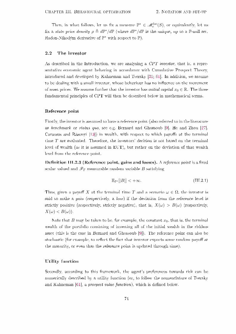
Chapter III. Behavioural optimisation 2. Notation and set-up
Then, in what follows, let us x a measure P∗ ∈ M loce (S), or equivalently, let us
x a state price density ρ , dP∗/dP (where dP∗/dP is the unique, up to a P-null set,Radon-Nikodým derivative of P∗ with respect to P).
2.2 The investor
As described in the Introduction, we are analysing a CPT investor, that is, a repre-
sentative economic agent behaving in accordance with Cumulative Prospect Theory,
introduced and developed by Kahneman and Tversky [31; 61]. In addition, we assume
to be dealing with a small investor, whose behaviour has no inuence on the movement
of asset prices. We assume further that the investor has initial capital x0 ∈ R. The threefundamental principles of CPT will then be described below in mathematical terms.
Reference point
Firstly, the investor is assumed to have a reference point (also referred to in the literature
as benchmark or status quo, see e.g. Bernard and Ghossoub [9], He and Zhou [27],
Carassus and Rásonyi [13]) in wealth, with respect to which payos at the terminal
time T are evaluated. Therefore, the investors' decision is not based on the terminal
level of wealth (as it is assumed in EUT), but rather on the deviation of that wealth
level from the reference point.
Denition III.2.3 (Reference point, gains and losses). A reference point is a xed
scalar-valued and FT -measurable random variable B satisfying
EP∗ [|B|] < +∞. (III.2.1)
Thus, given a payo X at the terminal time T and a scenario ω ∈ Ω, the investor is
said to make a gain (respectively, a loss) if the deviation from the reference level is
strictly positive (respectively, strictly negative), that is, X(ω) > B(ω) (respectively,
X(ω) < B(ω)).
Note that B may be taken to be, for example, the constant x0, that is, the terminal
wealth of the portfolio consisting of investing all of the initial wealth in the riskless
asset (this is the case in Bernard and Ghossoub [9]). The reference point can also be
stochastic (for example, to reect the fact that investor expects some random payo at
the maturity, or even that the reference point is updated through time).
Utility function
Secondly, according to this framework, the agent's preferences towards risk can be
numerically described by a utility function (or, to follow the nomenclature of Tversky
and Kahneman [61], a prospect value function), which is dened below.
74
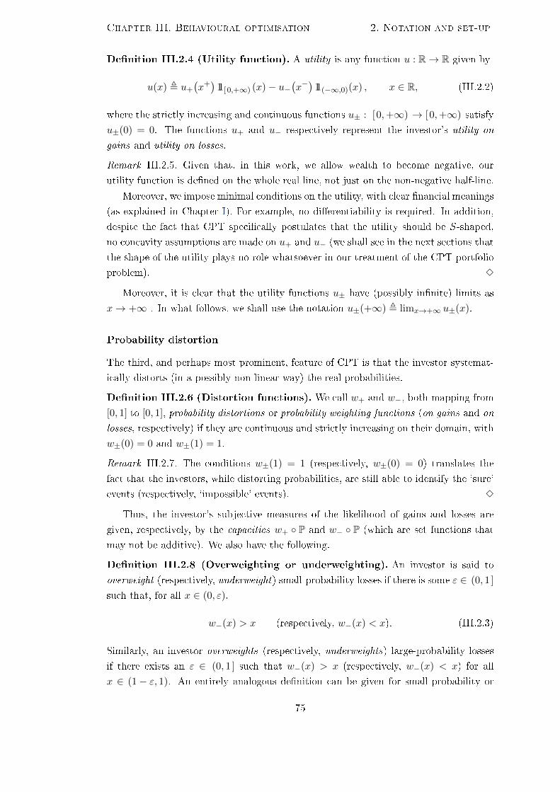
Chapter III. Behavioural optimisation 2. Notation and set-up
Denition III.2.4 (Utility function). A utility is any function u : R→ R given by
u(x) , u+
(x+)
11[ 0,+∞) (x)− u−(x−)
11(−∞,0)(x) , x ∈ R, (III.2.2)
where the strictly increasing and continuous functions u± : [0,+∞) → [0,+∞) satisfy
u±(0) = 0. The functions u+ and u− respectively represent the investor's utility on
gains and utility on losses.
Remark III.2.5. Given that, in this work, we allow wealth to become negative, our
utility function is dened on the whole real line, not just on the non-negative half-line.
Moreover, we impose minimal conditions on the utility, with clear nancial meanings
(as explained in Chapter I). For example, no dierentiability is required. In addition,
despite the fact that CPT specically postulates that the utility should be S -shaped,
no concavity assumptions are made on u+ and u− (we shall see in the next sections that
the shape of the utility plays no role whatsoever in our treatment of the CPT portfolio
problem). 3
Moreover, it is clear that the utility functions u± have (possibly innite) limits as
x→ +∞ . In what follows, we shall use the notation u±(+∞) , limx→+∞ u±(x).
Probability distortion
The third, and perhaps most prominent, feature of CPT is that the investor systemat-
ically distorts (in a possibly non-linear way) the real probabilities.
Denition III.2.6 (Distortion functions). We call w+ and w−, both mapping from
[0, 1] to [0, 1], probability distortions or probability weighting functions (on gains and on
losses, respectively) if they are continuous and strictly increasing on their domain, with
w±(0) = 0 and w±(1) = 1.
Remark III.2.7. The conditions w±(1) = 1 (respectively, w±(0) = 0) translates the
fact that the investors, while distorting probabilities, are still able to identify the `sure'
events (respectively, `impossible' events). 3
Thus, the investor's subjective measures of the likelihood of gains and losses are
given, respectively, by the capacities w+ P and w− P (which are set functions that
may not be additive). We also have the following.
Denition III.2.8 (Overweighting or underweighting). An investor is said to
overweight (respectively, underweight) small-probability losses if there is some ε ∈ (0, 1]
such that, for all x ∈ (0, ε),
w−(x) > x (respectively, w−(x) < x). (III.2.3)
Similarly, an investor overweights (respectively, underweights) large-probability losses
if there exists an ε ∈ (0, 1] such that w−(x) > x (respectively, w−(x) < x) for all
x ∈ (1− ε, 1). An entirely analogous denition can be given for small-probability or
75
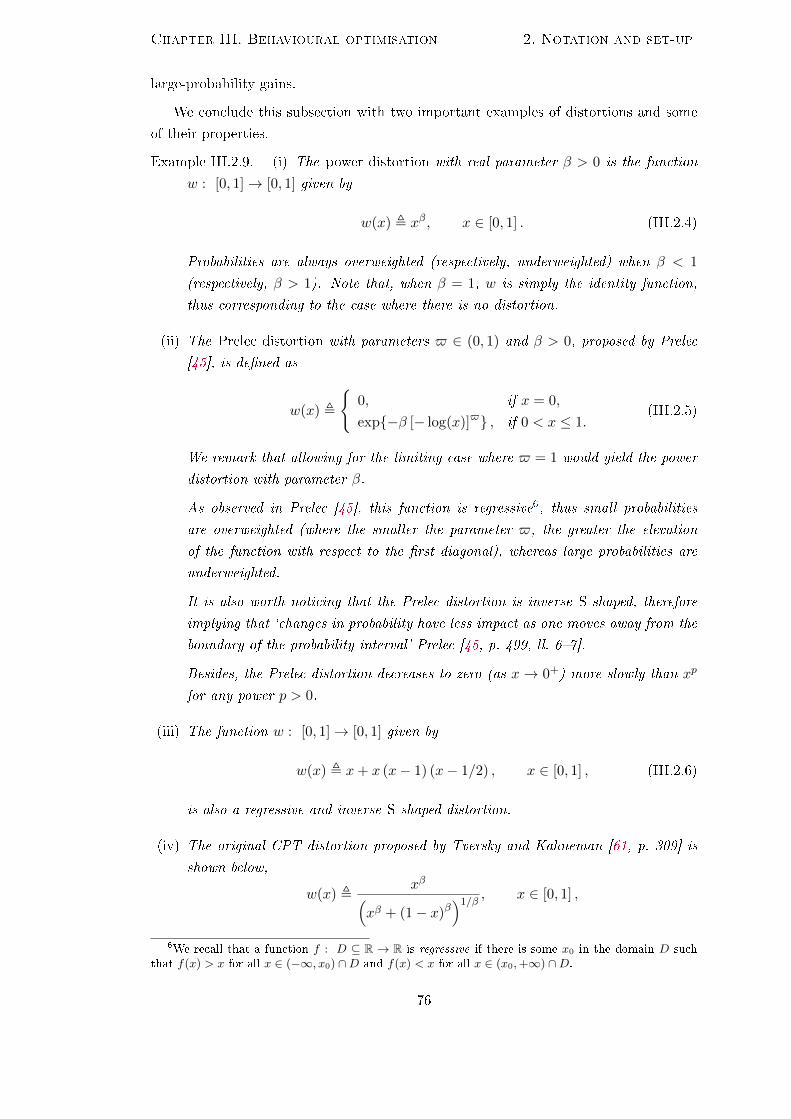
Chapter III. Behavioural optimisation 2. Notation and set-up
large-probability gains.
We conclude this subsection with two important examples of distortions and some
of their properties.
Example III.2.9. (i) The power distortion with real parameter β > 0 is the function
w : [0, 1]→ [0, 1] given by
w(x) , xβ, x ∈ [0, 1] . (III.2.4)
Probabilities are always overweighted (respectively, underweighted) when β < 1
(respectively, β > 1). Note that, when β = 1, w is simply the identity function,
thus corresponding to the case where there is no distortion.
(ii) The Prelec distortion with parameters $ ∈ (0, 1) and β > 0, proposed by Prelec
[45], is dened as
w(x) ,
0, if x = 0,
exp−β [− log(x)]$ , if 0 < x ≤ 1.(III.2.5)
We remark that allowing for the limiting case where $ = 1 would yield the power
distortion with parameter β.
As observed in Prelec [45], this function is regressive6, thus small probabilities
are overweighted (where the smaller the parameter $, the greater the elevation
of the function with respect to the rst diagonal), whereas large probabilities are
underweighted.
It is also worth noticing that the Prelec distortion is inverse S-shaped, therefore
implying that `changes in probability have less impact as one moves away from the
boundary of the probability interval' Prelec [45, p. 499, ll. 67].
Besides, the Prelec distortion decreases to zero (as x→ 0+) more slowly than xp
for any power p > 0.
(iii) The function w : [0, 1]→ [0, 1] given by
w(x) , x+ x (x− 1) (x− 1/2) , x ∈ [0, 1] , (III.2.6)
is also a regressive and inverse S-shaped distortion.
(iv) The original CPT distortion proposed by Tversky and Kahneman [61, p. 309] is
shown below,
w(x) ,xβ(
xβ + (1− x)β)1/β
, x ∈ [0, 1] ,
6We recall that a function f : D ⊆ R → R is regressive if there is some x0 in the domain D suchthat f(x) > x for all x ∈ (−∞, x0) ∩D and f(x) < x for all x ∈ (x0,+∞) ∩D.
76

Chapter III. Behavioural optimisation 2. Notation and set-up
where β ∈ (0, 1). Note that this function is inverse S-shaped. Additionally, it
follows from the trivial inequality (II.5.1) that w(x) ≤ xβ for every x ∈ [0, 1].
On the other hand, it is straightforward to check that w(x) ≥ 21−1/βxβ. The
mathematical treatment of this distortion can then turn out to be equivalent to (i)
above.
2.3 The optimal portfolio problem
In order to characterise how a CPT investor makes decisions in the face of uncertainty,
we must start with the following.
Denition III.2.10 (Prospect functional). Given any FT -measurable random vari-
able X : Ω→ R, let us denote by V±(X±) the Choquet integral of u±X± with respect
to the capacity w± P, that is,
V±(X±),∫ +∞
0w±(Pu±(X±)> y)
dy. (III.2.7)
Then, whenever V+(X+) < +∞ or V−(X−) < +∞, we dene the prospect functional
of X as follows,
V (X) , V+
(X+)− V−
(X−), (III.2.8)
possibly taking the values +∞ or −∞.
Remark III.2.11. (i) An important observation is that the presence of the probability
distortions w± leads to the appearance of the capacities w± P (not necessarily
additive), which in turn results in the involvement of the Choquet integrals V±(not necessarily linear).
(ii) Note that, as remarked in Remark C.5, in the case where there are no probability
distortions, that is, when w±(x) = x for Lebesgue-a.e. x ∈ [0, 1], we have that the
equalities
V±(X±)
= EP[u±(X±)]
hold for any random variable X. Therefore, the prospect functional V can be
regarded as a generalisation of the expected utility, and so our work covers the
classic EUT portfolio optimisation. 3
Now, we recall that, when evaluating a certain portfolio φ in the absence of con-
sumption, a CPT investor is not concerned about the terminal wealth ΠφT (as it was
assumed in EUT), but with the gain variable ΠφT − B (which can also take negative
values, thus representing a loss).
Next, in order to be able to study the optimisation problem, we must specify the
family of all suitable trading strategies, A (x0). Because the investor is assumed to have
an initial wealth of x0, we restrict ourselves to the set of trading strategies φ in Ψ for
which Πφ0 = x0. Another minimal assumption on the set of strategies is concerned with
77

Chapter III. Behavioural optimisation 2. Notation and set-up
the Choquet integrals V+
([ΠφT −B
]+)and V−
([ΠφT −B
]−). In order to ensure that
the prospect functional V given by (III.2.8) exists or is well-dened, we must require that
either one of the aforementioned integrals is nite. All the above can be summarised
below.
Denition III.2.12 (Feasible portfolios). A strategy φ ∈ Ψ is said to be allowable
or feasible for the behavioural portfolio problem (BPP) if it belongs to
A (x0) ,φ ∈ Ψ: Πφ
0 = x0 a.s. and V(
ΠφT −B
)is well-dened
. (III.2.9)
We call A (x0) the feasible set (or set of feasible portfolios).
Remark III.2.13. Whenever X is a claim admitting a replicating portfolio that belongs
to the set A (x0), by abuse of language we may write `X is in A (x0)' or `X is feasible
for (BPP)'. 3
Consequently, the nite-horizon portfolio choice problem for an investor with CPT
preferences consists of selecting the optimal trading strategies, from the set A (x0) of all
suitable portfolios (to be formally characterised later on), in terms of maximising the ex-
pected distorted payo functional V(
ΠφT −B
), which is written below in mathematical
terms.
Denition III.2.14 (Behavioural portfolio choice problem). The behavioural
portfolio problem with initial wealth x0 ∈ R on a nite horizon T ∈ (0,+∞) is written
as
supV(
ΠφT −B
): φ ∈ A (x0)
. (BPP)
Setting v∗(x0) , supV(
ΠφT −B
): φ ∈ A (x0)
, we say that φ
∗ ∈ A (x0) is an optimal
strategy if
v∗(x0) = V(
Πφ∗
T −B). (III.2.10)
Remark III.2.15. For a short discussion on the signicance of the existence of an optimal
strategy, once again see Remark II.2.21.
With regard to the conditions u±(0) = 0, these are imposed for convenience only
(cf. Remark II.4.2). 3
To conclude this subsection, we notice that, in general, when studying optimisation
problems such as (BPP) above, some issues may arise. In fact, rst of all, it may
happen that the supremum in (BPP) is innite, in which case maximisation does not
make sense. Intuitively speaking, it means that the investor can obtain an arbitrarily
high degree of satisfaction from the trading strategies that are available in the market.
For this reason, we introduce the following notion.
Denition III.2.16 (Well-posedness). A maximisation problem is termed well-posed
if its supremum is nite. Problems that are not well-posed are said to be ill-posed.
Secondly, even if the optimisation problem (BPP) is well-posed, it may still happen
78

Chapter III. Behavioural optimisation 2. Notation and set-up
that an optimal solution does not exist. Considering this, we state the following.
Denition III.2.17 (Attainability). A well-posed optimisation problem is said to be
attainable if it admits an optimal solution.
Addressing these issues will be the purpose of the subsequent sections.
2.4 Toy example: one-period binomial model (revisited)
In order to illustrate the importance of the changes introduced by CPT with respect to
EUT in the portfolio optimisation problem, let us return to the binomial market model
of Subsection II.2.4.
It is a well-known fact that this model is not only arbitrage-free, but also complete.
Moreover, the unique EMM is given by P∗(1) = (1− l) / (h− l) ∈ (0, 1).
Finally, assume that the investor has initial wealth x0 = 0 and reference point B = 0.
Since we allow wealth to become negative, it is then trivial that the set of admissible
portfolios coincides with that of self-nancing portfolios, which is in turn equal to
Φ(0) =(φ0, φ1
)∈ R2: φ0 = −φ1
.
We now study three interesting cases. In each gure, we shall plot the function to be
maximised as a function of φ1.
Case 1 Firstly, let us suppose that the investor has (negative) exponential utility with
parameter α = 1, that is,
u+(x) , 1− e−x and u−(x) , ex − 1,
for all x ∈ [0,+∞) . Also, let us take the market parameters h = 3/2, l = 1/2 and
p = 1/2, exactly as before. Given that the utility is globally concave, it is trivial that
the EUT portfolio choice problem is the following concave maximisation problem,
v∗(0) = sup
1
2
(1− e−φ1/2
)+
1
2
(1− eφ1/2
): φ1 ∈ R
,
with the unique solution φ∗
= (0, 0), as shown in Figure III.1a.
Let us now consider behavioural investors with the same exponential utility, and let
us assume that they distort the probabilities of gains and losses according to the power
functions below,
w+(x) , x1/4 and w−(x) , x1/2,
for all x ∈ [0, 1]. Then the investors would like to nd φ1 ∈ R maximising
V(φ1(S1
1 − 1))
=
(1/2)1/4(
1− eφ1/2)− (1/2)1/2
(e−φ
1/2 − 1), if φ1 < 0,
(1/2)1/4(
1− e−φ1/2)− (1/2)1/2
(eφ
1/2 − 1), if φ1 ≥ 0.
79
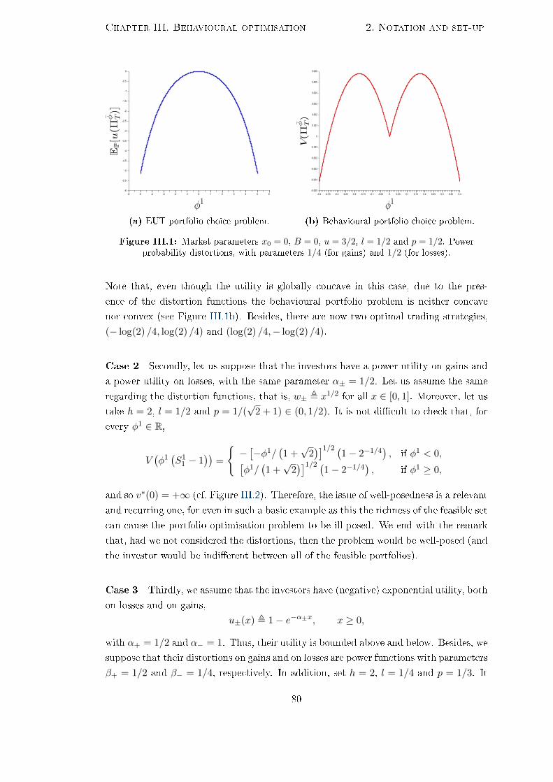
Chapter III. Behavioural optimisation 2. Notation and set-up
(a) EUT portfolio choice problem. (b) Behavioural portfolio choice problem.
Figure III.1: Market parameters x0 = 0, B = 0, u = 3/2, l = 1/2 and p = 1/2. Powerprobability distortions, with parameters 1/4 (for gains) and 1/2 (for losses).
Note that, even though the utility is globally concave in this case, due to the pres-
ence of the distortion functions the behavioural portfolio problem is neither concave
nor convex (see Figure III.1b). Besides, there are now two optimal trading strategies,
(− log(2) /4, log(2) /4) and (log(2) /4,− log(2) /4).
Case 2 Secondly, let us suppose that the investors have a power utility on gains and
a power utility on losses, with the same parameter α± = 1/2. Let us assume the same
regarding the distortion functions, that is, w± , x1/2 for all x ∈ [0, 1]. Moreover, let us
take h = 2, l = 1/2 and p = 1/(√
2 + 1) ∈ (0, 1/2). It is not dicult to check that, for
every φ1 ∈ R,
V(φ1(S1
1 − 1))
=
−[−φ1/
(1 +√
2)]1/2 (
1− 2−1/4), if φ1 < 0,[
φ1/(1 +√
2)]1/2 (
1− 2−1/4), if φ1 ≥ 0,
and so v∗(0) = +∞ (cf. Figure III.2). Therefore, the issue of well-posedness is a relevant
and recurring one, for even in such a basic example as this the richness of the feasible set
can cause the portfolio optimisation problem to be ill-posed. We end with the remark
that, had we not considered the distortions, then the problem would be well-posed (and
the investor would be indierent between all of the feasible portfolios).
Case 3 Thirdly, we assume that the investors have (negative) exponential utility, both
on losses and on gains,
u±(x) , 1− e−α±x, x ≥ 0,
with α+ = 1/2 and α− = 1. Thus, their utility is bounded above and below. Besides, we
suppose that their distortions on gains and on losses are power functions with parameters
β+ = 1/2 and β− = 1/4, respectively. In addition, set h = 2, l = 1/4 and p = 1/3. It
80

Chapter III. Behavioural optimisation 3. General results
Figure III.2: Ill-posed behavioural portfolio choice problem. Market parameters h = 2,l = 1/2 and p = 1/(
√2 + 1). Power distortions and power utilities, with parameter 1/2.
is straightforward to check that the investors aim to maximise
V(φ1(S1
1 − 1))
=
(2/3)1/2(
1− e3φ1/8)− (1/3)1/4
(1− eφ1
), if φ1 < 0,
(1/3)1/2(
1− e−φ1/2)− (2/3)1/4
(1− e−3φ1/4
), if φ1 ≥ 0,
over φ1 ∈ R. It is trivial that, in this case, v∗(0) = (2/3)1/2 − (1/3)1/4, so the problem
is well-posed, and yet no optimal portfolio exists (as can be intuited from Figure III.3).
Figure III.3: Non-attainable behavioural portfolio choice problem. Market parametersh = 2, l = 1/4 and p = 1/3. Power distortions and (negative) exponential utilities.
3 General results in continuous time
In this section, as well as in the remaining ones of this chapter, we shall assume that
trading occurs continuously in time, and thus T , [0, T ]. Furthermore, we assume that
81

Chapter III. Behavioural optimisation 3. General results
the process S is càdlàg, and that the ltration F = Ft: t ∈ [0, T ] satises the usual
conditions of saturatedness and right-continuity. Also, we recall that the alternative
characterisation (II.2.4) of the self-nancing condition in discrete time can be extended
to continuous-time markets as shown.
Denition III.3.1 (Self-nancing portfolio). A self-nancing portfolio is a d + 1-
dimensional, F-predictable stochastic process φ =φt =
(φ0t , φ>t
)>; t ∈ [0, T ]
, with
φt =(φ1t , . . . , φ
dt
)>, which is
(S0, S
)-integrable and whose associated wealth process
Πφ =
Πφt ; t ∈ [0, T ]
, given by Πφ
t ,∑d
i=0 φitSit , fullls the self-nancing condition
∀ t ∈ [0, T ] , Πφt = Πφ
0 +
∫ t
0φs dSs a.s.. (III.3.1)
The family of all self-nancing strategies is denoted by Φ.
Example III.3.2. We recover the trivial portfolio of (II.2.15), now in continuous time.
As before, ϕx0consists in investing all of the wealth on the riskless asset and none on
the risky assets, i.e.,
(ϕx0)0t , x0 and (ϕx0)it , 0,
for all t ∈ [0, T ] and i ∈ 1, . . . , d. Then its wealth process equals Πϕx0t = x0 for all
t ∈ [0, T ].
Next, it is a well-established fact in the literature that, without any further restric-
tions on the set of self-nancing portfolios, such arbitrage opportunities as doubling
schemes or suicide strategies (see, e.g., Harrison and Pliska [26]) can be found in the
market. There are several approaches to ruling out these pathologies, one of the most
frequent in the literature (and employed e.g. in Berkelaar et al. [8], Jin and Zhou [29],
and Carlier and Dana [15]) being that the (discounted) wealth process of any portfolio
should be bounded below by a constant (possibly depending on the portfolio). Although
this restriction, which reects the existence of a credit limit, is not an unrealistic one, it
looks rather unnatural when we take into account what was explained in Section III.1.
Therefore, in this work, we choose to adopt the following.
Denition III.3.3 (Admissible strategy). A self-nancing trading strategy is said
to be admissible if its (discounted) wealth process is a martingale under P∗ (and not
only a local martingale). We represent by Ψ the set of admissible strategies.
Remark III.3.4. The usual admissibility criterion has the advantage that it is invariant
with respect to the EMM, whereas ours depends on the P∗ we xed above. 3
Moreover, the following two assumptions will be in force throughout. The rst one
has to do with the reference point. As said before, B can be constant, deterministic
or stochastic, but its evolution must be known in some way, which mathematically
speaking means imposing the following.
Assumption III.3.5. The reference point B is hedgeable.
82

Chapter III. Behavioural optimisation 3. General results
Remark III.3.6. As noted in Jin and Zhou [29, Remark 2.1], given that B admits a
replicating portfolio φB ∈ Ψ by virtue of Assumption III.3.5, the optimal portfolio
problem can be reduced, for simplicity and without loss of generality, to one with
reference level equal to zero (and possibly dierent initial capital). Indeed, dening the
constant y0 , x0−EP∗ [B], it is trivial that a portfolio φ∗ ∈ A (x0) is optimal for (BPP)
with initial wealth x0 and reference point B if and only if φ∗ − φB ∈ A (y0) is optimal
for (BPP) with starting capital y0 and reference point equal to zero. Basically, as noted
also in Reichlin [52, Chapter II, Remark 2.5], the investor buys today the hedging
portfolio for B for the price EP∗ [B], and then attempts to allocate the remaining wealth
x0 − EP∗ [B] in an optimal way. 3
The second assumption is a kind of completeness hypothesis on the market, although
for a certain type of claims only.
Assumption III.3.7. All random variables in L1(Ω, σ(ρ) ,P∗) are hedgeable.
Remark III.3.8. It is worth noticing that Assumption III.3.7 is weaker (if only slightly)
than the usual notion of market completeness. Indeed, let us suppose that our market
model is complete, and consider an arbitrary claimX ∈ L1(Ω, σ(ρ) ,P∗). It is immediate
that P∗ is the only ELMM for S. Moreover, it is obvious that each
Xn , X 11|X|≤n + n 11X>n − n 11X<−n,
with n ∈ N, belongs to L∞(Ω,FT ,P) (recall that σ(ρ) ⊆ FT ), thus by completeness of
the market we have that, for some xn ∈ R and some admissible strategy φn,
Xn = xn +
∫ T
0φnt dSt a.s..
Now, setting x , EP∗ [X] (which is a real number, since EP∗ [|X|] < +∞ by hypothesis),
it is not dicult to check (using Lebesgue's Dominated Convergence Theorem) that the
sequence of stochastic integrals∫ T
0 φnt dSt; n ∈ Nconverges strongly (hence weakly)
in L1(Ω,FT ,P∗) to X−x. In addition, it can be shown that, for every xed n ∈ N, themartingale
∫ t0 φ
ns dSs; t ∈ [0, T ]
is uniformly integrable. Therefore, we may invoke
Corollary 2.5.2 in Yor [64] to deduce the existence of an admissible process φ such that
X − x =∫ T
0 φt dSt a.s., that is, X is hedgeable.
Hence, it is clear that our Assumption III.3.7 holds within a complete market frame-
work, but it can also be satised for incomplete nancial models, as shown by the
example provided in the upcoming Subsection III.3.4. 3
We shall also require that both ρ and 1/ρ should have moments of all strictly positive
orders, which will be needed frequently.
Assumption III.3.9. Both ρ and 1/ρ belong to W , where W is dened as in (II.4.5)
(i.e., it is the family of all real-valued and FT -measurable random variables Y satisfying
EP[|Y |p] < +∞ for all p > 0).
83
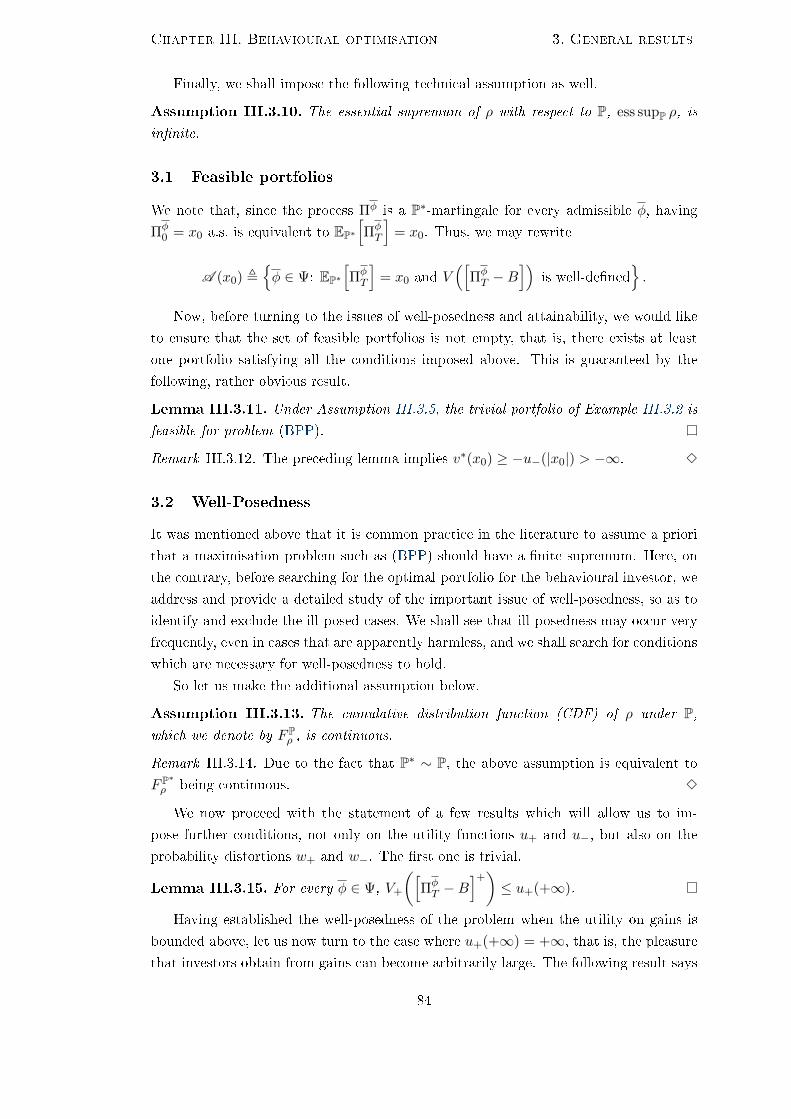
Chapter III. Behavioural optimisation 3. General results
Finally, we shall impose the following technical assumption as well.
Assumption III.3.10. The essential supremum of ρ with respect to P, ess supP ρ, is
innite.
3.1 Feasible portfolios
We note that, since the process Πφ is a P∗-martingale for every admissible φ, having
Πφ0 = x0 a.s. is equivalent to EP∗
[ΠφT
]= x0. Thus, we may rewrite
A (x0) ,φ ∈ Ψ: EP∗
[ΠφT
]= x0 and V
([ΠφT −B
])is well-dened
.
Now, before turning to the issues of well-posedness and attainability, we would like
to ensure that the set of feasible portfolios is not empty, that is, there exists at least
one portfolio satisfying all the conditions imposed above. This is guaranteed by the
following, rather obvious result.
Lemma III.3.11. Under Assumption III.3.5, the trivial portfolio of Example III.3.2 is
feasible for problem (BPP).
Remark III.3.12. The preceding lemma implies v∗(x0) ≥ −u−(|x0|) > −∞. 3
3.2 Well-Posedness
It was mentioned above that it is common practice in the literature to assume a priori
that a maximisation problem such as (BPP) should have a nite supremum. Here, on
the contrary, before searching for the optimal portfolio for the behavioural investor, we
address and provide a detailed study of the important issue of well-posedness, so as to
identify and exclude the ill-posed cases. We shall see that ill-posedness may occur very
frequently, even in cases that are apparently harmless, and we shall search for conditions
which are necessary for well-posedness to hold.
So let us make the additional assumption below.
Assumption III.3.13. The cumulative distribution function (CDF) of ρ under P,which we denote by F P
ρ , is continuous.
Remark III.3.14. Due to the fact that P∗ ∼ P, the above assumption is equivalent to
F P∗ρ being continuous. 3
We now proceed with the statement of a few results which will allow us to im-
pose further conditions, not only on the utility functions u+ and u−, but also on the
probability distortions w+ and w−. The rst one is trivial.
Lemma III.3.15. For every φ ∈ Ψ, V+
([ΠφT −B
]+)≤ u+(+∞).
Having established the well-posedness of the problem when the utility on gains is
bounded above, let us now turn to the case where u+(+∞) = +∞, that is, the pleasure
that investors obtain from gains can become arbitrarily large. The following result says
84
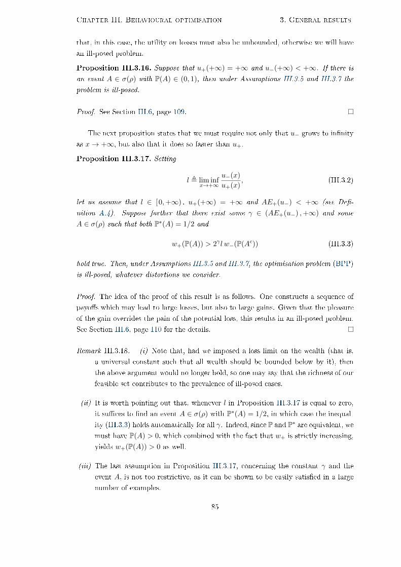
Chapter III. Behavioural optimisation 3. General results
that, in this case, the utility on losses must also be unbounded, otherwise we will have
an ill-posed problem.
Proposition III.3.16. Suppose that u+(+∞) = +∞ and u−(+∞) < +∞. If there is
an event A ∈ σ(ρ) with P(A) ∈ (0, 1), then under Assumptions III.3.5 and III.3.7 the
problem is ill-posed.
Proof. See Section III.6, page 109.
The next proposition states that we must require not only that u− grows to innity
as x→ +∞, but also that it does so faster than u+.
Proposition III.3.17. Setting
l , lim infx→+∞
u−(x)
u+(x), (III.3.2)
let us assume that l ∈ [0,+∞) , u+(+∞) = +∞ and AE+(u−) < +∞ (see De-
nition A.4). Suppose further that there exist some γ ∈ (AE+(u−) ,+∞) and some
A ∈ σ(ρ) such that both P∗(A) = 1/2 and
w+(P(A)) > 2γl w−(P(Ac)) (III.3.3)
hold true. Then, under Assumptions III.3.5 and III.3.7, the optimisation problem (BPP)
is ill-posed, whatever distortions we consider.
Proof. The idea of the proof of this result is as follows. One constructs a sequence of
payos which may lead to large losses, but also to large gains. Given that the pleasure
of the gain overrides the pain of the potential loss, this results in an ill-posed problem.
See Section III.6, page 110 for the details.
Remark III.3.18. (i) Note that, had we imposed a loss limit on the wealth (that is,
a universal constant such that all wealth should be bounded below by it), then
the above argument would no longer hold, so one may say that the richness of our
feasible set contributes to the prevalence of ill-posed cases.
(ii) It is worth pointing out that, whenever l in Proposition III.3.17 is equal to zero,
it suces to nd an event A ∈ σ(ρ) with P∗(A) = 1/2, in which case the inequal-
ity (III.3.3) holds automatically for all γ. Indeed, since P and P∗ are equivalent, wemust have P(A) > 0, which combined with the fact that w+ is strictly increasing,
yields w+(P(A)) > 0 as well.
(iii) The last assumption in Proposition III.3.17, concerning the constant γ and the
event A, is not too restrictive, as it can be shown to be easily satised in a large
number of examples.
85
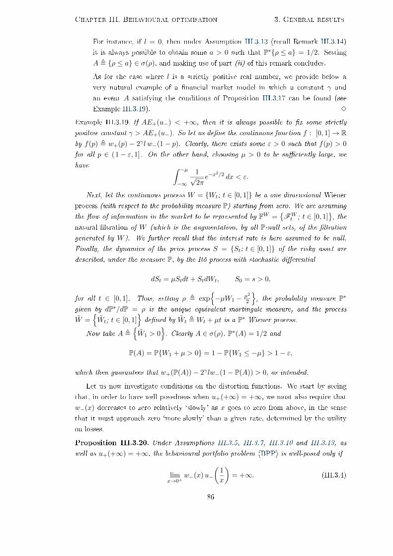
Chapter III. Behavioural optimisation 3. General results
For instance, if l = 0, then under Assumption III.3.13 (recall Remark III.3.14)
it is always possible to obtain some a > 0 such that P∗ρ ≤ a = 1/2. Setting
A , ρ ≤ a ∈ σ(ρ), and making use of part (ii) of this remark concludes.
As for the case where l is a strictly positive real number, we provide below a
very natural example of a nancial market model in which a constant γ and
an event A satisfying the conditions of Proposition III.3.17 can be found (see
Example III.3.19). 3
Example III.3.19. If AE+(u−) < +∞, then it is always possible to x some strictly
positive constant γ > AE+(u−). So let us dene the continuous function f : [0, 1]→ Rby f(p) , w+(p) − 2γl w−(1− p). Clearly, there exists some ε > 0 such that f(p) > 0
for all p ∈ (1− ε, 1] . On the other hand, choosing µ > 0 to be suciently large, we
have ∫ −µ−∞
1√2πe−x
2/2 dx < ε.
Next, let the continuous process W = Wt; t ∈ [0, 1] be a one-dimensional Wiener
process (with respect to the probability measure P) starting from zero. We are assuming
the ow of information in the market to be represented by FW =FWt ; t ∈ [0, 1]
, the
natural ltration of W (which is the augmentation, by all P-null sets, of the ltration
generated by W ). We further recall that the interest rate is here assumed to be null.
Finally, the dynamics of the price process S = St; t ∈ [0, 1] of the risky asset are
described, under the measure P, by the Itô process with stochastic dierential
dSt = µStdt+ StdWt, S0 = s > 0,
for all t ∈ [0, 1]. Thus, setting ρ , exp−µW1 − µ2
2
, the probability measure P∗
given by dP∗/dP = ρ is the unique equivalent martingale measure, and the process
W =Wt; t ∈ [0, 1]
dened by Wt ,Wt + µt is a P∗ Wiener process.
Now take A ,W1 > 0
. Clearly A ∈ σ(ρ), P∗(A) = 1/2 and
P(A) = PW1 + µ > 0 = 1− PW1 ≤ −µ > 1− ε,
which then guarantees that w+(P(A))− 2γlw−(1− P(A)) > 0, as intended.
Let us now investigate conditions on the distortion functions. We start by seeing
that, in order to have well-posedness when u+(+∞) = +∞, we must also require that
w−(x) decreases to zero relatively `slowly' as x goes to zero from above, in the sense
that it must approach zero `more slowly' than a given rate, determined by the utility
on losses.
Proposition III.3.20. Under Assumptions III.3.5, III.3.7, III.3.10 and III.3.13, as
well as u+(+∞) = +∞, the behavioural portfolio problem (BPP) is well-posed only if
limx→0+
w−(x)u−
(1
x
)= +∞. (III.3.4)
86
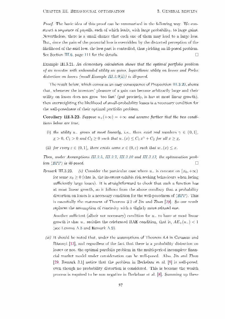
Chapter III. Behavioural optimisation 3. General results
Proof. The basic idea of this proof can be summarised in the following way. We con-
struct a sequence of payos, each of which leads, with large probability, to large gains.
Nevertheless, there is a small chance that each one of them may lead to a large loss.
But, since the pain of the potential loss is overridden by the distorted perception of the
likelihood of the said loss, the loss part is controlled, thus yielding an ill-posed problem.
See Section III.6, page 111 for the details.
Example III.3.21. An elementary calculation shows that the optimal portfolio problem
of an investor with unbounded utility on gains, logarithmic utility on losses and Prelec
distortion on losses (recall Example III.2.9(ii)) is ill-posed.
The result below, which comes as an easy consequence of Proposition III.3.20, shows
that, whenever the investors' pleasure of a gain can become arbitrarily large and their
utility on losses does not grow `too fast' (put precisely, it has at most linear growth),
then overweighting the likelihood of small-probability losses is a necessary condition for
the well-posedness of their optimal portfolio problem.
Corollary III.3.22. Suppose u+(+∞) = +∞ and assume further that the two condi-
tions below are true,
(i) the utility u− grows at most linearly, i.e., there exist real numbers γ ∈ (0, 1] ,
x > 0, C1 > 0 and C2 ≥ 0 such that u−(x) ≤ C1 xγ + C2 for all x ≥ x,
(ii) for every ε ∈ (0, 1], there exists some x ∈ (0, ε) such that w−(x) ≤ x.
Then, under Assumptions III.3.5, III.3.7, III.3.10 and III.3.13, the optimisation prob-
lem (BPP) is ill-posed.
Remark III.3.23. (i) Consider the particular case where u− is concave on [x0,+∞)
for some x0 ≥ 0 (that is, the investors exhibit risk seeking behaviours when facing
suciently large losses). It is straightforward to check that such a function has
at most linear growth, so it follows from the above corollary that a probability
distortion on losses is a necessary condition for the well-posedness of (BPP). This
is essentially the statement of Theorem 3.2 of Jin and Zhou [29]. So our result
replaces the assumption of concavity with a slightly more relaxed one.
Another sucient (albeit not necessary) condition for u− to have at most linear
growth is that u− satises the celebrated RAE condition, that is, AE+(u−) < 1
(see Lemma A.8 and Remark A.9).
(ii) It should be noted that, under the assumptions of Theorem 4.4 in Carassus and
Rásonyi [13], and regardless of the fact that there is a probability distortion on
losses or not, the optimal portfolio problem in the multi-period incomplete nan-
cial market model under consideration can be well-posed. Also, Jin and Zhou
[29, Remark 3.1] notice that the problem in Berkelaar et al. [8] is well-posed,
even though no probability distortion is considered. This is because the wealth
process is required to be non-negative in Berkelaar et al. [8]. Summing up these
87
Chapter III. Behavioural optimisation 3. General results
arguments, we are led to believe that ill-posedness in our continuous-time model
is likely to be due precisely to the richness of attainable payos (Carassus and
Rásonyi [13, Remark 4.10]), as well as to the absence of any constraints on the
wealth process. 3
With respect for the next result, it states in particular that, when the distortion on
gains w+ is going to zero (as x → 0+) `more slowly' than [u+(1/x)]−1, again we have
ill-posedness.
Proposition III.3.24. Under Assumptions III.3.5, III.3.7 and III.3.13, if
lim supx→0+
w+(x)u+
(1
x
)= +∞, (III.3.5)
then the problem is ill-posed.
Proof. The idea behind this proof involves constructing a sequence of payos which may
lead to small-probability large gains and whose large-probability losses are bounded
below by a universal constant. Therefore, the pain of losses is controlled, whereas the
pleasure of the potential gains can grow arbitrarily large (because the distortion on
gains cannot outbalance it). See Section III.6, page 111 for the details.
Remark III.3.25. (i) It is obvious that we have lim supx→0+ w+(x)u+(1/x) > 0 only
if u+(+∞) = +∞.
(ii) The nal observation in the proof of this result shows that it would still be valid
even if we imposed the constraint that the wealth should never fall below a certain
wealth oor. 3
Example III.3.26. An easy calculation shows that, when the investors have a power utility
and a Prelec distortion on gains, their optimal portfolio problem is ill-posed.
An immediate consequence of the preceding result is the following, which says that,
if the utility on gains grows `quickly' (namely, faster than linearly), then underweighting
the likelihood of small-probability gains is necessary for well-posedness.
Corollary III.3.27. Let us assume the following,
(i) there exist real numbers γ > 1, x > 0, C1 > 0 and C2 ≥ 0 such that the inequality
u+(x) ≥ C1 xγ + C2 is veried for all x ≥ x,
(ii) for every ε ∈ (0, 1], there exists some x ∈ (0, ε) such that w+(x) ≥ x.
Then, under Assumptions III.3.5, III.3.7 and III.3.13, the optimisation problem (BPP)
is ill-posed.
Remark III.3.28. We note that this corollary complements Theorem 3.2 of Jin and Zhou
[29] (and our Corollary III.3.22), but for the distortion on gains and when the utility
on gains has super-linear growth. 3
88

Chapter III. Behavioural optimisation 3. General results
The main necessary conditions for well-posedness obtained so far can be briey
compiled as follows.
Theorem III.3.29 (Necessary conditions, unbounded utility on gains). Suppose
u+(+∞) = +∞ and AE+(u−) < +∞. Then, under Assumptions III.3.5, III.3.7,
III.3.10 and III.3.13, the problem is well-posed only if the following three conditions are
simultaneously satised,
lim infx→+∞
u−(x)
u+(x)> 0, (III.3.6)
lim supx→0+
w+(x)u+
(1
x
)< +∞, (III.3.7)
limx→0+
w−(x)u−
(1
x
)= +∞. (III.3.8)
Remark III.3.30. (i) Note that our conditions (III.3.6) to (III.3.8) are completely in-
dependent of the shapes of the functions. In particular, no concavity assumptions
are needed, since what is really relevant for this discussion is the behaviour of
the utilities as x→ +∞, and that of the distortions for unlikely events (i.e., in a
right-neighbourhood of zero). In addition, we observe that none of the conditions
involve any market parameter, thus they are related (implicitly) to the market
model under consideration only through the set of allowable strategies.
(ii) Furthermore, not only are these conditions very easy to be checked, but they also
admit intuitive and nancial interpretations.
As a matter of fact, the rst condition means that the prospect value function is
steeper in the negative domain than in the positive one, or economically speak-
ing, that large losses are experienced more acutely than gains of the same order
of greatness, indicating loss aversion. When the limit in (III.3.6) exists, it cor-
responds to the LLAD measure introduced in He and Zhou [27]. We point out,
however, that unlike in the one-period model considered by He and Zhou [27, The-
orem 1], in our continuous-time market the condition limx→+∞ u−(x) /u+(x) =
+∞ alone is insucient to ensure well-posedness.
With regard to conditions (III.3.7) and (III.3.8), they reect the fact that the
investor's risk preferences and perceptions of reality, both on losses and on gains,
have to be well-adjusted or well-calibrated, in the sense that, for instance, the
distortion on losses cannot override the pain of a loss, nor can the distortion on
gains be overwhelmed by the pleasure of a gain.
(iii) Lastly, a careful inspection of the proofs reveals that, if either one of the con-
ditions (III.3.6) to (III.3.8) is not satised, then the maximisation problem is
ill-posed even if our set of feasible strategies is restricted to the ones which are
tame. 3
89
Chapter III. Behavioural optimisation 3. General results
3.3 Attainability
Let us now assume that the optimisation problem (BPP) is well-posed. As pointed out
in Section III.2, it may still happen nonetheless that the problem is not attainable. Our
aim is therefore to investigate the existence of an optimal trading strategy.
As before, Assumption III.3.5 will be in force. In addition, we introduce the following
concept.
Denition III.3.31 (Maximising sequence). We say that a sequence of feasible
portfoliosφn; n ∈ N
⊆ A (x0) is a maximising sequence for (BPP) if
v∗(x0) = limn→+∞
V(
ΠφnT −B
). (III.3.9)
Remark III.3.32. Obviously, by the denition of supremum, one can always nd at
least one such sequence. We note as well that the assumption of well-posedness and
Remark III.3.12 imply that v∗(x0) is a real number. Given that any real sequence
converging to a nite limit is bounded, in particular we get infn∈N V(
ΠφnT −B
)> −∞
for every maximising sequenceφn; n ∈ N
. 3
Henceforth, we shall impose the following important technical assumptions.
Assumption III.3.33. For every maximising sequenceφn; n ∈ N
,
supn∈N
V+
([ΠφnT
]+)< +∞. (III.3.10)
Assumption III.3.34. For every maximising sequenceφn; n ∈ N
, there exists an
integrable function g : [0,+∞) → [0,+∞) such that the inequality
w+
(Pu+
([ΠφnT
]+)> y
)≤ g(y) (III.3.11)
holds true for a.e. y ≥ 0.
Remark III.3.35. (i) Under Assumption III.3.5 and the assumption of well-posedness,
it is clear by the sub-additivity of the supremum that (III.3.10) implies
supn∈N
V−
([ΠφnT
]−)≤ sup
n∈NV+
([ΠφnT
]+)− infn∈N
V(
ΠφnT
)< +∞ (III.3.12)
(recall Remark III.3.32). Conversely, if (III.3.12) is true, then under the same
assumptions, supn∈N V+
([ΠφnT
]+)≤ supn∈N V
(ΠφnT
)+ supn∈N V−
([ΠφnT
]−)<
+∞. Hence, (III.3.10) and (III.3.12) are equivalent.
(ii) It is clear that Assumption III.3.34 will allow us to use, later on, the reverse Fatou
lemma. 3
So we are nally in the position to state the main result of this subsection, which
under certain conditions and whenever (BPP) is well-posed, establishes the existence of
90
Chapter III. Behavioural optimisation 3. General results
an optimal investment strategy.
Theorem III.3.36. Suppose that (BPP) is well-posed, and that Assumptions III.3.5,
III.3.7, III.3.9, III.3.13, III.3.33 and III.3.34 are in force. If for every maximising
sequenceφn; n ∈ N
there exists some constant η > 1 such that
supn∈N
EP
[([ΠφnT
]−)η]< +∞, (III.3.13)
then the problem (BPP) is attainable.
Proof. The intuition behind the proof can be summarised as follows. Firstly, we use
a compactness property (more specically, the tightness of the family of laws of the
terminal wealths of a maximising sequence of portfolios) to extract a limit distribution.
A natural candidate for an optimal portfolio is then one whose terminal wealth has the
said distribution. See Section III.6, page 112 for the details.
Remark III.3.37. Note that combining (III.3.13) with de la Vallée-Poussin's lemma
yields in particular that the sequence of losses of a maximising sequence is uniformly
integrable with respect to P. If, in addition, Assumption III.3.9 also holds, then this is
true under P∗ as well. 3
3.4 Examples
In this subsection we present two examples of important non-trivial market models to
which our results can be applied, for they verify the assumptions imposed above.
Multi-dimensional diusion model
Let k ∈ N, and let the continuous process W =Wt =
(W 1t , . . . ,W
kt
)>; t ∈ [0, T ]
,
taking values in Rk, be a k-dimensional Wiener process (with respect to P), which is
initialised at zero a.s.. As in Example III.3.19, we are considering the natural ltration
FW =FWt ; t ∈ [0, T ]
. We further recall that the interest rate is here assumed to be
null.
In this particular example, the price process of the i-th stock Si =Sit ; t ∈ [0, T ]
follows the stochastic dierential equation (SDE)
dSit = µitSitdt+
k∑j=1
σijt SitdW
jt , Si0 = si > 0, (III.3.14)
for any i ∈ 1, . . . , d. Here we assume that the coecients µi =µit; t ∈ [0, T ]
and
σi =σit =
(σi1t , . . . , σ
idt
)>; t ∈ [0, T ]
, respectively the appreciation rate process and
the Rd-valued volatility process of the i-th risky asset, are FW -adapted and satisfy∫ T0
∣∣µit∣∣ dt+ ∫ T0 ∑kj=1
∣∣∣σijt ∣∣∣2 dt < +∞ a.s., thus ensuring the existence and uniqueness of
strong solutions to the SDE (III.3.14). Finally, writing σt to denote the d× k volatility
91

Chapter III. Behavioural optimisation 3. General results
matrix with entries σijt , we assume that, for Lebesgue a.e. t ∈ [0, T ], σtσ>t is non-singular
a.s..
We study two cases separately.
Complete Market Let us suppose that there are as many risky assets as sources of
randomness, that is, k = d. Then it is trivial that there exists a uniquely determined d-
dimensional progressively measurable process θ =θt =
(θ1t , . . . , θ
dt
)>; t ∈ [0, T ]
such
that, for a.e. t ∈ [0, T ],
−µit =d∑j=1
σijt θjt a.s.
holds simultaneously for all i ∈ 1, . . . , d. In addition, let us further assume that the
condition 0 <∫ T
0
∑di=1
∣∣θit∣∣2 dt < +∞ is satised a.s. and that the strictly positive local
martingale ρt; t ∈ [0, T ] given by
ρt = exp
d∑i=1
∫ t
0θisdW
is −
1
2
∫ t
0
d∑i=1
∣∣θis∣∣2 ds
a.s.
is indeed a martingale under P. Hence, by the Cameron-Martin-Girsanov theorem and
its converse, it is well-known that the probability measure P∗, with Radon-Nikodým
derivative dP∗/dP = ρT a.s., is the unique ELMM for S, and the process dened by
W it = W i
t −∫ t
0 θis ds, for all t ∈ [0, T ] and i ∈ 1, . . . , d, is also a d-dimensional
Wiener process, but on the complete ltered probability space(Ω,FW
T ,FW ,P∗). Such
a nancial market is arbitrage-free and complete, hence any integrable contingent claim
is hedgeable (so Assumptions III.3.5 and III.3.7 are trivially true). Therefore, provided
that Assumptions III.3.9 and III.3.13 are satised, our Theorem III.3.36 applies. That
is, for example, the case when the market price of risk process θ is deterministic (in
which case it is straightforward to check that ρT is log-normally distributed both under
P and under P∗). The reader is also referred to Nualart [42, Chapter 2] for conditions
ensuring the existence of a continuous law for ρ.
Incomplete Market Assume now that 1 ≤ d < k, so there exist more sources of risk
than traded stocks. Moreover, in what follows, we shall consider only the case where all
coecients µi =µi(t) ; t ∈ [0, T ]
and σi =
σi(t) =
(σi1(t) , . . . , σid(t)
)>; t ∈ [0, T ]
are, as made explicit by the notation, deterministic Borelian functions of t. It is then
clear that a martingale measure for the d-dimensional process S is not unique. Indeed,
the system of linear equations
−µi(t) =
k∑j=1
σij(t) θj(t) , i ∈ 1, . . . , d , Lebesgue a.e. t ∈ [0, T ] , (III.3.15)
has innitely many solutions, and any Rk-valued process θ = θ(t) ; t ∈ [0, T ] satisfy-ing (III.3.15) denes a martingale measure P∗θ for S, under suitable conditions. There-
92

Chapter III. Behavioural optimisation 3. General results
fore, albeit admitting no arbitrage opportunities, the market is incomplete. Nonethe-
less, it is possible to construct a standard k-dimensional Brownian motion (with re-
spect to the probability measure P) starting at zero a.s., which we denote by W =Wt =
(W 1t , . . . , W
kt
)>; t ∈ [0, T ]
, whose natural ltration coincides with that of W
and such that the price process Si follows (under P) the dynamics
dSit = µi(t)Sitdt+
d∑j=1
σij(t)SitdWjt ,
for all i ∈ 1, . . . , d, where σ(t) =[σij(t)
]i,j∈1,...,d is a deterministic and invert-
ible square matrix of order d, for Lebesgue a.e. t ∈ [0, T ], with entries satisfying∫ T0
∑di,j=1
∣∣σij(t)∣∣2 dt < +∞. As a consequence, there exists a (unique) determinis-
tic process θ =θ(t) =
(θ1(t) , . . . , θd(t)
)>; t ∈ [0, T ]
, taking values in Rd, that solves
−µi(t) =∑d
j=1 σij(t) θj(t), for all i ∈ 1, . . . , d and for Lebesgue a.e. t ∈ [0, T ]. If
we impose the additional condition 0 <∫ T
0
∑di=1
∣∣θi(t)∣∣2 dt < +∞, then as above the
probability measure P∗ given by
dP∗
dP= exp
d∑i=1
∫ T
0θi(s) dW i
s −1
2
∫ T
0
d∑i=1
∣∣θi(s)∣∣2 ds a.s.,
is an ELMM for S, and the process W =
Wt =
(W 1t , . . . , W
kt
)>; t ∈ [0, T ]
, with
W it = W i
t −∫ t
0 θi(t) ds if i ∈ 1, . . . , d and W i
t = W it if i ∈ d+ 1, . . . , k, is a k-
dimensional Brownian motion on the probability space(Ω,FW
T ,P∗). Moreover, it is
clear that FW and the natural ltration of W agree, and that the Radon-Nikodým
derivative dP∗/dP is log-normally distributed (under the measures P and P∗), so again
Assumptions III.3.9, III.3.10 and III.3.13 are veried. Finally, let G = Gt; t ∈ [0, T ] be
the natural ltration of the Rd-valued Brownian motion
(W 1t , . . . , W
dt
)>; t ∈ [0, T ]
,
which is a sub-ltration of FW . It is obvious that dP∗/dP is measurable with respect to
GT , and that any GT -measurable and P∗-integrable random variable is hedgeable, hence
Assumption III.3.7 is valid (and weaker, if only slightly, than the standard notion of
market completeness).
A three-asset jump-diusion model with constant coecients
It is possible to construct examples of models with jumps to which Theorem III.3.36
applies, a very simple one being presented below.
Let us assume that the market contains a riskless asset with null interest rate, and
two risky assets whose price processes have dynamics given by
dS1t = S1
t−(σ1 dW
1t + ν dMt
), S1
0 = s1 > 0,
dS2t = S2
t−(µdt+ σ2 dW
2t
), S2
0 = s2 > 0,
93
Chapter III. Behavioural optimisation 4. Bounded utility
whereW 1,W 2 are two independent Wiener processes,M is the compensated martingale
associated with a Poisson process N with constant intensity λ (i.e., Mt , Nt − λ t,
t ∈ [0, T ]) which is independent of both W 1 and W 2, and where the coecients satisfy
µ 6= 0, σ1, σ2 > 0, and ν > −1 (note that this ensures that the price process S1 remains
strictly positive, since its jumps occur when N jumps and S1t = S1
t− (1 + ν∆Nt)).
Note that we are considering the ltration F to be the natural ltration of the triple(W 1,W 2,M
). We observe further that S1 is already a martingale with respect to the
historical probability measure.
It also is trivial to see that there exist innitely many ELMM for(S1, S2
), and thus
the market is not complete. Nevertheless, if we x the ELMM P∗ with Radon-Nikodým
density given bydP∗
dP= exp
− µ
σ2W 2T −
µ2
2σ22
T
a.s.,
it is obvious that all of the Assumptions III.3.7, III.3.9, III.3.10 and III.3.13 are ful-
lled. We do not enter into more details here as the examples we can construct in the
discontinuous case look rather articial.
4 Bounded utility on gains
The results presented in this section will appear in Rásonyi and Rodrigues [48].
As it is widely stated in the literature, the paper by Menger [37] (whose English
translation can be found in [38]) appears to have been the rst to assert the necessity
of a boundedness assumption on the utility function in order to avoid a St. Petersburg-
type paradox. Even though this has lead to a considerable amount of debate, several
authors have since advocated and made further arguments for considering bounded
utilities (see e.g. Arrow [4, 5, 6], Markowitz [36], and Savage [57], to cite only a few).
The existence in the real world of utilities which are unbounded above is peremptorily
dismissed as `absurd' by Muraviev and Rogers [41, footnote 3, p. 272], who provide a
strong argument against unbounded utilities (which they attribute to Kenneth Arrow).
In the light of the above, we shall make the following.
Assumption III.4.1 (Bounded utility on gains). The utility on gains is bounded,
i.e., u+(+∞) < +∞.
Remark III.4.2. Some of the best-known and most commonly used utilities in the liter-
ature satisfy this assumption, see Example II.2.15(i), (ii) and (v). 3
As Remark III.4.6 below shows, we cannot impose that the utility should be bounded
below as well, because this would contradict the existence of an optimiser.
4.1 Feasible portfolios
If follows easily from Lemma III.3.15 that, when the investors' utility is bounded above,
the feasible set consists of all admissible portfolios starting from initial wealth x0.
94

Chapter III. Behavioural optimisation 4. Bounded utility
Proposition III.4.3. Under Assumption III.4.1, A (x0) =φ ∈ Ψ: EP∗
[ΠφT
]= x0
.
4.2 Well-posedness
Another immediate consequence of Lemma III.3.15, as observed in the previous section,
is that well-posedness is trivial in our current setting (the best that can happen to the
investor is always bounded above).
Proposition III.4.4. Under Assumption III.4.1, v∗(x0) < +∞.
4.3 Attainability
It may still be the case that an optimal solution does not exist, so we must now study
whether or not the nite supremum v∗(x0) is indeed a maximum. A rst and important
answer is given by the following result.
Theorem III.4.5 (Necessary condition I). Under Assumptions III.3.5, III.3.7,
III.3.10 and III.3.13 and Assumption III.4.1, there exists an optimal portfolio for prob-
lem (BPP) only if
lim infx→0+
w−(x)u−
(1
x
)> 0. (III.4.1)
Proof. See Section III.6, page 116.
Remark III.4.6. (i) This result can be seen as the analogue of Proposition III.3.20,
but for bounded u+ and on the issue of attainability. We notice once more that
the necessary condition (III.4.1), involving only the losses, depends neither on
the market parameters nor on the shapes of the functions. Moreover, besides
being easy to verify, it has an evident nancial interpretation (already given in
Remark III.3.30).
(ii) In particular, Theorem III.4.5 implies that, if we have u−(+∞) < +∞ as well,
then the optimisation problem is not attainable. Although many authors argue
in favour of such u− (see e.g. Muraviev and Rogers [41]), for the remainder of this
section we shall only consider the case where u− is not bounded above.
(iii) Considering the specic case where both u− and w− are power functions, respec-
tively with parameters α− > 0 and β− > 0, there is an optimal strategy only if
α− ≥ β−. Moreover, trivial modications in the proof of Theorem III.4.5 show
that, when α− = β− (and thus limx→0+ w−(x)u−(1/x) = 1), existence of an
optimal portfolio still does not hold.
(iv) Another interesting conclusion which can be drawn is that, under additional con-
ditions on the growth of u−, the investor must overweight the likelihood of small-
probability losses, otherwise there is no optimal portfolio (the hypothesis on u−and the proof being exactly the same as those of Corollary III.3.22, except that
95

Chapter III. Behavioural optimisation 4. Bounded utility
now linear growth of u− is not allowed). This complements Theorem 3.2 of Jin
and Zhou [29], but for a bounded u+ and on the issue of attainability. 3
Example III.4.7. An investor with a logarithmic utility and a Prelec distortion on losses
does not admit an optimal trading strategy (cf. Example III.3.21).
Motivated by Theorem III.4.5, we introduce the following concept.
Denition III.4.8 (Associated distortion). Given a real number δ > 0 and a con-
tinuous, strictly increasing function u : [0,+∞) → [0,+∞) with u(+∞) = +∞, let us
dene the function wδu : [0, 1]→ [0, 1] in the following way,
wδu(x) ,
0, if x = 0,
[u(1) /u(1/x)]δ , if x ∈ (0, 1] .(III.4.2)
We call wδu the distortion associated with u with parameter δ.
Remark III.4.9. It is a trivial exercise to check that, for every appropriate choice of
u and δ, the function wδu dened above is continuous and strictly increasing on [0, 1],
with wδu(0) = 0 and wδu(0) = 0, whence a valid probability distortion. We note further
that investors having distortion wδu overweight (respectively, underweight) small proba-
bilities if their utility function veries u(x) < u(1)x1/δ (respectively, u(x) > u(1)x1/δ)
for suciently large x. Similarly, they underweight (respectively, overweight) large
probabilities whenever u(x) < u(1)x1/δ (respectively, u(x) > u(1)x1/δ) for all x in a
right-neighbourhood of 1. 3
Example III.4.10. (i) If u is a power function with parameter α > 0, then its asso-
ciated distortion with parameter δ > 0 is also a power function (with exponent
αδ > 0).
(ii) Let u be the utility of Example II.2.15(vii) with parameters α > 0 and $ ∈ (0, 1).
Then, for every δ > 0, its associated distortion is the Prelec distortion with pa-
rameters αδ > 0 and $ ∈ (0, 1).
The following corollary to Theorem III.4.5 is now immediate and tells us that, in
the particular case where the distortion on losses is the distortion associated with u−for some parameter δ > 0, a necessary condition for attainability is that δ ≤ 1.
Corollary III.4.11 (Necessary condition II). Let u−(+∞) = +∞ and δ > 0.
Suppose that the investor's probability weighting on losses satises
w−(x) ≤ wδu−(x) , x ∈ [0, 1] . (III.4.3)
Under Assumptions III.3.5, III.3.7, III.3.10 and III.3.13 and Assumption III.4.1, the
optimal portfolio problem (BPP) is attainable only if δ ≤ 1.
Therefore, when the parameter δ is strictly greater than 1, by the preceding result
we know that the supremum in (BPP) is never attained. The same conclusion also holds
with δ = 1 for some fairly typical utility functions (see Remark III.4.6(iii) above).
96
Chapter III. Behavioural optimisation 4. Bounded utility
The remainder of this section will be devoted to arguing that the condition δ < 1
is not only `almost necessary', but also sucient to ensure that an optimal trading
strategy does in fact exist, under an additional hypothesis on u− below.
Assumption III.4.12. For every δ ∈ (0, 1), there is some ξ > 1 such that
limx→+∞
[u−(xξ)]δ
u−(x)= 0. (III.4.4)
As an almost reciprocal of Corollary III.4.11, we have the following.
Theorem III.4.13 (Sucient condition). Suppose u− and wδu− are respectively as
in the statement of Corollary III.4.11 and Denition III.4.8, and that
w−(x) ≥ wδu−(x) , for all x ∈ [0, 1]. (III.4.5)
Under Assumptions III.3.5, III.3.7, III.3.9 and III.3.13, as well as Assumptions III.4.1
and III.4.12, if δ ∈ (0, 1), then there exists an optimal strategy.
Proof. See Section III.6, page 116.
Hence, Corollary III.4.11 and Theorem III.4.13 show that [u−(1/x)]−1 can be re-
garded as the threshold for the distortion function as far as the existence of an optimal
portfolio is concerned. Below this, in the sense of δ < 1, attainability holds. Above
this, when δ > 1 (or, for some cases, also when δ = 1), it does not.
Finally, the aim of the last result of this section is to show that, however articial
Assumption III.4.12 may seem at rst glance, it is actually associated with the renowned
concept of asymptotic elasticity.
Lemma III.4.14. Suppose u−(+∞) = +∞, and let z− : [0,+∞) → [0,+∞) be the
transform of u− given by z−(x) , log(u−(ex)), for all x ≥ 0. If there exist γ > 0 and
x > 0 such that
z−(λx) ≤ λγz−(x) , for all λ ≥ 1 and x ≥ x, (III.4.6)
then Assumption III.4.12 is satised.
Proof. See Section III.6, page 116.
Remark III.4.15. When z− is continuously dierentiable on (x0,+∞), for some x0 ≥0, we know by Proposition A.10 that condition (III.4.6) is equivalent to AE+(z−) <
+∞. 3
We nish this section with an important example demonstrating that Assump-
tion III.4.12 is satised by a large class of functions, namely it is true for some of
the most frequently considered utilities in the literature.
97

Chapter III. Behavioural optimisation 5. Power functions
Example III.4.16. (i) Suppose u− is continuously dierentiable and AE+(u−) < +∞.
If, in addition, there exist constants C > 0, γ > 0 such that u−(x) ≥ C xγ holds
true for all x suciently large, then u− satises Assumption III.4.12. Indeed,
x (z−)′(x)
z−(x)≤ x (z−)′(x)
log(C) + γx=
(z−)′(x)
(log(C) /x) + γ
for every suciently large x, therefore AE+(z−) ≤ γ−1 lim supx→+∞ (z−)′(x).
But, as noted in Kramkov and Schachermayer [35, p. 946], it is trivial to check
that lim supx→+∞ (z−)′(x) = AE+(u−), which is nite by hypothesis, hence the
claimed result is given by Lemma III.4.14.
In particular, this implies that the power utility function with parameter α > 0
(not necessarily strictly less than one), having asymptotic elasticity equal to α,
veries Assumption III.4.12. Moreover, so do the utilities of items (vi) and (viii)
of Example II.2.15, which have asymptotic utility 1.
(ii) Let u1 be the utility of Example II.2.15(vii) with parameters α > 0 and $ ∈ (0, 1),
u2 the logarithmic utility, and u3 the log-log utility. Their transforms, z1, z2
and z3, respectively, equal z1(x) = αx$, z2(x) = log(log(1 + ex)), and z3(x) =
log(log(1 + log(1 + ex))), for all x ≥ 0. It can be checked that these functions are
strictly concave, hence AE+(zi) ≤ 1 for all i ∈ 1, 2, 3 (see, e.g., Kramkov and
Schachermayer [35, Lemma 6.1]).
(iii) Assume u−(+∞) = +∞, and also that (u−)′ exists and tends to 0 fast enough as
x→ +∞, or more precisely, (u−)′(x) ≤ C [x log(x)]−1 for some C > 0 and for x
large enough. Then Assumption III.4.12 is fullled. Indeed,
lim supx→+∞
x (z−)′(x)
z−(x)= lim sup
x→+∞
x ex (u−)′(ex)
u−(ex) log(u−(ex))≤ lim
x→+∞
C
u−(ex) log(u−(ex))= 0.
5 Power utilities and distortions
Most of the material in this section has been published in the paper [47].
It was briey mentioned in Section III.4 that the requirement that utilities must be
bounded has not been unanimously accepted in the literature. On the contrary, there
are divided opinions, giving origin to some productive and resolute discussions (see, for
example, the paper by Ryan [54] and the response of Arrow [6]). One of the recurrent
objections to the assumption of boundedness is that it excludes power and logarithmic
utilities, two of the most often used functions in economics. Thus, many papers have
been dedicated to supporting and trying to accommodate the use of unbounded utilities
(we refer to the works, e.g., of Fishburn [24], Samuelson [56] and Toulet [60]). Hence,
having dealt with bounded utilities on gains in the preceding section, we now turn to
investors whose utility function is unbounded above. We then know by Section III.3 that
they must also have a utility function which is unbounded below (otherwise the problem
98

Chapter III. Behavioural optimisation 5. Power functions
is automatically ill-posed, see Proposition III.3.16). Inspired by Carassus and Rásonyi
[13], we shall focus our study on power-like utilities (with strictly positive parameters,
to ensure that the functions are strictly increasing).
Assumption III.5.1 (Power-like utilities). The investor has a piecewise power-like
utility function, that is, there exist strictly positive real numbers α+, α−, κ+ and κ−
such that, for all x ∈ [0,+∞) ,
u+(x) ≤ κ+xα+ and u−(x) ≥ κ−xα− . (III.5.1)
Remark III.5.2. This choice is not as articial or arbitrary as it may seem. Firstly, the
power utility is one of the most applied in nance and economics. Secondly, if we assume
that the utility on gains is a power function, then we know by Proposition III.3.17 that
taking for the utility on losses a function which grows more slowly than any strictly
positive power (such as the logarithmic or the log-log utilities) would inevitably lead,
under additional assumptions, to an ill-posed problem. Conversely, if u− is a power
function, then taking for u+ a function which grows more quickly than any strictly
positive power would also yield an ill-posed problem (again by Proposition III.3.17). 3
With regard to the distortions, and motivated by Denition III.4.8, we shall assume
that the investor's distortion on gains and distortion on losses behave like the distortions
associated with power functions. Recalling Example III.4.10(i), that means imposing
the following.
Assumption III.5.3 (Power-like distortions). The investor has power-like weight-
ing functions, i.e., there exist real numbers β+, β− > 0, k+ ≥ 1 and k− ∈ (0, 1] such
that,
w+(x) ≤ k+xβ+ and w−(x) ≥ k−xβ− . (III.5.2)
for all x ∈ [0, 1].
5.1 Well-posedness
Like in the preceding Section III.3, we are concerned with seeking conditions on the
parameters under which the portfolio problem is a well-posed one. In order to do so,
we shall make the additional assumption below.
Assumption III.5.4. The essential inmum of ρ with respect to P, ess infP ρ, is zero.
Then our rst result, which is a direct consequence of Theorem III.3.29 and of an
easy adaptation of its proof, essentially recovers Theorem 3.9 in Rásonyi and Rodrigues
[47], while also including the borderline cases α± = β±.
Theorem III.5.5 (Necessary conditions). Assume that both the utilities u+, u− and
the distortions w+, w− are power functions with strictly positive parameters α+, α−, β+
and β−, respectively. Suppose further that there exist a real number γ > α− and an
event A ∈ σ(ρ) verifying both P∗(A) = 1/2 and [P(A)]β+ > 2γ [1− P(A)]β−. Under As-
99

Chapter III. Behavioural optimisation 5. Power functions
sumptions III.3.5, III.3.7, III.3.10 and III.3.13 and Assumption III.5.4, the behavioural
portfolio problem (BPP) is well-posed only if
α+ < α− andα+
β+< 1 <
α−β−
. (III.5.3)
Proof. See Section III.6, page 117.
Remark III.5.6. (i) Again we stress that these conditions are extremely easy to verify
and are not associated with any of the market parameters.
(ii) The condition α+ < α− is also mentioned in Bernard and Ghossoub [9] and He and
Zhou [27] for one-period models, and in Carassus and Rásonyi [13] and Rásonyi
and Rodríguez-Villarreal [49] for multi-period markets. In particular, in He and
Zhou [27], the authors conclude that the restriction α+ < α− alone (without any
further conditions on the distortions) is enough to ensure well-posedness. This
statement is no longer true in our continuous-time market model.
(iii) The nancial meaning of the parameter restrictions given by (III.5.3) has already
been discussed in Remark III.3.30. Here we explore further some interesting spe-
cial cases.
Suppose that the investor is risk-seeking on losses (α− < 1). Thus, it follows from
loss aversion (the rst inequality in (III.5.3)) that investor must be risk-averse
when gaining (α+ < 1). Moreover, the investor needs to inate the probabilities
of losses occurring (β− < 1, cf. Corollary III.3.22). With respect to the distortion
on gains, we remark that all three cases β+ < 1 or β+ = 1 or β+ > 1 are possible
(so long as α+ < β+ holds).
On the other hand, it may happen that the investors exaggerate the likelihood of
gains (β+ < 1), in which case they must be risk-averse when gaining (α+ < 1).
Note, however, that we do not impose that the exponents must be strictly less
than one. In particular, we allow for the case where the investor is risk-neutral
or risk-seeking on gains (α+ ≥ 1), which in turn implies that the perceived prob-
abilities of gains must be no greater than the actual probabilities (β+ > 1, cf.
Corollary III.3.27). In addition, loss aversion gives that the investor cannot be
risk-seeking on losses (α− > 1).
Another possible case is that in which either there is no distortion on losses or the
investor underweights the probabilities of losses (β− ≥ 1). Then, the problem is
ill-posed unless the investor is risk-averse when losing (α− > 1).
In any case, the condition reecting loss aversion always introduces a kink in the
utility function at zero. What is more, the investor's utility must be steeper on
losses than on gains. 3
The rest of this subsection is devoted to the proof of the reciprocal of Theorem III.5.5,
and thus to showing that the inequalities in (III.5.3) above are sharp.
100
Chapter III. Behavioural optimisation 5. Power functions
Theorem III.5.7 (Sucient conditions). Under Assumption III.3.9 and Assump-
tions III.5.1 and III.5.3, if
α+ < α− andα+
β+< 1 <
α−β−
, (III.5.3)
then the behavioural portfolio problem (BPP) is well-posed.
Proof. See Section III.6, page 118.
Remark III.5.8. It is worth comparing Theorem III.5.7 to a result of Carassus and
Rásonyi [13]. In a discrete-time, multi-period market model, and adapting their notation
to ours, well-posedness is obtained in Carassus and Rásonyi [13, Theorem 4.4] whenever
α+
β+< α−, (III.5.4)
modulo some integrability conditions related to the price process. One can check, using
Proposition 7.1 of Rásonyi and Stettner [50], that the integrability conditions of Caras-
sus and Rásonyi [13] imply the existence of a risk-neutral measure P∗ ∼ P with dP∗/dPand dP/dP∗ in W , hence our Theorem III.5.7 ensures well-posedness also in the case
α+ < α− andα+
β+< 1 <
α−β−
. (III.5.3)
Note that (III.5.4) and (III.5.3) are incomparable conditions, as none of them implies the
other one. It is also worth emphasizing that the domains of optimization are dierent in
Carassus and Rásonyi [13] and in the present work. Hence, in the discrete-time multi-
period case, our Theorem III.5.7 complements, but does not subsume, the corresponding
results of Carassus and Rásonyi [13]. 3
5.2 Attainability
The last theorem of this section states that, if the parameters satisfy the inequalities in
(III.5.3), then under suitable assumptions not only is (BPP) well-posed, but also it is
attainable.
Theorem III.5.9. Suppose Assumptions III.3.5, III.3.7, III.3.9 and III.3.13 and As-
sumptions III.5.1 and III.5.3 are in force. If
α+ < α− andα+
β+< 1 <
α−β−
, (III.5.3)
then there is an optimal portfolio for (BPP).
Proof. See Section III.6, page 118.
Remark III.5.10. Our Theorems III.5.7 and III.5.9 apply, in particular, to the original
CPT distortion functions proposed by Tversky and Kahneman [61] with k+ = 1 and
k− = 21−1/β ∈ (0, 1] (recall Example III.2.9(iv)). 3
101
Chapter III. Behavioural optimisation 6. Proofs and auxiliary results
6 Proofs and auxiliary results
6.1 Auxiliary results
Unless otherwise stated, we stay in the setting of Section III.3.
Lemma III.6.1. Suppose Assumptions III.3.5, III.3.7, III.3.10 and III.3.13 hold true,
and set
l , lim infx→0+
w−(x)u−
(1
x
). (III.6.1)
If l < +∞, then v∗(x0) ≥ u+(+∞)− l.
Proof. Given that both w− and u− are non-negative functions, it is trivial that the
limit inferior in (III.6.1) must belong to [0,+∞]. Using the hypothesis that l < +∞,
it is possible to recursively construct a strictly decreasing sequence an; n ∈ N, whoseterms satisfy an ∈ (0, 1/n) and w−(an)u−(1/an) < l + 1/n for every n ∈ N. It is
also clear that this sequence must converge to zero as n goes to innity. Moreover, we
can use Assumption III.3.13 to nd, for every n ∈ N, some real number bn such that
Pρ ≤ bn = 1−an. We remark that, since ρ > 0 a.s., each bn must be strictly positive.
We further notice that strict monotonicity of an; n ∈ N implies that the sequence
bn; n ∈ N is strictly increasing. Lastly, we claim that limn→+∞ bn = +∞. Indeed,
denoting by b the supremum of bn; n ∈ N, the continuity from below of P yields
Pρ ≤ b ≥ P
(+∞⋃n=1
ρ ≤ bn
)= lim
n→+∞Pρ ≤ bn = 1− lim
n→+∞an = 1,
therefore we must have b = +∞ (otherwise b would be an essential upper bound for ρ,
thus contradicting Assumption III.3.10).
Now, for every n ∈ N, we dene the event An , ρ ≤ bn ∈ σ(ρ) (we remark that
P∗(An) ∈ (0, 1), because P and P∗ are equivalent measures), as well as the non-negative
and σ(ρ)-measurable random variable
Xn ,bn
2P∗(An)11An .
In addition, combining the continuity from below with the equivalence of P and P∗, itis straightforward to see that limn→+∞ P∗(An) = P∗
(⋃+∞n=1 ρ ≤ bn
)= 1, so
V+(Xn) = u+
(bn
2P∗(An)
)w+(P(An)) −−−−−→
n→+∞u+(+∞)w+(1) .
Next, let
Yn ,bn − 2x0
2P∗(Acn)11Acn ,
which is also σ(ρ)-measurable. Given that limn→+∞ bn = +∞ as seen above, there
exists an integer n0 such that bn > 2x0 for any n ≥ n0, thus Yn ≥ 0 for every n ≥ n0.
102
Chapter III. Behavioural optimisation 6. Proofs and auxiliary results
Furthermore, it follows from limn→+∞ (bn − 2x0) / (2bn) = 1/2 that there must be some
n1 ∈ N such that (bn − 2x0) / (2bn) < 1 for all n ≥ n1. Combining these facts with the
inequality P∗(Acn) = EP[ρ11Acn
]≥ bn P(Acn) and with the monotonicity of u− yields
V−(Yn) = u−
(bn − 2x0
2P∗(Acn)
)w−(P(Acn)) ≤ u−
(1
P(Acn)
)w−(P(Acn)) < l +
1
n
for every n ≥ max n0, n1.Hence, setting Zn , Xn−Yn, for n ∈ N, it is obvious that Zn is σ(ρ)-measurable, and
also that EP∗ [Zn] = x0 by construction. Besides, for every n ≥ n0, we have EP∗ [|Zn|] =
bn−x0 < +∞, therefore Zn is replicable from initial capital x0. Moreover, each Zn (for
n suciently large) is actually feasible for (BPP), because V−(Z−n ) = V−(Yn) < +∞(note that also V+(Z+
n ) = V+(Xn) < +∞). Finally, recalling that w+(1) = 1, we
obtain supn∈N V (Zn) ≥ lim infn→+∞ V (Zn) ≥ u+(+∞) − l, which implies the desired
inequality.
Lemma III.6.2. Under Assumption III.4.1, there exists an optimal portfolio for prob-
lem (BPP) only if v∗(x0) < u+(+∞).
Proof. Let us suppose that there exists a feasible portfolio φ∗ ∈ A (x0) such that
v∗(x0) = V (X∗), where X∗ , Πφ∗
T − B. Since u+ is assumed to be strictly increas-
ing, we have that ∅ = u+(X+∗ ) ≥ u+(+∞) =
⋂+∞n=1 u+(X+
∗ ) > u+(+∞)− 1/n.Thus, the continuity from above of the probability measure implies the existence of
some n0 ∈ N for which both Pu+(X+∗ ) > u+(+∞)− 1/n0 < 1 and u+(+∞)−1/n0 >
0 hold true.
As a consequence, 0 ≤ Pu+(X+∗ ) > y ≤ Pu+(X+
∗ ) > u+(+∞)− 1/n0 < 1 for
all y ∈[u+(+∞)− 1
n0, u+(+∞)
], whence
u+(+∞)− V (X∗) ≥ u+(+∞)− V+
(X+∗)
≥∫ u+(+∞)
u+(+∞)−1/n0
[1− w+
(Pu+
(X+∗)> y)]
dy > 0,
because w+ is assumed to be strictly increasing.
Lemma III.6.3. Let w be a distortion and u : [0,+∞) → [0,+∞) a utility such that
u(+∞) = +∞. Suppose f : [0,+∞) → [0,+∞) is a continuous and strictly increasing
function, satisfying both f(0) = 0 and f(+∞) = +∞. Then
w(Pf(X) > t) ≤ 1
u(f−1(t))
∫ +∞
0w(Pu(X) > y) dy (III.6.2)
for any t > 0 and for any random variable X ≥ 0.
Proof. Let t > 0 be arbitrary, but xed. Then, for any random variable X ≥ 0, we have
103

Chapter III. Behavioural optimisation 6. Proofs and auxiliary results
by the monotonicity of the integral, as well as that of u and f (and their inverses) that
∫ +∞
0w(Pu(X) > y) dy ≥
∫ u(f−1(t))
0w(Pf(X) > f
(u−1(y)
))dy
≥∫ u(f−1(t))
0w(Pf(X) > t) dy,
where the last inequality follows from the inclusion f(X) > t ⊆f(X) > f
(u−1(y)
)for all y ∈
[0, u(f−1(t)
)].
Corollary III.6.4. Suppose u is as in Lemma III.6.3, and let δ > 0 be arbitrary. Then
for every s > 0 we have
PXs > t ≤
u−1
u(1)
[u(t1/s)
V δu (X)
]1/δ−1
(III.6.3)
for all t > 0 and for all random variables X ≥ 0, where
V δu (X) ,
∫ +∞
0wδu(Pu(X) > y) dy (III.6.4)
and wδu is the associated distortion of Denition III.4.8.
Remark III.6.5. Note that, if X ≥ 0 and V δu (X) = 0, then X = 0 a.s. (see Proposi-
tion C.6(vi) and Remark C.7), and so (III.6.3) is trivially valid. 3
Lemma III.6.6. Let u be a utility function with u(+∞) = +∞. The following three
statements are equivalent,
(i) Assumption III.4.12 holds true for u,
(ii) for each δ ∈ (0, 1), there exist a real number ζ > 1 and a non-increasing function
G : (0,+∞)→ [1,+∞) such that, for every λ > 0,
u(xζ)≤ [λu(x)]1/δ , (III.6.5)
for all x ≥ G(λ),
(iii) for every δ ∈ (0, 1), there is ς > 1 for which limx→+∞ [z(x)− δ z(ςx)] = +∞,
where z is the transform of u dened in Lemma III.4.14.
Proof. We begin by showing (i)⇔(ii). To prove that (ii) implies (i), x δ ∈ (0, 1) and
let ε > 0 be arbitrary. Then, for all x ≥ G(ε/2) ≥ 1, we have[u(xζ)]δ
/u(x) ≤ ε/2,
and therefore limx→+∞[u(xζ)]δ
/u(x) = 0.
Now we prove the reverse implication. Again, let δ ∈ (0, 1) be xed, and consider an
arbitrary λ > 0. Since, by hypothesis, limx→+∞[u(xξ)]δ
/u(x) = 0, there exists some
L , L(λ) ≥ 1 such that u(xξ)< [λu(x)]1/δ for all x ≥ L. Next dene, for each λ > 0,
104

Chapter III. Behavioural optimisation 6. Proofs and auxiliary results
the non-empty set
Sλ ,L ≥ 1: u
(xξ)< [λu(x)]1/δ for all x ≥ L
,
which is bounded below by 1, so it admits an inmum. Then let G : (0,+∞) → R be
the function given by G(λ) , inf Sλ, for any λ > 0. Clearly, by construction, G ≥ 1.
Furthermore, it can be easily checked that, for every λ > 0 and for all x ≥ G(λ), the
inequality u(xξ)≤ [λu(x)]1/δ holds true. In fact, if x > G(λ), then by denition of
inmum, we can nd some M ∈ Sλ satisfying x > M , and thus u(xξ)< [λu(x)]1/δ.
So suppose, on the other hand, that x = G(λ). Again it follows from the denition of
inmum that there exists a sequence Mn; n ∈ N ⊆ Sλ such that limn∈NMn = x and
hence, by continuity, we obtain
u(xξ)
= limn→+∞
u(M ξn
)≤ lim
n→+∞[λu(Mn)]1/δ = [λu(x)]1/δ .
Finally, it remains to show that G is indeed a non-increasing function of λ. To see
this, let 0 < λ1 ≤ λ2. Then, for all x ≥ G(λ1) ≥ 1, we have u(xa) ≤ [λ1u(x)]1/δ ≤[λ2u(x)]1/δ, hence G(λ1) belongs to Sλ2 . Consequently, we must have, by the denition
of the inmum, that G(λ1) ≥ G(λ2).
We now prove (i)⇔ (iii). To show that (i) implies (iii), let us start by considering
an arbitrary M > 0. Then we can use the hypothesis to nd some x0 > 1 such that[u(eξx)]δ
/u(ex) < e−M holds true for all x ≥ x0, and applying logarithms to both sides
of the above inequality yields −M > δ z(ξx) − z(x). The reverse implication can also
be obtained in a straightforward and analogous manner.
Lemma III.6.7. Suppose u is a utility with u(+∞) = +∞ and satisfying Assump-
tion III.4.12. Let δ ∈ (0, 1), and let the non-increasing function G : (0,+∞)→ [1,+∞)
and the real number ζ > 1 be those given by Lemma III.6.6. Then, for every η ∈ (1, ζ),
there exist constants C > 0 and D > 0 such that, for all random variables X ≥ 0,
EP[Xη] ≤ C +
[G(D[V δu (X)
]−1)]η
u−1(D [V δ
u (X)]−1/δ
) , (III.6.6)
with V δu (X) given by (III.6.4).
Proof. Fix δ ∈ (0, 1) and η ∈ (1, ζ), and let X be any non-negative random variable.
If X = 0 a.s., then EP[Xη] = 0 and V δu (X) = 0 (by Proposition C.6(v)), hence the
inequality (III.6.6) is satised trivially for any C > 0 and D > 0. So suppose now
that PX > 0 > 0, which implies V δu (X) > 0 (by Proposition C.6(vi)). Using Corol-
lary III.6.4,
EP[Xη] =
∫ ∞0
PXη > t dt ≤ 1 +
∫ +∞
1
u−1
u(1)
[u(t1/η
)V δu (X)
]1/δ−1
dt. (III.6.7)
105
Chapter III. Behavioural optimisation 6. Proofs and auxiliary results
We apply Lemma III.6.6 with λ , [u(1)]δ /V δu (X) > 0 to obtain, for every x ≥
G(
[u(1)]δ /V δu (X)
),
u−1
(u(1)
[u(x)
V δu (X)
]1/δ)≥ xζ ,
where we have also made use of the fact that u−1 is strictly increasing. On the other
hand, it follows again from the monotonicity of both u and u−1 that
u−1
u(1)
[u(t1/η
)V δu (X)
]1/δ ≥ u−1
(u(1)
[u(1)
V δu (X)
]1/δ)
for all t ≥ 1. Thus, the preceding facts and the change of variables x = t1/η yield
∫ +∞
1
u−1
u(1)
[u(t1/η
)V δu (X)
]1/δ−1
dt
≤∫ [G([u(1)]δ/V δu(X))]
η
1
[u−1
([u(1)]1+1/δ
[1
V δu (X)
]1/δ)]−1
dt
+ η
∫ +∞
G([u(1)]δ/V δu(X))
[u−1
([u(1)u(x) /V δ
u (X)]1/δ)]−1
x1−η dx
≤
[G(
[u(1)]δ[V δu (X)
]−1)]η− 1
u−1(
[u(1)]1+1/δ [V δu (X)]
−1/δ) + η
∫ +∞
1
1
x1+ζ−η dx,
(III.6.8)
and we note that the integral appearing in the second term is nite (because ζ−η > 0).
Hence, plugging (III.6.8) into (III.6.7), setting
C , 1 + η
∫ +∞
1xη−ζ−1 dx ∈ (1,+∞) and D , [u(1)]δ ∧ [u(1)]1+1/δ > 0,
and noting that[G(D[V δu (X)
]−1)]η− 1 ≤
[G(D[V δu (X)
]−1)]η
, allows us to nally
deduce the claimed inequality.
Lemma III.6.8. Suppose that u is the power utility with parameter α > 0. Then, for
every γ > 0 and η ∈ (0, α/γ), there exists a real number D > 0 such that
EP[Xη] ≤ 1 +D
(∫ +∞
0PXα > yγ dy
)1/γ
(III.6.9)
for all random variables X ≥ 0.
Proof. Fix arbitrary γ > 0 and η ∈ (0, α/γ). Noticing that u(+∞) = +∞ and recalling
106

Chapter III. Behavioural optimisation 6. Proofs and auxiliary results
Example III.4.10(i), we may apply Corollary III.6.4 with δ , γ/α > 0 to obtain
EP[Xη] =
∫ ∞0
PXη > t dt ≤ 1 +
(∫ +∞
0PXα > yγ dy
)1/γ ∫ +∞
1t−α/(γη) dt.
Set D ,∫ +∞
1 t−α/(γη) dt, which is nite (note α/ (γη) > 1) and strictly positive.
Lemma III.6.9. Suppose Assumption III.3.9 is in force. If (III.5.3) holds, then there
exist real numbers η ∈ (α+ ∨ β−, α−) and L1, L2 > 0 such that∫ +∞
0
(X+)α+ > y
β+ dy ≤ L1 + L2
∫ +∞
0
(X−)η> yβ− dy (III.6.10)
for all random variables X with EP∗ [X] = x0.
Proof. We start by noticing that the hypothesis α+ < β+ implies that 1/α+ > 1/β+.
Moreover, since α+ < α− and β− < α−, there exists η such that max α+, β− < η <
α−. In particular, we deduce that 1 < η/α+, and thus 1/β+ < η/ (α+β+). Hence,
we may choose λ such that 1/β+ < λ < min 1/α+, η/ (α+β+). Then, given that
1 < 1/ (λα+), there exists some p satisfying 1 < p < 1/ (λα+). Finally, we note that
1 < η/β− and (α+β+λ) /β− < η/β− (because λ < η/ (α+β+), that is, α+β+λ < η), so
we can take q such that max 1, α+λβ+/β− < q < η/β−.
Next, since for all y ≥ 1 we have P
(X+)α+ > y
≤ EP
[(X+)
α+λ]/yλ by Cheby-
shev's inequality, it follows from the monotonicity of the integral that∫ +∞
0P(X+)α+ > y
β+ dy ≤ 1 + C1 EP
[(X+)α+λ
]β+
,
with the strictly positive constant C1 ,∫ +∞
1 y−λβ+dy (we recall that λβ+ > 1, so the
integral is nite). Also, applying Hölder's inequality (with p > 1) yields
EP
[(X+)α+λ
]= EP
[1
ρ1/pρ1/p
(X+)α+λ
]≤ C2 EP∗
[(X+)α+λp
]1/p,
where C2 , EP[ρ−1/(p−1)
](p−1)/pis nite (recall Assumption III.3.9) and strictly posi-
tive. Thus, combining the previous equation and Jensen's inequality for concave func-
tions (we note that α+λp < 1), we obtain
EP
[(X+)α+λ
]β+
≤ C3 EP∗[(X+)α+λp
]β+/p≤ C3 EP∗
[X+]α+λβ+ .
But, using the hypothesis that EP∗ [X] = x0, it is clear that
EP∗[X+]α+λβ+ =
(x0 + EP∗
[X−])α+λβ+ ≤ C4 + C EP∗
[X−]α+λβ+ ,
where the inequality follows from the trivial inequality of Lemma II.5.1 with α+λβ+ > 0,
and C4, C ∈ (0,+∞).
107

Chapter III. Behavioural optimisation 6. Proofs and auxiliary results
Now, we use Hölder's inequality once more (this time with q > 1) to see that
EP∗[X−]α+λβ+ ≤ C5 EP
[(X−)q](α+λβ+)/q
(here C5 , EP[ρq/(q−1)
]α+λβ+(q−1)/qis also strictly positive and nite). Moreover, we
have by the trivial inequality already mentioned above (rst with (α+λβ+) /q > 0 and
then with β− > 0) that, for some universal constants C6, C7 > 0,
EP[(X−)q](α+λβ+)/q ≤ C
(|−1|(α+λβ+)/q +
∣∣1 + EP[(X−)q]∣∣(α+λβ+)/q
)≤ C6 + C7 EP
[(X−)q]β− ,
where the second inequality is due to (α+λβ+) /q < β−.
Therefore, combining the above inequalities yields
EP
[(X+)α+λ
]β+
≤ C8 + C9 EP[(X−)q]β−
≤ C8 + C9
[1 +D
(∫ +∞
0P(X−)η> yβ− dy) 1
β−]β−
≤M1 +M2
∫ +∞
0P(X−)η> yβ− dy, (III.6.11)
where to obtain the second inequality we use the auxiliary Lemma III.6.8 above (note
that q < η/β−), and where the last inequality follows from one last application of the
trivial inequality to which we referred previously (once more with β− > 0). Furthermore,
all constants C8, C9, D,M1,M2 belong to (0,+∞).
Hence,∫ +∞
0P(X+)α+ > y
β+ dy ≤ L1 + L2
∫ +∞
0P(X−)η> yβ− dy,
with L1 and L2 positive constants (that do not depend on the random variable X, but
on the parameters only), as intended.
Lemma III.6.10. Let α, γ and η be strictly positive real numbers satisfying η < α < γ.
Then there exist real numbers ζ ∈ (0, 1) and R1, R2 > 0 such that, for all random
variables X ≥ 0, the following inequality is true,∫ +∞
0PXα > yη dy ≤ R1 +R2
(∫ +∞
0PXγ > yη dy
)ζ(III.6.12)
In particular, this implies that we have∫ +∞
0 PXγn > yη dy → +∞ (as n goes to +∞)
whenever∫ +∞
0 PXαn > yη dy → +∞ (as n→ +∞) for any sequence Xn; n ∈ N of
non-negative random variables.
Proof. We start by xing some χ satisfying 1/η < χ < γ/ (ηα). Such a χ exists, because
108

Chapter III. Behavioural optimisation 6. Proofs and auxiliary results
1 < γ/α and η > 0 imply that 1/η < γ/ (ηα). We also note that, since χα < γ/η, we
can choose a real number ξ such that χα < ξ < γ/η.
Next, let X be an arbitrary non-negative random variable. Given that ξ < γ/η, we
know from Lemma III.6.8 that
EP
[Xξ]≤ 1 +D
(∫ +∞
0PXγ > yη dy
)1/η
for some strictly positive real number D (not depending on X, but only on the param-
eters γ, η and ξ). Therefore, recalling that η > 0, it follows from the trivial inequality
(II.5.1) that
EP
[Xξ]η≤ C + C1
∫ +∞
0PXγ > yη dy, (III.6.13)
with C,C1 ∈ (0,+∞). Now, by Jensen's inequality for concave functions (note that
(αχ) /ξ < 1), we obtain
EP[Xαχ] = EP
[(Xξ)αχ
ξ
]≤ EP
[Xξ]αχξ. (III.6.14)
Moreover, using Chebyshev's inequality, we get∫ +∞
0PXα > yη dy ≤ 1 + C2 EP[Xαχ]η , (III.6.15)
where C2 ,∫ +∞
1 y−ηχ dy is a strictly positive real number (note that ηχ > 1).
Thus, combining inequalities (III.6.13) to (III.6.15) yields∫ +∞
0PXα > yη dy ≤ 1 + C2
(EP
[Xξ]η)αχξ
≤ 1 + C2
(C + C1
∫ +∞
0PXγ > yη dy
)αχξ
≤ R1 +R2
(∫ +∞
0PXγ > yη dy
)αχξ
where the last inequality is due again to the trivial inequality (II.5.1) mentioned above,
and the positive constants R1, R2 depend only on the parameters. Setting ζ = (αχ) /ξ ∈(0, 1) completes the proof.
6.2 Proofs of Section III.3
Proof of Proposition III.3.16. The combination of the hypothesis P(A) ∈ (0, 1) with the
fact that P and P∗ are equivalent measures ensures that P∗(A) ∈ (0, 1). Thus, for every
n ∈ N, we can set
Xn , n 11A and Yn ,nP∗(A)− x0
P∗(Ac)11Ac .
109

Chapter III. Behavioural optimisation 6. Proofs and auxiliary results
Now, each Xn is a non-negative, σ(ρ)-measurable random variable with
V+(Xn) = u+(n)w+(P(A)) .
On the other hand, it is straightforward to see that, for n suciently large, each one of
the σ(ρ)-measurable random variables Yn is also non-negative. Moreover,
V−(Yn) = u−
(nP∗(A)− x0
P∗(Ac)
)w−(P(Ac)) .
Consequently, if for each suciently large integer n we dene Zn , Xn−Yn, then not
only is this claim hedgeable by Assumption III.3.7, but actually it is feasible for (BPP).
Indeed, EP∗ [Zn] = x0 and V−(Z−n ) = V−(Yn) < +∞ (also, V+(Z+n ) = V+(Xn) < +∞).
But this implies that v∗(x0) = +∞, since
lim infn→+∞
V (Zn) = u+(+∞)w+(P(A))− u−(+∞)w−(P(Ac)) = +∞,
where we use P(A) > 0 and the fact that the distortion on gains is strictly increasing
to deduce w+(P(A)) > 0.
Proof of Proposition III.3.17. Given that the utilities u+ and u− are both non-negative
functions, it is obvious that we must have l ∈ [0,+∞]. So let us start by noticing that,
if we assume l to be a non-negative real number, then we can construct a sequence of
reals an; n ∈ N such that both an ≥ n and u−(an) /u+(an) < l+ 1/n are satised for
every strictly positive integer n. It is obvious, by the way this sequence was constructed,
that limn→+∞ an = +∞. This implies, in particular, the existence of an n0 ∈ N such
that an ≥ 2 |x0| for all n ≥ n0.
On the other hand, since AE+(u−) is nite and γ > AE+(u−) by hypothesis, there
exists some x = x(γ) ≥ 0 such that
u−(λx) ≤ λγu(x) (III.6.16)
for all λ ≥ 1 and x ≥ x. In addition, we can nd n1 = n1(γ) ∈ N such that an ≥ x for
every n ≥ n1.
Let us now dene, for each n ∈ N, the σ(ρ)-measurable random variables
Xn , an 11A and Yn , (an − 2x0) 11Ac .
Clearly each Xn is non-negative, and so is Yn for every n ≥ n0. Moreover, we have
V+ (Xn) = u+(an)w+(P(A))
for all n ∈ N, and
V−(Yn) = u−(an − 2x0)w−(P(Ac)) ≤ u−(2an)w−(P(Ac)) ≤ 2γu−(an)w−(P(Ac))
110
Chapter III. Behavioural optimisation 6. Proofs and auxiliary results
for all n ≥ maxn0, n1, where the rst inequality is a simple consequence of the
monotonicity of u− and the second inequality follows from (III.6.16).
Hence, setting Zn , Xn − Yn for every n ∈ N, it is easy to check that Zn ∈L1(Ω, σ(ρ) ,P∗), thus each claim Zn is hedgeable. Furthermore, we obtain
EP∗ [Zn] = anP∗(A)− (an − 2x0)P∗(Ac) = x0,
as well as V+(Z+n ) = V+(Xn) < +∞ and V−(Z−n ) = V−(Yn) < +∞ for all n ≥ n0,
therefore allowing us to deduce that each Zn is feasible for (BPP), for suciently large
n. Finally, we see that
V (Zn) ≥ u+(an)
[w+(P(A))− 2γ
u−(an)
u+(an)w−(P(Ac))
]≥ u+(an)
[w+(P(A))− 2γ
(l +
1
n
)w−(P(Ac))
]for all n ≥ max n0, n1, so limn→+∞ V (Zn) = +∞, and consequently v∗(x0) = +∞.
We conclude the proof with the observation that, for suciently large values of n,
each Zn is bounded from below by − (an − 2x0).
Proof of Proposition III.3.20. The proof is by contraposition. For this, let us suppose
that (III.3.4) is not true, so we must have lim infx→0+ w−(x)u−(1/x) ∈ [0,+∞) . Hence,
it follows immediately from Lemma III.6.1 and from the hypothesis u+(+∞) = +∞that v∗(x0) = +∞, as claimed.
Proof of Proposition III.3.24. Using the hypothesis given by (III.3.5), it is easy to ob-
tain some a1 ∈ (0, 1) such that w+(a1)u+(1/a1) > 1. Next, it is possible to nd
a2 ∈ (0, a1 ∧ 1/2) for which the inequality w+(a2)u+(1/a2) > 2 holds true. Repeating
this process, we can recursively construct a strictly decreasing sequence an; n ∈ Nwhose terms satisfy an ∈ (0, 1/n) as well as w+(an)u+(1/an) > n for every n. It is also
clear that limn→+∞ an exists and is equal to zero. Moreover, it follows from Assump-
tion III.3.13 and ρ > 0 a.s. that, for each n ∈ N, we can nd some bn > 0 such that
Pρ ≤ bn = an. Finally, the strict monotonicity of ann∈N implies that the sequence
bn; n ∈ N is strictly decreasing as well.
Now, for every strictly positive integer n, dene
Xn ,|x0|+ bnP∗(An)
11An ,
with An , ρ ≤ bn ∈ σ(ρ) (note that, since the probability measures P and P∗ areequivalent, P∗(An) ∈ (0, 1)). Then every Xn is a non-negative, σ(ρ)-measurable random
variable and
V+(Xn)= u+
(|x0|+ bnP∗(An)
)w+(P(An)) ≥ u+
(1 + |x0| /bn
an
)w+(an) ≥ u+
(1
an
)w+(an),
111
Chapter III. Behavioural optimisation 6. Proofs and auxiliary results
where the rst inequality follows easily from P∗(An) = EP[ρ11An ] ≤ bnP(An) combined
with the monotonicity of u+, and the second inequality is a simple consequence of u+
being strictly increasing and of bn; n ∈ N being a strictly positive sequence.
On the other hand, setting
Yn ,|x0| − x0 + bn
P∗(Acn)11Acn ,
it is obvious that every Yn is also a non-negative random variable. Furthermore, we can
use the monotonicity of bn; n ∈ N and that of u− to obtain
V−(Yn) = u−
(|x0| − x0 + bn
P∗(Acn)
)w−(P(Acn)) ≤ u−
(|x0| − x0 + b1
P∗(Acn)
)w−(P(Acn)) .
Finally, we observe that the sequence of events Acn; n ∈ N is non-decreasing, sothe continuity from below of the probability measures P and P∗ yields P
(⋃+∞n=1A
cn
)=
limn→+∞ P(Acn) = limn→+∞ (1− an) = 1, and P∗(⋃+∞
n=1Acn
)= limn→+∞ P∗(Acn). But
P∗ is equivalent to P, therefore we must have P∗(⋃+∞
n=1Acn
)= 1.
Hence, dening Zn , Xn − Yn, for n ∈ N, we get
lim infn→+∞
V (Zn) ≥ lim infn→+∞
[n− u−
(|x0| − x0 + b1
P∗(Acn)
)w−(P(Acn))
]= +∞.
Since it can be easily checked that every Zn is feasible for (BPP) (recall Assump-
tion III.3.7), the claim follows.
We nish by drawing attention to the fact that Zn ≥ − (2 |x0|+ b1) /P∗(Ac1) for all
n ∈ N.
Proof of Theorem III.3.36. Essentially, we shall follow the proof Theorem 4.7 in Rásonyi
and Rodrigues [47] (which in turn is inspired in the proof of Theorem 6.8 of Carassus
and Rásonyi [13]), while borrowing some key ideas from Reichlin [52] (who in turn
follows the paths of Jin and Zhou [29], He and Zhou [27] and Carlier and Dana [15]).
Let us begin by xing a maximising sequenceφn; n ∈ N
⊆ A (x0). For the sake
of convenience of writing, we shall henceforth denote by Xn the terminal wealth of the
n-th portfolio φn.
Using Assumption III.3.9 and equation (III.3.13), it is straightforward to obtain that,
for every τ ∈ (0, 1), supn∈N EP[|Xn|τ ] < +∞. Indeed, given any τ ∈ (0, 1), we start by
using Hölder's inequality (rst with 1/τ > 1 and then with η > 1), EP∗ [Xn] = x0, the
trivial inequality (II.5.1), and Assumption III.3.9 to derive
EP[(X+n
)τ ] ≤ C1EP∗[X+n
]τ ≤ C2 + C1EP∗[X−n]τ ≤ C2 + C3EP∗
[(X−n)η]τ/η
,
and so we have
EP[|Xn|τ ] ≤ EP[(X+n
)τ ]+ EP
[(X−n)τ ] ≤ C2 + C3EP∗
[(X−n)η]τ/η
+ C4EP∗[(X−n)η]τ/η
,
112

Chapter III. Behavioural optimisation 6. Proofs and auxiliary results
where the second inequality is again a trivial consequence of Hölder's inequality (with
η/τ > 1). Thus, the claimed result follows from the denition of supremum.
From this, it is now trivial to deduce the tightness of the family PXn ; n ∈ N, wherePXn denotes the law of the random variable Xn with respect to P. In fact, let ε > 0 be
arbitrary. Given that N , supn∈N EP
[|Xn|1/2
]∈ [0,+∞) , choosing M = M(ε) such
that M > (S/ε)2 and setting K = [−M,M ], we obtain by Chebyshev's inequality
PXn(Kc) = P|Xn| > M ≤EP
[|Xn|1/2
]M1/2
< ε.
Thus, by Prokhorov [46] theorem, we can extract a weakly convergent subsequencePXnk ; k ∈ N
, and we write PXnk
w−→ ν for some probability measure ν on (R,B(R)).
Next, let qPρ denote the quantile function of ρ with respect to P, which is unique
up to a set of Lebesgue measure zero. Then, by our Assumption III.3.13, the σ(ρ)-
measurable random variable U , F Pρ (ρ) follows under P a uniform distribution7 on the
interval (0, 1), and moreover ρ = qPρ (U) P-a.s. (recall Lemma B.8).
So take X∗ , qν(1− U), which is clearly a σ(ρ)-measurable random variable. In
addition, because 1−U is also uniformly distributed on (0, 1) under P, we conclude byLemma B.7 that X∗ has probability law ν, hence the subsequence of random variables
Xnk ; k ∈ N converges in distribution to X∗ as k → +∞, and we write XnkD−→ X∗.
We shall now check, in three separate steps, that X∗ satises all the right properties.
(i) Firstly, we see that the Choquet integrals V±(X±∗ ) are both nite. In fact, given
that the maximum function and u+ are continuous, by the mapping theorem we
have that the sequence of random variablesu+
(X+nk
); k ∈ N
converges in dis-
tribution to u+(X+∗ ). Therefore, limk→+∞ P
u+
(X+nk
)> y
= Pu+(X+∗ ) > y
for every y ∈ R at which the CDF of u+(X+∗ ) is continuous (and we recall that any
non-decreasing function has, at most, countably many discontinuities). Similarly,
we deduce that limk→+∞ Pu−(X−nk
)> y
= Pu−(X−∗ ) > y for all y outside
a countable set. Since the distortion functions w± are continuous as well, it is
again obvious by the mapping theorem that limk→+∞w±(Pu±(X±nk
)> y)
=
w±(Pu±(X±∗ ) > y) for Lebesgue a.e. y. Therefore, applying Fatou's lemma (we
recall that the distortion functions are non-negative) we get
V±(X±∗)
=
∫ +∞
0w±(Pu±(X±∗)> y)dy
7Given a probability space (Ω,F ,P) and a non-degenerate interval I ⊆ R, we recall that a randomvariable U : Ω → is said to have a (continuous) uniform distribution on I with respect to P, and we
write UP∼ U (I), if for every B ∈ B(R),
PU ∈ B =`(B ∩ I)
`(I),
where ` denotes the Lebesgue measure on R. In the special case where I = (0, 1), we write that U hasa standard uniform distribution.
113
Chapter III. Behavioural optimisation 6. Proofs and auxiliary results
≤ lim infk∈N
∫ +∞
0w±(Pu±(X±nk
)> y)dy = lim inf
k∈NV±(X±nk
).
But lim infk∈N V±(X±nk
)≤ supk∈N V±
(X±nk
)≤ supn∈N V±(X±n ), and we know by
Assumption III.3.33 (as well as Remark III.3.37) that supn∈N V±(X±n ) < +∞, so
we have the intended result.
(ii) Secondly, we obtain that the inequality V (X∗) ≥ v∗(x0) holds. We already know,
by the previous step, that V−(X−∗ ) ≤ lim infk∈N V−(X−nk
). We note further that,
due to Assumption III.3.34, we can apply the reverse Fatou lemma to obtain
V+
(X+∗)≥ lim sup
k∈N
∫ +∞
0w+
(Pu+
(X+nk
)> y)dy = lim sup
k∈NV+
(X+nk
).
Combining the previous inequalities then yields
V (X∗) ≥ lim supk∈N
V+
(X+nk
)− lim inf
k∈NV−(X−nk
)≥ lim sup
k∈N
V+
(X+nk
)− V−
(X−nk
)= v∗(x0) ,
where the last inequality is a straightforward consequence of lim infk∈N V−(X−nk
)=
− lim supk∈N−V−
(X−nk
)combined with the sub-additivity of the limit superior
and with the fact that any subsequence of a convergent sequence is also convergent
(to the same limit).
(iii) Lastly, it remains only to show that EP∗ [X∗] ≤ x0, i.e., that the P∗-price of
the claim X∗ does not exceed the investor's wealth. This will be done using an
argument of Reichlin [52, Subsection III.4.1, p. 63], who in turn borrows ideas
from other authors, as cited above. We remark, however, that some modications
are required to account for the fact that here wealth is allowed to become negative.
First, it is trivial by the way X∗ was chosen that EP∗ [X±∗ ] equals
EP[ρX±∗
]= EP
[qPρ (U) [qν(1− U)]±
]=
∫ 1
0qPρ (x) [qν(1− x)]± dx
(recall that ρ > 0 a.s., therefore qPρ is non-negative a.e. on (0, 1)). Furthermore,
the fact that the family Xnk ; k ∈ N converges in distribution to X∗ implies that
the sequence of quantile functionsqPXnk
; k ∈ N
converges to qν a.e. on (0, 1)
(see, e.g., Cinlar [18, Proposition III.5.7]).
Now it is quite immediate to deal with the positive part EP∗ [X+∗ ]. Indeed, since the
positive part function is non-decreasing and continuous, we can combine Fatou's
lemma with one of the Hardy-Littlewood inequalities (see Theorem B.10) to obtain∫ 1
0qPρ (x) [qν(1− x)]+ dx ≤ lim inf
k→+∞
∫ 1
0qPρ (x)
[qPXnk
(1− x)]+
dx
114

Chapter III. Behavioural optimisation 6. Proofs and auxiliary results
= lim infk→+∞
∫ 1
0qPρ (x) qP
X+nk
(1− x) dx ≤ lim infk→+∞
EP[ρX+
nk
],
where the equality is a trivial consequence of the fact that[qPXnk
(x)]+
= qPX+nk
(x)
for a.e. x ∈ (0, 1), as recalled in Lemma B.9.
Turning to the negative part EP∗ [X−∗ ], we rst note the uniform integrability of
the family of a.e. non-negative functions
qPρq
PX−nk
; k ∈ N
on (0, 1). To see this,
choose some η′ ∈ (1, η), and then Hölder's inequality with η/η′ > 1 yields, for
every k ∈ N,
∫ 1
0
[qPρ (x) qP
X−nk(x)]η′
dx ≤ EP
[(qPρ (U)
) η η′η−η′
] 1η′−
1η
EP
[(qPX−nk
(U))η] η′η
= C EP[(X−nk
)η] η′η ≤ C (supn∈N
EP[(X−n)η]) η′
η
< +∞,
where we use that each random variable qPX−nk
(U) has the same distribution as
X−nk , and we invoke Assumption III.3.9 to ensure that C , EP
[ρηη
′/(η−η′)]1/η′−1/η
is a strictly positive real number. Hence, by de la Vallée-Poussin lemma, the claim
follows.
But the negative part function is non-increasing, so qPX−nk
(x) =[qPXnk
(1− x)]−
for a.e. x ∈ (0, 1) and for any k ∈ N (again by Lemma B.9). Moreover, it is a
continuous function as well, thus limk→+∞
[qPXnk
(1− x)]−
= [qν(1− x)]− for a.e.
x ∈ (0, 1). These facts combined with uniform integrability give L1-convergence,
therefore
limk→+∞
∫ 1
0qPρ (x) qP
X−nk(x) dx =
∫ 1
0qPρ (x) [qν(1− x)]− dx.
On the other hand, it follows from the second Hardy-Littlewood inequality that
EP[ρX−nk
]≤∫ 1
0qPρ (x) qP
X−nk(x) dx,
for every k ∈ N.
Combining all of the above inequalities, using the super-additivity of the limit
inferior, and recalling the feasibility of each Xnk , we conclude
EP∗ [X∗] ≤ lim infk→+∞
EP[ρX+
nk
]− lim sup
k→+∞EP[ρX−nk
]≤ lim inf
k→+∞EP[ρXnk ] = x0.
115
Chapter III. Behavioural optimisation 6. Proofs and auxiliary results
Finally, it is also straightforward to check that X∗ belongs to L1(P∗), since
EP∗ [|X∗|] = EP∗ [X∗] + 2EP∗[X−∗]≤ x0 + 2 lim
k∈N
∫ 1
0qPρ (x) qP
X−nk(x) dx < +∞,
hence, by Assumption III.3.7, X∗ admits a replicating portfolio φ∗from initial capital
EP∗ [X∗] ≤ x0. A fortiori, with initial capital x0 one also has V (Πφ∗
T ) ≥ v∗(x0), so φ∗is
an optimal strategy.
6.3 Proofs of Section III.4
Proof of Theorem III.4.5. By contraposition. Suppose lim infx→0+ w−(x)u−(1/x) = 0.
Combining the proof of Proposition III.4.4 with Lemma III.6.1 gives that v∗(x0) =
u+(+∞), and so it follows from Lemma III.6.2 that (BPP) is not attainable.
Proof of Theorem III.4.13. Fix an arbitrary δ ∈ (0, 1). The idea is to apply Theo-
rem III.3.36, so we must ensure that all hypothesis are fullled. So consider any
maximising sequenceφn; n ∈ N
. That Assumption III.3.33 holds, is trivial by the
elementary Lemma III.3.15. Thus, we know by Remark III.3.37 that we also have
supn∈N V−
([ΠφnT
]−)< +∞.
Besides, it is obvious that g : [0,+∞) → [0,+∞) dened by g , 11[0,u+(+∞)] satises
the conditions of Assumption III.3.34.
Finally, since Assumption III.4.12 is in force, we have by Lemma III.6.7 that there
exist real numbers η > 1 and C,D > 0, as well as a non-increasing function G such that
EP
[([ΠφnT
]−)η]≤ C +
[G
(D
[V δu−
([ΠφnT
]−)]−1)]η
(u−)−1
(D
[V δu−
([ΠφnT
]−)]−1/δ)
for every n ∈ N (with V δu−
([ΠφnT
]−)as in (III.6.4)). Noting that w− ≥ wδu− implies
[G
(D
[V δu−
([ΠφnT
]−)]−1)]η
(u−)−1
(D
[V δu−
([ΠφnT
]−)]−1/δ) ≤
[G
(D
[V−
([ΠφnT
]−)]−1)]η
(u−)−1
(D
[V−
([ΠφnT
]−)]−1/δ)
for every n ∈ N yields equation (III.3.13), and so the proof is completed.
Proof of Lemma III.4.14. Fix δ ∈ (0, 1) arbitrary and choose ς ∈(1, δ−1/γ
). Then,
for every x ≥ x, we have z(x) − δ z(ςx) ≥ z(x) [1− δ ςγ ]. Given that z(+∞) = +∞and δ ςγ < 1, we obtain that lim infx→+∞ [z(x)− δ z(ςx)] = +∞, and nally we use
Lemma III.6.6 to infer that Assumption III.4.12 holds true.
116

Chapter III. Behavioural optimisation 6. Proofs and auxiliary results
6.4 Proofs of Section III.5
Proof of Theorem III.5.5. We shall divide the proof into three separate parts.
(i) It is obvious that u+(+∞) = +∞ and AE+(u−) = α− < +∞. Therefore, we are
in condition to apply Theorem III.3.29, which gives that, if α− < α+ or β+ < α+
or β− ≥ α−, then the behavioural problem is ill-posed.
(ii) Under the stated hypothesis, Proposition III.3.17 further tells us that (BPP) is
still ill-posed when α− = α+.
(iii) It remains only to examine what happens for β+ = α+. A slight modication
of the proof of Proposition III.3.24, under the additional Assumption III.5.4, will
allow us to obtain the ill-posedness of the optimisation problem in this case as
well. Indeed, letting w+ be an arbitrary distortion and setting
l , lim supx→0+
w+(x)
xα+,
let us assume that l ∈ (0,+∞). Then, as before, we can use the denition of
limit superior and Assumption III.3.13 to nd two strictly decreasing sequences of
strictly positive real numbers an; n ∈ N and bn; n ∈ N, whose terms satisfy all
three conditions an ∈ (0, 1/n), w+(an) / (an)α+ > l− 1/n and Pρ ≤ bn = an. It
is also clear by construction that limn→+∞ an exists and is equal to zero. Moreover,
we must have limn→+∞ bn = 0, otherwise
Pρ < inf
n∈Nbn
≤ P
(+∞⋂n=1
ρ ≤ bn
)= lim
n→+∞Pρ ≤ bn = lim
n→+∞an = 0
and thus infn∈N bn ∈ (0,+∞) would be an essential lower bound for ρ, which
would in turn contradict Assumption III.5.4.
Now, for each n ∈ N, let An be the event An , ρ ≤ bn ∈ σ(ρ). Note that, by
the equivalence of the measures P and P∗, we must have P∗(An) ∈ (0, 1). Besides,
limn→+∞
P∗(An) = P∗(
+∞⋂n=1
An
)= 0.
Therefore, we can dene the non-negative, σ(ρ)-measurable random variables
Xn ,|x0|+ bnP∗(An)
11An and Yn ,|x0| − x0 + bn
P∗(Acn)11Acn .
It is easy to see that
V+(Xn) =
(|x0|+ bnP∗(An)
)α+
w+(P(An)) ≥(|x0|+ bn
bn
)α+ w+(an)
(an)α+,
117

Chapter III. Behavioural optimisation 6. Proofs and auxiliary results
where the inequality follows from P∗(An) = EP[ρ 11An ] ≤ bn P(An) and α+ > 0.
On the other hand,
V−(Yn) = u−
(|x0| − x0 + bn
P∗(Acn)
)w−(P(Acn)) .
Hence, taking Zn to be the feasible claim given by Zn , Xn − Yn, it is straight-forward to check that, for every n ∈ N,
V (Zn) ≥(|x0|+ bn
bn
)α+(l − 1
n
)− u−
(|x0| − x0 + bn
P∗(Acn)
)w−(P(Acn)) ,
whence lim infn→+∞ V (Zn) ≥ +∞− u−(|x0| − x0) = +∞.
Proof of Theorem III.5.7. The proof is by contradiction. Let us suppose that the opti-
misation problem is ill-posed, that is, v∗(x0) = +∞. Then we can nd a sequence of
trading strategiesφn; n ∈ N
in the feasible set A (x0) with limn→+∞ V
(ΠφnT −B
)=
+∞.
Since we have V+
([ΠφnT −B
]+)≥ V
(ΠφnT −B
)for every n ∈ N, we deduce that
limn→+∞
∫ +∞
0P([
ΠφnT −B
]+)α+
> y
β+
dy ≥ 1
κ+k+lim
n→+∞V+
([ΠφnT −B
]+)
= +∞
as well. Thus, it follows from Lemma III.6.9 that∫ +∞
0P([
ΠφnT −B
]−)η> y
β−dy −−−−−→
n→+∞+∞,
for some η ∈ (α+ ∨ β−, α−). Consequently, we apply the second part of Lemma III.6.10
to conclude that also
limn→+∞
V−
([ΠφnT −B
]−)≥ κ−k− lim
n→+∞
∫ +∞
0P([
ΠφnT −B
]−)α−> y
β−dy = +∞.
One nal application of Lemmata III.6.9 and III.6.10 yields
V(
ΠφnT −B
)≤ L1 + L2
∫ +∞
0P([
ΠφnT −B
]−)η> y
β−dy − V−
([ΠφnT −B
]−)≤ (R1 + L2R1) + L2R2
[V−
([ΠφnT −B
]−)]ζ− V−
([ΠφnT −B
]−),
for some 0 < ζ < 1, and this inequality combined with the previous equation gives
limn→+∞ V(
ΠφnT −B
)= −∞, which is absurd. Hence, as claimed, the problem is
well-posed.
Proof of Theorem III.5.9. In order to be able to use Theorem III.3.36, rst we must
show that its hypothesis hold true. So consider an arbitrary maximising sequence
118

Chapter III. Behavioural optimisation 6. Proofs and auxiliary results
φn; n ∈ N
, and let λ > 0 be exactly as in the proof of Lemma III.6.9.
Denoting the terminal wealth of each portfolio φn by Xn for simplicity of nota-
tion, we shall begin by showing that supn∈N EP
[(X+
n )α+λ]< +∞, the idea being
quite similar to that of the proof of Theorem III.5.7. Assume by contradiction that
supn∈N EP
[(X+
n )α+λ]
= +∞. Then it is possible to choose a subsequence such that
limk→+∞ EP
[(X+nl
)α+λ]
= +∞. By equation (III.6.11) in the proof of Lemma III.6.9,
we conclude that ∫ +∞
0P(X−nl
)η> yβ− dy −−−−→
l→+∞+∞,
where η is as dened in the proof. Therefore, using Lemma III.6.10 we also obtain that
limk→+∞ V−(X−nk
)= +∞, and hence
V (Xnk) ≤ L1 + L2
∫ +∞
0P(X−nk
)η> yβ− dy − V−(X−nk)
≤ C1 + C2
(V−(X−nk
))ζ − V−(X−nk) −−−−→k→+∞−∞,
where the rst and second inequalities follow, respectively, from Lemma III.6.9 and
Lemma III.6.10 (note that C1 and C2 are strictly positive constants depending only
on the parameters, and that ζ ∈ (0, 1)). But this is absurd, because limn∈N V (Xn) =
v∗(x0) > −∞ and therefore any subsequence of V (Xn) must also converge to v∗(x0).
Next, combining Chebyshev's inequality with the fact that β+ > 0 gives
P(X+n
)α+ > yβ+ ≤
EP
[(X+
n )λα+
]β+
yλβ+
for all y > 0 and n ∈ N.Therefore, on the one hand, taking C3 , k+κ
λβ++
∫ +∞0 y−λβ+ dy, which is nite
(recall λβ+ > 1) and strictly positive, it is trivial that V+(X+n ) ≤ 1+C3 EP
[(X+
n )α+λ]β+
for every n ∈ N, so using the denition of supremum we conclude that supn∈N V+(X+n ) <
+∞, thus establishing Assumption III.3.33.
On the other hand, choosing g : [0,+∞) → [0,+∞) to be the function dened by
g(y) , 1 if y ∈ [0, 1], and g(y) , k+κλβ++
(supn∈N EP
[(X+
n )λα+
])β+
/yλβ+ when y > 1,
it is straightforward to check that g is integrable (again because λβ+ > 1). Hence,
Assumption III.3.34 is veried.
Finally, since the parameters fulll (III.5.3) by hypothesis, we know by Theo-
rem III.5.7 that (BPP) is well-posed, therefore Remark III.3.37 gives supn∈N V−(X−n ) <
+∞ as well. Additionally, we may choose ξ ∈ (1, α−/β−), and so it follows from
Lemma III.6.8 that there exists some D ∈ (0,+∞) such that EP
[(X−n )
ξ]≤ 1 +
D (V−(X−n ))1/β− for all n ∈ N, which in turn implies that supn∈N EP
[(X−n )
ξ]< +∞.
Consequently, condition (III.3.13) is true as well, and invoking Theorem III.3.36 estab-
lishes the existence of an optimal strategy, as claimed.
119
Chapter IV
Conclusions and future work
As already stated in previous chapters, in this thesis we analysed the optimal portfolio
choice problem for non-EUT economic agents in nite-horizon nancial markets.
We started by considering a stochastic model with only a nite number of trading
dates, which was free of arbitrage opportunities, but possibly (and generically) incom-
plete. We also assumed that the investors' preferences were described by utility functions
satisfying continuity and monotonicity, but not necessarily concavity. In addition, be-
cause the condition that wealth should remain non-negative was imposed, the domain
of these utilities was restricted to the non-negative half-line (instead of the whole real
line). Then, under an assumption ensuring the well-posedness of the optimisation prob-
lem and another one on the growth of the utility (related to the well-known concept
of asymptotic elasticity), the existence of an optimal trading strategy was established
using a dynamic programming method.
As for the second part of this work, which was developed independently of the rst
one, the optimal portfolio problem was studied for an investor behaving fundamentally
in accordance with CPT, this time assuming an essentially complete continuous-time
market and that asset prices were modelled with general semi-martingales. Unlike in the
preceding chapter and in a vast body of the literature on portfolio optimisation, rather
than taking the well-posedness of the behavioural portfolio problem as an assumption,
we began with the derivation of necessary conditions for well-posedness, which besides
being fairly straightforward to verify, have a clear nancial meaning. Only after that did
we go on to demonstrate the existence of an optimal strategy under suitable conditions.
Next, we restricted our attention to two important special cases, one where the
investor's utility on gains was bounded above, and the other one in which the utilities
and the probability distortions were power-like functions. While well-posedness was
trivial in the rst case, in the second one we identied several situations which were
apparently harmless and yet ill-posed. We were then able to nd conditions on the
parameters for well-posedness, which turned out to be not only necessary, but also
sucient. We remark that these are very similar to others already obtained, or at
least referred to, in earlier works in discrete-time markets (see Bernard and Ghossoub
120
Chapter IV. Conclusions and future work
[9], He and Zhou [27] and Carassus and Rásonyi [13]). With respect to the issue of
attainability in the rst case, our main contribution consisted of the introduction of a
special type of distortion which, under an additional growth condition on the utility of
losses (associated with the celebrated notion of asymptotic elasticity, and satised by a
large class of functions, including some of the most popular utilities in the literature),
allowed us to obtain the borderline for existence. We would like to extend this result
to general unbounded u+.
We wish to stress, however, that our results in both chapters are abstract existence
results, and that no optimal portfolio or terminal wealth was explicitly obtained. It
would be interesting if, as in Jin and Zhou [29] for instance, an optimal solution could
be characterised explicitly, in order to compare it with that of EUT or to analyse its
sensitivity to the market parameters (such as the nite trading horizon). Nonetheless, it
should be noted that our existence results are shown to be valid in quite a large number
of cases. In particular, just to mention an example, we are capable of accommodating
the original CPT distortions in our study of the behavioural portfolio problem, whereas
it is not clear whether the results of Jin and Zhou [29] apply in this case (again we refer
to Assumption 4.1 therein).
In addition, we are aware that we did not address here the natural question whether
these optimal portfolios are unique or not, but taking into account the absence of
uniqueness in very simple examples such as the ones presented in our Subsections II.2.4
and III.2.4, it seems hopeless to get uniqueness.
Furthermore, we included in this work (see Subsection III.3.4) an application of
our results of Chapter III to a multidimensional diusion model, as well as to a very
particular jump-diusion model. Extending the existence result to more general models,
namely to incomplete diusion markets with stochastic coecients, is work in progress.
It should be noted as well that, even though we allowed for our model in Chapter III
to be incomplete, we did ultimately x one ELMM and developed our results with
respect to that measure (in particular, our feasible set for the optimisation problem
was not measure invariant, in that it strongly depended on which specic ELMM we
considered). It would be interesting if we could study the problem over another domain
of optimisation.
Finally, there exist several other potential and logical directions for further research.
The rst one involves studying these problems in markets with frictions, for example
illiquid markets. Another one would be to see whether one can use these results for
pricing claims, as it is done in the context of EUT. Obviously, for the reasons already
explained, this problem appears to be very dicult to solve. A third suggestion would
consist of studying new risk measures, for instance, an entropic risk measure with distor-
tions (and to examine if, or under which conditions, this would be a convex or coherent
risk measure, see e.g. Föllmer and Schied [25, Chapter 4]).
121
Appendices
These appendices contain a collection of some widely established denitions and results
in the literature, which are used in the main body of this work.
A Asymptotic elasticity
We follow Section 6 of Kramkov and Schachermayer [35].
In this appendix, let us consider a non-decreasing function f : [0,+∞) → R∪−∞with non-empty eective domain. We start with the following.
Denition A.1 (Elasticity). Suppose f is dierentiable on (0,+∞). The elasticity
of f at a point x > 0 with f(x) > 0 is dened as Ef (x) , xf ′(x) /f(x).
Remark A.2. The elasticity of f at a point x > 0 with f(x) > 0 gives us, approximately,
the relative change of f with respect to small relative changes in x. Note that the
monotonicity of f ensures that the elasticity of f at any point x > 0 with f(x) > 0 is
a non-negative real number. 3
The next result, whose proof is straightforward, identies the functions with constant
elasticity.
Proposition A.3. Let k ∈ [0,+∞) and suppose f is dierentiable on (0,+∞). Then
f has constant elasticity k on (0,+∞) if and only if f(x) = f(1)xk for all x ∈ (0,+∞).
Next, we present the denition of asymptotic elasticity, a concept which was rst
introduced in the nancial mathematics literature by Kramkov and Schachermayer [35,
Denition 2.2] (even though close notions can already be found in the earlier papers of
Karatzas, Lehoczky, Shreve, and Xu [33, Assumption 4.3] and Cvitani¢ and Karatzas
[19, Equation (5.4)]).
Denition A.4 (Asymptotic elasticity). Suppose that f(x0) ≥ 0 for some x0 ≥ 0.
Then we call
AE+(f) , inf γ > 0: ∃x ≥ 0 such that f(λx) ≤ λγf(x) , ∀λ ≥ 1, ∀x ≥ x (A.1)
(with the usual convention that the inmum of the empty set is +∞) the asymptotic
elasticity (AE) of f at +∞.
122
Appendices A. Asymptotic elasticity
Remark A.5. By denition, the asymptotic elasticity of any function (verifying the
required condition) is non-negative (and possibly innite). 3
The following lemma, which has an immediate proof, identies a special class of
functions with asymptotic elasticity not exceeding one.
Lemma A.6. If there exists some x0 ≥ 0 so that f(x0) ≥ 0 and f is concave on
[x0,+∞) , then AE+(f) ∈ [0, 1].
Adapted from Schachermayer [58, Denition 1.5], we have the following.
Denition A.7 (Reasonable asymptotic elasticity). A function f with f(x0) ≥ 0
for some x0 ≥ 0 is said to satisfy the reasonable asymptotic elasticity (or RAE ) condition
if AE+(f) < 1.
The next result, which has a trivial proof, is essentially the statement of Lemma 6.5
in Kramkov and Schachermayer [35], but without requiring the dierentiability of f .
Lemma A.8. Let us assume that f(x0) ≥ 0 for some x0 ≥ 0. If the RAE condition is
true for f , then there exist γ ∈ (0, 1), x > 0 and C > 0 such that f(x) ≤ C xγ for all
x ≥ x.
Remark A.9. Note that the reciprocal of Lemma A.8 is not true in general, as shown
in Kramkov and Schachermayer [35, Lemma 6.5], or in our Example A.13 below. 3
The subsequent result provides an alternative characterisation of asymptotic elas-
ticity, which makes explicit its connection with the notion of elasticity.
Proposition A.10. Let us assume that there is some x0 ≥ 0 for which f(x0) > 0 and
f is continuously dierentiable on (x0,+∞). Then,
AE+(f) = lim supx→+∞
Ef (x) . (A.2)
Proof. This is part of Lemma 6.3 in Kramkov and Schachermayer [35]. We draw atten-
tion to the fact that the proof only uses the monotonicity and the continuous dieren-
tiability of f , not its concavity or the Inada conditions on its rst derivative1.
Remark A.11. It should be pointed out that the denition of asymptotic elasticity
which is commonly found in the literature is not the one given in Denition A.4, but
that given by (A.2). The reason why we choose to use the former is that it does not
require dierentiability. 3
Lemma A.12. Let f and g be as in Proposition A.10. The following assertions are
true,
(i) if f is concave on [x0,+∞) with f(+∞) ∈ (0,+∞), then AE+(f) = 0,
(ii) if f and g dier only by a positive ane transformation, then AE+(f) = AE+(g).
1The rst derivative of a strictly increasing and dierentiable function f is said to satisfy the Inadaconditions if limx→0+ f ′(x) = +∞ and f ′(+∞) = 0.
123

Appendices B. Measure theory
Proof. This is part (ii) of Lemma 6.1, and Lemma 6.2 in Kramkov and Schachermayer
[35].
We nish this section with the following example, showing that a non-decreasing
and continuously dierentiable function can be bounded above and yet have non-zero
(actually, innite) asymptotic elasticity, so the assumption of concavity in the previous
lemma cannot be dropped. The construction of this example is inspired by the proof of
Lemma 6.5 of Kramkov and Schachermayer [35].
Example A.13. Let f : [0,+∞) → R be the continuous and strictly increasing function
which takes the values
f(n) ,1
2− 1
n+ 1=
n− 1
2 (n+ 1),
f(n+ an) ,n− 1
2 (n+ 1)− an
2 (n+ 1) (n+ 2),
f(n+ 1− an) ,n
2 (n+ 2)− an
2 (n+ 2) (n+ 3),
with an ,(n3 + 6n2 + 10n+ 3
)/(2n3 + 12n2 + 21n+ 10
)∈ (0, 1/2), and which is lin-
ear on the intervals [n, n+ an], [n, n+ an], [n+ an, n+ 1− an] and [n+ 1− an, n+ 1],
for every n ∈ N0.
Clearly f(+∞) = 1/2 and f(1) = 0. We also note that f(0) = −1/2 > −∞.
Moreover, the piecewise linearity of f and trivial computations yield
f ′(x) =f(n+ 1− an)− f(n+ an)
1− 2an= 1
for any x ∈ (n+ an, n+ 1− an), so in particular f ′(n+ 1/2) equals 1. Furthermore,
we have the following inequality,
f(n+ 1/2)
n+ 1/2≤ f(n+ 1)
n+ 1/2=
n
(n+ 2) (2n+ 1),
thus combining all of the above gives limn→+∞ (n+ 1/2) f ′(n+ 1/2) /f(n+ 1/2) =
+∞, and hence AE+(u) = +∞. We nish by noticing that, as in the proof of Lemma 6.5
in Kramkov and Schachermayer [35], f can be slightly modied in such a way that it
becomes smooth enough and our conclusion is still valid.
B Measure theory
B.1 General results
Theorem B.1 (Measurable projection). Let (X,Σ, µ) be a complete measure space
and n ∈ N. If E belongs to the product σ-algebra Σ⊗B(Rn), then its projection on X,
ProjX(E) , x ∈ X: ∃ y ∈ Rn such that (x, y) ∈ E , (B.1)
124
Appendices B. Measure theory
belongs to Σ.
Proof. This is a simplied version of Theorem III.23 in Castaing and Valadier [16].
The following results states that any sequence of random variables which is bounded
in a certain sense admits an almost surely convergent random subsequence, so it can be
regarded as a ` randomized version of the Bolzano-Weierstraÿ theorem', as noted by
Föllmer and Schied [25, Lemma 1.63, pp. 38-39].
Proposition B.2 (Convergent random subsequence). Let (Ω,F ,P) be a probabil-
ity space, and let d ∈ N. If fn; n ∈ N is a sequence of B([0,+∞)) ⊗F -measurable
functions fn : [0,+∞) × Ω→ Rd satisfying
Pω ∈ Ω: ∀x ≥ 0, lim inf
n→+∞‖fn(x, ω)‖Rd < +∞
= 1, (B.2)
then there exists a sequence nk; k ∈ N of B([0,+∞))⊗F -measurable random vari-
ables nk : [0,+∞)×Ω→ N with Pω ∈ Ω: ∀ k ∈ N, ∀x ≥ 0, nk+1(x, ω) > nk(x, ω) =
1, as well as some B([0,+∞))⊗F -measurable function f : [0,+∞) ×Ω→ Rd, suchthat for every ω outside some P-null set,
∀x ≥ 0, limk→+∞
fnk(x,ω)(x, ω) = f(x, ω) . (B.3)
Proof. This is essentially Lemma 2 in Kabanov and Stricker [30].
Remark B.3. Notice that, for every ω outside a P-null set we have that limk∈N nk(x, ω) =
+∞ for all x ≥ 0. Indeed, for P-a.e. ω ∈ Ω, it can be shown by mathematical induction
that nk(x, ω) ≥ k for all k ∈ N and x ≥ 0, which implies the desired result. 3
B.2 Cumulative distribution function and quantile function
A thorough survey of quantile functions, their properties and related results can be
found in Föllmer and Schied [25, Appendix A.3].
Here, (Ω,F ,P) will be a probability space, X : Ω → R ∪ −∞,+∞ will be a
random variable such that |X| < +∞ a.s., and µ will be a probability measure on
(R,B(R)).
Denition B.4 (Cumulative distribution function). The cumulative distribution
function of X with respect to P (respectively, of µ) is the non-decreasing and right-
continuous function F PX : R→ [0, 1] (respectively, Fµ : R→ [0, 1]) given by
F PX(x) , P(X ≤ x) (respectively, Fµ(x) , µ((−∞, x ]) ) (B.4)
for every x ∈ R.
Denition B.5 (Quantile function). A function qPX : (0, 1)→ R is called a quantile
function of the random variable X with respect to P if it is a generalised inverse of F PX ,
125

Appendices B. Measure theory
i.e., if it is such that
F PX
(qPX(p)−
)≤ p ≤ F P
X
(qPX(p)
)(B.5)
for any level p ∈ (0, 1), where F PX(x−) , lims↑x F
PX(s) = PX < x. Analogously, a
quantile function qµ of µ is a generalised inverse of Fµ.
Remark B.6. We know by Lemma A.15 in Föllmer and Schied [25] that all quantile
functions are non-decreasing (thus measurable). The same lemma also tell us that any
quantile function is unique, up to a subset of (0, 1) of Lebesgue measure zero. 3
Lemma B.7. Let U be a standard uniform random variable on (Ω,Σ,P). Then the
distribution function with respect to P of the random variable given by
Y (ω) , qPX(U(ω)) (respectively, Y (ω) , qµ(U(ω)) ), (B.6)
for every ω ∈ Ω, is F PX (respectively, Fµ).
Proof. See Lemma A.19 in Föllmer and Schied [25].
The next result, which is a standard one in the literature, shows us how to nd a
uniformly distributed random variable on (Ω,F ,P).
Lemma B.8. If there exists a random variable X on (Ω,F ,P) with a continuous CDF,
then the random variable
U(ω) , F PX(X(ω)) , ω ∈ Ω, (B.7)
has a standard uniform distribution with respect to P. Moreover, X = qPX(U) P-a.s..
Proof. This is Lemma A.21 in Föllmer and Schied [25].
Lemma B.9. Let f : R→ R be a function, and set Y , f(X). If f is non-decreasing
(respectively, non-increasing), then for a.e. p ∈ (0, 1),
qPY (p) = f(qPX(p)
)(respectively, qPY (p) = f
(qPX(1− p)
)). (B.8)
Proof. See Lemma A.23 in Föllmer and Schied [25].
Theorem B.10 (Hardy-Littlewood inequalities). Given any two random variables
X and Y on (Ω,F ,P), we have∫ 1
0qPX(1− p) qPY (p) dp ≤ E[XY ] ≤
∫ 1
0qPX(p) qPY (p) dp, (B.9)
so long as all the integrals are well-dened.
Proof. Again, the reader is referred to Föllmer and Schied [25, Theorem A.24].
126

Appendices C. Choquet integral
C Choquet integral
For a detailed treatment of this subject, the reader is referred e.g. to Denneberg [21,
Chapter 5], or Wang and Klir [63, Chapter 11].
Let us consider a measurable space (X,Σ). The following concept was introduced
by Choquet [17].
Denition C.1 (Capacity). A set function µ : Σ → [0,+∞] is called a capacity (or
fuzzy measure) on (X,Σ) if it satises the properties below,
(i) µ(∅) = 0,
(ii) µ(E1) ≤ µ(E2) for every E1, E2 ∈ Σ with E1 ⊆ E2 (monotonicity).
We say that a capacity is normalised if µ(X) = 1. Moreover, µ is continuous from
below (respectively, continuous from above) if, for any non-decreasing (respectively,
non-increasing) sequence En; n ∈ N ⊆ Σ
limn→+∞
µ(En) = µ
(+∞⋃n=1
En
)(respectively, lim
n→+∞µ(En) = µ
(+∞⋂n=1
En
)). (C.1)
Remark C.2. Note that a capacity may not be additive, that is, there may exist disjoint
measurable sets E1 and E2 such that µ(E1 ∪ E2) 6= µ(E1) + µ(E2). 3
Example C.3. Given any probability measure P on (X,Σ), and any non-decreasing func-
tion w : [0, 1] → [0, 1] verifying w(0) = 0, the set function µ : Σ → [0, 1] given by
µ(E) , (w P)(E) is a normalised capacity. If, in addition, w(1) = 1, then µ is nor-
malised. Lastly, when w is continuous, it follows from the continuity from below and
from above of the probability measure P that µ is also continuous, both from below and
from above.
Due to the possible non-additivity of a capacity µ, the Lebesgue integral with respect
to µ may not be well-dened (see Wang and Klir [63, p. 224]). So, instead, we have the
following.
Denition C.4 (Choquet integral). Let µ be a capacity with µ(X) < +∞, and let
f : X → [0,+∞) be a measurable function. The Choquet integral of f with respect to
µ is dened as
C
∫Xf dµ ,
∫ +∞
0µx ∈ X: f(x) > y dy, (C.2)
where the integral on the right-hand side of the above equation is the Lebesgue integral
with respect to the Lebesgue measure (possibly innite).
Remark C.5. (i) Note that, since f is measurable, the set x ∈ X: f(x) > y belongsto Σ for every y ≥ 0, and so µx ∈ X: f(x) > y makes sense. In addition, the
monotonicity of µ implies that the function g : [0,+∞) → [0,+∞) given by
g(y) , µx ∈ X: f(x) > y is non-increasing, thus Borel measurable.
127

Appendices C. Choquet integral
(ii) In the particular case where µ is actually a measure, it is straightforward by
Tonelli's theorem that the Choquet integral coincides with the usual Lebesgue
integral, that is, C∫X f dµ =
∫X f dµ. For this reason, the Choquet integral can be
regarded as a generalisation of the Lebesgue integral. 3
Given that the capacity µ is not necessarily additive, it may happen that the Choquet
integral is non-linear (as shown in Example 11.2 of Wang and Klir [63]). However, it
still satises some important properties.
Proposition C.6. Suppose µ is a capacity with µ(X) < +∞. Given any non-negative
measurable functions f and g, the following hold,
(i) C
∫X f dµ ≥ 0 (positivity),
(ii) if f ≤ g, then C
∫X f dµ ≤ C
∫X g dµ (monotonicity),
(iii) if c is a real number so that f + c ≥ 0, then C
∫X (f + c) dµ = C
∫X f dµ + c µ(X)
( translatability),
(iv) if µx ∈ X: f(x) 6= c = 0 for some real number c ≥ 0, then C
∫X f dµ ≤ c µ(X)
(with equality if and only if µx ∈ X: f(x) > y = µ(X) for a.e. y ∈ [0, c)),
(v) if µx ∈ X: f(x) > 0 = 0, then C
∫X f dµ = 0,
(vi) if C∫X f dµ = 0 and µ is continuous from below, then µx ∈ X: f(x) > 0 = 0.
Proof. Conditions (i) and (ii) are trivial to prove (note, however, that the monotonicity
property of the Choquet integral does not follow directly from its positivity, because
the Choquet integral may be non-linear). Condition (iii) is Theorem 11.4 in Wang and
Klir [63]. As for conditions (v) and (vi), these can also be found in Wang and Klir [63,
Theorem 11.3].
So it remains to show (iv). Suppose µx ∈ X: f(x) 6= c = 0 for some c ≥ 0.
Thus, for every y ≥ c, we have by the monotonicity of µ that µx ∈ X: f(x) > y ≤µx ∈ X: f(x) 6= c = 0, and so
C
∫Xf dµ =
∫ c
0µx ∈ X: f(x) > y dy ≤
∫ c
0µ(X) dy = c µ(X) ,
where the inequality is due to the fact that µ is monotone. Now consider y ∈ [0, c) . It
follows again from monotonicity that µx ∈ X: f(x) ≤ y ≤ µx ∈ X: f(x) 6= c = 0,
but because µ is possibly non-additive, we cannot conclude that µx ∈ X: f(x) > y =
µ(X). If, however, we take it as an hypothesis, then the claimed equality follows.
Remark C.7. When the capacity µ is as in Example C.3 with w strictly increasing, it
is clear that µ(E) = 0 if and only if E is a P-null set. Therefore, for any non-negative
measurable function f , we have in particular that µx ∈ X: f(x) 6= c = 0 for some
real number c ≥ 0 if and only if f = c a.s. (in which case µx ∈ X: f(x) > y = 1 for
all y ∈ [0, c)). 3
128

References
[1] C.D. Aliprantis and K.C. Border. Innite Dimensional Analysis: A Hitchhiker's
Guide. Springer Science & Business Media, 2007. ISBN: 3540326960.
[2] M. Allais. Le comportement de l'Homme rationnel devant le risque: critique des
postulats et axiomes de l'École Américaine. Econometrica, 21(4):503546, 1953.
doi: 10.2307/1907921.
[3] J.-P. Ansel and C. Stricker. Couverture des actifs contingents et prix maximum.
Annales de l'I. H. P. (B), 30(2):303315, 1994.
[4] K. J. Arrow. Alternative approaches to the theory of choice in risk-taking situations.
Econometrica, 19(4):404437, 1951. doi: 10.2307/1907465.
[5] K. J. Arrow. Essays in the theory of risk-bearing. North-Holland Publishing Co.,
1970. ISBN 072043047X.
[6] K. J. Arrow. The use of unbounded utility functions in expected-utility maximiza-
tion: response. Quart. J. Econom., 88(1):136138, 1974. doi: 10.2307/1881800.
[7] A. Barnikov. A course in convexity, volume 54 of Graduate studies in mathematics.
American Mathematical Soc., 2002. ISBN: 0821829688.
[8] A.B. Berkelaar, R. Kouwenberg, and T. Post. Optimal portfolio choice
under loss aversion. Rev. Econom. Statist., 86(4):973987, 2004. doi:
10.1162/0034653043125167.
[9] C. Bernard and M. Ghossoub. Static portfolio choice under Cumulative Prospect
Theory. Math. Financ. Econ., 2(4):277306, 2010. doi: 10.1007/s11579-009-0021-2.
[10] D. Bernoulli. Exposition of a new theory on the measurement of risk (tr. from Latin
into English by L. Sommer, from `Specimen Theoriae Novae de Mensura Sortis',
in Commentarii Academiae Scientiarum Imperialis Petropolitanae, Vol. V, 1738).
Econometrica, 22(1):2336, 1954. doi: 10.2307/1909829.
[11] L. Campi and M. Del Vigna. Weak insider trading and behavioural nance. SIAM
J. Finan. Math., 3(1):242279, 2012. doi: 10.1137/110824693.
129
References
[12] L. Carassus and M. Rásonyi. Maximization of non-concave utility functions in
discrete-time nancial market models. Preprint, December 2012.
[13] L. Carassus and M. Rásonyi. On optimal investment for a behavioral in-
vestor in multiperiod incomplete market models. Math. Finance, 2013. doi:
10.1111/ma.12018.
[14] L. Carassus, M. Rásonyi, and A.M. Rodrigues. Non-concave utility maximisation
on the positive real axis in discrete time. In preparation.
[15] G. Carlier and R.-A. Dana. Optimal demand for contingent claims when
agents have law invariant utilities. Math. Finance, 21(2):169201, 2011. doi:
10.1111/j.1467-9965.2010.00431.x.
[16] C. Castaing and M. Valadier. Convex analysis and measurable multifunctions,
volume 580 of Lecture Notes in Mathematics. Springer-Verlag, 1977. ISBN:
3540081445.
[17] G. Choquet. Theory of capacities. Annales de l'institut Fourier, 5:131295, 1954.
doi: 10.5802/aif.53.
[18] E. Cinlar. Probability and stochastics, volume 711 ofGraduate Texts in Mathematics
Series. Springer, 2008.
[19] J. Cvitani¢ and I. Karatzas. Hedging and portfolio optimization under trans-
action costs: a martingale approach. Math. Finance, 6(2):133165, 1996. doi:
10.1111/j.1467-9965.1996.tb00075.x.
[20] F. Delbaen and W. Schachermayer. A general version of the fundamental theorem
of asset pricing. Math. Ann., 300(1):463520, 1994. doi: 10.1007/BF01450498.
[21] D. Denneberg. Non-additive measure and integral, volume 27 of Theory and decision
library: Mathematical and statistical methods. Springer, 1994. ISBN: 079232840X.
[22] R.M. Dudley. Real analysis and probability, volume 74 of Cambridge Studies in
Advanced Mathematics. Cambridge University Press, 2004.
[23] D. Ellsberg. Risk, ambiguity, and the Savage axioms. Quart. J. Econom., 75(4):
643669, 1961. doi: 10.2307/1884324.
[24] P.C. Fishburn. Unbounded utility functions in expected utility theory. Quart. J.
Econom., 90(1):163168, 1976. doi: 10.2307/1886093.
[25] H. Föllmer and A. Schied. Stochastic nance: an introduction in discrete time,
volume 27 of Studies in Mathematics. Walter de Gruyter, 2nd edition, 2004. ISBN:
3110183463.
130

References
[26] J.M. Harrison and S.R. Pliska. Martingales and stochastic integrals in the the-
ory of continuous trading. Stochastic Process. Appl., 11(3):215260, 1981. doi:
10.1016/0304-4149(81)90026-0.
[27] X.D. He and X.Y. Zhou. Portfolio choice under cumulative prospect the-
ory: an analytical treatment. Management Sci., 57(2):315331, 2011. doi:
10.1287/mnsc.1100.1269.
[28] J. Jacod and A.N. Shiryaev. Local martingales and the fundamental asset pricing
theorems in the discrete-time case. Finance Stochast., 2(3):259273, 1998. doi:
10.1007/s007800050040.
[29] H. Jin and X.Y. Zhou. Behavioral portfolio selection in continuous time. Math.
Finance, 18(3):385426, 2008. doi: 10.1111/j.1467-9965.2008.00339.x.
[30] Y. Kabanov and C. Stricker. A teacher's note on no-arbitrage criteria. In Séminaire
de Probabilités XXXV, Lecture Notes in Mathematics, volume 35, pages 149152.
Springer-Verlag, 2001.
[31] D. Kahneman and A. Tversky. Prospect theory: An analysis of decision under risk.
Econometrica, 47(2):263292, 1979. doi: 10.2307/1914185.
[32] I. Karatzas and S.E. Shreve. Methods of mathematical nance, volume 39 of Ap-
plications of Mathematics. Springer, 2nd edition, 1998. ISBN: 0387948392.
[33] I. Karatzas, J. P. Lehoczky, S. E. Shreve, and G. L. Xu. Martingale and duality
methods for utility maximization in an incomplete market. SIAM J. Control Op-
tim., 29(3):702730, 1991. doi: 10.1137/0329039.
[34] R. Kast, A. Lapied, and P. Toquebeuf. Updating Choquet integrals, consequen-
tialism and dynamic consistency. ICER Working Papers - Applied Mathematics
Series, 2008.
[35] D. Kramkov and W. Schachermayer. The asymptotic elasticity of utility functions
and optimal investment in incomplete markets. Ann. Appl. Probab., 9(3):904950,
1999. doi: 10.1214/aoap/1029962818.
[36] H.M. Markowitz. Investment for the long run: new evidence for an old rule.
J. Finance, 31(5):12731286, 1976. doi: 10.2307/2326680.
[37] K. Menger. Das Unsicherheitsmoment in der Wertlehre. Zeitschrift für Nation-
alükonomie, 5(4):459485, 1934. doi: 10.1007/BF01311578.
[38] K. Menger. The role of uncertainty in economics (Das Unsicherheitsmoment in der
Wertlehre). In Essays in mathematical economics in honor of Oscar Morgenstern,
pages 211231. Princeton University Press, 1967.
131
References
[39] R.C. Merton. Lifetime portfolio selection under uncertainty: the continuous-time
case. Rev. Econom. Statist., 51(3):247257, 1969. doi: 10.2307/1926560.
[40] R.C. Merton. Optimum consumption and portfolio rules in a continuous-time
model. J. Econom. Theory, 3(4):373413, 1971. doi: 10.1016/0022-0531(71)90038-
X.
[41] R. Muraviev and L.C.G. Rogers. Utilities bounded below. Ann. Finance, 9(2):
271289, 2013. doi: 10.1007/s10436-012-0212-3.
[42] D. Nualart. The Malliavin Calculus and Related Topics. Probability and Its Ap-
plications. Springer, 2nd edition, 2006. ISBN: 3540283285.
[43] B. Øksendal. Stochastic dierential equations: An introduction with applications.
Universitext. Springer, 6th edition, 2003.
[44] H. Pham. Continuous-time stochastic control and optimization with nancial ap-
plications, volume 61 of Stochastic Modelling and Applied Probability. Springer,
2009. ISBN: 01724568.
[45] D. Prelec. The probability weighting function. Econometrica, 66(3):497527, 1998.
doi: 10.2307/2998573.
[46] Y.V. Prokhorov. Convergence of random processes and limit theorems in proba-
bility theory. Theory Probab. Appl., 1(2):157214, 1956. doi: 10.1137/1101016.
[47] M. Rásonyi and A.M. Rodrigues. Optimal portfolio choice for a behavioural
investor in continuous-time markets. Ann. Finance, 9(2):291318, 2013. doi:
10.1007/s10436-012-0211-4.
[48] M. Rásonyi and A.M. Rodrigues. Continuous-time portfolio optimisation for a
behavioural investor with bounded utility on gains. Electron. Commun. Probab.,
19(38):113, June 2014. doi: 10.1214/ECP.v19-2990.
[49] M. Rásonyi and J.G. Rodríguez-Villarreal. Optimal investment under be-
havioural criteria a dual approach. Preprint, 2013. Available online at
http://arxiv.org/abs/1405.3812.
[50] M. Rásonyi and . Stettner. On utility maximization in discrete-time -
nancial market models. Ann. Appl. Probab., 15(2):13671395, 2005. doi:
10.1214/105051605000000089.
[51] M. Rásonyi and . Stettner. On the existence of optimal portfolios for the utility
maximization problem in discrete time nancial market models. In From Stochastic
Calculus to Mathematical Finance, pages 589608. Springer, 2006.
[52] C. Reichlin. Non-concave utility maximization: optimal investment, stability and
applications. PhD thesis, ETH Zürich, 2012. Diss. ETH No. 20749.
132
References
[53] R.T. Rockafellar and R. J-B. Wets. Variational analysis, volume 313 of Compre-
hensive Studies in Mathematics. Springer-Verlag, 1998. ISBN: 3540627723.
[54] T.M. Ryan. The use of unbounded utility functions in expected-utility maximiza-
tion: comment. Quart. J. Econom., 88(1):133135, 1974. doi: 10.2307/1881799.
[55] P.A. Samuelson. Lifetime portfolio selection by dynamic stochastic programming.
Rev. Econom. Statist., 51(3):239246, 1969. doi: 10.2307/1926559.
[56] P.A. Samuelson. St. Petersburg paradoxes: defanged, dissected, and historically
described. Journal of Economic Literature, 15(1):2455, 1977.
[57] L. J. Savage. The foundations of statistics. New York: Wiley, 1954.
[58] W. Schachermayer. Optimal investment in incomplete markets when wealth
may become negative. Ann. Appl. Probab., 11(3):694734, 2001. doi:
10.1214/aoap/1015345346.
[59] W. Schachermayer, M. Sîrbu, and E. Tain. In which nancial markets do mutual
fund theorems hold true? Finance Stoch., 13(1):4977, 2009. doi: 10.1007/s00780-
008-0072-x.
[60] C. Toulet. An axiomatic model of unbounded utility functions. Math. Oper. Res.,
11(1):8194, 1986. doi: 10.1287/moor.11.1.81.
[61] A. Tversky and D. Kahneman. Advances in prospect theory: cumulative represen-
tation of uncertainty. Journal of Risk and Uncertainty, 5(4):297323, 1992. doi:
10.1007/BF00122574.
[62] J. von Neumann and O. Morgenstern. Theory of games and economic behavior.
Princeton University Press, 1944.
[63] Z. Wang and G. J. Klir. Generalized measure theory, volume 25 of IFSR In-
ternational Series on Systems Science and Engineering. Springer, 2008. ISBN:
0387768513.
[64] M. Yor. Sous-espaces denses dans L1 ou H1 et representation des martingales.
In Séminaire de probabilités 19671980: A selection in martingale theory, volume
1771 of Lecture Notes in Mathematics, pages 428472. Springer Berlin Heidelberg,
2002. doi: 10.1007/978-3-540-45530-1_19.
[65] S. Zhang, H.Q. Jin, and X.Y. Zhou. Behavioral portfolio selection with loss control.
Acta Math. Sin. (Engl. Ser.), 27(2):255274, 2011. doi: 10.1007/s10114-011-0380-5.
133
Index
admissibility, 9, 73, 82arbitrage
absence of, 9, 73opportunity, 8
assetrisk-free, 7, 73risky, 7, 73
asymptotic elasticity, 123reasonable, 124
attainability, 79
binomial model, 15, 79Borel σ-algebra, 9
capacity, 128continuous, 128normalised, 128
ceiling and oor functions, 34Choquet integral, 128continuous uniform distribution, 113convergent random subsequence, 126cumulative distribution function, 126Cumulative Prospect Theory, 3
directed upwards or downwards, 26discount factor, 7discounted prices, 7, 73dynamic programming, 2
elasticity, 123isoelasticity, 12, 123
equivalent (local) martingale measure, 73Expected Utility Theory, 1extreme point, 34
feasible setbehavioural problem, 78non-concave problem, 14
Hardy-Littlewood inequalities, 127
Inada conditions, 124indicator function, 9
indierence pricing, 2
jump-diusion model, 93
Krein-Milman theorem, 34
marketfrictionless and liquid, 6, 72normalised, 8
measurable projection theorem, 125multi-dimensional diusion model, 91multi-function, 24
Castaing representation, 27closed-valued, 24domain, 24graph, 24inverse image, 24measurable, 24
NFLVR, 73
optimal portfolio problem, 1behavioural, 78non-concave, 14
portfolio, 7positive ane transformation, 22probability distortion function, 75
original CPT, 76power, 76Prelec, 76
probability overweighting or underweight-ing, 75
probability weighting function, see proba-bility distortion function
prospect functional, 77prospect value function, see utility func-
tion
quantile function, 126
reference point, 3, 74regular conditional distribution, 9
134

Index
relative interior, 29risk measure, 2
entropic, 2
self-nancing, 8, 82signum function, 13simplex, 33spot rate, 7state price density, 74
topological support of a measure, 10trading
dates, 6horizon, 6, 72set, 72
utility function, 1, 11, 75hyperbolic, 12log-log, 12logarithmic, 12negative exponential, 12power, 12
von Neumann-Aumann selection theorem,29
wealth process, 8well-posedness, 6, 78
135