FLEXURAL VIBRATION OF BEAMSWITH EXTERNAL VISCOUS DAMPING

Item Type text; Dissertation-Reproduction (electronic)

Authors Meitz, Robert Otto, 1934-

Publisher The University of Arizona.

Rights Copyright © is held by the author. Digital access to this materialis made possible by the University Libraries, University of Arizona.Further transmission, reproduction or presentation (such aspublic display or performance) of protected items is prohibitedexcept with permission of the author.

Download date 02/07/2018 16:04:19

Link to Item http://hdl.handle.net/10150/284986

This dissertation has been microfilmed exactly as received 68-13,545

MEITZ, Robert Otto, 1934-FLEXURAL VIBRATION OF BEAMS WITH EXTERNAL VISCOUS DAMPING.

University of Arizona, Ph.D., 1968 Engineering Mechanics

University Microfilms, Inc., Ann Arbor, Michigan

FLEXURAL VIBRATION OF BEAMS

WITH EXTERNAL VISCOUS DAMPING

by

Robert Otto Meitz

A Dissertation Submitted to the Faculty of the

DEPARTMENT OF AEROSPACE AND MECHANICAL ENGINEERING WITH A MAJOR IN AEROSPACE ENGINEERING

In Partial Fulfillment of the Requirements For the Degree of

DOCTOR OF PHILOSOPHY

In the Graduate College

THE UNIVERSITY OF ARIZONA

1 9 6 8

THE UNIVERSITY OF ARIZONA

GRADUATE COLLEGE

I hereby recommend that this dissertation prepared under my

direction by Robert Otto Meitz

entitled Flexural Vibration of Seams with External

Viscous Damping

be accepted as fulfilling the dissertation requirement of the

degree of Doctor of Phi losophy

A . ( L 3 ) j Dissertation Director Date

After inspection of the dissertation, the following members

of the Final Examination Committee concur in its approval and

recommend its acceptance:*

3 /6 £~ 1/1 a % nuL i.

/ , f ' Aj\i a

//// - c. C — y/?,/n

*This approval and acceptance is contingent on the candidate's adequate performance and defense of this dissertation at the final oral examination* The inclusion of this sheet bound into the library copy of the dissertation is evidence of satisfactory performance at the final examination.

STATEMENT BY AUTHOR

This dissertation has been submitted in partial ful­fillment of requirements for an advanced degree at The University of Arizona and is deposited in the University Library to be made available to borrowers under rules of the Library.

Brief quotations from this dissertation are allow­able without special permission, provided that accurate acknowledgment of source is made. Requests for permission for extended quotation from or reproduction of this manu­script in whole or in part may be granted by the head of the major department or the Dean of the Graduate College when in his judgment the proposed use of the material is in the interests of scholarship. In all other instances, how­ever, permiss:' ;n must be obtained from the author.

SIGNED

ACKNOWLEDGMENTS

First, I wish to express my appreciation to my

advisor, Professor Roger A. Anderson, who suggested the

topic of this dissertation and provided the guidance

needed at critical points in the research on which it

rests. I am also indebted to Professor Anderson for his

valuable counsel throughout our association.

Most of the effort reported in this dissertation

was performed while I was assigned to the Air Force Mis­

sile Development Center at Holloman Air Force Base, New

Mexico. I am delighted to thank Colonel Robert B. Savage,

Director of Inertial Guidance Test, and Doctor Ferdinand

F. Kuhn, Chief of the Systems Analysis Branch, for their

support and kind permission to use computation facilities

at Holloman Air Force Base.

I also wish to recognize the influence of my

former teacher, Professor Frederick D. Ju of the Univer­

sity of New Mexico, who guided my first efforts in the

study of mechanical vibration.

I would like to thank Mrs. Meta Anderson, who typed

the final manuscript.

iii

iv

Finally, the greatest credit goes to my wife, June,

who typed the drafts and was a sympathetic critic,

enthusiastic supporter and firm taskmaster as the occasion

demanded.

TABLE OF CONTENTS

Page

LIST OF ILLUSTRATIONS vii

ABSTRACT '. viii

I. INTRODUCTION 1

II. THEORY 7

The Equation of Motion 7 Orthogonality Conditions 13 Galerkin's Method. 19 Some Observations 24

III. GENERAL SOLUTIONS 26

Closed Form 26 Galerkin's Method 30 Harmonic Input 34 Measures of Damping Effectiveness 36

IV. APPLICATION TO A SELECTED EXAMPLE 40

Description-of the Problem 40 Closed Form Solution for Free Vibration ... 43 Galerkin's Method 50

V. NUMERICAL RESULTS 53

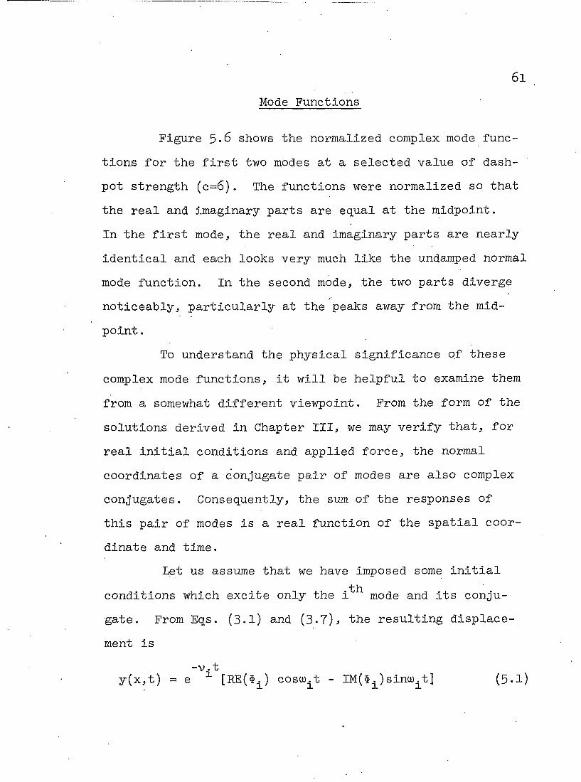
Attenuation and Frequency 53 Mode Functions 6l Comparison with Results by Galerkin's Method 66 Forced Motion Results 70

VI. CONCLUSIONS 74

Methods of Solution 74 Normal Mode Characteristics 75 Concentrated Damping . 76 Suggestions for 'Further Investigation .... 76

v

vi

Page

APPENDIX A SWEEPING MATRICES FOR COMPLEX MODES . . 78

APPENDIX B MATRIX ITERATION PROCESS 82

REFERENCES . 86

LIST OF ILLUSTRATIONS

Figure Page

2.1 General Configuration 9

4.1 Example Configuration . 4l

5.1 Solutions of the Characteristic Equation . 54

5.2 Attenuation for Light Damping 56

5.3 Frequency for Light Damping 58

5.4 Attenuation for a Wide Range of Dashpot Strength 59

5.5 Frequency Variation of the Second Symmetric Mode 60

5.6 Typical Mode Functions for the First Two Symmetric Modes 62

5.7 Effect of Dashpot Strength on the First Mode Function 64

5.8 Effect of. Dashpot Strength on the Second Mode Function 65

5.9 First Mode Attenuation and Frequency Ratios 68

5.10 Attenuation and Frequency Ratios for the Fourth Symmetric Mode 69

5.11 Maximum Strain Energy 71

5.12 Average Power Dissipation 72

vii

ABSTRACT

The primary goal of this investigation was to deter­

mine the effects of concentrated external viscous damping

proportional to transverse velocity on the free and forced

vibration of beams. The model used to represent this

problem was the elementary Bernoulli-Euler differential

equation for flexural vibration, which was modified by add­

ing terms representing the type of damping under considera­

tion.

Starting from this modified equation, general solu­

tions were derived in terms of both exact and approximate

representations of the normal modes of free damped vibra­

tion. Galerkin's method was used to construct the approxi­

mate solution, which may be applied to a wide variety of

beam configurations for which an exact solution is either

impossible or prohibitively difficult. Both general solu­

tions are presented in a form applicable to any beam

configuration' with homogeneous boundary conditions, either

distributed or concentrated damping, and arbitrary forcing

input and initial conditions.

Numerical results for a specific example were cal­

culated from both solutions. The example chosen was a

uniform simply supported beam with a dashpot attached at

viii

ix

the center of its span. Normal mode functions and charac­

teristic frequencies were calculated for a range of dashpot

strength by both methods; comparison showed very good

agreement between exact and approximate values.

Forced vibration due to sinusoidal motion of the

beam supports was considered, and the steady state strain

energy and power dissipated by damping were computed using

the approximate solution.

Results for the example showed that the influence

of concentrated damping may be interpreted in terms of its

effects on the normal modes of vibration. These effects

were found to differ both qualitatively and quantitatively

for the various modes.

The relationship between the normal modes of

damped vibration and their more familiar undamped counter­

parts was examined, and a physically meaningful descrip­

tion of the nature of these modes was offered. Comments

on the utility of the normal mode solutions and suggestions

for further investigation are included.

I. INTRODUCTION

The vibratory behavior of mechanical systems rep­

resented by linear models may be examined in a number of

different ways. Perhaps the most frequently used approach

is the normal mode method in which solutions are con­

structed by summing responses associated with independent

modes of motion. This method has several advantages which

make it particularly attractive for both discrete and con­

tinuous models. First, it leads directly to a set of

uncoupled equations of motion which may be solved by ele­

mentary methods. Second, the normal mode solution facili­

tates physical interpretation of the behavior of the system

in response to forcing inputs. Finally, the response of the

normal coordinates may be found by evaluating convolution

integrals (by numerical methods if necessary); consequently,

the solution for arbitrary inputs is relatively simple.

When viscous damping appears in the model of the

system, the existence of classical normal modes depends on

the distribution of damping in relation to other parameters

of the system. Conditions governing the existence of such

modes are discussed in papers by Caughey and Caughey and

0'Kelly.^ Because a normal mode solution in the usual

1

2

sense is not often available, the analysis of damped

vibrating systems can present formidable difficulty. Under

appropriate conditions, the problem may be circumvented by

using the normal mode functions of the system without damp­

ing to transform the equations of motion into a set coupled

by damping terms alone. If the coupling terms can be

assumed to be sufficiently small, they are neglected, and

the resulting uncoupled equations may be solved to produce

an approximate normal mode solution. The normal mode

approach may be abandoned entirely in favor of an alternate

technique such as the method of mobilities used by Plunk-

11 12 ett. ' Neither of these approaches is entirely satis­

factory. The approximate normal mode solution will not be

adequate for some problems'} while other methods sacrifice

the advantages of the normal mode solution.

Although systems with viscous damping may not

yield to a straightforward application of usual normal

mode techniques, they do possess normal modes in a general

sense. Foss^ has described a modal solution for both free

and forced vibration of damped discrete systems. In addi­

tion, he derived the orthogonality conditions associated

with the integral equation of motion for flexural vibra­

tion- of damped beams. Foss defined a set of velocity

coordinates as the first time derivatives of the existing

generalized coordinates and introduced these velocity

3

coordinates into the second order time derivatives appear­

ing in the equations of motion. Then, the equations which

define the velocity and the equations of motion form a new

set of reduced equations, which contains only first order

time derivatives and possesses an orthogonal mode solution.

Although this approach has the fundamental advantages cited

for normal mode methods, two drawbacks are apparent.

First, reducing the order of the equations doubles the

number of coordinates and increases the complexity of the

solution. The solution could become unmanageable for com­

plicated systems which require a large number of coordinates

to describe their motion. Second, the modes of a damped

system are described by complex vectors for discrete models

and complex functions for continuous models. Consequently,

physical interpretation of the modal solution is not as

convenient as in the case of undamped systems. Perhaps for

these reasons, the method proposed by Foss has been

neglected. Although his paper was published nearly ten

years ago, a diligent search of the subsequent literature

did not turn up a single attempt to use this approach.

Despite the difficulties cited above, the advantages of a

modal solution suggested its use for the problem considered

in this dissertation.

The flexural vibration of damped beams is also a

relatively neglected topic. Cases where classical normal

4

modes exist offer no unusual difficulties and have been

1*3 explored] a paper by Stanek J provides a good example of

this type of problem. Beams with concentrated damping are

interesting from a practical standpoint and have been con-

Q 11 14 sidered by McBride, Plunkett, and Young. None of

these authors developed a complete, solution, but McBride's

results illustrate some significant effects of concentrated

damping. He investigated a uniform cantilever beam with a

dashpot attached to the free end. In this case, damping

enters the problem through boundary conditions, and

McBride was able to develop a closed form solution. A por­

tion of the development of the example to be considered

below follows his approach and yields similar but more com­

plete results.

The basic objective of the study described in this

dissertation is to determine the effects of adding external

damping to a beam as a means of controlling its vibration

response. Particular emphasis is placed on concentrated

damping and periodic input. To achieve this objective, a

solution of the differential equation of motion was needed]

the normal mode approach was selected to provide a solution

of general applicability and hopefully to promote physical

insight.

Exact closed form expressions for the character­

istic frequencies and mode functions of vibrating beams

5

are rarely attainable, even for relatively simple configura­

tions. Effective approximate methods of generating the

mode shapes are essential for normal mode solutions of

practical problems. This observation suggests that a gen­

eral approximate mode solution for the damped case should

be derived. Several techniques are frequently used in

undamped beam problems; one of these, Galerkin's method,

is adaptable to damped systems and quite efficient in terms

of the number of coordinates which must be considered to

obtain good results.

Every investigation needs a starting point. In

this case, it is the familiar Bernoulli-Euler partial dif­

ferential equation modified by adding a term to account for

external viscous damping. This equation is introduced in

the next chapter and further modified to derive the rela­

tions which characterize the complex normal modes.

Galerkin's method is also introduced at this point. The

following chapters contain parallel developments of closed

form and Galerkin's method solutions, first in very general

terms and, subsequently, for a simple example where damp­

ing is concentrated at a point. This example permits an

explicit frequency equation which holds for all levels of

damping however large. The frequency equation and its

associated representation of mode functions are evaluated

numerically to show some of the effects of viscous damping.

6

Corresponding results obtained by Galerkin's method are

compared to the closed form. Finally, the effects of damp­

ing on the forced vibration response of the beam with sinu­

soidal loading are investigated using the Galerkin's method

solution.

II. THEORY

The Equation of Motion

For slender beams, the well-known Bernoulli-Euler

equation is based on the oldest and most often used model

for flexural vibration. The fundamental assumptions on

which this equation rests are as follows:

a. Initially plane cross sections of the beam

remain plane during deformation.

b. The beam is initially straight, and its slope

remains small everywhere along the span during

deformation.

c. The mean axial deflection of any cross section

is zero.

d. Deformation due to shear is neglected.

e. The effect of rotary inertia is neglected.

f. Dissipative effects are not considered.

The derivation of the equation is available in vibration

1 texts, e.g., Anderson, and will not be repeated here.

To account for external viscous damping, the

Bernoulli-Euler equation must be modified. Let us assume

that, in general, the motion of the beam is resisted by a

distributed force with intensity proportional to the

7

8

transverse velocity. This assumption leads to an addi­

tional term,- consisting of the product of the transverse

velocity and a distributed parameter which defines the

force intensity (force per unit length) generated by the

damping mechanism with a unit velocity applied. Point

damping of the beam by one or more isolated dashpots may be

viewed as a special case in which the distributed damping

parameter becomes the sum of a number of terms containing

delta functions.

Figure 2.1 illustrates the general configuration

to be considered. Equation (2.1) is the modified Bernoulli-

Euler equation for this configuration.

% (El^f) +DS + 1J3f|= f (x, T) (2.1) Sx Sx St St

where:

EI = flexural rigidity of the beam

f(x,t) = distributed transverse force applied

L = length of the beam

t~ = time

x = axial beam coordinate

y = transverse deflection of the beam

l_i = mass density (per unit length) of the

beam

D = distributed viscous damping parameter

expressing the ratio of force per unit

9

lxA

IX

s

-ih

O

Fig. 2.1 General Configuration

10

length to unit transverse velocity-

applied to the damping mechanism.

The flexural rigidity, mass density, and damping

parameter vary along the beam. We assume that the beam

may be constrained only at its ends and that the possible

end conditions are limited to the .following cases:

Fixed end -- transverse deflection and slope are zero.

y = 0, = 0 (2.2a) dx

Simply supported end -- transverse deflection and bending

moment are zero.

-s2— y = 0, EI = 0 (2.2b)

dx

Free end — bending moment and shear force are zero.

2 2 EI = 0, (EI -J) = 0 (2.2c)

dx2 Sx Sx2

The results to be developed in subsequent sections

are most conveniently expressed in dimensionless quanti­

ties. To avoid having two complete sets of notation,

Eqs. (2.1) and (2.2) will be written in non-dimensional

form at the beginning, resulting in

- 2 (k -§-) + c IT" + m ~"p" = f(x t) (2-3) dx2 3x2 dt Bt2

11

and end conditions

y = °, || = 0 (2.4a)

~s 2 y = 0, k = 0 (2.4b)

dx

k § - ° ' t y - ° ( s - ^ )

The dimensionless quantities in Eqs. (2.3) and (2.4)-are

defined as follows.

L2 D c =

A,Vo f = L3?

" Vo

k = f-r- (2.5) o o

m =i±-"o

t

* = !

y = 4

EqIo and (i are reference values of flexural rigidity and

mass density taken at a selected location along the beam.

12

For a uniform beam

k(x) = m(x) = 1, 0 < x < 1

Dashpots applied at one or more discrete points along the

beam may be represented by writing D(x) in terms of delta

functions. For M dashpots

_ M _ _ D(x) = S D 6(x - x )

r=l

In non-dimensional form

• M c(x) = Z c 6(x - x )

r=l r

c -Vet: r ""!] I Ll o oHo

(2 .6 )

Normal mode solutions of Eq. (2.3) may be developed

in a straightforward manner if we first transform this

equation into two equations of the first order in time.

m - ** - 0

(k + c + m = f(x,t) (2.7) ox ox

The first equation is an identity used to define

the velocity, vj the second is the equation of motion

reduced to the first order in time.

Orthogonality Conditions

13

Before attempting to construct a modal solution of

Eqs. (2.7)* let us determine the orthogonality conditions

which may be used to obtain uncoupled equations. We begin

with the homogeneous equations obtained from Eqs. (2.7) by

setting the forcing function f equal to zero and assuming

a solution in the form

00 a. t y(x,t) = E a. $,(x) e

i=l x 1

°° ai^ v(x,t) = £ a. \]/. (x) e

i=l 1 1

(2.8)

The i^h terms of Eqs. (2.8) represent the activity in the

*fch i normal mode. When the beam is disturbed by some ini­

tial conditions, the subsequent vibration in any of the

normal modes takes place independently of the activity in

any other mode. Consequently, the i^^1 terms of Eqs. (2.8)

must satisfy both the homogeneous equations and the bound­

ary conditions. Substituting these terms into Eqs. (2.4)

and (2.7) and setting f = 0 leads to

ma. $. - mil;. =0 1 1 Y i

(2-9) tl

(k§^ ) -f ouc$^ -f ct^mij/^ =0

14

and

i $±= 0, $± = 0 (2.10a)

tt = 0, k$± = 0 (2.10b)

tt it I k§± = 0, (k$± ) = 0 (2.10c)

The primes indicate differentiation with respect to x.

Now, let us multiply the first of Eqs. (2.9) "by f . dx, the J

second by $ . dx, sum the two, and integrate over the length J

of the beam.

1 a± J [m($ii)r . + 1 -:) + dx

o (2.11)

1 tt "

+ J C(ki . ) $ . - rm|r A .] dx = 0

o

Since all the normal modes must satisfy Eqs. (2.9), we may

construct another equation from Eq. (2.11) by interchanging

the subscripts i and . Then, subtracting this equation

from Eq. (2.11) gives

1

(ai"aj) J [mU.i. + !);•$,) +c$.l.] dx q J -L J J

1 ». (2-12) + J* [(k^") - (k§j-") dx = 0

o

The symmetry of.- the second integral suggests the next step,

integrating by parts to evaluate this term. Two cases must

15

be considered. In the first case, damping is distributed,

and the shear force is a continuous function of x every­

where along the beam. The second case arises when concen­

trated damping is applied by dashpots attached to the beam.

With concentrated damping, the shear force will have a

step discontinuity at each dashpot. In both cases, the

beam properties and applied force are assumed to be dis­

tributed.

With distributed damping, the second term of Eq.

(2.12) may be integrated twice by parts to obtain

1 " " J [(k$± ) - (kSj ) $±] dx

0

1 I! II It II = J* (k^ § . - k$ . ) dx (2.13)

o

it i it t » i ii i + C (k$± ) ]

The integral on the right side of Eq. (2.13) vanishes

identically, and the integrated terms are zero when the mode

functions satisfy any of the end conditions given by Eqs.

(2.10). If, as is usually the case, the normal modes have

distinct characteristic values, i.e., a.^oc., Eq. (2.12) -L J

reduces to

1 J* j dx = 0

° (2.14) i * 3

16

Taking Eq. (2.14) into Eq. (2.11) produces a second rela­

tion, after integrating by parts.

J (k$± - m^tj) dx = 0, i £ j (2.15)

o

Equations (2.14) and (2.15) are the orthogonality conditions

for the beam with distributed damping.

When the damping is applied through isolated dash-

pots, shear discontinuities exist at the point where the ii i

dashpots act; therefore, (k§^ ) is discontinuous at these

points. If we express the damping function, c, in terms

of delta functions as suggested earlier, Eq. (2.6), the

integrals containing c in Eqs. (2.11) and (2.12) may be

replaced by finite sums.

1 M l J* dx = 2 cr f 5(x-xr) $iij. dx

o r=1 o

M

= Vi <xr) (xr> (2*l6)

From the second of Eqs. (2.9) and Eq. (2.6), the elastic

force term may be expressed as follows.

it " tt " M

(k$± ) = (k0i ) - cu S^cr6(x-xr) $±(xr) (2.17)

it (k0^ )' is continuous. The first two integrals of Eq.

(2.17) are

17 ii 1 it 1 M

(k$± ) = (kOj. ) - a± 2 cr H(x-xr) $±(xr) r=l

II n M ki± = k0± - a± S c (x-xr) H(x-x ) (x.^)

r=l

where H(x-xr) is the unit step function. Eq. (2.17) and its

integrals may be used to evaluate the second integral in

Eq. (2.12). We consider the first term.

1 M "|_ It

J (ki±") = J (Ke±") jjdx O O .

M 1 - a± ^ J1 6(x-xr) §jdx

r o

II " M = J" ) #.,ta - a± 2 =r»1(xr)lJ(xr o

If we integrate by parts twice and use Eq. (2.17) and its

integrals to replace terms involving 0^, we have the same

expression which would result if the shear force were con­

tinuous .

II I

!jdx_= -a -i - a-L -L II 11 + f k$. I. dx J i 0 o o

J,.(k$i") §jdx = [(kS^') ^.-k^V^]

o

For homogeneous end conditions, Eqs. (2.10)/ the integrated

terms are zero; and only the symmetric integral remains on

the right side. Again the second integral in Eq. (2.12) is

zero and the orthogonality conditions are Eqs. (2.14) and

18

(2.15). Equation (2.14) may be modified using Eq. (2.16).

1 M J m($j.<l'j. + ly dx + £ crli(xr)$j(xr = 0 1 (2-19) o r_1

In some cases, the problem of a beam with concen­

trated damping may be solved by considering the undamped

equations of motion on intervals between the dashpots.

The constants in the solutions over these restricted inter­

vals are determined by the end conditions and special con­

ditions which connect the intervals. These special condi­

tions enforce continuity of transverse deflection, slope,

and bending moment across the interval boundaries and equate

the damping force generated by each dashpot to the step in

shear force at its point of application. This approach

will be illustrated in detail in the example given later.

.In this case, the orthogonality conditions may be written

in terms of the sums of integrals taken over the individual

intervals. To write the resulting orthogonality conditions

in compact form, we introduce the notation, repre­

senting the i^h mode function of the interval, <.x _< xr,

where xQ = 0, xM+1 = 1.

19

• Then,

M+l xr M S f m(§.i!f.-fi]f.§.)dx-J-I! c § . (x ) $ . (x ) = 0 v riYrj vrj riy r riv r' rjv r'

x r - l r ~ ±

M+l xr ii ii

r=l (k*rl ?rj " mtri*rj )dx = 0

r-1

i t j

Galerkin's Method

When exact solutions for the vibratory response of

a continuous system are not accessible, we may seek an

approximate solution in terms of a finite number of coor­

dinates. To be useful, an approximate method should pro­

vide solutions which converge on the exact solution as the

number of coordinates is increased. Obviously we would

like to minimize the number of coordinates needed to

reduce the error to an acceptable level. Since Galerkin's

method is quite efficient in this respect, it has been

adopted for the problem being considered here.

Galerkin's method is based on an error weighting

procedure. An approximate solution is constructed from a

set of assumed mode functions (approximating functions)

and an associated set of generalized coordinates. The form

of the solutionis illustrated by Eqs. (2.21). An

(2.20)

20 r

approximate solution in a finite number of coordinates will

not identically sati-sfy the exact equation of motion. The

error, weighted by each of the approximating functions, in

turn, is integrated over the length of the beam, and each

of the resulting expressions is set equal to zero. Prom a

slightly different viewpoint, we may say that the error

is required to be orthogonal to each of the approximating

functions.. Enforcing these conditions produces a set of

ordinary differential equations in the generalized coor­

dinates. The mechanics of the method are illustrated

belowj its mathematical foundations have been described in

10 2 detail by Mikhlin. Bolotin and Kantorovich and

o Krylov have applied the method to a number of interesting

problems.

We begin by assuming that y and v may be expressed

in the following forms.

n y = E cp. (x)q. (t)

i=l 1 1

(2.21)

v = I cp. (x)r. (t) i=l

The approximating functions, cp^(x), are elements of a com­

plete set of functions which satisfy all the boundary condi­

tions- of the system. The functions, and r^(t), are

the generalized coordinates. Anderson"1" suggests that the

approximating functions need only satisfy geometric boundary

• 21

conditions. In this development, however, we will con­

sider only functions which satisfy all the boundary condi­

tions .

Let us substitute Eqs. (2.21) into Eqs. (2.7).

Then,

n . n E mcp.q. - E mcp.r. = D(x,t) i=l 1 1 i=l 1 1

n it " n n E (kcp. ) q. + E ccp.q. + E mcp.r. (2.22) i=l 1 1 i=l 1 1 i=l 1 1

- f(x,t) = E(x,t)

The superscript dots denote differentiation with

respect to time. Since the first of Eqs. (2.7) is an

identity defining velocity, D will be identically zero. To

obtain equations in a convenient form, we will treat D

formally in the same manner as the distributed force error

E which arises from the equation of motion. So, we enforce

the following conditions.

11 J Dp .dx = J Ecp .dx =0

o o (2.23)

j = 1, 2, . . . , nj t > 0.

With these conditions, the work done by the force error

22

will be zero during any displacement which can be expressed

by Eqs. (2.21). Equations (2.23) lead directly to a set

of 2n ordinary differential, equations, Eq. (2.24), written

in matrix form.

(2.24)

[C], [K], and [M] are n x n matrices, and {f} is a 1 x n

matrix.

Their elements are given by

1 Cij = / ccp±cpjdx

o

1 " 1 " Kij = J* ) i^ = «T kcpi dx (2-25)

o o

1 Mij = $ J^PiCPjdx

o

1 FjOO = J f(x^)

o

[C] and [M] are symmetric matricesj and since the

approximating functions obey homogeneous boundary condi­

tions, [K] is also symmetric.

For concentrated damping by N dashpots,

N Cij = Vl^s' "j(Xs)

S=1

23

(2.26)

.5 Equation (2.24) is in the form suggested by Foss-

for lumped parameter systems. He pointed out that a normal

mode solution of this equation is possible if the matrices

are symmetric. We denote the square matrices of Eq. (2.2^1-)

by [D] and [E], respectively.

[D] =

[E] =

0 M

M C

CT

i I o

i

K — —

(2.27)

Then we define

. th {A}± = column matrix form of the i normal mode

vector,

1_A_J^ = Row matrix form of the normal mode «•

vector.

Equations (2.28) are the orthogonality conditions

derived by Poss.

LA4 [D] {A) 3 = 0

La4 [e] [A] . = o

i 3

(2.28)

Some Observations

24

If we can find the normal mode functions and fre­

quencies for a particular beam configuration, the orthog­

onality conditions permit us to construct general solu­

tions for either forced or free damped vibration.' There

are no dependable general techniques which yield exact mode

functions, but we can handle some simple cases.

In Galerkin's method, finding normal mode param­

eters is not so difficult; we may use an iterative process

based on the matrix equation, Eq. (2.24), for this purpose.

The significant problems in this case are selecting good

approximating functions and calculating the elements of the

system matrices.

In any stable linear system with light damping, the

characteristic values will occur in complex conjugate pairs

with negative real parts. The corresponding mode functions

or vectors will also be complex conjugate pairs. The real

part of any of the characteristic values is the subsidence

or attenuation of free damped vibration in the associated

mode; the imaginary part is the corresponding circular fre­

quency. For larger values of damping, some or all of the

circular frequencies vanish; and the free motion of the

corresponding modes changes from decaying oscillation to

exponential decay.

25

The terms, complex frequency and normal mode func­

tion, are not strictly correct when applied to the charac­

teristic parameters of the damped case; eigenvalue and

eigenfunction would be more precise. However, these terms

will be used to emphasize the analogy between the treatment

of damped and undamped problems.

III. GENERAL SOLUTIONS

Closed Form

If we have found normal mode functions, and

frequencies, cu, which satisfy Eqs. (2.9) and applicable

boundary conditions, we may assume the following solution

of Eqs. (2.7).

y= E (x)P. (t)

(3.1) i=l 1 ' 1'

v = E Mx)p. ( t ) i=l 1 1

The first of Eqs. (2.7) determines the form of ty^(x).

^i(x) = ai$i(x)

Substituting Eqs. (3*1) into Eqs. ( 2 . 7 ) , we have

E (m$.p. - ±p±) =0 (3-2) i=l

„ " E C(k§_. ) P. + c$.p. + mtlr.p;,] = f(x,t) i=l ii

Equations (3-2) may be transformed to a set of

uncoupled equations by using the orthogonality conditions.

The first equation is multiplied by .dx, the second by <J

26

27

$.dxj both are integrated over the length of the beam. If J

the resulting equations are summed,

00 . 1 % P± J + c$±$j]dx 1=1 o

00 1 "

+ ^ P± J Ck$j_ ) - milr^jldx (3-3) 1=1 o

1 = J f(x,t)§ .dx

J o

Integrating the terms containing k by parts and

applying the orthogonality conditions, Eqs. (2.14) and

(2.15), the terms where i j drop out. Repeating this

process for all the modes, we have Eqs. (3.4).

RjPj + j-Pj ~ • j = 1, 2, . . ., 00 (3-4)

with ^

R. J* (2m§ 4 . -f c§ . )dx 2

J Q S J T J

" o n I( 2

Sj = J ^dx = J ^dx (3.5)

1 Pj(t) = J <Kf(x,t)dx

We note that R. and S. are the integrals in Eq. (2.11) for J J

the case, i = j.

28

Consequently, we may write

S. = -a.R. j a a

and F . ( t )

Pj~ajpj =-jjr—> J = •••' 00 (3-6) 0

Equations (3-6) may "be solved by elementary means; the com­

plete solution is

a. .t n t a . (t-T) pj^ = pj0 e ° + R7 e 3 Fj(T) dT (3-7)

J o

Pj0 = pj^°)' = 1' 2' * ' "' 00

The initial values, p.(0), may be determined from the ini-

tial displacement and velocity of the beam by setting"

t = 0 in Eqs. (3-1). If we multiply y(x,0) by (m\Jf . + c§ .) J J

dx and v(x,0) by m$..dx, sum and integrate the result over J

the beam length, we have

1 J [(mt . + c§.)-y(x,0) + m$ .v(x,0)]dx

J J J o

00 1

= Z Pi(°) J + + c?i$j.]dx 1=1 o

Applying the orthogonality condition, Eq. (2.l4), only the

"fcfr j term remains on the right side. We may solve for

p.(0) and apply the first of Eqs. (3-5) to obtain 0

j = 1, 2 • • • 9 CO

Finally, the results from Eqs. (3.7) may be substituted

into Eqs. (3-1) to give the displacement and velocity

response of the beam for the initial conditions and applied

forces.

When the damping is concentrated, it may be conven­

ient to represent the mode functions by separate express­

ions for each of the intervals between dashpots. Then,

Eqs. (3.1) may be written for each interval and substi­

tuted into the corresponding differential equations for

that interval. Following the steps outlined for distrib­

uted damping and using the orthogonality conditions, Eqs.

(2.20), instead of Eqs. (2.14) and (2.15), Eq. (3-7) again

gives the solution. In this case, R^, F. and have

the forms shown in Eqs. (3-9).

M-KL xr M M 2

M+l Xr En-(t) = 2 J $ .f(x,t)dx d r=l x , d

30

, M+l Xr pj0 = IT * ^ ml4rj.y(x,0) + $rj.v(x,0)]dx

0 -v-r-1

' M

+ r : S ° r i r j ( x r ) y ( x r ' ° ) ( 3 " 9 )

j r J.

. Galerkin's Method

As pointed out earlier, the frequencies and normal

mode vectors needed.to solve Eq. (2.24) may be obtained "by

an iterative process. Substituting Eqs. (2.27) into Eq.

(2.24) and setting the applied forces to zero, we have

CD] I-4 + [EyfEA = to) (3.10)

q .

We assume

. , 2n an "t = £ {A}± e

For the terms of this series to represent the contribution

of normal modes, each term must satisfy Eq. (3.10).

a.t Q.t a± [D] {A}± e 1 + [E] {A}± e 1 = {0} (3.11)

We may rearrange this equation to obtain Eq. (3-12).

{A}, = -[E]"1 [D] {A}. (3.12) l

31

If we select an arbitrary trial vector and premultiply it

by -[E]"1 [D] a number of times, the resulting vectors

converge to a function of the pair of complex conjugate fre­

quencies having the smallest modulus, together with the

corresponding pair of mode vectors. Fox^ and Frazer, Duncan,

and Collar^ explain this iterative technique and describe

procedures for finding the mode parameters.

Once the lowest modes are determined, we may force

the iteration process to produce the next larger pair of

frequencies and the associated vectors. Appendix A

describes a sweeping matrix technique which accomplishes

this task. We may continue this process until we have

established the required number of modes.

The solution of Eq. (2.24) may now be written in

terms of normal coordinates, Q, .

-4 = [A] {Q} (3-13) <11

The columns of [A] are the normal mode vectors, {A}^. We

substitute this solution into Eq. (2.24) and premultiply

the equation by the transpose of [A].

[A]T[D] [A] {Q} + [A]T[E] [A] {Q} = [A]T j-5-j

The orthogonality conditions, Eqs. (2.28), show that

[A]T[D] [A] and [A]T[E] [A] are diagonal matrices; from

Eq. (3.11)j their diagonal elements are related by

32

LAJ± [D] {A}± = - 1_A_] ± [E] {A}± 1

Consequently, Eq. (2.24) is transformed into a set of 2n

uncoupled equations in the normal coordinates.

-a

± % - 1: LAJ 1 jpj

Ri = LAJ i [DJ i (3.14)

i = 1, 2j 2n

The complete solution of Eqs. (3.14) is:

a.t , t a. (t-T) l_0 Q.(t) = Q.0 e 1 +^- J e 1 ( UJ i]p"f )dT (3'15)

o

i = 1, 2, ..., 2n

with

Q._ = initial values of the normal coordinates. i0

The initial values are derived from the initial displace­

ment and velocity, yo(x) and vo(x)*

From Eqs. (2.21),

n

y°(X) = i=l

n

V°<X) = 1=1

33

We form the functions Z. and Z . and apply Eqs. (2.25), J XiT"J

which define [M] and [C].

Z . J

1 n J mcpjypdx = E MJ;Lq10 (3.16)

n Zn+j = J" (MPjVo+ctPjyoJdx =

o i=l Oi

j — 1 * 2, . . •, n

in matrix form, using the first of Eqs. (2.27)

r. {Z} =

" 0 1 M — <

M _

C _

= [D] [A] CQq} (3.17)

{Z} is a 2n x 1 matrix whose elements are defined by Eq.

(3.16). Premultiplying Eq. (3.17) "by [A]T and applying

the first orthogonality condition from Eqs. (2.28), we may

solve for the initial values of the normal coordinates.

^10 - IT La4 tz} (3-18)

Taking Eqs. (3-15) and (3-18) together gives the

complete solution for the normal coordinates, Q^. To find

the velocity and displacement of the beam in terms of the

normal coordinates, Eq. (3.13) may be substituted into Eqs.

(2.21) after rewriting the latter equations in matrix form.

The result is given by Eqs. (3.19).

34

2x1 2x2n 2nx2N 2Nxl

0 I 0

0 A (3.19)

The number of rows and columns of each matrix are

noted above it. |jp(x)J is a 1 by n row matrix function of

x whose elements are the approximating functions. We have

considered the first N pairs of modes in constructing the

solution. In general, we will wish to supply more approxi­

mating functions than the number of pairs of modes needed.

arbitrary forcing inputs. Among the inputs which may be

considered, those which are periodic in time often occur

in practice. We will examine the behavior of the beam

under this type of loading by inserting a sinusoidal forc­

ing function, Eq. (3.20) into the Galerkin's method solu­

tion.

Harmonic Input

The solutions we have derived permit us to handle

f(x,t) = g(x) sinClt (3 .20)

From the definition of F.(t), Eqs. (2.25), J

1 Fj(t) = sinQt J g(x)cp .dx = h. sinQt

o

where

35

1 hj = J* g(x)cpjdx (3.21)

0 ~ lj 2, ' • ' j n

In matrix form,

0 1 10 sinQt (3.22)

F I I h

Substituting Eq. (3.22) into Eq. (3.15) gives

cut , I 0 I t a. (t-T) qi(t) = qi0e 1 +r7 uji<—> i e sinOTdT

^ I ^ ' o

We may evaluate the integral by elementary means,

+• (^""-^) T OC.t P e sinQTdT = p 9 [a.sinQt + QcosQt-Qe ] J a. -kl 1 o 1

Since the mode frequencies have negative real parts, the

terms containing the exponential will be negligible after

some time. Dropping these terms, we have the steady state

response.

I 0 I a.sinQt + QcosQt «i(t) = - DUi {—} -i—r-S—t, (3*23) 1 W %(«! + 0 )

In matrix form,

{Q} = - [G][A]T sinQt - [H][A]T i cosQt (3-24)

[G] and [H] are diagonal matrices.

Gi± -

Hn =

' a. 1

Rl'(al2-K»2)

n 2,«2N• R^cu^-fT)

Substituting Eq. (3.24) into Eq. (3.19)>

36

(3.25)

v_

y

T'n ~

° lcpTJ

0 I T . i cp J

CA] [G] [A] T J 0.

h

IT J 0

sinfit (3.26)

[A] [H] [A] <---> cosQt

Measures of Damping Effectiveness

The primary goal of investigating structural vibra­

tion is often to assess the possibility that the structure

will fail under the expected vibratory input. "When we are %

free to choose design parameters over a wide range, we may

wish to use strain energy as an initial indicator of the

internal loads within the structure. When viscous damping

is used to control vibratory response, the rate at which

energy must be dissipated by the damping elements is also

important. We may easily derive expressions for strain

energy and dissipation rate from the approximate solution.

37

tion.

by

Consider a "beam undergoing purely flexural deforma-

Its strain energy is given in nondimensional form

U = J -|k(y")2dx (3.27)

o

We may relate this to the energy in appropriate dimensional

units, U, using the definitions of Eqs. • (2.5).

U = ° U

Differentiating.the first of Eqs. (2.21) twice with respect

to x, we obtain y".

n ii y"(x,t) = 2 cp. q.

i=l

substituting this expression into Eq. (3-27), and using Eqs

(2.25)

1 II II

= \ ,4 = i S K^q . n n

U

In matrix form,

u = | LqJ [K] {q}

\ IAJ [a^t _ _ 0 _ _ 0 _

0 K [A]{Q} (3-28)

38

Finally, for the steady state response to the sinusoidal

input of Eq. (3.20), we substitute Eq. (3-24) into Eq.

(3 -28 ) ,

U = -g-(U^sin^Qt -J- 2U2sinfit cosQt + U^cos^fit)

% = L0|hj [A][G][A]T "o lo-1 —t — o JK_,

[A][G][A]T^--h

Vr, = Lojhj [A][G] [A]T ojo7

|k_j

[A][H][A] T J O ,

h (3.29)

U3 =Lo|hJ [A][H][A}T ^o Jo-1

j- - -

_0|K [A] [H] [A] T J 0

h

In nondimensional form, the rate at which work is

done "by the damping force is

• —i-¥ = J* (-cv)vdx (3-30)

Using Eqs. (2.5), this may be transformed to the rate in

dimensional units, ¥.

EI T T 0 0 ¥ = — ¥

Substituting the second of Eqs. (2.21) into Eq. (3-30),

n n 1 ¥ = - E E r.r. J ccp.cp.dx =

• '") js "i * J i=l J=1

n n -EE C .r.r.

i=l J=1 1 D

39

in matrix form

W = - LQj [A] C|0_

o !o [A] {Q} (3.31)

For harmonic input, we may substitute Eq. (3.24) into Eq.

(3-31).

¥ = -

wi -

W2 =

w3 =

2 ? (W-^sin Qt-f2W2 sinfit cosfit + W^cos fit)

j_0;hj [A] [G] [A]

LOjhJ [A] [G] [A]

T

T

L.0jhj [A] [H] [A]T

oj 0_J

r3cj_o_

o! o

"cl o --i— oi o

[A][G][A]

[A] [H] [A]

[A][H][A]

T J_0_

1 h

T J 0_

I h

T J O .

I h

(3.32)

Equations (3-28) and (3*32) show that the strain

energy and energy dissipation rate are periodic functions

of time after transient effects disappear. In general, we

will be most interested in the maximum strain energy and

the average power dissipation. We may write the following

expressions for these quantities.

"max " |(W V4U22 + (U3-Ul>2 >

T . 0 P— = J" Wdt : T =

(3.33)

av T o fi

Then,

Pav " 2 < W (3.34)

IV. APPLICATION TO A SELECTED EXAMPLE

Description of the Problem

We will consider a uniform, simply supported beam

with a single dashpot attached at the center of its span.

Vibration of the beam is forced by sinusoidal translation

of the supports without rocking. The configuration is'

illustrated in Fig. 4.1.

This example is simple enough to permit an exact'

solution for mode frequencies and functions; however, it

exhibits the effects of concentrated damping as well as a

more complicated case would. We will use both exact and

approximate methods to find the normal mode parameters,

but solutions for strain energy and average'dissipated

power will be obtained by Galerkin's method alone. The

exact result would not be substantially better but would

require considerable additional labor.

Before writing the equation of motion, the forcing

input should be defined more precisely. We have assumed

that the support motion is sinusoidal given by

Y(x,t) = YQSinQt

40

4i

T

-j

—Icvi

IX A I 4—

-«J £>

r-hO

+ Q

O < l>%

->»

Fig. 4.1 Example Configuration

42

If we assume that the beam deflection is measured with

respect to the support, the inertia term of Eq. (2.1)

becomes

-s 2 >,2- __2 V —p (y+Y) = ^("Zjp ~ Q YnsinQt)

We return the differential equation to the form of Eq. (2.1)

by defining f(x,t) as follows.

"f = \i YpYgSinQt" (^»1)

To put Eq. (4.1) in nondimensional form, we observe that

the argument of the sine function must be dimensionless.

Then,'using Eqs. (2.5)* we have

n = = "VS- l2" (4-2) O O

and

^ _ mQ Yq (4.3) L

To simplify the following analysis, we will assume the mag­

nitude of Yq is such that the coefficient in Eq. (4.3) is

equal to one.

With the foregoing assumptions, the nondimensional

equation of motion, Eq. (2.3), for the beam illustrated in

Fig. 4.1 becomes

4 2 + c,6(x-i) = sinfit (4.4)

dx^" -1- ^ az bt*

The reduced form corresponding to Eqs. (2.7) is

43

I f - ' - 0

(4 .5)

r~f + p 6 (x~|) If + If = slnt2t OX

The boundary conditions for simply supported ends, Eq.

(2.4b), become

y = ~p" = 0, x = 0, 1 (4.6) dx

Closed Form Solution for Free Vibration

We define the deflection by two functions, one for

the portion of the beam to the left of the dashpot and one

to the right. Each function obeys a differential equation

without damping included, Eqs. (4.7).

•v4 >2 o yn o yn i —rr=- -i J5— = sinfit, 0 < x < -K-

St2 (4-7)

>4 ^2 o yP o yP i —-J- —7=r- ~ sinQt, < x < 1 dx4 St2 2

We may connect the resulting simple solutions through

appropriate continuity and shear conditions at the dashpot

location, Eqs. (4.8) and (4.9). The first equation

expresses continuity of displacement, slope and moment;

44

the second relates the jump in shear to the concentrated

force exerted by the dashpot.

Continuity

2 2 oy-, oyP 3 y-, a yP

*i - y2 - sr - ^ - sjr = °'

x = I (4.8)

Shear

d y-, S y Syx

—t-= cx = 2 ax3 dx3 dt 2

For convenience we have dropped the subscript from c.

We consider the homogeneous form of Eqs. (4.7) and

assume the deflection functions are given in a normal mode

series.

oo a.. t yl = .S *li(x) e 1 ' 0 - x - t

1=1 (4.10)

00 Ct . t -| y2 = $21^ e 1 > 2 - x - 1

The normal mode parameters must each satisfy ordinary dif­

ferential equations of the following form; the mode sub­

scripts will be dropped for clarity.

d\ 2

dx4 + *1 ~ ° (4.11)

a *2 +'cc2|0 = 0 T^f-dx

45

The continuity and shear conditions are

*1 (|) - *2 = 0

" »2'(|) =o

" i2"(|) =0

§i«'(|) . cqSl(l) . i2»(|.) = 0 (4.12)

The solution of Eqs. (4.11) is easily found. After

applying the "boundary conditions at x = 0,lj we have

= A1 sin 2px 4- sinh 2px

= A2 sin 2p(l-x) -f B2 sinh 2p(l-x) (4.13)

a = 'l (2p)2, = V^T

Substituting Eqs. (4.13) into Eqs. (4.12) produces a set

of four homogeneous algebraic equations in four undeter­

mined constants.

In matrix form,

sing -sinp sinhp

cosp cosp coshp

sinp sinp sinhp

G —cos (3 H

-sinhp

coshp

-sinh [3

coshp

= {0}

(4.14)

46

where A T C1

G = -cosp - ~ sinp

X\ H = coshp - sirihp

We must now seek the values of a which permit non-zero

constants. Accordingly, we require that the determinant of

the matrix in Eq. (4.14) be zero. Expanding that determi­

nant leads directly to the characteristic equation.

/x sinp sirihp[|p-(sinhp cosp - sinp coshp)

- 8 cosp coshp] = 0 (4.15)

Before examining the implications of Eq. (4.15)>

let us define real variables representing the real and

imaginary parts of a and p.

a = - v + iou

p = a •+ ib

(4.16)

We will call v the attenuation and uu the circular frequency,

They are related to a and b by Eq. (4.17).

v = 8ab (4.17)

uj = 4(a2 - b2)

47

Equation (4.15) will be satisfied if either

sinp sinhp = 0 (4.18)

or

c = - 8$fe cosg coshg

(4.19) sinhpcosp - sinpcoshp

Equation (4.18) leads to purely real or imaginary values of

P. Then, either of the following occurs.

These cases yield the antisymmetric modes of the undamped

beam; each of these modes has a node at midspan. and is

therefore not affected by the dashpot. Since the assumed

load does not excite the antisymmetric modes, we will

neglect them.

solving Eq. (4.19). The limiting cases are zero and infin­

ite damping. In both cases, p is again either real or

imaginary; the symmetric modes are respectively those of

the undamped simple beam and an undamped beam on three

equally spaced supports.

or

2 a = 0, b = nir, v = 0, ID = - (2mr)

n = 1,2,3, • •

The symmetric modes of the beam are established by

48

For finite, non-zero values, of c, the right-hand

side of Eq. (4.19) is a complex function. Since c is real,

admissible values of p are those which make the imaginary

part of this function zero. Then, the real part gives the

corresponding value of c. We expand the equation in terms

of a and b and set the imaginary part equal to zero. Equa­

tions (4.20) define c.

G(a,b) = (cosh 2b -f cos 2a)(b sin 2a - a sin 2b)

4-(cosh 2a + cos 2b) (a sin 2a - b sin 2a)

(4.20) H(a,b) = cosh 2a cosh 2b - cos 2a cos 2b •

- sin 2a sinh 2a - sin 2b sinh 2b

The parts of p must satisfy

(cosh 2a + cos 2b)(asin 2a + bsinh 2b) (4.21)

• - (cosh 2b + cos 2a)(bsin 2b + asinh 2a) = 0

After Eqs. (4.20) and (4.21) are solved by some

means, we may determine the mode parameters by substituting

the solutions (a,b) into Eqs. (4.13) and (4.l6). The con­

stants in Eqs. (4.13) are determined by Eq. (4.l4). We

may express the other three constants in terms of and

49

arbitrarily make = 1; the mode functions are defined by

the following.

cos[3 . *1± = sin2p.x - sinhSp.x

cosp'. $2i = sin2Pi(1-x) - coshg^ sinh2pi(l-x) (4.22)

B . = a. + b. pi l i

Equation (4.21) must be solved by numerical means.

If we survey a range of values for a and b and calculate

the function on the left-hand side, we may estimate the

loci by noting where the sign changes. Examining the forms

of Eqs. (4.20) and (4.21) will be helpful. If (a^,b^) is

a solution of these equations, (b^a^), (-a^,-b^), and

(-b.,-a.) are also solutions for the same c. If we take v 2.' l' each of these solutions into Eqs. (4.17) and (4.22), we

observe that the second solution yields mode frequencies

and functions which are complex conjugates of those given

by the first solution. The third and fourth solutions

repeat the results of the first two with only the sign of

the mode functions changed. Finally, if a^ and b^ have

opposite signs, the attenuation would be negative, implying

unstable free-vibration which is not possible for the

assumed model. Consequently, solutions of Eqs. (4.20) and

(4.21) for values of a and b lying in the region bounded by

the positive a axis and the line, a=b, determine all the

50

physically possible sets of mode parameters. The line,

a=b, is itself a solution of Eq. (4.21). In this case,

the circular frequency is zero; and the solution repre­

sents heavy damping in the fundamental mode. For this

solution, Eq. (4.20) reduces to

= 8a coshga + oosSa (4_23) sinh2a - sin2a v '

Galerkin's Method

The first and most important task is to select an

appropriate set of approximating functions. After this is

done, the rest of the solution proceeds in a straight­

forward and orderly manner.

For the problem considered here, we will use the

mode functions of the equivalent undamped beam. This

choice is attractive for several reasons. These functions

satisfy the boundary conditions and are simple in form.

The necessary matrices will be diagonal, which is certainly

convenient. Accordingly, the approximating functions are:

cpi(x) = sin(ifrx)

This set includes the antisymmetric modes; in the

previous section we remarked that they were unaffected by

either the damping or the loading assumed here. Conse­

quently, we consider only the symmetric functions.

51

cp, (x) = sin(m.Trx) ' 1 1 (4.24)

= 2i - 1

We proceed directly to determine the elements of

the system matrices using the definitions of Eqs. (2.25)>

(2.26), and (3-21).

m.TT m.Tr . . Cij' = Cji = c sin(-g-)sin -g-) = (-1) (-l)Jc

M. . = M.. = f sin(m.Trx) sin(m .irx)dx = -is. . J1 J 1 J ^ iJ

K^. = Kji = J (miTr)lt"sin(mi7rx)sin(mj7rx)dx = j

o

1 1 h . = J sin(m .7rx)dx = - —: [cos (m .it)-1] = j J v J m.Tr J m.Tr

o

6,, = < (4-25) J 1,1=3

Finally, in explicit matrix form,

52

[C] = c

1 - 1 1 -1 1 -1 1 - 1 1

[M] = \

1 0. , . .0 0 1.. . .0

0 • • 1 0. . . .1

= ki]

[K]

10 0. . 0 4 o 810.

• • 0 TT 2

• •

•

• o o .m 4

(4.26)

ih} i tr

The equation of motion becomes

+ -M' 0 -~1— 0| M

I -1

y q

sinQt (4.27)

With these matrices determined, we may calculate

the mode vectors and frequencies for various values of c

by the iterative process based on Eq. (3-12). The steady

state solutions for displacement, strain energy, or power

dissipation are.easily obtained from the equations pre­

sented in Chapter III.

V. NUMERICAL RESULTS

Attenuation and Frequency

The characteristic equation, Eq. (4.15)\> was solved

by assuming values of a and increasing b in steps until the

sign of the left side of the equation changed. The esti­

mates of b were improved by reducing the step size and

examining the interval between the last two estimates. The

process was repeated over successively smaller intervals

until it reached two values of b which surrounded the solu­

tion and differed by less than .001$. Figure 5-1 shows

some of the solutions of Eq. (4.15).

As the dashpot strength goes up, the curves repre­

senting the first symmetric mode intersect the line, a=b.

At this intersection, the first mode is critically dampedj

its free vibration passes from a decaying oscillation to

exponential decay. The corresponding dimensionless value

of the dashpot strength is : cs«9 • 59 •

As damping increases beyond this value, the first

mode solution has two branches which follow the line, a=b.

One branch moves from the intersection toward the originj

the second moves outward from the intersection.

53

MODE 2

oo > 0

MODE I

MODE 2 MODE 3

5.0 7.5 2.5

Fig. 5»1 Solutions of the Characteristic Equation

Arrows indicate the direction of the solution as. damping increases.

55

The other modes are not critically dampedj their

free vibration will be oscillatory for any level of dash-

pot strength. As Fig. 5*1 shows, their solutions finally

return to the a and b axes. In contrast to this situation,

if the damping is distributed along the entire length of

the beam, all the modes become critically damped at suffi­

ciently high values of the damping parameter. This sug­

gests that to critically damp more of the normal modes,

additional dashpots must be employed.

With the solutions of the frequency equation

established, we may plot the variations in mode parameters

with dashpot strength. Figure 5-2 is a plot of the atten­

uation in the first four symmetric modes for light damping,

i.e., less than the critical value for the first mode. It

is interesting that attenuation in all the modes increases

almost linearly with the damping. We ordinarily expect

free vibration of the higher modes to damp out more rapidly

than that of the fundamental mode. Contrary to this expec­

tation, Fig. 5»2 shows little difference in attenuation

among the four modes at low damping levels. At slightly

higher values of damping, the second mode shows the lowest

attenuation; while the fundamental mode has the highest

attenuation and will consequently damp out more rapidly

than the others.

56

MODE 3 MODE 4>

101 MODE I

MODE 2 81

61

41

4 8 10 6 0 2

Fig. 5.2 Attenuation for Light Damping

57

Figure 5-3 plots the circular frequencies of the

same modes for light damping. Here, the effect of damping

is greater in the first mode, decreasing as the mode

number goes up.

In Fig. and Fig. which extend over a

larger range of damping, we can see how the attenuation and

frequency approach a limiting case where the dashpot begins

to act like a rigid support. Figure 5*^ shows the branching

of the attenuation curves for the lowest modej one branch

approaching zero, the other increasing with the damping.

In contrast, the attenuation for the other modes rises to a

maximum and then gradually drops until it begins to approach

the c axis asymptotically. The peak attenuation and the

value of dashpot strength at which it occurs both increase

as the mode number goes up.

Figure 5*5 shows the variation of circular fre­

quency in the second mode; the curve is also representative

of the higher modes. We notice that the curve takes a

knee shape, which asymptotically approaches the frequency

of the lowest symmetric mode of a beam on three supports

(id = 61.67) .

58

484~ cu

482.

247"

245.

891

MODE 2

86.

10

MODE 1

for Light Damping Fig. 5-3 Frequency

MODE 4

MODE I 40"

MODE 4

MODE 3

MODE 2

MODE I

100 150 50

Pig. 5.^ Attenuation for a Wide Range of Dashpot Strength ui

6o

aj

80"

70""

61.67

100 60 20

Fig. 5-5 Frequency Variation of the Second Sym­metric Mode

Mode Functions

6l

Figure 5-6 shows the normalized complex mode func­

tions for the first two modes at a selected value of dash-

pot strength (c=6). The functions were normalized so that

the real and imaginary parts are equal at the midpoint.

In the first mode, the real and imaginary parts are nearly

identical and each looks very much like the undamped normal

mode function. In the second mode, the two parts diverge

noticeably, particularly at the peaks away from the mid­

point .

To understand the physical significance of these

complex mode functions, it will be helpful to examine them

from a somewhat different viewpoint. From the form of the

solutions derived in Chapter III, we may verify that, for

real initial conditions and applied force, the normal

coordinates of a conjugate pair of modes are also complex

conjugates. Consequently, the sum of the responses of

this pair of modes is a real function of the spatial coor­

dinate and time.

Let us assume that we have imposed some initial

conditions which excite only the i mode and its conju­

gate. From Eqs. (3.1) and (3-7)j the resulting displace­

ment is

- v . t y(x,t) = e [RE($i) cosuut - IM^^)sinuKt] (5-1)

62

IMAGINARY

0.5

2

REAL N\ IMAGINARY

Fig. 5^6 Typical Mode Functions for the First Two Symmetric Modes

63

For simplicity, we have absorbed the initial values of the

normal coordinates into the mode functions. Since the

relative values of real and imaginary parts of the mode

function vary along the beam, we conclude that the phase of

the resulting vibration varies with x. Let us write $j_(x)

in the form,

$±(x) = * ± ( x ) [cos0^(x) -f'l sin0^(x)]

Putting this into Eq. {^.1), the displacement becomes

-v. t y(x,t) = * ± ( x ) e 1 cos[uut + 0^(x)] (5*2)

From a physical standpoint, the interesting prop­

erties of a complex mode function are its magnitude, which

describes the amplitude of the motion at each point along

the beam, and its argument, which indicates the phase lead

angle at each point. In Figs. 5-7 and 5*8* the magnitude

and phase angle of the first two modes are plotted for sev­

eral values of light damping. The curves have been normal­

ized so that the magnitude is one and the phase angle is

zero at midspan.

From Fig. 5-7* we see that the first mode function

changes very little under light damping. The change in

phase for this mode is quite small. For the highest value

of dashpot strength shown (c=9)> the phase angle curve

falls below the. intermediate curve (c=5)• This'suggests

64

0 . 5 .

0 . 0 1.0 0.5

c«9

0.5 1.0

Fig. 5.7 Effect of Dashpot Strength on the First Mode Function

65

0 . 5 .

0.0 1.0 0.5

180.

c=9

9 0 .

0 0.5 1.0

Fig. 5-8 Effect of Dashpot Strength on the Second Mode Function

66

.that at critical damping, the first mode function is again

real as in the undamped case. Examining Eqs. (4.22) for

the case, a = b, it is possible to verify that the normal­

ized mode function is real for any damping at or above the

critical value.

In Pig. 5-8* the effect of damping on the second

mode function is most noticeable near the nodes of the

undamped mode. With damping, the nodes disappear; and as

the dashpot strength goes up, the displacement near these

points also grows. At other points along the beam, the

magnitude of the function is not greatly affected by the

damping. The changes in phase angle are rather straight­

forward. As damping is increased, the phase curves depart

further from the undamped case, for which each point of

the beam moves either in phase or 180 degrees out of phase

with respect to the reference point.

Comparison with Results by G-alerkin's Method

Complex frequencies and mode functions obtained by

Galerkin's method agreed very closely with the exact result

Values for the first four modes at selected dashpot

strengths were determined by matrix iteration, using (in

turn) the first 4, 5* 6, and 7 approximating functions.

Appendix B describes the mechanics of the iteration process

67

To compare attenuation and circular frequency cal­

culated at both methods, the ratios of values determined

by Galerkin's method to the corresponding exact parameters

were plotted as functions of dashpot strength. Figure 5-9

and Fig. 5>10 show comparisons of parameters of the first

and fourth modes for light damping-and several choices of

n, the number of approximating functions used.

We observe that the solutions for successive val­

ues of n tend to converge as n goes up. This convergence

is an important characteristic of Galerkin's method, which

permits us to estimate the number of approximating functions

needed. If we construct a sequence of solutions for increas­

ing n and continue until the difference between two succes­

sive solutions is negligible, the convergence property

suggests that increasing n further will not significantly

affect the result.

In Fig. 5 - 9 > the circular frequency ratios increase

sharply near critical damping. The reason for this

increase is not certain; however, the first mode frequency

is approaching zero in this region, and the relative effect

of small differences may be exaggerated by taking the

ratios.

Using the mode functions of the undamped beam in

the Galerkin's method solution, we would expect agreement

with the exact solution to be best for small damping and to

68

^ APPROX.

EXACT

1.000

n=4

n = 4

CO APPROX.

^EXACT

1.002-

1.001-

1.000

Fig» 5-9 First Mode Attenuation and Frequency-Ratios

69

APPROX.

EXACT

1.000

0.990-

co APPROX.

^ EXACT

1.000

0.999-

Fig. 5.10 Attenuation and Frequency Ratios for the Fourth Symmetric Mode

70

deteriorate as dashpot strength goes up. The curves shown

in Figs. 5-9 and 5.10 support this assumption and also

indicate that using a greater number of approximating func­

tions both improves the agreement and reduces its variation

with damping level.

Since the sine functions used here cannot exactly

account for the shear discontinuity at the dashpot, con­

vergence of the approximate solution will become rather

poor as damping is increased. To improve the convergence

under these conditions, we may include an additional

approximating function for which the associated shear func­

tion has a step discontinuity. A suitable choice would be

the static deflection curve of the beam with a concentrated i

force applied at the location of the damper.

Forced Motion Results

Maximum strain energy and average power dissipa­

tion for a range of input frequencies were calculated using

Eqs. (3-33) and (3-3^). Figure 5.11 and Fig. 5-12 show

curves of these quantities for several values of dashpot

strength. In Fig. 5-llj strain energy curves for the

undamped beam and the beam on three supports have been added

for comparison. In both sets of curves, the acceleration

amplitude of the support motion is assumed to be the same

-I '1 10 'J

I0"2-J

I0"3d

IO"4-rj

c = 00

(RIGID SUPPORT)

10" ~r~ 20

c = 0 ,1

T~ 40

—r" 60

I 80

sl t -

Fig. 5»11 Maximum Strain Energy

ro"'"d + P.

AVE

ld2d

IO"°-d

I04d

10% 20

~1 40

~I— 60

Fig. 5.12 Average Power Dissipation

~I— 80

n .

-si ro

73

for any input frequency. Other input limitations could be

considered without serious difficulty using the same gen­

eral equations.

Figure 5-H shows clearly that the sensitivity of

the strain energy to changes in the dashpot strength

depends strongly on the input frequency. If we wished to

control the response of the beam by adding concentrated

damping, our strategy and chances of success will be influ­

enced by the frequency characteristics of the input. For

example, in a relatively low frequency range, we may sup­

press the strain energy most effectively by replacing the

dashpot with a rigid support.

The variation of power dissipation with damping

also depends on input frequency. Obviously, the power must

be zero for the limiting cases and have a maximum for some

intermediate value of damping. The curves show that the

maxima near the resonance peaks are greater and occur at

smaller values of dashpot strength than at other values of

input frequency.

For this steady state solution, the power dissipa­

tion curve also represents the power being supplied at the

support to produce the displacement input.

VI. CONCLUSIONS

Methods of Solution

Exact and approximate normal mode solutions for the

flexural vibrations of damped beams have been shown. The

exact solution is possible in some cases, but it is not

very convenient. Even in the rather simple problem consid­

ered here, deriving the exact frequency equation required

a great deal of tedious algebra.

The approximate solution by Galerkin's method

yielded quite accurate results with a relatively small

amount of labor. This approach may be applied in a straight­

forward and orderly manner to a wide variety of assumed

damping distributions. The only changes would be in cal­

culating the elements of the damping matrix. For concen­

trated damping, this is particularly easy since the need

for integrating products of several functions is eliminated.

In practical problems, stiffness and inertia dis­

tributions are frequently complicated enough to require

approximate solutions even for undamped problems. If

viscous damping is present in such cases, the approximate

solution derived here is particularly attractive.

74

Normal Mode Characteristics

75

It seems reasonable that complex normal mode solu­

tions for problems with viscous damping may have been

neglected primarily because of two factors. First, the

increase in the number of coordinates and the difficulty of

determining mode functions make this approach appear

extremely complicated. Second, the physical interpretation

of complex mode functions is not so readily apparent as in

the case of the usual real functions.

The first factor becomes less important for many

problems with the use of approximate methods, such as the

one described here, and modern digital computers to carry

out the necessary calculations.

We may clarify the meaning of complex mode func­

tions by considering each pair of complex conjugate modes

as a mathematically convenient representation of the

activity of one physically possible mode of free damped

vibration. In this "physical" mode, each part of the system

executes damped motion with the same attenuation and circu­

lar frequency but, in general, differing phase and ampli­

tude. Systems which may be uncoupled by the classical

normal modes become merely a special case where the phase

of the motion of each point is the same. Undamped beams

are another specialization, characterized by uniform phase

and zero attenuation.

• . 76

Concentrated Damping

The solution of the example considered here

revealed two interesting properties of a beam with concen­

trated viscous damping.

First, for the beam with a simple dashpot, only the

fundamental mode has associated with it a critical level of

damping, above which its characteristic free motion changes

from damped oscillation to exponential decay. Each of the

other modes exhibits oscillatory free motion at all values

of dashpot strength.

Second, even below the critical value of damping,

the fundamental has the highest attenuation of the modes

examined. This implies that the free motion of the funda­

mental will subside before that of the higher modes. This

is at odds with the usual assumption that free vibration of

the higher modes of a beam will damp out most rapidly.

Suggestions for Further Investigation

Any investigation of a relatively neglected topic

is bound to produce more new questions than answersj the

present work is no exception. The most promising questions

stem from the rather interesting consequences of concen­

trated damping described in Chapter V.

The relatively weak effect of a single dashpot on

modes other than the fundamental suggests examining beams

. 77

having several dampers to explore the possibility of achiev­

ing more effective control of beam response. One specific

objective should be to test the conjecture that using addi­

tional dashpots will force more than one mode to exhibit a

critical damping level. The influence of varying the loca­

tions at which concentrated damping elements are attached

to the beam should also be investigated.

Finally, since the suggested investigations of

concentrated damping will depend on efficient approximate

methods, attention should be paid to improving the G-aler-

kin's method solution developed here. For example, con­

vergence at higher damping levels may be slow due to the

relatively large shear discontinuities. It would be useful

to explore ways to improve the convergence under these con­

ditions .

APPENDIX A

SWEEPING MATRICES FOR COMPLEX MODES

The matrix iteration process based on Eq. (3-12)

produces the pair of modes whose frequencies have the low­

est modulus. To find the frequencies and vectors of other

modes, we must suppress the effects of the dominant lower

modes. To do this, we may insert sweeping matrices into

the iteration equation; these matrices receive their name

from the idea that they "sweep" the lower modes out of

the iteration. We will describe a convenient way to con­

struct these matrices for equations with complex normal

mode vectors.

We note that the 2n normal mode vectors are ele­

ments of a 2n dimensional vector space and are linearly

independent. Consequently, they form a basis of the space,

and any vector of that dimension may be expressed as a

linear combination of these mode vectors.

We may express the assumed trial vector used in

the iteration process as follows.

0 2n

{A} = 6± {A^ + E d± {A}±

78

79

We construct the expression,

LAjj [E] [A}° = d1 LAJ2 [E] {A3-L

2n + £ a, _A_n [E] {A},

i—2

Prom the orthogonality conditions, Eqs. (2.28), we see that

the terms of the series on the right side are each zero.

We may solve for the scalar coefficient, d-^.

LAJ1 [E] [A}° d = :

LAJ-l [E] {A}2

We must also remove the complex conjugate mode. We

arrange the sequence of the modes so that the (n-J-i) mode

is the conjugate of the i^h mode*

u3n+1 = 03*

where the asterisk denotes the complex conjugate. We may

write the coefficient, dn+]_«

_ LA4+1 [E] [A}° _ LA4* [E] {A}°

dn+1 " LAJn+1 [E] (A}n+1 = LAJX* [E] {A3l*

Since [E] and {A}0 are real, and are complex con­

jugates .

8o

We may now remove the lowest mode terms from the

trial vector.

{A}° - {A)° - {A}^ - {A}n+1dn+1

= {A}° - CA} 1d1 - {Aj-^dj*

' = {A}° - 2RE [ {A} 1d-L]

If we substitute for d^ and factor the original trial vec­

tor.,

(A}° = [U - 2RE {A} 1 |_AJ. [E]_

LAJ-L [E] {A}1 {A} 0

The square matrix is the sweeping matrix which will remove

the lowest mode components from any real assumed vector.

To use this sweeping matrix, we first define [V^].

[ Y j ] = - [E] _1[D]

Now, we premultiply the swept vector by [V^] and use Eq.

(3.12).

{A}i lAJL [E] [V1] {A)° = [V-lI - 2 RE

ai LAli

{A} (

= [V0] {A} 0

81

If we use [Vgl ^-n iterative process, the lower modes

are swept out at each step. This prevents convergence to

these modes if they are accidentally introduced by the

numerical process.

The same process may be continued until all modes

•of interest are established. In general,

- t V - 2 R E tA}^ LAj-i [B]

. Oj LAJj [E] tA} J_

APPENDIX B

MATRIX ITERATION PROCESS

Normal mode parameters satisfying Eq. (3.12) were

calculated through the iterative technique described by

Pox.6 This appendix will summarize the technique briefly

and describe the criteria used to decide when to termi­

nate the iteration.

To determine the i^h pair of modes, we use the

matrix [V^], defined in Appendix A, and an arbitrary real

trial vector {A}0. We calculate some of the powers of the

iteration matrix and form the following expressions using

three successive powers of [V^],

{zs3 = [vi]s [A}°

{zs+1} = [v±]s+:L [A}° _

{ZS+2} = [V.]3*2 {A}0

We choose two sets of corresponding elements of the result­

ing vectors and solve the following pair of equations for

f and g.

82

83

z s+2 + fZ s+1 + gZ_s = o J J J

Zks+2 + fZkS+1 + gZkS = 0

Then we may estimate the complex frequency,

ai =" (fg)

The elements of the corresponding vector are

J — 1 j •••) 2n

If we calculate f and g for several choices of j

and k, the values obtained will vary somewhat. As s

increases, these values and the resulting estimates of the

mode frequencies and vectors converge.

In calculating normal mode parameters for the prob­

lem considered here, this convergence of results for dis­

tinct choices of j and k was used to indicate when the iter­

ation had been carried far enough. At each step of the

iteration, reference values of f and g calculated from one \

pair of vector element sets were compared with values

84

obtained from other pairs. We identify the reference

values with the subscript r and calculate the following

expression for each of the other results.

/ (f-fr)2 + (S-gr)2

v f 2 + s

2 -r r

When this expression was less than a predetermined value

for each possible choice of vector element sets, the iter­

ation was ended and the mode frequency and vector were cal­

culated. Otherwise, s was increased, and the process

repeated.

In problems where the number of vector elements is

large, this procedure may become rather cumbersome; the

calculation of B must be repeated many times at each step

near the end of the iteration.

The matrix iteration process was carried out on a

Control Data Corporation model 3600 digital computer. For

this problem, the [V^] were 14 by 14 matrices. The

results were first tested at s=4, and s increased by one at

each step until all values of B were sufficiently small.

-5 Several upper limits on B were examined, and 10 was

finally selected to produce the results shown in Chapter V.

This limit was deliberately kept quite small to keep errors

in the lower modes small. Lower mode errors will affect

85

the sweeping matrices and thus produce errors in the higher

modes.

Prom 15 to 35 iterations were required, depending

on which mode was being calculated; higher modes required

fewer iterations. As a check on both the iteration pro­

cess and the sweeping matrices, the estimates of frequen­

cies and mode vectors were inserted into Eq. (3.12). In

each case, the difference between the two sides of the

equation was negligible, occurring usually in the fifth or

sixth significant figure.

Although the iteration process seems rather lengthy,

calculating four sets of modes for each of nine values of

damping required less than three minutes running time on

the computer. This included constructing the iteration

matrices, performing the iteration, calculating sweeping

matrices, and .computing mode functions from the vectors and

original approximating functions.

Mode function data were recorded on magnetic tape

for subsequent automatic plotting. Figures 5*6, 5-7* and

5.8 were produced from these data using a CALCOMP 565 digi­

tal incremental plotter.

REFERENCES

1 Anderson, Roger A., Fundamentals of Vibrations, Macmillan, New York, 1967•

2 Bolotin, V. V., Nonconservative Problems of the Theory of Elastic Stability, Macmillan, New York, 1963•

3 Caughey, T. K., "Classical Normal Modes in Damped Linear Systems," Journal of Applied Mechanics, Vol. 27, Trans. ASME, Vol. 02, Series E, I960, pp. 269-271.

4 Caughey, T. K. and M. E. J. 0'Kelly, "Classical Normal Modes in Damped Linear Dynamic Systems," Journal of Applied Mechanics, Vol. 32, Trans. ASME, Vol. 87* Series E, 1965, pp. 583-588.

5 Foss, K. A., "Coordinates "Which Uncouple the Equations of Motion of Damped Linear Dynamic Systems," Journal of Applied Mechanics, Vol. 25. Trans. ASME, Vol. 80, 1958, PP. 361-364.

6 Fox, L., The Numerical Solution of Two-Point Boundary Problems, Oxford University Press, London, 1957-

7 Frazer, R. A., ¥. J. Duncan, and A. R. Collar, Elementary Matrices, Cambridge University Press, London, 1946, p. 327-

8 Kantorovich, L. V. and V. I. Krylov, Approximate Methods of Higher Analysis, Interscience, New York, 1958, pp. 258-303.

9 McBride, E. J., "The Free Lateral Vibrations of a Cantilever Beam with a Terminal Dashpot," Journal of Applied Mechanics, Vol. 10, Trans. ASME, Vol. 65, 1943, pp. A-168 to A-172.

86

87

10 Mikhlin, S. G., Variational Methods In Mathematical Physics, Macmillan, New York, 1964* PP- 448-490.

11 Plunkett, R., "The Calculation of Optimum Concentrated Damping for Continuous Systems, ' Journal of Applied Mechanics, Vol. 25, Trans. ASME, Vol. 80, ±95°) pp. 219-224.

12 Plunkett, R., "Vibration Response of Linear Damped Complex Systems," Journal of Applied Mechanics, Vol. 30, Trans. ASME, Vol.-85, Series E, 19^3, pp. 70-74.

13 Stanek, Floyd J., "Free and Forced Vibrations of Canti­lever Beams with Viscous Damping," NASA TN D-2831, National Aeronautics and Space Administration, Washington, 1965•

14 Young, Dana, "Vibration of a Beam with Concentrated Mass, Spring, and Dashpot," Journal of Applied Mechanics, Vol. 15* Trans. ASME, Vol. JO, 1948, pp. b5-72.