Embed Size (px)
DESCRIPTION
MELJUN CORTES RESEARCH Lectures Triangulation Research
Citation preview
Data Analysis Basics:Variables and Distribution
Goals Describe the steps of descriptive
data analysis Be able to define variables Understand basic coding principles Learn simple univariate data
analysis
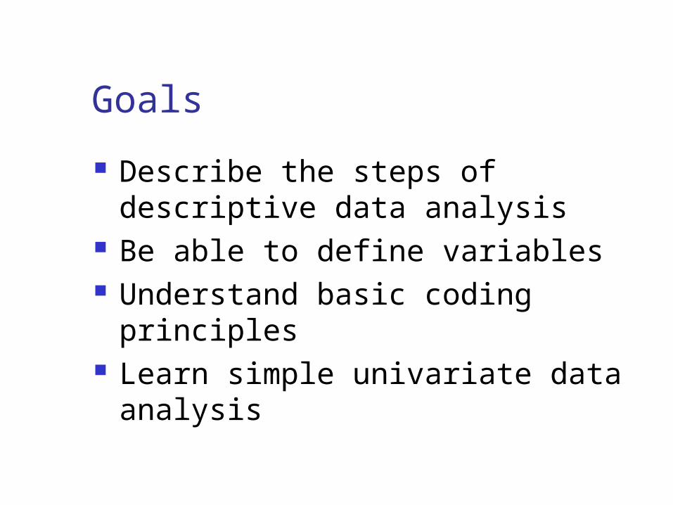
Types of Variables Continuous variables:
Always numeric Can be any number, positive or negative Examples: age in years, weight, blood pressure
readings, temperature, concentrations of pollutants and other measurements
Categorical variables: Information that can be sorted into categories Types of categorical variables – ordinal,
nominal and dichotomous (binary)
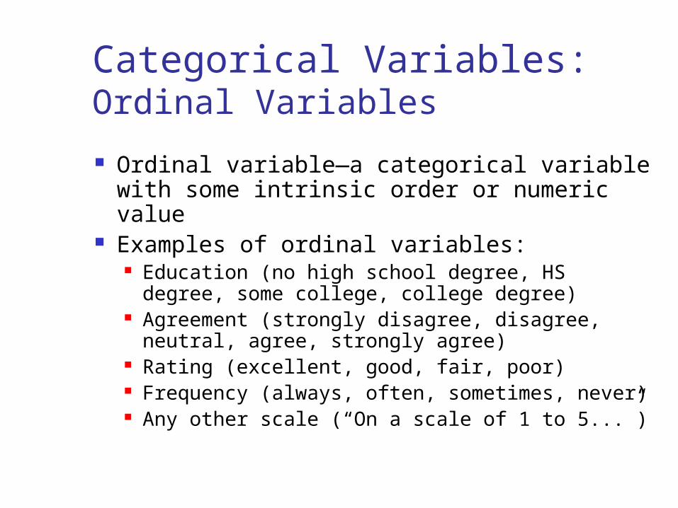
Categorical Variables:Ordinal Variables Ordinal variable—a categorical variable
with some intrinsic order or numeric value Examples of ordinal variables:
Education (no high school degree, HS degree, some college, college degree)
Agreement (strongly disagree, disagree, neutral, agree, strongly agree)
Rating (excellent, good, fair, poor) Frequency (always, often, sometimes, never) Any other scale (“On a scale of 1 to 5...”)
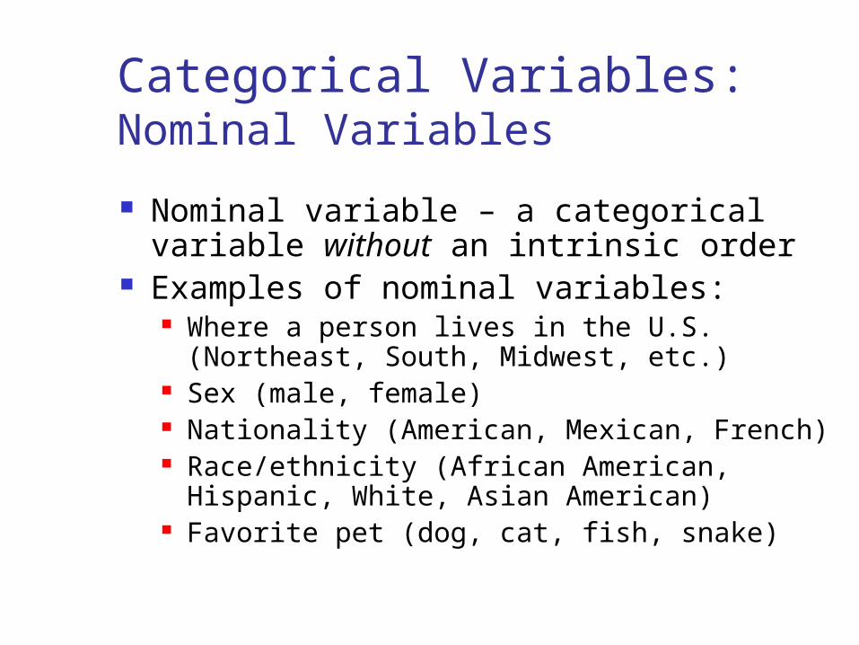
Categorical Variables:Nominal Variables Nominal variable – a categorical
variable without an intrinsic order Examples of nominal variables:
Where a person lives in the U.S. (Northeast, South, Midwest, etc.)
Sex (male, female) Nationality (American, Mexican, French) Race/ethnicity (African American, Hispanic,
White, Asian American) Favorite pet (dog, cat, fish, snake)
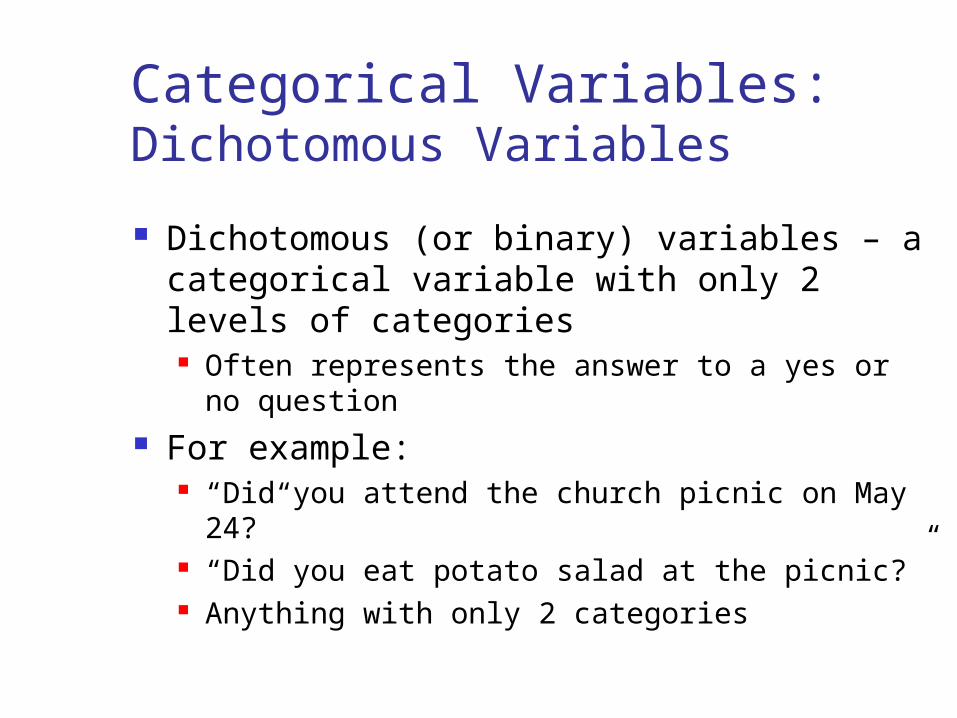
Categorical Variables:Dichotomous Variables Dichotomous (or binary) variables – a
categorical variable with only 2 levels of categories Often represents the answer to a yes or no
question For example:
“Did you attend the church picnic on May 24?” “Did you eat potato salad at the picnic?” Anything with only 2 categories
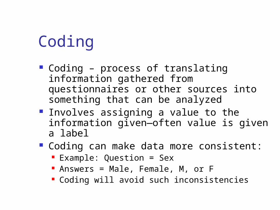
Coding Coding – process of translating information
gathered from questionnaires or other sources into something that can be analyzed
Involves assigning a value to the information given—often value is given a label
Coding can make data more consistent: Example: Question = Sex Answers = Male, Female, M, or F Coding will avoid such inconsistencies
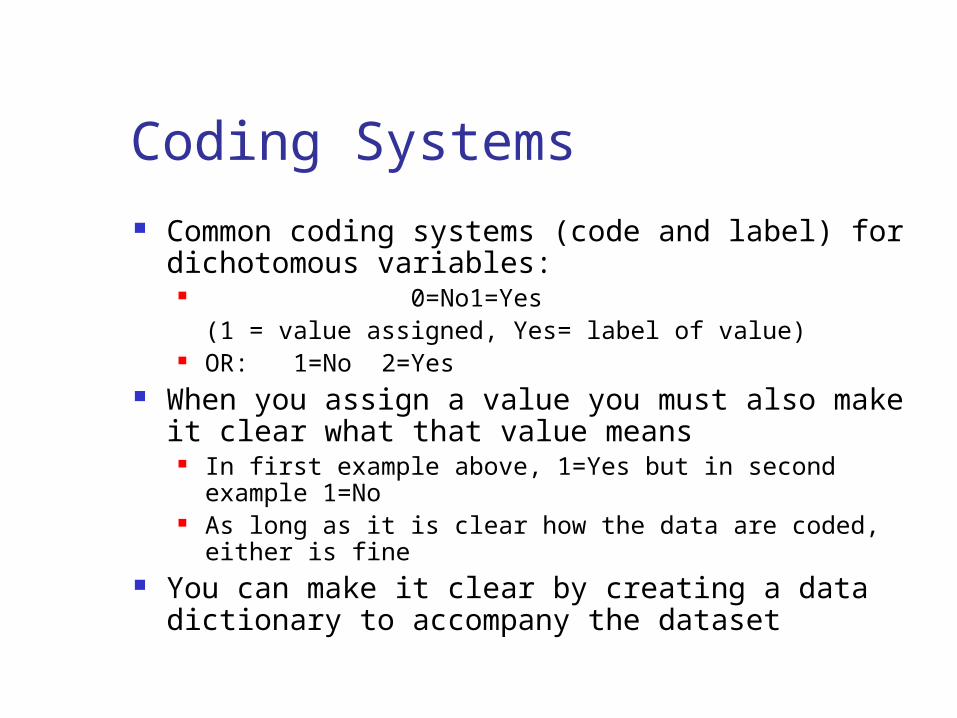
Coding Systems Common coding systems (code and label) for
dichotomous variables: 0=No 1=Yes
(1 = value assigned, Yes= label of value) OR: 1=No 2=Yes
When you assign a value you must also make it clear what that value means
In first example above, 1=Yes but in second example 1=No
As long as it is clear how the data are coded, either is fine You can make it clear by creating a data dictionary
to accompany the dataset
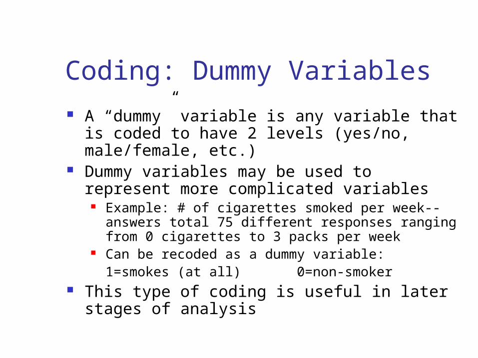
Coding: Dummy Variables A “dummy” variable is any variable that is
coded to have 2 levels (yes/no, male/female, etc.)
Dummy variables may be used to represent more complicated variables
Example: # of cigarettes smoked per week--answers total 75 different responses ranging from 0 cigarettes to 3 packs per week
Can be recoded as a dummy variable:1=smokes (at all) 0=non-smoker
This type of coding is useful in later stages of analysis
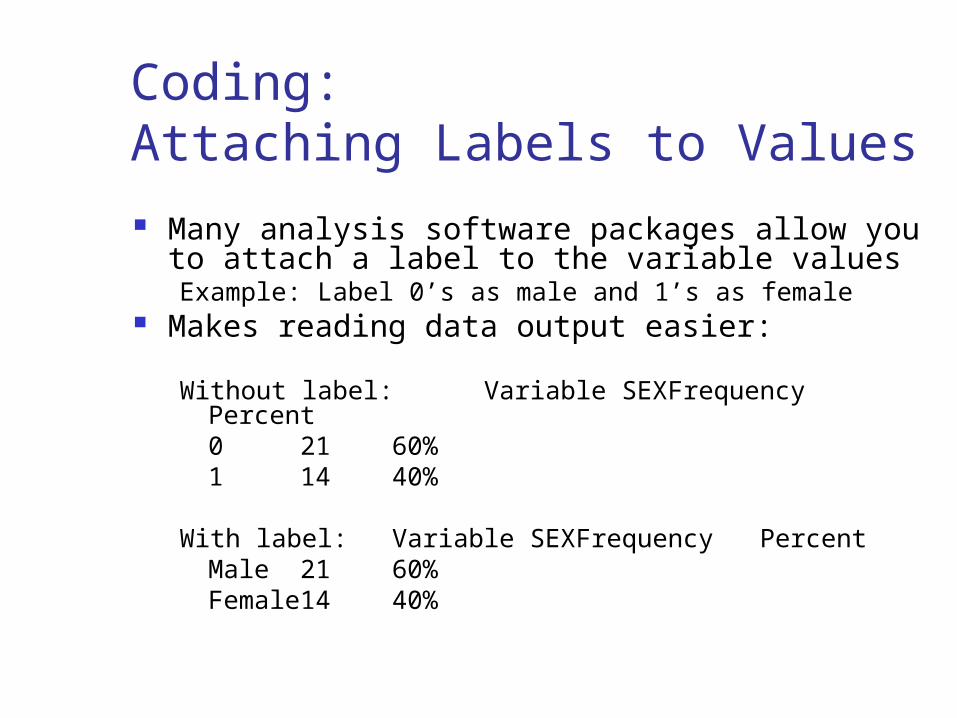
Coding:Attaching Labels to Values Many analysis software packages allow you to
attach a label to the variable valuesExample: Label 0’s as male and 1’s as female
Makes reading data output easier:Without label: Variable SEX Frequency Percent
0 21 60%1 14 40%
With label: Variable SEX Frequency PercentMale 21 60%Female 14 40%
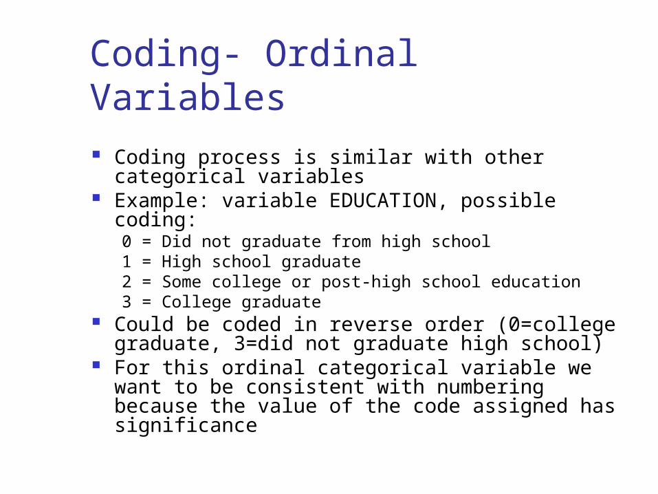
Coding- Ordinal Variables Coding process is similar with other categorical
variables Example: variable EDUCATION, possible coding:
0 = Did not graduate from high school1 = High school graduate2 = Some college or post-high school education3 = College graduate
Could be coded in reverse order (0=college graduate, 3=did not graduate high school)
For this ordinal categorical variable we want to be consistent with numbering because the value of the code assigned has significance
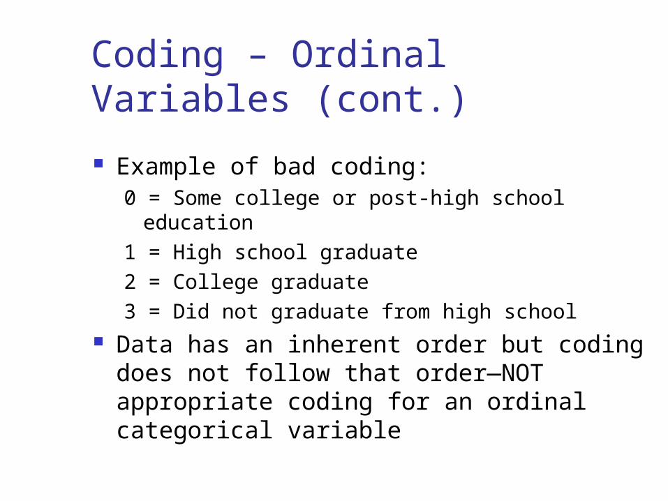
Coding – Ordinal Variables (cont.) Example of bad coding:
0 = Some college or post-high school education1 = High school graduate2 = College graduate3 = Did not graduate from high school
Data has an inherent order but coding does not follow that order—NOT appropriate coding for an ordinal categorical variable
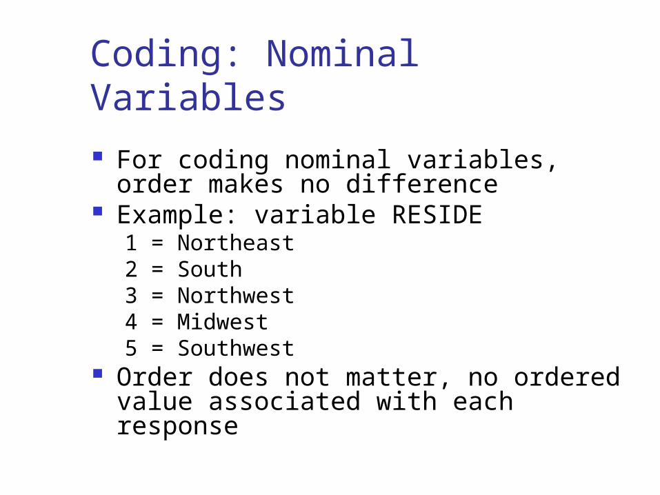
Coding: Nominal Variables For coding nominal variables, order
makes no difference Example: variable RESIDE
1 = Northeast 2 = South 3 = Northwest 4 = Midwest 5 = Southwest
Order does not matter, no ordered value associated with each response
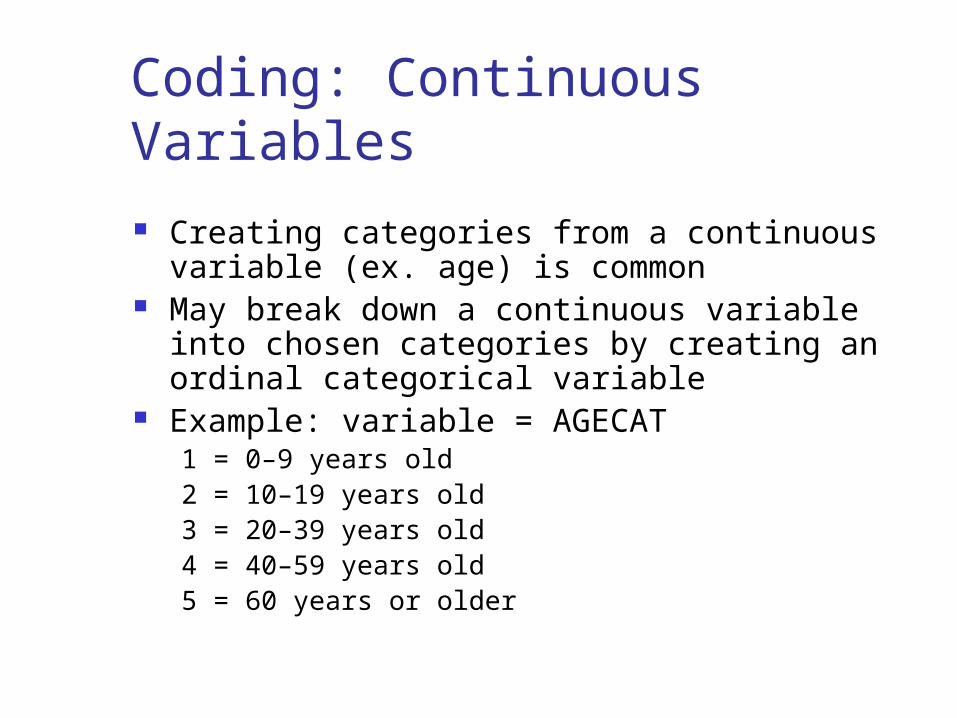
Coding: Continuous Variables Creating categories from a continuous variable
(ex. age) is common May break down a continuous variable into
chosen categories by creating an ordinal categorical variable
Example: variable = AGECAT1 = 0–9 years old2 = 10–19 years old3 = 20–39 years old4 = 40–59 years old5 = 60 years or older
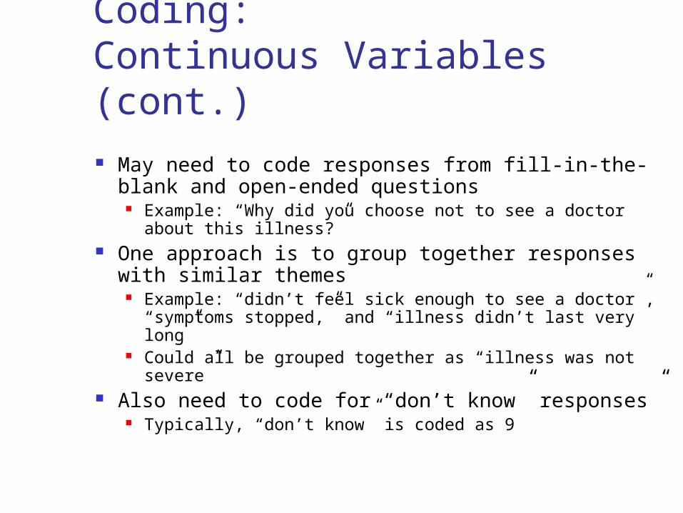
Coding:Continuous Variables (cont.) May need to code responses from fill-in-the-
blank and open-ended questions Example: “Why did you choose not to see a doctor
about this illness?” One approach is to group together responses
with similar themes Example: “didn’t feel sick enough to see a doctor”,
“symptoms stopped,” and “illness didn’t last very long” Could all be grouped together as “illness was not
severe” Also need to code for “don’t know” responses”
Typically, “don’t know” is coded as 9
Coding Tip Though you do not code until the
data is gathered, you should think about how you are going to code while designing your questionnaire, before you gather any data. This will help you to collect the data in a format you can use.
Data Cleaning One of the first steps in analyzing data is to
“clean” it of any obvious data entry errors: Outliers? (really high or low numbers)
Example: Age = 110 (really 10 or 11?) Value entered that doesn’t exist for variable?
Example: 2 entered where 1=male, 0=female Missing values?
Did the person not give an answer? Was answer accidentally not entered into the database?
Data Cleaning (cont.) May be able to set defined limits when entering
data Prevents entering a 2 when only 1, 0, or missing are
acceptable values Limits can be set for continuous and nominal
variables Examples: Only allowing 3 digits for age, limiting words
that can be entered, assigning field types (e.g. formatting dates as mm/dd/yyyy or specifying numeric values or text)
Many data entry systems allow “double-entry” – ie., entering the data twice and then comparing both entries for discrepancies
Univariate data analysis is a useful way to check the quality of the data
Univariate Data Analysis Univariate data analysis-explores each
variable in a data set separately Serves as a good method to check the
quality of the data Inconsistencies or unexpected results
should be investigated using the original data as the reference point
Frequencies can tell you if many study participants share a characteristic of interest (age, gender, etc.) Graphs and tables can be helpful
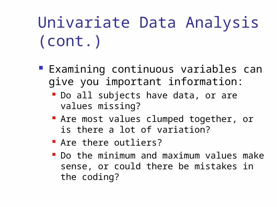
Univariate Data Analysis (cont.) Examining continuous variables can give
you important information: Do all subjects have data, or are values
missing? Are most values clumped together, or is
there a lot of variation? Are there outliers? Do the minimum and maximum values make
sense, or could there be mistakes in the coding?
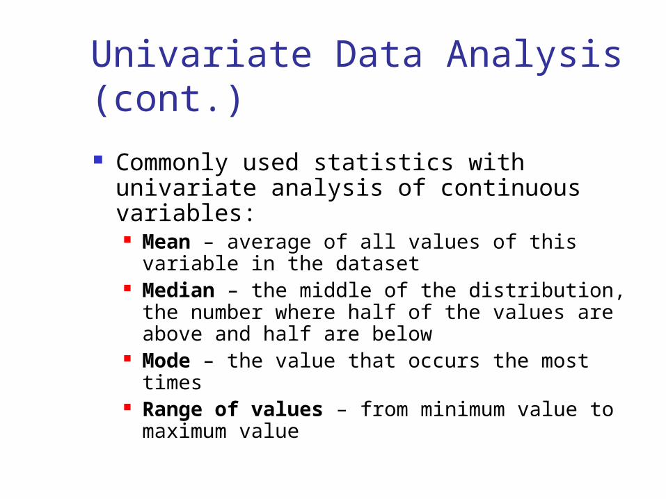
Univariate Data Analysis (cont.) Commonly used statistics with univariate
analysis of continuous variables: Mean – average of all values of this variable in
the dataset Median – the middle of the distribution, the
number where half of the values are above and half are below
Mode – the value that occurs the most times Range of values – from minimum value to
maximum value
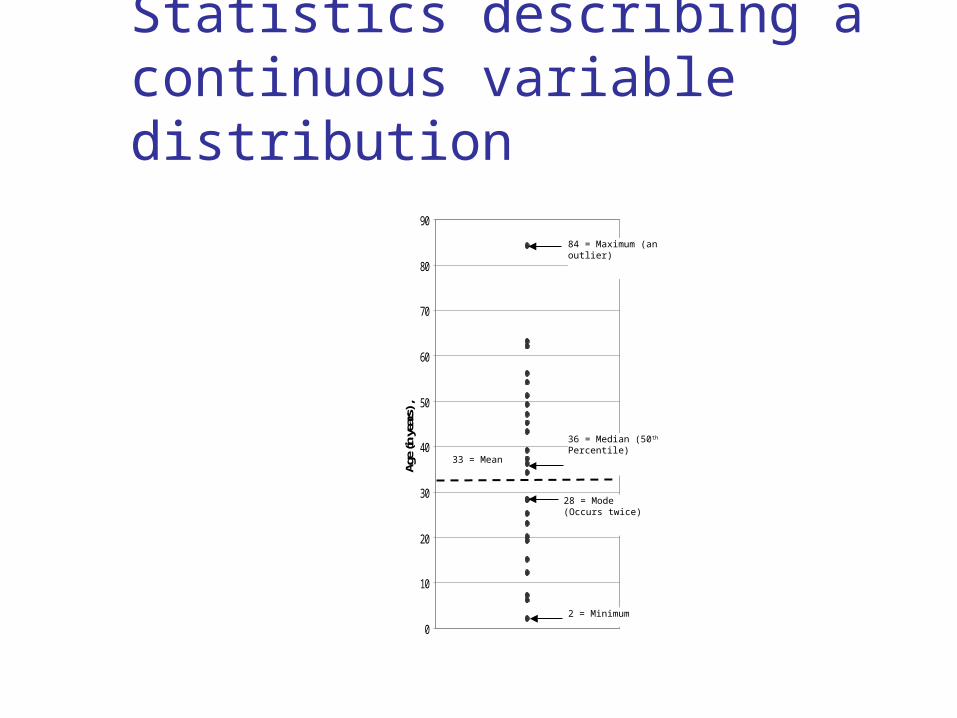
Statistics describing a continuous variable distribution
0
10
20
30
40
50
60
70
80
90
Age (in
yea
rs) ,
84 = Maximum (an outlier)
2 = Minimum
28 = Mode (Occurs twice)
33 = Mean
36 = Median (50th Percentile)
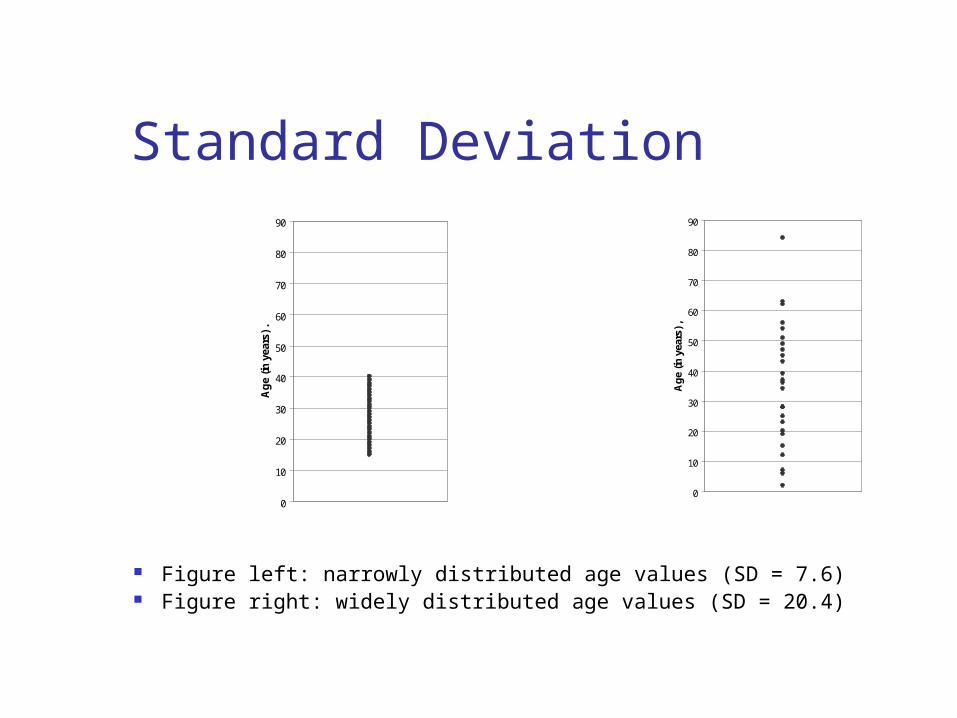
Standard Deviation
0
10
20
30
40
50
60
70
80
90
Age
(in y
ears
) .
0
10
20
30
40
50
60
70
80
90
Age
(in y
ears
) ,
Figure left: narrowly distributed age values (SD = 7.6) Figure right: widely distributed age values (SD = 20.4)
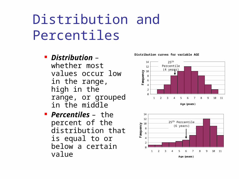
Distribution and Percentiles Distribution –
whether most values occur low in the range, high in the range, or grouped in the middle
Percentiles – the percent of the distribution that is equal to or below a certain value
0
2
4
6
8
10
12
14
1 2 3 4 5 6 7 8 9 10 11
Age (years)
Freq
uenc
y0
2
4
6
8
10
12
14
1 2 3 4 5 6 7 8 9 10 11
Age (years)
Freq
uenc
y
Distribution curves for variable AGE
25th Percentile(4 years)
25th Percentile(6 years)
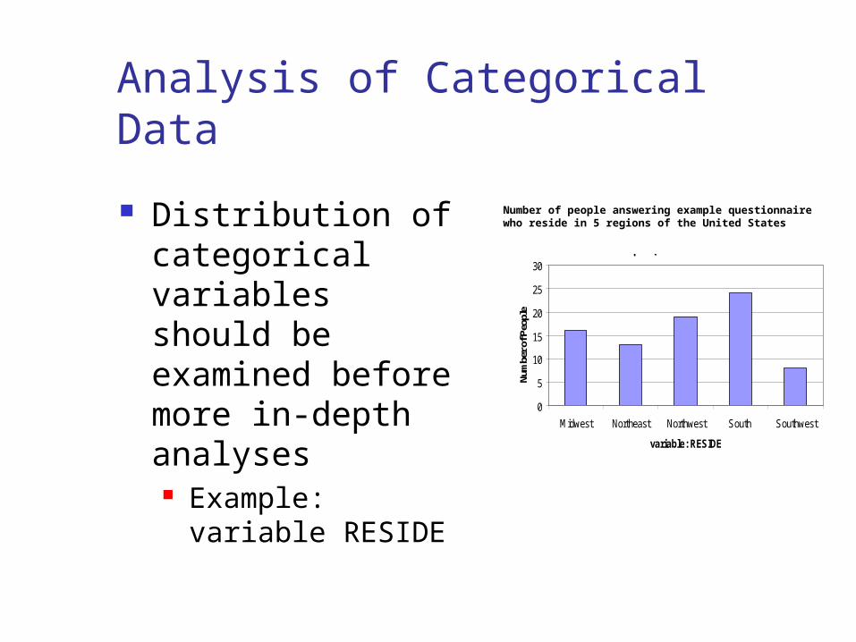
Analysis of Categorical Data Distribution of
categorical variables should be examined before more in-depth analyses Example: variable
RESIDE
Number of people answering example questionnaire who reside in 5 regions of the United States Distribution of Area of Residence
Example Questionnaire Data
0
5
10
15
20
25
30
Midwest Northeast Northwest South Southwest
variable: RESIDE
Num
ber o
f Peo
ple
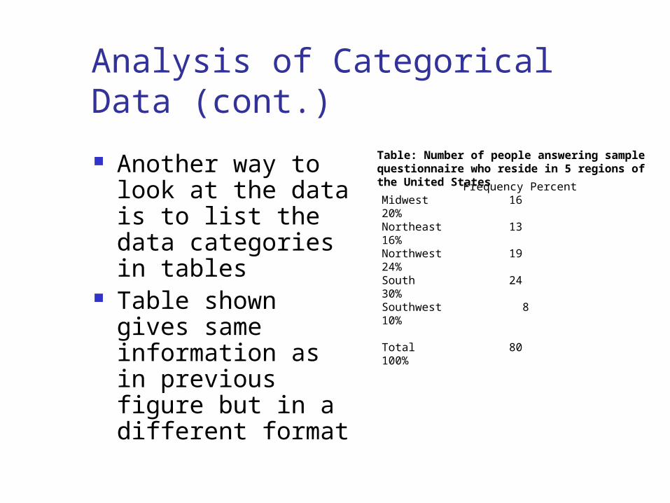
Analysis of Categorical Data (cont.) Another way to
look at the data is to list the data categories in tables
Table shown gives same information as in previous figure but in a different format
Frequency PercentMidwest 16 20%Northeast 13 16%Northwest 19 24%South 24 30%Southwest 8 10%
Total 80 100%
Table: Number of people answering sample questionnaire who reside in 5 regions of the United States
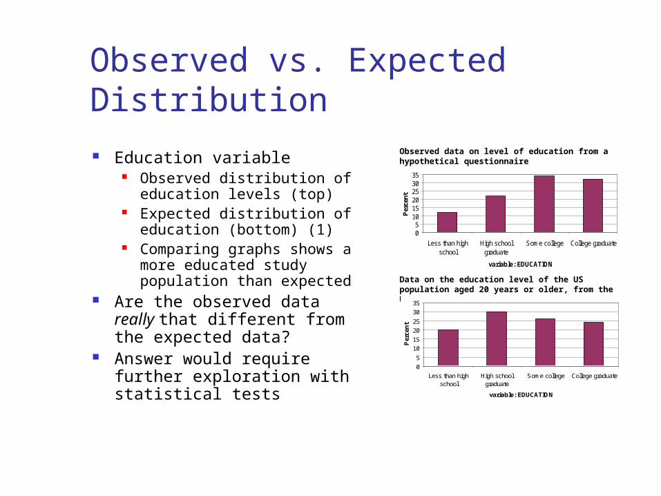
Observed vs. Expected Distribution Education variable
Observed distribution of education levels (top)
Expected distribution of education (bottom) (1)
Comparing graphs shows a more educated study population than expected
Are the observed data really that different from the expected data?
Answer would require further exploration with statistical tests
Observed data on level of education from a hypothetical questionnaire
05
101520253035
Less than highschool
High schoolgraduate
Some college College graduate
variable: EDUCATION
Perc
ent
Data on the education level of the US population aged 20 years or older, from the US Census Bureau
05
101520253035
Less than highschool
High schoolgraduate
Some college College graduate
variable: EDUCATION
Perc
ent
Conclusion Defining variables and basic coding
are basic steps in data analysis Simple univariate analysis may be
used with continuous and categorical variables
Further analysis may require statistical tests such as chi-squares and other more extensive data analysis
References1. US Census Bureau. Educational Attainment in
the United States: 2003---Detailed Tables for Current Population Report, P20-550 (All Races). Available at: http://www.census.gov/population/www/socdemo/education/cps2003.html. Accessed December 11, 2006.