Embed Size (px)
Citation preview
Turin 2021
Mellin amplitudes &
1D CFTs
Gabriel J. S. Bliard Based on work with L. Bianchi, D. Bonomi, V. Forini & G. Peveri
[2106.00689]
also [2004.07849]

G. Bliard Mellin amplitudes & 1d CFTs2
Why do we care?CFT1 theories are omnipresent
• Subsector of higher dimensional theories • Boundary of QFT in AdS2 • Defect theories
AdS2 worldsheet excitations Operator insertions on the Wilson line
Mellin amplitude in higher d
• Nice complex analytic structure • Clear links to scattering amplitudes • Redundant variables for 1d
G. Bliard Mellin amplitudes & 1d CFTs3
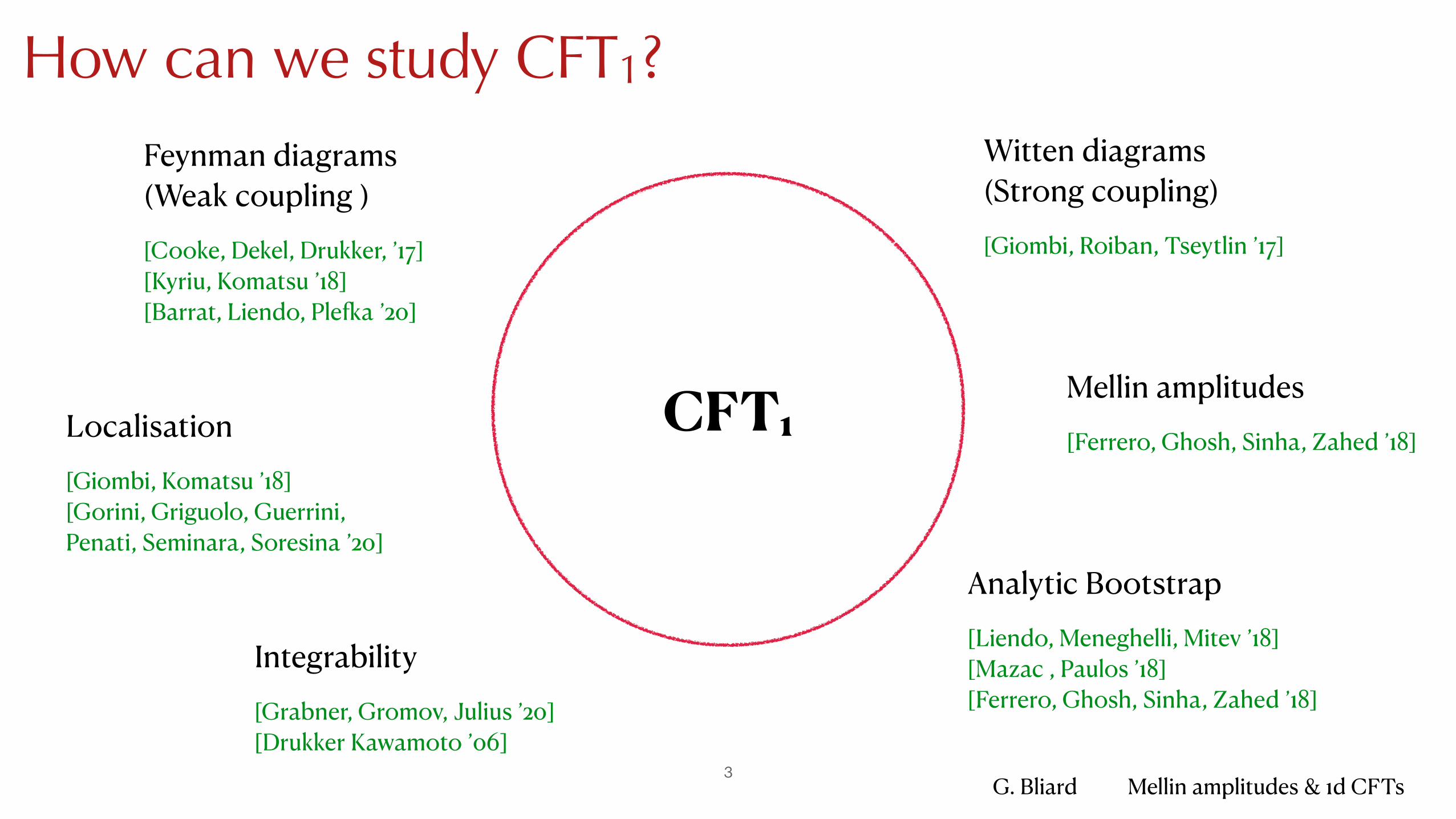
How can we study CFT1?
Localisation [Giombi, Komatsu ’18] [Gorini, Griguolo, Guerrini, Penati, Seminara, Soresina ’20]
Mellin amplitudes [Ferrero, Ghosh, Sinha, Zahed ’18]
Analytic Bootstrap [Liendo, Meneghelli, Mitev ’18] [Mazac , Paulos ’18] [Ferrero, Ghosh, Sinha, Zahed ’18]
Integrability [Grabner, Gromov, Julius ’20] [Drukker Kawamoto ’06]
Feynman diagrams (Weak coupling ) [Cooke, Dekel, Drukker, ’17] [Kyriu, Komatsu ’18] [Barrat, Liendo, Plefka ’20]
Witten diagrams (Strong coupling) [Giombi, Roiban, Tseytlin ’17]
CFT1
G. Bliard Mellin amplitudes & 1d CFTs4
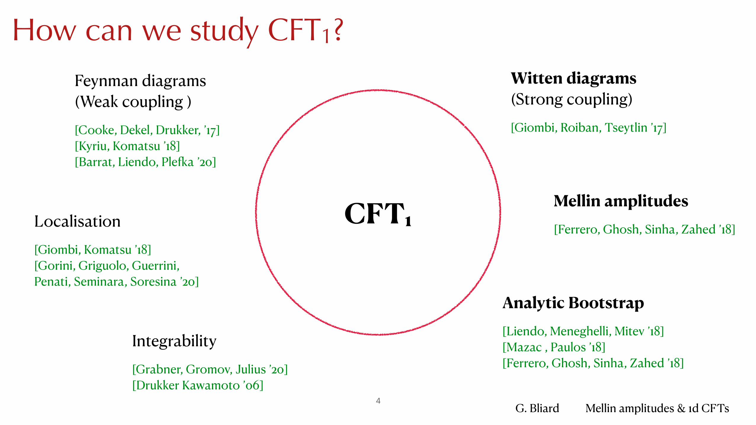
How can we study CFT1?
Localisation [Giombi, Komatsu ’18] [Gorini, Griguolo, Guerrini, Penati, Seminara, Soresina ’20]
Mellin amplitudes [Ferrero, Ghosh, Sinha, Zahed ’18]
Analytic Bootstrap [Liendo, Meneghelli, Mitev ’18] [Mazac , Paulos ’18] [Ferrero, Ghosh, Sinha, Zahed ’18]
Integrability [Grabner, Gromov, Julius ’20] [Drukker Kawamoto ’06]
Feynman diagrams (Weak coupling ) [Cooke, Dekel, Drukker, ’17] [Kyriu, Komatsu ’18] [Barrat, Liendo, Plefka ’20]
Witten diagrams (Strong coupling) [Giombi, Roiban, Tseytlin ’17]
CFT1
G. Bliard Mellin amplitudes & 1d CFTs5
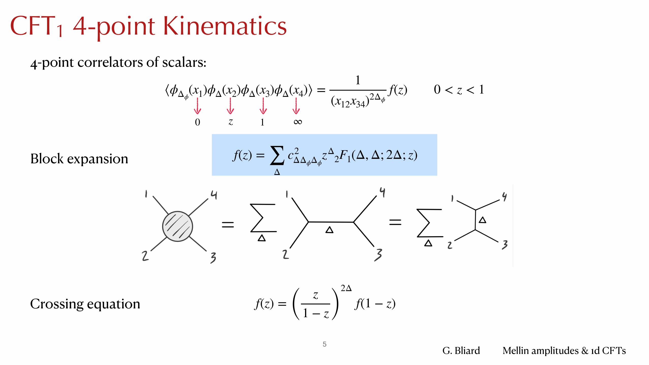
CFT1 4-point Kinematics4-point correlators of scalars:
⟨ϕΔϕ(x1)ϕΔ(x2)ϕΔ(x3)ϕΔ(x4)⟩ =
1(x12x34)2Δϕ
f(z) 0 < z < 1
Block expansion
0 z 1 ∞
f(z) = ( z1 − z )
2Δ
f(1 − z)Crossing equation
f(z) = ∑Δ
c2ΔΔϕΔϕ
zΔ2F1(Δ, Δ; 2Δ; z)
G. Bliard Mellin amplitudes & 1d CFTs
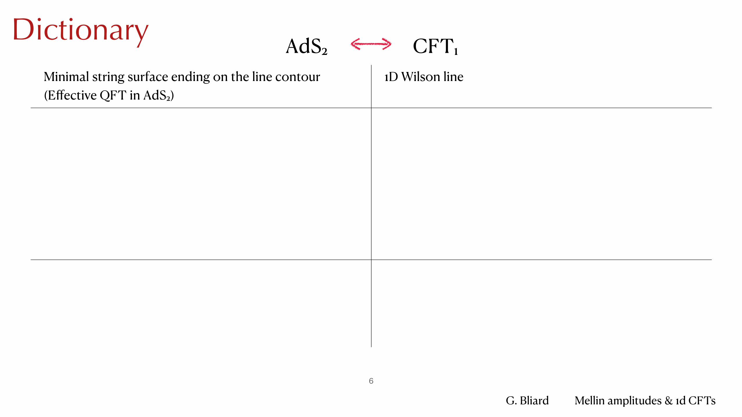
Minimal string surface ending on the line contour (Effective QFT in AdS2)
1D Wilson line
6
AdS2 CFT1 Dictionary
G. Bliard Mellin amplitudes & 1d CFTs
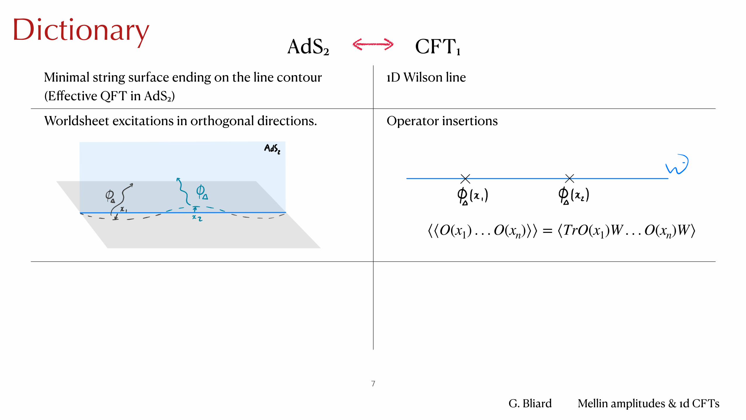
Minimal string surface ending on the line contour (Effective QFT in AdS2)
1D Wilson line
Worldsheet excitations in orthogonal directions. Operator insertions
7
AdS2 CFT1
⟨⟨O(x1) . . . O(xn)⟩⟩ = ⟨TrO(x1)W . . . O(xn)W⟩
Dictionary
G. Bliard Mellin amplitudes & 1d CFTs
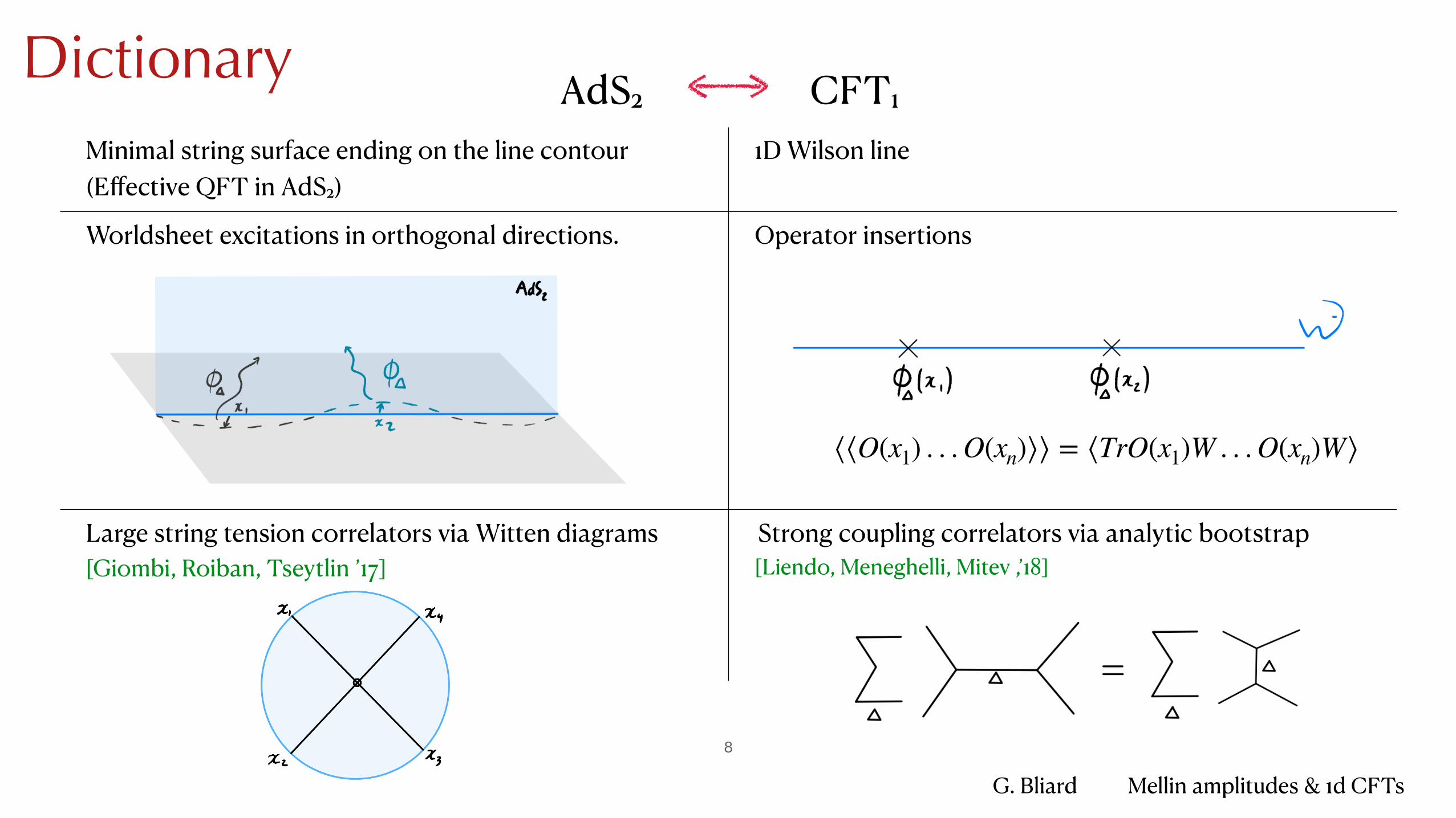
Minimal string surface ending on the line contour (Effective QFT in AdS2)
1D Wilson line
Worldsheet excitations in orthogonal directions. Operator insertions
Large string tension correlators via Witten diagrams [Giombi, Roiban, Tseytlin ’17]
Strong coupling correlators via analytic bootstrap [Liendo, Meneghelli, Mitev ,’18]
8
AdS2 CFT1
⟨⟨O(x1) . . . O(xn)⟩⟩ = ⟨TrO(x1)W . . . O(xn)W⟩
Dictionary

G. Bliard Mellin amplitudes & 1d CFTs9
OutlineMellin Transform
Why a 1d Mellin Definition and properties
Results
Example I: QFT in AdS2
Computations and Mellin CFT data
Example II: 1/2 BPS Wilson Line Witten diagrams
The Bootstrap Results and Mellin
G. Bliard Mellin amplitudes & 1d CFTs10
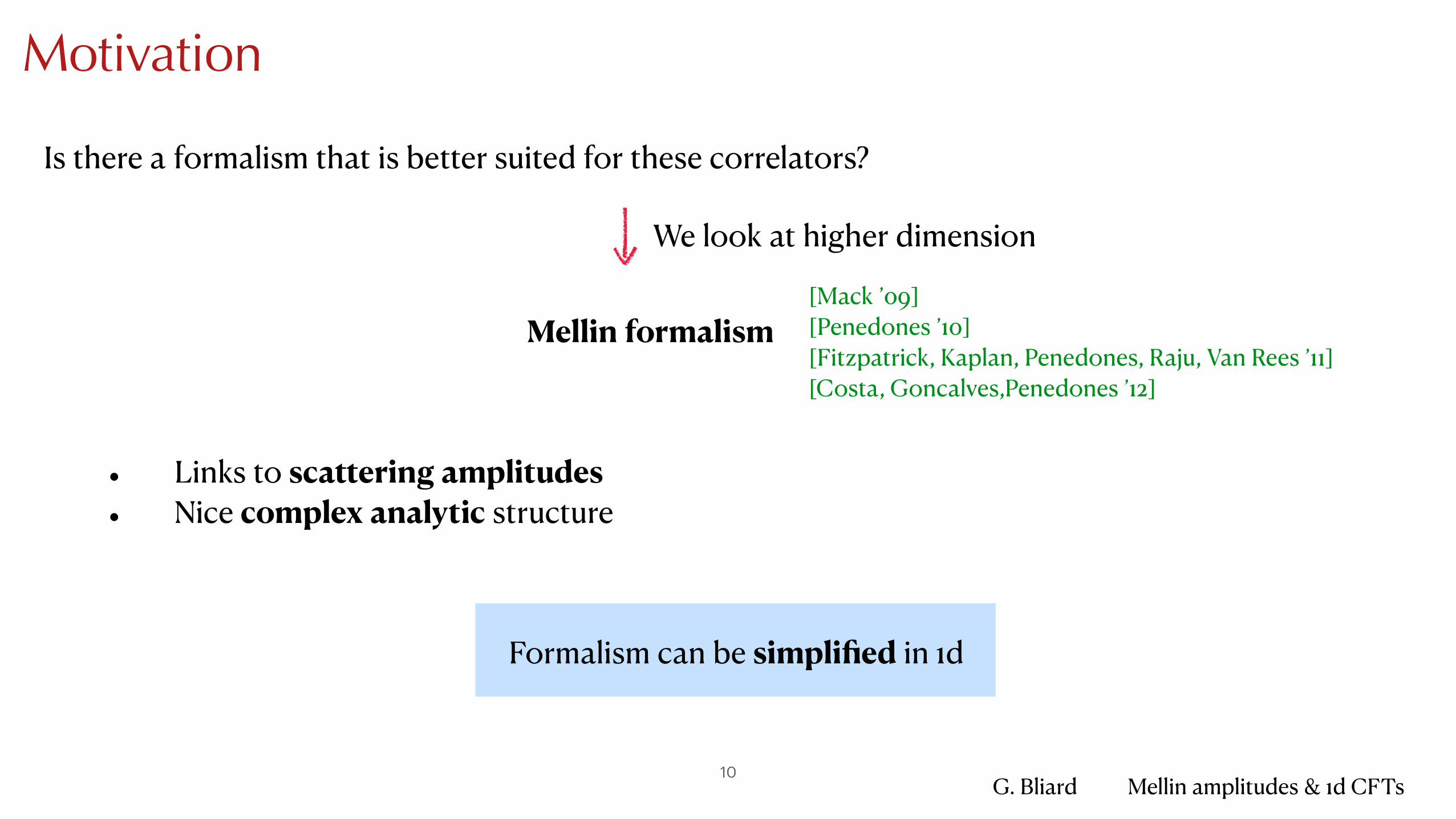
Motivation
Is there a formalism that is better suited for these correlators?
We look at higher dimension
Mellin formalism
• Links to scattering amplitudes • Nice complex analytic structure
[Mack ’09] [Penedones ’10] [Fitzpatrick, Kaplan, Penedones, Raju, Van Rees ’11] [Costa, Goncalves,Penedones ’12]
Formalism can be simplified in 1d

11
Mellin formalism in 1D
G. Bliard Mellin amplitudes & 1d CFTs12
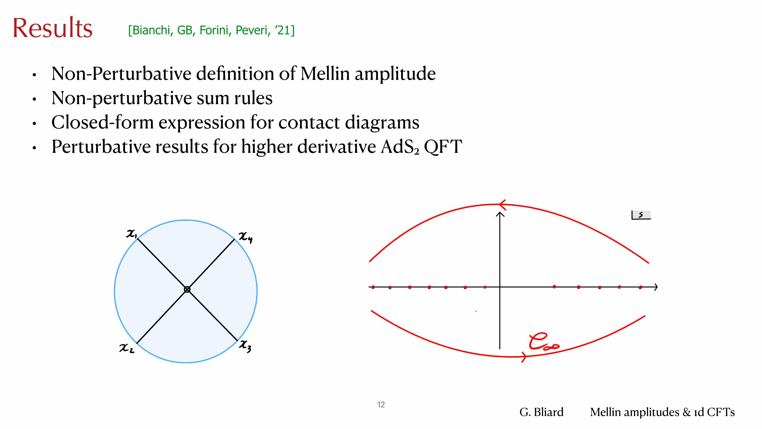
Results
• Non-Perturbative definition of Mellin amplitude • Non-perturbative sum rules • Closed-form expression for contact diagrams • Perturbative results for higher derivative AdS2 QFT
[Bianchi, GB, Forini, Peveri, ’21]
G. Bliard Mellin amplitudes & 1d CFTs13
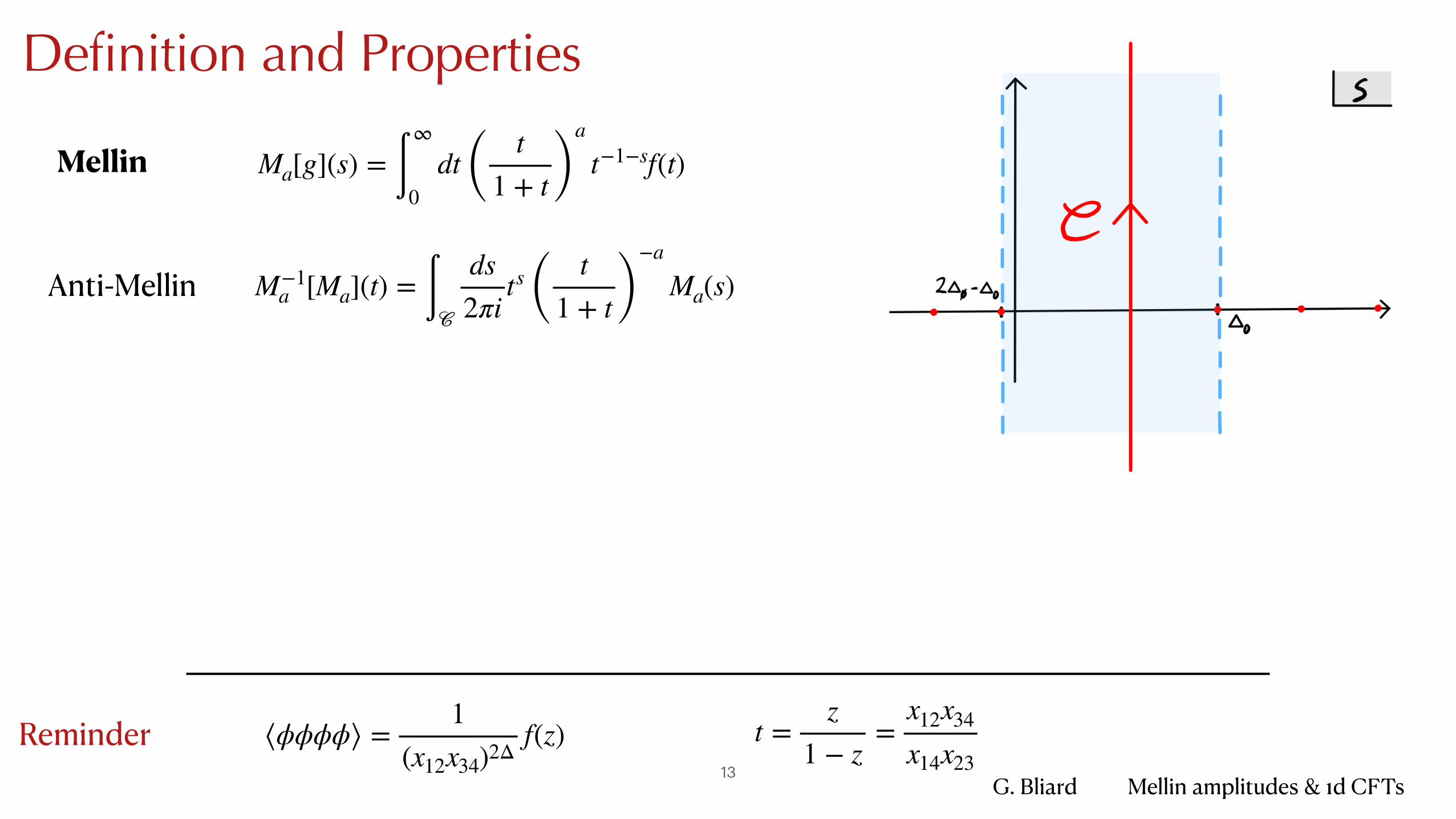
Definition and Properties
⟨ϕϕϕϕ⟩ =1
(x12x34)2Δf(z)
Ma[g](s) = ∫∞
0dt ( t
1 + t )a
t−1−sf(t)
M−1a [Ma](t) = ∫𝒞
ds2πi
ts ( t1 + t )
−a
Ma(s)
Mellin
Anti-Mellin
Reminder t =z
1 − z=
x12x34
x14x23
G. Bliard Mellin amplitudes & 1d CFTs14
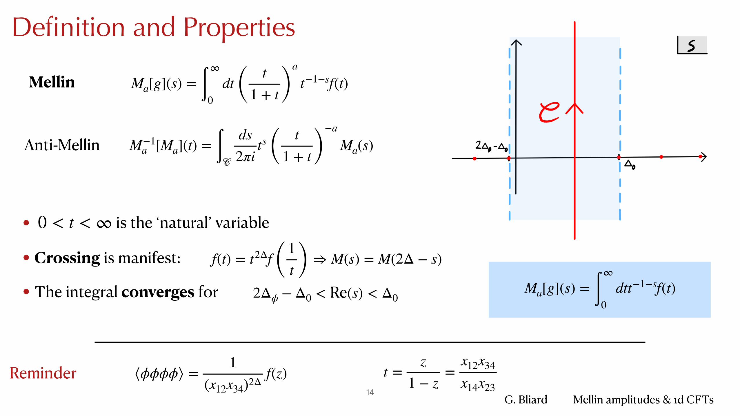
Definition and Properties
• is the ‘natural’ variable
• Crossing is manifest:
• The integral converges for
0 < t < ∞
⟨ϕϕϕϕ⟩ =1
(x12x34)2Δf(z)
Ma[g](s) = ∫∞
0dt ( t
1 + t )a
t−1−sf(t)
M−1a [Ma](t) = ∫𝒞
ds2πi
ts ( t1 + t )
−a
Ma(s)
Mellin
Anti-Mellin
Reminder
f(t) = t2Δf ( 1t ) ⇒ M(s) = M(2Δ − s)
2Δϕ − Δ0 < Re(s) < Δ0Ma[g](s) = ∫
∞
0dtt−1−sf(t)
t =z
1 − z=
x12x34
x14x23
G. Bliard Mellin amplitudes & 1d CFTs15
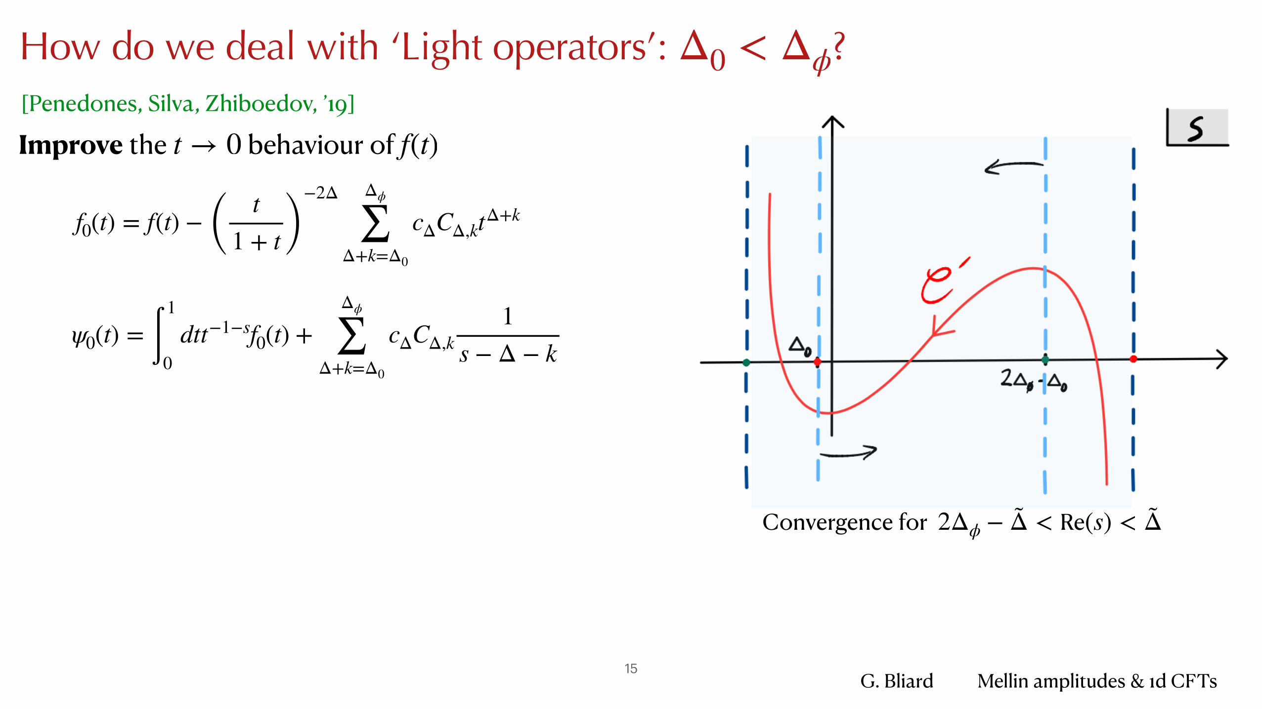
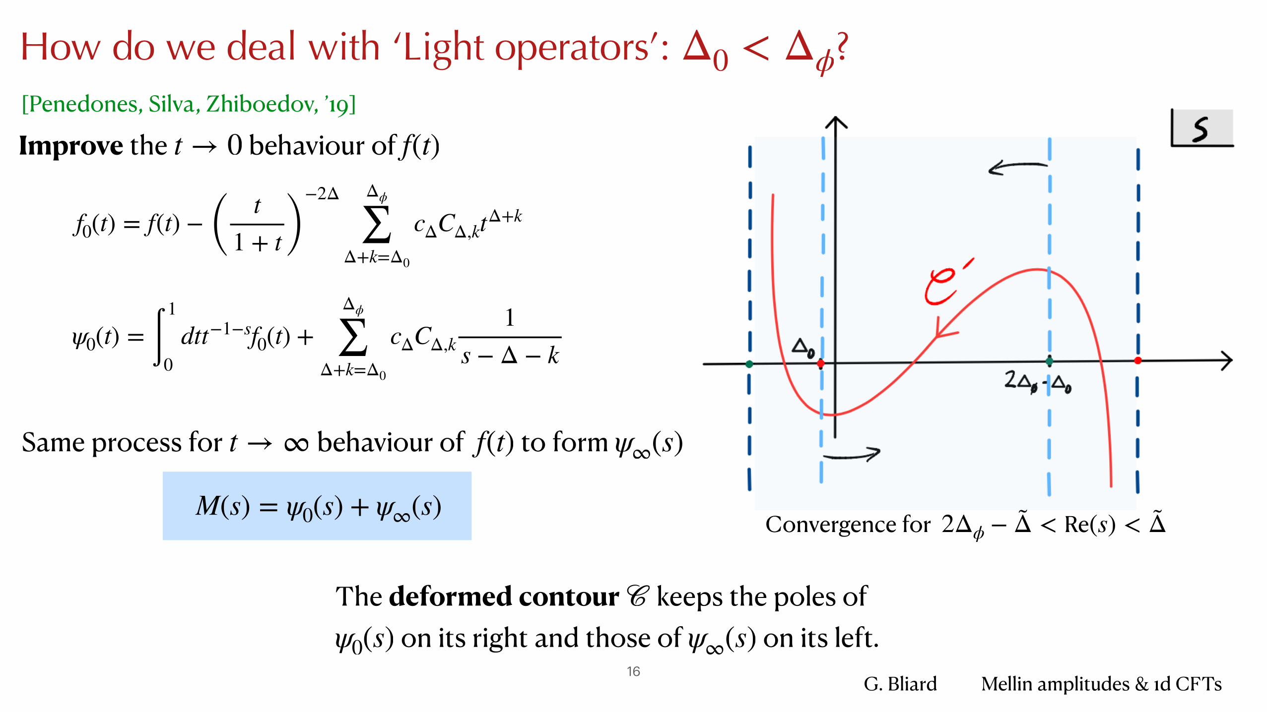
How do we deal with ‘Light operators’: ?Δ0 < Δϕ
Improve the behaviour of t → 0 f(t)
f0(t) = f(t) − ( t1 + t )
−2Δ Δϕ
∑Δ+k=Δ0
cΔCΔ,ktΔ+k
ψ0(t) = ∫1
0dtt−1−sf0(t) +
Δϕ
∑Δ+k=Δ0
cΔCΔ,k1
s − Δ − k
Convergence for 2Δϕ − Δ̃ < Re(s) < Δ̃
[Penedones, Silva, Zhiboedov, ’19]
G. Bliard Mellin amplitudes & 1d CFTs16
How do we deal with ‘Light operators’: ?Δ0 < Δϕ
Improve the behaviour of t → 0 f(t)
f0(t) = f(t) − ( t1 + t )
−2Δ Δϕ
∑Δ+k=Δ0
cΔCΔ,ktΔ+k
ψ0(t) = ∫1
0dtt−1−sf0(t) +
Δϕ
∑Δ+k=Δ0
cΔCΔ,k1
s − Δ − k
M(s) = ψ0(s) + ψ∞(s)Convergence for 2Δϕ − Δ̃ < Re(s) < Δ̃
Same process for behaviour of to form t → ∞ f(t) ψ∞(s)
The deformed contour keeps the poles of on its right and those of on its left.
𝒞ψ0(s) ψ∞(s)
[Penedones, Silva, Zhiboedov, ’19]
G. Bliard Mellin amplitudes & 1d CFTs17
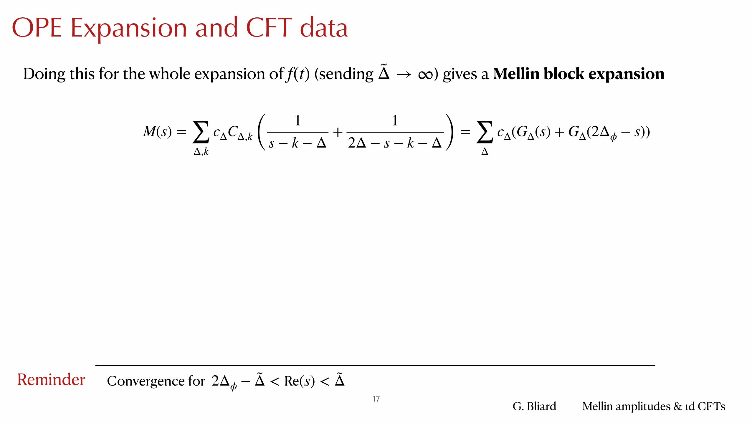
OPE Expansion and CFT data
Doing this for the whole expansion of (sending ) gives a Mellin block expansionf(t) Δ̃ → ∞
M(s) = ∑Δ,k
cΔCΔ,k ( 1s − k − Δ
+1
2Δ − s − k − Δ ) = ∑Δ
cΔ(GΔ(s) + GΔ(2Δϕ − s))
Convergence for 2Δϕ − Δ̃ < Re(s) < Δ̃Reminder
G. Bliard Mellin amplitudes & 1d CFTs18
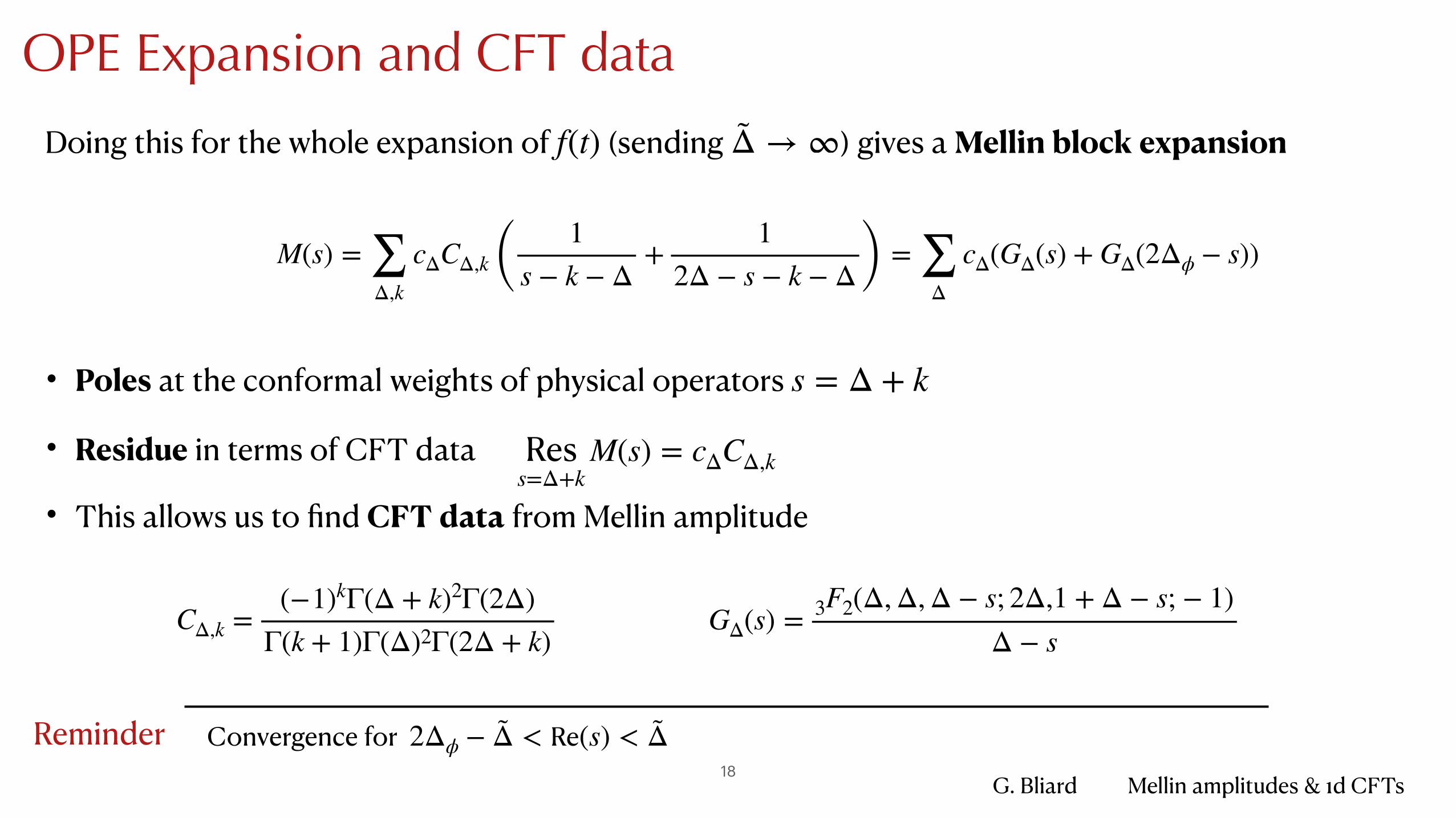
OPE Expansion and CFT data
Doing this for the whole expansion of (sending ) gives a Mellin block expansionf(t) Δ̃ → ∞
M(s) = ∑Δ,k
cΔCΔ,k ( 1s − k − Δ
+1
2Δ − s − k − Δ ) = ∑Δ
cΔ(GΔ(s) + GΔ(2Δϕ − s))
• Poles at the conformal weights of physical operators
• Residue in terms of CFT data
• This allows us to find CFT data from Mellin amplitude
s = Δ + k
Convergence for 2Δϕ − Δ̃ < Re(s) < Δ̃Reminder
CΔ,k =(−1)kΓ(Δ + k)2Γ(2Δ)
Γ(k + 1)Γ(Δ)2Γ(2Δ + k)GΔ(s) = 3F2(Δ, Δ, Δ − s; 2Δ,1 + Δ − s; − 1)
Δ − s
Ress=Δ+k
M(s) = cΔCΔ,k
G. Bliard Mellin amplitudes & 1d CFTs19
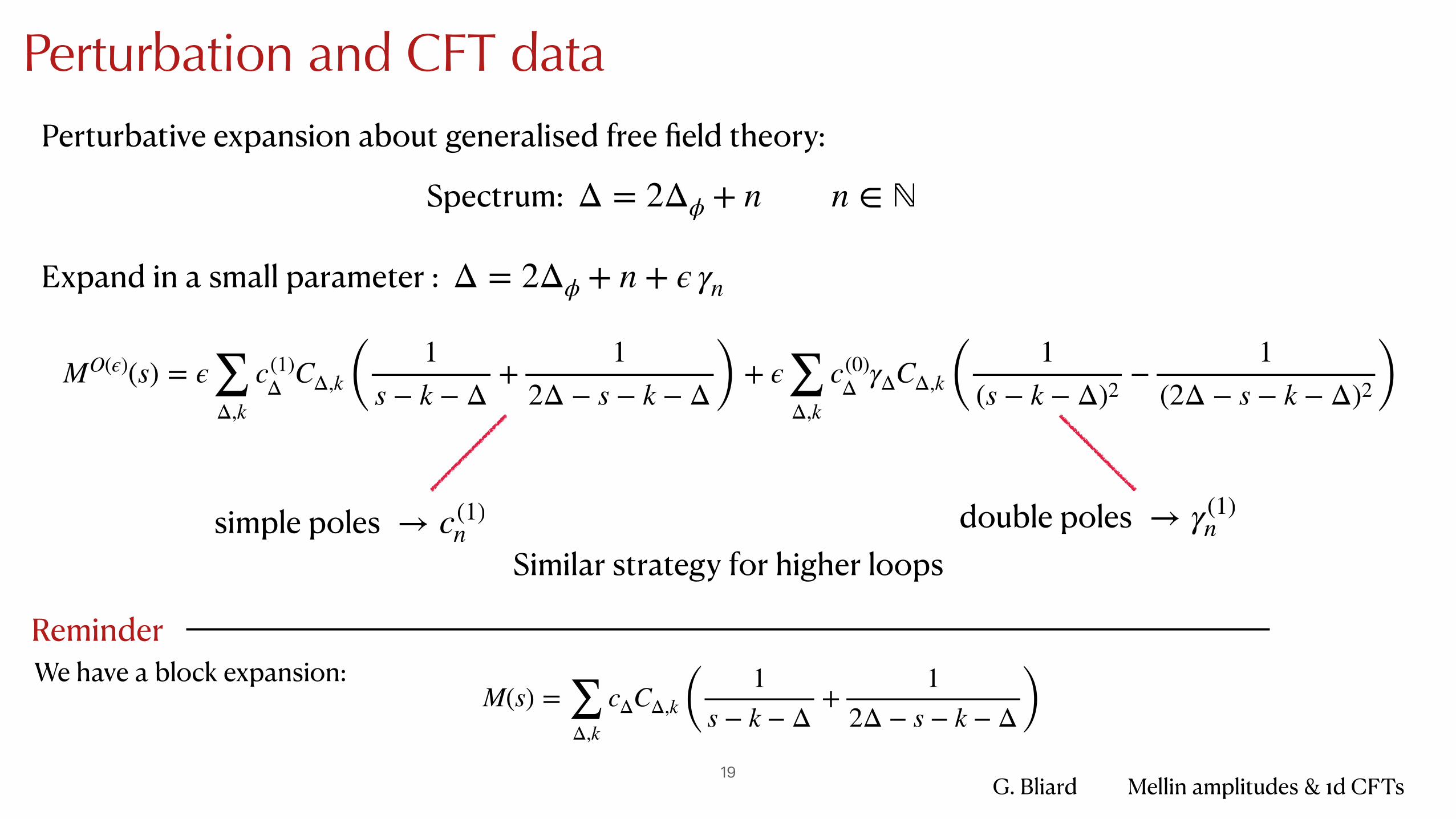
Perturbation and CFT data
Reminder
Perturbative expansion about generalised free field theory:
We have a block expansion:M(s) = ∑
Δ,k
cΔCΔ,k ( 1s − k − Δ
+1
2Δ − s − k − Δ )
Spectrum: Δ = 2Δϕ + n n ∈ ℕ
Expand in a small parameter : Δ = 2Δϕ + n + ϵ γn
MO(ϵ)(s) = ϵ∑Δ,k
c(1)Δ CΔ,k ( 1
s − k − Δ+
12Δ − s − k − Δ ) + ϵ∑
Δ,k
c(0)Δ γΔCΔ,k ( 1
(s − k − Δ)2−
1(2Δ − s − k − Δ)2 )
Similar strategy for higher loopsdouble poles → γ(1)
nsimple poles → c(1)n
G. Bliard Mellin amplitudes & 1d CFTs20
CFT1
Non-SUSY Wilson line
1/2 BPS Wilson line in 4d N=4
1/2 BPS Wilson line in 4d N=2
1/2 BPS Wilson line in ABJM
SYK models
QFT in AdS2

21
Example I: higher derivatives in AdS2
G. Bliard Mellin amplitudes & 1d CFTs22
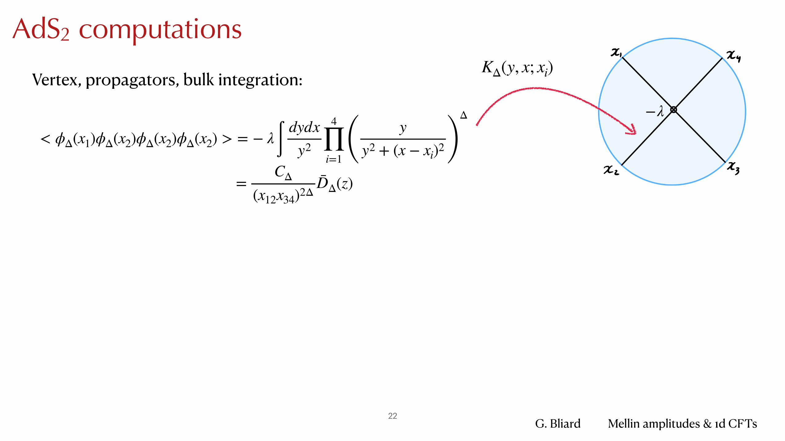
AdS2 computationsKΔ(y, x; xi)
< ϕΔ(x1)ϕΔ(x2)ϕΔ(x2)ϕΔ(x2) > = − λ∫dydx
y2
4
∏i=1 ( y
y2 + (x − xi)2 )Δ
=CΔ
(x12x34)2ΔD̄Δ(z)
−λ
Vertex, propagators, bulk integration:
G. Bliard Mellin amplitudes & 1d CFTs23
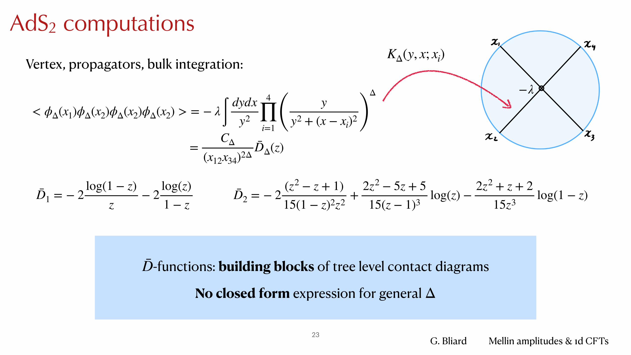
AdS2 computations
-functions: building blocks of tree level contact diagrams
No closed form expression for general
D̄
Δ
KΔ(y, x; xi)
< ϕΔ(x1)ϕΔ(x2)ϕΔ(x2)ϕΔ(x2) > = − λ∫dydx
y2
4
∏i=1 ( y
y2 + (x − xi)2 )Δ
=CΔ
(x12x34)2ΔD̄Δ(z)
−λ
Vertex, propagators, bulk integration:
D̄1 = − 2log(1 − z)
z− 2
log(z)1 − z
D̄2 = − 2(z2 − z + 1)15(1 − z)2z2
+2z2 − 5z + 515(z − 1)3
log(z) −2z2 + z + 2
15z3log(1 − z)
G. Bliard Mellin amplitudes & 1d CFTs24
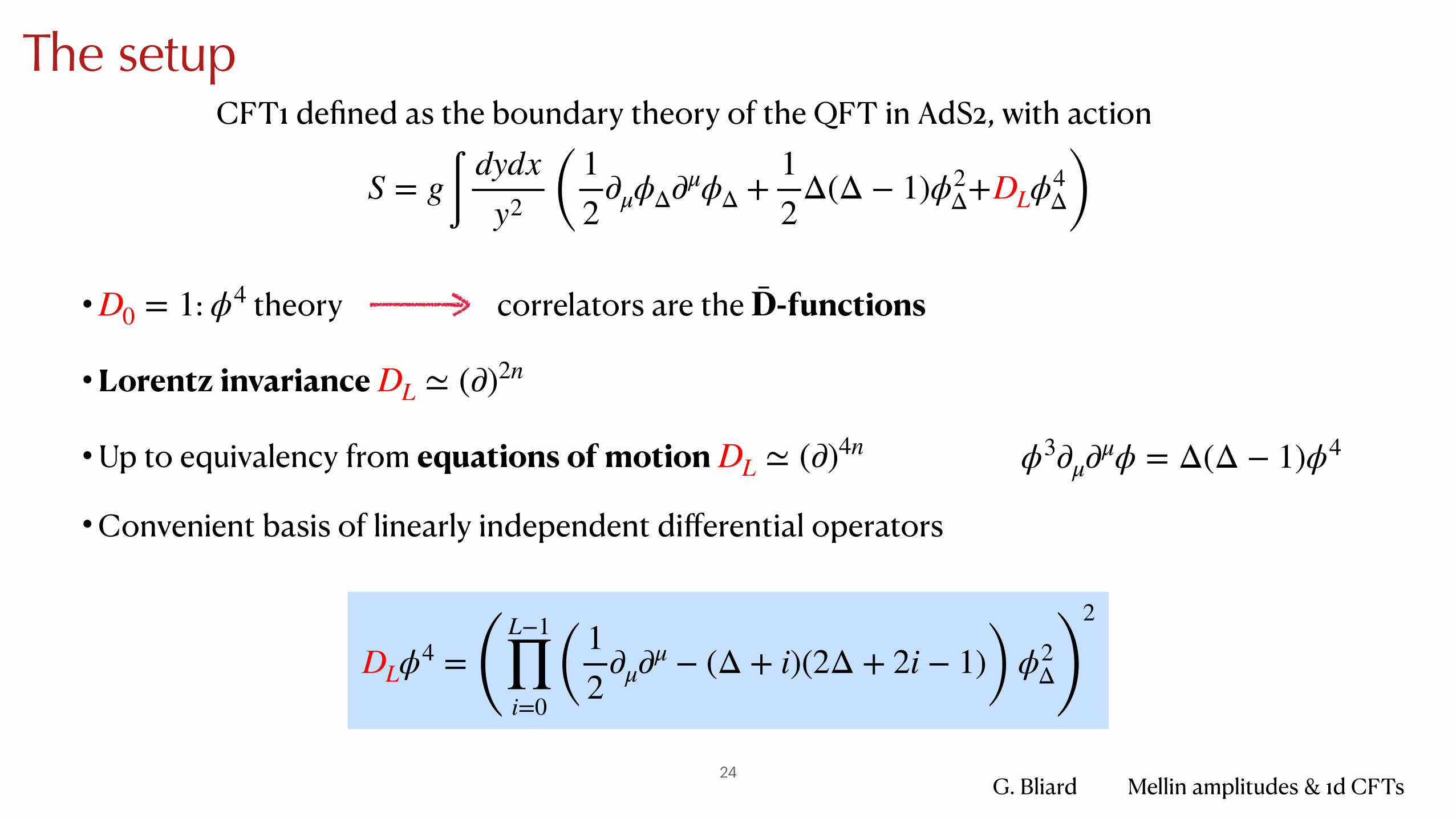
The setupCFT1 defined as the boundary theory of the QFT in AdS2, with action
S = g∫dydx
y2 ( 12
∂μϕΔ∂μϕΔ +12
Δ(Δ − 1)ϕ2Δ+DLϕ4
Δ)• : theory correlators are the -functions
•Lorentz invariance
•Up to equivalency from equations of motion
•Convenient basis of linearly independent differential operators
D0 = 1 ϕ4 D̄
DL ≃ (∂)2n
DL ≃ (∂)4n
DLϕ4 = (L−1
∏i=0
( 12
∂μ∂μ − (Δ + i)(2Δ + 2i − 1)) ϕ2Δ)
2
ϕ3∂μ∂μϕ = Δ(Δ − 1)ϕ4
G. Bliard Mellin amplitudes & 1d CFTs25
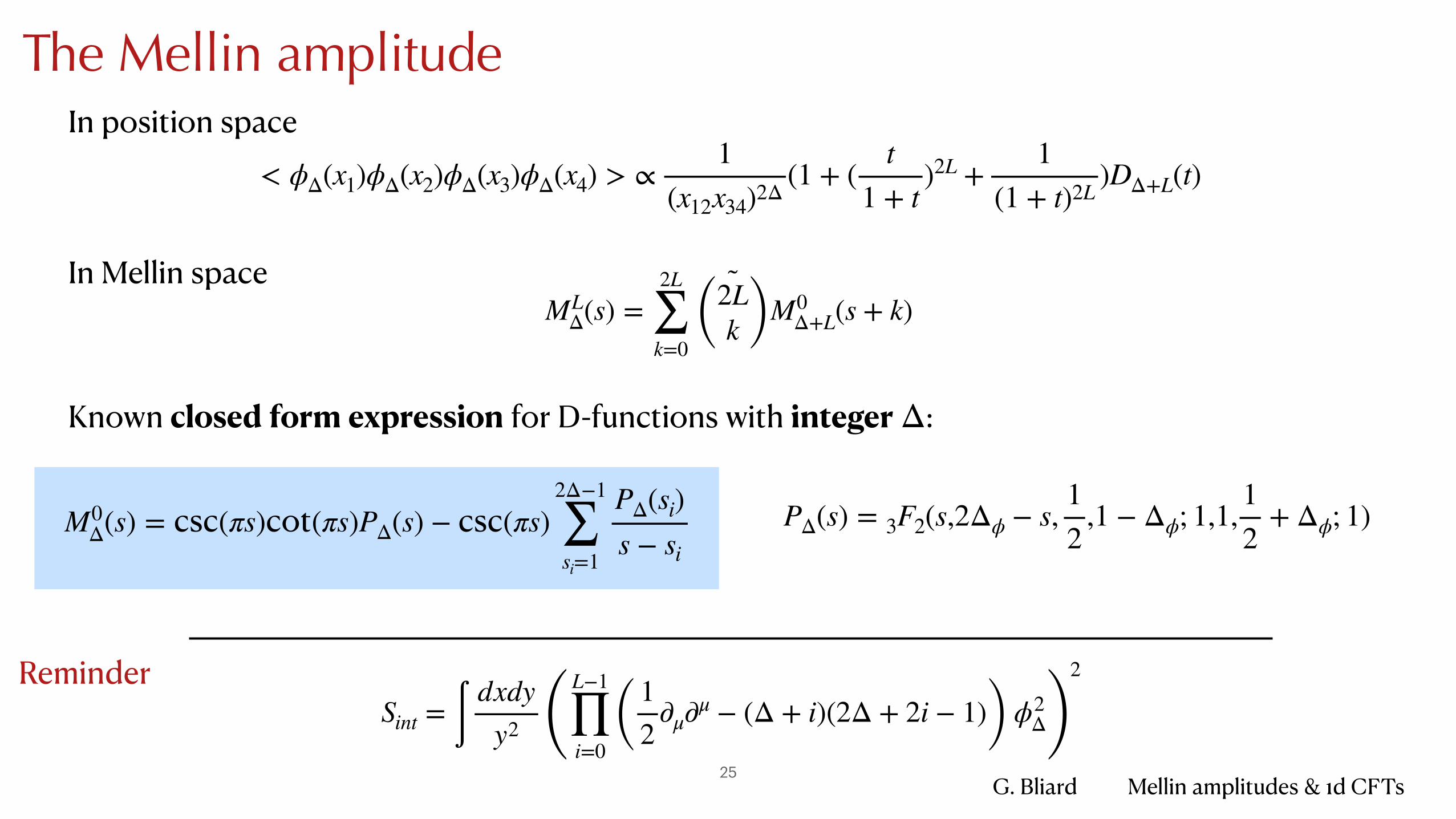
The Mellin amplitude
M0Δ(s) = csc(πs)cot(πs)PΔ(s) − csc(πs)
2Δ−1
∑si=1
PΔ(si)s − si
Known closed form expression for D-functions with integer :Δ
MLΔ(s) =
2L
∑k=0
˜(2L
k )M0Δ+L(s + k)
In position space< ϕΔ(x1)ϕΔ(x2)ϕΔ(x3)ϕΔ(x4) > ∝
1(x12x34)2Δ
(1 + (t
1 + t)2L +
1(1 + t)2L
)DΔ+L(t)
PΔ(s) = 3F2(s,2Δϕ − s,12
,1 − Δϕ; 1,1,12
+ Δϕ; 1)
ReminderSint = ∫
dxdyy2 (
L−1
∏i=0
( 12
∂μ∂μ − (Δ + i)(2Δ + 2i − 1)) ϕ2Δ)
2
In Mellin space
G. Bliard Mellin amplitudes & 1d CFTs26
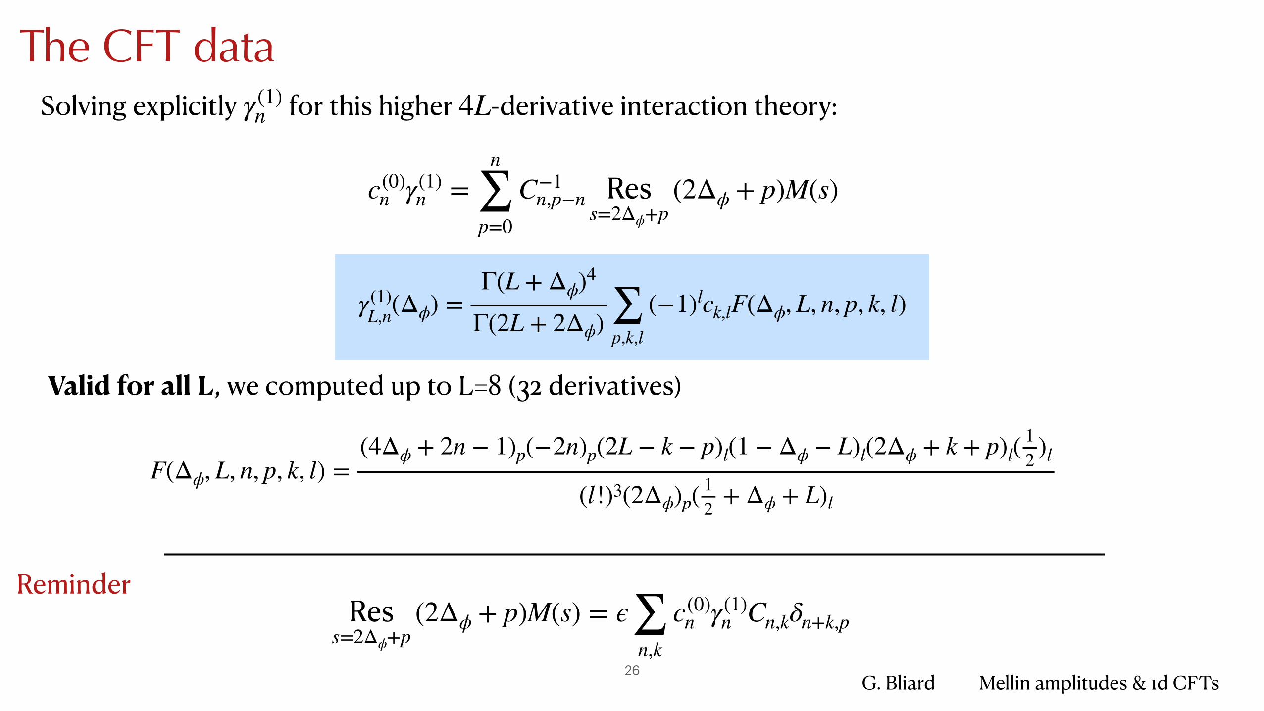
The CFT dataSolving explicitly for this higher -derivative interaction theory:γ(1)
n 4L
Reminder
c(0)n γ(1)
n =n
∑p=0
C−1n,p−n Res
s=2Δϕ+p(2Δϕ + p)M(s)
Valid for all L, we computed up to L=8 (32 derivatives)
Ress=2Δϕ+p
(2Δϕ + p)M(s) = ϵ∑n,k
c(0)n γ(1)
n Cn,kδn+k,p
γ(1)L,n(Δϕ) =
Γ(L + Δϕ)4
Γ(2L + 2Δϕ) ∑p,k,l
(−1)lck,lF(Δϕ, L, n, p, k, l)
F(Δϕ, L, n, p, k, l) =(4Δϕ + 2n − 1)p(−2n)p(2L − k − p)l(1 − Δϕ − L)l(2Δϕ + k + p)l(
12 )l
(l!)3(2Δϕ)p( 12 + Δϕ + L)l
G. Bliard Mellin amplitudes & 1d CFTs27
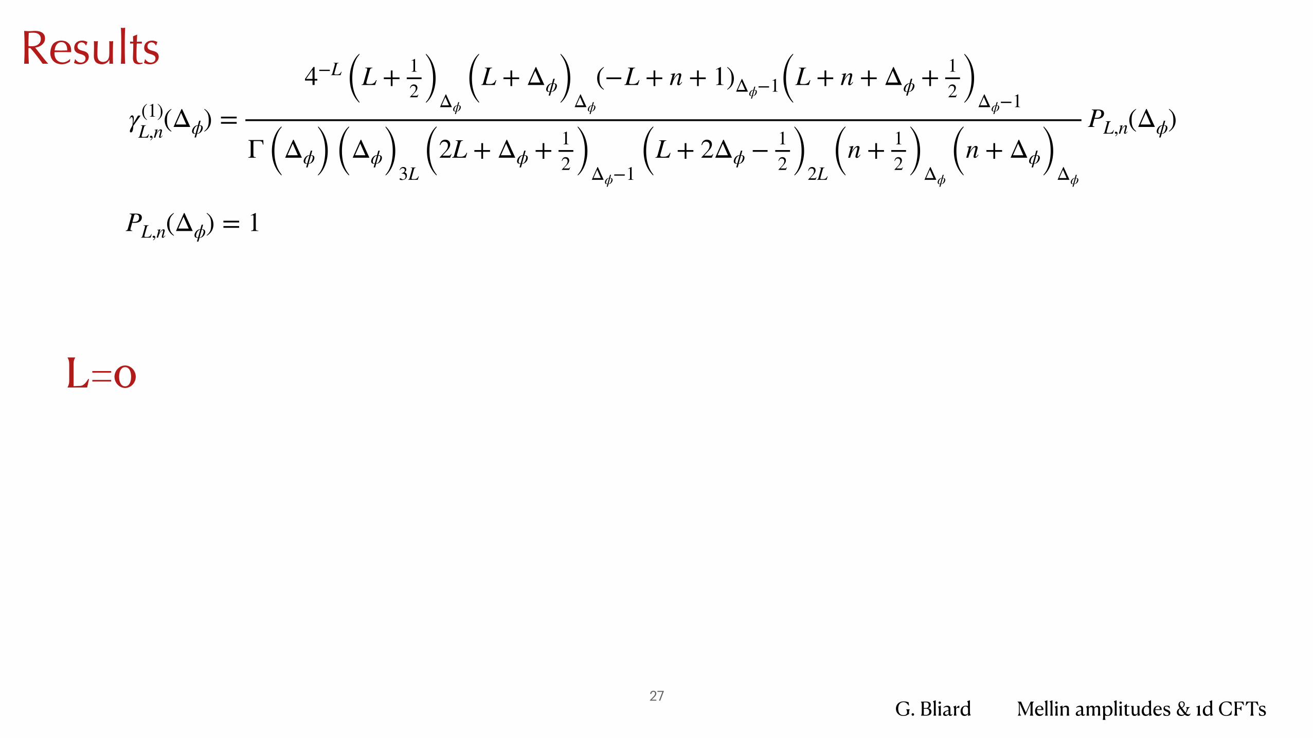
Resultsγ(1)L,n(Δϕ) =
4−L (L + 12 )Δϕ
(L + Δϕ)Δϕ
(−L + n + 1)Δϕ−1(L + n + Δϕ + 12 )Δϕ−1
Γ (Δϕ) (Δϕ)3L (2L + Δϕ + 12 )Δϕ−1 (L + 2Δϕ − 1
2 )2L (n + 12 )Δϕ
(n + Δϕ)Δϕ
PL,n(Δϕ)
PL,n(Δϕ) = 1
L=0
G. Bliard Mellin amplitudes & 1d CFTs28
Resultsγ(1)L,n(Δϕ) =
4−L (L + 12 )Δϕ
(L + Δϕ)Δϕ
(−L + n + 1)Δϕ−1(L + n + Δϕ + 12 )Δϕ−1
Γ (Δϕ) (Δϕ)3L (2L + Δϕ + 12 )Δϕ−1 (L + 2Δϕ − 1
2 )2L (n + 12 )Δϕ
(n + Δϕ)Δϕ
𝒫L,n(Δϕ)
PL,n(Δϕ)
L=1
G. Bliard Mellin amplitudes & 1d CFTs29
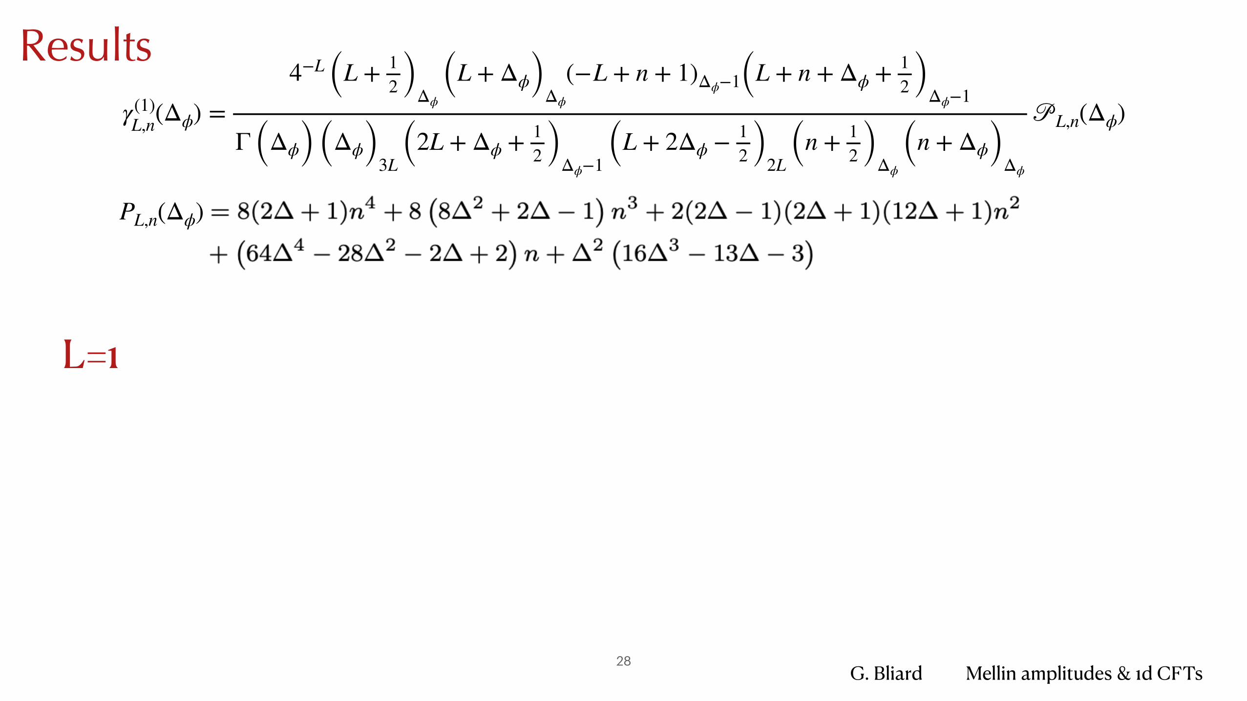
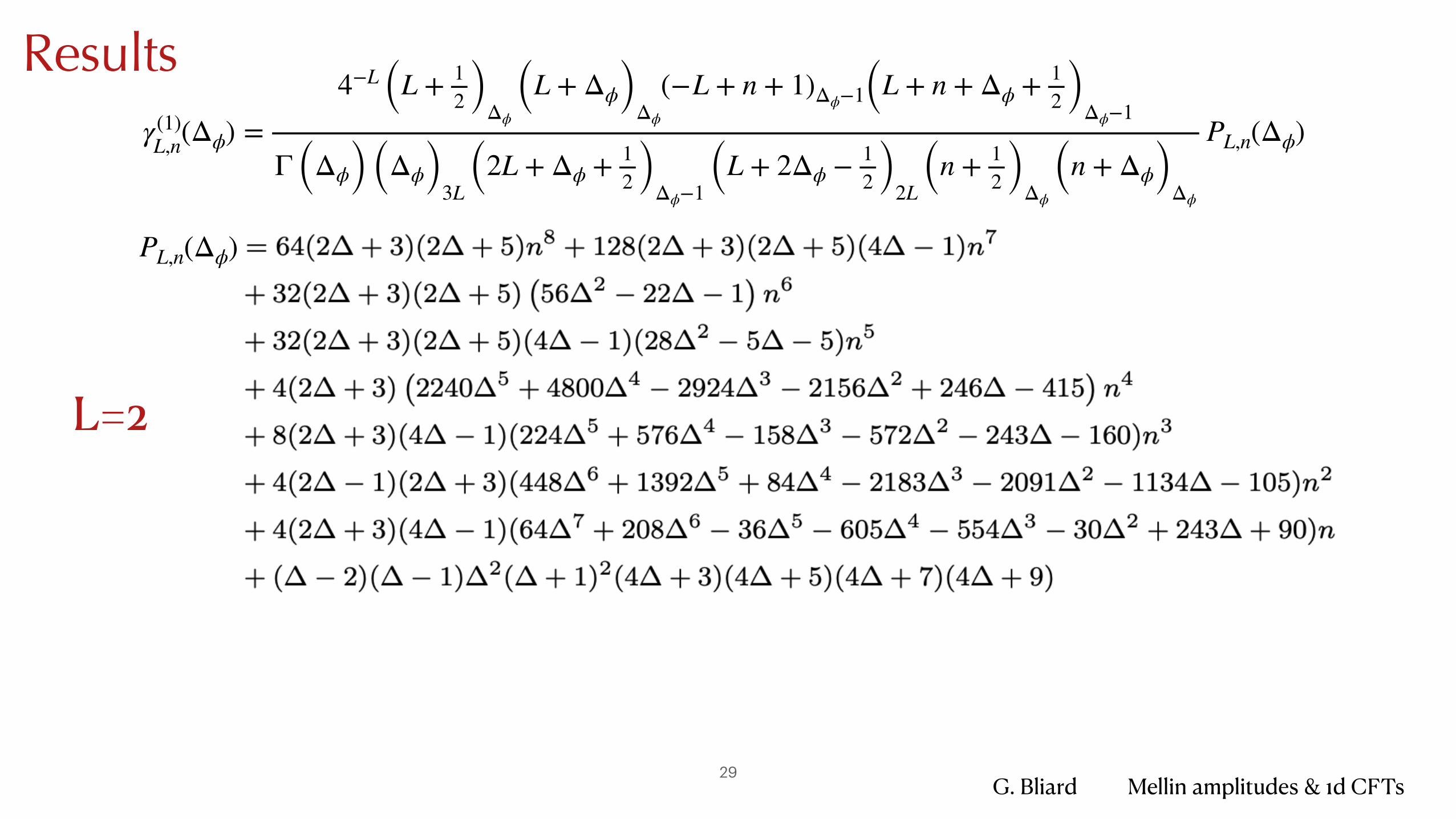
Resultsγ(1)L,n(Δϕ) =
4−L (L + 12 )Δϕ
(L + Δϕ)Δϕ
(−L + n + 1)Δϕ−1(L + n + Δϕ + 12 )Δϕ−1
Γ (Δϕ) (Δϕ)3L (2L + Δϕ + 12 )Δϕ−1 (L + 2Δϕ − 1
2 )2L (n + 12 )Δϕ
(n + Δϕ)Δϕ
PL,n(Δϕ)
PL,n(Δϕ)
L=2
G. Bliard Mellin amplitudes & 1d CFTs30
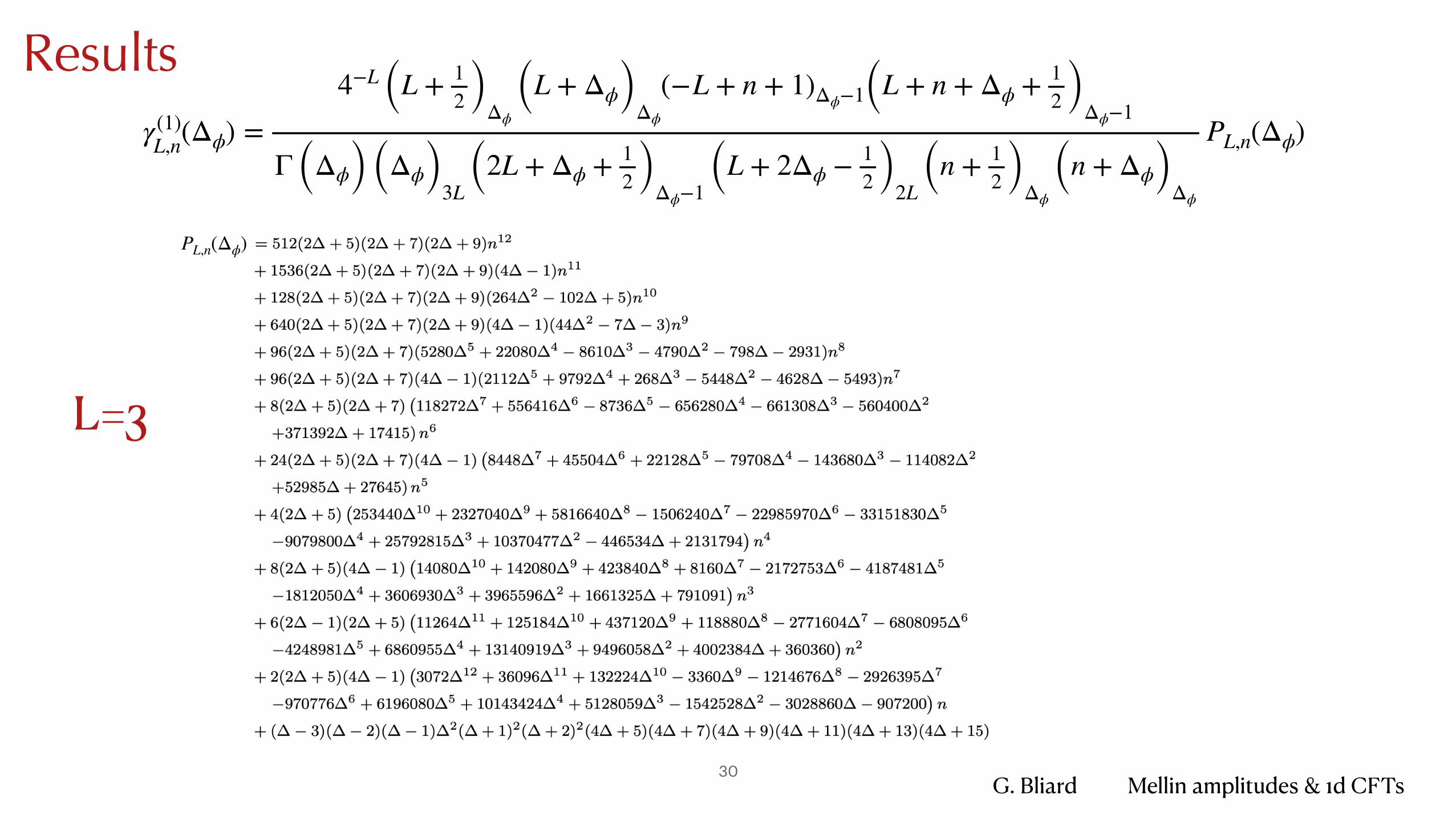
Resultsγ(1)L,n(Δϕ) =
4−L (L + 12 )Δϕ
(L + Δϕ)Δϕ
(−L + n + 1)Δϕ−1(L + n + Δϕ + 12 )Δϕ−1
Γ (Δϕ) (Δϕ)3L (2L + Δϕ + 12 )Δϕ−1 (L + 2Δϕ − 1
2 )2L (n + 12 )Δϕ
(n + Δϕ)Δϕ
PL,n(Δϕ)
P0,n(Δϕ) = 1
PL,n(Δϕ)
L=3
G. Bliard Mellin amplitudes & 1d CFTs31
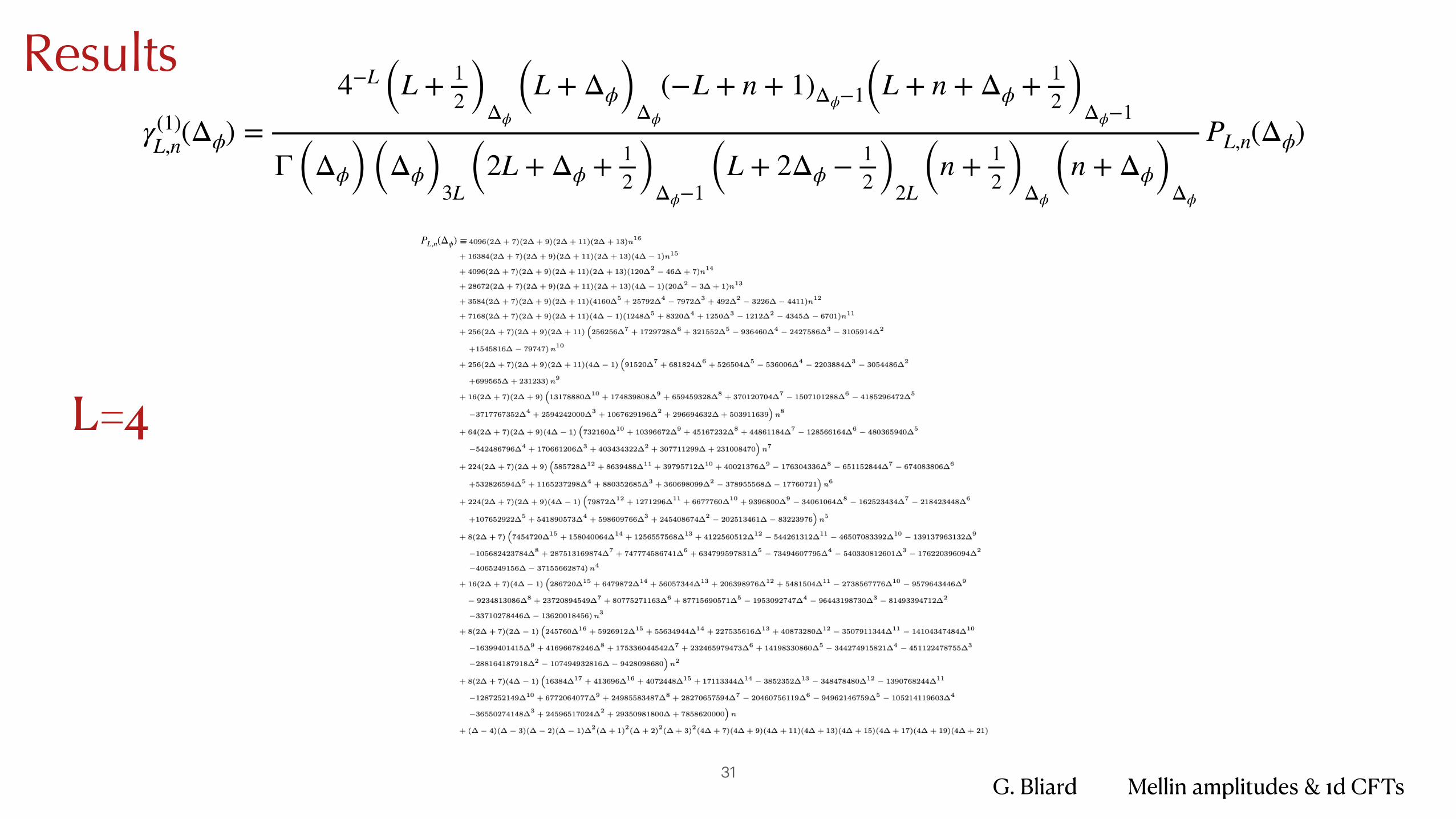
Resultsγ(1)L,n(Δϕ) =
4−L (L + 12 )Δϕ
(L + Δϕ)Δϕ
(−L + n + 1)Δϕ−1(L + n + Δϕ + 12 )Δϕ−1
Γ (Δϕ) (Δϕ)3L (2L + Δϕ + 12 )Δϕ−1 (L + 2Δϕ − 1
2 )2L (n + 12 )Δϕ
(n + Δϕ)Δϕ
PL,n(Δϕ)
PL,n(Δϕ) =
L=4
32
Example II: ABJM 1/2 BPS Wilson line
G. Bliard Mellin amplitudes & 1d CFTs
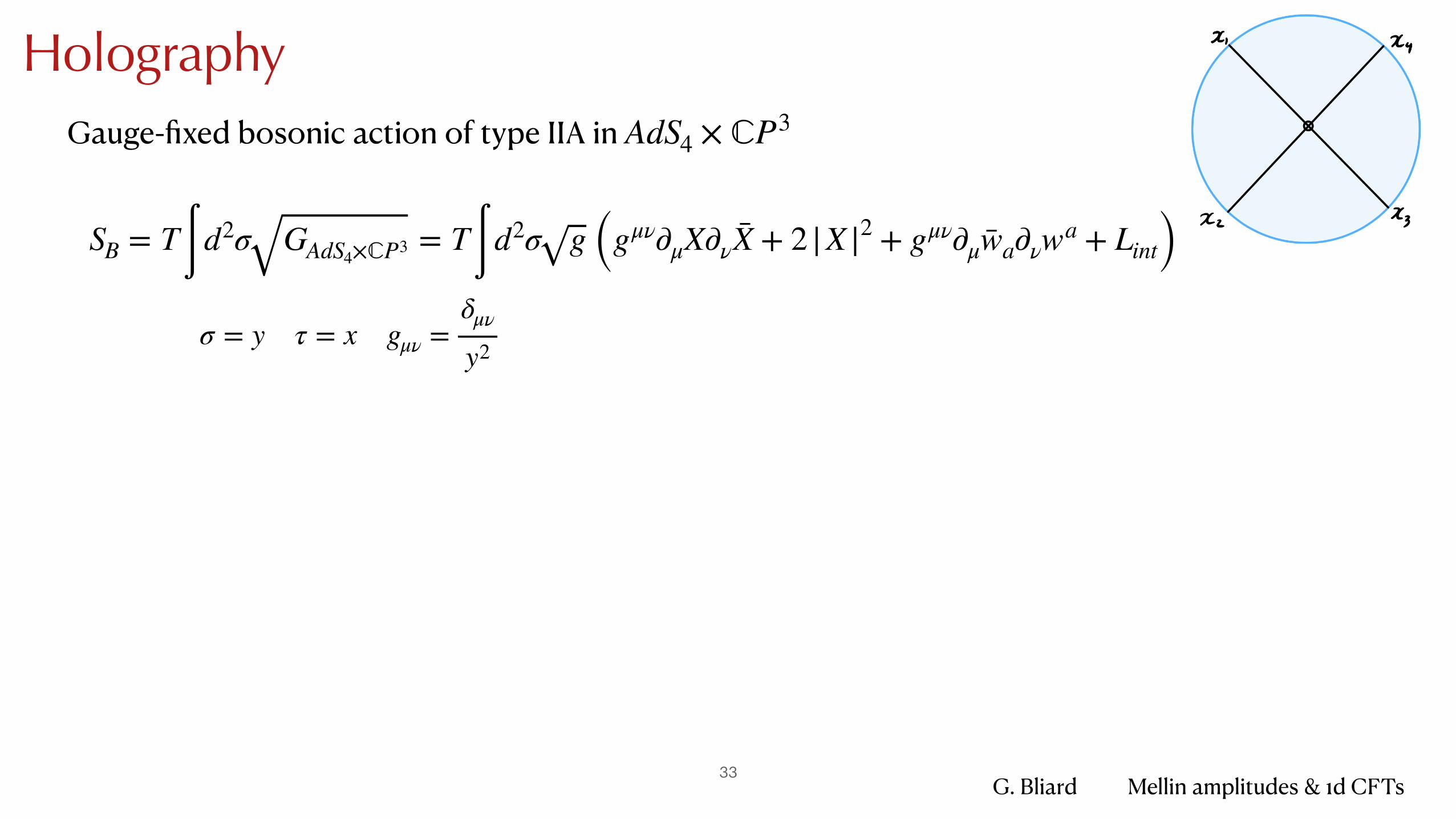
Gauge-fixed bosonic action of type IIA in AdS4 × ℂP3
33
Holography
σ = y τ = x gμν =δμν
y2
SB = T∫ d2σ GAdS4×ℂP3 = T∫ d2σ g (gμν∂μX∂νX̄ + 2 |X |2 + gμν∂μw̄a∂νwa + Lint)
G. Bliard Mellin amplitudes & 1d CFTs
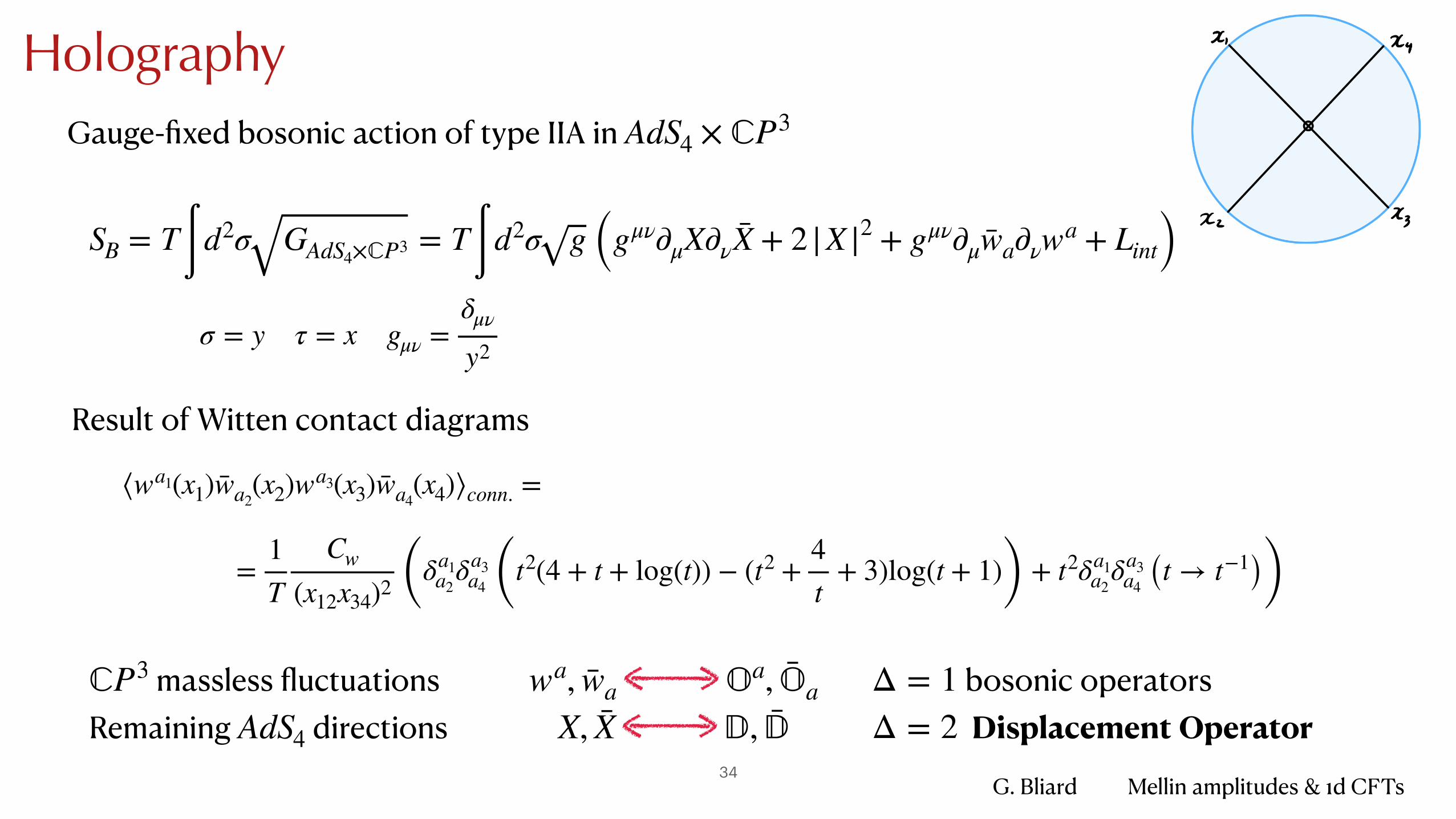
Gauge-fixed bosonic action of type IIA in AdS4 × ℂP3
34
Holography
σ = y τ = x gμν =δμν
y2
SB = T∫ d2σ GAdS4×ℂP3 = T∫ d2σ g (gμν∂μX∂νX̄ + 2 |X |2 + gμν∂μw̄a∂νwa + Lint)
Result of Witten contact diagrams
⟨wa1(x1)w̄a2(x2)wa3(x3)w̄a4
(x4)⟩conn. =
massless fluctuations Remaining directions ℂP3
AdS4
=1T
Cw
(x12x34)2 (δa1a2
δa3a4 (t2(4 + t + log(t)) − (t2 +
4t
+ 3)log(t + 1)) + t2δa1a2
δa3a4 (t → t−1))
bosonic operators Displacement Operator
Δ = 1Δ = 2
wa, w̄a 𝕆a, �̄�aX, X̄ 𝔻, �̄�
G. Bliard Mellin amplitudes & 1d CFTs35
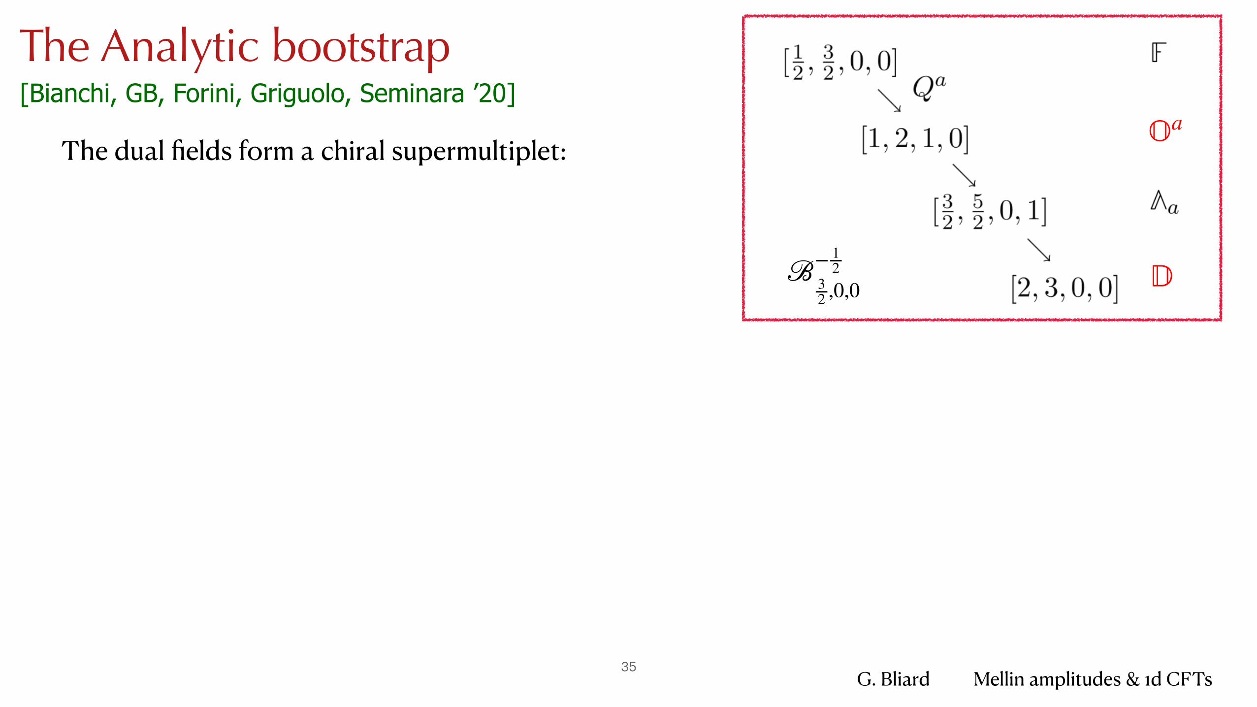
The Analytic bootstrap
The dual fields form a chiral supermultiplet:
ℬ− 12
32 ,0,0
𝕆a
𝔻
[Bianchi, GB, Forini, Griguolo, Seminara ’20]
G. Bliard Mellin amplitudes & 1d CFTs36
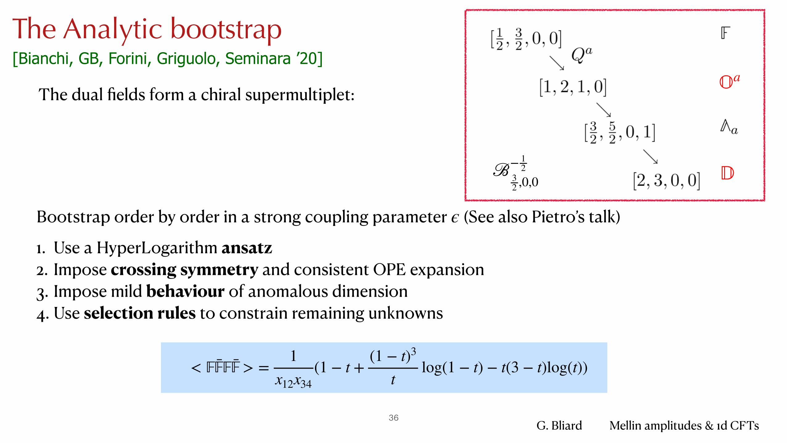
The Analytic bootstrap
The dual fields form a chiral supermultiplet:
Bootstrap order by order in a strong coupling parameter (See also Pietro’s talk)
ϵ
< 𝔽𝔽𝔽𝔽 > =1
x12x34(1 − t +
(1 − t)3
tlog(1 − t) − t(3 − t)log(t))
ℬ− 12
32 ,0,0
1. Use a HyperLogarithm ansatz 2. Impose crossing symmetry and consistent OPE expansion 3. Impose mild behaviour of anomalous dimension 4. Use selection rules to constrain remaining unknowns
𝕆a
𝔻
[Bianchi, GB, Forini, Griguolo, Seminara ’20]

G. Bliard Mellin amplitudes & 1d CFTs37
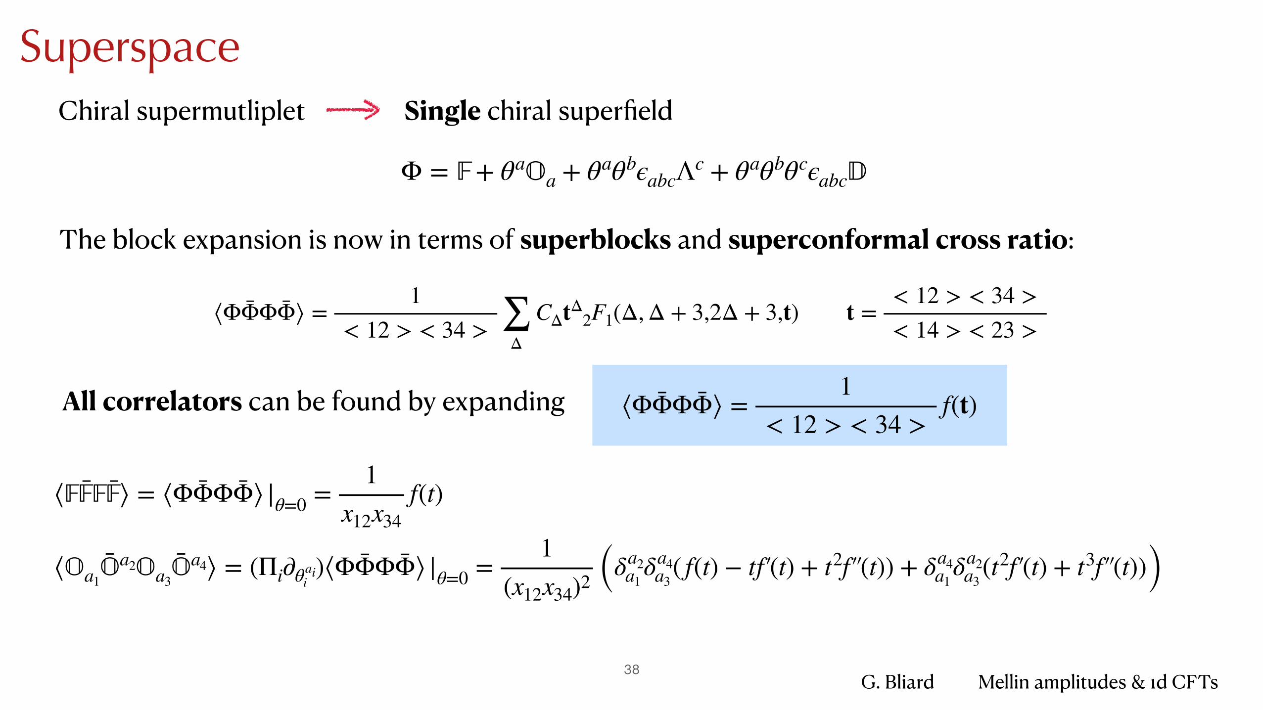
SuperspaceChiral supermutliplet Single chiral superfield
Φ = 𝔽 + θa𝕆a + θaθbϵabcΛc + θaθbθcϵabc𝔻
The block expansion is now in terms of superblocks and superconformal cross ratio:
⟨ΦΦ̄ΦΦ̄⟩ =1
< 12 > < 34 > ∑Δ
CΔtΔ2F1(Δ, Δ + 3,2Δ + 3,t) t =
< 12 > < 34 >< 14 > < 23 >
G. Bliard Mellin amplitudes & 1d CFTs38
SuperspaceChiral supermutliplet Single chiral superfield
Φ = 𝔽 + θa𝕆a + θaθbϵabcΛc + θaθbθcϵabc𝔻
The block expansion is now in terms of superblocks and superconformal cross ratio:
⟨ΦΦ̄ΦΦ̄⟩ =1
< 12 > < 34 > ∑Δ
CΔtΔ2F1(Δ, Δ + 3,2Δ + 3,t) t =
< 12 > < 34 >< 14 > < 23 >
All correlators can be found by expanding
⟨𝔽𝔽𝔽𝔽⟩ = ⟨ΦΦ̄ΦΦ̄⟩ |θ=0 =1
x12x34f(t)
⟨𝕆a1�̄�a2𝕆a3
�̄�a4⟩ = (Πi∂θaii)⟨ΦΦ̄ΦΦ̄⟩ |θ=0 =
1(x12x34)2 (δa2
a1δa4
a3( f(t) − tf′ (t) + t2f′ ′ (t)) + δa4
a1δa2
a3(t2f′ (t) + t3f′ ′ (t)))
⟨ΦΦ̄ΦΦ̄⟩ =1
< 12 > < 34 >f(t)
G. Bliard Mellin amplitudes & 1d CFTs39
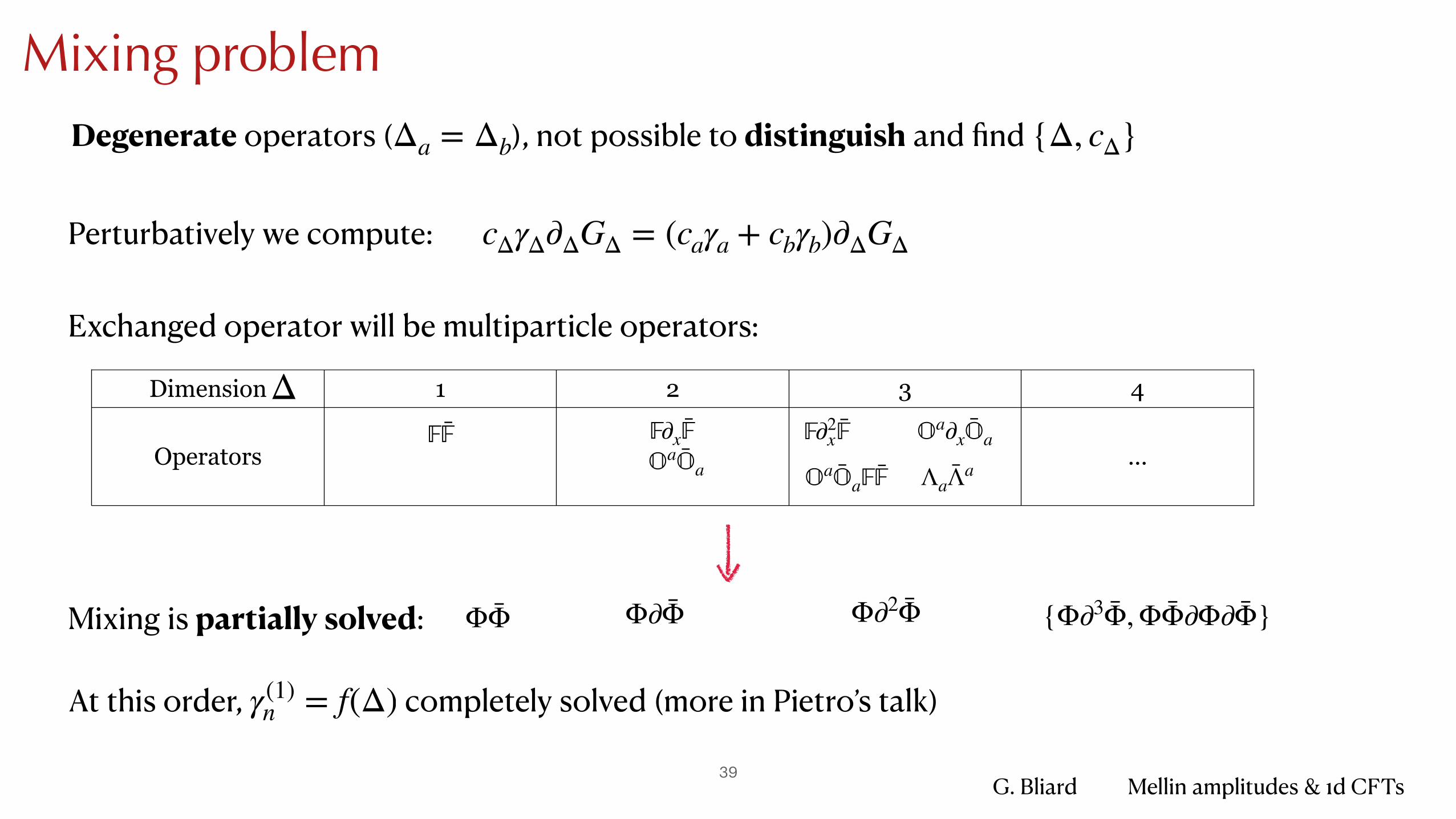
Mixing problem
Exchanged operator will be multiparticle operators:
Dimension 1 2 3 4
Operators …
Δ𝔽𝔽 𝔽∂x𝔽
𝕆a�̄�a
𝔽∂2x𝔽 𝕆a∂x�̄�a
𝕆a�̄�a𝔽𝔽 ΛaΛ̄a
Degenerate operators ( ), not possible to distinguish and find Δa = Δb {Δ, cΔ}
Perturbatively we compute: cΔγΔ∂ΔGΔ = (caγa + cbγb)∂ΔGΔ
Mixing is partially solved: {Φ∂3Φ̄, ΦΦ̄∂Φ∂Φ̄}ΦΦ̄ Φ∂Φ̄ Φ∂2Φ̄
At this order, completely solved (more in Pietro’s talk)γ(1)n = f(Δ)
G. Bliard Mellin amplitudes & 1d CFTs40
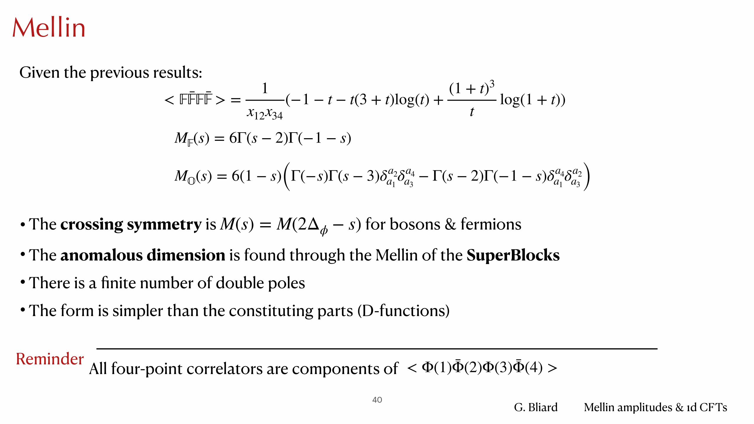
Mellin
Reminder < Φ(1)Φ̄(2)Φ(3)Φ̄(4) >All four-point correlators are components of
40
< 𝔽𝔽𝔽𝔽 > =1
x12x34(−1 − t − t(3 + t)log(t) +
(1 + t)3
tlog(1 + t))
Given the previous results:
M𝔽(s) = 6Γ(s − 2)Γ(−1 − s)
M𝕆(s) = 6(1 − s)(Γ(−s)Γ(s − 3)δa2a1
δa4a3
− Γ(s − 2)Γ(−1 − s)δa4a1
δa2a3 )
•The crossing symmetry is for bosons & fermions
•The anomalous dimension is found through the Mellin of the SuperBlocks •There is a finite number of double poles •The form is simpler than the constituting parts (D-functions)
M(s) = M(2Δϕ − s)
G. Bliard Mellin amplitudes & 1d CFTs41
Conclusions
• a Simple analytic structure • Poles at the weights of the physical operators • Consistent bloc expansion
• The ‘building blocks’ D-functions have a closed-form expression for integer
• Anomalous dimensions in higher 4L-derivative model.
• st order analysis of ABJM 1/2 BPS Wilson line insertions
• Superspace structure solves mixing and relates mellin amplitudes
Δ
1
In the context of the study of CFT1 theories, there is an array of tools to compute the CFT data (Witten diagrams, Analytric bootstrap, Mellin amplitudes). Propose a new tool, the 1d Mellin formalism for 4 point correlators with
G. Bliard Mellin amplitudes & 1d CFTs42
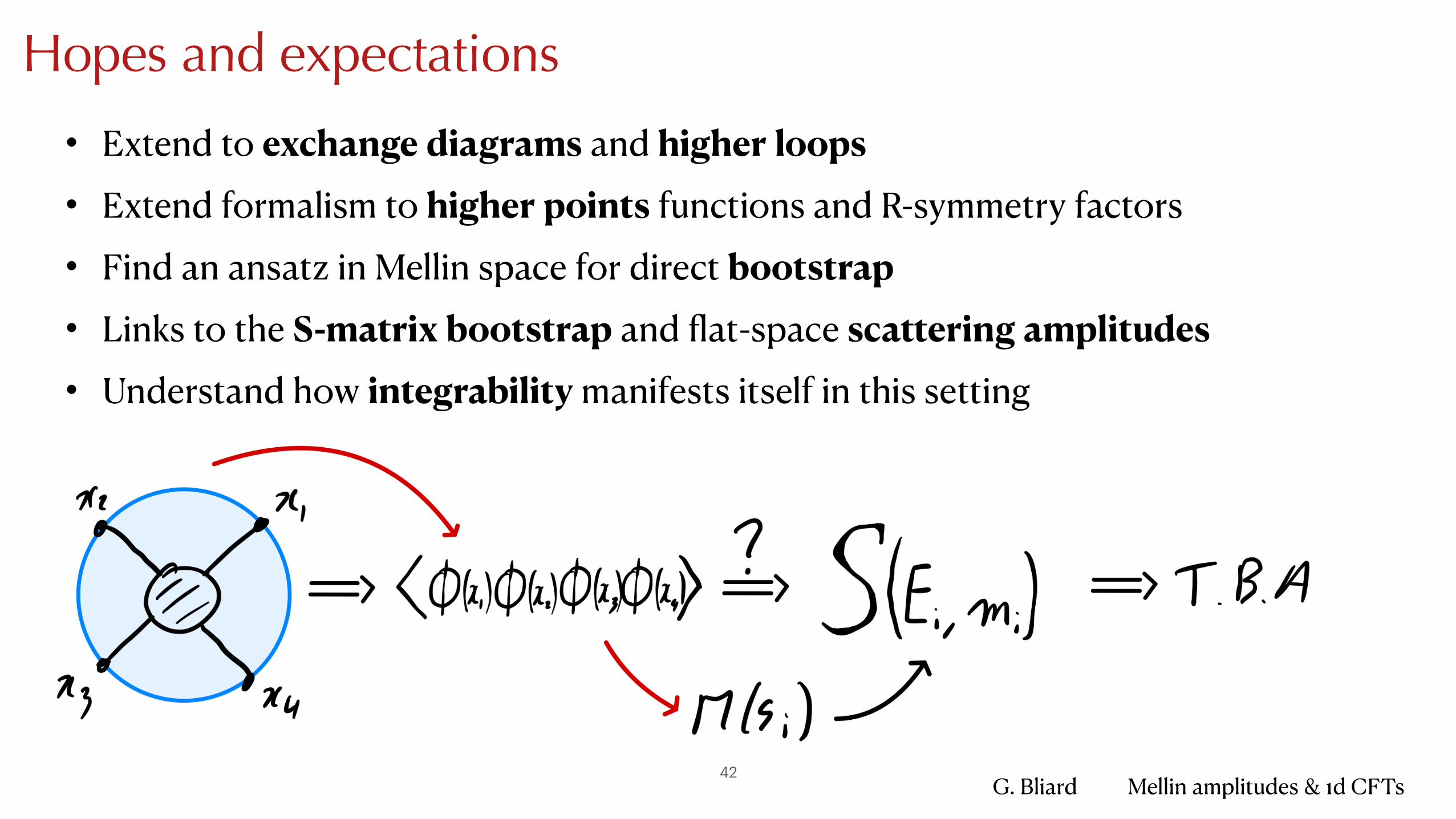
Hopes and expectations
• Extend to exchange diagrams and higher loops
• Extend formalism to higher points functions and R-symmetry factors
• Find an ansatz in Mellin space for direct bootstrap
• Links to the S-matrix bootstrap and flat-space scattering amplitudes
• Understand how integrability manifests itself in this setting

43
hank you!
G. Bliard Mellin amplitudes & 1d CFTs44
CFT1
x2P x12
I x−112
P x−112 − x−1
14I 1
x−112 − x−1
14
D x−113 − x−1
14
x−112 − x−1
14=
x12x34
x13x24= χ =
tt + 1
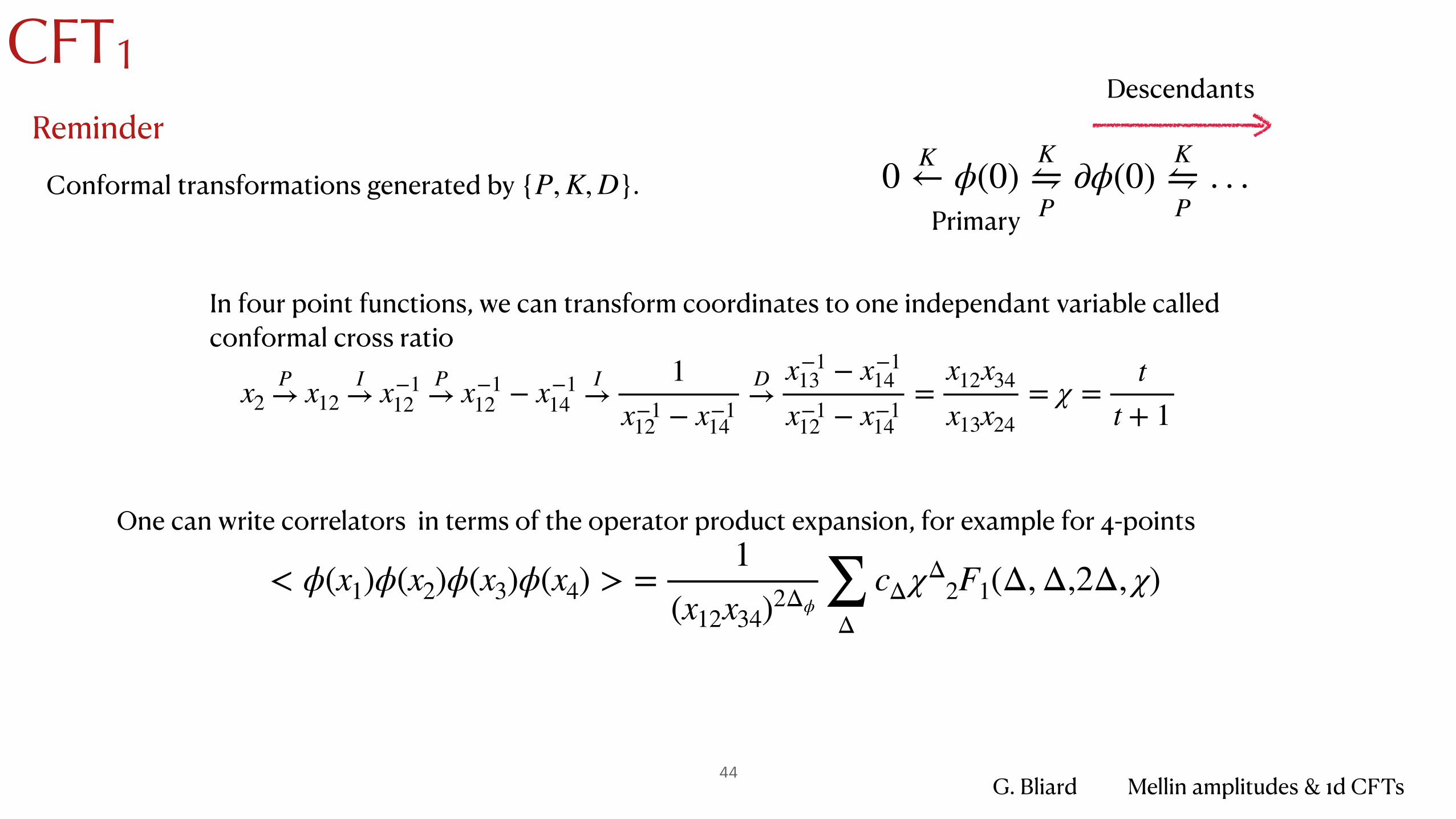
In four point functions, we can transform coordinates to one independant variable called conformal cross ratio
Conformal transformations generated by .{P, K, D} 0 K← ϕ(0)K⇋P
∂ϕ(0)K⇋P
. . .Reminder
Primary
Descendants
One can write correlators in terms of the operator product expansion, for example for 4-points
< ϕ(x1)ϕ(x2)ϕ(x3)ϕ(x4) > =1
(x12x34)2Δϕ ∑Δ
cΔχΔ2F1(Δ, Δ,2Δ, χ)
G. Bliard Mellin amplitudes & 1d CFTs45
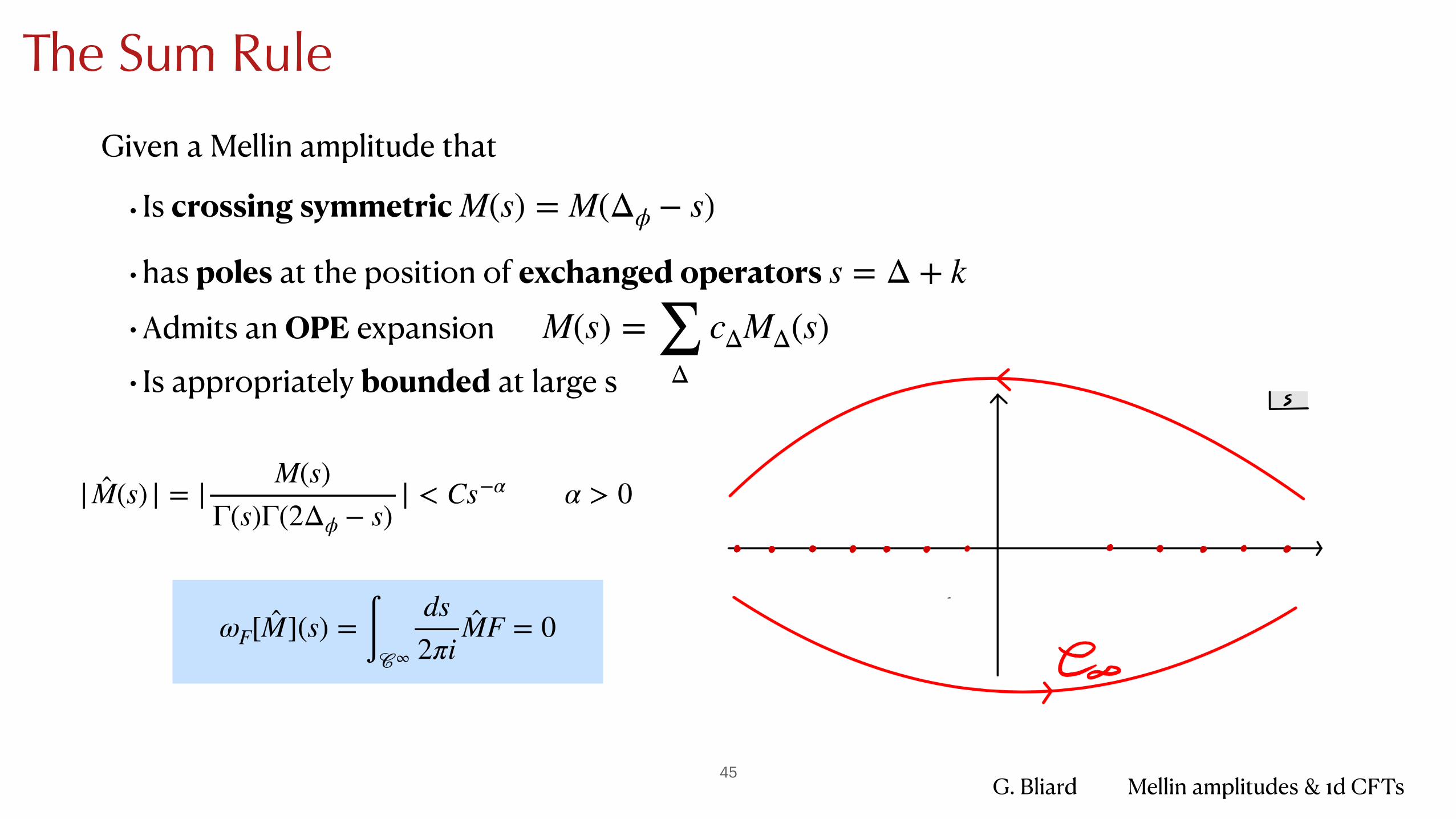
The Sum Rule
Given a Mellin amplitude that
• Is crossing symmetric
• has poles at the position of exchanged operators
• Admits an OPE expansion • Is appropriately bounded at large s
M(s) = M(Δϕ − s)
s = Δ + k
ωF[M̂](s) = ∫𝒞∞
ds2πi
M̂F = 0
|M̂(s) | = |M(s)
Γ(s)Γ(2Δϕ − s)| < Cs−α α > 0
M(s) = ∑Δ
cΔMΔ(s)
46
G. Bliard Mellin amplitudes & 1d CFTs47
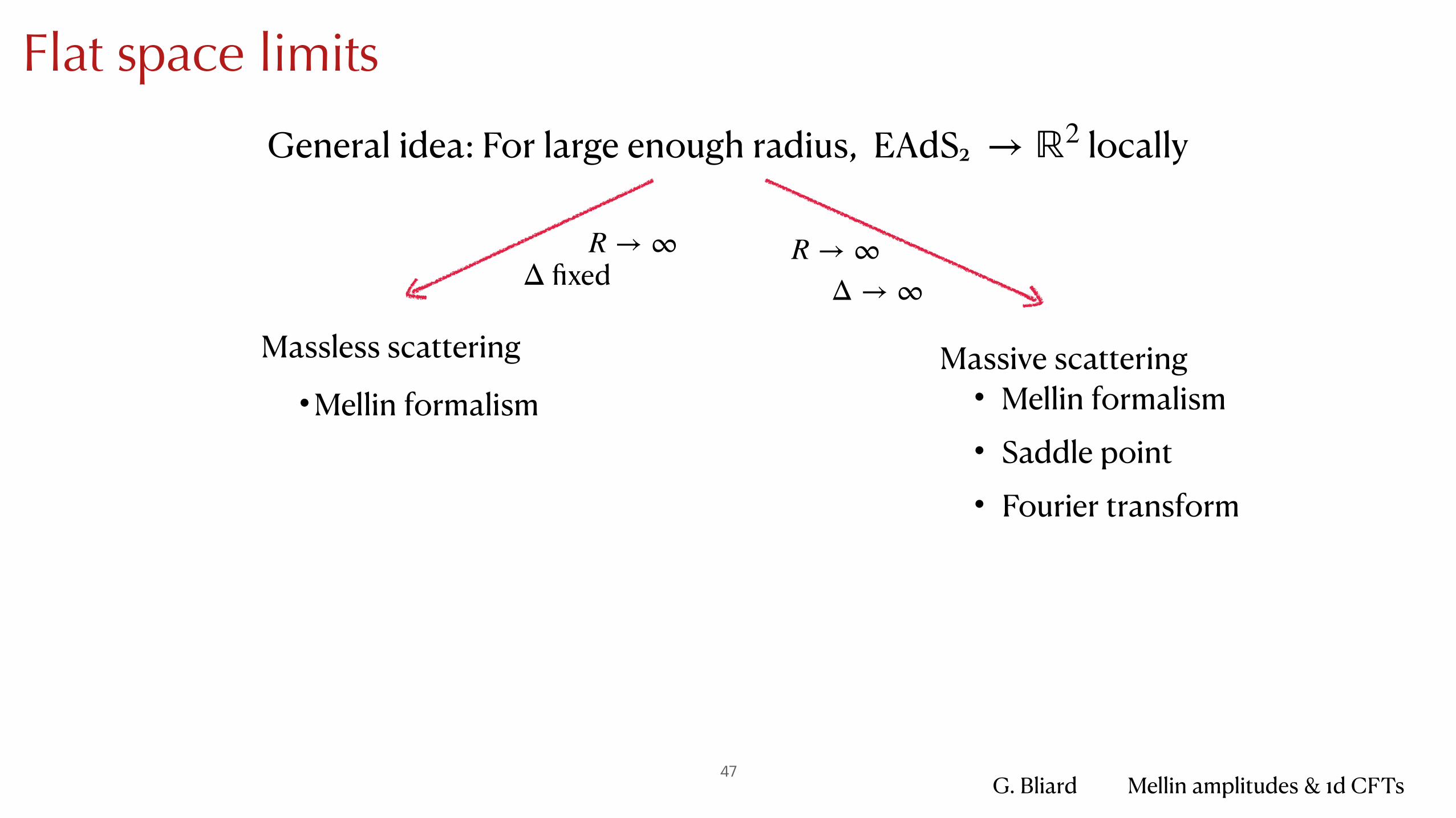
Flat space limits
General idea: For large enough radius, EAdS2 locally→ ℝ2
R → ∞ R → ∞Δ → ∞
Massless scattering Massive scattering • Mellin formalism • Saddle point • Fourier transform
fixedΔ
•Mellin formalism
G. Bliard Mellin amplitudes & 1d CFTs48
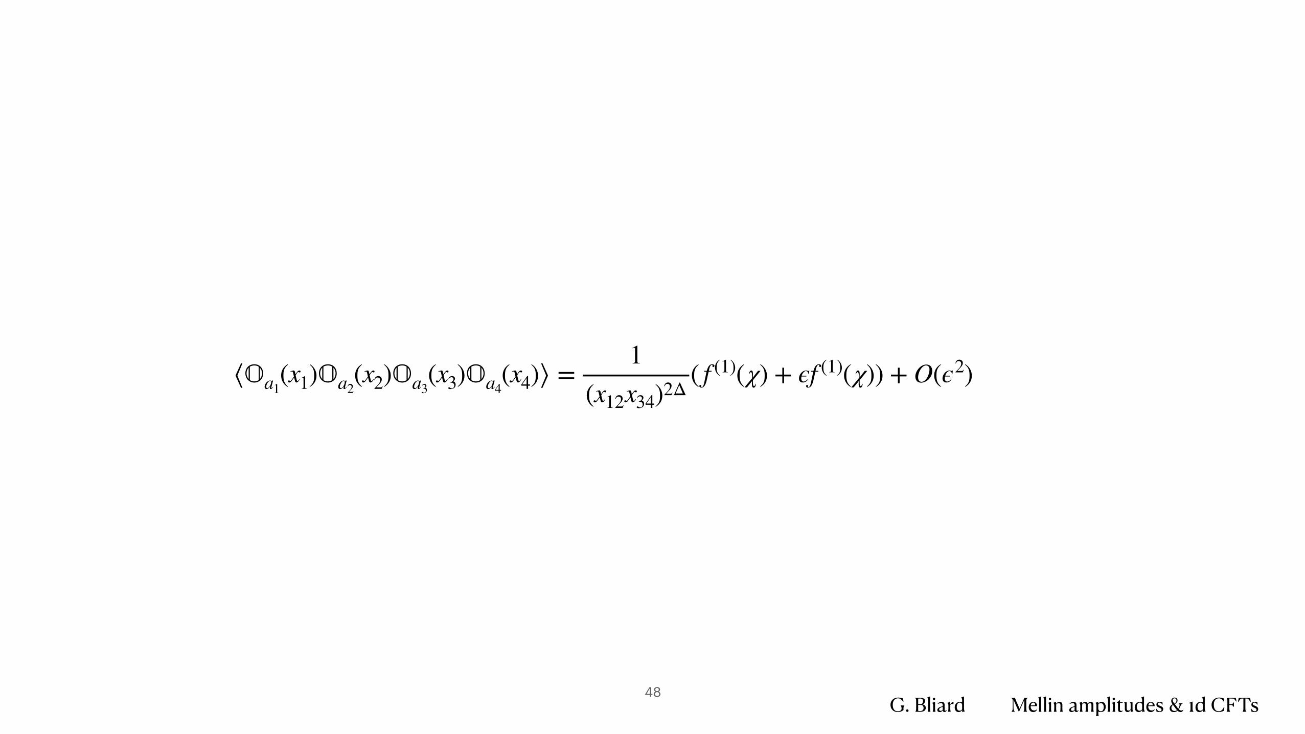
⟨𝕆a1(x1)𝕆a2
(x2)𝕆a3(x3)𝕆a4
(x4)⟩ =1
(x12x34)2Δ( f (1)(χ) + ϵf (1)(χ)) + O(ϵ2)

G. Bliard Mellin amplitudes & 1d CFTs49
How can we study CFT1?
Localisation [Giombi, Komatsu ’18] [Gorini, Griguolo, Guerrini, Penati, Seminara, Soresina ’20]
Mellin amplitudes [Ferrero, Ghosh, Sinha, Zahed ’18]
Analytic Bootstrap [Liendo, Meneghelli, Mitev ’18] [Mazac , Paulos] [Ferrero, Ghosh, Sinha, Zahed ’18]
Integrability [Grabner, Gromov, Julius ’20] [Drukker Kawamoto ’06]
Feynman diagrams
[Cooke, Dekel, Drukker, ’17] [Kyriu, Komatsu ’18] [Barrat, Liendo, Plefka ’20]
Witten diagrams [Giombi, Roiban, Tseytlin ’17]
G. Bliard Mellin amplitudes & 1d CFTs50
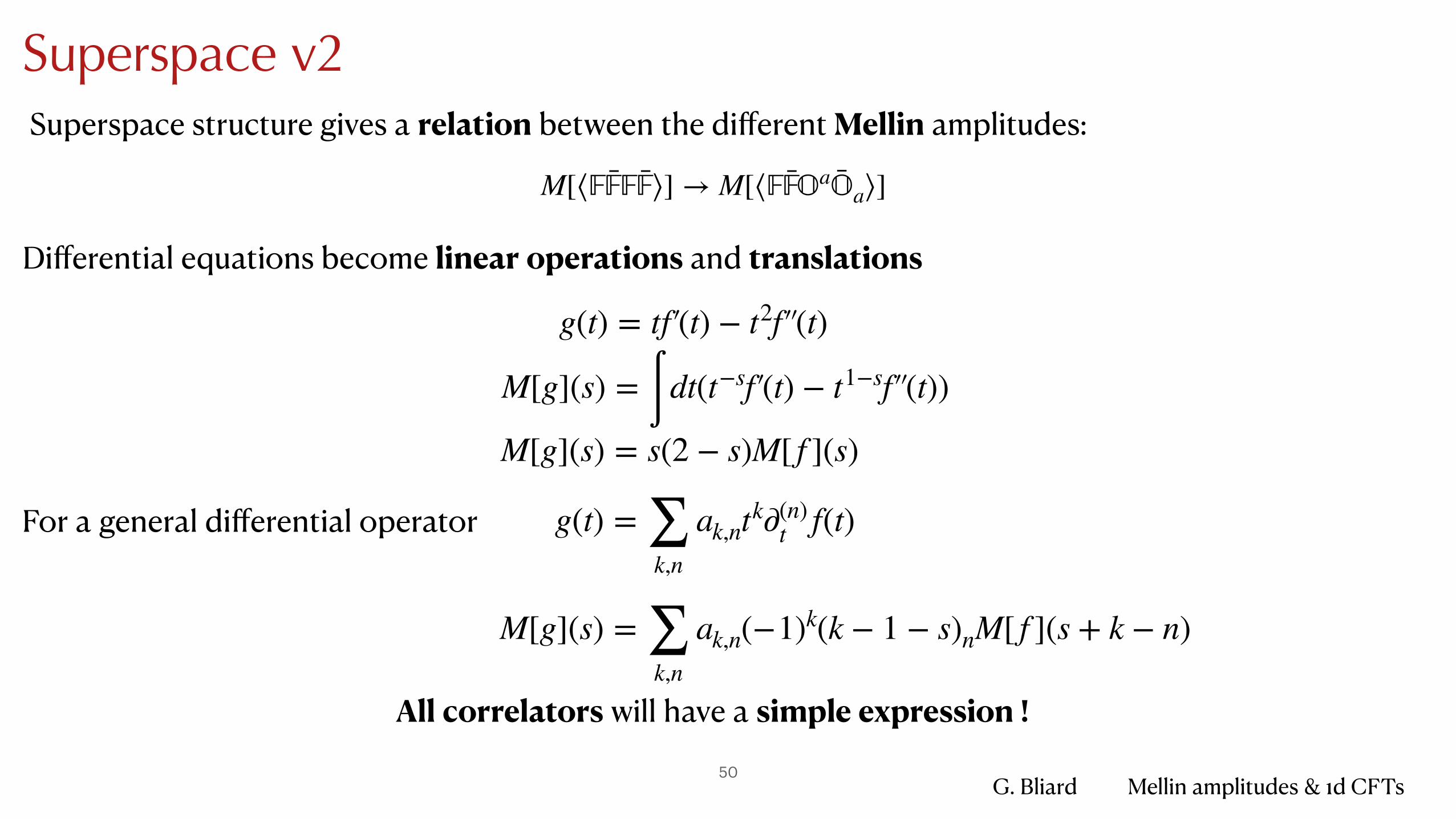
Superspace v2Superspace structure gives a relation between the different Mellin amplitudes:
M[⟨𝔽𝔽𝔽𝔽⟩] → M[⟨𝔽𝔽𝕆a�̄�a⟩]
Differential equations become linear operations and translations
All correlators will have a simple expression !
g(t) = tf′ (t) − t2f′ ′ (t)
M[g](s) = ∫ dt(t−sf′ (t) − t1−sf′ ′ (t))
M[g](s) = s(2 − s)M[ f ](s)
For a general differential operator g(t) = ∑k,n
ak,ntk∂(n)t f(t)
M[g](s) = ∑k,n
ak,n(−1)k(k − 1 − s)nM[ f ](s + k − n)


![arXiv:1107.1504v3 [hep-th] 5 Oct 2011 · 2011. 10. 6. · Preprint typeset in JHEP style - HYPER VERSION Towards Feynman rules for Mellin amplitudes in AdS/CFT Miguel F. Paulosa a](https://img.pdfslide.net/doc/110x75/60c0fcf408f80826ea0b5881/arxiv11071504v3-hep-th-5-oct-2011-2011-10-6-preprint-typeset-in-jhep-style.jpg)


![Recursion Relations in p-adic Mellin Space · Recursion Relations in p-adic Mellin Space ... in the context of p-adic AdS/CFT [2,3] initiated in Ref. [4]. These so-called p-adic Mellin](https://img.pdfslide.net/doc/110x75/5fb887154b41c23cfb6175b2/recursion-relations-in-p-adic-mellin-space-recursion-relations-in-p-adic-mellin.jpg)