Embed Size (px)
Citation preview
1 +Corresponding author; email [email protected], tel. +39 09123863788
A THERMOCHROMIC LIQUID CRYSTALS IMAGE ANALYSIS TECHNIQUE TO
INVESTIGATE TEMPERATURE POLARIZATION IN SPACER-FILLED CHANNELS
FOR MEMBRANE DISTILLATION
A. Tamburini*, P. Pitò*, A. Cipollina*+, G. Micale*, M. Ciofalo**
*Dipartimento di Ingegneria Chimica, Gestionale, Informatica, Meccanica
** Dipartimento dell’Energia, Ingegneria dell'Informazione e Modelli Matematici
Università degli Studi di Palermo, Viale delle Scienze, 90128 Palermo, Italy
ABSTRACT
The analysis of flow fields and temperature distributions is of paramount importance in the
development and optimization of new spacer-filled channel geometries for Membrane Distillation
modules. The literature reports only few studies on the experimental characterization of such
channels and, to the authors’ knowledge, none of them presents local information concerning the
temperature distribution on the membrane surface. In the present work, a non-intrusive
experimental technique named TLC-IA-TP is presented: it is based on the use of Thermochromic
Liquid Crystals (TLCs) and digital Image Analysis (IA) and it is applied here for the first time to
the analysis of Temperature Polarization (TP) in spacer-filled channels typically adopted in
thermally-driven membrane separation processes. In particular, this technique allows the local
distribution of convective heat transfer coefficients to be determined, thus providing (i) useful
indications on strengths and weaknesses of some spacer arrangements and (ii) valuable benchmark
data for Computational Fluid Dynamics (CFD) studies. For the purpose of the present work, the
Cite this article as: Tamburini, A., Pitò, P., Cipollina, A, Micale, G., Ciofalo, M., A Thermochromic Liquid Crystals Image Analysis technique to investigate polarization in spacer-filled channel, Journal of Membrane Science, 447 (2013) 260-273. http://dx.doi.org/10.1016/j.memsci.2013.06.043

2
technique’s fundamentals are presented, along with a comprehensive assessment of the technique’s
accuracy. Results of some preliminary measurements on commercial spacers are also reported.
Keywords: Membrane distillation, Temperature polarization, Thermochromic Liquid Crystals,
Digital Image Analysis, Spacer filled channel
3
1 INTRODUCTION AND LITERATURE REVIEW
Membrane distillation (MD) is a relatively new process that is being investigated worldwide as a
low cost, energy saving alternative to conventional separation processes such as distillation and
reverse osmosis [1,2]. Nowadays, the possibility of driving the process via solar thermal energy and
waste heat has further enhanced the interest towards this technique [3-7]. MD is a separation
technique combining the features of both thermal and membrane-based distillation processes.
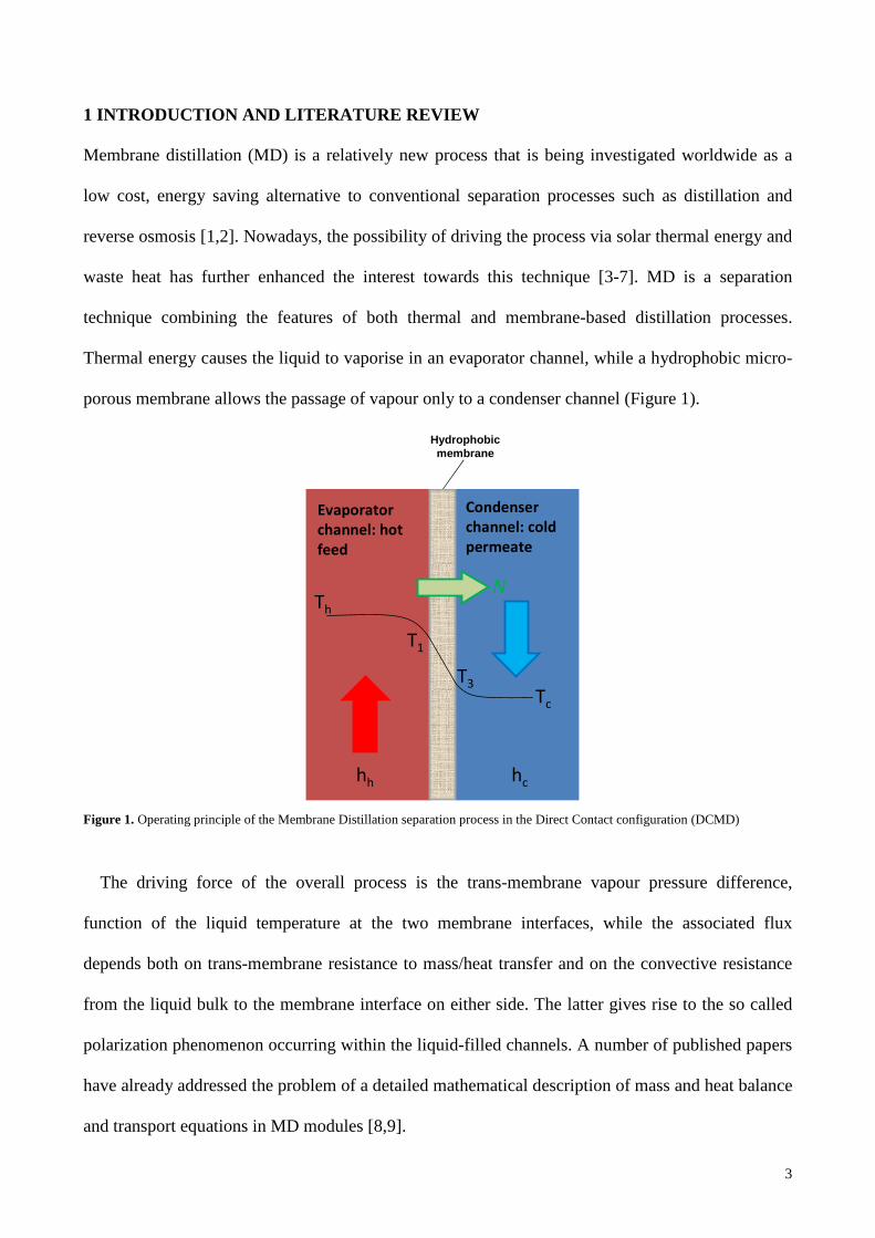
Thermal energy causes the liquid to vaporise in an evaporator channel, while a hydrophobic micro-
porous membrane allows the passage of vapour only to a condenser channel (Figure 1).
Hydrophobic membrane
Th
T1
T3Tc
Evaporator
channel: hot
feed
Condenser
channel: cold
permeate
N
hh hc
Figure 1. Operating principle of the Membrane Distillation separation process in the Direct Contact configuration (DCMD)
The driving force of the overall process is the trans-membrane vapour pressure difference,
function of the liquid temperature at the two membrane interfaces, while the associated flux
depends both on trans-membrane resistance to mass/heat transfer and on the convective resistance
from the liquid bulk to the membrane interface on either side. The latter gives rise to the so called
polarization phenomenon occurring within the liquid-filled channels. A number of published papers
have already addressed the problem of a detailed mathematical description of mass and heat balance
and transport equations in MD modules [8,9].
4
Polarization phenomena may play a fundamental role in controlling mass and heat transfer, thus
affecting the process performance in terms of specific flux per unit surface of membrane.
Polarization is also strictly related to the values of the flux crossing the membrane (the higher the
flux, the larger the corresponding polarization). Thus, while most researchers are mainly working
on the development of improved membranes for MD, the problem of temperature polarization may
become the dominant factor limiting flux enhancement, thus hindering the above efforts.
One of the main solutions proposed to the problem of polarization in membrane-based systems is
the promotion of mixing inside the channels by a suitable choice of the module geometry. Indeed,
hydrodynamics is known to play a crucial role in influencing MD module performance [10]. In this
regard, spacers are normally interposed between consecutive membrane sheets in planar or spiral-
wound modules to mechanically support the membranes; such spacers are also beneficial as mixing
promoters. The benefit of different spacer geometries in reducing polarization phenomena, thus
enhancing the overall performance of the process, may be significant [11]. On the other hand, the
presence of a spacer may significantly influence the fluid flow also in terms of pressure drops and
shear stresses as demonstrated by a number of published studies [12-16]. Spacers so far adopted for
MD applications are basically nets consisting of two or more layers of polymeric wires, which are
often thought of and designed for completely different applications than MD separation. In this
regard a suitable optimization of their features and geometrical configuration would be desirable to
enhance the process performance.
Since mixing enhancement depends, in general, on all the geometrical features of a spacer, the
effect of using different types of spacers in MD channels has been studied in order to find the
geometric characteristics which maximize the heat transfer coefficient and the corresponding mass
flux across the membrane, i.e. minimize the temperature polarization effect [17-21].
Spacers can be characterized by wire diameter, distance between subsequent wires, angle
between wires, wire orientation with respect to the flow, etc.. In particular, the last feature is known
to be one of the most important, as it is responsible for the changes in flow direction and flow
pattern [22,23]. Recently Shakaib et al. (2012) [24] employed Computational Fluid Dynamics
5
(CFD) to address this issue and confirmed that spacer orientation greatly affects temperature
polarization and heat transfer rates.
Phattaranawik et al. [25] measured 30-40% enhancements in mass flux across the membrane in
DCMD when the channel was filled with a spacer with respect to the values obtained with an empty
channel. This occurrence was also associated with a substantial increase of the temperature
polarization coefficient τ, defined as the ratio between the trans-membrane temperature difference
and the difference between bulk temperatures in the two channels: with reference to Figure 1
( ) ( )ch TTTT −−= 31τ (1)
According to this definition, the lower the value of τ, the stronger is the effect of temperature
polarization on the driving force, thus worsening the performance of the separation process. A
coefficient ranging from 0.57 to 0.76 was found for the case of an empty channel, against values
ranging from 0.9 to 0.97 in spacer-filled channels (at the same mass flow rate).
Martìnez and Rodrìguez-Maroto [26] demonstrated how the presence of a spacer significantly
increases not only the heat transfer coefficient but also its dependence on the fluid flow velocity
inside the channel.
Chernyshov et al. [27] carried out experiments on temperature polarization in Air Gap Membrane
Distillation (AGMD) module with the aim of investigating the dependence of permeate flux and
pressure drop on flow rate for five spacers of the same thickness but different geometries. They
obtained fluxes up to 2.5 times higher in spacer-filled channels than that in an empty channel, thus
concluding that employing an empty channel is an unacceptable choice.
Lower enhancements of the permeate flux (up to 30%) were obtained by Yun et al. [28] for the
case of DCMD modules. They also found that the effect of a spacer placed in the hot-side channel
was larger than that of the same spacer placed on the cold-side.
It should be observed that the beneficial effect of the spacer on the overall performance decreases
at high flow rates, when mixing is already promoted by turbulence in the fluid. In this regard, the
6
findings by Phattaranawik et al. [29] suggest the existence of transitional fluid flow within the
spacer-filled channels at typical MD operating conditions.
Another important aspect is the spatial resolution of the experimental techniques adopted so far.
Up to now, most studies have focused on the evaluation of efficiency enhancement at a large scale
by referring only to average values of temperature and heat or mass flux. Surprisingly, only little
attention has been devoted to the local characterization of the spacer influence on the separation
process. Data on temperature distributions would allow a better understanding of temperature
polarization phenomena as related to the spacer’s geometry, thus guiding the choice of the more
effective spacer-channel configurations. CFD may greatly aid the design of improved spacers for
MD processes: a CFD model may intrinsically be able to provide local information on temperature
distribution and polarization as well as on flow field and pressure drops with any level of detail.
Thus, many efforts have been devoted to the CFD simulation of spacer-filled channel modules for
MD [20,21,24,30,31], but the results obtained have not yet been sufficiently validated because of
the lack of detailed experimental information on local temperature and heat transfer coefficient
distributions [32].
This issue is addressed in this work by employing a novel space-resolved technique, briefly
presented in two previous conference papers [33-34] by the same authors, to assess the local
temperature and heat transfer coefficient distribution on the membrane surface. This technique,
named TLC-IA-TP, makes a combined use of Thermochromic Liquid Crystals and digital Image
Analysis.
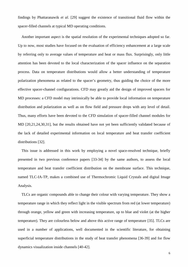
TLCs are organic compounds able to change their colour with varying temperature. They show a
temperature range in which they reflect light in the visible spectrum from red (at lower temperature)
through orange, yellow and green with increasing temperature, up to blue and violet (at the higher
temperature). They are colourless below and above this active range of temperature [35]. TLCs are
used in a number of applications, well documented in the scientific literature, for obtaining
superficial temperature distributions in the study of heat transfer phenomena [36-39] and for flow
dynamics visualization inside channels [40-42].
7
2 EXPERIMENTAL SET-UP AND PROCEDURES
2.1 Description of the experimental facility
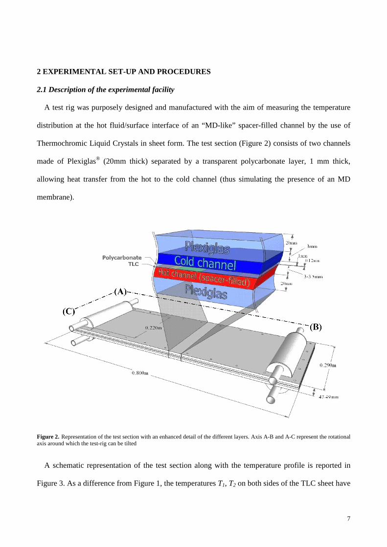
A test rig was purposely designed and manufactured with the aim of measuring the temperature
distribution at the hot fluid/surface interface of an “MD-like” spacer-filled channel by the use of
Thermochromic Liquid Crystals in sheet form. The test section (Figure 2) consists of two channels
made of Plexiglas® (20mm thick) separated by a transparent polycarbonate layer, 1 mm thick,
allowing heat transfer from the hot to the cold channel (thus simulating the presence of an MD
membrane).
Figure 2. Representation of the test section with an enhanced detail of the different layers. Axis A-B and A-C represent the rotational axis around which the test-rig can be tilted
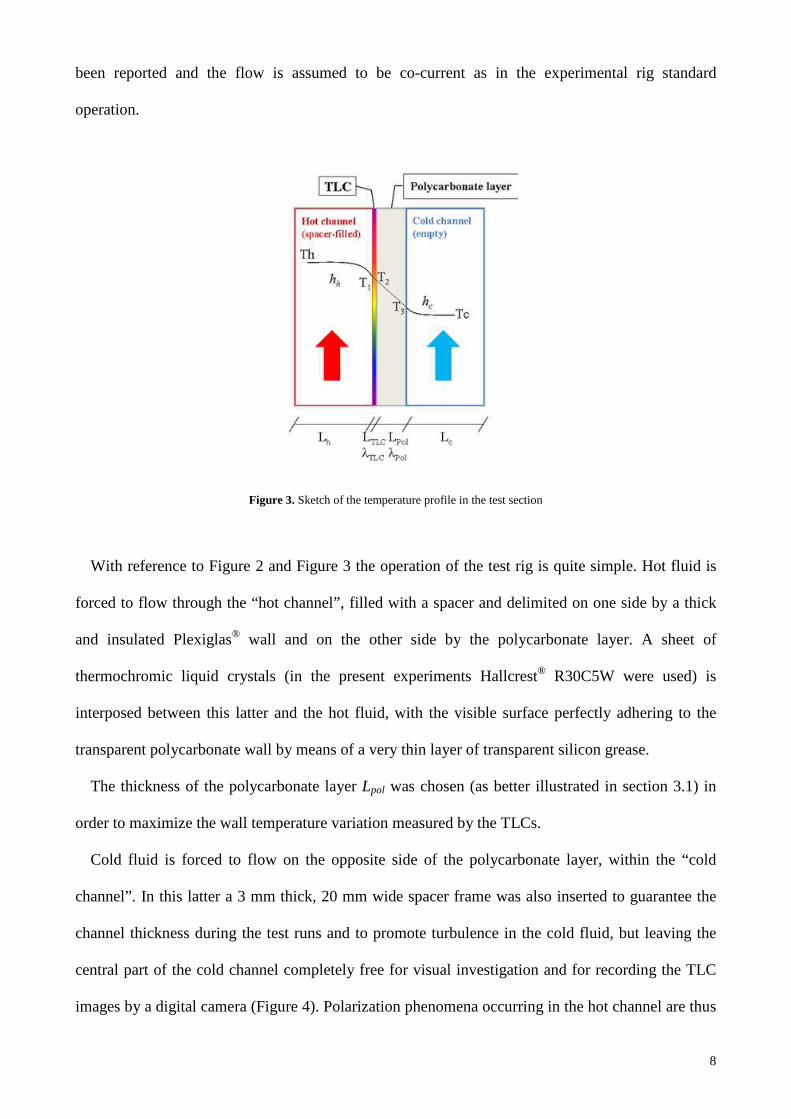
A schematic representation of the test section along with the temperature profile is reported in
Figure 3. As a difference from Figure 1, the temperatures T1, T2 on both sides of the TLC sheet have
8
been reported and the flow is assumed to be co-current as in the experimental rig standard
operation.
Figure 3. Sketch of the temperature profile in the test section
With reference to Figure 2 and Figure 3 the operation of the test rig is quite simple. Hot fluid is
forced to flow through the “hot channel”, filled with a spacer and delimited on one side by a thick
and insulated Plexiglas® wall and on the other side by the polycarbonate layer. A sheet of
thermochromic liquid crystals (in the present experiments Hallcrest® R30C5W were used) is
interposed between this latter and the hot fluid, with the visible surface perfectly adhering to the
transparent polycarbonate wall by means of a very thin layer of transparent silicon grease.
The thickness of the polycarbonate layer Lpol was chosen (as better illustrated in section 3.1) in
order to maximize the wall temperature variation measured by the TLCs.
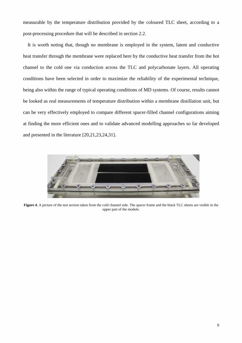
Cold fluid is forced to flow on the opposite side of the polycarbonate layer, within the “cold
channel”. In this latter a 3 mm thick, 20 mm wide spacer frame was also inserted to guarantee the
channel thickness during the test runs and to promote turbulence in the cold fluid, but leaving the
central part of the cold channel completely free for visual investigation and for recording the TLC
images by a digital camera (Figure 4). Polarization phenomena occurring in the hot channel are thus
9
measurable by the temperature distribution provided by the coloured TLC sheet, according to a
post-processing procedure that will be described in section 2.2.
It is worth noting that, though no membrane is employed in the system, latent and conductive
heat transfer through the membrane were replaced here by the conductive heat transfer from the hot
channel to the cold one via conduction across the TLC and polycarbonate layers. All operating
conditions have been selected in order to maximize the reliability of the experimental technique,
being also within the range of typical operating conditions of MD systems. Of course, results cannot
be looked as real measurements of temperature distribution within a membrane distillation unit, but
can be very effectively employed to compare different spacer-filled channel configurations aiming
at finding the more efficient ones and to validate advanced modelling approaches so far developed
and presented in the literature [20,21,23,24,31].
Figure 4. A picture of the test section taken from the cold channel side. The spacer frame and the black TLC sheets are visible in the upper part of the module.
10
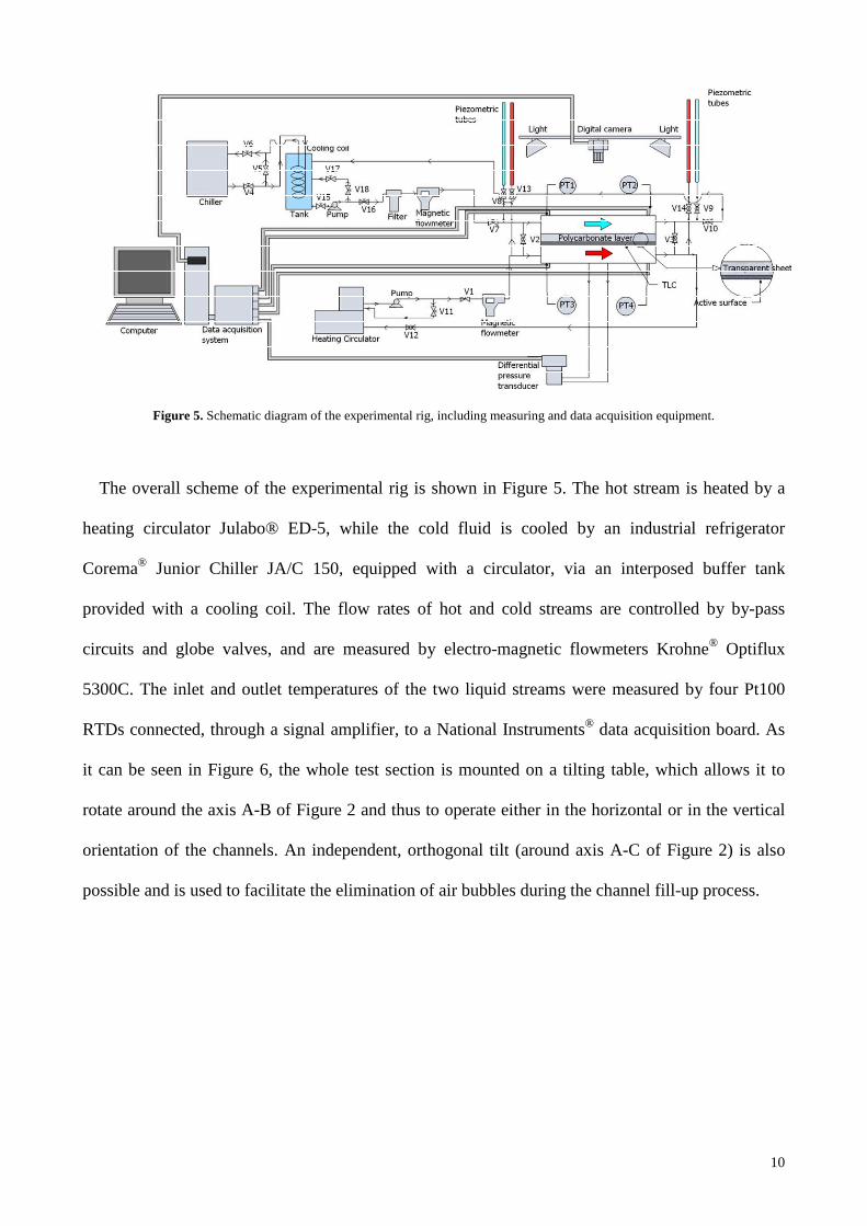
Figure 5. Schematic diagram of the experimental rig, including measuring and data acquisition equipment.
The overall scheme of the experimental rig is shown in Figure 5. The hot stream is heated by a
heating circulator Julabo® ED-5, while the cold fluid is cooled by an industrial refrigerator
Corema® Junior Chiller JA/C 150, equipped with a circulator, via an interposed buffer tank
provided with a cooling coil. The flow rates of hot and cold streams are controlled by by-pass
circuits and globe valves, and are measured by electro-magnetic flowmeters Krohne® Optiflux
5300C. The inlet and outlet temperatures of the two liquid streams were measured by four Pt100
RTDs connected, through a signal amplifier, to a National Instruments® data acquisition board. As
it can be seen in Figure 6, the whole test section is mounted on a tilting table, which allows it to
rotate around the axis A-B of Figure 2 and thus to operate either in the horizontal or in the vertical
orientation of the channels. An independent, orthogonal tilt (around axis A-C of Figure 2) is also
possible and is used to facilitate the elimination of air bubbles during the channel fill-up process.
11
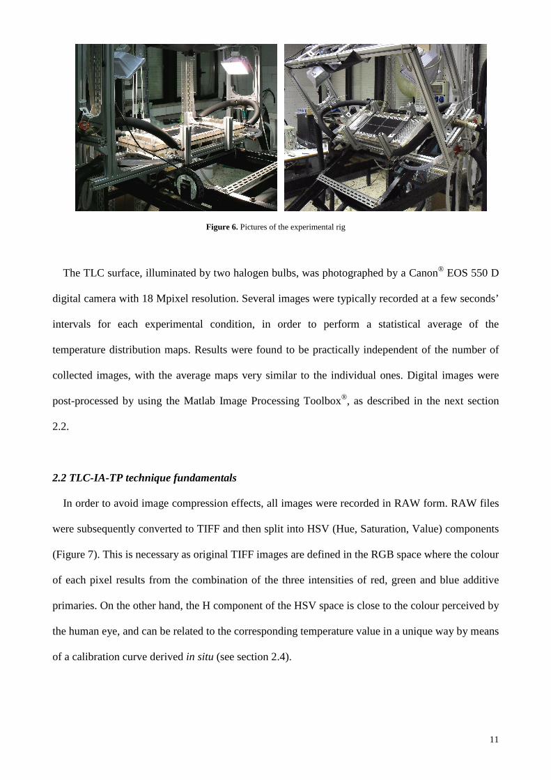
Figure 6. Pictures of the experimental rig
The TLC surface, illuminated by two halogen bulbs, was photographed by a Canon® EOS 550 D
digital camera with 18 Mpixel resolution. Several images were typically recorded at a few seconds’
intervals for each experimental condition, in order to perform a statistical average of the
temperature distribution maps. Results were found to be practically independent of the number of
collected images, with the average maps very similar to the individual ones. Digital images were
post-processed by using the Matlab Image Processing Toolbox®, as described in the next section
2.2.
2.2 TLC-IA-TP technique fundamentals
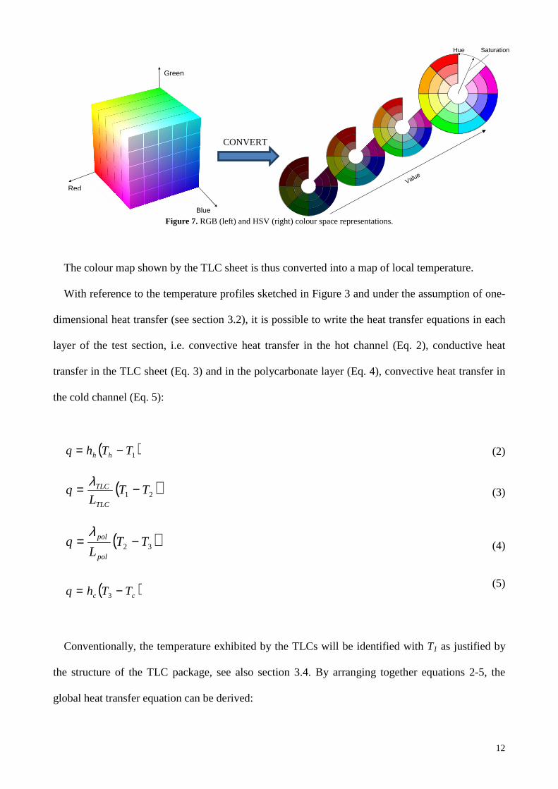
In order to avoid image compression effects, all images were recorded in RAW form. RAW files
were subsequently converted to TIFF and then split into HSV (Hue, Saturation, Value) components
(Figure 7). This is necessary as original TIFF images are defined in the RGB space where the colour
of each pixel results from the combination of the three intensities of red, green and blue additive
primaries. On the other hand, the H component of the HSV space is close to the colour perceived by
the human eye, and can be related to the corresponding temperature value in a unique way by means
of a calibration curve derived in situ (see section 2.4).
12
Red
Blue
Green
Value
Hue Saturation
Figure 7. RGB (left) and HSV (right) colour space representations.
The colour map shown by the TLC sheet is thus converted into a map of local temperature.
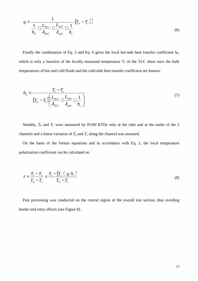
With reference to the temperature profiles sketched in Figure 3 and under the assumption of one-
dimensional heat transfer (see section 3.2), it is possible to write the heat transfer equations in each
layer of the test section, i.e. convective heat transfer in the hot channel (Eq. 2), conductive heat
transfer in the TLC sheet (Eq. 3) and in the polycarbonate layer (Eq. 4), convective heat transfer in
the cold channel (Eq. 5):
( )1TThq hh −= (2)
( )21 TTL
qTLC
TLC −= λ (3)
( )32 TTL
qpol
pol −=λ
(4)
( )cc TThq −= 3
(5)
Conventionally, the temperature exhibited by the TLCs will be identified with T1 as justified by
the structure of the TLC package, see also section 3.4. By arranging together equations 2-5, the
global heat transfer equation can be derived:
CONVERT
13
( )ch
cpol
pol
TLC
TLC
h
TT
h
LL
h
q −+++
=11
1
λλ (6)
Finally the combination of Eq. 2 and Eq. 6 gives the local hot-side heat transfer coefficient hh,
which is only a function of the locally measured temperature T1 of the TLC sheet once the bulk
temperatures of hot and cold fluids and the cold-side heat transfer coefficient are known:
( )
++−
−=
cpol
pol
TLC
TLCh
ch
h
LLTT
TTh
11
1
λλ
(7)
Notably, Th and Tc were measured by Pt100 RTDs only at the inlet and at the outlet of the 2
channels and a linear variation of Th and Tc along the channel was assumed.
On the basis of the former equations and in accordance with Eq. 1, the local temperature
polarization coefficient can be calculated as:
( )ch
cc
ch TT
hqTT
TT
TT
−+−=
−−= 131τ (8)
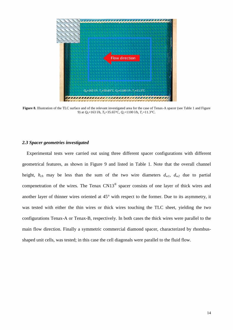
Post processing was conducted on the central region of the overall test section, thus avoiding
border and entry effects (see Figure 8).
14
Figure 8. Illustration of the TLC surface and of the relevant investigated area for the case of Tenax-A spacer (see Table 1 and Figure 9) at Qh=163 l/h, Th=35.65°C, Qc=1100 l/h, Tc=11.3°C.
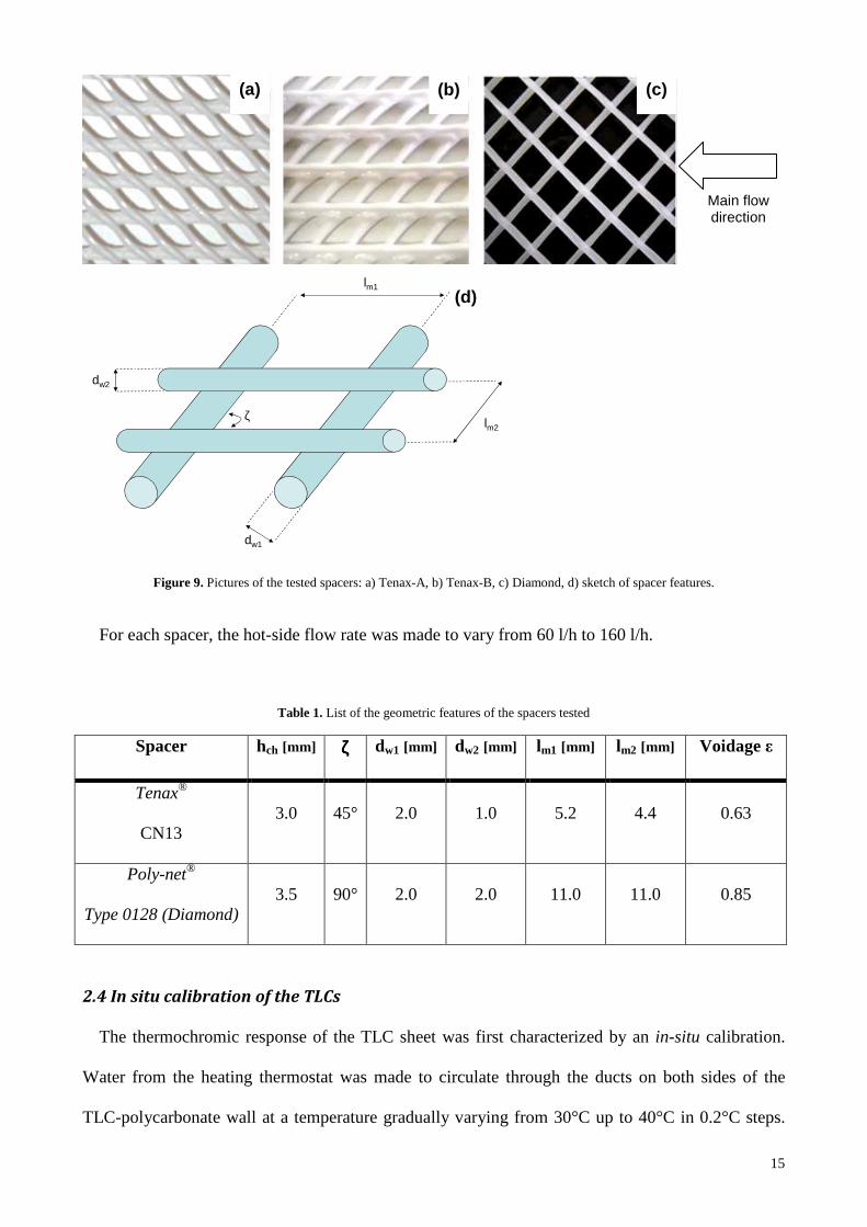
2.3 Spacer geometries investigated
Experimental tests were carried out using three different spacer configurations with different
geometrical features, as shown in Figure 9 and listed in Table 1. Note that the overall channel
height, hch may be less than the sum of the two wire diameters dw1, dw2 due to partial
compenetration of the wires. The Tenax CN13® spacer consists of one layer of thick wires and
another layer of thinner wires oriented at 45° with respect to the former. Due to its asymmetry, it
was tested with either the thin wires or thick wires touching the TLC sheet, yielding the two
configurations Tenax-A or Tenax-B, respectively. In both cases the thick wires were parallel to the
main flow direction. Finally a symmetric commercial diamond spacer, characterized by rhombus-
shaped unit cells, was tested; in this case the cell diagonals were parallel to the fluid flow.
15
Figure 9. Pictures of the tested spacers: a) Tenax-A, b) Tenax-B, c) Diamond, d) sketch of spacer features.
For each spacer, the hot-side flow rate was made to vary from 60 l/h to 160 l/h.
Table 1. List of the geometric features of the spacers tested
Spacer hch [mm] ζζζζ dw1 [mm] dw2 [mm] lm1 [mm] lm2 [mm] Voidage ε
Tenax®
CN13 3.0 45° 2.0 1.0 5.2 4.4 0.63
Poly-net®
Type 0128 (Diamond) 3.5 90° 2.0 2.0 11.0 11.0 0.85
2.4 In situ calibration of the TLCs
The thermochromic response of the TLC sheet was first characterized by an in-situ calibration.
Water from the heating thermostat was made to circulate through the ducts on both sides of the
TLC-polycarbonate wall at a temperature gradually varying from 30°C up to 40°C in 0.2°C steps.
(d)
dw1
lm1
lm2ζ
dw2
Main flow direction
(a) (b) (c)
16
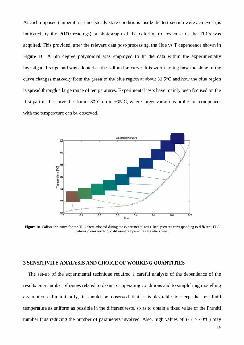
At each imposed temperature, once steady state conditions inside the test section were achieved (as
indicated by the Pt100 readings), a photograph of the colorimetric response of the TLCs was
acquired. This provided, after the relevant data post-processing, the Hue vs T dependence shown in
Figure 10. A 6th degree polynomial was employed to fit the data within the experimentally
investigated range and was adopted as the calibration curve. It is worth noting how the slope of the
curve changes markedly from the green to the blue region at about 31.5°C and how the blue region
is spread through a large range of temperatures. Experimental tests have mainly been focused on the
first part of the curve, i.e. from ~30°C up to ~35°C, where larger variations in the hue component
with the temperature can be observed.
Figure 10. Calibration curve for the TLC sheet adopted during the experimental tests. Real pictures corresponding to different TLC colours corresponding to different temperatures are also shown
3 SENSITIVITY ANALYSIS AND CHOICE OF WORKING QUANTITIES
The set-up of the experimental technique required a careful analysis of the dependence of the
results on a number of issues related to design or operating conditions and to simplifying modelling
assumptions. Preliminarily, it should be observed that it is desirable to keep the hot fluid
temperature as uniform as possible in the different tests, so as to obtain a fixed value of the Prandtl
number thus reducing the number of parameters involved. Also, high values of Th ( > 40°C) may
17
affect the TLCs’ response or even damage them. The value Th = 35°C was chosen in the present
tests. In its turn, the cold fluid bulk temperature Tc could not be reduced too much due to the
limitations of the cooling system. The value Tc = 15°C was adopted here. Finally, in order to
minimize thermal losses and improve the temporal stability, it is desirable that the average system
temperature (Th + Tc)/2 be not too far from the ambient temperature (it was 25°C in the present
tests).
In this section four issues are addressed, namely:
1) the choice of the polycarbonate layer thickness, Lpol;
2) the assumption of one-dimensional heat flux;
3) the accuracy of the heat transfer coefficient estimate within the “cold channel”, hc;
4) the measurement uncertainty.
3.1 Choice of the polycarbonate layer thickness Lpol
Characterizing the dependence of the T1 temperature distribution (recorded by the TLCs) on the
thickness of the polycarbonate layer, Lpol , was an important step in the design of the test section. In
fact, matching the temperature variation of the TLCs with their colour play (range of temperature in
which TLCs are active) allows the resolution of the experimental information collected to be
maximized.
This analysis must be based on the values of the expected heat transfer coefficient in the hot
channel, hh. In particular, the variation range of T1 (Figure 3) corresponding to hh varying from a
minimum hh,min to a maximum hh,max is a function of Lpol and, in some cases, attains a maximum for
a specific value of Lpol as demonstrated in the following.
With reference to the sketch reported in Figure 3, a reduced temperature θ can be defined as:
3TT −=θ (9)
Thus, Eqs. 2 to 4 can be rewritten as:
18
( )1θθ −= hhhq (10)
( )21 θθλ −=TLC
TLC
Lq (11)
2θλ
pol
pol
Lq = (12)
By combining Eqs 11 and 12:
1*
1
1 θθ
λλ
h
pol
pol
TLC
TLC
hLL
q =
+
= (13)
where hh* is a fictitious heat transfer coefficient taking into account for the conduction through
the TLC and polycarbonate layers. By equating Eq. 13 with Eq. 10, the relation between the
temperature θ1 and the polycarbonate layer thickness can be obtained:
*1hh
hh
hh
h
+= θθ (14)
By defining ∆θ as the difference between the values of θ1 calculated for hh = hh,max and hh =
hh,min, it is possible to analyse the trend of ∆θ as a function of Lpol.
This is shown in Figure 11 for Th = 35°C, T3 = 15°C, LTLC = 0.12mm (commercial TLC sheet
thickness), λTLC = 0.15 W/mK, λpol = 0.19 W/mK, hh,min = 400 W/m2K (roughly corresponding to
the thermal conduction through a half channel thickness) and three different values of hh,max (1000,
2500 and 5000 W/m2K).
19
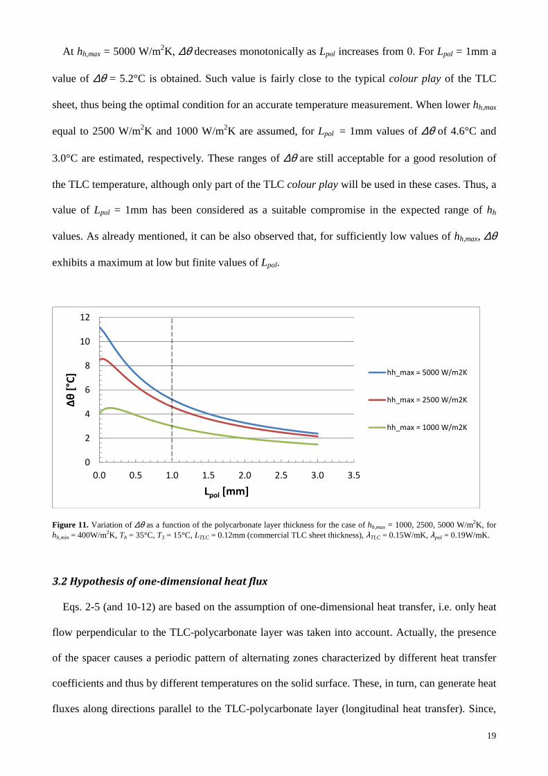
At hh,max = 5000 W/m2K, ∆θ decreases monotonically as Lpol increases from 0. For Lpol = 1mm a
value of ∆θ = 5.2°C is obtained. Such value is fairly close to the typical colour play of the TLC
sheet, thus being the optimal condition for an accurate temperature measurement. When lower hh,max
equal to 2500 W/m2K and 1000 W/m2K are assumed, for Lpol = 1mm values of ∆θ of 4.6°C and
3.0°C are estimated, respectively. These ranges of ∆θ are still acceptable for a good resolution of
the TLC temperature, although only part of the TLC colour play will be used in these cases. Thus, a
value of Lpol = 1mm has been considered as a suitable compromise in the expected range of hh
values. As already mentioned, it can be also observed that, for sufficiently low values of hh,max, ∆θ
exhibits a maximum at low but finite values of Lpol.
0
2
4
6
8
10
12
0.0 0.5 1.0 1.5 2.0 2.5 3.0 3.5
Δθ
[°C
]
Lpol [mm]
hh_max = 5000 W/m2K
hh_max = 2500 W/m2K
hh_max = 1000 W/m2K
Figure 11. Variation of ∆θ as a function of the polycarbonate layer thickness for the case of hh,max = 1000, 2500, 5000 W/m2K, for hh,min = 400W/m2K, Th = 35°C, T3 = 15°C, LTLC = 0.12mm (commercial TLC sheet thickness), λTLC = 0.15W/mK, λpol = 0.19W/mK.
3.2 Hypothesis of one-dimensional heat flux
Eqs. 2-5 (and 10-12) are based on the assumption of one-dimensional heat transfer, i.e. only heat
flow perpendicular to the TLC-polycarbonate layer was taken into account. Actually, the presence
of the spacer causes a periodic pattern of alternating zones characterized by different heat transfer
coefficients and thus by different temperatures on the solid surface. These, in turn, can generate heat
fluxes along directions parallel to the TLC-polycarbonate layer (longitudinal heat transfer). Since,
20
the size of the spacer mesh may be comparable with the thickness of this layer, longitudinal heat
transfer cannot be neglected a priori, and the one-dimensional approximation needs to be validated.
In the following, a simple theoretical analysis, based on the assumption of two-dimensional heat
flux, will be conducted and the corresponding results will be compared with those obtained under
the assumption of one-dimensional heat flux.
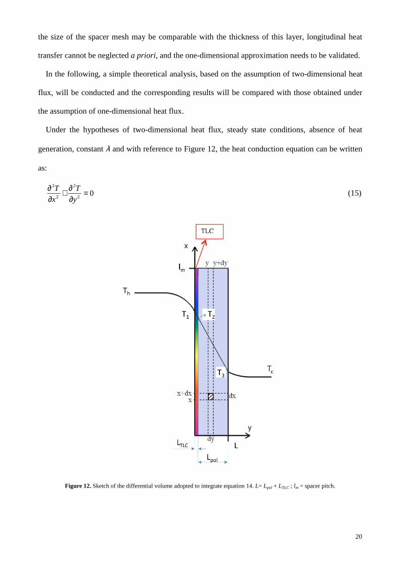
Under the hypotheses of two-dimensional heat flux, steady state conditions, absence of heat
generation, constant λ and with reference to Figure 12, the heat conduction equation can be written
as:
02
2
2
2
=∂∂+
∂∂
y
T
x
T (15)
Figure 12. Sketch of the differential volume adopted to integrate equation 14. L= Lpol + LTLC ; lm = spacer pitch.
21
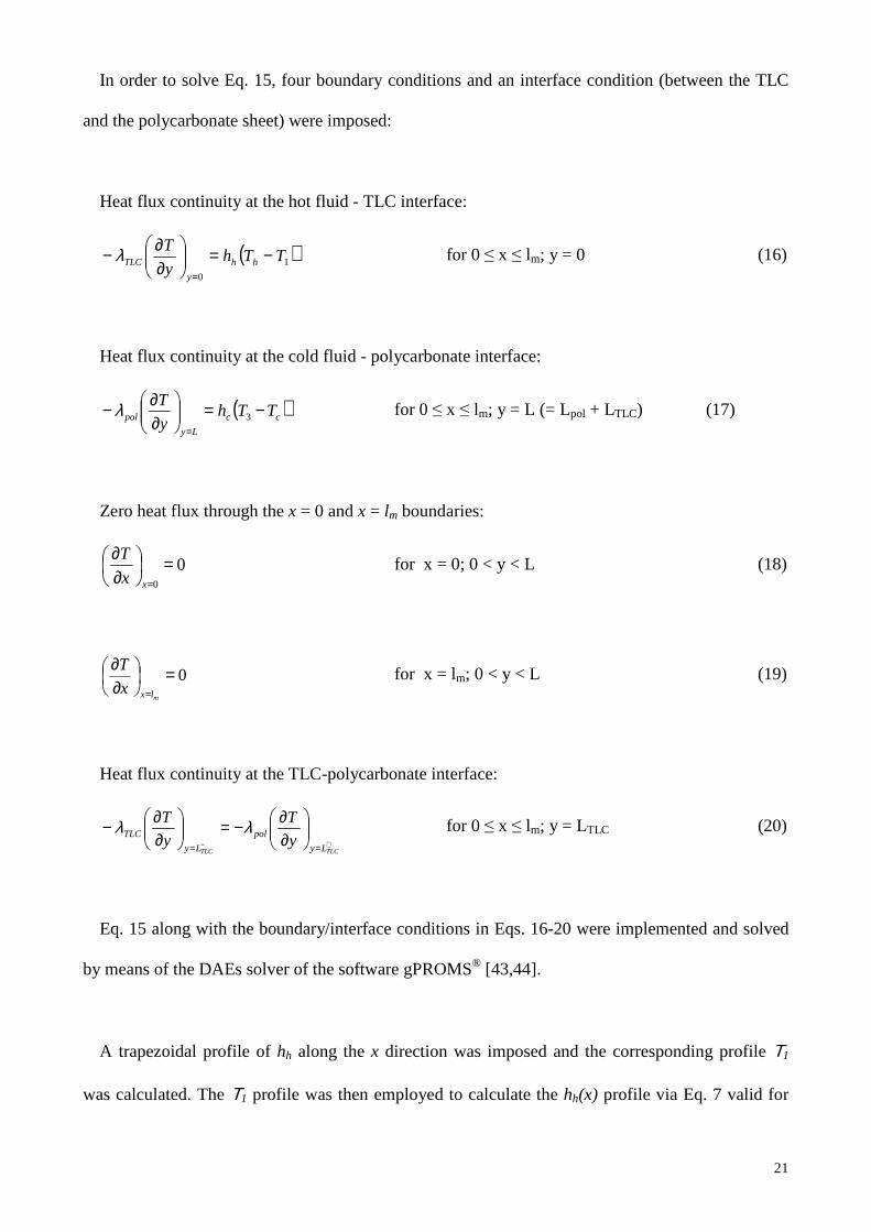
In order to solve Eq. 15, four boundary conditions and an interface condition (between the TLC
and the polycarbonate sheet) were imposed:
Heat flux continuity at the hot fluid - TLC interface:
( )1
0
TThy
Thh
y
TLC −=
∂∂−
=
λ for 0 ≤ x ≤ lm; y = 0 (16)
Heat flux continuity at the cold fluid - polycarbonate interface:
( )cc
Ly
pol TThy
T −=
∂∂−
=3λ for 0 ≤ x ≤ lm; y = L (= Lpol + LTLC) (17)
Zero heat flux through the x = 0 and x = lm boundaries:
00
=
∂∂
=xx
T for x = 0; 0 < y < L (18)
0=
∂∂
= mlxx
T for x = lm; 0 < y < L (19)
Heat flux continuity at the TLC-polycarbonate interface:
+− ==
∂∂−=
∂∂−
TLCTLC Ly
pol
Ly
TLC y
T
y
T λλ for 0 ≤ x ≤ lm; y = LTLC (20)
Eq. 15 along with the boundary/interface conditions in Eqs. 16-20 were implemented and solved
by means of the DAEs solver of the software gPROMS® [43,44].
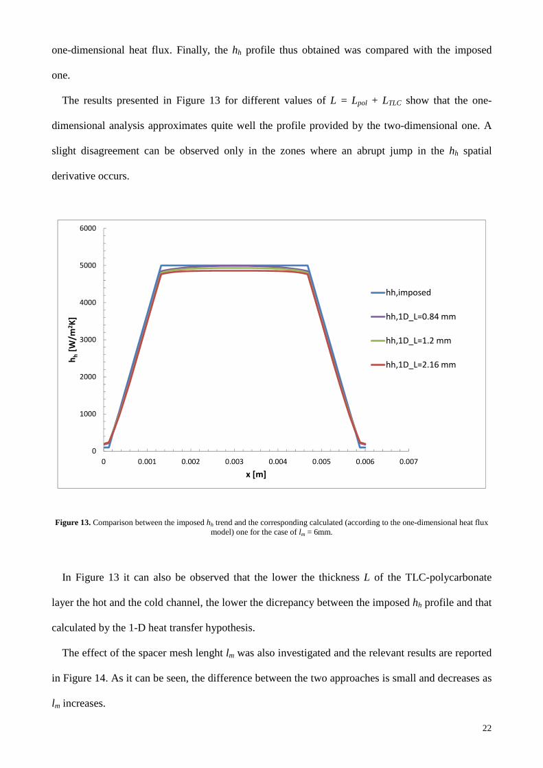
A trapezoidal profile of hh along the x direction was imposed and the corresponding profile Τ1
was calculated. The Τ1 profile was then employed to calculate the hh(x) profile via Eq. 7 valid for
22
one-dimensional heat flux. Finally, the hh profile thus obtained was compared with the imposed
one.
The results presented in Figure 13 for different values of L = Lpol + LTLC show that the one-
dimensional analysis approximates quite well the profile provided by the two-dimensional one. A
slight disagreement can be observed only in the zones where an abrupt jump in the hh spatial
derivative occurs.
0
1000
2000
3000
4000
5000
6000
0 0.001 0.002 0.003 0.004 0.005 0.006 0.007
hh
[W/m
2K
]
x [m]
hh,imposed
hh,1D_L=0.84 mm
hh,1D_L=1.2 mm
hh,1D_L=2.16 mm
Figure 13. Comparison between the imposed hh trend and the corresponding calculated (according to the one-dimensional heat flux model) one for the case of lm = 6mm.
In Figure 13 it can also be observed that the lower the thickness L of the TLC-polycarbonate
layer the hot and the cold channel, the lower the dicrepancy between the imposed hh profile and that
calculated by the 1-D heat transfer hypothesis.
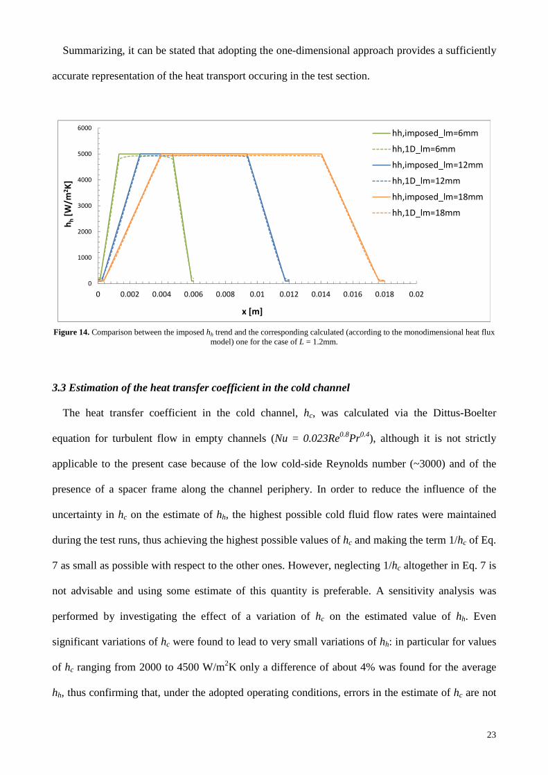
The effect of the spacer mesh lenght lm was also investigated and the relevant results are reported
in Figure 14. As it can be seen, the difference between the two approaches is small and decreases as
lm increases.
23
Summarizing, it can be stated that adopting the one-dimensional approach provides a sufficiently
accurate representation of the heat transport occuring in the test section.
0
1000
2000
3000
4000
5000
6000
0 0.002 0.004 0.006 0.008 0.01 0.012 0.014 0.016 0.018 0.02
hh
[W/m
2K
]
x [m]
hh,imposed_lm=6mm
hh,1D_lm=6mm
hh,imposed_lm=12mm
hh,1D_lm=12mm
hh,imposed_lm=18mm
hh,1D_lm=18mm
Figure 14. Comparison between the imposed hh trend and the corresponding calculated (according to the monodimensional heat flux model) one for the case of L = 1.2mm.
3.3 Estimation of the heat transfer coefficient in the cold channel
The heat transfer coefficient in the cold channel, hc, was calculated via the Dittus-Boelter
equation for turbulent flow in empty channels (Nu = 0.023Re0.8Pr0.4), although it is not strictly
applicable to the present case because of the low cold-side Reynolds number (~3000) and of the
presence of a spacer frame along the channel periphery. In order to reduce the influence of the
uncertainty in hc on the estimate of hh, the highest possible cold fluid flow rates were maintained
during the test runs, thus achieving the highest possible values of hc and making the term 1/hc of Eq.
7 as small as possible with respect to the other ones. However, neglecting 1/hc altogether in Eq. 7 is
not advisable and using some estimate of this quantity is preferable. A sensitivity analysis was
performed by investigating the effect of a variation of hc on the estimated value of hh. Even
significant variations of hc were found to lead to very small variations of hh: in particular for values
of hc ranging from 2000 to 4500 W/m2K only a difference of about 4% was found for the average
hh, thus confirming that, under the adopted operating conditions, errors in the estimate of hc are not
24
significantly detrimental to the accuracy of the hh estimate. Notably, a nominal value of hc ≈ 3000
W/m2K was assumed for the uncertainty assessment presented in the following section.
3.4 Uncertainty assessment
A thorough assessment of the TLC-IA-TP technique uncertainty in estimating hh was carried out
by referring to the uncertainty definition given by Moffat [45]. According to Eq. 7, hh is depending
on n = 8 different quantities “xi”. In formulae: hh = f(T1, Tc, Th, LTLC, λTLC, Lpol, λpol, hc) = f(x1, x2,
… , xn). The uncertainty (standard deviation) of hh can be estimated as:
( ) ( )∑=
∂∂=
n
ii
i
hh x
x
hh
1
2
σσ (21)
Therefore, the assessment of the TLC-IA-TP technique uncertainty requires the knowledge of the
specific uncertainties σ(xi) relevant to each of the xi:
T1) The uncertainty relevant to the temperature of the TLC sheet comes from the calibration
procedure: the conversion from Hue to temperature requires (i) the measurement of the temperature
via Pt100 and (ii) the fitting of the Hue vs T points with a polynomial function. The σ of the Pt100
adopted is 0.05°C (as declared by the manufacturer), while a σ of 0.1°C was found for the fitting.
Thus, the global σ relevant to the variable T1 can be conservatively estimated as 0.15°C. The error
arising by the Hue measurement via the photo-camera and the discretization error (1/256)
associated with the 1-byte representation of Hue are small and were neglected. Notably, the
calibration in situ reduces further possible uncertainties in the estimate of T1, such as those related
with the spectral content of the light source.
Th, Tc) Also the σ relevant to these variables derive from two contributions: one is again due to
the Pt100 uncertainty (i.e. 0.05°C), while the other is due to the assumption of a linear variation of
25
the temperature along the channel. This latter σ was estimated to be 0.1°C. Therefore, the global σ
relevant to the variables Th and Tc has been assumed to be conservatively ~0.15°C.
LTLC, Lpol) For these two quantities a conservative uncertainty of 10-5m was chosen in accordance
with the maximum variability experimentally measured by a thickness gauge (Schimdt Control
Instruments, resolution ± 1 µm) on several samples of TLC and polycarbonate.
λpol) On the basis of the values which can be found in different handbooks, a σ(λpol) equal to
0.015 W/mK was assumed.
λTLC) Since the TLCs are a composite material a σ(λTLC) twice σ(λpol) was chosen.
hc) For the case of the heat transfer coefficient in the cold channel an uncertainty of 500W/m2K
was assumed.
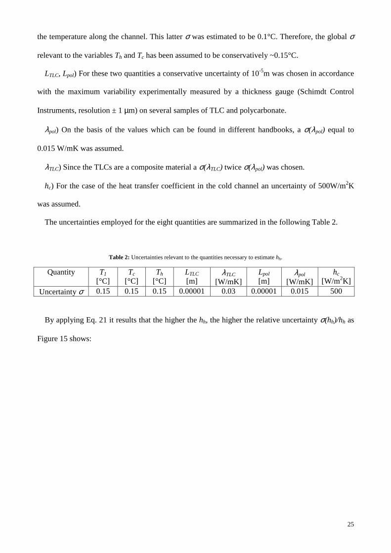
The uncertainties employed for the eight quantities are summarized in the following Table 2.
Table 2: Uncertainties relevant to the quantities necessary to estimate hh.
Quantity T1 [°C]
Tc [°C]
Th [°C]
LTLC [m]
λTLC [W/mK]
Lpol [m]
λpol [W/mK]
hc [W/m2K]
Uncertainty σ 0.15 0.15 0.15 0.00001 0.03 0.00001 0.015 500
By applying Eq. 21 it results that the higher the hh, the higher the relative uncertainty σ(hh)/hh as
Figure 15 shows:
26
0.00
0.05
0.10
0.15
0.20
0.25
0.30
0 500 1000 1500 2000 2500 3000 3500
Re
lati
ve
un
cert
ain
ty o
n h
h[-
]
hh [W/m2K]
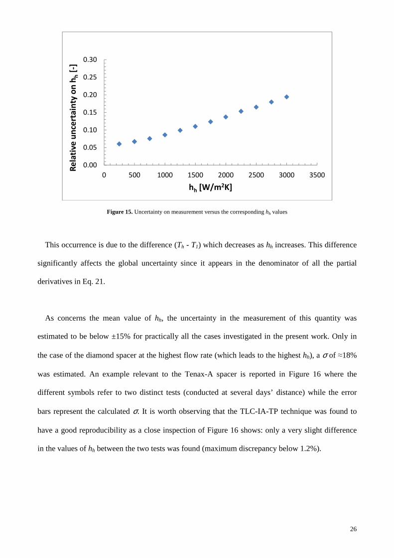
Figure 15. Uncertainty on measurement versus the corresponding hh values
This occurrence is due to the difference (Th - T1) which decreases as hh increases. This difference
significantly affects the global uncertainty since it appears in the denominator of all the partial
derivatives in Eq. 21.
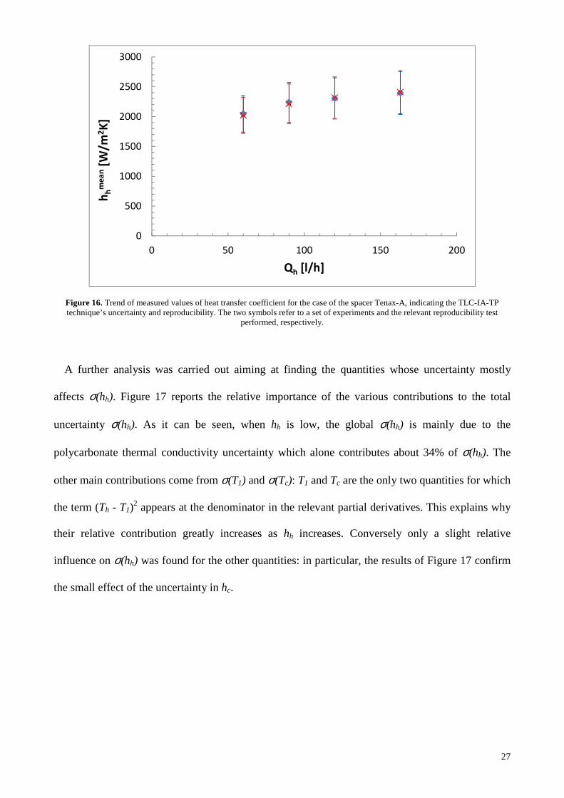
As concerns the mean value of hh, the uncertainty in the measurement of this quantity was
estimated to be below ±15% for practically all the cases investigated in the present work. Only in
the case of the diamond spacer at the highest flow rate (which leads to the highest hh), a σ of ≈18%
was estimated. An example relevant to the Tenax-A spacer is reported in Figure 16 where the
different symbols refer to two distinct tests (conducted at several days’ distance) while the error
bars represent the calculated σ. It is worth observing that the TLC-IA-TP technique was found to
have a good reproducibility as a close inspection of Figure 16 shows: only a very slight difference
in the values of hh between the two tests was found (maximum discrepancy below 1.2%).
27
0
500
1000
1500
2000
2500
3000
0 50 100 150 200
hh
me
an
[W/m
2K
]
Qh [l/h]
Figure 16. Trend of measured values of heat transfer coefficient for the case of the spacer Tenax-A, indicating the TLC-IA-TP technique’s uncertainty and reproducibility. The two symbols refer to a set of experiments and the relevant reproducibility test
performed, respectively.
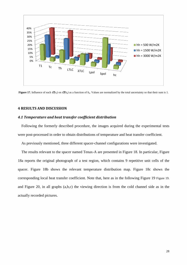
A further analysis was carried out aiming at finding the quantities whose uncertainty mostly
affects σ(hh). Figure 17 reports the relative importance of the various contributions to the total
uncertainty σ(hh). As it can be seen, when hh is low, the global σ(hh) is mainly due to the
polycarbonate thermal conductivity uncertainty which alone contributes about 34% of σ(hh). The
other main contributions come from σ(T1) and σ(Tc): T1 and Tc are the only two quantities for which
the term (Th - T1)2 appears at the denominator in the relevant partial derivatives. This explains why
their relative contribution greatly increases as hh increases. Conversely only a slight relative
influence on σ(hh) was found for the other quantities: in particular, the results of Figure 17 confirm
the small effect of the uncertainty in hc.
28
0%
5%
10%
15%
20%
25%
30%
35%
40%
T1 Tc Th LTLC λTLC Lpol λpol hc
hh = 500 W/m2K
hh = 1500 W/m2K
hh = 3000 W/m2K
Figure 17. Influence of each σ(xi) on σ(hh) as a function of hh. Values are normalized by the total uncertainty so that their sum is 1.
4 RESULTS AND DISCUSSION
4.1 Temperature and heat transfer coefficient distribution
Following the formerly described procedure, the images acquired during the experimental tests
were post-processed in order to obtain distributions of temperature and heat transfer coefficient.
As previously mentioned, three different spacer-channel configurations were investigated.
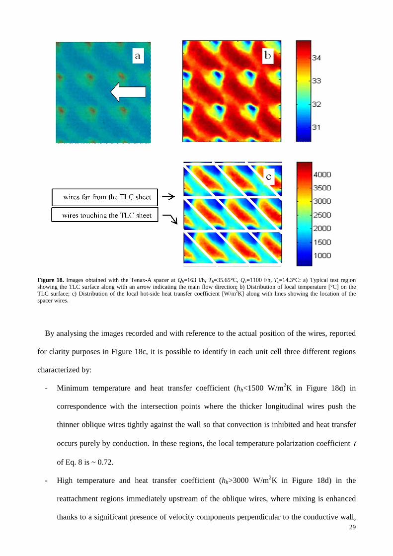
The results relevant to the spacer named Tenax-A are presented in Figure 18. In particular, Figure
18a reports the original photograph of a test region, which contains 9 repetitive unit cells of the
spacer. Figure 18b shows the relevant temperature distribution map. Figure 18c shows the
corresponding local heat transfer coefficient. Note that, here as in the following Figure 19 Figure 19.
and Figure 20, in all graphs (a,b,c) the viewing direction is from the cold channel side as in the
actually recorded pictures.
29
Figure 18. Images obtained with the Tenax-A spacer at Qh=163 l/h, Th=35.65°C, Qc=1100 l/h, Tc=14.3°C: a) Typical test region showing the TLC surface along with an arrow indicating the main flow direction; b) Distribution of local temperature [°C] on the TLC surface; c) Distribution of the local hot-side heat transfer coefficient [W/m2K] along with lines showing the location of the spacer wires.
By analysing the images recorded and with reference to the actual position of the wires, reported
for clarity purposes in Figure 18c, it is possible to identify in each unit cell three different regions
characterized by:
- Minimum temperature and heat transfer coefficient (hh<1500 W/m2K in Figure 18d) in
correspondence with the intersection points where the thicker longitudinal wires push the
thinner oblique wires tightly against the wall so that convection is inhibited and heat transfer
occurs purely by conduction. In these regions, the local temperature polarization coefficient τ
of Eq. 8 is ~ 0.72.
- High temperature and heat transfer coefficient (hh>3000 W/m2K in Figure 18d) in the
reattachment regions immediately upstream of the oblique wires, where mixing is enhanced
thanks to a significant presence of velocity components perpendicular to the conductive wall,
30
thus resulting in τ values close to 1. These regions are roughly elliptic and elongated in a 45°
direction due to the wires’ orientation.
- Intermediate temperature and heat transfer coefficient (1500<hh<3000 W/m2K in Figure 18d)
immediately downstream of the oblique wires and, particularly, downstream of contact areas,
in correspondence with separated flow regions (here, τ ≈ 0.72-0.85).
It is worth noting that the heat transfer coefficient does not attain minimum (purely conductive)
values along the whole linear contact between the wall and the oblique wires, presumably
because these latter are rather flimsy and allow some residual flow rate.
The Tenax-B spacer is geometrically identical to the Tenax-A: the only difference concerns the
orientation. In the case of Tenax-B, the longitudinal wires are in contact with the TLC surface.
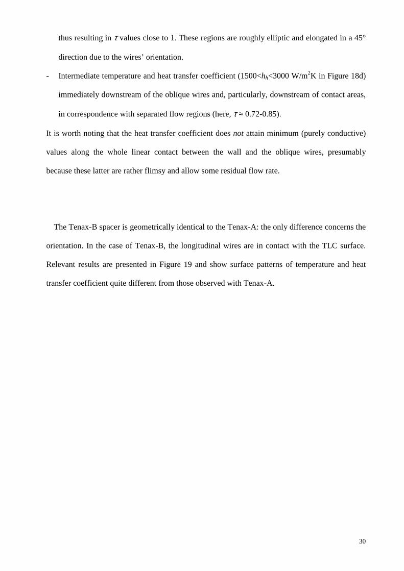
Relevant results are presented in Figure 19 and show surface patterns of temperature and heat
transfer coefficient quite different from those observed with Tenax-A.
31
Figure 19. Images obtained with the Tenax-B spacer at Qh=163 l/h, Th=34.75°C, Qc=1100 l/h, Tc=14.6°C: a) Typical test region showing the TLC surface along with an arrow indicating the main flow direction; b) Distribution of local temperature [°C] on the TLC surface; c) Distribution of the local hot-side heat transfer coefficient [W/m2K] along with lines showing the location of the spacer wires.
As also already observed in Figure 18 for the Tenax-A spacer, the lowest values of hh (purely
conductive heat transfer) occur in the zones where the two arrays of spacer wires intersect, due to
the tight contact between the wall and the near-wall wires (which in this case are the thick,
longitudinal ones). The highest hh can be observed in the central strips between the longitudinal
wires, without a clear relation with the location of the thinner oblique wires. Smaller, crescent-
shaped, regions of high heat transfer occur also upstream of the contact spots and downstream of
the thick wires. The maximum τ exhibited by the Tenax-B configuration is equal to ~0.89 which
is lower than that found for the Tenax-A configuration.
32
It is worth noting how the irregular shape of filaments generates also an irregular distribution
of temperatures and heat transfer coefficients, leading, for example, to a TLC-spacer contact area
corresponding to the crossing of the longitudinal and oblique filaments.
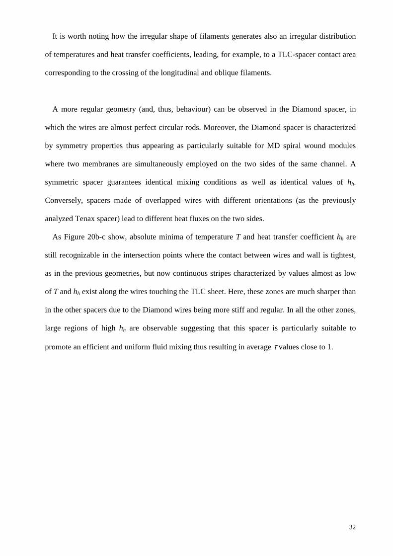
A more regular geometry (and, thus, behaviour) can be observed in the Diamond spacer, in
which the wires are almost perfect circular rods. Moreover, the Diamond spacer is characterized
by symmetry properties thus appearing as particularly suitable for MD spiral wound modules
where two membranes are simultaneously employed on the two sides of the same channel. A
symmetric spacer guarantees identical mixing conditions as well as identical values of hh.
Conversely, spacers made of overlapped wires with different orientations (as the previously
analyzed Tenax spacer) lead to different heat fluxes on the two sides.
As Figure 20b-c show, absolute minima of temperature T and heat transfer coefficient hh are
still recognizable in the intersection points where the contact between wires and wall is tightest,
as in the previous geometries, but now continuous stripes characterized by values almost as low
of T and hh exist along the wires touching the TLC sheet. Here, these zones are much sharper than
in the other spacers due to the Diamond wires being more stiff and regular. In all the other zones,
large regions of high hh are observable suggesting that this spacer is particularly suitable to
promote an efficient and uniform fluid mixing thus resulting in average τ values close to 1.
33
Figure 20. Images obtained with the Diamond spacer at Qh=163 l/h, Th=35.65°C,Qc=1000 l/h, Tc=14.55°C: a) Typical test region showing the TLC surface along with an arrow indicating the main flow direction; b) Distribution of local temperature [°C] on the TLC surface; c) Distribution of the local hot-side heat transfer coefficient [W/m2K] along with lines showing the location of the spacer wires.
4.2 Comparison between spacers
By letting the flow rate in the hot channel vary from 60 l/h to 160 l/h and post-processing images
and data for each spacer, a comparison was conducted between different spacer geometries.
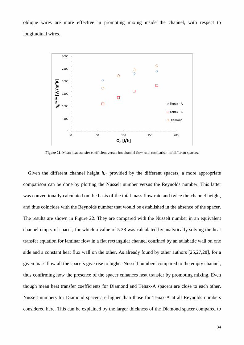
Figure 21 shows how the mean heat transfer coefficient varies with the hot water flow rate Qh for
the tested spacers. Tenax-A and Diamond, both with oblique wires close to the conductive wall,
present higher hh in the whole Qh range investigated with respect to Tenax-B, thus indicating that
34
oblique wires are more effective in promoting mixing inside the channel, with respect to
longitudinal wires.
0
500
1000
1500
2000
2500
3000
0 50 100 150 200
hh
me
an
[W/m
2K
]
Qh [l/h]
Tenax - A
Tenax - B
Diamond
Figure 21. Mean heat transfer coefficient versus hot channel flow rate: comparison of different spacers.
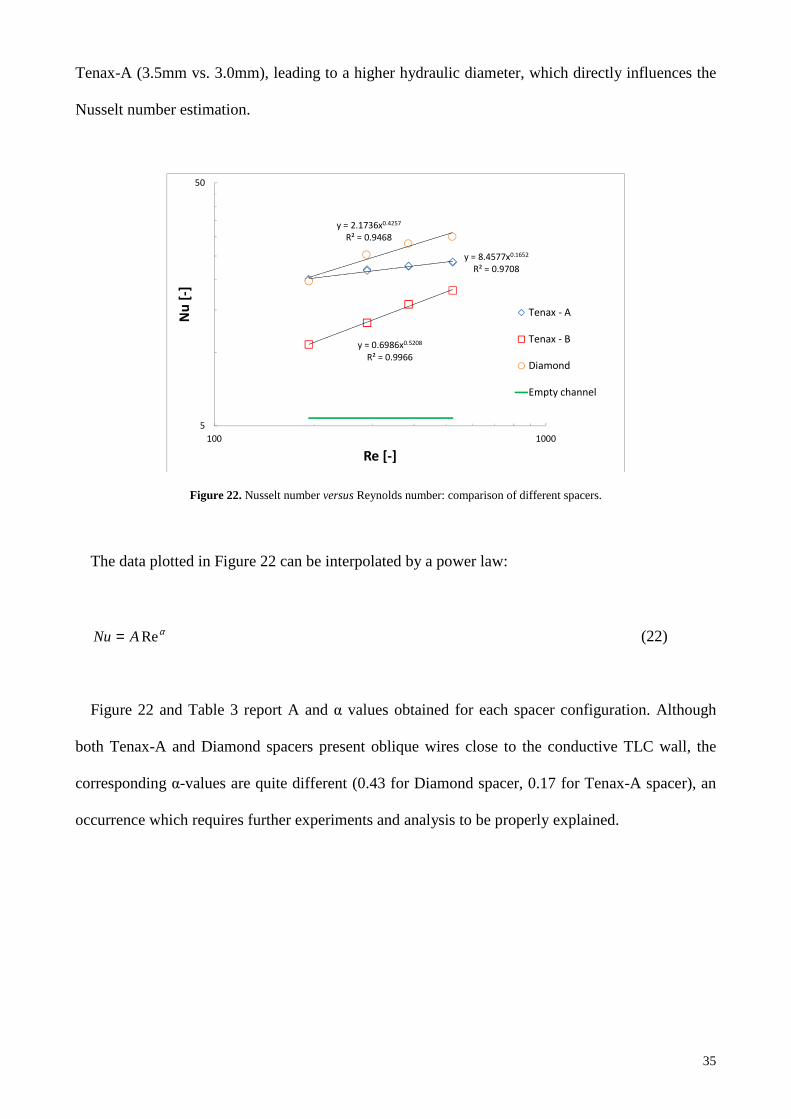
Given the different channel height hch provided by the different spacers, a more appropriate
comparison can be done by plotting the Nusselt number versus the Reynolds number. This latter
was conventionally calculated on the basis of the total mass flow rate and twice the channel height,
and thus coincides with the Reynolds number that would be established in the absence of the spacer.
The results are shown in Figure 22. They are compared with the Nusselt number in an equivalent
channel empty of spacer, for which a value of 5.38 was calculated by analytically solving the heat
transfer equation for laminar flow in a flat rectangular channel confined by an adiabatic wall on one
side and a constant heat flux wall on the other. As already found by other authors [25,27,28], for a
given mass flow all the spacers give rise to higher Nusselt numbers compared to the empty channel,
thus confirming how the presence of the spacer enhances heat transfer by promoting mixing. Even
though mean heat transfer coefficients for Diamond and Tenax-A spacers are close to each other,
Nusselt numbers for Diamond spacer are higher than those for Tenax-A at all Reynolds numbers
considered here. This can be explained by the larger thickness of the Diamond spacer compared to
35
Tenax-A (3.5mm vs. 3.0mm), leading to a higher hydraulic diameter, which directly influences the
Nusselt number estimation.
y = 8.4577x0.1652
R² = 0.9708
y = 0.6986x0.5208
R² = 0.9966
y = 2.1736x0.4257
R² = 0.9468
5
50
100 1000
Nu
[-]
Re [-]
Tenax - A
Tenax - B
Diamond
Empty channel
Figure 22. Nusselt number versus Reynolds number: comparison of different spacers.
The data plotted in Figure 22 can be interpolated by a power law:
αReANu = (22)
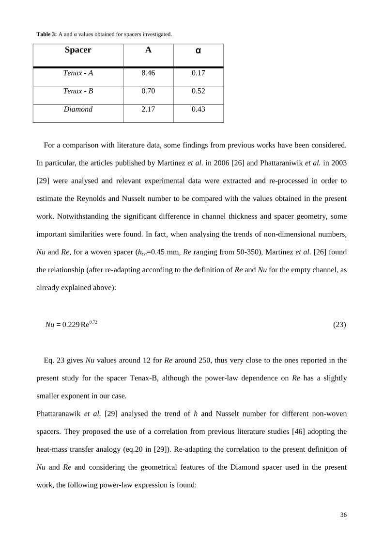
Figure 22 and Table 3 report A and α values obtained for each spacer configuration. Although
both Tenax-A and Diamond spacers present oblique wires close to the conductive TLC wall, the
corresponding α-values are quite different (0.43 for Diamond spacer, 0.17 for Tenax-A spacer), an
occurrence which requires further experiments and analysis to be properly explained.
36
Table 3: A and α values obtained for spacers investigated.
Spacer A αααα
Tenax - A 8.46 0.17
Tenax - B 0.70 0.52
Diamond 2.17 0.43
For a comparison with literature data, some findings from previous works have been considered.
In particular, the articles published by Martinez et al. in 2006 [26] and Phattaraniwik et al. in 2003
[29] were analysed and relevant experimental data were extracted and re-processed in order to
estimate the Reynolds and Nusselt number to be compared with the values obtained in the present
work. Notwithstanding the significant difference in channel thickness and spacer geometry, some
important similarities were found. In fact, when analysing the trends of non-dimensional numbers,
Nu and Re, for a woven spacer (hch=0.45 mm, Re ranging from 50-350), Martinez et al. [26] found
the relationship (after re-adapting according to the definition of Re and Nu for the empty channel, as
already explained above):
72.0Re229.0=Nu (23)
Eq. 23 gives Nu values around 12 for Re around 250, thus very close to the ones reported in the
present study for the spacer Tenax-B, although the power-law dependence on Re has a slightly
smaller exponent in our case.
Phattaranawik et al. [29] analysed the trend of h and Nusselt number for different non-woven
spacers. They proposed the use of a correlation from previous literature studies [46] adopting the
heat-mass transfer analogy (eq.20 in [29]). Re-adapting the correlation to the present definition of
Nu and Re and considering the geometrical features of the Diamond spacer used in the present
work, the following power-law expression is found:
37
5.0Re13.2=Nu (24)
Starting from this equation, calculations show that for Re around 250 a Nu value around 34 is
found, compared to a smaller value of about 23 obtained for the Diamond spacer in the present
investigation. At the same time, a similar exponent of the power law relating Nu vs Re can be
observed in the two cases.
Although being only qualitative comparisons, given the different geometries and experimental
approaches adopted in previous literature works, the fair agreement found between the TLC-IA-TP
technique and such previous findings encourage towards a further use of the hereby presented
experimental technique for wider investigations of the behaviour of spacer filled channels for
membrane distillation.
5 CONCLUSIONS
A space-resolved thermographic technique based on thermochromic liquid crystals (TLCs) was
developed in order to estimate the temperature and heat transfer coefficient distributions in spacer-
filled channels for Membrane Distillation modules. A purposely designed experimental apparatus
was set-up and used for testing different spacer configurations. Raw images were recorded and
post-processed using the Matlab® Image Processing Toolbox. The technique proved to be able to
provide local distributions of temperature on the membrane surface, heat transfer and thermal
polarization coefficients, allowing these quantities to be correlated with the geometrical features of
each spacer. Preliminary results show that:
- Oblique wires generate velocity components perpendicular to the conductive wall, which
improve convective heat transfer in the channel;
- Minimum heat transfer coefficients occur where spacers are in direct contact with the wall;
- Low heat transfer coefficients are observed downstream of these direct contact areas;
- For all the spacers considered here, a significant enhancement of the average Nusselt number
(from 2.5 up to 5.8 times that in an empty channel) is observed. Among them, the symmetric
38
and wide meshed Diamond spacer seems better to promote mixing conditions and heat
transfer;
- In the range investigated, the Nusselt number was found to increase with Re following a weak
power law, with exponents ranging from 0.17 to 0.52 according to the spatial configuration
tested.
The technique has proved to be quite promising and further investigations will be performed in
order to fully characterize mixing and heat transfer phenomena promotion in spacer-filled channels
for Membrane Distillation modules.
ACKNOWLEDGEMENTS
This work was carried out with the financial support of the MEDIRAS project within the EU-FP7
research programme (contract number TREN/FP7EN/218938). Tenax SpA, Solar Spring GmbH
and NSW (poly-net®) are gratefully acknowledged for providing the spacer material for the tests.
NOMENCLATURE
Symbol Quantity SI Unit A Pre-exponential factor - dh Hydraulic diameter m dh0 Void hydraulic diameter (≈2·hch) m dw Wire diameter m h Heat transfer coefficient W/(m2K) hch Channel height (= spacer thickness) m L Height/Length m lm Spacer wire pitch m N Molar flux mol/(m2s) Nu Nusselt number, (h·dh0/λ) - Pr Prandtl number - q Heat flux W/m2 Q Flow rate m3/s Re Reynolds number, (ρ·ū·dh0/µ) - T Temperature °K ū Mean velocity in the channel m/s x Main flow direction (longitudinal) m y Orthogonal direction m α Exponential factor - ε Voidage (porosity) - λ Thermal conductivity W(mK) µ Viscosity Pa·s
39
ρ Density Kg/m3 θ Reduced temperature °C σ Uncertainty variable τ Temperature Polarization coefficient - ζ Angle between crossing wires ° Subscripts
c Cold h Hot pol Polycarbonate TLC Thermochromic Liquid Crystals
REFERENCES
[1] K.W. Lawson, D.R. Lloyd, Membrane distillation, J. Membr. Sci. 124 (1997) 1–25.
[2] M.S. El-Bourawi, Z. Ding, R. Ma, M. Khayet, A framework for better understanding membrane distillation separation process, J. Membr. Sci. 285 (2006) 4–29.
[3] A. Cipollina, J. Koschikowski, F. Gross, D. Pfeifle, M. Rolletschek, R. Schwantes, Membrane distillation: solar and waste heat driven demonstration plants for desalination, International Workshop on Membrane Distillation and Related Technologies, October 9-12 (2011) Ravello (Italy)
[4] J. Koschikowski, M. Wieghaus, M. Rommel, V.S. Ortin, B.P. Suarez, J.R. Betancort Rodríguez, J.R., Experimental investigations on solar driven stand-alone membrane distillation systems for remote areas, Desalination 248 (1-3) (2009) 125-131.
[5] R. Porrazzo, A. Cipollina, M. Galluzzo, G. Micale, A neural network-based optimizing control system for a seawater-desalination solar-powered membrane distillation unit, Computers & Chemical Engineering, 54 (2013) 79– 96. Doi. 10.1016/j.compchemeng.2013.03.015
[6] J. Koschikowski, M.Wieghaus, M. Rommel, Solar thermal-driven desalination plants based on membrane distillation, Desalination 156 (2003) 295–304.
[7] Schwantes R., Cipollina A., Gross F., Koschikowski J., Pfeifle D., Rolletschek M., Subiela V., Membrane Distillation: solar and waste heat driven demonstration plants for desalination, Desalination (2013). Doi:10.1016/j.desal.2013.04.011
[8] R.W. Schofield, A.G. Fane, C.J.D. Fell, Heat and mass transfer in membrane distillation, J. Mem. Sci. 33 (3) (1987) 299-313.
[9] A. Cipollina, M. G. Di Sparti, A. Tamburini, G. Micale. Development of a Membrane Distillation module for solar energy seawater desalination, Chem. Eng. Res. Des. 90 (2012) 2101-2121.
[10] D. Winter, J. Koschikowski, M. Wieghaus, Desalination using membrane distillation: Experimental studies on full scale spiral wound modules, J. of Mem. Sci. 375 (1-2) (2011) 104-112.
[11] L. Martínez-Díez, M.I. Vázquez-González, F.J. Florido-Díaz, Study of membrane distillation using channel spacers, Journal of Membrane Science 144 (1-2) (1998) 45-56.
[12] C.P. Koutsou, S.G. Yiantsios, A.J. Karabelas, Direct numerical simulation of flow in spacer-filled channels: Effect of spacer geometrical characteristics, Journal of Membrane Science 291 (1-2) (2007) 53-69.
40
[13]Y.-L. Li, K.-L. Tung, CFD simulation of fluid flow through spacer-filled membrane module: Selecting suitable cell types for periodic boundary conditions, Desalination 233 (2008) 351–358.
[14] A. Tamburini, G. La Barbera, A. Cipollina, M. Ciofalo, G. Micale, CFD simulation of channels for direct and reverse electrodialysis, Desalination and Water Treatment, 48 (2012) 370–389.
[15] L. Gurreri, A. Tamburini, A. Cipollina, G. Micale, CFD analysis of the fluid flow behaviour in a reverse electrodialysis stack, Desalination and Water Treatment, 48 (2012) 390–403.
[16]L. Gurreri, A. Tamburini, A. Cipollina, G. Micale, M. Ciofalo, CFD Simulation of Mass Transfer Phenomena in Spacer Filled Channels for Reverse Electrodialysis Applications, Chemical Engineering Transactions 32 (2013) 1879-1884. Doi: 10.3303/CET1332314.
[17]J. Phattaranawik, R. Jiraratananon, A. G. Fane. Effects of net-type spacers on heat and mass transfer in direct contact membrane distillation and comparison with ultrafiltration studies, Journal of Membrane Science 217 (2003a) 193–206.
[18]L. Martìnez, J.M. Rodrìguez-Maroto, Effects of membrane and module design improvements on flux in direct contact membrane distillation, Desalination 205 (1-3) (2007) 97-103
[19]X. Yang, R. Wang, A.G. Fane, Novel designs for improving the performance of hollow fiber membrane distillation modules, Journal of Membrane Science 384 (1-2) (2011) 52-62.
[20] A. Cipollina, G. Micale, L. Rizzuti, Membrane distillation heat transfer enhancement by CFD analysis of internal module geometry, Desalination and Water Treatment 25 (2011) 195-209.
[21] A. Cipollina, A. Di Miceli, J. Koschikowski, G. Micale, L. Rizzuti, CFD simulation of a membrane distillation module channel, Desalination and Water Treatment 6 (2009) 177-183.
[22] A. R. Da Costa, A. G. Fane. Net-type spacers: effect of configuration on fluid flow path and ultrafiltration flux. Ind. Eng. Chem. Res. 33 (1994) 1845-1851.
[23]M. Shakaib, M. Ehtesham-ul Haq, I. Ahmad, R.M. Yunus, Modeling the effect of spacer orientation on heat transfer in membrane distillation, World Academy of Science, Engineering and Technology 72 (2010) 279-282.
[24]M. Shakaib, S.M.F. Hasani, I. Ahmed, R.M. Yunus, A CFD study on the effect of spacer orientation on temperature polarization in membrane distillation modules, Desalination 284 (2012) 332-340.
[25] J. Phattaranawik, R. Jiraratananon, A.G. Fane, C. Halim, Mass flux enhancement using filled channels in direct contact membrane distillation, Journal of Membrane Science (2001) 193-201.
[26] L. Martìnez, J.M. Rodrìguez-Maroto, Characterization of membrane distillation modules and analysis of mass flux enhancement by channel spacers, Journal of Membrane Science 274 (2006) 123–137.
[27] M.N. Chernyshov, G.W. Meindersma, A.B. de Haan, Comparison of spacers for temperature polarization reduction in air gap membrane distillation, Desalination 183 (2005) 363-374.
[28] Y. Yun, J. Wang, R. Ma, A.G. Fane, Effects of channel spacers on direct contact membrane distillation, Des. & Water Treatment 34 (2011) 63-69.
[29]J. Phattaranawik, R. Jiraratananon, A. G. Fane, Heat transport and membrane distillation coefficients in direct contact membrane distillation, Journal of Membrane Science 212 (2003b) 177–193.
[30]X. Yang, H. Yu, R. Wang, A.G. Fane, Analysis of the effect of turbulence promoters in hollow fiber membrane distillation modules by computational fluid dynamic (CFD) simulations, Journal of Membrane Science 415-416 (2012) 758-769.
41
[31]S. Al-Sharif, M. Albeirutty, A. Cipollina, G. Micale, Modelling flow and heat transfer in spacer-filled membrane distillation channels using open source CFD code, Desalination 311 (2013) 103-112.
[32]C.-C. Wang, On the heat transfer correlation for membrane distillation, Energy Conversion and Management 52 (4) (2011) 1968-1973.
[33] A. Tamburini, A. Parlapiano, A. Cipollina, M. Ciofalo, G. Micale, Temperature Distribution Analysis in Spacer Filled Channels for Membrane Distillation, Procs. 7th International Symposium on Turbulence, Heat and Mass Transfer, Palermo, Italy, 24-27 September 2012, pp. 299-302, K. Hanjalic, Y. Nagano, D. Borello and D. Jakirlic, eds, Begell House Inc., New York, 2012.
[34]A. Tamburini, G. Micale, M. Ciofalo, A. Cipollina, Experimental Analysis via Thermochromic Liquid Crystals of the temperature local distribution in Membrane Distillation modules, Chemical Engineering Transactions 32 (2013) 2041-2046. Doi: 10.3303/CET1332341.
[35]L.C.R Hallcrest, Hallcrest Handbook of Thermochromic Liquid Crystal Technology, http://hallcrest.com/randt.cfm (1991).
[36]V.U. Kakade, G.D. Lock, M. Wilson, J.M. Owen, J.E. Mayhew, Accurate heat transfer measurements using thermochromic liquid crystal. Part 2: Application to a rotating disc, International Journal of Heat and Fluid Flow 30 (2009) 950–959.
[37]P. J. Newton, Y. Yan, Nia E. Stevens, S. T. Evatt, Gary D. Lock, J. Michael Owen, Transient heat transfer measurements using thermochromic liquid crystal. Part 1: An improved technique, International Journal of Heat and Fluid Flow 24 (2003) 14–22.
[38]M. Ciofalo, I. Di Piazza, J. A. Stasiek, Investigation of Flow and Heat Transfer in Corrugated-Undulated Plate Heat Exchangers, Heat and Mass Transfer, 36 (2000) 449-462.
[39]J. Stasiek, M. Ciofalo, M. Wierzbowski, Experimental and numerical simulations of flow and heat transfer in heat exchanger elements using liquid crystal thermography, Journal of Thermal Science 13 (2) (2004) 133-137.
[40]J.A. Stasiek, T.A. Kowalewski, Thermochromic Liquid Crystals applied for heat transfer research, Opto-electronics Review 10(1) (2002) 1-10.
[41]W.J. Hiller, S. Koch, T.A. Kowalewski, Three-dimensional structures in laminar natural convection in a cubic enclosure, Exp. Thermal and Fluid Sci., 2(1) (1989) 34-44.
[42]M. Ciofalo, M. Signorino, M. Simiano, Tomographic particle-image velocimetry and thermography in Rayleigh-Bénard convection using suspended thermochromic liquid crystals and digital image processing, Experiments in Fluids 34 (2003) 156-172.
[43]H. Al-Fulaij, A. Cipollina, D. Bogle, and H. Ettouney, Once through multistage flash desalination: gPROMS dynamic and steady state modelling, Desalination and Water Treatment 18 (2010) 46-60.
[44] M. Tedesco, A. Cipollina, A. Tamburini, W. van Baak, G. Micale, Modelling the Reverse ElectroDialysis process with seawater and concentrated brines, Desalination and Water Treatment 49 (2012) 404-424.
[45]R.J. Moffat, Describing the uncertainties in experimental results, Experimental Thermal and Fluid Science 1 (1988) 3-17.
[46]A.R. Da Costa, A.G. Fane, D.E. Wiley, Spacer characterization and pressure drop modeling in spacer-filled channels for ultrafiltration, J. Membr. Sci. 87 (1994) 79–98.