arX

iv:p

hysi

cs/0

4060

96v1

[ph

ysic

s.fl

u-dy

n] 2

2 Ju

n 20

04

Gravity waves over topographical bottoms: Comparison with the

experiment

Meng-Jie Huang, Chao-Hsien Kuo, and Zhen Ye∗

Wave Phenomena Lab, Department of Physics,

National Central University, Chungli, Taiwan

Abstract

In this paper, the propagation of water surface waves over one-dimensional periodic and random

bottoms is investigated by the transfer matrix method. For the periodic bottoms, the band struc-

ture is calculated, and the results are compared to the transmission results. When the bottoms

are randomized, the Anderson localization phenomenon is observed. The theory has been applied

to an existing experiment (Belzons, et al., J. Fluid Mech. 186, 530 (1988)). In general, the results

are compared favorably with the experimental observation.

PACS numbers: 47.10.+g, 47.11.+j, 47.35.+i.

∗Electronic address: zhen@shaw.ca

1

I. INTRODUCTION

Multiple scattering occurs when waves propagate in media with scatterers, leading to

many interesting phenomena such as the bandgaps in periodically structured media and

the Anderson localization in disordered media[1]. Within a bandgap, waves are evanescent;

when localized, they remain confined spatially near the transmission point until dissipated.

The phenomenon of bandgaps and localization has been both extensively and intensively

studied for electronic, electromagnetic, and acoustic systems, as summarized in Ref. [2].

Propagation and scattering of gravity waves over topographical bottoms has also been

and continues to be a subject of much research. From practical perspectives, it is essential

to many important ocean engineering problems such as designing underwater structures in

minimizing the impact of water waves on banks. From the point of fundamental research, the

system of water waves may also play an important role. Since water waves are a macroscopic

phenomenon, they may be monitored and recorded in a laboratory scale. In this way, many

significant phenomena of microscopic scales may be demonstrated with water waves. This

would be particularly useful in facilitating the understanding of abstract concepts which

may have been initiated for quantum waves. A great amount of papers and monographs

has been published on water waves over various topographical bottoms [3, 4, 5, 6, 7, 8, 9,

10, 11, 12, 13, 14]. A comprehensive reference on the topic can be found in three excellent

textbooks [15, 16, 17].

The concept of bandgaps and Anderson localization has been extended to the the study

of the propagation of water surface waves over topographical bottoms. In 1983, Guazzelli

et al. [18] suggested that the phenomenon of Anderson localization could be observed

on shallow water waves, when the bottom has random structures. Later, Devillard et al.

reconsidered water wave localization inside a channel with a random bottom in a framework

of the potential theory [19]. They computed the localization length for various cases. The

experimental observation of water wave localization has been subsequently suggested by

Belzone et al.[20].

When the topographical bottoms are periodically structured, the propagation of water

surface waves will be modulated accordingly. According to Bloch theorem, waves in a

periodic medium, now termed as Bloch waves, can be expressed in terms of the product of a

plane wave and a periodic function which is has the periodicity of the medium. Therefore, the

2

waves will exhibit the properties of both plane wave propagation and periodic modulation.

Indeed, a recent experiment[21] has used gravity waves to illustrate the phenomenon of

Bloch wave over a two dimensional periodic bottom. This pioneering experiment has made

it possible that the abstract concept be presented in an unprecedentedly clear manner. The

experimental results have also been matched by a theoretical analysis in Ref. [22].

The experimental advantures[20, 21] pave a new avenue for investigating the phenomena

of Anderson localization in disordered media and wave bandgaps in periodic structures. In

particular, it has been recognized that the two dimension is a marginal dimension, many

peculiar wave phenomena could be expected[24]. Since gravity waves are naturally a two

dimensional phenomenon, it may be expected that water surface waves can play a role in

demonstrating some of the peculiar wave phenomena.

Motivated by the developments, we wish to further consider the propagation and localiza-

tion properties of water surface waves. At the first stage, we will consider water waves over

one dimensional uneven bottoms. We present a theoretical analysis of the previous experi-

mental results[20]. The formulation in Ref. [23] will be used for the purpose. The comparison

between the experimental and theoretical results, in return, provides a verification of the

theory. We will study the band structure of periodic cases, the effect of randomness on wave

propagation, the relation between the bandgaps and the localization, and the amplitude or

energy distribution over the structured bottoms. The dependence on parameters, such as

the frequency, water depth, the variations of the height and width of the obstacle steps, will

be examined in detail. Although the experiment to be analyzed here was done nearly twenty

years ago, to the best of our knowledge, however, there are no further experiments which

have been done on water waves in the context of the localization effects. Even the existing

limited experimental results have not been thoroughly analyzed. The present paper is to

bridge the gaps, with the hope that further experimental investigation may be arranged.

The paper will be constructed as follows. In the next section, we will present the formu-

lation and parametrization for the problem. The results and discussion will be presented in

section III, followed by a summary in section IV.

3

II. THE GENERAL FORMULATION

A theory of water wave propagation over step-mounted bottoms has been recently pro-

posed and developed in Refs. [22, 23]. This formulation has been used earlier in interpreting

some experimental data [22]. While the details can be referred to in Ref. [23], here we only

present the final equation. After the Fourier transformation, the equation describing the

wave of frequency ω over topographical bottoms is

∇(

1

k2∇η

)

+ η = 0, (1)

where k satisfies

ω2 = gk(~r) tanh(k(~r)h(~r)), (2)

where η is the surface displacement, g is the gravity acceleration constant, and h is the

depth from the surface. For a fixed frequency, the variation of the wavenumber k with the

topographical bottom is determined by the depth function h.

From Eq. (1), we have the conditions linking domains with different depths as follows:

both η and tanh(kh)k

η = ω2

gk2η are continuous across the boundary.

A. Application to one-dimensional situations

1. A single step

First, consider a step with width d, and a wave is propagating along the x direction. The

conceptual layout is in Fig. 1(a). We use the standard transfer matrix method to solve for

the wave transmission across the step.

The waves on the left, within, and on the right side of the step can be generally rewritten

as

ηL = ALeikLx +BLe

−ikLx

ηM = AMeikMx +BMe−ikMx

ηR = AReikRx +BRe

−ikRx. (3)

The subscripts L,M,R represent the quantities on the left side, in the middle, and on the

right side of the step respectively.

The boundary conditions lead to the following equations:

4

ALeikLxL +BLe

−ikLxL = AMeikMxL + BMe−ikMxL; (4)

1

kL

(

ALeikLxL −BMe−ikLxL

)

=1

kM

(

AMeikMxL − BMe−ikMxL

)

, (5)

and

AMeikMxR +BMe−ikMxR = AReikRxR +BRe

−ikRxR; (6)

1

kM

(

AMeikMxR − BMe−ikMxR

)

=1

kR

(

AReikRxR −BRe

−ikRxR

)

. (7)

In these equations, xL,R stands for the locations of the left and right sides of the step

respectively, and xR − xL = d.

The first set of boundary equations gives the matrix relation

AL

BL

= TLM

AM

BM

(8)

with

TLM =1

2

(1 + gLM)ei(kM−kL)xL (1− gLM)e−i(kM+kL)xL

(1− gLM)ei(kM+kL)xL (1 + gLM)e−i(kM−kL)xL

, (9)

and

gLM =kLkM

.

Similarly, we can derive

AM

BM

= TMR

AR

BR

(10)

with

TMR =1

2

(1 + gMR)ei(kR−kM )xR (1− gMR)e

−i(kR+kM )xR

(1− gMR)ei(kR+kM )xR (1 + gMR)e

−i(kR−kM )xR

(11)

and

gMR =kMkR

.

From Eqs. (9) and (11), we obtain the following solution in the transfer matrix form

AL

BL

= TLR

AR

BR

(12)

5

with

TLR = TLMTMR. (13)

Eq. (12) relates the waves on the left to the right side of the step.

2. The case of N steps

Now we consider N steps in a unform medium of wave number k. The illustration is in

Fig. 1(b). The step widths are di and the water depths over the steps are hi. The wave

number over the step is denoted by ki (i = 1, . . . , N). They satisfy the following relations

respectively,

ω2 = gh tanh(kh), ω2 = ghi tanh(kihi). (14)

Clearly, the coefficients on the most left hand region is related to the most right hand

region by

AL

BL

= T (N)

AR

BR

(15)

with

T (N) =N∏

i=1

Ti (16)

The matrix Ti is the transfer matrix for the i-th step and will be given below.

Let us consider a unit plane wave propagation along the x direction, and explore the

reflection and transmission properties. In this case, clearly we have

AL = 1, BR = 0. (17)

BR = 0 is the common radiation condition. Thus from Eq. (15) we arrive at the solutions

AR(N) =1

T11(N), BL(N) =

T21(N)

T11(N). (18)

The subscripts denote the corresponding matrix elements.

The transmission and reflection coefficients are defined as

T = |AR(N)|2, R = 1− T. (19)

Now we construct the T matrix for each step. In the current case, we have

gLM(i) =k

ki, gMR(i) =

kik, (20)

6

and

kL = k, kM = ki, kR = k. (21)

We denote gs,i =kki. Therefore

Ti =1

4

(1 + gs,i)ei(ki−k)xi,L (1− gs,i)e

−i(ki+k)xi,L

(1− gs,i)ei(k+ki)xi,L (1 + gs,i)e

−i(ki−k)xi,L

×

(1 + 1/gs,i)ei(k−ki)xi,R (1− 1/gs,i)e

−i(k+ki)xi,R

(1− 1/gs,i)ei(k+ki)xi,R (1 + 1/gs,i)e

−i(k−ki)xi,R

(22)

B. Simulation setup

1. Non-dimensional parametrization

Consider an infinite periodic array of the steps, as shown in Fig. 1. The lattice constant

is L. For random arrays, L refers to the average distance between two adjacent steps.

The dispersion relation is

ω2 = gk tanh(kh).

This can be rewritten asω2

ω20

= (kL) tanh

(

(kL)h

L

)

,

with

ω20 =

g

L.

Therefore in all later computations, the length can be scaled by L, the frequency by ω0, the

wavenumber by kL.

The wavenumbers in the medium and within the steps are given by (at the same fre-

quency)

ω2

ω20

= (kL) tanh

(

(kL)h

L

)

, (23)

ω2

ω20

= (kiL) tanh

(

(kiL)hi

L

)

. (24)

This leads to

gs,i =kL

kiL,

and the transfer matrix of the i-th step is

7

T (i) =1

4

(1 + gs,i)ei(kiL−kL)

xi,L

L (1− gs,i)e−i(kiL+kL)

xi,L

L

(1− gs,i)ei(kL+kiL)

xi,L

L (1 + gs,i)e−i(kiL−kL)

xi,L

L

×

(1 + 1gs,i

)ei(kL−kiL)xi,L+di

L (1− 1gs,i

)e−i(kL+kiL)xi,L+di

L

(1− 1gs,i

)ei(kL+kiL)x1,L+di

L (1 + 1gs,i

)e−i(kL−kiL)xi,L+di

L

, (25)

where xi,L is the coordinate of the left side of the i-th step.

2. Band structure for periodic cases

For the periodically arranged steps with di = d, and hi = h1, the band structure can be

solved. According to Bloch theorem, the water surface displacement η can be expressed as

η(x) = ξ(x)eiKx, (26)

where K is the Bloch wavenumber, and ξ(x) is a periodic function modulated by the peri-

odicity of the structure, i. e. ξ(x+ L) = ξ(x). The relation between K and the frequency ω

can be obtained by taking Eq. (26) into Eq. (15).

We can derive an equation determining the band structure in the periodic case,

cos(KL) = cos(k1L(d/L) cos(kL(L− d)/L)− cosh(2ξ) sin(k1L(d/L)) sin(kL(L− d)/L),

(27)

where

ξ = ln(q), with ω2 = gk1 tanh(kh1), q2 =k1k.

3. Random situations

There are a number of ways to introduce the randomness. (1) Variation in the height

of the steps: With the fixed widths and positions of the steps, the height of the steps can

be varied in a controlled way. For example, the height of the steps can be varied randomly

between [H0 −∆H,H0 +∆H ]. (2) Positional disorders: Initially, the steps can be arranged

in a lattice form. Then allow each step to move randomly around its initial position. The

allowing range for movement can be controlled and denotes the level of randomness. The

8

extreme case is completely randomness. (3) Width randomness: We can also introduce the

randomness for the widths of the steps. In the simulation, we will consider the randomness

introduced in the experiment[20].

When randomness is introduced, a few definitions are in order. The most important

quantity is the Lyapounov exponent γ. Its definition is

γ = limN→∞

〈γN〉, (28)

where

γN ≡ −1

Nln(|AR(N)|).

Here |AR(N)|2 is the transmission coefficient for a system with N random steps, referring

to Eq. (18),

|AR(N)|2 =1

|T11(N)|2.

The symbol 〈·〉 denotes the average over the random configuration. The inverse of the

Lyapounov exponent characterizes the localization length, i. e. ξ = γ−1N .

III. THE RESULTS AND DISCUSSION

The systems are from the previous experiment[20]. That is, the bottoms are mounted with

a series of steps and these steps are either regularly or randomly but on-average regularly

placed on the bottoms. Three cases are considered and are illustrated by Fig. 2. In the

Bed P case, the averaged water depth is H0, the periodicity is 2L0, and the step variation

is fixed at σH . In the Bed RS case, the averaged water depth is H0, the step variation is

fixed at σH , the separation between steps is uniformly distributed with [d0 −∆d, d0 +∆d].

In the Bed R case, both the height and the separation between the steps are allowed to vary

randomly, but within the ranges [H0 −∆H,H0 +∆H ] and [L0 −∆L, L0 +∆L] respectively.

The experimental setups have been described in Section 2 of Ref. [20]. We briefly repeat

here. The experiments were carried out in a glass-walled wave tank with length 4m and

width 0.39m. A bottom composed of periodic or random steps was built into a flat bottom

with the mean water depth H0. The different bottoms varied only along the tank so that,

apart from weak edge effects, the propagation of waves is considered to be one-dimensional.

The resolution of the water depth is estimated at about 0.2mm.

9

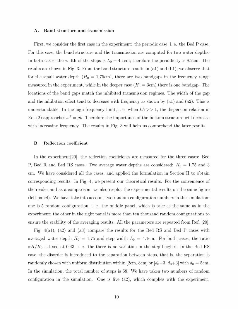
A. Band structure and transmission

First, we consider the first case in the experiment: the periodic case, i. e. the Bed P case.

For this case, the band structure and the transmission are computed for two water depths.

In both cases, the width of the steps is L0 = 4.1cm; therefore the periodicity is 8.2cm. The

results are shown in Fig. 3. From the band structure results in (a1) and (b1), we observe that

for the small water depth (H0 = 1.75cm), there are two bandgaps in the frequency range

measured in the experiment, while in the deeper case (H0 = 3cm) there is one bandgap. The

locations of the band gaps match the inhibited transmission regimes. The width of the gap

and the inhibition effect tend to decrease with frequency as shown by (a1) and (a2). This is

understandable. In the high frequency limit, i. e. when kh >> 1, the dispersion relation in

Eq. (2) approaches ω2 = gk. Therefore the importance of the bottom structure will decrease

with increasing frequency. The results in Fig. 3 will help us comprehend the later results.

B. Reflection coefficient

In the experiment[20], the reflection coefficients are measured for the three cases: Bed

P, Bed R and Bed RS cases. Two average water depths are considered: H0 = 1.75 and 3

cm. We have considered all the cases, and applied the formulation in Section II to obtain

corresponding results. In Fig. 4, we present our theoretical results. For the convenience of

the reader and as a comparison, we also re-plot the experimental results on the same figure

(left panel). We have take into account two random configuration numbers in the simulation:

one is 5 random configuration, i. e. the middle panel, which is take as the same as in the

experiment; the other in the right panel is more than ten thousand random configurations to

ensure the stability of the averaging results. All the parameters are repeated from Ref. [20].

Fig. 4(a1), (a2) and (a3) compare the results for the Bed RS and Bed P cases with

averaged water depth H0 = 1.75 and step width L0 = 4.1cm. For both cases, the ratio

σH/H0 is fixed at 0.43, i. e. the there is no variation in the step heights. In the Bed RS

case, the disorder is introduced to the separation between steps, that is, the separation is

randomly chosen with uniform distribution within [2cm, 8cm] or [d0−3, d0+3] with d0 = 5cm.

In the simulation, the total number of steps is 58. We have taken two numbers of random

configuration in the simulation. One is five (a2), which complies with the experiment,

10

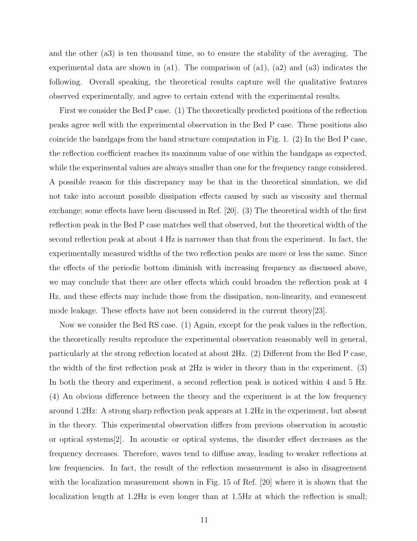
and the other (a3) is ten thousand time, so to ensure the stability of the averaging. The

experimental data are shown in (a1). The comparison of (a1), (a2) and (a3) indicates the

following. Overall speaking, the theoretical results capture well the qualitative features

observed experimentally, and agree to certain extend with the experimental results.

First we consider the Bed P case. (1) The theoretically predicted positions of the reflection

peaks agree well with the experimental observation in the Bed P case. These positions also

coincide the bandgaps from the band structure computation in Fig. 1. (2) In the Bed P case,

the reflection coefficient reaches its maximum value of one within the bandgaps as expected,

while the experimental values are always smaller than one for the frequency range considered.

A possible reason for this discrepancy may be that in the theoretical simulation, we did

not take into account possible dissipation effects caused by such as viscosity and thermal

exchange; some effects have been discussed in Ref. [20]. (3) The theoretical width of the first

reflection peak in the Bed P case matches well that observed, but the theoretical width of the

second reflection peak at about 4 Hz is narrower than that from the experiment. In fact, the

experimentally measured widths of the two reflection peaks are more or less the same. Since

the effects of the periodic bottom diminish with increasing frequency as discussed above,

we may conclude that there are other effects which could broaden the reflection peak at 4

Hz, and these effects may include those from the dissipation, non-linearity, and evanescent

mode leakage. These effects have not been considered in the current theory[23].

Now we consider the Bed RS case. (1) Again, except for the peak values in the reflection,

the theoretically results reproduce the experimental observation reasonably well in general,

particularly at the strong reflection located at about 2Hz. (2) Different from the Bed P case,

the width of the first reflection peak at 2Hz is wider in theory than in the experiment. (3)

In both the theory and experiment, a second reflection peak is noticed within 4 and 5 Hz.

(4) An obvious difference between the theory and the experiment is at the low frequency

around 1.2Hz: A strong sharp reflection peak appears at 1.2Hz in the experiment, but absent

in the theory. This experimental observation differs from previous observation in acoustic

or optical systems[2]. In acoustic or optical systems, the disorder effect decreases as the

frequency decreases. Therefore, waves tend to diffuse away, leading to weaker reflections at

low frequencies. In fact, the result of the reflection measurement is also in disagreement

with the localization measurement shown in Fig. 15 of Ref. [20] where it is shown that the

localization length at 1.2Hz is even longer than at 1.5Hz at which the reflection is small;

11

the longer the localization length, the weaker is the reflection. (5) Increasing the number of

random configuration tend to smooth the curves.

The comparison between the theoretical and experimental reflection results for the Bed

P and Bed R cases with H0 = 3cm is shown by Fig. 4(b1), (b2) and (b3). The parameters

are as follows. (1) Bed P: σH/H0 = 0.25, L0 = 4.1cm; (2) Bed R: the separation between

steps varies completely randomly within L0 ± ∆L with ∆L = 2cm, and the height of the

steps varies uniformly within H0 ±∆H with ∆H = 1.26cm. The number of steps is 58. In

(b2), five random configurations are used for averaging, and in (b3) ten thousand random

configurations are used to ensure the stability of the averaging. In the Bed P case, except at

the reflection peak, the theoretical results reproduce very well the experimental observation.

In the Bed R case, the theoretical results also match that from the experiment in both the

qualitative structure and the magnitude, referring to (b1) and (b2). The existing deviation

may result from the insufficient random average.

The comparison between the theoretical and experimental reflection results for the Bed

P and Bed R cases with H0 = 1.75cm is shown by Fig. 4(c1), (c2) and (c3). The parameters

are as follows. (1) Bed P: σH/H0 = 0.43, L0 = 4.1cm; (2) Bed R: the separation between

steps varies completely randomly within L0 ± ∆L with ∆L = 2cm, and the height of the

steps varies uniformly within H0 ±∆H with ∆H = 1.24cm. The number of steps is 58. In

(c2), five random configurations are used for averaging, and in (c3) ten thousand random

configurations are used to ensure the stability of the averaging. The Bed P case has been

discussed in the above. In the Bed R case, the general features of the experimental and

theoretical results seem to be agreeable with each other. The predicted reflection curve

starts to match qualitatively the experimental data from about 3 Hz. The discrepancy at

low frequencies is, again, noticeable.

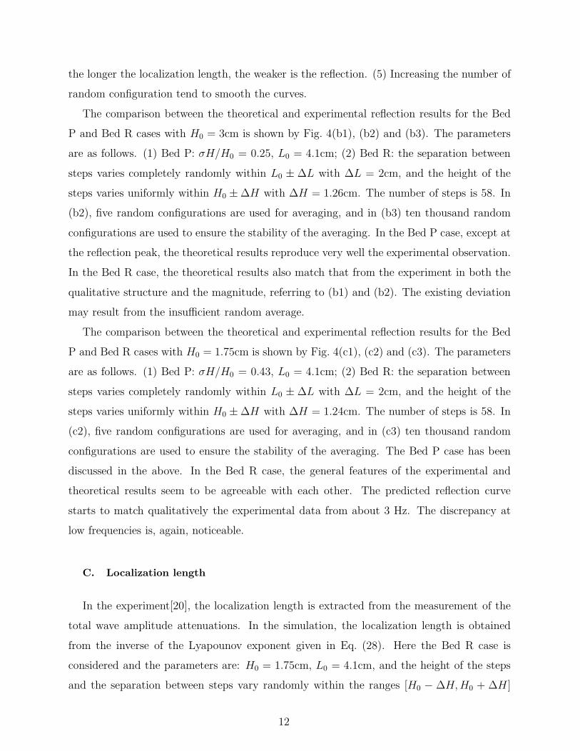
C. Localization length

In the experiment[20], the localization length is extracted from the measurement of the

total wave amplitude attenuations. In the simulation, the localization length is obtained

from the inverse of the Lyapounov exponent given in Eq. (28). Here the Bed R case is

considered and the parameters are: H0 = 1.75cm, L0 = 4.1cm, and the height of the steps

and the separation between steps vary randomly within the ranges [H0 − ∆H,H0 + ∆H ]

12

and [L0 −∆L, L0 +∆L] respectively; here ∆H = 1.2425cm, and ∆L = 2cm. Ten thousand

steps and ten thousand random configurations have been used in the simulation to ensure

the stability of the numerical results.

The numerical and experimental results are shown in Fig. 5. Here the localization length

is plotted against the frequency. The results from Ref. [20] are shown in the inserted box. A

few observations are in order. (1) In Ref. [20], the authors have used a potential formulation

to obtain the localization length, denoted by the solid length in the inserted box. By eye-

inspection, we see that the present numerical results agree remarkably well with the results

from the potential theory, thus providing another support for the present relatively simple

theory, stemmed from Ref. [23]. (2) The numerical results also agree with the averaged

experimental data in the vicinity of the frequency 2Hz. (3) There is a huge fluctuation in

the experiment results. From our simulation, we think that such a significant deviation

is due to the insufficient average numbers, an obvious limitation on any experiment. This

is particularly an important factor when the localization length is long. Nevertheless, the

agreements shown in Fig. 5 is encouraging.

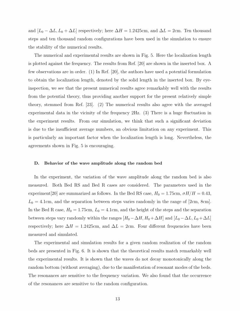
D. Behavior of the wave amplitude along the random bed

In the experiment, the variation of the wave amplitude along the random bed is also

measured. Both Bed RS and Bed R cases are considered. The parameters used in the

experiment[20] are summarized as follows. In the Bed RS case, H0 = 1.75cm, σH/H = 0.43,

L0 = 4.1cm, and the separation between steps varies randomly in the range of [2cm, 8cm].

In the Bed R case, H0 = 1.75cm, L0 = 4.1cm, and the height of the steps and the separation

between steps vary randomly within the ranges [H0−∆H,H0+∆H ] and [L0−∆L, L0+∆L]

respectively; here ∆H = 1.2425cm, and ∆L = 2cm. Four different frequencies have been

measured and simulated.

The experimental and simulation results for a given random realization of the random

beds are presented in Fig. 6. It is shown that the theoretical results match remarkably well

the experimental results. It is shown that the waves do not decay monotonically along the

random bottom (without averaging), due to the manifestation of resonant modes of the beds.

The resonances are sensitive to the frequency variation. We also found that the occurrence

of the resonances are sensitive to the random configuration.

13

We have further computed the averaged variation of the wave amplitude along the random

bed for a sufficiently large number of random configurations. We found that though smeared

out a little by the averaging, the resonance feature remains for spatial points near the

transmission and tends to diminish for large travelling paths. And the averaged amplitude

decays exponentially with increasing travelling distances. As an example, in Fig. 7 we

illustrate these by the results of the Bed RS case with f = 1.6Hz. The results in Fig. 7

also indicate that the exponential decay rate, associated with the localization length, may

not be accurately obtained from measurements done on insufficiently long samples, as the

fluctuation can be quite significant for small sample sizes.

IV. SUMMARY

In summary, we have considered the propagation of water surface waves over topograph-

ical bottoms. A transfer method has been developed to compute the wave field along the

propagating path, the transmission and reflection coefficients. The localization effects due

to disordered bottom structures are also considered. The theory has been applied to ana-

lyze the existing experimental results. Some agreements and discrepancies are discovered

and discussed. It is pointed out that more detailed experiments may be helpful in not only

identifying the peculiar localization phenomenon, but in helping improve theories for water

wave propagation over rough bottoms.

Acknowledgments

The work received support from the National Science Council (NSC-92-2611-M008-002).

[1] P. W. Anderson, Phys. Rev. 109, 1492 (1958).

[2] P. Sheng, Introduction to Wave Scattering, Localization, and Mesoscopic Phenomena (Aca-

demic Press, New York, 1995).

[3] M. S. Longuet-Higgins, J. Fluid Mech. 1, 163 (1956).

[4] E. F. Bartholomeuz, Proc. Cambridge Philos. Soc. 54, 106 (1958).

[5] J. W. Miles, J. Fluid Mech. 28, 755 (1967).

14

[6] D. H. Peregrine, Adv. Appl. Mech. 16, 9 (1979).

[7] R. E. Meyer, Adv. Appl. Mech. 19, 53 (1979).

[8] H. Kagemoto and D. K.-P. Yue, J. Fluid Mech. 166, 189 (1986).

[9] M. Belzons, E. Guazzelli, and O. Parodi, J. Fluid Mech. 186, 539 (1988).

[10] P. Devillard, F. Dunlop, and B. Souillard, J. Fluid Mech. 186, 521 (1988).

[11] C. M. Linton and D. V. Evans, J. Fluid Mech. 215, 549 (1990).

[12] J. N. Newman, J. Fluid Mech. 23, 399 (1965).

[13] A. Nachbin and G. C. Papanicolaou, J. Fluid Mech. 241, 311 (1992).

[14] J. H. Pihl, C.-C. Mei, and M. J. Hancock, Phys. Rev. E 66, 016611 (2002); G. L. Gratalop

and C.-C. Mei, Phys. Rev. E 68, 026314 (2003).

[15] H. Lamb, Hydrodynamics, (Dover, New York, 1932).

[16] C.-C. Mei, The Applied Dynamics of Ocean Surface Waves, (World Scientific, Singapore,

1989).

[17] M. W. Dingemans, Water Wave Propagation over Uneven Bottoms, (World Scientific, Singa-

pore, 1997).

[18] E. Guazzelli, E. Guyon, and B. Souillard, J. Phys. Lett. 44, L-837 (1983).

[19] P. Devillard, F. Dunlop, and B. Souillard, J. Fluid Mech. 186, 521 (1988).

[20] M. Belzones, E. Guazzelli, and O. Parodi, J. Fluid Mech. bf 186, 539 (1988).

[21] M. Torres, J. P. Adrados, F. R. Montero de Espinosa, Nature 398, 114 (1999).

[22] M. Torres, et al., Phys. Rev. E 63, 011204 (2000).

[23] Z. Ye, Phys. Rev. E 67, 036623 (2003).

[24] M. P. Marder, Condensed Matter Physics, (John Wiley & Sons, Inc., New York, 2000).

15

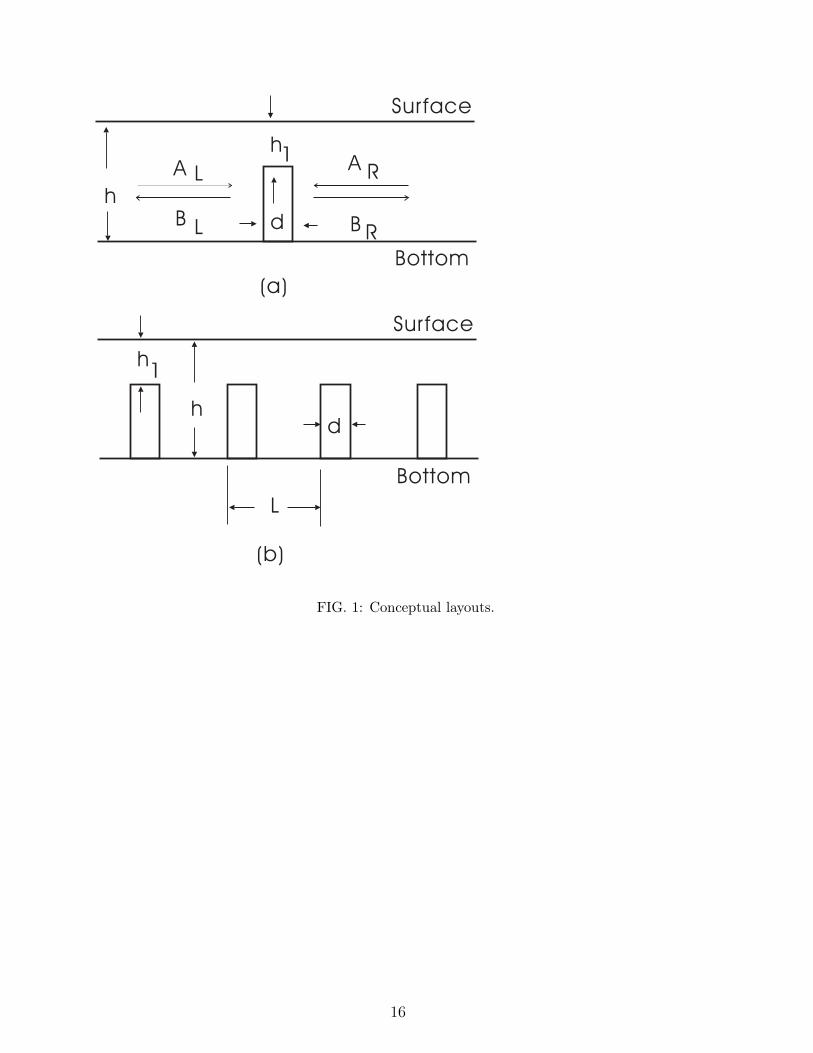
FIG. 1: Conceptual layouts.

16

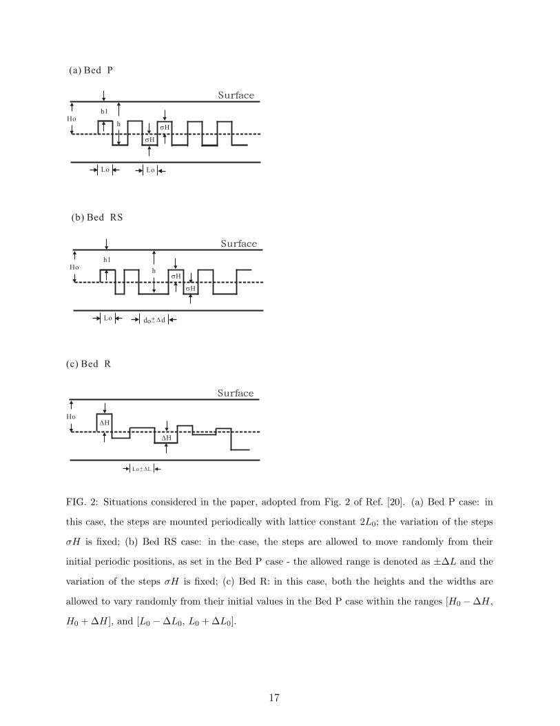
FIG. 2: Situations considered in the paper, adopted from Fig. 2 of Ref. [20]. (a) Bed P case: in

this case, the steps are mounted periodically with lattice constant 2L0; the variation of the steps

σH is fixed; (b) Bed RS case: in the case, the steps are allowed to move randomly from their

initial periodic positions, as set in the Bed P case - the allowed range is denoted as ±∆L and the

variation of the steps σH is fixed; (c) Bed R: in this case, both the heights and the widths are

allowed to vary randomly from their initial values in the Bed P case within the ranges [H0 −∆H,

H0 +∆H], and [L0 −∆L0, L0 +∆L0].

17

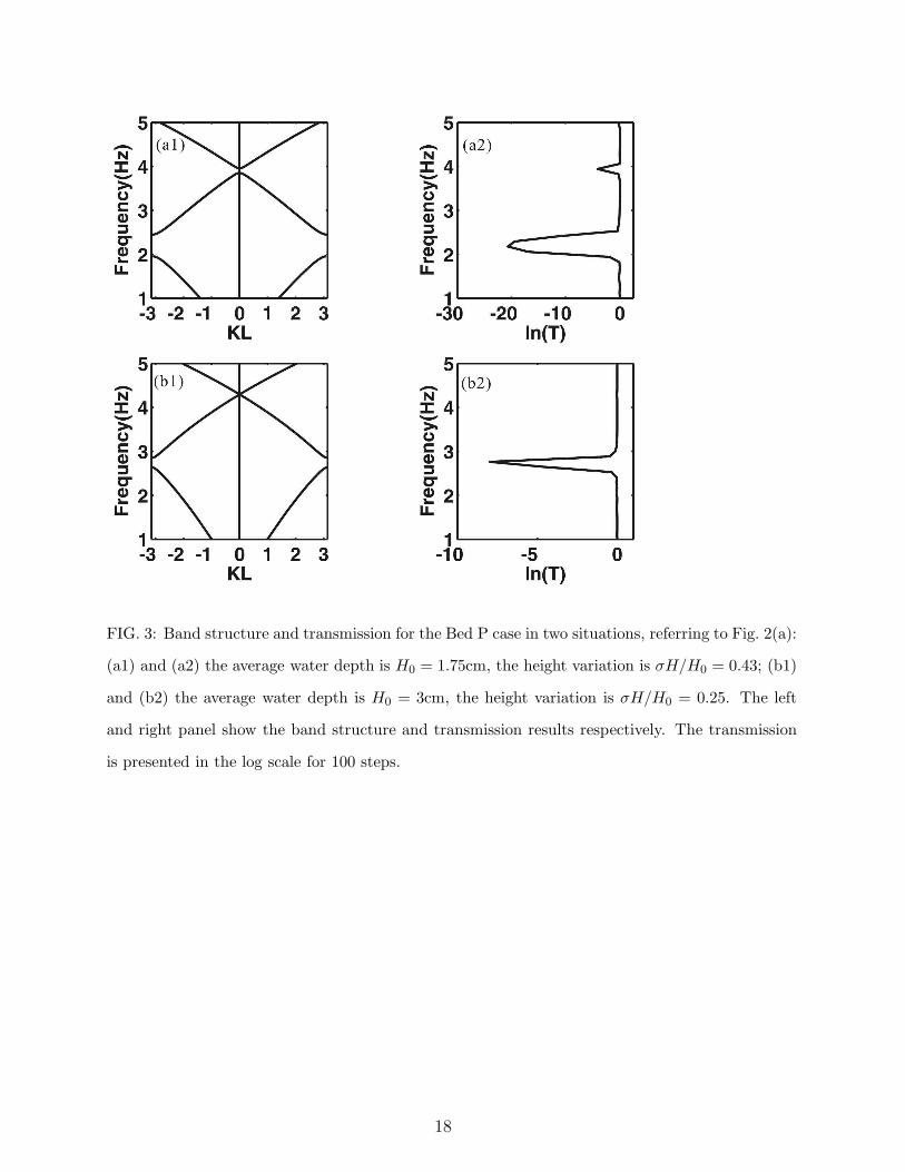
FIG. 3: Band structure and transmission for the Bed P case in two situations, referring to Fig. 2(a):

(a1) and (a2) the average water depth is H0 = 1.75cm, the height variation is σH/H0 = 0.43; (b1)

and (b2) the average water depth is H0 = 3cm, the height variation is σH/H0 = 0.25. The left

and right panel show the band structure and transmission results respectively. The transmission

is presented in the log scale for 100 steps.

18

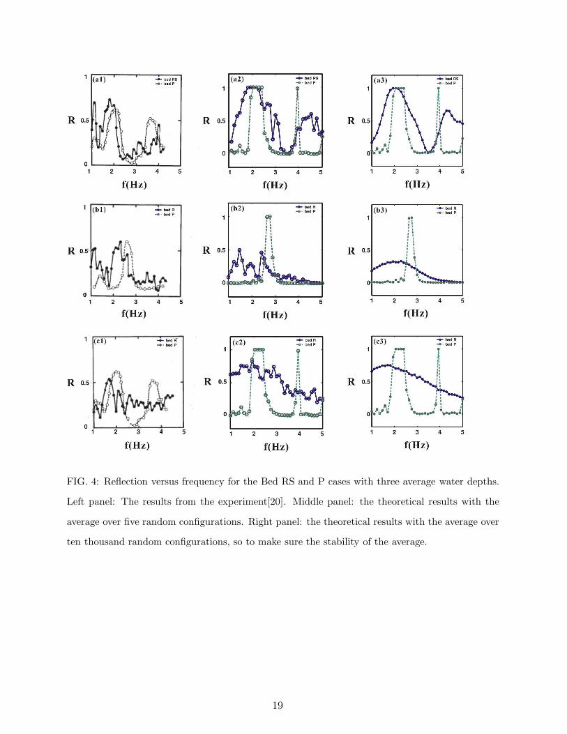
FIG. 4: Reflection versus frequency for the Bed RS and P cases with three average water depths.

Left panel: The results from the experiment[20]. Middle panel: the theoretical results with the

average over five random configurations. Right panel: the theoretical results with the average over

ten thousand random configurations, so to make sure the stability of the average.

19

FIG. 5: Localization length versus frequency for the Bed R case. The experimental results are

shown in the inset figure. The five black dots denote the results from an averaging over five

random configurations.

20

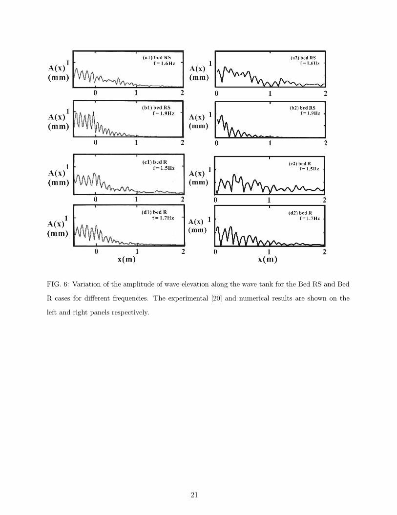
FIG. 6: Variation of the amplitude of wave elevation along the wave tank for the Bed RS and Bed

R cases for different frequencies. The experimental [20] and numerical results are shown on the

left and right panels respectively.

21

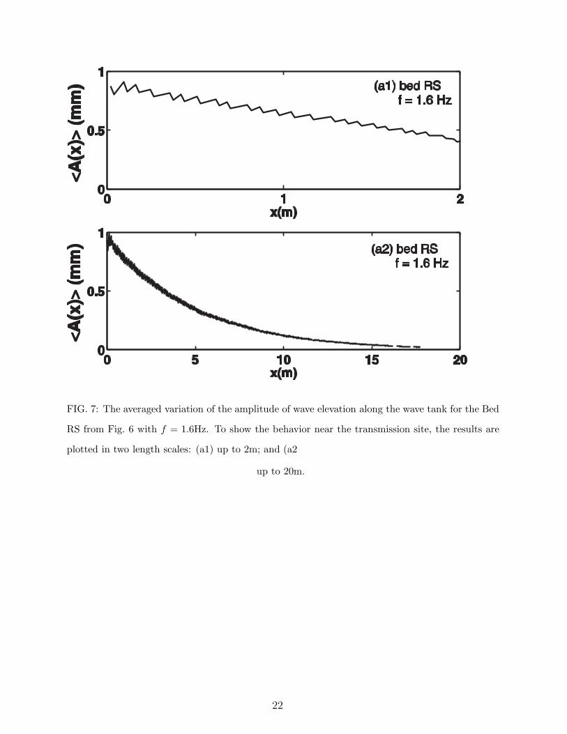
FIG. 7: The averaged variation of the amplitude of wave elevation along the wave tank for the Bed

RS from Fig. 6 with f = 1.6Hz. To show the behavior near the transmission site, the results are

plotted in two length scales: (a1) up to 2m; and (a2

up to 20m.

22