Embed Size (px)
Citation preview

arX
iv:1
503.
0585
8v2
[m
ath.
CO
] 1
1 Fe
b 20
16
MERIT FACTORS OF POLYNOMIALS DERIVED
FROM DIFFERENCE SETS
CHRISTIAN GUNTHER AND KAI-UWE SCHMIDT
Abstract. The problem of constructing polynomials with all coeffi-cients 1 or −1 and large merit factor (equivalently with small L4 normon the unit circle) arises naturally in complex analysis, condensed matterphysics, and digital communications engineering. Most known construc-tions arise (sometimes in a subtle way) from difference sets, in particularfrom Paley and Singer difference sets. We consider the asymptotic meritfactor of polynomials constructed from other difference sets, providingthe first essentially new examples since 1991. In particular we prove ageneral theorem on the asymptotic merit factor of polynomials arisingfrom cyclotomy, which includes results on Hall and Paley difference setsas special cases. In addition, we establish the asymptotic merit fac-tor of polynomials derived from Gordon-Mills-Welch difference sets andSidelnikov almost difference sets, proving two recent conjectures.
1. Introduction
The problem of constructing polynomials having all coefficients in the set{−1, 1} (frequently called Littlewood polynomials) with small Lα norm onthe complex unit circle arises naturally in complex analysis [27], [28], [5], [11],condensed matter physics [3], and the design of sequences for communica-tions devices [13], [2].
Recall that, for 1 ≤ α <∞, the Lα norm on the unit circle of a polynomialf ∈ C[z] is
‖f‖α =
(
1
2π
∫ 2π
0
∣
∣f(eiφ)∣
∣
αdφ
)1/α
.
The L4 norm has received particular attention because it is easier to calculatethan most other Lα norms. Specifically, the L4 norm of f ∈ C[z] is exactly
the sum of the squared magnitudes of the coefficients of f(z)f(z−1). It iscustomary (see [5], for example) to measure the smallness of the L4 normof a polynomial f by its merit factor F (f), defined by
F (f) =‖f‖42
‖f‖44 − ‖f‖42,
provided that the denominator is nonzero. Note that, if f is a Littlewoodpolynomial of degree n − 1, then ‖f‖2 =
√n and so a large merit factor
means that the L4 norm is small.
Date: 20 April 2015 (revised 11 February 2016).The authors are supported by German Research Foundation (DFG).

2 CHRISTIAN GUNTHER AND KAI-UWE SCHMIDT
We note that Golay’s original equivalent definition [13] of the merit factorinvolves the aperiodic autocorrelations (which are precisely the coefficients
of f(z)f(z−1)) of the sequence formed by the coefficients of f .Besides continuous progress on the merit factor problem in the last fifty
years (see [18], [16], [6] for surveys and [19] for a brief review of more recentwork), modulo generalisations and variations, only three nontrivial familiesof Littlewood polynomials are known, for which we can compute the asymp-totic merit factor. These are: Rudin-Shapiro polynomials and polynomialswhose coefficients are derived either from multiplicative or additive charac-ters of finite fields. As shown by Littlewood [28], Rudin-Shapiro polynomialsare constructed recursively in such a way that their merit factor satisfies asimple recurrence, which gives an asymptotic value of 3. The largest asymp-totic merit factors that have been obtained from the other two families equalcubic algebraic numbers 6.342061 . . . and 3.342065 . . . , respectively [20], [19](see Corollary 2.4 and Theorem 2.1 in this paper for precise statements).
The latter polynomials are closely related to classical difference sets,namely Paley and Singer difference sets. Recall that a difference set withparameters (n, k, λ) is a k-subset D of a finite group G of order n such thatthe k(k− 1) nonzero differences of elements in D hit every nonzero elementof G exactly λ times (so that k(k− 1) = λ(n− 1)). We are interested in thecase that the group G is cyclic. In this case, we fix a generator θ of G andassociate with a subset D of G the Littlewood polynomial
(1) fr,t(z) =
t−1∑
j=0
1D(θj+r)zj ,
where r and t are integers with t ≥ 0 and
1D(y) =
{
1 for y ∈ D
−1 for y ∈ G \D.If n is the group order, then f0,n captures the information about D. We callthis polynomial a characteristic polynomial of D (which is unique up to thechoice of θ) and the polynomials fr,n shifted characteristic polynomials.
The results of this paper are mainly motivated by the 1991 paper ofJensen, Jensen, and Høholdt [21], in which the authors asked for the meritfactor of polynomials derived from families of difference sets. It was shownin [21] that, among the known families of difference sets, only those withHadamard parameters, namely
(4h − 1, 2h− 1, h− 1)
for a positive integer h, can give a nonzero asymptotic merit factor for theirshifted characteristic polynomials. As of 1991, five families of such differencesets were known [21]:
(A) Paley difference sets,(B) Singer difference sets,

MERIT FACTORS OF POLYNOMIALS DERIVED FROM DIFFERENCE SETS 3
(C) Twin-prime difference sets,(D) Gordon-Mills-Welch difference sets,(E) Hall difference sets.
While in the first three cases, the asymptotic merit factors of the shiftedcharacteristic polynomials have been determined in [17] and [21] and thoseof the more general polynomials (1) in [20] and [19], the last two cases wereleft as open problems in [21]. More specifically, the asymptotic merit factorof the polynomials derived from a subclass of the Gordon-Mills-Welch dif-ference sets is subject to a conjecture [19, Conjecture 7.1]. In this paper, weprove this conjecture and solve the problems concerning Gordon-Mills-Welchand Hall difference sets posed in [21] (see Theorem 2.1 and Corollary 2.6,respectively). In addition, we obtain the asymptotic merit factor of poly-nomials related to a construction of Sidelnikov [30] (see also [25]). Thisexplains numerical observations in [15] and proves in the affirmative [19,Conjecture 7.2].
In fact, the result for Hall difference sets arises from a much more generaltheorem concerning polynomials derived from cyclotomy (see Theorem 2.3).This result considers polynomials constructed from subsets of Fp obtained byjoining m/2 of the m cyclotomic classes of (even) order m, where m satisfiesp ≡ 1 (mod m). The cases m ∈ {2, 4, 6} are examined in detail. For m = 2,we obtain the asymptotic merit factor of polynomials arising from Paleydifference sets (see Corollary 2.4), which is the main result of [20]. Form = 4,we obtain the asymptotic merit factor of polynomials arising from Ding-Helleseth-Lam almost difference sets [10] (see Corollary 2.5). For m = 6,we obtain, among other things, the asymptotic merit factor of polynomialsarising from Hall difference sets (see Corollary 2.6).
Some comments on our result for Gordon-Mills-Welch difference sets fol-low. In the cyclic case, such sets have paramaters
(2m − 1, 2m−1 − 1, 2m−2 − 1),
which are typically called Singer parameters. The Gordon-Mills-Welch con-struction produces difference sets in a cyclic group G of order 2m − 1 fromdifference sets with Singer parameters in a subgroup of G. Hence this con-struction is very general and can in particular be iterated. Our result onGordon-Mills-Welch difference sets (Theorem 2.1) requires no knowledgeabout the smaller difference sets that are used as building blocks. ThusSinger, Paley, or Hall difference sets (in groups whose order is a Mersennenumber) can be used as building blocks. In addition, since 1991, furtherfamilies of difference sets in cyclic groups with Singer parameters have beenfound:
(F) Maschietti difference sets [29],(G) Dillon-Dobbertin difference sets [9],(H) No-Chung-Yun difference sets [9].
4 CHRISTIAN GUNTHER AND KAI-UWE SCHMIDT
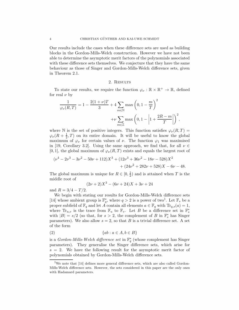
Our results include the cases when these difference sets are used as buildingblocks in the Gordon-Mills-Welch construction. However we have not beenable to determine the asymptotic merit factors of the polynomials associatedwith these difference sets themselves. We conjecture that they have the samebehaviour as those of Singer and Gordon-Mills-Welch difference sets, givenin Theorem 2.1.
2. Results
To state our results, we require the function ϕν : R × R+ → R, defined
for real ν by
1
ϕν(R,T )= 1− 2(1 + ν)T
3+ 4
∑
m∈N
max
(
0, 1 − m
T
)2
+ν∑
m∈Z
max
(
0, 1 −∣
∣
∣
∣
1 +2R−m
T
∣
∣
∣
∣
)2
,
where N is the set of positive integers. This function satisfies ϕν(R,T ) =ϕν(R + 1
2 , T ) on its entire domain. It will be useful to know the globalmaximum of ϕν for certain values of ν. The function ϕ1 was maximisedin [19, Corollary 3.2]. Using the same approach, we find that, for all ν ∈[0, 1], the global maximum of ϕν(R,T ) exists and equals the largest root of
(ν4 − 2ν3 − 3ν2 − 50ν + 112)X3 + (12ν3 + 36ν2 − 18ν − 528)X2
+ (24ν2 + 282ν + 528)X − 6ν − 48.
The global maximum is unique for R ∈ [0, 12) and is attained when T is themiddle root of
(2ν + 2)X3 − (6ν + 24)X + 3ν + 24
and R = 3/4 − T/2.We begin with stating our results for Gordon-Mills-Welch difference sets
[14] whose ambient group is F∗q, where q > 2 is a power of two1. Let Fs be a
proper subfield of Fq and let A contain all elements a ∈ Fq with Trq,s(a) = 1,where Tru,v is the trace from Fu to Fv. Let B be a difference set in F
∗s
with |B| = s/2 (so that, for s > 2, the complement of B in F∗s has Singer
parameters). We also allow s = 2, so that B is a trivial difference set. A setof the form
(2) {ab : a ∈ A, b ∈ B}is a Gordon-Mills-Welch difference set in F
∗q (whose complement has Singer
parameters). They generalise the Singer difference sets, which arise fors = 2. We have the following result for the asymptotic merit factor ofpolynomials obtained by Gordon-Mills-Welch difference sets.
1We note that [14] defines more general difference sets, which are also called Gordon-Mills-Welch difference sets. However, the sets considered in this paper are the only oneswith Hadamard parameters.

MERIT FACTORS OF POLYNOMIALS DERIVED FROM DIFFERENCE SETS 5
Theorem 2.1. Let q > 2 be a power of two and let f be a characteristicpolynomial of a Gordon-Mills-Welch difference set in F
∗q. Let T > 0 be real.
If t/q → T , then F (fr,t) → ϕ0(0, T ) as q → ∞.
In the particular case of Singer difference sets, Theorem 2.1 reduces to [19,Theorem 2.2 (i)]. The case that the Gordon-Mills-Welch difference sets inTheorem 2.1 are of the form (2) when B is a Singer difference set proves [19,Conjecture 7.1]2.
Next we consider subsets of F∗q for an odd prime power q, which are related
to a construction of Sidelnikov [30]. We call a set of the form
(3) {x ∈ F∗q : x+ 1 is zero or a square in F
∗q}
a Sidelnikov set in F∗q. Such a set gives rise to a so-called almost difference
set [1, Theorem 4]. We have the following result for the asymptotic meritfactor of the associated polynomials, proving [19, Conjecture 7.2].
Theorem 2.2. Let q be an odd prime power and let f be a characteristicpolynomial of a Sidelnikov set in F
∗q. Let T > 0 be real. If t/q → T , then
F (fr,t) → ϕ0(0, T ) as q → ∞.
The maximum asymptotic merit factor that can be obtained in Theo-rems 2.1 and 2.2 is 3.342065 . . . , the largest root of
7X3 − 33X2 + 33X − 3.
Next we construct Littlewood polynomials using cyclotomy. Let m be apositive integer and let p be a prime satisfying p ≡ 1 (mod m). Let ω be afixed primitive element in Fp. Let C0 be the set of m-th powers in F
∗p and
write Cs = ωsC0 for s ∈ Z. The sets C0, C1, . . . , Cm−1 partition F∗p and are
called the cyclotomic classes of Fp of order m.We construct subsets D of the additive group Fp by joining some of these
classes. This method provides a rich source of difference sets (see [23] for asurvey). We may take 1 as a generator for Fp, in which case the polynomialsassociated with D are
fr,t(z) =t−1∑
j=0
1D(j + r)zj
and a characteristic polynomial is f0,p (this is no loss of generality; if thegenerator is v, then replace D by v−1D). It follows from [21, Theorem 2.1]that the shifted characteristic polynomials associated with D have a nonzeroasymptotic merit factor only if |D|/p approaches 1/2 as p → ∞, thus mmust be even and D must be a union of m/2 cyclotomic classes. Twofamilies of difference sets arise in this way, namely the Paley difference sets
2Conjecture 7.1 of [19] also involves “negaperiodic” and “periodic” extensions of thepolynomials associated with Gordon-Mills-Welch difference sets. The corresponding as-sertions can be obtained as direct consequences of Proposition 5.3 and [19, Theorem 4.2],but are omitted here for the sake of simplicity.

6 CHRISTIAN GUNTHER AND KAI-UWE SCHMIDT
for m = 2 and the Hall difference sets for m = 6 [22, Theorem 2.2]. If D isa union of m/2 cyclotomic classes of order m, then |D| = (p− 1)/2, so if Dis a difference set, then it must have Hadamard parameters. Equivalently,|(D+u)∩D| = (p−3)/4 for every u ∈ F
∗p. Our next theorem applies not only
to such difference sets, but requires this condition to hold asymptotically (ina precise sense).
Theorem 2.3. Let m be an even positive integer and let S be an m/2-element subset of {0, 1, . . . ,m − 1}. Let p take values in an infinite set ofprimes satisfying p ≡ 1 (mod m). Let D be the union of the m/2 cyclotomicclasses Cs with s ∈ S of Fp of order m and suppose that, as p→ ∞,
(4)(log p)3
p2
∑
u∈F∗
p
(
∣
∣(D + u) ∩D∣
∣− p
4
)2
→ 0.
Let f be a characteristic polynomial of D and let R and T > 0 be real. Ifr/p→ R and t/p→ T , then the following hold as p→ ∞:
(i) If p−1m is even for every p, then F (fr,t) → ϕ1(R,T ).
(ii) If p−1m is odd for every p, then F (fr,t) → ϕν(R,T ), where ν = (4Nm −1)2
andN =
∣
∣{(s, s′) ∈ S × S : s− s′ = m/2}∣
∣.
Several remarks on Theorem 2.3 follow. It is readily verified that ν inTheorem 2.3 satisfies ν ∈ [0, 1]. The condition (4) is essentially necessarysince
1
F (f)≥ 8
p2
∑
u∈F∗
p
(
∣
∣(D + u) ∩D∣
∣− p− 2
4
)2
.
This can be deduced from the proof of Theorem 2.3 and the inequality
‖f‖44 ≥1
2p
∑
k∈Fp
|f(e2πik/p)|4 + p2
2,
which can be obtained from [17, (2.3)] with an extra step involving theCauchy-Schwarz inequality. In fact, this is a refinement of the Marcinkiewicz-Zygmund inequality [32, Chapter X, Theorem 7.5] for the L4 norm.
The condition (4) can be checked using the cyclotomic numbers of or-der m, which are the m2 numbers
|(Ci + 1) ∩ Cj|for 0 ≤ i, j < m. These numbers are known explicitly for all even m ≤ 20and for m = 24 (see [4, p. 152] for a list of references). Also note thatthe conclusion of Theorem 2.3 remains unchanged if we replace S by h+ Sreduced modulo m for an integer h (which changes D to ωhD).
We now consider in detail the cases m ∈ {2, 4, 6} of Theorem 2.3. Ifm = 2, then D consists of either the squares or the nonsquares of F∗
p. Inboth cases, D is a Paley difference set for p ≡ 3 (mod 4). As remarked

MERIT FACTORS OF POLYNOMIALS DERIVED FROM DIFFERENCE SETS 7
above, we can assume without loss of generality that D is the set of squaresin F
∗p. Then we have (see [4, Theorem 2.2.2], for example)
4 |(D + u) ∩D| ={
p− 4− (−1)p−12 for u a square in F
∗p
p− 2 + (−1)p−12 for u a nonsquare in F
∗p.
Noting that ν = 1 for m = 2, we obtain the following corollary, which isessentially the main result of [20] (see also [19, Theorem 2.1]).
Corollary 2.4. Let p take values in an infinite set of odd primes, let Dbe either the set of squares or the set of nonsquares of F∗
p and let f be acharacteristic polynomial of D. Let R and T > 0 be real. If r/p → R andt/p→ T , then F (fr,t) → ϕ1(R,T ) as p→ ∞.
We now look at the case m = 4. Here, we only need to consider two casesfor joining two cyclotomic classes of order four, namely C0∪C2 and C0∪C1.The first case brings us back to m = 2. When p is of the form x2 + 4 forx ∈ Z and (p− 1)/4 is odd, the second case gives rise to the Ding-Helleseth-Lam almost difference sets [10, Theorem 4]. By inspecting the cyclotomicnumbers of order four (see Section 7), we obtain the following.
Corollary 2.5. Let p take values in an infinite set of primes of the form x2+4y2 for x, y ∈ Z such that y2(log p)3/p → 0 as p → ∞. Let D be the unionof two cyclotomic classes of Fp of order four and let f be a characteristicpolynomial of D. Let R and T > 0 be real. If r/p → R and t/p → T , thenF (fr,t) → ϕ1(R,T ) as p→ ∞.
Recall from elementary number theory that primes of the form x2+4y2 forx, y ∈ Z are exactly the primes that are congruent to 1 modulo 4. It is alsoknown [7] that there are infinitely many primes satisfying the hypothesis ofthe corollary.
The case m = 6 is the first situation, where different limiting functionsoccur. In this case, there are four different sets D to consider, namely
(5) C0 ∪C2 ∪ C4, C0 ∪ C1 ∪ C2, C0 ∪C1 ∪ C3, C0 ∪ C1 ∪C4.
Again, the first set brings us back to m = 2. When p is of the form x2 +27 for x ∈ Z and (p − 1)/6 is odd, then either the third or the fourthset in (5) gives rise to Hall difference sets [22] (the choice depends on theprimitive element ω). We shall see that Theorem 2.3 gives two possiblelimiting functions for the sixth cyclotomic classes, which is our motivationfor the following definition. Let D be a union of three cyclotomic classes oforder six. If there is a γ ∈ F
∗p such that γD equals one of the first two sets
in (5), then we say that D is of Paley type. Otherwise, we say that D is ofHall type.
Corollary 2.6. Let p take values in an infinite set of primes of the formx2 + 27y2 for x, y ∈ Z such that y2(log p)3/p → 0 as p → ∞. Let Dbe the union of three cyclotomic classes of Fp of order six and let f be a
8 CHRISTIAN GUNTHER AND KAI-UWE SCHMIDT
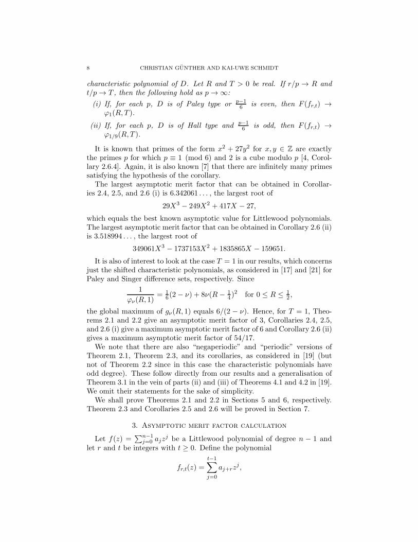
characteristic polynomial of D. Let R and T > 0 be real. If r/p → R andt/p→ T , then the following hold as p→ ∞:
(i) If, for each p, D is of Paley type or p−16 is even, then F (fr,t) →
ϕ1(R,T ).
(ii) If, for each p, D is of Hall type and p−16 is odd, then F (fr,t) →
ϕ1/9(R,T ).
It is known that primes of the form x2 + 27y2 for x, y ∈ Z are exactlythe primes p for which p ≡ 1 (mod 6) and 2 is a cube modulo p [4, Corol-lary 2.6.4]. Again, it is also known [7] that there are infinitely many primessatisfying the hypothesis of the corollary.
The largest asymptotic merit factor that can be obtained in Corollar-ies 2.4, 2.5, and 2.6 (i) is 6.342061 . . . , the largest root of
29X3 − 249X2 + 417X − 27,
which equals the best known asymptotic value for Littlewood polynomials.The largest asymptotic merit factor that can be obtained in Corollary 2.6 (ii)is 3.518994 . . . , the largest root of
349061X3 − 1737153X2 + 1835865X − 159651.
It is also of interest to look at the case T = 1 in our results, which concernsjust the shifted characteristic polynomials, as considered in [17] and [21] forPaley and Singer difference sets, respectively. Since
1
ϕν(R, 1)= 1
6(2− ν) + 8ν(R− 14 )
2 for 0 ≤ R ≤ 12 ,
the global maximum of gν(R, 1) equals 6/(2 − ν). Hence, for T = 1, Theo-rems 2.1 and 2.2 give an asymptotic merit factor of 3, Corollaries 2.4, 2.5,and 2.6 (i) give a maximum asymptotic merit factor of 6 and Corollary 2.6 (ii)gives a maximum asymptotic merit factor of 54/17.
We note that there are also “negaperiodic” and “periodic” versions ofTheorem 2.1, Theorem 2.3, and its corollaries, as considered in [19] (butnot of Theorem 2.2 since in this case the characteristic polynomials haveodd degree). These follow directly from our results and a generalisation ofTheorem 3.1 in the vein of parts (ii) and (iii) of Theorems 4.1 and 4.2 in [19].We omit their statements for the sake of simplicity.
We shall prove Theorems 2.1 and 2.2 in Sections 5 and 6, respectively.Theorem 2.3 and Corollaries 2.5 and 2.6 will be proved in Section 7.
3. Asymptotic merit factor calculation
Let f(z) =∑n−1
j=0 ajzj be a Littlewood polynomial of degree n − 1 and
let r and t be integers with t ≥ 0. Define the polynomial
fr,t(z) =
t−1∑
j=0
aj+rzj ,

MERIT FACTORS OF POLYNOMIALS DERIVED FROM DIFFERENCE SETS 9
where we extend the definition of aj so that aj+n = aj for all j ∈ Z. Write
ǫk = e2πik/n. From [19] it is known that F (fr,t) depends only on the functionLf : (Z/nZ)3 → Z, defined by
Lf (a, b, c) =1
n3
∑
k∈Z/nZ
f(ǫk)f(ǫk+a)f(ǫk+b)f(ǫk+c).
Define the functions In, Jn : (Z/nZ)3 → Z by
In(a, b, c) =
{
1 if (c = a and b = 0) or (b = a and c = 0),
0 otherwise
and
Jn(a, b, c) =
{
1 if a = 0 and b = c 6= 0,
0 otherwise
and, for even n, the function Kn : (Z/nZ)3 → Z by
Kn(a, b, c) =
{
1 if a = n/2 and b = c+ n/2 and bc 6= 0,
0 otherwise.
In order to prove Theorems 2.1, 2.2, and 2.3 we shall show that the corre-sponding function Lf is well approximated by either In + νJn for an appro-priate real ν or by In+Kn and then apply one of the following two theorems.Our first theorem is a slight generalisation of Theorems 4.1 (i) and 4.2 (i)of [19], which arise by setting ν = 1 and ν = 0, respectively. This theoremcan be proved by applying straightforward modifications to the proof of [19,Theorem 4.1].
Theorem 3.1. Let ν be a real number and let n take values in an infinite setof positive integers. For each n, let f be a Littlewood polynomial of degreen− 1 and suppose that, as n→ ∞,
(log n)3 maxa,b,c∈Z/nZ
∣
∣Lf (a, b, c) − (In(a, b, c) + νJn(a, b, c))∣
∣→ 0.
Let R and T > 0 be real. If r/n→ R and t/n→ T , then F (fr,t) → ϕν(R,T )as n→ ∞.
There is a similar generalisation of parts (ii) and (iii) of Theorems 4.1and 4.2 in [19], which we do not consider in this paper.
Our second theorem is a more subtle modification of Theorem 4.1 (i)in [19]. We include a proof that highlights the required modifications of theproof of [19, Theorem 4.1 (i)].
Theorem 3.2. Let n take values in an infinite set of even positive integers.For each n, let f be a Littlewood polynomial of degree n − 1 and supposethat, as n→ ∞,
(6) (log n)3 maxa,b,c∈Z/nZ
∣
∣Lf (a, b, c) − (In(a, b, c) +Kn(a, b, c))∣
∣→ 0.
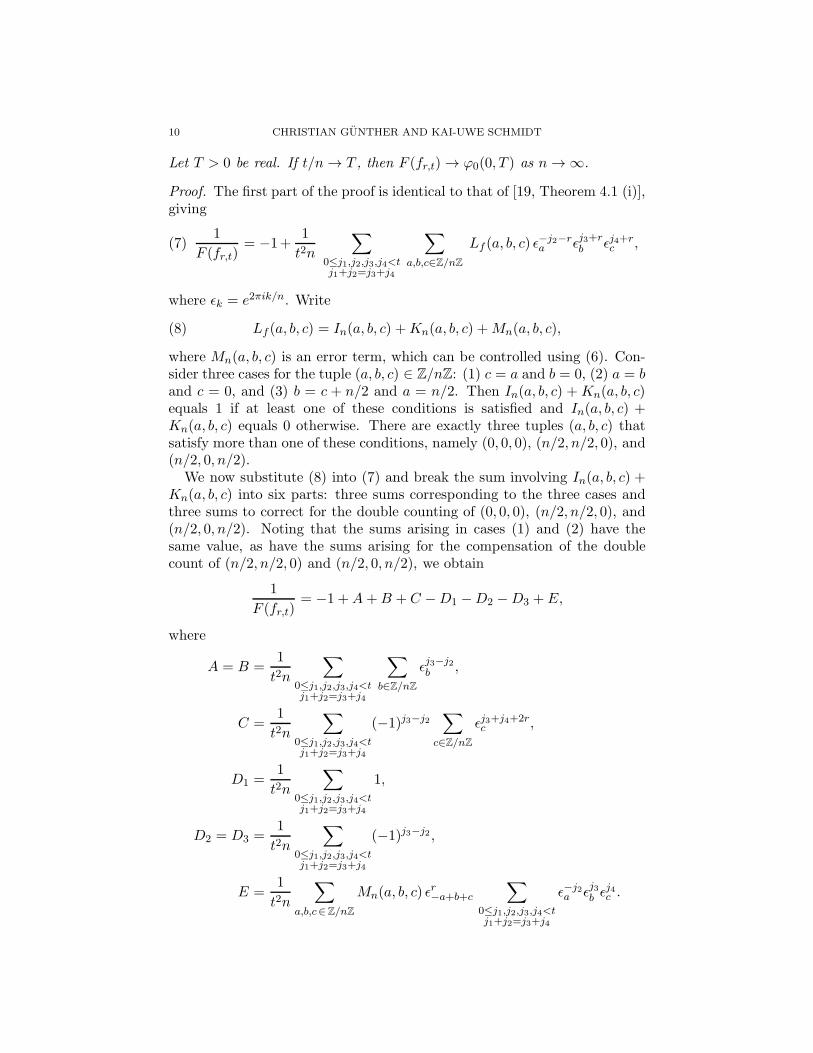
10 CHRISTIAN GUNTHER AND KAI-UWE SCHMIDT
Let T > 0 be real. If t/n→ T , then F (fr,t) → ϕ0(0, T ) as n→ ∞.
Proof. The first part of the proof is identical to that of [19, Theorem 4.1 (i)],giving
(7)1
F (fr,t)= −1+
1
t2n
∑
0≤j1,j2,j3,j4<tj1+j2=j3+j4
∑
a,b,c∈Z/nZ
Lf (a, b, c) ǫ−j2−ra ǫj3+r
b ǫj4+rc ,
where ǫk = e2πik/n. Write
(8) Lf (a, b, c) = In(a, b, c) +Kn(a, b, c) +Mn(a, b, c),
where Mn(a, b, c) is an error term, which can be controlled using (6). Con-sider three cases for the tuple (a, b, c) ∈ Z/nZ: (1) c = a and b = 0, (2) a = band c = 0, and (3) b = c + n/2 and a = n/2. Then In(a, b, c) +Kn(a, b, c)equals 1 if at least one of these conditions is satisfied and In(a, b, c) +Kn(a, b, c) equals 0 otherwise. There are exactly three tuples (a, b, c) thatsatisfy more than one of these conditions, namely (0, 0, 0), (n/2, n/2, 0), and(n/2, 0, n/2).
We now substitute (8) into (7) and break the sum involving In(a, b, c) +Kn(a, b, c) into six parts: three sums corresponding to the three cases andthree sums to correct for the double counting of (0, 0, 0), (n/2, n/2, 0), and(n/2, 0, n/2). Noting that the sums arising in cases (1) and (2) have thesame value, as have the sums arising for the compensation of the doublecount of (n/2, n/2, 0) and (n/2, 0, n/2), we obtain
1
F (fr,t)= −1 +A+B + C −D1 −D2 −D3 + E,
where
A = B =1
t2n
∑
0≤j1,j2,j3,j4<tj1+j2=j3+j4
∑
b∈Z/nZ
ǫj3−j2b ,
C =1
t2n
∑
0≤j1,j2,j3,j4<tj1+j2=j3+j4
(−1)j3−j2∑
c∈Z/nZ
ǫj3+j4+2rc ,
D1 =1
t2n
∑
0≤j1,j2,j3,j4<tj1+j2=j3+j4
1,
D2 = D3 =1
t2n
∑
0≤j1,j2,j3,j4<tj1+j2=j3+j4
(−1)j3−j2 ,
E =1
t2n
∑
a,b,c∈Z/nZ
Mn(a, b, c) ǫr−a+b+c
∑
0≤j1,j2,j3,j4<tj1+j2=j3+j4
ǫ−j2a ǫj3b ǫ
j4c .

MERIT FACTORS OF POLYNOMIALS DERIVED FROM DIFFERENCE SETS 11
As in the proof of [19, Theorem 4.2], we have −1 + A + B − D1 + E →1/ϕ0(0, T ) if t/n → T . Hence it remains to show that C −D2 −D3 → 0 ift/n→ T .
Since there are contributions to the first sum in C only when j3 + j4 =mn− 2r for some m ∈ Z, we obtain
C =1
t2
∑
m∈Z
(
∑
0≤j,mn−2r−j<t
(−1)j
)2
.
Therefore we have |C| ≤ 1/(tn) and so C → 0 if t/n → T . By writingj3 = j1 +m for some m ∈ Z we find that
D2 =1
t2n
∑
m∈Z
(
∑
0≤j,j+m<t
(−1)j
)2
.
Hence |D2| ≤ 1/(tn) and therefore D2+D3 → 0 if t/n→ T . This completesthe proof. �
4. Some background on Gauss and Jacobi sums
Let χ be a multiplicative character of Fq. Throughout this paper, we usethe common convention
χ(0) =
{
0 if χ is nontrivial
1 if χ is trivial.
We define the canonical Gauss sum of χ to be
(9) G(χ) =∑
y∈F∗
q
χ(y) e2πiTrq,p(y)/p,
where p is the characteristic of Fq and Trq,p is the trace from Fq to Fp. Belowwe summarise some basic facts about such Gauss sums (see [26, Chapter 5]or [4, Chapter 1], for example).
Lemma 4.1. Let χ be a multiplicative character of Fq. Then the followinghold.
(i) G(χ) = −1 if χ is trivial.
(ii) |G(χ)| = √q if χ is nontrivial.
(iii) G(χ)G(χ) = χ(−1) q.
We also require the following deep result due to Katz [24, pp. 161–162].
Lemma 4.2. Let α1, . . . , αr, β1, . . . , βs be multiplicative characters of Fq
such that α1, . . . , αr do not arise by permuting β1, . . . , βs. Then∣
∣
∣
∣
∣
∑
χ
G(χα1) · · · G(χαr)G(χβ1) · · · G(χβs)∣
∣
∣
∣
∣
≤ max(r, s) q(r+s+1)/2,
where the sum runs over all multiplicative characters χ of Fq.

12 CHRISTIAN GUNTHER AND KAI-UWE SCHMIDT
Now let ψ and χ be multiplicative characters of Fq. The Jacobi sumcorresponding to ψ and χ is defined to be
J(ψ,χ) =∑
y∈Fq
ψ(y)χ(1 − y).
Below we summarise some basic facts about Jacobi sums (see [26, Chapter 5]or [4, Chapter 2], for example).
Lemma 4.3. Let ψ and χ be multiplicative characters of Fq. Then thefollowing hold.
(i) J(ψ,χ) = 0 if exactly one of ψ or χ is trivial.
(ii) |J(ψ,χ)| = 1 if ψ and χ are nontrivial, but ψχ is trivial.
(iii) |J(ψ,χ)| = √q if all of ψ, χ, and ψχ are nontrivial.
(iv) J(ψ,χ) q = G(ψ)G(χ)G(ψχ) if ψ and χ are nontrivial.
(v) J(ψ,χ)J(ψ,χψ) = ψ(−1)q if ψ and χ are nontrivial.
5. Gordon-Mills-Welch difference sets
In this section we prove Theorem 2.1. If D is a subset of a finite abeliangroup G and χ is a character of G, we write
χ(D) =∑
d∈D
χ(d).
The following lemma is a standard (and easily verified).
Lemma 5.1. A k-subset D of a finite abelian group G of order n is adifference set if and only if
|χ(D)|2 =k(n− k)
n− 1
for all nontrivial characters χ of G.
The following lemma gives the character values of Gordon-Mills-Welchdifference sets and in particular gives an alternative proof of the main resultof [14] (although, for simplicity, we restrict q to be even).
Lemma 5.2. Let q > 2 be a power of two and let Fs be a subfield of Fq.Let A contain all elements a ∈ Fq with Trq,s(a) = 1, let B be a subset of F∗
s,and write D = {ab : a ∈ A, b ∈ B}. Let χ be a nontrivial character of F∗
q
and let χ∗ be its restriction to F∗s. Then
χ(D) =
χ∗(B)
G(χ∗)G(χ) for χ∗ nontrivial
−χ∗(B)
sG(χ) for χ∗ trivial.
In particular, if B is a difference set in F∗s and |B| = s/2, then D is a
difference set with parameters (q − 1, q/2, q/4).
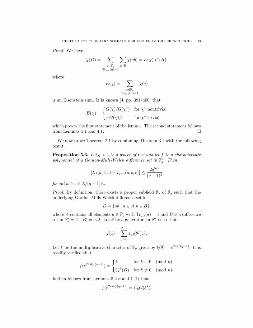
MERIT FACTORS OF POLYNOMIALS DERIVED FROM DIFFERENCE SETS 13
Proof. We have
χ(D) =∑
a∈Fq
Trq,s(a)=1
∑
b∈B
χ(ab) = E(χ)χ∗(B),
where
E(χ) =∑
a∈Fq
Trq,s(a)=1
χ(a)
is an Eisenstein sum. It is known [4, pp. 391/400] that
E(χ) =
{
G(χ)/G(χ∗) for χ∗ nontrivial
−G(χ)/s for χ∗ trivial,
which proves the first statement of the lemma. The second statement followsfrom Lemmas 5.1 and 4.1. �
We now prove Theorem 2.1 by combining Theorem 3.1 with the followingresult.
Proposition 5.3. Let q > 2 be a power of two and let f be a characteristicpolynomial of a Gordon-Mills-Welch difference set in F
∗q. Then
∣
∣Lf (a, b, c) − Iq−1(a, b, c)∣
∣ ≤ 2q5/2
(q − 1)3
for all a, b, c ∈ Z/(q − 1)Z.
Proof. By definition, there exists a proper subfield Fs of Fq such that theunderlying Gordon-Mills-Welch difference set is
D = {ab : a ∈ A, b ∈ B},where A contains all elements a ∈ Fq with Trq,s(a) = 1 and B is a differenceset in F
∗s with |B| = s/2. Let θ be a generator for F∗
q such that
f(z) =
q−2∑
j=0
1D(θj)zj .
Let ξ be the multiplicative character of Fq given by ξ(θ) = e2πi/(q−1). It isreadily verified that
f(e2πik/(q−1)) =
{
1 for k ≡ 0 (mod n)
2ξk(D) for k 6≡ 0 (mod n).
It then follows from Lemmas 5.2 and 4.1 (i) that
f(e2πik/(q−1)) = CkG(ξk),

14 CHRISTIAN GUNTHER AND KAI-UWE SCHMIDT
where Ck has unit magnitude for all k and depends only on k modulo s− 1.Therefore
(10) Lf (a, b, c) =1
(q − 1)3
∑
χ
G(χ)G(χξa)G(χξb)G(χξc) Cχ(a, b, c),
where the sum is over all multiplicative characters χ of Fq and Cχ(a, b, c)has unit magnitude. Using Lemma 4.1, we obtain
Lf (a, b, c) =
1 + q−2(q−1)2
for a = b = c = 0
1− 1(q−1)2
for {0, a} = {b, c} and a 6= 0,
which proves the desired result in the case that Iq−1(a, b, c) = 1.Now assume that {0, a} 6= {b, c}, so that Iq−1(a, b, c) = 0. We need to
show that
(11) |Lf (a, b, c)| ≤2q5/2
(q − 1)3.
Let H be the subgroup of index s − 1 of the character group of F∗q and
note that H is not the trivial group since, by assumption, s < q. ThenCχ(a, b, c) is constant when χ ranges over a coset of H. Since Cχ(a, b, c) hasunit magnitude, we find from (10) and the triangle inequality that
(12) |Lf (a, b, c)| ≤s− 1
(q − 1)3maxφ
∣
∣
∣
∣
∣
∑
χ∈H
G(χφ)G(χφξa)G(χφξb)G(χφξc)
∣
∣
∣
∣
∣
,
where the maximum is over all multiplicative characters φ of Fq. By thedefinition (9) of a Gauss sum over Fq, the inner sum can be written as
∑
w,x,y,z∈F∗
q
(−1)Trq,2(w+x+y+z) ξa(x)ξb(y)ξc(z)φ(wx
yz
)
∑
χ∈H
χ(wx
yz
)
.
For each w, x, y, z ∈ F∗q, we have
s− 1
q − 1
∑
χ∈H
χ(wx
yz
)
=1
q − 1
∑
χ
χ(wx
yz
)
,
where the sum on the right-hand side is over all multiplicative charactersof Fq, since both sides equal either 0 or 1 depending on whether wx = yz ornot. Therefore, we can rewrite the inner sum of (12) as
1
s− 1
∑
χ
G(χφ)G(χφξa)G(χφξb)G(χφξc),
where χ now runs over all multiplicative characters of Fq. The magnitude
of this expression is at most 2s−1q
5/2 by Lemma 4.2. Substitute into (12) to
conclude that (11) holds, as required. �

MERIT FACTORS OF POLYNOMIALS DERIVED FROM DIFFERENCE SETS 15
6. Sidelnikov sets
In this section we prove Theorem 2.2 by combining Theorem 3.2 with thefollowing result.
Proposition 6.1. Let q be an odd prime power and let f be a characteristicpolynomial of a Sidelnikov set in F
∗q. Then
∣
∣Lf (a, b, c) − (Iq−1(a, b, c) +Kq−1(a, b, c))∣
∣ ≤ 23q5/2
(q − 1)3
for all a, b, c ∈ Z/(q − 1)Z.
Proof. Let η be the quadratic character of Fq. By the definition of a Sidel-nikov set (3), there exists a generator θ of F∗
q such that
f(z) = zq−12 +
q−2∑
j=0
η(θj + 1)zj ,
where, as usual, η(0) = 0. Let ξ be the multiplicative character of Fq given
by ξ(θ) = e2πi/(q−1). Then we have, for all k 6≡ 0 (mod q − 1),
f(e2πik/(q−1)) = (−1)k +
q−2∑
j=0
η(θj + 1)ξk(θj)
= (−1)k +∑
y∈Fq
η(y + 1)ξk(y)
= (−1)k + ξk(−1)∑
y∈Fq
η(y)ξk(1− y)
= (−1)k(1 + J(η, ξk)).
On the other hand we have f(1) = 1− η(1) = 0. Therefore
(13) Lf (a, b, c) =(−1)a+b+c
(q − 1)3
∑
χ
J(η, χ)J(η, χξa)J(η, χξb)J(η, χξc) + ∆,
where the sum is over all multiplicative characters χ of Fq and |∆| ≤15q3/2/(q−1)2, using Lemma 4.3. If one of b and c equals a and the other iszero, then by Lemma 4.3 the sum in (13) is between (q− 5)q2 and (q− 2)q2.If a = (q − 1)/2 and b = c + (q − 1)/2, then ξa = η and ξb = ξcη and byLemma 4.3 (in particular (v)) the sum (13) is again at least (q − 5)q2 andat most (q − 2)q2. Since
(q − 5)q2
(q − 1)3= 1− 2q2 + 3q − 1
(q − 1)3,
this establishes the cases in which either Iq−1(a, b, c) orKq−1(a, b, c) equals 1.Now assume that (a, b, c) is such that Iq−1(a, b, c) and Kq−1(a, b, c) are
both zero. Equivalently, the multisets
(14) {ξ0, ξa, ξbη, ξcη} and {η, ξaη, ξb, ξc}

16 CHRISTIAN GUNTHER AND KAI-UWE SCHMIDT
are distinct. Use Lemmas 4.3 and 4.1 to see that the sum in (13) equals
(15)1
q2
∑
χ
G(χ)G(χξa)G(χηξb)G(χηξc)G(χη)G(χηξa)G(χξb)G(χξc)
plus an error term of magnitude at most 4q3/2, where the sum is over allmultiplicative characters χ of Fq. Since the multisets (14) are distinct, we
can apply Lemma 4.2 to see that (15) is at most 4q5/2. This shows that
|Lf (a, b, c)| ≤23q5/2
(q − 1)3,
as required. �
7. Cyclotomic constructions
In this section we prove Theorem 2.3 and Corollaries 2.5 and 2.6. Weshall use the following notation. Let m be an even positive integer and let pbe a prime satisfying p ≡ 1 (mod m). Let ω be a primitive element of Fp
and let C0, C1, . . . , Cm−1 be the cyclotomic classes of Fp of order m withrespect to ω. Let S be an m/2-element subset of {0, 1, . . . ,m − 1} and letD be the union of the m/2 cyclotomic classes Cs with s ∈ S. Taking 1 as agenerator for the additive group of Fp, a characteristic polynomial of D is
(16) f(z) =
p−1∑
j=0
1D(j)zj .
The following lemma gives the evaluations of f at p-th roots of unity.
Lemma 7.1. Assume the notation as above and let χ be a multiplicativecharacter of Fp of order m. Then
f(e2πik/p) =2
m
m−1∑
j=1
G(χj)χj(k)∑
s∈S
χj(ωs)− 1.
Proof. Since f(1) = |D|− |Fp \D| = −1, the result holds for k ≡ 0 (mod p),so assume that k 6≡ 0 (mod p). By definition we have
f(e2πik/p) =∑
y∈D
e2πiky/p −∑
y∈Fp\D
e2πiky/p
= 2∑
y∈D
e2πiky/p −∑
y∈Fp
e2πiky/p
= 2∑
y∈D
e2πiky/p
= 2∑
s∈S
∑
y∈Cs
e2πiky/p.

MERIT FACTORS OF POLYNOMIALS DERIVED FROM DIFFERENCE SETS 17
Writing h = p−1m , the inner sum can be written as
∑
y∈Cs
e2πiky/p =
h−1∑
j=0
e2πikωmj+s/p
=1
m
∑
y∈Fp
e2πik ωsym/p − 1
.
Since∑m−1
j=0 χj(y) equals m if y is an m-th power and equals zero otherwise,we have, for each a ∈ F
∗p,
∑
y∈Fp
e2πiaym/p =
∑
y∈Fp
e2πiay/pm−1∑
j=0
χj(y)
=m−1∑
j=0
∑
y∈Fp
e2πiy/p χj(y)χj(a).
For j = 0, the inner sum equals zero, so we can let the outer sum start withj = 1. Then all involved multiplicative characters are nontrivial and we canrestrict the summation range of the inner sum to F
∗p. Therefore
∑
y∈Fp
e2πiaym/p =
m−1∑
j=1
G(χj)χj(a),
which gives the desired result. �
Our next result estimates Lf for f given in (16) at all points, but (0, 0, 0).
Proposition 7.2. With the notation as above, we have∣
∣Lf (a, b, c) − (Ip(a, b, c) + νJp(a, b, c))∣
∣ ≤ 18(m− 1)4p−1/2
for all a, b, c ∈ Z/pZ with (a, b, c) 6= (0, 0, 0), where
ν =
{
1 for p−1m even
(4Nm − 1)2 for p−1m odd
and
N =∣
∣{(s, s′) ∈ S × S : s− s′ = m/2}∣
∣.
Proof. Let χ be a multiplicative character of Fp of order m and write
K(χj) =2
m
∑
s∈S
χj(ωs).
From Lemma 7.1 we find that
(17) f(e2πik/p) =
m−1∑
j=1
G(χj)K(χj)χj(k)− 1.

18 CHRISTIAN GUNTHER AND KAI-UWE SCHMIDT
Hence Lf (a, b, c) equals
(18)1
p3
m−1∑
j1,j2,j3,j4=1
G(χj1)G(χj2)G(χj3)G(χj4)K(χj1)K(χj2)K(χj3)K(χj4)
×∑
k∈Fp
χj1(k)χj2(k + a)χj3(k + b)χj4(k + c) + ∆,
where |∆| ≤ 15(m − 1)4p−1/2, using that the magnitude of the sum on theright-hand side of (17) is at most (m− 1)p1/2 by Lemma 4.1. First considerthe case that b = 0 and c = a 6= 0, so that Ip(a, b, c) = 1 and Jp(a, b, c) = 0.Then the inner sum in (18) is
∑
k∈Fp
χj3−j1(k)χj4−j2(k + a).
This sum either has magnitude at most√p by the Weil bound (see [26,
Theorem 5.41], for example) or equals p. Since a 6= 0, the latter case occursif and only if j1 ≡ j3 (mod m) and j2 ≡ j4 (mod m). Therefore Lf (a, 0, a)equals
1
p2
m−1∑
j=1
|G(χj)|2 |K(χj)|2
2
plus an error term of magnitude at most 16(m − 1)4p−1/2. Then we findfrom Lemma 4.1 and
m−1∑
j=1
∣
∣K(χj)∣
∣
2= 1
that the desired result holds for b = 0 and c = a 6= 0. The case c = 0 andb = a 6= 0 is completely analogous.
Now assume that a = 0 and c = b 6= 0, so that Ip(a, b, c) = 0 andJp(a, b, c) = 1. Then the inner sum in (18) equals
∑
k∈Fp
χj1+j2(k)χj3+j4(k + b).
As before, this sum either has magnitude at most√p or equals p, where the
latter case occurs if and only if j1 ≡ −j2 (mod m) and j3 ≡ −j4 (mod m).Hence Lf (0, b, b) equals
(19)1
p2
∣
∣
∣
∣
∣
m−1∑
j=1
G(χj)G(χj)K(χj)K(χj)
∣
∣
∣
∣
∣
2
plus an error term of magnitude at most 16(m−1)4p−1/2. From Lemma 4.1we find that (19) equals
∣
∣
∣
∣
∣
m−1∑
j=1
χj(−1) |K(χj)|2∣
∣
∣
∣
∣
2
=
(
m−1∑
j=1
(−1)j(p−1)
m
∣
∣
∣
∣
∣
2
m
∑
s∈S
e2πijs/m
∣
∣
∣
∣
∣
2)2
.

MERIT FACTORS OF POLYNOMIALS DERIVED FROM DIFFERENCE SETS 19
A standard calculation then shows that this expression equals ν. This provesthe desired result in the case that a = 0 and c = b 6= 0.
Now assume that 0, a, b, c do not form two pairs of equal elements. In thiscase, we invoke the Weil bound again to conclude that the inner sum in (18)is at most 3
√p in magnitude. Therefore we have by Lemma 4.1
|Lf (a, b, c)| ≤ 18(m− 1)4p−1/2,
which completes the proof. �
Proof of Theorem 2.3. Without loss of generality, we may choose 1 as agenerator for the additive group of Fp and take (16) as a characteristicpolynomial of D (if the generator is v, then replace D by v−1D).
We shall deduce Theorem 2.3 from Theorem 3.1. Proposition 7.2 takescare of all values of Lf (a, b, c) in the condition of Theorem 3.1, except when(a, b, c) = (0, 0, 0). We shall show that our assumption (4) takes care of thelatter case. Writing
Ru =∑
y∈Fp
1D(y)1D(y + u),
a standard calculation gives
|f(e2πik/p)|2 =∑
u∈Fp
Ru e−2πiku/p
and therefore, by Parseval’s identity,
1
p
∑
k∈Fp
|f(e2πik/p)|4 =∑
u∈Fp
R2u.
A counting argument shows that
Ru = 4 |(D + u) ∩D| − (p− 2).
Therefore, since 2|D| = p− 1, we find that Lf (0, 0, 0) equals
1
p3
∑
k∈Fp
|f(e2πik/p)|4 = 1 +1
p2
∑
u∈F∗
p
(
4 |(D + u) ∩D| − (p− 2))2.
Now our assumption (4) together with Proposition 7.2 imply that the con-dition of Theorem 3.1 is satisfied, which proves Theorem 2.3. �
Next we show how to deduce Corollaries 2.5 and 2.6 from Theorem 2.3.First consider Corollary 2.5. As explained in Section 2, we just need toconsider the case that D = C0 ∪ C1. The cyclotomic numbers of order fourhave been already determined by Gauss and can be found, for example,in [4, Theorem 2.4.1]. These numbers depend on the representation p =x2 + 4y2 and on the parity of (p − 1)/4. They also depend on the choiceof the primitive element in Fp used to define the cyclotomic classes, butthis is encapsulated in the fact that y is only unique up to sign. Using thecyclotomic numbers of order four, we obtain the numbers |(D + u) ∩ D|,

20 CHRISTIAN GUNTHER AND KAI-UWE SCHMIDT
Table 1. The numbers 4|(D+u)∩D|−(p−2) forD = C0∪C1
and primes p of the form p = x2 + 4y2.
D p−14 even p−1
4 odd
u ∈ C0 −3 + 2y −1− 2y
u ∈ C1 −3− 2y −1 + 2y
u ∈ C2 1 + 2y −1− 2y
u ∈ C3 1− 2y −1 + 2y
Table 2. The numbers 4|(D + u) ∩D| − (p − 2) for primesof the form x2 + 27y2 and (p − 1)/6 odd.
D C0 ∪ C1 ∪ C2 C0 ∪C1 ∪ C3 C0 ∪ C2 ∪ C3
u ∈ C0 −1 + 8y −3 + 2y −3− 2y
u ∈ C1 −1 −1 1 + 2y
u ∈ C2 −1− 8y 1− 2y −1
u ∈ C3 −1 + 8y −3 + 2y −3− 2y
u ∈ C4 −1 −1 1 + 2y
u ∈ C5 −1− 8y 1− 2y −1
shown in Table 1. For example, if u ∈ C1, then u−1 ∈ C3 and |(D+ u)∩D|
equals
|(C3 + 1) ∩C3|+ |(C3 + 1) ∩ C0|+ |(C0 + 1) ∩ C3|+ |(C0 + 1) ∩ C0|.From the data in Table 1 we conclude that the assumption y2(log p)3/p → 0as p → ∞ in Corollary 2.5 implies the condition (4) in Theorem 2.3. It isalso readily verified that ν = 1, which proves Corollary 2.5.
Now consider Corollary 2.6. Then it suffices to consider the cases that Dis one of the following sets
C0 ∪ C1 ∪ C2, C0 ∪ C1 ∪ C3, C0 ∪ C1 ∪ C4.
The cyclotomic numbers of order six have been determined by Dickson [8](see also [22] for (p− 1)/6 odd and [31] for (p− 1)/6 even). These numbersdepend on the representation of p as a sum of a square and three timesa square (every prime congruent to 1 modulo 3 can be represented in thisway) and on the cubic character of 2. Since p is of the form x2 + 27y2, weknow [4, Theorem 2.6.4] that 2 is a cube in Fp. In this case, the numbers|(D+u)∩D| are given in Tables 2 and 3 (again y is only unique up to sign,corresponding to different primitive elements in Fp). We again concludethat the assumption y2(log p)3/p→ 0 as p→ ∞ in Corollary 2.6 implies thecondition (4) in Theorem 2.3. The proof of Corollary 2.6 is completed bychecking that ν = 1 if D is of Paley type and ν = 1/9 if D is of Hall type.

MERIT FACTORS OF POLYNOMIALS DERIVED FROM DIFFERENCE SETS 21
Table 3. The numbers 4|(D + u) ∩D| − (p − 2) for primesof the form x2 + 27y2 and (p − 1)/6 even.
D C0 ∪ C1 ∪ C2 C0 ∪C1 ∪ C3 C0 ∪ C2 ∪ C3
u ∈ C0 −3 + 8y −3 + 6y −3 + 2y
u ∈ C1 −3 −3− 4y 1− 2y
u ∈ C2 −3− 8y 1 + 2y −3 + 4y
u ∈ C3 1 + 8y −3− 2y −3− 6y
u ∈ C4 1 1 + 4y 1 + 6y
u ∈ C5 1− 8y 1− 6y 1− 4y
References
[1] K. T. Arasu, C. Ding, T. Helleseth, P. V. Kumar, and H. M. Martinsen, Almost
difference sets and their sequences with optimal autocorrelation, IEEE Trans. Inform.Theory 47 (2001), no. 7, 2934–2943.
[2] G. F. M. Beenker, T. A. C. M. Claasen, and P. W. C. Hermens, Binary sequences
with a maximally flat amplitude spectrum, Philips J. Res. 40 (1985), no. 5, 289–304.[3] J. Bernasconi, Low autocorrelation binary sequences: statistical mechanics and con-
figuration state analysis, J. Physique 48 (1987), no. 4, 559–567.[4] B. C. Berndt, R. J. Evans, and K. S. Williams, Gauss and Jacobi sums, Canadian
Mathematical Society Series of Monographs and Advanced Texts, John Wiley & Sons,Inc., New York, 1998, A Wiley-Interscience Publication.
[5] P. Borwein, Computational excursions in analysis and number theory, CMS Booksin Mathematics/Ouvrages de Mathematiques de la SMC, 10, Springer-Verlag, NewYork, 2002.
[6] P. Borwein, R. Ferguson, and J. Knauer, The merit factor problem, Number theoryand polynomials, London Math. Soc. Lecture Note Ser., vol. 352, Cambridge Univ.Press, Cambridge, 2008, pp. 52–70.
[7] M. D. Coleman, The Rosser-Iwaniec sieve in number fields, with an application, ActaArith. 65 (1993), no. 1, 53–83.
[8] L. E. Dickson, Cyclotomy, Higher Congruences, and Waring’s Problem, Amer. J.Math. 57 (1935), no. 2, 391–424.
[9] J. F. Dillon and H. Dobbertin, New cyclic difference sets with Singer parameters,Finite Fields Appl. 10 (2004), no. 3, 342–389.
[10] C. Ding, T. Helleseth, and K. Y. Lam, Several classes of binary sequences with three-
level autocorrelation, IEEE Trans. Inform. Theory 45 (1999), no. 7, 2606–2612.[11] T. Erdelyi, Polynomials with Littlewood-type coefficient constraints, Approximation
theory, X (St. Louis, MO, 2001), Innov. Appl. Math., Vanderbilt Univ. Press,Nashville, TN, 2002, pp. 153–196.
[12] R. Evans, H. D. L. Hollmann, Ch. Krattenthaler, and Q. Xiang, Gauss sums, Jacobi
sums, and p-ranks of cyclic difference sets, J. Combin. Theory Ser. A 87 (1999), no. 1,74–119.
[13] M. J. E. Golay, A class of finite binary sequences with alternate autocorrelation values
equal to zero, IEEE Trans. Inform. Theory IT-18 (1972), no. 3, 449–450.[14] B. Gordon, W. H. Mills, and L. R. Welch, Some new difference sets, Canad. J. Math.
14 (1962), 614–625.[15] K. G. Hare and S. Yazdani, Fekete-like polynomials, J. Number Theory 130 (2010),
2198–2213.

22 CHRISTIAN GUNTHER AND KAI-UWE SCHMIDT
[16] T. Høholdt, The merit factor problem for binary sequences, Applied algebra, alge-braic algorithms and error-correcting codes, Lecture Notes in Comput. Sci., vol. 3857,Springer, Berlin, 2006, pp. 51–59.
[17] T. Høholdt and H. E. Jensen, Determination of the merit factor of Legendre sequences,IEEE Trans. Inform. Theory 34 (1988), no. 1, 161–164.
[18] J. Jedwab, A survey of the merit factor problem for binary sequences, Proc. of Se-quences and Their Applications, Lecture Notes in Comput. Sci., vol. 3486, New York:Springer Verlag, 2005, pp. 30–55.
[19] J. Jedwab, D. J. Katz, and K.-U. Schmidt, Advances in the merit factor problem for
binary sequences, J. Combin. Theory Ser. A 120 (2013), no. 4, 882–906.[20] , Littlewood polynomials with small L4 norm, Adv. Math. 241 (2013), 127–136.[21] J. M. Jensen, H. E. Jensen, and T. Høholdt, The merit factor of binary sequences
related to difference sets, IEEE Trans. Inform. Theory 37 (1991), no. 3, 617–626.[22] M. Hall Jr., A survey of difference sets, Proc. Amer. Math. Soc. 7 (1956), 975–986.[23] D. Jungnickel, Difference sets, Contemporary design theory, Wiley-Intersci. Ser. Dis-
crete Math. Optim., Wiley, New York, 1992, pp. 241–324.[24] N. M. Katz, Gauss sums, Kloosterman sums, and monodromy groups, Annals of
Mathematics Studies, vol. 116, Princeton University Press, Princeton, NJ, 1988.[25] A. Lempel, M. Cohn, and W. L. Eastman, A class of balanced binary sequences with
optimal autocorrelation properties, IEEE Trans. Inform. Theory IT-23 (1977), no. 1,38–42.
[26] R. Lidl and H. Niederreiter, Finite fields, 2nd ed., Encyclopedia of Mathematics andits Applications, vol. 20, Cambridge University Press, Cambridge, 1997.
[27] J. E. Littlewood, On polynomials∑n
±zm,∑n
eαmizm, z = eθi , J. London Math.Soc. 41 (1966), no. 1, 367–376.
[28] , Some problems in real and complex analysis, D. C. Heath and Co. RaytheonEducation Co., Lexington, Mass., 1968.
[29] A. Maschietti, Difference sets and hyperovals, Des. Codes Cryptogr. 14 (1998), no. 1,89–98.
[30] V. M. Sidel’nikov, Some k-valued pseudo-random sequences and nearly equidistant
codes, Probl. Inform. Transm. 5 (1969), 12–16.[31] A. L. Whiteman, The cyclotomic numbers of order twelve, Acta Arith. 6 (1960),
53–76.[32] A. Zygmund, Trigonometric series. Vols. I, II, 2nd ed., Cambridge University Press,
New York, 1959.
Department of Mathematics, Paderborn University, Warburger Str. 100,
33098 Paderborn, Germany.
E-mail address, Ch. Gunther: [email protected]
Department of Mathematics, Paderborn University, Warburger Str. 100,
33098 Paderborn, Germany.
E-mail address, K.-U. Schmidt: [email protected]