Embed Size (px)
Citation preview
DVW-Merkblatt 09-2017
Metrology for long distance surveying with GNSS and EDM
Metrologie für die Entfernungsmessung mit GNSS und EDM
Mitwirkende Gremien: Ersteller:
DVW Arbeitskreis AK4
DVW Arbeitskreis AK3 Heiner Kuhlmann Seite 1 / 53
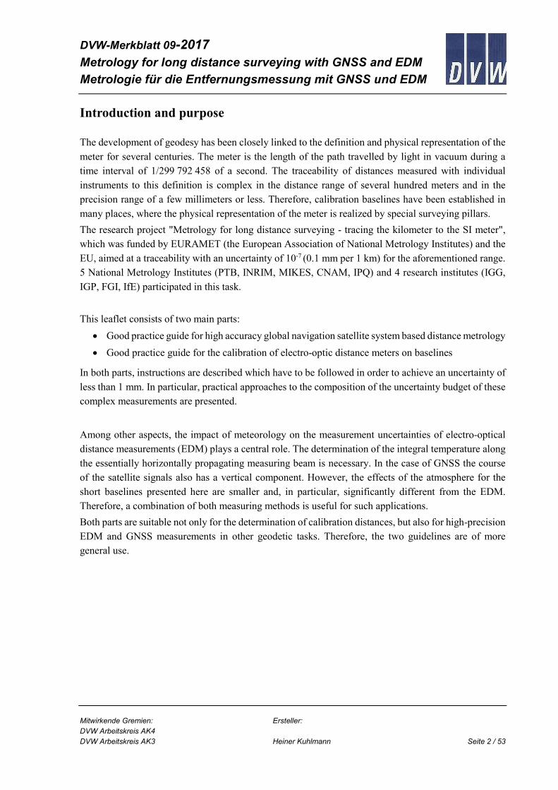
Merkblatt 09-2017
Metrology for long distance surveying with GNSS and EDM
Metrologie für die Entfernungsmessung mit GNSS und EDM
Authors: Milena Astrua (INRIM), Andreas Bauch (PTB), Liliana Eusébio (IPQ),
(in alphabetical order) Thomas Fordell (MIKES), Christa Homann (IGP), Jorma Jokela (FGI),
Ulla Kallio (FGI), Hannu Koivula (FGI), Heiner Kuhlmann (IGG), Sonja
Lahtinen (FGI), Fátima Marques (IPQ), Wolfgang Niemeier (IGP), Olivier
Pellegrino (IPQ), Carlos Pires (IPQ), Florian Pollinger (PTB), Markku
Poutanen(FGI), Fernanda Saraiva (IPQ), Steffen Schön (IfE), Dieter
Tengen (IGP), Jean-Pierre Wallerand (CNAM), Florian Zimmermann
(IGG), Massimo Zucco (INRIM)
Institution of Authors: Physikalisch-Technische Bundesanstalt (PTB), Germany Instituto Português da Qualidade (IPQ), Portugal
Instituto Nazionale di Ricercia Metrologica (INRIM), Italy
VTT Technical Research Centre of Finland Ltd, Centre for Metrology
MIKES, Finland
Conservatoire National des Arts et Métiers (CNAM), France
Finnish Geospatial Research Institute (FGI), Finland
University of Bonn, Institute of Geodesy and Geoinformation (IGG),
Germany
Leibniz Universität Hannover, Institut für Erdmessung (IfE), Germany
Technische Universität Braunschweig, Institut für Geodäsie und
Photogrammetrie (IGP), Germany
Beteiligte Gremien: DVW Arbeitskreis 4, Ingenieurgeodäsie
DVW Arbeitskreis 3, Messmethoden und Systeme
Beschlussfassung: Beschlossen von DVW Arbeitskreis 4 am 03.11.2016
Beschlossen von DVW Arbeitskreis 3 am 08.05.2017
Verabschiedet vom Präsidium des DVW am 08.05.2017
Dokumentenstatus:
verabschiedet
DVW-Merkblatt 09-2017
Metrology for long distance surveying with GNSS and EDM
Metrologie für die Entfernungsmessung mit GNSS und EDM
Mitwirkende Gremien: Ersteller:
DVW Arbeitskreis AK4
DVW Arbeitskreis AK3 Heiner Kuhlmann Seite 2 / 53
Introduction and purpose
The development of geodesy has been closely linked to the definition and physical representation of the
meter for several centuries. The meter is the length of the path travelled by light in vacuum during a
time interval of 1/299 792 458 of a second. The traceability of distances measured with individual
instruments to this definition is complex in the distance range of several hundred meters and in the
precision range of a few millimeters or less. Therefore, calibration baselines have been established in
many places, where the physical representation of the meter is realized by special surveying pillars.
The research project "Metrology for long distance surveying - tracing the kilometer to the SI meter",
which was funded by EURAMET (the European Association of National Metrology Institutes) and the
EU, aimed at a traceability with an uncertainty of 10-7 (0.1 mm per 1 km) for the aforementioned range.
5 National Metrology Institutes (PTB, INRIM, MIKES, CNAM, IPQ) and 4 research institutes (IGG,
IGP, FGI, IfE) participated in this task.
This leaflet consists of two main parts:
• Good practice guide for high accuracy global navigation satellite system based distance metrology
• Good practice guide for the calibration of electro-optic distance meters on baselines
In both parts, instructions are described which have to be followed in order to achieve an uncertainty of
less than 1 mm. In particular, practical approaches to the composition of the uncertainty budget of these
complex measurements are presented.
Among other aspects, the impact of meteorology on the measurement uncertainties of electro-optical
distance measurements (EDM) plays a central role. The determination of the integral temperature along
the essentially horizontally propagating measuring beam is necessary. In the case of GNSS the course
of the satellite signals also has a vertical component. However, the effects of the atmosphere for the
short baselines presented here are smaller and, in particular, significantly different from the EDM.
Therefore, a combination of both measuring methods is useful for such applications.
Both parts are suitable not only for the determination of calibration distances, but also for high-precision
EDM and GNSS measurements in other geodetic tasks. Therefore, the two guidelines are of more
general use.

DVW-Merkblatt 09-2017
Metrology for long distance surveying with GNSS and EDM
Metrologie für die Entfernungsmessung mit GNSS und EDM
Mitwirkende Gremien: Ersteller:
DVW Arbeitskreis AK4
DVW Arbeitskreis AK3 Heiner Kuhlmann Seite 3 / 53
Einordnung und Zweck
Die Entwicklung der Geodäsie ist seit einigen Jahrhunderten eng mit der Definition und physischen
Repräsentation des Meters verknüpft. Die Einheit Meter ist heute klar definiert: Ein Meter ist die
Weglänge, die das Licht im Vakuum in einem Zeitintervall von 1/299 792 458 s zurücklegt. Die
Rückführung der mit einzelnen Messinstrumenten gemessenen Entfernungen auf diese Definition ist im
Entfernungsbereich von einigen hundert Metern und im Genauigkeitsbereich von wenigen Millimetern
und darunter aufwändig. Daher wurden vielerorts mit Vermessungspfeilern vermarkte Kalibrierstrecken
zur physischen Repräsentation des Meters etabliert.
Das von EURAMET (Europaen Association of National Metrology Institutes) und der EU finanzierte
Forschungsprojekt „Metrology for long distance surveying - Tracing the kilometre to the SI metre“ hatte
u.a. zum Ziel, die Rückführbarkeit mit einer Unsicherheit von 10-7 (0,1 mm auf 1 km) für den genannten
Entfernungsbereich zu erreichen. An dieser Aufgabe beteiligten sich fünf nationale Metrologie-Institute
(PTB, INRIM, MIKES, CNAM, IPQ) sowie vier Forschungseinrichtungen (IGG, IGP, FGI, IfE).
Dieses Merkblatt hat zwei Hauptbestandteile:
• Good practice guide for high accuracy global navigation satellite system based distance metrology
• Good practice guide for the calibration of electro-optic distance meters on baselines
In beiden Teilen sind die Maßnahmen geschildert, die zur Erreichung der genannten Messunsicherheit
von weniger als 1 mm einzuhalten sind. Insbesondere wird die Zusammensetzung des
Unsicherheitsbudgets dargestellt.
Neben anderen Aspekten spielt die Auswirkung der Meteorologie auf die Messunsicherheiten der
elektro-optischen Entfernungsmessung (EDM) eine zentrale Rolle; hierbei ist die Bestimmung der
integralen Temperatur des im Wesentlichen horizontal verlaufenden Signalwegs notwendig. GNSS
Signale werden an Empfangsantennen aus unterschiedlichen Richtungen empfangen, so dass die
Auswirkungen der Atmosphäre deutlich verschieden gegenüber der EDM sind. Daher ist eine
Kombination der beiden Messverfahren für die im Folgenden beschriebenen Anwendungen sinnvoll.
Beide Teile eignen sich nicht nur zur Bestimmung von Kalibrierstrecken, sondern können auch
Anhaltspunkte für hochpräzise EDM- und GNSS-Messungen bei anderen geodätischen Aufgaben
geben. Daher sind die beiden Leitlinien von allgemeinerem Nutzen, sie sollten jedoch nicht
ausschließlich berücksichtigt werden, sondern sind in Ergänzung zu einschlägiger Fachliteratur zu
nutzen
SURVEYING Good practice guide
EMRP JRP SIB60 Dissemination level: Public
Mitwirkende Gremien: © SURVEYING JRP-Consortium 2016
DVW Arbeitskreis AK4
DVW Arbeitskreis AK3 Seite 4 / 53
Good practice guide for
high accuracy global navigation satellite system
based distance metrology
Revised Version 2

SURVEYING Good practice guide
EMRP JRP SIB60 Dissemination level: Public
Mitwirkende Gremien: © SURVEYING JRP-Consortium 2016
DVW Arbeitskreis AK4
DVW Arbeitskreis AK3 Seite 5 / 53
Imprint
Authors:
Andreas Bauch1 Liliana Eusébio2
Ulla Kallio3
Hannu Koivula3
Heiner Kuhlmann4
Sonja Lahtinen3
Fátima Marques2
Olivier Pellegrino2
Carlos Pires2
Florian Pollinger1 Markku Poutanen3
Fernanda Saraiva2
Steffen Schön5
Florian Zimmermann4
1Physikalisch-Technische Bundesanstalt (PTB), Bundesallee 100, 38116 Braunschweig, Germany 2Instituto Português da Qualidade (IPQ), Rua Antón io Gião 2, 2829-513 Caparica, Portugal 3Finnish Geospatial Research Institute (FGI), Geodeetinrinne 2, 02430 Masala, Finland 4University of Bonn, Institute of Geodesy and Geoinformation, Nußallee 17, 53115 Bonn, Germany 5Leibniz Universität Hannover, Institut für Erdmessung, Schneiderberg 50, 30167 Hannover, Germany
Contact email: [email protected]
These good practice guidelines were developed in 2016 by the JRP SIB60 “Metrology for Long Distance Surveying”
as part of the European Metrology Research Programme EMRP run by EURAMET e.V. All procedures were developed with best knowledge.
Neither the authors nor EURAMET e.V., however, can be held accountable for any damage caused by the application of these guidelines.
The good practice guide may not be altered or copied as excerpts without written consent of the
author team. The good practice guide as a whole can be freely distributed.
Braunschweig, September 16, 2016 (date of the revised version May 24, 2017)


SURVEYING Good practice guide
EMRP JRP SIB60 Dissemination level: Public
Mitwirkende Gremien: © SURVEYING JRP-Consortium 2016
DVW Arbeitskreis AK4
DVW Arbeitskreis AK3 Seite 7 / 53
Contents
Executive summary .......................................................................................................................................... 8
1 Introduction ............................................................................................................................................. 9
2 Scope and field of application ................................................................................................................ 10
3 Preparation ............................................................................................................................................ 11
3.1 Antenna calibration ............................................................................................................................. 11 3.2 Station set-up ...................................................................................................................................... 11 3.3 Schematic description of the set-up .................................................................................................... 13
4 Measurement strategy .......................................................................................................................... 14
4.1 Recommendation on the actual measurement ................................................................................... 14 4.2 Data format ......................................................................................................................................... 14 4.3 Data processing ................................................................................................................................... 14
5 Assessment of uncertainties of GNSS-distances ..................................................................................... 16
5.1 Introduction ......................................................................................................................................... 16 5.2 Approximation of the combined uncertainty ...................................................................................... 17
References ..................................................................................................................................................... 18
Acknowledgements ........................................................................................................................................ 19

SURVEYING Good practice guide
EMRP JRP SIB60 Dissemination level: Public
Mitwirkende Gremien: © SURVEYING JRP-Consortium 2016
DVW Arbeitskreis AK4
DVW Arbeitskreis AK3 Seite 8 / 53
Executive summary
This guidance document has been written to meet the need for a basic document for laboratories undertaking the use of GNSS based distance meters (GBDM) with accuracies in the millimetre regime using geodetic grade GNSS equipment for antennae, receivers, and software analysis. The focus of this document is the identification, quantification, and recommendations on minimisation of experimental uncertainty sources for the GBDM in surveying practice in this uncertainty regime. The algorithmic data analysis is not within the scope of this document. Conclusions are mainly based on the results of respective experimental studies performed by the joint research project (JRP) “SIB60 metrology for long distance surveying” as part of the European metrology research programme (EMRP) between July 2013 and June 2016, but takes into account state of the art of respective literature.

SURVEYING Good practice guide
EMRP JRP SIB60 Dissemination level: Public
Mitwirkende Gremien: © SURVEYING JRP-Consortium 2016
DVW Arbeitskreis AK4
DVW Arbeitskreis AK3 Seite 9 / 53
1 Introduction
The purpose of this technical guideline is to improve harmonisation and to suggest good practices on the use of GBDM measurements. The guideline is based on the experiments performed by the joint research project “SIB60 metrology for long distance surveying” as part of the European metrology research programme (EMRP) between July 2013 and June 2016.
It is structured in three main chapters: chapter 3 is dealing with preparatory measures on the hardware, including calibration needs of the electromagnetic properties of the antennae and an optimized station set up. Chapter 4 focuses on the actual measurement situation, with a focus on the tropospheric correction strategy. In chapter 5, an exemplary quantitative assessment of uncertainties and their propagation in typical GBDM analysis is given although a full uncertainty budget according to the “Guide to the Expression of Uncertainty (GUM)” cannot be provided because several influence factors are known but without a firm mathematical relation that would allow the error propagation to be calculated unambiguously.

SURVEYING Good practice guide
EMRP JRP SIB60 Dissemination level: Public
Mitwirkende Gremien: © SURVEYING JRP-Consortium 2016
DVW Arbeitskreis AK4
DVW Arbeitskreis AK3 Seite 10 / 53
2 Scope and field of application
This guideline refers to distance measurements of several hundred metres up to a few kilometres performed with geodetic grade GNSS equipment for antennae, receivers, and software analysis with targeted uncertainties between several tenths of millimetres up to millimetres based on relative positioning.
The guideline provides recommendations for optimized strategies for set-up and analysis procedures, taking into account the leading uncertainty sources at this uncertainty level. These are the characterization of the electromagnetic antenna properties, near-field and multipath effects and environmental corrections.
The guideline does not cover proper general handling of the equipment or particularities of different analysis strategies or standard software packages.
An exemplary treatment of uncertainty propagation is included. However, the quantitative applicability of this example depends strongly on the actual measurement situation on site. This study does not allow conclusions on the general performance of specific software packages.
SURVEYING Good practice guide
EMRP JRP SIB60 Dissemination level: Public
Mitwirkende Gremien: © SURVEYING JRP-Consortium 2016
DVW Arbeitskreis AK4
DVW Arbeitskreis AK3 Seite 11 / 53
3 Preparation
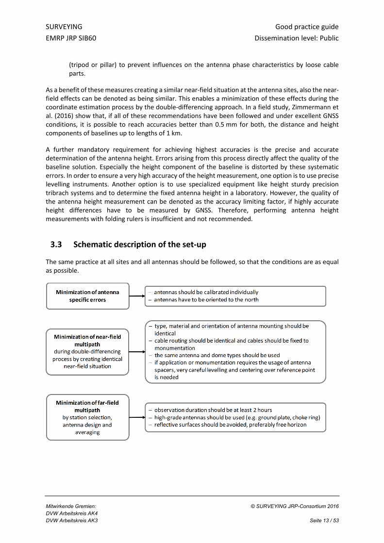
In high-precision GNSS applications, usually a relative position estimation using carrier-phase measurements is performed. By forming double-differences of the observables, the majority of systematic errors, e.g. satellite orbit and clock errors, atmospheric delays or receiver clock errors, can be completely eliminated or at least minimized. One of the remaining accuracy limiting factors are station dependent errors, e.g. multipath or antenna errors. They cannot be prevented or eliminated by standard processing strategies, since they depend on the antenna surrounding, the antenna set-up, and the antenna. In order to reduce the influences of these error sources, the station set-up has to be optimized. This optimization includes the usage of individually calibrated antennas and an identical station set-up of the antenna stations included in the position and distance estimation process.
3.1 Antenna calibration
In a coordinate estimation process, the observations are assumed to refer to one fixed point, the so called antenna reference point (ARP). In reality, the position of the reference point for the carrier-phase observations depends on the direction of the incoming signal (azimuth α, elevation β). The overall frequency-dependent impact can be described by two components: (1) the phase centre offset (PCO), denoting the position of the mean phase centre in relation to the antenna reference point, and (2) the phase centre variations (PCV), denoting the direction-dependent variations of the mean phase centre.
In recent years, two procedures were proven to be the most effective approaches to calibrate GNSS antennas: absolute robot calibration and a calibration in an anechoic chamber (Wübbena et al., 2000; Zeimetz and Kuhlmann, 2008). Since antennas of the same type show similar phase centre characteristics, type specific calibrations (type mean), e.g. provided by the IGS (ftp://igscb.jpl.nasa.gov/igscb/station/general/igs08.atx), can be used to reduce the influences described above. Nevertheless, an optimum elimination of the influences can only be achieved by using individually calibrated antennas. The differences between individual calibrations and type mean calibrations can reach several millimetres. Especially for the PCO values, this is critical, since deviations in this parameter will lead to systematic errors in the estimated coordinates. Thus, for GNSS applications with very high accuracy requirements at the millimetre or sub-millimetre level, it is strongly recommended to use individually absolute calibrated antennas. A concise introduction into antenna calibration and correction parameters can be found in DVW Merkblatt 1 (Zeimetz et al., 2011).
3.2 Station set-up
In addition to antenna specific errors, GNSS multipath is a further site dependent error which has to be taken into account. In general, multipath can be separated into far-field and near-field multipath (Wübbena et al., 2006). Far-field effects arise from reflecting surfaces in the environment of the antenna and lead to one or more signals arriving at the antenna by indirect paths (Hofmann-Wellenhof et al., 2008). The interference of the direct and indirect signals leads to short periodic errors in the observation and position domain, which can be averaged out by sufficiently long observation times (Seeber, 2003). Furthermore, far-field multipath can be reduced by a special antenna design, e.g. antennas with ground plates or choke rings. Nevertheless, it is recommended to carefully select the observation site. Reflecting surfaces in the environment of the antenna, especially vertical surfaces

SURVEYING Good practice guide
EMRP JRP SIB60 Dissemination level: Public
Mitwirkende Gremien: © SURVEYING JRP-Consortium 2016
DVW Arbeitskreis AK4
DVW Arbeitskreis AK3 Seite 12 / 53
leading reflections from above the antenna horizon should be avoided and a preferably free horizon should be targeted.
In contrast, near-field multipath results from the closest vicinity of the antenna, often described as the first 50 cm around the antenna. On one hand, near-field effects can lead to long-periodic errors, which result in a non-zero mean distributed and un-modelled bias in the estimated parameters. On the other hand, the antenna near-field can change the overall electromagnetic properties of the antenna (Dilssner, 2008). Hence, individual antenna calibrations, as described in section 3.1, are actually only valid if the near-field situation has also been reproduced during the calibration procedure (Wübbena, 2006). Nevertheless, size and weight limitations usually preclude this kind of near-field calibration.
One attempt to reduce influences from the first 50 cm around the antenna might be to use antenna spacers to increase the distance between the antenna mounting and the antenna itself. This approach, however, has three disadvantages:
• If the antenna spacer exceeds lengths of 40 cm to 50 cm, the whole set-up becomes unstable. Especially for heavy antennas, e.g., choke-ring antennas, this is critical. Thus, in case of very long spacers, additional effort is necessary to stabilize the set-up.
• The exact straightness of the antenna spacers has to be ensured, since a bending of the spacer can lead to a systematic error in the estimated baseline lengths, which is proportional to the spacer length. Moreover, the centre of the bottom thread and the screw on top of the spacer have to coincide precisely, e.g. below the required sub mm accuracy level. Deviations between these two points will also lead to systematic errors of the same magnitude. As a consequence, the accuracy requirements during the manufacturing of the antenna spacers are extremely high.
• To reach a very high accuracy level, the antenna spacers have to be levelled and centred accurately over the reference point of the antenna monument station. Since this is the most crucial step during the whole measurement process, a lot of effort and precise measurement equipment is required.
Due to these disadvantages, it is not recommended to use antenna spacers to reduce the influence of the antenna near-field. Hence, only if the application or the antenna site requires the usage of additional spacers between the antenna and the antenna mount, spacers should be used.
Since near-field effects arise from the closest vicinity of the antenna, for applications in which distance determination with highest accuracy is required, it is recommended to create a preferably identical near-field situation at all antenna sites.
• The same antenna types should be used at all stations. Since the antenna calibration patterns described in section 3.1 are direction dependent, the antennas have to be oriented to the north to utilize the full potential of the antenna corrections.
• Furthermore, the type and material of the antenna mounting, like e.g., tribrach, tripod, pillar, etc., as well as the orientation of the respective parts, should be identical.
• In addition, it is well known that the routing of the antenna cable can have a direct impact on the phase centre characteristic of the antenna (Zeimetz and Kuhlmann, 2008). Thus, also the cable routing should be identical and the antenna cables should be fixed to the antenna mount
SURVEYING Good practice guide
EMRP JRP SIB60 Dissemination level: Public
Mitwirkende Gremien: © SURVEYING JRP-Consortium 2016
DVW Arbeitskreis AK4
DVW Arbeitskreis AK3 Seite 13 / 53
(tripod or pillar) to prevent influences on the antenna phase characteristics by loose cable parts.
As a benefit of these measures creating a similar near-field situation at the antenna sites, also the near-field effects can be denoted as being similar. This enables a minimization of these effects during the coordinate estimation process by the double-differencing approach. In a field study, Zimmermann et al. (2016) show that, if all of these recommendations have been followed and under excellent GNSS conditions, it is possible to reach accuracies better than 0.5 mm for both, the distance and height components of baselines up to lengths of 1 km.
A further mandatory requirement for achieving highest accuracies is the precise and accurate determination of the antenna height. Errors arising from this process directly affect the quality of the baseline solution. Especially the height component of the baseline is distorted by these systematic errors. In order to ensure a very high accuracy of the height measurement, one option is to use precise levelling instruments. Another option is to use specialized equipment like height sturdy precision tribrach systems and to determine the fixed antenna height in a laboratory. However, the quality of the antenna height measurement can be denoted as the accuracy limiting factor, if highly accurate height differences have to be measured by GNSS. Therefore, performing antenna height measurements with folding rulers is insufficient and not recommended.
3.3 Schematic description of the set-up
The same practice at all sites and all antennas should be followed, so that the conditions are as equal as possible.

SURVEYING Good practice guide
EMRP JRP SIB60 Dissemination level: Public
Mitwirkende Gremien: © SURVEYING JRP-Consortium 2016
DVW Arbeitskreis AK4
DVW Arbeitskreis AK3 Seite 14 / 53
4 Measurement strategy
Aside from a sensible station set-up, the choice of the measurement strategy is of utmost importance for the achievable accuracy of GNSS-based distance measurements. In the following, recommendations for the actual measurement, but also data format and data processing are given.
4.1 Recommendations on the actual measurement
The following two issues are basic prerequisites for high accuracy GNSS-based distance measurements:
• Measurements have to be performed under valid meteorological conditions, in the temperature ranges stated by the manufacturer.
• As mentioned already in section 3.3, an observation time of at least 2 hours should be kept.
4.2 Data format
The receiver internal algorithms are proprietary, so it is difficult to assess the influence on the "raw observations" that the respective data processing for geodetic applications is using. Studying software receivers could help to some extend to identify in laborious experiments the impact of different firmware versions of GNSS receivers. Consequently, data in the Receiver Independent Exchange Format RINEX is considered as raw data. However, experience shows that also the convertor from raw data to RINEX may impact the data. Finally from a physical point, short delay multipath (< 0.1 µs or 30 m) is the most critical since it is very hard to separate it from the direct signal. The analysis of the - hopefully soon available and stable/final - Galileo signals with new modulation schemes may help to push this part.
4.3 Data processing
Different data processing schemes are possible in GNSS analysis. They may differ in the observables used, the weighting of observations, and the estimation of additional parameters, like the tropospheric zenith delays. Different processing schemes may yield to differences in the estimated coordinates of up to a few centimetres.
In Beutler et al. (1989), Santerre (1991), and Rothacher (2002) the correlations between the geodetic parameters height, troposphere and receiver clock are explained. Rules of thumb are given how remaining systematic effects affect the estimated coordinates. Applications to small networks are presented in Rothacher (2000), while the impact with large height differences is discussed in Schön (2007). Examples for violations of the similarity hypothesis between the endpoints of GNSS baselines are discussed in Schön (2010). Brockmann et al. (2010) discusse the impact of different processing strategies on co-located stations in the Swiss AGNES network, where ground truth information from local ties is available, measured by terrestrial instruments. In addition, Schön et al. (2016) proposed an easy-to-use post-processing strategy to remove discrepancies between local ties and GNSS-derived heights when tropospheric effects are mis-modeled.
For short baselines (few meters to up to 1-2 km) we recommend to
SURVEYING Good practice guide
EMRP JRP SIB60 Dissemination level: Public
Mitwirkende Gremien: © SURVEYING JRP-Consortium 2016
DVW Arbeitskreis AK4
DVW Arbeitskreis AK3 Seite 15 / 53
• Use the most precise L1 carrier phase observations: The noise in the observation is minimized as well as that of the estimated coordinates.
• Form double-differences: Double-differences combine four GNSS carrier phase observations into one new observable. As argued in chapter 3 with respect to the station set up, this analysis concept that reduces largely systematic effects that are similar at both stations and at both satellites as well as along the signal propagation path. Subsequently, as long as the similarity is preserved by identical equipment, dedicated site selection, and similar atmospheric conditions (e.g. only small height differences), most of the systematic effects can be largely reduced or even eliminated.
• The role of ionosphere modelling can be assumed negligible.
• In case of tropospheric zenith path delay parameters are estimated, two cases need to be
distinguished:
1. If stations are at same height, do not estimate tropospheric zenith path delay parameters. For short station distances, and negligible station height differences, physical tropospheric delay do not persist in double-difference analysis. If troposphere parameters are modelled in such a set up, the impact of non-modelled systematic effects will be increased by estimating tropospheric zenith path delays. The adjustment model is changed due to the large correlation between height, troposphere parameters, and receiver clocks. This deteriorates the coordinate solution, especially the height by up to some millimetres (Krawinkel et al., 2014).
2. If substantial height differences between the stations exist or the station separation exceeds a few hundred meters , asymmetries are generated which cannot be eliminated by forming differences. Then tropospheric delay parameters have to be estimated with respect to the duration of the observation (e.g., one parameter per 30 minutes). This estimation weakens the geometry of the adjustment problem and introduces in relative positioning correlations between height and tropospheric delay.
SURVEYING Good practice guide
EMRP JRP SIB60 Dissemination level: Public
Mitwirkende Gremien: © SURVEYING JRP-Consortium 2016
DVW Arbeitskreis AK4
DVW Arbeitskreis AK3 Seite 16 / 53
5 Assessment of uncertainties of GNSS-distances
GNSS based distance measurements are often used for official, e.g. cadastral, work or in case of long-term monitoring implying the need of long-term comparability and indepedence from operator, method and equipment. This requires stringent traceability to the SI definition of the metre and a systematic and standardized assessment of the measurement uncertainty associated with the measured quantity. The various external input parameters into the analysis of a GNSS based distance measurement, however, prevent a stringent uncertainty analysis of a distance measurement performed by GNSS. In the following sections an approximative assessment of the achievable uncertainty is proposed.
5.1 Introduction: uncertainty and GNSS based distance measurement
Although the distance information is derived in ultimo from atomic clock signals, traceabiliy to the SI definition of the metre of a GNSS-based distance measurement severely suffers from the following issues:
• The user has little information neither on the uncertainties of the provided satellite orbit data, nor in the propagation of these uncertainties when using standard software packages.
• Propagation of the signal through the ionosphere and troposphere, effect of multipath, antenna phase center variations and other sources of error are not controllable and are mostly unknown during the data processing.
Although one can estimate the magnitude of these variables in the analysis, uncertainties of these estimations are mostly unknown, and especially their propagation into the final results. As a consequence, analyses of the same data using different software applying their recommended set of parameters will produce different results and uncertainties.
One way to assess the uncertainty of the GNSS-distances on a given site for the specific local situation and equipment used is a direct comparison of GNSS-based distance measurements compared to reference distances measured with a calibrated instrument with the scale traceable to the SI definition of the meter. The sensitivity of the GNSS-based distance measurement to the local surrounding (multipath effects) infers that the results of such comparisons should not be applied to other measurement configurations without further considerations.
In the course of the European joint research project “Metrology for long distance surveying” the Monte Carlo Method (MCM) was used for an assessment of the sensitivity of GNSS coordinate differences and distances on small changes in antenna calibration table, troposphere correction difference and multipath. Although MCM can be improved by developing the models of uncertainty sources, the accuracy of the method is limited by the number of the MCM iteration rounds. In each interaction a new full set of GNSS observation data are generated which must be processed by the GNSS software. This is not applicable in practice for routine uncertainty estimation.
In daily practice, the surveyor can get a realistic uncertainty estimate using empirical data and a traceable reference distance on site. The assessment of the combined uncertainty of GNSS measurements based on reference measurements are summarized in the next section.

SURVEYING Good practice guide
EMRP JRP SIB60 Dissemination level: Public
Mitwirkende Gremien: © SURVEYING JRP-Consortium 2016
DVW Arbeitskreis AK4
DVW Arbeitskreis AK3 Seite 17 / 53
5.2 Approximation of the combined uncertainty
The combined uncertainty of the GNSS lengths can be computed based on the standard deviation of the GNSS length, the EDM reference measurement and its uncertainty:
( ) ( ) ( )22 2
GPS GPS-EDM ref comp( )u l l u l u l≈ ∆ + + (1)
where
GPS-EDMl∆ deviation of the GNSS from the EDM distance as an estimate of the magnitude of
systematic effects like multipath, obstruction and so on, acquired under similar environmental and local conditions as the actual measurement
( )refu l standard uncertainty of the independent SI traceable reference measurement, and
( )compu l computed standard deviation of the GNSS length
The standard deviations of the GNSS lengths ( )compu l are derived from the standard deviations of the
coordinates reported in the final results of the GNSS processing. It includes only one part of the uncertainty sources. The other part can be estimated by the difference between the GNSS and a SI-
traceable reference (e.g. EDM or total station) lengths GPS-EDMl∆ and by the uncertainties ( )refu l of
these reference measurements themselves.
As an example, the analysis was applied to daily GNSS solutions at baselines monitored in Finland in the Surveying project. There, the estimated combined uncertainties according to equation (1) varied between 0.1 and 0.9 mm. The magnitude did not depend on the baseline length. It should be noted
that the standard deviations for the GNSS lengths ( )compu l were in all cases below 0.05 mm. The
uncertainties of the reference distances ( )EDMu l were below 0.1 mm for lengths shorter than 100 m
and below 0.2 mm for the longest baselines (< 200 m). Hence, the observed differences to the EDM based reference distance GPS-EDMl∆ were the most dominating factor of the combined uncertainty. This
quantity indicates the magnitude of uncertainty contributions which would otherwise require complex and intricate advanced modelling.

SURVEYING Good practice guide
EMRP JRP SIB60 Dissemination level: Public
Mitwirkende Gremien: © SURVEYING JRP-Consortium 2016
DVW Arbeitskreis AK4
DVW Arbeitskreis AK3 Seite 18 / 53
References
Beutler, G.; Bauersima, I.; Botton, S.; Gurtner, W.; Rothacher, M.; Schildknecht, T. (1989). Accuracy and biases in the geodetic application of the Global Positioning System. Manuscripta Geodaetica 14, pp. 28-35.
Brockmann, E.; Ineichen, D.; Schär, S.; Schlatter, A. (2010). Use of double stations in the Swiss Permanent GNSS Network AGNES. Proceeding EUREF 2010, 6p.
Dilssner, F.; Seeber, G.; Wübbena, G.; Schmitz, M. (2008). Impact of near-field effects on the GNSS position solution. In: Proceedings of the 21st International Technical Meeting of the Satellite Division of The Institute of Navigation (ION GNSS 2008), 2008, pp. 612–624.
Hofmann-Wellenhof, B.; Lichtenegger, H.; Wasle, E. (2008). GNSS-Global Navigation Satellite Systems: GPS, GLONASS, Galileo & more, Springer, Wien.
Krawinkel, T.; Lindenthal, N.; Schön, S. (2014). Scheinbare Koordinatenänderungen von GPS-Referenzstationen: Einfluss von Auswertestrategien und Antennenwechseln, ZfV 139, pp. 252-263.
Rothacher, M. (2000). Hochgenaue regionale und kleinräumige GPS-Netze: Fehlerquellen und Auswertestrategien. Mitteilungsblatt DVW-Bayern 52(2), pp. 153-172, Deutscher Verein für Vermessungswesen, Landesverband Bayern, ISSN 0723-6336.
Rothacher, M. (2002). Estimation of station heights with GPS. In: Drewes, H.; Dodson, A.; Fortes, L.P.S.; Sánchez, L.; Sandoval, P. (eds.) Vertical Reference Systems, IAG Symposia, Vol. 124, pp 81-90, Springer, ISBN (Print) 978-3-540-43011-7.
Santerre, R. (1991). Impact of GPS satellite sky distribution. Manuscripta geodaetica 16, pp. 28-53.
Seeber, G. (2003). Satellite Geodesy, 2nd edn, Walter deGruyter, Berlin.
Schön, S. (2007). Affine distortion of small GPS networks with large height differences. GPS Sol 11, pp. 107-117.
Schön, S. (2010). Differentielle GNSS Systeme - Code und Phasenlösungen. In: Scheider A, Schwieger V: GNSS2010 - Vermessung und Navigation im 21 Jahrhundert DVW Schriftenreihe 63, pp. 15-38.
Schön, S.; Pham, K.; Krawinkel, T. (2016). On Removing Discrepancies Between Local Ties and GPS-based Coordinates. In IAG Symposia IUGG Prague, accepted, DOI:10.1007/1345_2016_238.
Wübbena, G.; Schmitz, M.; Menge, F.; Böder, V.; Seeber, G. (2000). Automated Absolute Field Calibration of GPS Antennas in Real-Time. In: Proceedings of the 13th International Technical Meeting of the Satellite Division of The Institute of Navigation (ION GPS 2000), Salt Lake City, UT, September 19-22, 2000, pp. 2512–2522.
Wübbena, G.; Schmitz, M.; Boettcher, G. (2006). Near-field effects on GNSS sites: analysis using absolute robot calibrations and procedures to determine corrections. In: Proceedings of the IGS Workshop 2006 Perspectives and Visions for 2010 and beyond, Darmstadt, Germany, May 8-12. 2006, pp. 8–12.
Zeimetz, P.; Becker, M.; Kuhlmann, H.; Schön, S.; Wanninger, L. (2011) Berücksichtigung von Antennenkorrekturen bei GNSS-Anwendungen. DVW Merkblatt 1. Available online under http://www.dvw.de/merkblatt.
Zeimetz, P.; Kuhlmann, H. (2008). On the accuracy of absolute GNSS antenna calibration and the conception of a new anechoic chamber. In: Proceedings of the FIG Working Week 2008, Stockholm, Sweden, June 14-19.
Zimmermann, F.; Eling, C.; Kuhlmann, H. (2016); Investigations on the influence of Antenna Near-Field Effects and Satellite Obstruction on the Uncertainty of GNSS-based Distance Measurements. Journal of Applied Geodesy, 10 (1), ahead of print.

SURVEYING Good practice guide
EMRP JRP SIB60 Dissemination level: Public
Mitwirkende Gremien: © SURVEYING JRP-Consortium 2016
DVW Arbeitskreis AK4
DVW Arbeitskreis AK3 Seite 19 / 53
Acknowledgements
We gratefully acknowledge funding from the European Metrology Research Program (EMRP). The EMRP is jointly funded by the EMRP participating countries within EURAMET and the European Union.
SURVEYING Good practice guide
EMRP JRP SIB60 Dissemination level: Public
Mitwirkende Gremien: © SURVEYING JRP-Consortium 2016
DVW Arbeitskreis AK4
DVW Arbeitskreis AK3 Seite 20 / 53
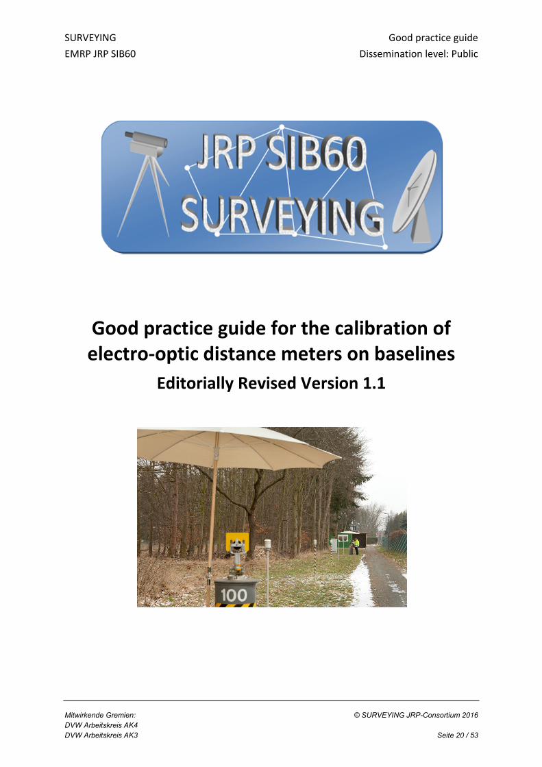
Good practice guide for the calibration of
electro-optic distance meters on baselines
Editorially Revised Version 1.1

SURVEYING Good practice guide
EMRP JRP SIB60 Dissemination level: Public
Mitwirkende Gremien: © SURVEYING JRP-Consortium 2016
DVW Arbeitskreis AK4
DVW Arbeitskreis AK3 Seite 21 / 53
Imprint
Authors:
Milena Astrua1
Thomas Fordell2 Christa Homann3
Jorma Jokela4 Wolfgang Niemeier3 Florian Pollinger5
Dieter Tengen3
Jean-Pierre Wallerand6 Massimo Zucco1
1Instituto Nazionale di Ricercia Metrologica (INRIM), Strada delle Cacce 91, 10135 Torino, Italy 2VTT Technical Research Centre of Finland Ltd, Centre for Metrology MIKES, P.O. Box 1000, FI-02044 VTT, Finland 3Technische Universität Braunschweig, Institut für Geodäsie und Photogrammetrie, Pockelsstraße 3, 38106 Braunschweig, Germany 4Finnish Geospatial Research Institute (FGI), Geodeetinrinne 2, 02430 Masala, Finland 5Physikalisch-Technische Bundesanstalt (PTB), Bundesallee 100, 38116 Braunschweig, Germany 6Conservatoire National des Arts et Métiers (CNAM), 292 rue Saint-Martin, 75141 Paris Cédex 03, France
Contact email: [email protected]
These good practice guidelines were developed in 2016 by the JRP SIB60 “Metrology for Long Distance Surveying”
as part of the European Metrology Research Programme EMRP run by EURAMET e.V. All procedures were developed with best knowledge.
Neither the authors nor EURAMET e.V., however, can be held accountable for any damage caused by the application of these guidelines.
The good practice guide may not be altered or copied as excerpts without written consent of the
author team. The good practice guide as a whole can be freely distributed.
Braunschweig, September 16, 2016 (date of the editorially revised version May 24, 2017)


SURVEYING Good practice guide
EMRP JRP SIB60 Dissemination level: Public
Mitwirkende Gremien: © SURVEYING JRP-Consortium 2016
DVW Arbeitskreis AK4
DVW Arbeitskreis AK3 Seite 23 / 53
Contents
Objectives ...................................................................................................................................................... 24
1 SI traceability and concept of measurement uncertainty ............................................................................ 25
2 Requirements for reference baselines ......................................................................................................... 26
2.1 Location ...................................................................................................................................... 26
2.2 Construction of pillars .................................................................................................................. 26
2.3 Meteorological sensor network ................................................................................................... 27
3 Recommendations for Calibration Measurements ...................................................................................... 28
3.1 Field book .................................................................................................................................... 28
3.2 Synchronisation ........................................................................................................................... 28
3.3 Meteorological compensation ..................................................................................................... 28
3.4 Mounting of the EDM and the reflector ....................................................................................... 28
3.5 Distance observations .................................................................................................................. 29
4 Data Processing ........................................................................................................................................... 30
4.1 General considerations on the processing strategy ....................................................................... 30
4.2 Components of a suitable 3D adjustment model .......................................................................... 31
5 Measurement uncertainty ........................................................................................................................... 35
5.1 Survey on contributions ............................................................................................................... 35
5.2 Influence of the refractive index .................................................................................................. 35
5.3 Influence of turbulence ................................................................................................................ 37
5.4 Projection of the reference point ................................................................................................. 38
5.5 Uncertainty estimate of the calibration parameters ..................................................................... 39
6 Presentation of results ................................................................................................................................ 43
7 Appendix ..................................................................................................................................................... 45
7.1 Field book .................................................................................................................................... 45
7.2 On traceability ............................................................................................................................. 47
8 Literature .................................................................................................................................................... 50
Acknowledgements ........................................................................................................................................ 52
SURVEYING Good practice guide
EMRP JRP SIB60 Dissemination level: Public
Mitwirkende Gremien: © SURVEYING JRP-Consortium 2016
DVW Arbeitskreis AK4
DVW Arbeitskreis AK3 Seite 24 / 53
Objectives
The aim of this guideline is to provide a calibration strategy and a practical solution for surveyors and survey authorities who intend to or by law/regulations have to verify or calibrate their electro-optic distance meters (EDM) on a reference baseline. The content of this document is based on existing literature in the field, many years of practical experience of the authors in EDM calibration and on results of research performed by the joint research project (JRP) “SIB60 metrology for long distance surveying” as part of the European metrology research programme (EMRP) between July 2013 and June 2016
In this report the basic problem of traceability is discussed first to allow the surveyor to evaluate the standard of his calibration procedure with respect to the quality of the applied reference length information.
The specific objective of calibration measurements is typically to estimate the following calibration parameters:
• Scale factor
• Additional constant
For this task, a quality assessment of the used reference baseline is required and specific procedures for carrying out the observations, the data processing and their analysis are given here. As a result estimates for the calibration parameters “scale” and “additional constant” and the associated uncertainty are achieved.
The origin and magnitude of many uncertainty contributions are introduced, as well as a Monte Carlo based approach for the combination of adjustment-based coordinate analysis with uncertainty propagation.
Some information on alternative optical standards for realisation of SI units and the possibility of frequency calibration complete these guidelines.

SURVEYING Good practice guide
EMRP JRP SIB60 Dissemination level: Public
Mitwirkende Gremien: © SURVEYING JRP-Consortium 2016
DVW Arbeitskreis AK4
DVW Arbeitskreis AK3 Seite 25 / 53
1 SI traceability and concept of measurement uncertainty
Length measurements in surveying produce data that is stored and processed often for decades. They are the basis for cadastral archives or risk assessments. It is of utmost importance that the data taken by different instruments and observers is comparable, with a common scale and a common labelling of quality. According to the metre convention, all length measurements should be traceable to the SI definition of the metre:
“The metre is the length of the path travelled by light in vacuum during a time interval of
1/299 792 458 of a second.” (CGPM 1983, Resolution 1)
A calibration measurement must hence make sure that traceability to this definition is secured. The realisation of this definition and traceability of a particular device thereto can never be perfect. The standardized quantitative measure for the quality of a measurand with respect to its agreement with the SI definition is the measurement uncertainty according to the “Guide to the expression of uncertainty in measurement” (ISO/IEC Guide 98-3:2008).
“A measurement result is generally expressed as a single measured quantity value and a
measurement uncertainty.” (ISO 17123-1:2010)
In case of EDM baseline calibrations, one important source of uncertainty is the fact that these measurements are not performed in vacuum but in air. The propagation speed of light depends on the medium. In case of air, models allow the derivation of the index of refraction from the measurement of thermodynamic properties like temperature, ambient pressure, humidity and carbon dioxide contents.
There are different approaches to establish SI traceability of geodetic baselines. One important perquisite for SI traceability is the correct estimate of the associated measurement uncertainty. In the appendix, two different examples for the realisation of traceability to the SI definition of the metre with low uncertainty are given.

SURVEYING Good practice guide
EMRP JRP SIB60 Dissemination level: Public
Mitwirkende Gremien: © SURVEYING JRP-Consortium 2016
DVW Arbeitskreis AK4
DVW Arbeitskreis AK3 Seite 26 / 53
2 Requirements for reference baselines
Following the discussion in section 1 on traceability, establishing a direct link to the SI definition with low measurement uncertainty is a laborious procedure and can only be made for selected so-called reference baselines. For setting up of a reference baseline that will serve calibration measurements for decades, some general requirements can be defined:
2.1 Location
For a reference baseline the location has to be selected carefully.
• A stable geological area with homogeneous soil is required in order to guarantee long-term stability of pillars.
• A shaded location with smooth winds results in low turbulence. If the reference baseline has to serve GNSS measurements as well, a free sky is required.
• Effects due to human activity in the surrounding, e.g. machinery in buildings or traffic loads, have to be avoided.
• To avoid reduction problems to common coordinate systems, the reference baseline should be almost horizontal. To guarantee a good intervisibility between pillars, a slight vertical gradient can help.
• Regarding the length of the baseline, it should be related to the typical distances measured in practical surveying work. In general, the length of the reference baseline is in the range between 500 and 1000 m. A longer baseline is favourable for the determination of the scale factor with low uncertainty.
2.2 Construction of pillars
Regarding the purpose of the reference baselines, high effort is required for the set-up of all the pillars:
• The centering system should guarantee an uncertainty of 0.1 mm and it has to serve for EDM equipment from different manufacturers.
• Required is an identical instrument and target height or very precise information of tribrach zero points.
• Typically six to eight pillars should be used and distributed so that all distances between a minimum and a maximum distance can be realised
For the construction of pillars, refer to DVW Merkblatt 8 (2014) where some specific requirements are given for the optimum construction principles and related problems.
A regular check of the stability of all pillars is mandatory, even if geological and soil conditions are good. This stability check has to be performed with an instrument whose measurement uncertainty should be considerably smaller than the suspected changes of pillar positions. The history of possible displacements of each pillar should be documented.
SURVEYING Good practice guide
EMRP JRP SIB60 Dissemination level: Public
Mitwirkende Gremien: © SURVEYING JRP-Consortium 2016
DVW Arbeitskreis AK4
DVW Arbeitskreis AK3 Seite 27 / 53
It should be mentioned that in principle, it is possible to design the baseline so that the measurement scale (“unit length”) of a specific device under test is sampled systematically (ISO17123-4:2012, Rüeger 1996). Thus, the baseline verification is supposed to be sensitive to cyclic or short periodic errors as well. However, it is challenging to design baselines incorporating the various unit lengths of all devices on the market. More importantly, the typically small cyclic errors of modern instruments are much more reliably detectable by laboratory experiments. Therefore, it is advisable to use a reference system with considerably higher resolution e.g. an interference comparator, for this purpose. In case of a cyclic error, a typical sinusoidal deviation can be identified. This information can either be used to derive a correction formula. Alternatively the amplitude can also be used as an estimate of the magnitude of the uncertainty of this effect, assuming a rectangular probability distribution function.
2.3 Meteorological sensor network
To achieve a high accuracy for the estimation of the calibration parameters (scale factor and additional constant), the knowledge of the atmospheric conditions along the signal path is very important: an uncertainty of 1 °C on the average temperature along the optical path implies that a scale factor lower than 1 mm/km cannot be determined. For this reason a dense sensor field is desirable for a reference baseline, where air temperature, air pressure and relative humidity along the reference baseline are observed parallel to the calibration campaign. All sensors should be mounted in a housing so that they are not directly exposed to solar radiation, but with little thermal contact to their housing. In case of temperature, ventilation of the housing of the temperature sensor is favourable (Eschelbach, 2009). A minimum requirement is the measurement of the temperature at two points, the device and target pillar.
The measurement of the environmental conditions should be frequently performed and recorded with a time stamp. Ideally, the data should be stored automatically. A reading at the beginning and at the end of a single pillar-pillar observation allows interpolation and the assignment of a temperature to one observation. For automatic reading, the thermal inertia of the sensors sets the sensible limit for temporal resolution. An interval of 30 s should provide sufficient resolution for typical scenarios.
It is furthermore advantageous to monitor irradiance in parallel. This quantity monitors the solar power transferred into the environment and is a suitable parameter to characterise homogeneity.
SURVEYING Good practice guide
EMRP JRP SIB60 Dissemination level: Public
Mitwirkende Gremien: © SURVEYING JRP-Consortium 2016
DVW Arbeitskreis AK4
DVW Arbeitskreis AK3 Seite 28 / 53
3 Recommendations for Calibration Measurements
In regular intervals or due to legal prerequisites the responsible surveyor has to perform calibration or verification measurements, for example because she or he has to prove that the used equipment is in agreement with the specifications. It is recommended that these calibration measurements take place at least every year, since the validity of calibration parameters is restricted due to instrumental effects, like aging of electronic sensors, dynamic loads, and extreme weather conditions.. The history of calibration parameters for each instrument should be documented to monitor long-term aging effects and to identify sudden jumps as indicators for instrumental problems.
3.1 Field book
The field book to be used should contain all information on instruments used and their distribution as well as time stamps for every observation. An example for such a field book is given in the appendix.
3.2 Synchronisation
The operators must ensure that all clocks of the sensor network, of the operators and of the EDM under test are synchronized to enable secure assignment and post-processing of the various datasets. The accuracy of the synchronisation should be well below the refreshment interval of the environmental data.
3.3 Meteorological compensation
The correct application of velocity corrections, i.e. the compensation of the index of refraction is of high importance for a successful high accuracy calibration. The environmental sensor data can be entered into most contemporary EDMs and the internal velocity correction is immediately applied by software. In practice, however, this manual procedure is error-prone, provoking typos and extending the actual measurement significantly. Thus, it has turned out that it is more constructive to record the environmental data as described in section 2 and to apply the velocity correction only in the analysis of the whole dataset (in the office). To make this possible, it is important not to adopt any settings for temperature, air pressure and relative humidity within the instrument. It is recommended to use the settings for the standard atmosphere of each instrument instead. In this case, the scale for the internal meteorological correction should be “0 ppm”.
3.4 Mounting of the EDM and the reflector
For each instrument it is necessary to use the same prism that is used in daily operation. The prism constant given by the manufacturer of the prism has to be introduced into the instrument and recorded in the field book. It is expected that the prism constant is applied to the distances.
SURVEYING Good practice guide
EMRP JRP SIB60 Dissemination level: Public
Mitwirkende Gremien: © SURVEYING JRP-Consortium 2016
DVW Arbeitskreis AK4
DVW Arbeitskreis AK3 Seite 29 / 53
The forced centring of the instrument/prism is critical for high accuracy calibration measurements. Even in high quality grade tripods, eccentricities can amount up to several tenths of millimetres. If possible, the tribrachs should remain on the pillars during the whole calibration campaign. Thus, the position of the instrument/prism with respect to the reference point is always the same. If this is not possible, measures like the use of markers should be taken to ensure that the tribrachs have the same rotational position for each calibration.
All tribrachs should be carefully levelled. Suitable instruments are geodetic laser plummets with two perpendicular tubular levels and typical uncertainties in the order of 30 arcseconds.
Instrument and prism heights have to be measured and recorded. The difference should not exceed 15 mm, otherwise the prism carrier is unsuitable for the calibration (see also the respective uncertainty estimate in section 0). To secure constant height offsets and to simplify the analysis, it is recommended to use identical tripods on all pillars.
The EDM and the target should be shadowed by an umbrella to avoid any effect due to direct sunshine and variable insulation effects. This also reduces bending effects due to temperature differences on each side of the instrument.
3.5 Distance observations
All distances have to be measured according to the specified order in the field book as defined by the intended analysis scheme (see section 4). Any automated target detection (ATR) should be turned off to avoid systematic artefacts. Instead, the centre of the reflector should be targeted manually by the observer. Each distance should be measured multiple times, typically 5 times independently. The instrument has to be newly adjusted to the prism each time.
SURVEYING Good practice guide
EMRP JRP SIB60 Dissemination level: Public
Mitwirkende Gremien: © SURVEYING JRP-Consortium 2016
DVW Arbeitskreis AK4
DVW Arbeitskreis AK3 Seite 30 / 53
4 Data Processing
4.1 General considerations on the processing strategy
The processing of the calibration measurements are based on two information sources:
• Length information and height differences or 3D-coordinates of the pillars of the reference baseline as given in the calibration certificate of the baseline
• set of actual observations during the calibration campaign as given in the field book
To determine the instrumental parameters (scale and additional constant) a least square adjustment is appropriate. At least two different approaches to determine these parameters are possible:
• The parameters scale and the additional constant define a straight line, so the easiest way to determine the parameters is a linear regression: The EDM measurements are compared to constant distances calculated from the coordinates of the pillars and the differences are modelled as a straight line. The disadvantage of a linear regression model is that small centring errors will distort the results as the coordinates of the points are considered to be fixed.
• If the pillar coordinates are included as parameters in the adjustment, it is possible that the coordinates of the pillars can be changed within the limits of the pillar uncertainties to fit the measurements. In such a 3D model, the slope distances are described as a function of the wanted instrumental parameters and the pillar coordinates. The 3D-adjustment should be carried out in a spherical coordinate system. It should be noted that only the coordinates of a single axis can be determined by distance observations with almost horizontal distances in a straight line. To work in a 3D model additional information about the other axis has to be inserted into the adjustment model. An appropriate way is the introduction of additional observations: The coordinates of the pillars with variance information. A further advantage of this model is that the prior accuracy information on the pillar coordinates from the baseline determination can be taken into account.
Thus, the observations in latter model are:
• Reduced slope distances between pillars.
• Coordinates of pillars with covariance matrix to avoid rank deficiency. The covariance describes the accuracy of the pillar coordinate. Thus, it should be included in the modelling that the reference coordinates are imperfect as well. However, the uncertainty of the reference coordinates, determined by the reference measurement and the reproducibility of the centring should be low enough that the scale is not affected. A reasonable mathematical constraint for these experimental values are, e.g., standard deviations of σx = 0.1 mm, σy = 0.2 mm, σz = 0.1 mm, with y denoting the axis along the distance measurement.
The unknowns in this model are:
• Y-component of point coordinates, determined by distances and prior coordinates
SURVEYING Good practice guide
EMRP JRP SIB60 Dissemination level: Public
Mitwirkende Gremien: © SURVEYING JRP-Consortium 2016
DVW Arbeitskreis AK4
DVW Arbeitskreis AK3 Seite 31 / 53
• X- and Z- component of point coordinates, determined only by prior coordinates
• instrumental parameters scale correction m and additive constant c
4.2 Components of a suitable 3D adjustment model
In the course of the JRP Surveying, a numerical analysis tool was developed based on the processing algorithms in this chapter. It has been implemented in the software tool “baseline” (Tengen and Niemeier, 2016). In the following major algorithmic steps will be discussed.
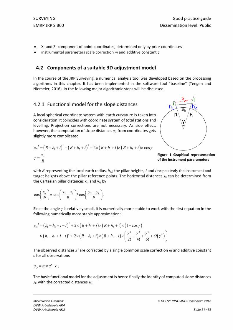
4.2.1 Functional model for the slope distances
A local spherical coordinate system with earth curvature is taken into consideration. It coincides with coordinate system of total stations and levelling. Projection corrections are not necessary. As side effect, however, the computation of slope distances sC from coordinates gets slightly more complicated
( ) ( ) ( ) ( )2 22
C 1 2 1 2
h
2 coss R h i R h t R h i R h t
s
R
γ
γ
= + + + + + − × + + × + + ×
=
with R representing the local earth radius, h1,2 the pillar heights, i and t respectively the instrument and target heights above the pillar reference points. The horizontal distances sh can be determined from the Cartesian pillar distances xi,j and yi,j by
2 1 2 1hcos cos *cosx x y y
R
s
RR
− − =
.
Since the angle γ is relatively small, it is numerically more stable to work with the first equation in the following numerically more stable approximation:
( ) ( ) ( ) ( )
( ) ( ) ( ) ( )
22
C 1 2 1 2
2 4 62 8
1 2 1 2
2 1 cos
22! 4! 6!
s h h i t R h i R h i
h h i t R h i R h i O
γ
γ γ γγ
= − + − + × + + × + + × −
≈ − + − + × + + × + + × − + +
The observed distances s’ are corrected by a single common scale correction m and additive constant c for all observations
O 's m s c= × + .
The basic functional model for the adjustment is hence finally the identity of computed slope distances sC with the corrected distances sO:
Figure 1 Graphical representation
of the instrument pararameters
c

SURVEYING Good practice guide
EMRP JRP SIB60 Dissemination level: Public
Mitwirkende Gremien: © SURVEYING JRP-Consortium 2016
DVW Arbeitskreis AK4
DVW Arbeitskreis AK3 Seite 32 / 53
!
O Cs s= .
4.2.2 Stochastic model for the observations
The 3D adjustment treats both the coordinate pillars and the observed distances as variables. The weighting between these observations must reflect the different uncertainties of this entrance data. The corrections deduced in the adjustment should be in the order of the assumed uncertainties. Larger deviations are an indication that the assumptions on the accuracy of the prior information should be reconsidered.
For the observed distances, prior accuracy information can be introduced either from previous calibrations or from specifications.
In case of the coordinates of the pillars, a covariance matrix Qxx,j for each pillar j should be introduced as derived from adjustment resp. determination of reference baseline coordinates /lengths.
���,� = ���� �� ��� ���
During the adjustment, the introduction of individual observation accuracies is a possible way to reweight blunders during the processing chain.
4.2.3 Correction of distances
It is mandatory to have corrections applied to the raw observations:
Atmospheric corrections:
• First velocity correction: determine the refractive index from temperature, air pressure, and relative humidity and the approximation formula (Ciddor/Bönsch).
• Beam curvature correction. Laser beam does not follow the chord between instrument and reflector, but follows a gentle arc with a radius 8 times larger than the earth radius (Rüeger, 1996)
• Second speed correction. Local scale refractive index depends on altitude. Following the gentle arc, the laser beam passes closer to earth surface in its midpath.
Geometrical corrections:
• If instrument and prism heights are different, parallax has to be considered.

SURVEYING Good practice guide
EMRP JRP SIB60 Dissemination level: Public
Mitwirkende Gremien: © SURVEYING JRP-Consortium 2016
DVW Arbeitskreis AK4
DVW Arbeitskreis AK3 Seite 33 / 53
4.2.4 Adjustment Model
A Gauss-Markov Model (Niemeier (2008)) can be used to determine the instrument parameter. The algorithms behind this analysis are sketched in the following:
Functional model:
�̂ = ����� This equation is relating the adjusted observations �̂ explicitly to the estimated parameters ��. The measured observations � have to be corrected by a residual �:
� + � = ����� The functional model is linearized explicitly by approximation to a first-order Taylor series expansion:
� + � = ����� = ����� + ��
where �� are a priori values of the parameters and �� are the estimated parameter corrections to the
a priori values: �� = �� + ��. The design matrix � = �������� ! contains the first derivative of function ���� with respect to parameters �.
� = ��� − �� − �����)
The linearized model with # = �� − �����) then reads
� = ��� − #
Stochastic model:
1
llP Q−=
The matrix �$$contains the covariance of the observations and the inverse matrix % is called the weight matrix.
Least square minimization:
�&%� = ���� − #�&%���� − #� → min
Leading to
0Tv Pv
x
∂=
∂
Solution:

SURVEYING Good practice guide
EMRP JRP SIB60 Dissemination level: Public
Mitwirkende Gremien: © SURVEYING JRP-Consortium 2016
DVW Arbeitskreis AK4
DVW Arbeitskreis AK3 Seite 34 / 53
( ) 1
ˆ T Tx A PA A Pl−
=
����� = ��&%��+, The matrix ����� contains the covariance of the adjusted parameters.

SURVEYING Good practice guide
EMRP JRP SIB60 Dissemination level: Public
Mitwirkende Gremien: © SURVEYING JRP-Consortium 2016
DVW Arbeitskreis AK4
DVW Arbeitskreis AK3 Seite 35 / 53
5 Measurement uncertainty
5.1 Survey on contributions
The calibration of offset and scale of an EDM is influenced by multiple uncertainty contributions. A survey is given in the Ishikawa diagram depicted in figure 2. According to GUM, all these contributions need to be quantified and their contribution to the calibration values determined by uncertainty propagation through the analysis. In this chapter, uncertainty magnitudes and a Monte Carlo based method for the determination of the expanded measurement uncertainty will be discussed.
Figure 2 Ishikawa diagram summarizing uncertainty contributions to the calibration process.
5.2 Influence of the refractive index
The uncertainty of the expressions by Ciddor or Bönsch and Potulski for the refractive index of air is at the level of a few parts in 10-8, but this requires temperature to be known within 10 mK, pressure within 4 Pa, relative humidity within 1 % and CO2 contents within 70 ppm. The uncertainty of the calibration of respective sensors is typically well below these. However, the uncertainty of the effective refractive index along the whole beam path is dominated by the challenge to sample the spatial and temporal gradients of these quantities directly.
SURVEYING Good practice guide
EMRP JRP SIB60 Dissemination level: Public
Mitwirkende Gremien: © SURVEYING JRP-Consortium 2016
DVW Arbeitskreis AK4
DVW Arbeitskreis AK3 Seite 36 / 53
For long distance surveying under rapidly changing conditions, a near continuous array of accurate and fast sensors would be needed exactly along the path of the EDM beam. The requirements for temperature and humidity are especially demanding. While substantial progress has been made in lessening the demands on temperature data by measuring at multiple wavelengths (Meiners-Hagen et al., 2016) and in realizing a spatially continuous measurement of temperature (Hieta et al., 2011) and humidity (Pollinger et al., 2012b) along the EDM path spectroscopically, these methods are not widely available yet. When the air parameters can only be measured at one or a few points around the EDM beam, knowledge of the size of gradients, especially for temperature, becomes very important for determining the measurement uncertainty.
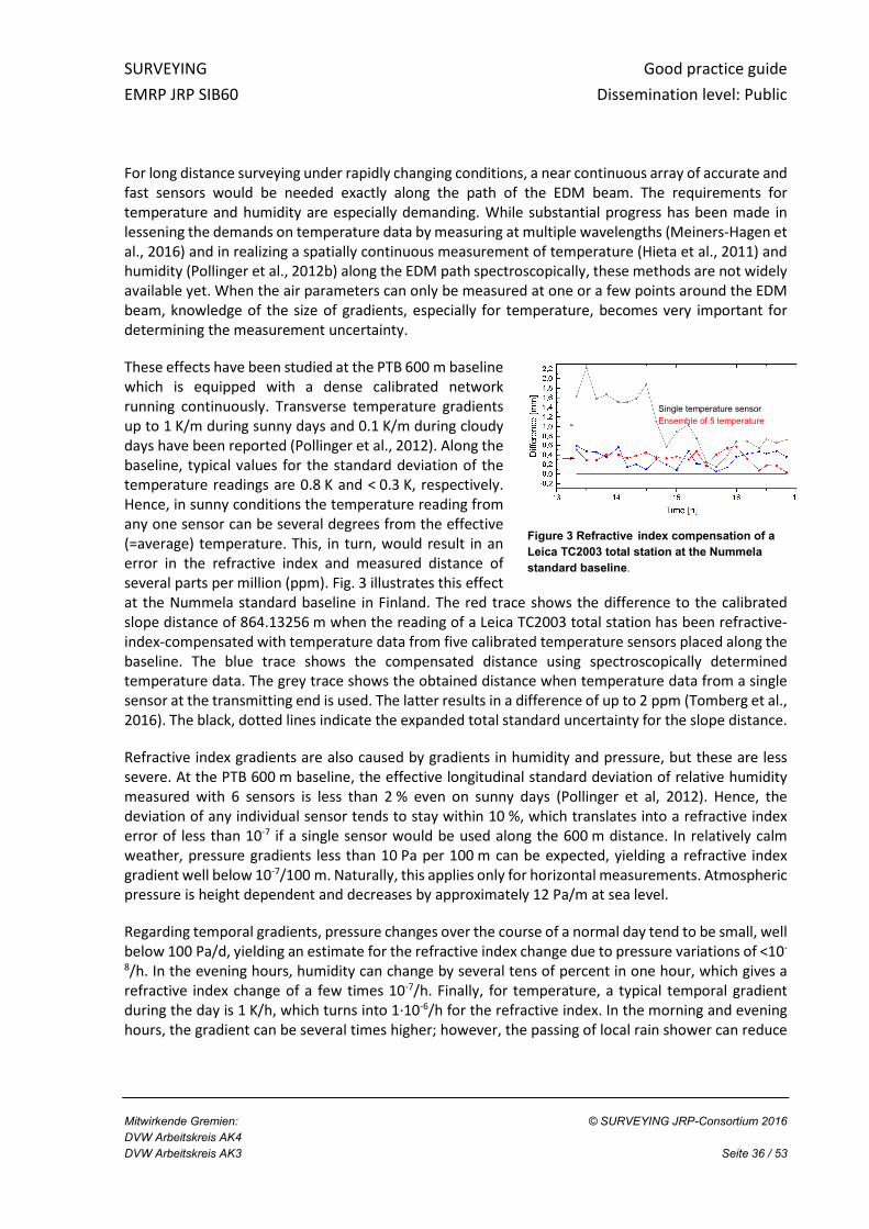
These effects have been studied at the PTB 600 m baseline which is equipped with a dense calibrated network running continuously. Transverse temperature gradients up to 1 K/m during sunny days and 0.1 K/m during cloudy days have been reported (Pollinger et al., 2012). Along the baseline, typical values for the standard deviation of the temperature readings are 0.8 K and < 0.3 K, respectively. Hence, in sunny conditions the temperature reading from any one sensor can be several degrees from the effective (=average) temperature. This, in turn, would result in an error in the refractive index and measured distance of several parts per million (ppm). Fig. 3 illustrates this effect at the Nummela standard baseline in Finland. The red trace shows the difference to the calibrated slope distance of 864.13256 m when the reading of a Leica TC2003 total station has been refractive-index-compensated with temperature data from five calibrated temperature sensors placed along the baseline. The blue trace shows the compensated distance using spectroscopically determined temperature data. The grey trace shows the obtained distance when temperature data from a single sensor at the transmitting end is used. The latter results in a difference of up to 2 ppm (Tomberg et al., 2016). The black, dotted lines indicate the expanded total standard uncertainty for the slope distance.
Refractive index gradients are also caused by gradients in humidity and pressure, but these are less severe. At the PTB 600 m baseline, the effective longitudinal standard deviation of relative humidity measured with 6 sensors is less than 2 % even on sunny days (Pollinger et al, 2012). Hence, the deviation of any individual sensor tends to stay within 10 %, which translates into a refractive index error of less than 10-7 if a single sensor would be used along the 600 m distance. In relatively calm weather, pressure gradients less than 10 Pa per 100 m can be expected, yielding a refractive index gradient well below 10-7/100 m. Naturally, this applies only for horizontal measurements. Atmospheric pressure is height dependent and decreases by approximately 12 Pa/m at sea level.
Regarding temporal gradients, pressure changes over the course of a normal day tend to be small, well below 100 Pa/d, yielding an estimate for the refractive index change due to pressure variations of <10-
8/h. In the evening hours, humidity can change by several tens of percent in one hour, which gives a refractive index change of a few times 10-7/h. Finally, for temperature, a typical temporal gradient during the day is 1 K/h, which turns into 1∙10-6/h for the refractive index. In the morning and evening hours, the gradient can be several times higher; however, the passing of local rain shower can reduce
Figure 3 Refractive index compensation of a
Leica TC2003 total station at the Nummela
standard baseline.
Single temperature sensor
Ensemble of 5 temperature
sensors
SURVEYING Good practice guide
EMRP JRP SIB60 Dissemination level: Public
Mitwirkende Gremien: © SURVEYING JRP-Consortium 2016
DVW Arbeitskreis AK4
DVW Arbeitskreis AK3 Seite 37 / 53
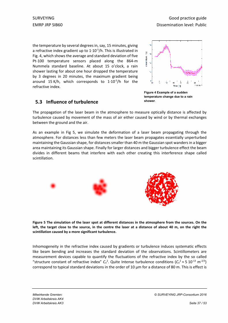
the temperature by several degrees in, say, 15 minutes, giving a refractive index gradient up to 1∙10-5/h. This is illustrated in Fig. 4, which shows the average and standard deviation of five Pt-100 temperature sensors placed along the 864-m Nummela standard baseline. At about 15 o’clock, a rain shower lasting for about one hour dropped the temperature by 3 degrees in 20 minutes, the maximum gradient being around 15 K/h, which corresponds to 1∙10-5/h for the refractive index.
5.3 Influence of turbulence
The propagation of the laser beam in the atmosphere to measure optically distance is affected by turbulence caused by movement of the mass of air either caused by wind or by thermal exchanges between the ground and the air.
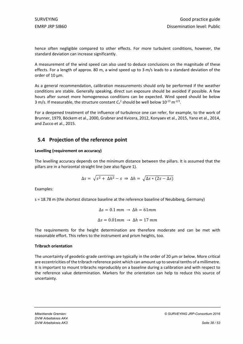
As an example in Fig 5, we simulate the deformation of a laser beam propagating through the atmosphere. For distances less than few meters the laser beam propagates essentially unperturbed maintaining the Gaussian shape, for distances smaller than 40 m the Gaussian spot wanders in a bigger area maintaining its Gaussian shape. Finally for larger distances and bigger turbulence effect the beam divides in different beams that interfere with each other creating this interference shape called scintillation.
Figure 5 The simulation of the laser spot at different distances in the atmosphere from the sources. On the
left, the target close to the source, in the centre the laser at a distance of about 40 m, on the right the
scintillation caused by a more significant turbulence.
Inhomogeneity in the refractive index caused by gradients or turbulence induces systematic effects like beam bending and increases the standard deviation of the observations. Scintillometers are measurement devices capable to quantify the fluctuations of the refractive index by the so called “structure constant of refractive index” Cn
2. Quite Intense turbulence conditions (Cn2 ≈ 5 10-13 m-2/3)
correspond to typical standard deviations in the order of 10 µm for a distance of 80 m. This is effect is
Figure 4 Example of a sudden
temperature change due to a rain
shower.
SURVEYING Good practice guide
EMRP JRP SIB60 Dissemination level: Public
Mitwirkende Gremien: © SURVEYING JRP-Consortium 2016
DVW Arbeitskreis AK4
DVW Arbeitskreis AK3 Seite 38 / 53
hence often negligible compared to other effects. For more turbulent conditions, however, the standard deviation can increase significantly.
A measurement of the wind speed can also used to deduce conclusions on the magnitude of these effects. For a length of approx. 80 m, a wind speed up to 3 m/s leads to a standard deviation of the order of 10 µm.
As a general recommendation, calibration measurements should only be performed if the weather conditions are stable. Generally speaking, direct sun exposure should be avoided if possible. A few hours after sunset more homogeneous conditions can be expected. Wind speed should be below 3 m/s. If measurable, the structure constant Cn
2 should be well below 10-13 m-2/3.
For a deepened treatment of the influence of turbulence one can refer, for example, to the work of Brunner, 1979, Böckem et al., 2000, Grabner and Kvicera, 2012, Konyaev et al., 2015, Yano et al., 2014, and Zucco et al., 2015.
5.4 Projection of the reference point
Levelling (requirement on accuracy)
The levelling accuracy depends on the minimum distance between the pillars. It is assumed that the pillars are in a horizontal straight line (see also figure 1).
∆� = .�/ + ∆ℎ/ − � ⇒ ∆ℎ = .∆� ∗ �2� − ∆��
Examples:
s = 18.78 m (the shortest distance baseline at the reference baseline of Neubiberg, Germany)
∆� = 0.1 77 → ∆ℎ = 6177
∆� = 0.0177 → ∆ℎ = 17 77
The requirements for the height determination are therefore moderate and can be met with reasonable effort. This refers to the instrument and prism heights, too.
Tribrach orientation
The uncertainty of geodetic-grade centrings are typically in the order of 20 µm or below. More critical are eccentricities of the tribrach reference point which can amount up to several tenths of a millimetre. It is important to mount tribrachs reproducibly on a baseline during a calibration and with respect to the reference value determination. Markers for the orientation can help to reduce this source of uncertainty.

SURVEYING Good practice guide
EMRP JRP SIB60 Dissemination level: Public
Mitwirkende Gremien: © SURVEYING JRP-Consortium 2016
DVW Arbeitskreis AK4
DVW Arbeitskreis AK3 Seite 39 / 53
Levelling the individual tribrachs should be performed with high quality geodetic laser plummets with two perpendicular tubular levels. For typical uncertainties in the order of 30 arcseconds, length deviations due to tilted EDMs and reflectors can be reduced to the order of 40 µm.
5.5 Uncertainty estimate of the calibration parameters
Uncertainty propagation for a 3D adjustment as discussed in chapter 4.2 is not straightforward. Monte Carlo methods which numerically repeat the analysis with randomly varying starting conditions are a suitable and well-established tool to propagate the contributing uncertainties.
Nowadays with efficient computers and good random number generators large samples are possible. Input variability is computed by deterministic, pseudorandom sequences, making it easy to test and re-run simulations.
One algorithm for the implementation of such an uncertainty propagation could be:
• Define the functional relation between input data and quantity of interest (see chapter 4.2).
• Use the uncertainty assessment of the various contributing quantities to define a domain of
possible input data.
• Generate input data randomly from a probability distribution over the domain.
• Perform a deterministic computation on the inputs and get the quantities of interest.
• Aggregate and analyze the computed quantities of interest.
To demonstrate achievable measurement uncertainties for a calibration measurement, this procedure was performed for measurements at the baseline of PTB Braunschweig in the following discussion.
Each simulation consists of 1000 runs of the adjustment. Each time a new set of points and observations is generated. A forced centring is assumed so the coordinates may differ in each simulation according to the pillar centring variations. As a result the scale and the additional constant are determined in each run.
Steps per run:
• Adopt centring variations to pillar coordinates
• Consider instrument and target height
• Calculate observations from coordinates
o Uncertainties of calibration data for EDM
o Uncertainties of atmospheric data for EDM
o Instrument accuracy
• Adjust the observations
• Store the results of the adjustment
The data of each run are collected. The results are stored in a vector, sorted by value and the following values are determined:
SURVEYING Good practice guide
EMRP JRP SIB60 Dissemination level: Public
Mitwirkende Gremien: © SURVEYING JRP-Consortium 2016
DVW Arbeitskreis AK4
DVW Arbeitskreis AK3 Seite 40 / 53
• 2,5 % lower limit 95 % significance level
• 16 % lower limit 68 % significance level, one standard deviation
• 50 % Median
• 84 % upper limit 68 % significance level, one standard deviation
• 97,5 % upper limit 95 % significance level
It should be noted that the quantiles can be interpreted independent from the distribution.
Based on the considerations before, the following entrance parameters were chosen for the uncertainty propagation:
Type A: based on statistical analysis of real observations during the measurement
In a real calibration measurement, the following quantities are acquired by multiple measurements. The derived mean value and standard deviation enter into the adjustment. For the simulations, also these “observations” were simulated based on the following assumptions for the uncertainties:
- Observed distances: Every EDM under test is imperfect, e.g. due to electronic noise or mechanical design stability. The quality of the observation data limits of course also the uncertainty of the achievable correction parameters. To account for this effect, a selection of devices of typical different accuracy grades has been used for the simulations (c is the additional constant and m the scale factor):
Instrument Standard deviation of c [mm]
Standard deviation of m [ppm]
Ideal 0.0 0.0
ME 5000 0.2 0.2
EDM A 0.6 1.0
EDM B 1.0 2.0
EDM C 2.0 2.0
- Atmospheric Parameters: The atmospheric parameters are observed by a temperature network. For the simulations, the following uncertainties and distributions are assumed reflecting the difficulty in sampling them with sufficient accuracy: Temperature: uniform distribution, σ = 0.8 K; 1 K ≈ 1 ppm
Pressure: uniform distribution, σ = 0.5 mbar; 1 mbar ≈ 0.3 ppm
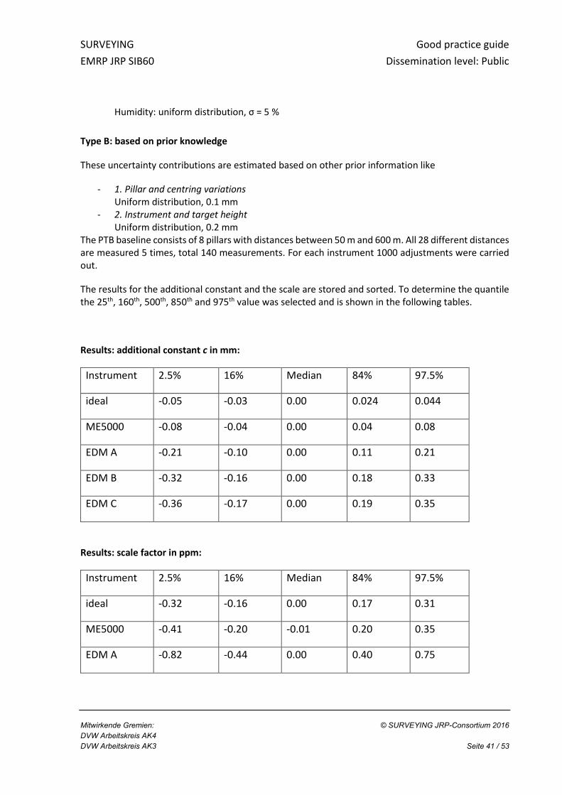
SURVEYING Good practice guide
EMRP JRP SIB60 Dissemination level: Public
Mitwirkende Gremien: © SURVEYING JRP-Consortium 2016
DVW Arbeitskreis AK4
DVW Arbeitskreis AK3 Seite 41 / 53
Humidity: uniform distribution, σ = 5 %
Type B: based on prior knowledge
These uncertainty contributions are estimated based on other prior information like
- 1. Pillar and centring variations
Uniform distribution, 0.1 mm - 2. Instrument and target height
Uniform distribution, 0.2 mm The PTB baseline consists of 8 pillars with distances between 50 m and 600 m. All 28 different distances are measured 5 times, total 140 measurements. For each instrument 1000 adjustments were carried out.
The results for the additional constant and the scale are stored and sorted. To determine the quantile the 25th, 160th, 500th, 850th and 975th value was selected and is shown in the following tables.
Results: additional constant c in mm:
Instrument 2.5% 16% Median 84% 97.5%
ideal -0.05 -0.03 0.00 0.024 0.044
ME5000 -0.08 -0.04 0.00 0.04 0.08
EDM A -0.21 -0.10 0.00 0.11 0.21
EDM B -0.32 -0.16 0.00 0.18 0.33
EDM C -0.36 -0.17 0.00 0.19 0.35
Results: scale factor in ppm:
Instrument 2.5% 16% Median 84% 97.5%
ideal -0.32 -0.16 0.00 0.17 0.31
ME5000 -0.41 -0.20 -0.01 0.20 0.35
EDM A -0.82 -0.44 0.00 0.40 0.75

SURVEYING Good practice guide
EMRP JRP SIB60 Dissemination level: Public
Mitwirkende Gremien: © SURVEYING JRP-Consortium 2016
DVW Arbeitskreis AK4
DVW Arbeitskreis AK3 Seite 42 / 53
EDM B -1.02 -0.64 -0.01 0.56 1.12
EDM C -1.39 -0.74 -0.02 0.68 1.29
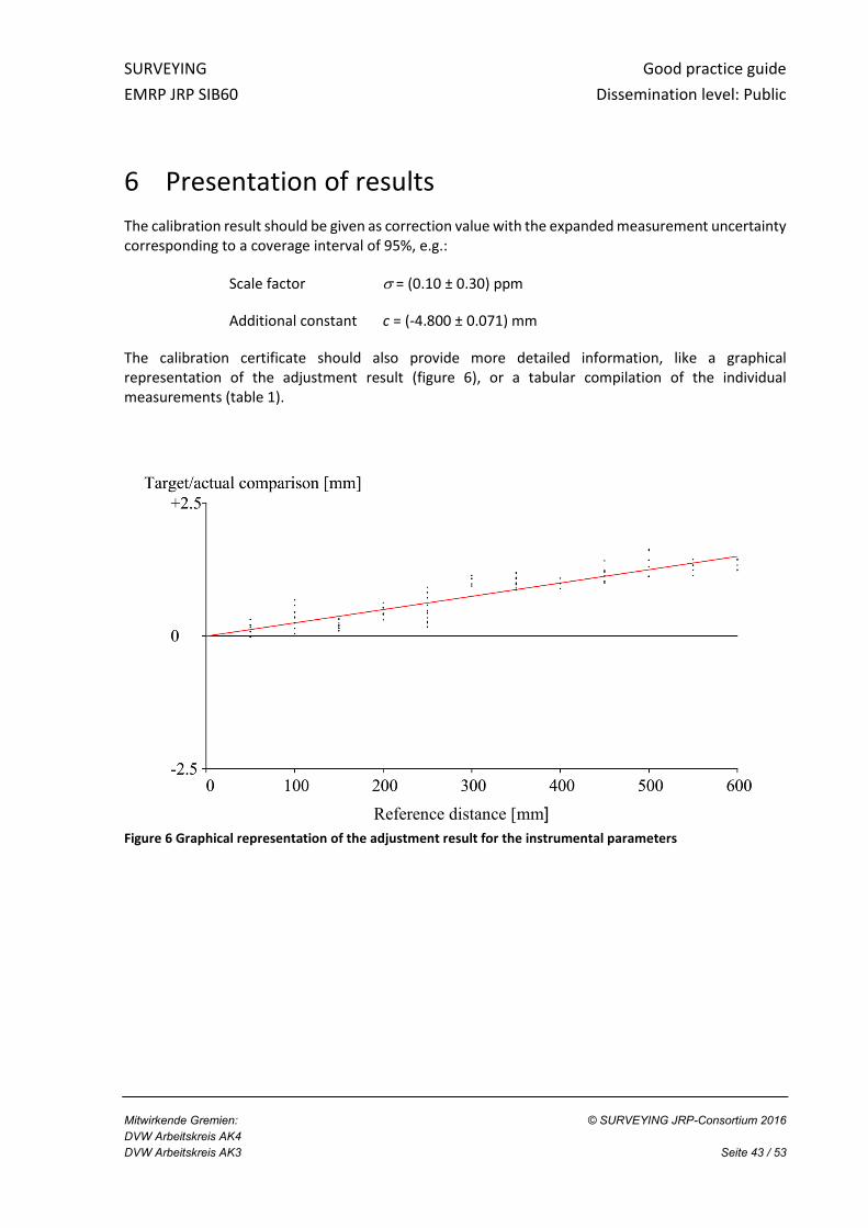
SURVEYING Good practice guide
EMRP JRP SIB60 Dissemination level: Public
Mitwirkende Gremien: © SURVEYING JRP-Consortium 2016
DVW Arbeitskreis AK4
DVW Arbeitskreis AK3 Seite 43 / 53
6 Presentation of results
The calibration result should be given as correction value with the expanded measurement uncertainty corresponding to a coverage interval of 95%, e.g.:
Scale factor σ = (0.10 ± 0.30) ppm
Additional constant c = (-4.800 ± 0.071) mm
The calibration certificate should also provide more detailed information, like a graphical representation of the adjustment result (figure 6), or a tabular compilation of the individual measurements (table 1).
Figure 6 Graphical representation of the adjustment result for the instrumental parameters
Reference distance [mm]
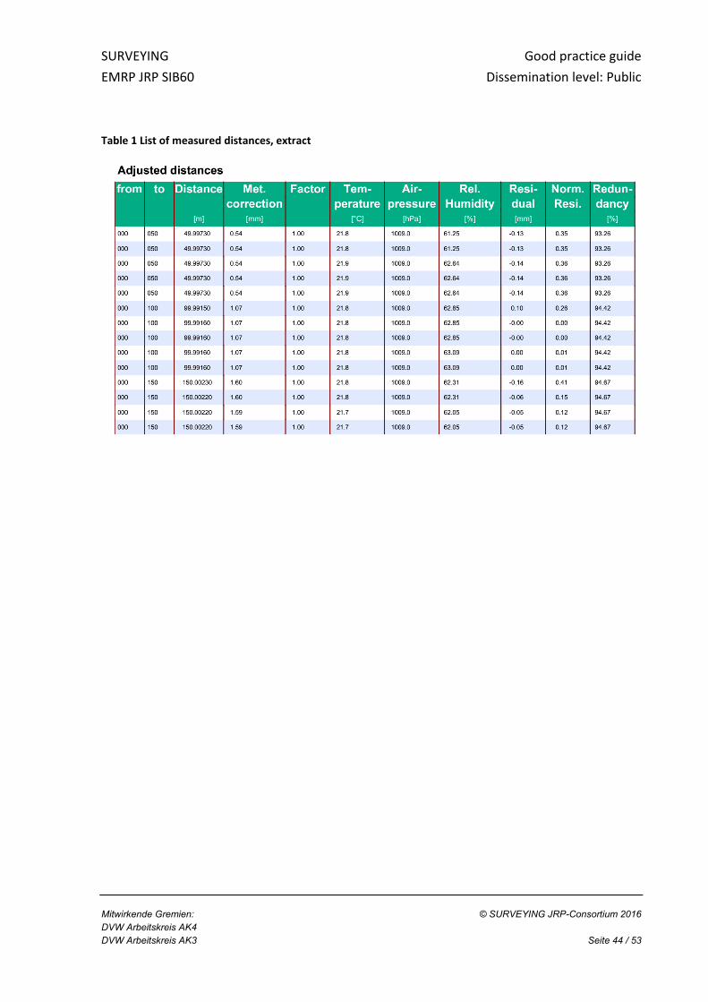
SURVEYING Good practice guide
EMRP JRP SIB60 Dissemination level: Public
Mitwirkende Gremien: © SURVEYING JRP-Consortium 2016
DVW Arbeitskreis AK4
DVW Arbeitskreis AK3 Seite 44 / 53
Table 1 List of measured distances, extract

SURVEYING Good practice guide
EMRP JRP SIB60 Dissemination level: Public
Mitwirkende Gremien: © SURVEYING JRP-Consortium 2016
DVW Arbeitskreis AK4
DVW Arbeitskreis AK3 Seite 45 / 53
7 Appendix
7.1 Field book
The following field book realized in a spreadsheet program collects all information required for the analysis of the calibration measurement.
Figure 7 General data
observers:
home institutes:
all clocks synchronised: yes
EDM:
automated data aquisition: no
reflector:
targeting method: manual
calibrated device: yes
calibration date:
calibration factors: offset / m: scale factor: further:
standard pressure / hPa:
standard temperature / °C:
standard humidity / %rf:
baseline:
baseline orientation with
respect to the starting point:
nominal pillar positions / m 0 50 100 150 250 350 500 600
centring method:
centring uncertainty (k=1):
level for alignment: type:
device height over reference
point / m
reflector height over reference
point / m
measurement date
Dates and operators
operators
uncertainty / m (k=1):
uncertainty / m (k=1):
uncertainty / deg (k=1):
Baseline data
Mounting and Alignment
Measurement method
Measurement method
Environmental correction - please use standard atmosphere!
calibration laboratory:
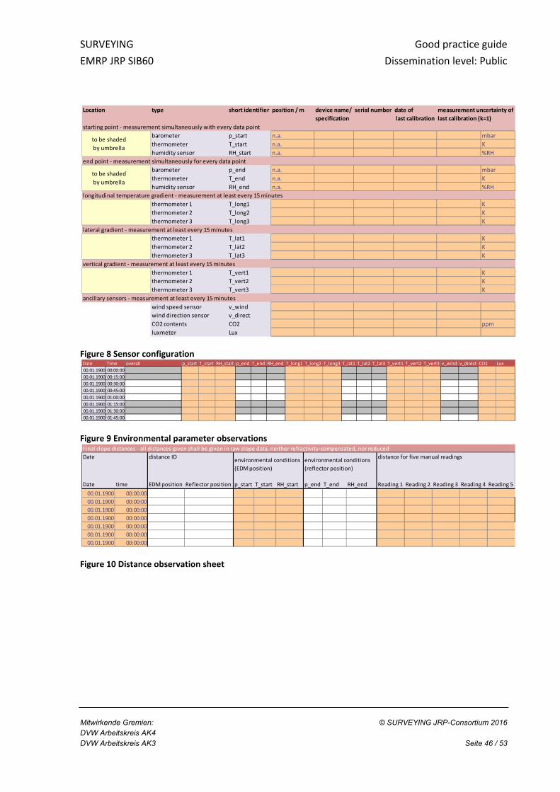
SURVEYING Good practice guide
EMRP JRP SIB60 Dissemination level: Public
Mitwirkende Gremien: © SURVEYING JRP-Consortium 2016
DVW Arbeitskreis AK4
DVW Arbeitskreis AK3 Seite 46 / 53
Figure 8 Sensor configuration
Figure 9 Environmental parameter observations
Figure 10 Distance observation sheet
Location type short identifier position / m device name/
specification
serial number date of
last calibration
starting point - measurement simultaneously with every data point
barometer p_start n.a. mbar
thermometer T_start n.a. K
humidity sensor RH_start n.a. %RH
barometer p_end n.a. mbar
thermometer T_end n.a. K
humidity sensor RH_end n.a. %RH
thermometer 1 T_long1 K
thermometer 2 T_long2 K
thermometer 3 T_long3 K
thermometer 1 T_lat1 K
thermometer 2 T_lat2 K
thermometer 3 T_lat3 K
thermometer 1 T_vert1 K
thermometer 2 T_vert2 K
thermometer 3 T_vert3 K
wind speed sensor v_wind
wind direction sensor v_direct
CO2 contents CO2 ppm
luxmeter Lux
measurement uncertainty of
last calibration (k=1)
end point - measurement simultaneously for every data point
longitudinal temperature gradient - measurement at least every 15 minutes
lateral gradient - measurement at least every 15 minutes
ancillary sensors - measurement at least every 15 minutes
to be shaded
by umbrella
to be shaded
by umbrella
vertical gradient - measurement at least every 15 minutes
Date Time overall p_start T_start RH_start p_end T_end RH_end T_long1 T_long2 T_long3 T_lat1 T_lat2 T_lat3 T_vert1 T_vert2 T_vert3 v_wind v_direct CO2 Lux
00.01.1900 00:00:00
00.01.1900 00:15:00
00.01.1900 00:30:00
00.01.1900 00:45:00
00.01.1900 01:00:00
00.01.1900 01:15:00
00.01.1900 01:30:00
00.01.1900 01:45:00
Final slope distances - all distances given shall be given in raw slope data, neither refractivity-compensated, nor reduced
Date time EDM position Reflector position p_start T_start RH_start p_end T_end RH_end Reading 1 Reading 2 Reading 3 Reading 4 Reading 5
00.01.1900 00:00:00
00.01.1900 00:00:00
00.01.1900 00:00:00
00.01.1900 00:00:00
00.01.1900 00:00:00
00.01.1900 00:00:00
00.01.1900 00:00:00
distance IDenvironmental conditions
(EDM position)
Dateenvironmental conditions
(reflector position)
distance for five manual readings
SURVEYING Good practice guide
EMRP JRP SIB60 Dissemination level: Public
Mitwirkende Gremien: © SURVEYING JRP-Consortium 2016
DVW Arbeitskreis AK4
DVW Arbeitskreis AK3 Seite 47 / 53
7.2 On traceability
7.2.1 Traceability chain: the example of the Nummela scale transfer
The establishment of traceability to the SI definition of the metre for reference lengths of baselines with low uncertainty is non-trivial. In this section, the approach of the Finnish Geospatial Research Institute (FGI) is introduced. The so-called Nummela scale transfer is an internationally acknowledged calibration service for geodetic baselines. It also demonstrates the increase of uncertainties in the different steps of the traceability chain.
The national metrology institute of Finland, VTT MIKES Metrology, performs the high-level realization of the definition of the metre using internationally recommended methods. VTT also calibrates FGI’s 1-metre-long quartz gauges, which transfer the traceable scale to FGI’s Väisälä interference comparator. A measurement setup and procedure combining white light and laser light in an interferometer for long gauge blocks is used (Lassila et al. 2003).
The length of a quartz gauge, known with 35 nm standard uncertainty, is multiplied in the (white-light) Väisälä interference comparator to realise longer distances. The design of FGI’s Nummela Standard Baseline allows a multiplication of 2 x 2 x 3 x 3 x 4 x 6 x 1 m = 864 m. Typical standard uncertainties are from 0.03 mm to 0.08 mm for the baseline lengths from 24 m to 864 m (Jokela 2014).
Projection measurements transfer the lengths between underground baseline benchmarks to lengths between centring equipment on above ground observation pillars, which are used in EDM calibrations. Owing to the optimal measurement geometry and best available measurement instruments the standard uncertainties after the projections remain smaller than 0.2 mm.
The FGI mostly uses a Kern ME5000 high-precision EDM equipment as a transfer standard for traceable scale transfer from Nummela to other geodetic baselines. The transfer standard is calibrated a few times at Nummela before and after the measurement at the scale transfer site, accompanied by before and after projections at Nummela. Figure 11 shows the procedure in more detail.
In processing meteorological data for EDM the FGI uses a computation method first proposed by Ciddor (1996), as recommended by the International Association of Geodesy (IAG, 2000). If using some of the formulas presented in the Kern ME5000 manual (Owens, Edlen, Barrel & Sears) instead, differences of up to 0.1 mm may occur in corrections.

SURVEYING Good practice guide
EMRP JRP SIB60 Dissemination level: Public
Mitwirkende Gremien: © SURVEYING JRP-Consortium 2016
DVW Arbeitskreis AK4
DVW Arbeitskreis AK3 Seite 48 / 53
Figure 11 Overview of calibration of transfer standard for scale transfer (Jokela 2014)
7.2.2 Alternative optical standards for the primary realisation of the SI unit metre in surveying
As mentioned in 1.1, even if an optical instrument is capable of measuring somehow the time of flight of a light beam between two points with an accuracy as high as possible, the estimation of the distance between these points will be degraded by the way of estimating the speed of light between these points. The classical way is based on local sensors that are expected to give estimation as close as possible of the effective atmospheric parameters all along the light beam. But even with a large effort in the sensor network, the uncertainty of such a sensor-based approximation of the effective environmental parameters remains limited (see chapter 5.1). Spectroscopic sampling of the effective environmental parameters can reduce the uncertainty significantly (Hieta, 2011).
Another alternative is to use the dispersion of air index (known thanks to air index formulas) between two separate wavelengths. By measuring the same distance simultaneously at two different wavelengths, the “true” i.e. geometric distance can be deduced without measuring neither the air
temperature nor the air pressure. If L1 is the distance measured at wavelength λ1 (taking the air index
equal to unity), L2 the distance measured at wavelength λ2 (taking the air index equal to unity), the true distance L can be written as follow (with minor simplification):
L=L1+A(λ1 , λ2 )x(L2-L1)
The A factor is a quantity deduced from air index formulas and that depends only on the value of the
two wavelengths chosen for the measurement (for λ1=1064 nm and λ2=532 nm A is equal to 21). This
Weather variations along
the path of measurement ?
Stability of the baseline ?
National standard baseline
section lengths (between
underground markers)
Projection measurements
for calibrations
National standard
baseline section lengths
(aboveground, between
observation pillars)
EDM instrument observations
for calibration (including
centring, levelling, targetting etc.)
Weather observations
(t, p, rh%, CO2)
Instrument corrections
for weather observations
Height differences
for geometrical corrections
Observed and corrected
baseline section lengths
Comparison,
weighted
least-squares
adjustment
EDM
instrument corrections
for the transfer standard
• scale correction,
• additive constant,
• possible other;
• stability of results
(calibrations before/after)?
Computation formulas
for corrections for distances
Similar measurements
and computations using the
calibrated transfer standard
at the transfer site
Calibration programme
Calibration history
(time series)
SURVEYING Good practice guide
EMRP JRP SIB60 Dissemination level: Public
Mitwirkende Gremien: © SURVEYING JRP-Consortium 2016
DVW Arbeitskreis AK4
DVW Arbeitskreis AK3 Seite 49 / 53
A factor acts also as an amplification factor of the dispersion of the distance measurement: the dispersion on (L2-L1) measurement is amplified by this factor A. This is the price to pay for air index compensation: the uncertainty on L2-L1 should be A times better than the global uncertainty reached for the true distance. In the past, several units of such a device, known as Terrameter (Hugget, 1981) were realized and used for some critical applications. The principle of operation with millimetre level accuracy was demonstrated but no such instrument is in operation today.
Within the frame of the JRP Surveying this approach was revived using modern optical and recent advances in laser technology. The “TeleYAG” system (Meiners-Hagen et al., 2015) is a primary standard for baseline calibrations with measurement uncertainties on sub-millimetre level. It is now used in the German national metrology institute for the calibration of their baseline. A stronger focus on transportability and user-friendliness was put on the parallel not yet completed development of the TeleDiode system based on optoelectronic fibre technology (Guillory et al., 2016). The developers see the potential of the design to make an operational transportable instrument available to a broader application group in a near future.
SURVEYING Good practice guide
EMRP JRP SIB60 Dissemination level: Public
Mitwirkende Gremien: © SURVEYING JRP-Consortium 2016
DVW Arbeitskreis AK4
DVW Arbeitskreis AK3 Seite 50 / 53
8 Literature
Bönsch, G.; Potulski, E (1998). Measurement of the refractive index of air and comparison with modified Edlén's formulae. Metrologia 35, 133-139
Böckem, B.; Flach, P.; Weiss, A.; Hennes, M. (2000). Refraction influence analysis and investigations on automated elimination of refraction effects on geodetic measurements. Proc. of XVI IMEKO World Congress 2000
Brunner F.K. (1979). Vertical refraction angle derived from the variance of the angle-of-arrival fluctuations. Refractional Influences in Astrometry and Geodesy, pp. 227-238
Ciddor, P. E.; Hill, R. J. (1999): Refractive index of air: 2. Group index. Applied Optics, 38(1999)9, 1663-1667.
Ciddor, P. E. (2002): Refractive index of air: 3. The roles of CO2, H2O, and refractivity virials. Applied Optics, Vol. 41, No. 12, 2292-2298, 2002
Ciddor, P. E. (1996). Refractive index of air: New equations for the visible and near infrared, Appl. Opt. 35:9, 1566–1573.
DVW-Merkblatt 8 (2014). Vermessungspfeiler. Available online under http://www.dvw.de/dvw-iso/17515/vermessungspfeiler
Eschelbach, C. (2009). Refraktionskorrekturbestimmung durch Modellierung des Impuls und Wärmeflusses in der Rauhigkeitsschicht, Dissertation, Schriftenreihe des Studiengangs Geodäsie und Geoinformatik, Universität Karlsruhe (TH), Heft-Nr. 2009/1. 2009.
Grabner, M.; Kvicera V. (2012). Measurement of the Structure Constant of Refractivity at Optical Wavelengths Using a Scintillometer. Radioengineering 21, pp. 455-458
Guillory, J.; Šmid, R.; Garcia-Marquez, J.; Truong, D.; Alexandre, C.; Wallerand, J.-P. (2016). High resolution kilometric range optical telemetry in air by radio frequency phase measurement Review of Scientific Instruments 87, 075105
Heister, H. (2012): Die neuen Kalibrierbasis der UniBW München. AVN, 10/2012, p 336-343
Heunecke,O. (2015). Die neue Neubiberger Pfeilerstrecke, In: Zeitschrift für Geodäsie, Geoinformation und Landmanagement, ZFV, 2015, pp. 357-364.
Hieta, T.; Merimaa, M.; Vainio, M.; Seppä, J.; Lassila, A. (2011). High-precision diode-laser-based temperature measurement for air refractive index compensation Appl. Opt., , 50, pp. 5990-5998
Huggett, G (1981), Two-color terrameter, Tectonophysics 71, pp. 29 - 39
IAG (2000). IAG Resolution 3 adopted at the XXIIth General Assembly in Birmingham. J. Geodesy 74:1, 66–67.
ISO 17123-1:2010, Optics and optical instruments – Field procedures for testing geodetic and surveying instruments – Part 1: Theory (2010)
ISO 17123-4:2012, , Optics and optical instruments – Field procedures for testing geodetic and surveying instruments – Part 4: Electro-optical distance meters (EDM measurement to reflectors)

SURVEYING Good practice guide
EMRP JRP SIB60 Dissemination level: Public
Mitwirkende Gremien: © SURVEYING JRP-Consortium 2016
DVW Arbeitskreis AK4
DVW Arbeitskreis AK3 Seite 51 / 53
ISO/IEC Guide 98-3:2008, Uncertainty of measurement – Part 3: Guide to the expression of uncertainty in measurement (GUM:1995)
Jokela, J. (2014). Length in Geodesy – On Metrological Traceability of a Geospatial Measurand. Publ. Finn. Geod. Inst. 154. 240 p.
Konyaev, P. A.; Botygina N. N.; Antoshkin, L.V.; Emaleev, O.N.; Lukin, V. P. (2015). On Atmospheric Turbulence Structure Constant Measurements by a Passive Optical Method. Proc. SPIE Vol 9680, 968024
Lassila, A., Jokela, J., Poutanen, M., Xu, J. (2003). Absolute calibration of quartz bars of Väisälä interferometer by white light gauge block interferometer. Proc. XVII IMEKO World Congress, June 22–27, 2003, Dubrovnik, Croatia, p. 1886–1890.
Meiners-Hagen, K.; Bosnjakovic, A.; Köchert, P.; Pollinger, F. (2015). Air index compensated interferometer as a prospective novel primary standard for baseline calibrations. Measurement Science and Technology 26, 084002
Meiners-Hagen, K.; Meyer, T.; Mildner, J.; Pollinger, F. (2016). Traceable Realization of geodetic distances with low uncertainty. In preparation
Niemeier (2008): Ausgleichungsrechnung – Statistische Auswertemethoden. Lehrbuch, 2. Auflage, deGruyter Verlag, Berlin
Pollinger, F.; Meyer, T.; Beyer, J.; Doloca, N. R.; Schellin, W.; Niemeier, W.; Jokela, J.; Häkli, P.; Abou-Zeid, A.; Meiners-Hagen, K. (2012). The upgraded PTB 600 m baseline: A high-accuracy reference for the calibration and the development of lomg distance measurement devices, Measurement Science and Technology 23, 094018
Pollinger, F.; Hieta, T.; Vainio, M.; Doloca, N. R.; Abou-Zeid, A.; Meiners-Hagen, K.; Merimaa, M. (2012b). Effective humidity in length measurements: comparison of three approaches, Measurement Science and Technology 23, 02550
Rüeger, J.M. (1996). Electronic Distance Measurement, 4th edn, Berlin: Springer
Schwarz, W. (2012). Einflussgrößen bei elektrooptischen Distanzmessungen und ihre Erfassung. AVN, 10/2012, p 323-335
Tengen, D.; Niemeier W. (2016). Baseline. Software tool, Technical University of Braunschweig, Germany
Tomberg, T.; Fordell, T.; J. Jokela; Merimaa, M.; T. Hieta (2016). Spectroscopic thermometry for long distance surveying, In preparation
Yano, K.; Yoshihisa, T.; Gyoda, K. (2014). Measurements of the Refractive Index Structure Constant and Studies on Beam wander. Proc. International Conference on Space Optical Systems and Applications (ICSOS) 2014, P-15, Kobe, Japan, May 7-9 (2014)
Zucco, M.; Pisani, M.; Astrua, M. (2015). Characterization of the effects of the turbulence on the propagation of a laser beam in air. Proc. CIM 2015, 17th International Congress of Metrology Paris, (September 21, 2015). DOI: http://dx.doi.org/10.1051/metrology/20150013014

SURVEYING Good practice guide
EMRP JRP SIB60 Dissemination level: Public
Mitwirkende Gremien: © SURVEYING JRP-Consortium 2016
DVW Arbeitskreis AK4
DVW Arbeitskreis AK3 Seite 52 / 53
Acknowledgements
We gratefully acknowledge funding from the European Metrology Research Program (EMRP). The EMRP is jointly funded by the EMRP participating countries within EURAMET and the European Union.
DVW-Merkblatt 10-2017
Metrology for long distance surveying with GNSS and EDM
Metrologie für die Enternungsmessung mit GNSS und EDM
Mitwirkende Gremien: Ersteller:
DVW Arbeitskreis AK4
DVW Arbeitskreis AK3 Heiner Kuhlmann Seite 53 / 53
Impressum
Herausgeber
DVW - Gesellschaft für Geodäsie, Geoinformation und Landmanagement e.V.
Geschäftsstelle
D-79235 Vogtsburg
Telefon: +49 7662/949287
Fax: +49 7662 / 949288
E-Mail: [email protected]


![DIGITAL VIDEOCASSETTE RECORDER DVW-M2000 DVW … · 2010-12-24 · DIGITAL VIDEOCASSETTE RECORDER DVW-M2000 DVW-M2000P DVW-2000 DVW-2000P TM OPERATION MANUAL [English] 1st Edition](https://img.pdfslide.net/doc/110x75/5e74dd6a7d2e605dc1239f9d/digital-videocassette-recorder-dvw-m2000-dvw-2010-12-24-digital-videocassette.jpg)