1

MESH TYPE AND NUMBER FOR CFD SIMULATIONS OF AIR 1 DISTRIBUTION IN AN AIRCRAFT CABIN 2

Ran Duan1, Wei Liu1, Luyi Xu1, Yan Huang1, Xiong Shen1, Chao-Hsin Lin2, Junjie Liu1, 3 Qingyan Chen3,1 and Balasubramanyam Sasanapuri4 4

5 1Tianjin Key Laboratory of Indoor Air Environmental Quality Control, School of Environmental 6

Science and Engineering, Tianjin University, Tianjin 300072, China 7 2Environmental Control Systems, Boeing Commercial Airplanes, Everett, WA 98203, USA 8

3School of Mechanical Engineering, Purdue University, West Lafayette, IN 47907, USA 9 4ANSYS India Pvt Ltd, Pune, India 10

11 This investigation evaluated the impact of three mesh types (hexahedral, tetrahedral, and hybrid 12 cells) and five grid numbers (3, 6, 12, 24, and >38 million cells) on the accuracy and computing 13 costs of air distribution simulations in a first-class cabin. This study performed numerical error 14 analysis and compared the computed distributions of airflow and temperature. The study found that 15 hexahedral meshes were the most accurate, but the computing costs were also the highest. 12-16 million-cell hexahedral meshes would produce acceptable numerical results for the first-class cabin. 17 Different mesh types would require different grid numbers in order to generate accurate results. 18 19

1. INTRODUCTION 20

NOMENCLATURE

αp,αnb coefficient of the variable at the xi spatial coordinates present cell and neighboring cells, Гϕ,eff effective diffusion coefficient respectively ρ density of fluid

b source term or boundary conditions average general variable

Ero maximal round-off error , exact solution, approximated

Err total numerical error solution

N grid number p , nb variable of the present and

ri distance from the center point of cell i neighboring cells, respectively

(center of gravity) to the interfacial center round-off error

f

Rϕ normalized residuals Subscripts and Superscripts

Sϕ source term c center point of cell

t time f interfacial center point

1 Address correspondence to Xiong Shen, Tianjin Key Laboratory of Indoor Air Environmental

Quality Control, School of Environmental Science and Engineering, Tianjin University, Tianjin

300072, China. E-mail: shenxiong@tju.edu.cn

  ni   n

i

  ni

Duan, R., Liu, W., Xu, L., Huang, Y., Shen, X., Lin, C.-H., Liu, J., Chen, Q., and Sasanapuri, B. 2015 “Mesh type and number for CFD simulations of air distribution in an aircraft cabin,” Numerical Heat Transfer, Part B: Fundamentals, 67(6), 489-506.

2

TE truncation error i index of coordinate

iu average velocity nb neighboring cells

V flow domain size p present cell 21

In the past decade, the number of air travelers worldwide increased to 11.3 billion [1]. Air 22 distribution in airliner cabins is important for the thermal comfort and well-being of travelers and 23 crew members [2]. However, many recent studies [3, 4] found that thermal comfort in airliner cabins 24 was not satisfactory. The spatial air temperature distributions in airliner cabins were not uniform, and 25 many passengers found that their upper bodies were too warm and lower bodies too cold. 26 Measurements in a large number of commercial airliner cabins by Guan et al. [5] identified many 27 pollutants that are potentially harmful to passengers and crew members and should therefore be 28 removed effectively from the cabins by ventilation. Adjustment of air distribution in cabins in order to 29 improve thermal comfort and reduce pollutant levels is an important subject for airplane cabin 30 designers and researchers. 31

Experimental measurements and computer simulations are two of the primary methods of 32 investigating air distribution in an airliner cabin [6]. For example, Zhang et al. [7] used a CFD 33 program to study the air distribution in an airliner cabin mock-up. Li et al. [8] measured contaminant 34 distribution experimentally in an airplane cabin. Liu et al. used both experimental measurements [9] 35 and computer simulations [10] to obtain the air distribution in a first-class cabin. These studies 36 showed that, while experimental measurements in an airliner cabin were reliable, it was difficult to 37 conduct the measurements on board with sufficient fine spatial resolution because of regulations 38 imposed by aviation authorities and the high costs associated with the experiments. Most of the 39 measurements were conducted on the ground in airplanes or cabin mock-ups [8, 11, 12]. CFD 40 simulation, on the other hand, is less expensive and more efficient [6]. Thus, recent studies of thermal 41 comfort and air quality in airliner cabins have been conducted primarily by CFD [13-15]. Because the 42 geometry of an airliner cabin is very complex and the airflow appears unstable [10], the experience 43 obtained in simulating airflow in other enclosed spaces, such as buildings, cannot be applied to 44 airliner cabins. Therefore, it is important to investigate the use of CFD for this application. 45

Significant effort has been made in recent years in studying air distributions in airline cabins by 46 CFD. For example, Liu et al. [10] evaluated different turbulence models for predicting air 47 distributions, and Zhang and Chen [16] assessed various particle models for predicting contaminant 48 dispersions. However, few studies have evaluated the mesh type and number used in CFD. Because 49 CFD solves discretize transport equations for flow (Navier-Stokes equations), the flow domain in an 50 airliner cabin should be divided into a large number of cells. The mesh type and size can be very 51 important factors in the cost of computation and the accuracy of the numerical results. 52

Since an airliner cabin is three dimensional, the commonly applied mesh types are hexahedral 53 [17], tetrahedral [18], and hybrid meshes [19]. The hexahedron, a structured mesh, was first developed 54 [20] in the 1970s. Compared with tetrahedral and hybrid meshes, hexahedral meshes can be aligned 55 with the predominant direction of a flow, thereby decreasing numerical diffusion [21]. However, it is 56 difficult to generate hexahedral elements for airliner cabins with complicated boundaries [6], although 57 there are examples of this application [17]. Developments in meshing techniques in the 1980s made 58 the tetrahedron a popular alternative [22]. Tetrahedral cells are more adaptive to a flow domain with a 59 complicated boundary [23]. Today, because commercial CFD software can generate tetrahedral 60

3

meshes automatically, such meshes are favored by inexperienced users. Many researchers [24, 25] 61 have applied these meshes to air cabins. However, a tetrahedron is not as accurate as a hexahedron 62 with the same grid number [26, 27]. The grid number of a tetrahedral mesh is larger than that of a 63 hexahedral mesh with the same cell dimensions. Therefore, hybrid meshes [28, 29] have been 64 developed that use tetrahedral meshes in the flow field with a complicated boundary and hexahedral 65 meshes in the other fluid domain. Several studies [10, 15] have applied hybrid meshes to the 66 investigation of air distributions in cabins. Unfortunately, hybrid meshes cannot be automatically 67 generated, and intensive labor is required to build such a mesh manually. 68

The above review illustrates the pros and cons of different mesh types. It is important to identify 69 the type mesh that is most suitable for use in airliner cabins. 70

Another important factor in the computing cost and accuracy of CFD simulations is the number 71 of cells. Many CFD studies have performed grid independence tests. For example, Liu et al. [10] 72 compared three grid quantities for a first-class cabin, but the maximum grid number was only 13 73 million, which was not sufficiently fine to obtain grid independency. A coarse mesh could lead to a 74 larger spatial discretization error, and refining the mesh could reduce the numerical dissipation. 75 However, if the grid number were very large, round-off error could increase rapidly and would exceed 76 truncation errors, and thus the accuracy could also become poor [30]. Therefore, a cell number that is 77 either too small or too large could lead to poor results. It is necessary to determine the most suitable 78 grid number. 79

On the basis of state-of-the-art CFD simulations of air distribution in airliner cabins, this 80 investigation conducted a systematic evaluation of mesh type and number. The goal was to identify a 81 suitable mesh type and number for studying air distribution in an airliner cabin in order to improve the 82 thermal comfort and well-being of passengers and crew members. 83 84

2. RESEARCH METHOD 85

86

2.1. Selection of Grid Type and Number 87

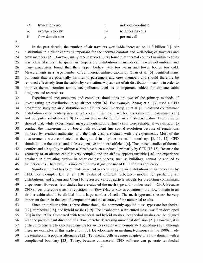
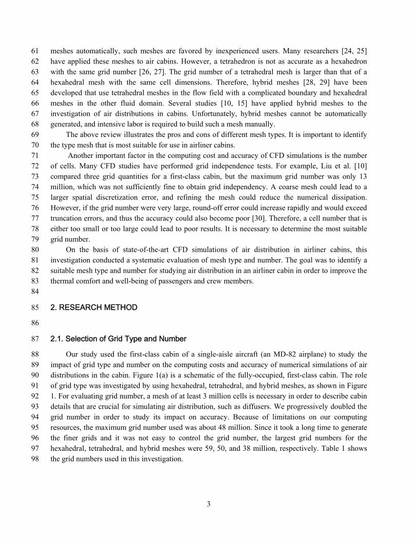
Our study used the first-class cabin of a single-aisle aircraft (an MD-82 airplane) to study the 88 impact of grid type and number on the computing costs and accuracy of numerical simulations of air 89 distributions in the cabin. Figure 1(a) is a schematic of the fully-occupied, first-class cabin. The role 90 of grid type was investigated by using hexahedral, tetrahedral, and hybrid meshes, as shown in Figure 91 1. For evaluating grid number, a mesh of at least 3 million cells is necessary in order to describe cabin 92 details that are crucial for simulating air distribution, such as diffusers. We progressively doubled the 93 grid number in order to study its impact on accuracy. Because of limitations on our computing 94 resources, the maximum grid number used was about 48 million. Since it took a long time to generate 95 the finer grids and it was not easy to control the grid number, the largest grid numbers for the 96 hexahedral, tetrahedral, and hybrid meshes were 59, 50, and 38 million, respectively. Table 1 shows 97 the grid numbers used in this investigation. 98

4

99

(a) (b) 100

101

(c) (d) 102 Figure 1. (a) Schematic of the fully-occupied, first-class cabin; and mesh distribution at the back 103

section for different mesh grid types: (b) hexahedral mesh, (c) tetrahedral mesh, and (d) hybrid mesh 104 with 24 million cells. 105

106 Table 1. Grid numbers, dimensions, and Y+ values used in this study 107

Mesh type AbbreviationCell number

(millions) Global mesh

size (mm) Surface-average

Y+

Hybrid

HY3 3 64 5.02

HY6 6 48 3.84

HY12 12 32 3.32

HY24 24 24 2.86

HY38 38 24 2.21

Tetrahedral

T3 3 80 4.38 T6 6 64 3.33

T12 12 48 2.45 T24 24 32 2.04 T50 50 24 1.67

Hexahedral

H12 12 24 2.11 H24 24 24 1.89

H59 59 24 1.54

108 109 110

5

Figure 1 shows the grid distributions of the three mesh types. Different mesh types had similar 111 mesh distributions. For example, the mesh was very fine in the regions close to the walls, manikins, 112 and air diffusers because of large gradients in the variables, while coarse meshes were used in the 113 main flow region. This investigation defined the large mesh dimension used in the main flow region 114 as the global mesh dimension. For the hexahedral mesh, as depicted in Figure 1(b), the distribution of 115 the meshes was uniform in most of the main flow region. Because the diffuser size was only 3 mm 116 and the global mesh dimension was much larger than that, we gradually increased the mesh dimension 117 for the diffusers to the main flow to ensure grid quality. Figure 1(c) shows the tetrahedral mesh 118 distribution and Figure 1(d) the hybrid mesh distribution, under the same strategy as that used for the 119 hexahedral meshes. The hybrid mesh was divided into three flow regions: the region with regular 120 geometry close to the aisle and floor, where hexahedral meshes were used; the region with irregular 121 geometry close to the diffusers, walls, ceiling, seats, and manikins, where tetrahedral meshes were 122 used; and the transition regions, where pyramidal meshes were used. 123 124

2.2. Turbulence models and numerical scheme 125

126 CFD simulations of air distributions in airliner cabins would need to use turbulence models, as 127

current computer capacity and speed are insufficient to simulate the details of turbulence flow in 128 airliner cabin. Among various turbulence models, Liu et al. [10] recommended large-eddy-simulations 129 (LES) and detached-eddy-simulations (DES) for airflow simulations in airliner cabins. However, these 130 models require long a computing time and high mesh density. Zhang et al. [31] concluded that the 131 LES model provided the most detailed flow features, while the v2f and re-normalization (RNG) k-ε 132 models could produce acceptable results with greatly reduced computing time. Since the RNG k-ε 133 model is one of the most popular turbulence models used in design practice, the current study used 134 this model to simulate cabin flows. Because the airflow in an airliner cabin can be transitional, this 135 study also simulated the flow as transient or unsteady. 136

The governing equations for the RNG k-ε model for both steady and transient flows can be 137 written in a general form: 138 139

,[ ]i effi i

u St t x x

(1) 140

141 where ϕ represents the flow variables (air velocity, energy, and turbulence parameters), Гϕ,eff is the 142 effective diffusion coefficient, and Sϕ is the source term. When ϕ = 1, then equation (1) becomes the 143 continuity equation. 144

This study used commercial CFD software FLUENT [32] for all numerical simulations. The 145 Navier-Stokes equation was discretized by the finite-volume method [33, 34, 35]. We employed the 146 SIMPLE algorithm to couple the pressure and velocity calculations. The PRESTO! scheme was 147 adopted for pressure discretization, and the first-order upwind scheme was used for all the other 148 variables. We tested the second-order scheme, but the calculation did not lead to a converged solution 149 [10]; this result was unfortunate, and the scheme should be further investigated in the future. This 150

6

investigation started an unsteady-state simulation that was based on the results of a steady-state 151 simulation. We estimated that the unsteady-state simulation took one time constant of 50 s to reach a 152 stable flow field. The computation then continued for another 100 s, after which time-averaged 153 simulation results could be obtained. 154

For the regions near the walls, our study used the enhanced wall function [32], which required 155 that the Y+ value be less than 30. Table 1 shows the surface-averaged wall Y+ values, which were all 156 smaller than 5; thus, the wall function could be used. 157

The study considered the solutions to be converged when the sum of the normalized residuals for 158 all the cells satisfied the conditions shown in Table 2. The normalized residuals were defined as: 159 160

(2) 161

162

where P and nb are the given variable at the present and neighboring cells, respectively; Pa is the 163

coefficient of the variable at the present cell; nba are the correlation coefficients of the variable at the 164

neighboring cells; and b is the source term or boundary conditions. 165 166

167 Table 2. Residual values below which solutions are considered to be converged, for the three different 168

mesh grid types 169

Residuals Hexahedral Tetrahedral Hybrid

continuity 10-4 10-4 10-4

velocity 10-3 10-3 10-3

energy 10-6 10-6 10-6

k 10-3 10-3 10-3

ε 10-4 10-4 10-4

170 171

 nb nb P PcellsP nb

P PcellsP

a b aR

a

7

2.3. Numerical errors 172

173 Discretizing the partial differential governing equation (Eq. 1) gives rise to three types of errors: 174

truncation errors, errors introduced by the numerical definitions of boundary conditions, and round-off 175 errors [36]. The following two sub-sections present the method we used to estimate the truncation 176 errors and round-off errors because they are related to grid type and number. 177 178

2.3.1. Truncation errors 179

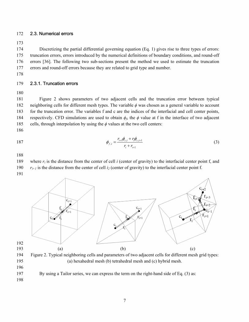
180 Figure 2 shows parameters of two adjacent cells and the truncation error between typical 181

neighboring cells for different mesh types. The variable ϕ was chosen as a general variable to account 182 for the truncation error. The variables f and c are the indices of the interfacial and cell center points, 183 respectively. CFD simulations are used to obtain ϕf, the ϕ value at f in the interface of two adjacent 184 cells, through interpolation by using the ϕ values at the two cell centers: 185 186

1 , , 1,

1

i c i i c if i

i i

r r

r r

(3) 187

188 where ri is the distance from the center of cell i (center of gravity) to the interfacial center point f, and 189 ri+1 is the distance from the center of cell i2 (center of gravity) to the interfacial center point f. 190

191

192 (a) (b) (c) 193

Figure 2. Typical neighboring cells and parameters of two adjacent cells for different mesh grid types: 194 (a) hexahedral mesh (b) tetrahedral mesh and (c) hybrid mesh. 195

196 By using a Tailor series, we can express the term on the right-hand side of Eq. (3) as: 197

198

8

2 21 +11 , , 1 1 , , 1 , , 1 , ,

1 1( ) ( ) ( ) ( ) +...

2! 2!i i i ii c i i c i i f i i f i i f i i f i i f i i f ir r r r r r r r r r r r

199

(4) 200

iir r

, 11 iir r

(5) 201

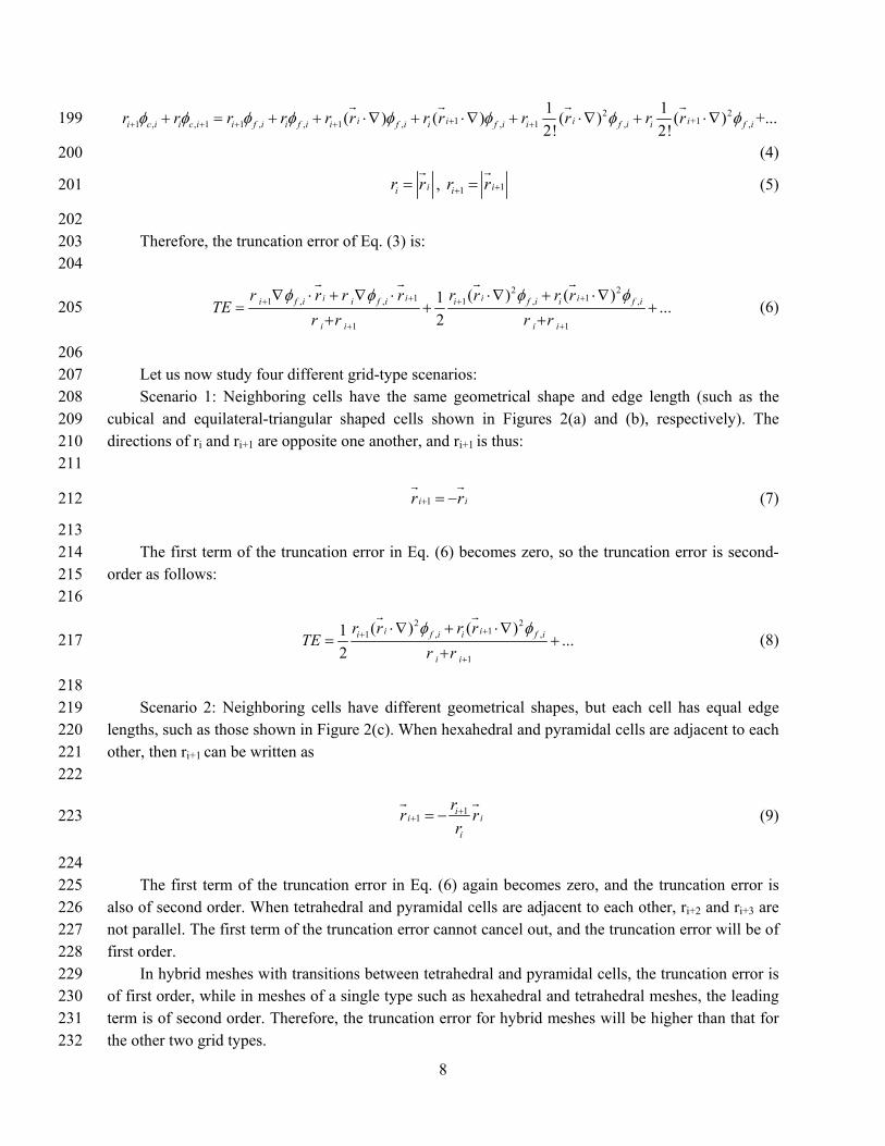
202 Therefore, the truncation error of Eq. (3) is: 203

204

2 21 11 , , 1 , ,

1 1

( ) ( )1...

2

i i i ii f i i f i i f i i f i

i i i i

r r r r r r r rTE

r r r r

(6) 205

206 Let us now study four different grid-type scenarios: 207 Scenario 1: Neighboring cells have the same geometrical shape and edge length (such as the 208

cubical and equilateral-triangular shaped cells shown in Figures 2(a) and (b), respectively). The 209 directions of ri and ri+1 are opposite one another, and ri+1 is thus: 210

211

1i ir r

(7) 212

213 The first term of the truncation error in Eq. (6) becomes zero, so the truncation error is second-214

order as follows: 215 216

2 211 , ,

1

( ) ( )1...

2

i ii f i i f i

i i

r r r rTE

r r

(8) 217

218 Scenario 2: Neighboring cells have different geometrical shapes, but each cell has equal edge 219

lengths, such as those shown in Figure 2(c). When hexahedral and pyramidal cells are adjacent to each 220 other, then ri+1 can be written as 221 222

11

ii i

i

rr r

r

(9) 223

224 The first term of the truncation error in Eq. (6) again becomes zero, and the truncation error is 225

also of second order. When tetrahedral and pyramidal cells are adjacent to each other, ri+2 and ri+3 are 226 not parallel. The first term of the truncation error cannot cancel out, and the truncation error will be of 227 first order. 228

In hybrid meshes with transitions between tetrahedral and pyramidal cells, the truncation error is 229 of first order, while in meshes of a single type such as hexahedral and tetrahedral meshes, the leading 230 term is of second order. Therefore, the truncation error for hybrid meshes will be higher than that for 231 the other two grid types. 232

9

Scenario 3: Neighboring cells have the same geometrical shape, but each cell has different edge 233 lengths (such as a rectangular parallelepiped and scalene-triangular shaped cell). The first term of the 234 errors arising on opposite hexahedral cell faces cancels out completely on the basis of Eq. (9), since 235 the cell faces are parallel. However, because the cell faces are not parallel for tetrahedral meshes, the 236 truncation error is still of first order. Hence, hexahedral meshes are superior to tetrahedral meshes 237 with a similar resolution [21]. 238

Scenario 4: Neighboring cells have different geometrical shapes, and each cell has different edge 239 lengths. The truncation error is always of first order. 240 241

Refining the meshes would reduce the truncation error. When the mesh is sufficiently fine, mesh 242 type has little influence on the accuracy of simulation results because 243 244

0lim ( ) ( ) 0ir iTE O r (10) 245

246

2.3.2. Round-off errors 247

248

Round-off error, ni , is the difference between the exact solution

ni and the approximated 249

solution n

i of the governing equation, as shown in Eq. (11). Limited computer word length would 250

lead to the round-off error. As the time step size and cell dimension decrease, the round-off error 251 increases while the truncation error decreases. Decreasing the cell dimension and time step size does 252 ensure more accurate results. When the time step size and cell dimension are very small, the accuracy 253 is compromised because the round-off error may overtake the truncation error. Therefore, the grid 254 number should be small enough to prevent round-off error. 255 256

nn nii i (11) 257

258 It is necessary to identify the relationship between numerical errors (including round-off and 259

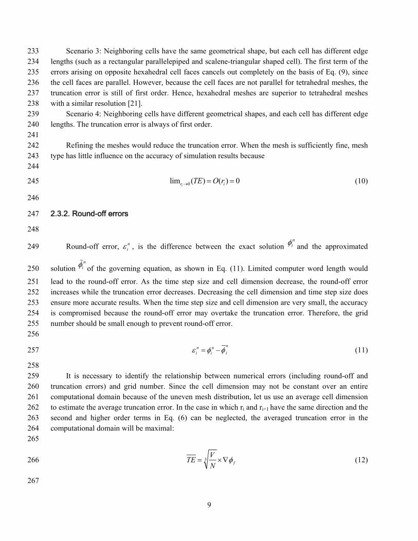
truncation errors) and grid number. Since the cell dimension may not be constant over an entire 260 computational domain because of the uneven mesh distribution, let us use an average cell dimension 261 to estimate the average truncation error. In the case in which ri and ri+1 have the same direction and the 262 second and higher order terms in Eq. (6) can be neglected, the averaged truncation error in the 263 computational domain will be maximal: 264 265

3 f

VTE

N (12) 266

267

10

where N is the grid number and V is the flow domain size (15.5 m3 for the first-class cabin). In the 268 case in which ri and ri+1 have the opposite direction and the second and higher order terms in Eq. (6) 269 can be neglected, the averaged truncation error will be zero. 270 271

For a CFD program with double precision parameters, the storage accuracy of a computer can be 272 as high as 10-15. If we iterate 20,000 time steps for a 150 s unsteady-state simulation in the first-class 273 cabin, the maximal round-off error is: 274

1520,000 /10 roE N (13) 275

276 The total numerical error is then: 277

11 32 10 f

VErr N

N (14) 278

279 A suitable grid number for achieving the minimal numerical error can be determined by equating 280

the derivative of the right-hand term of Eq. (14) to zero. By using V = 15.5 m3, we obtain 281 282

7 34=9.2 10 fN (15) 283

284 Eq. (15) shows that a suitable grid number is a function of ϕ for the air cabin. 285

286

3. RESULTS 287

288 This section first compares the simulated results from the steady- and unsteady-state RNG k-ε 289

models with the measured data, and then discusses the impact of mesh type and number on the 290 simulated results. 291

292

3.1. Steady- and unsteady-state turbulent flow modeling 293

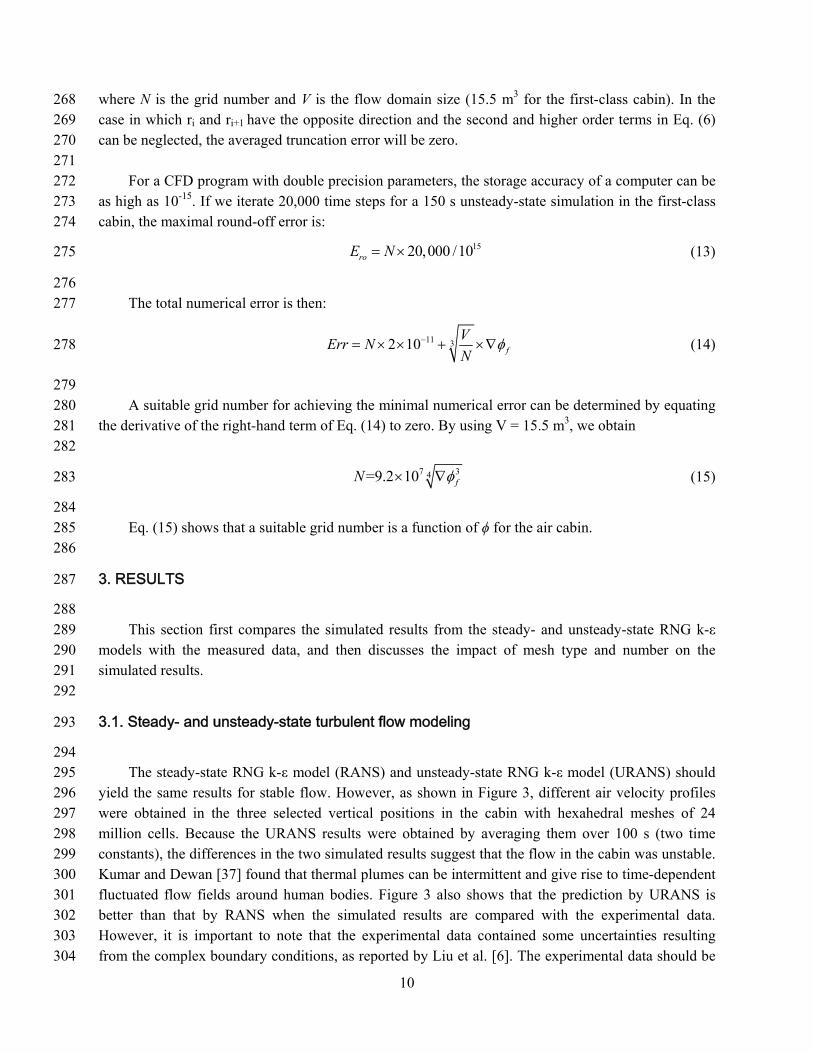
294 The steady-state RNG k-ε model (RANS) and unsteady-state RNG k-ε model (URANS) should 295

yield the same results for stable flow. However, as shown in Figure 3, different air velocity profiles 296 were obtained in the three selected vertical positions in the cabin with hexahedral meshes of 24 297 million cells. Because the URANS results were obtained by averaging them over 100 s (two time 298 constants), the differences in the two simulated results suggest that the flow in the cabin was unstable. 299 Kumar and Dewan [37] found that thermal plumes can be intermittent and give rise to time-dependent 300 fluctuated flow fields around human bodies. Figure 3 also shows that the prediction by URANS is 301 better than that by RANS when the simulated results are compared with the experimental data. 302 However, it is important to note that the experimental data contained some uncertainties resulting 303 from the complex boundary conditions, as reported by Liu et al. [6]. The experimental data should be 304

11

used only as a reference, rather than a criterion. Because of the unstable flow features, this 305 investigation used URANS to study the impact of grid type and number on the prediction of air 306 distributions in the airliner cabin. 307 308

309

310

311

Figure 3. Comparison of the simulated air velocity profiles obtained by the RNG k-ε and unsteady-312 state RNG k-ε models with those measured in the occupied first-class cabin. 313

314

3.2. Impact of grid number on the simulated results 315

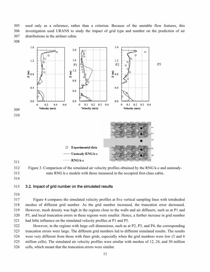
316 Figure 4 compares the simulated velocity profiles at five vertical sampling lines with tetrahedral 317

meshes of different grid number. As the grid number increased, the truncation error decreased. 318 However, mesh density was high in the regions close to the walls and air diffusers, such as at P1 and 319 P5, and local truncation errors in these regions were smaller. Hence, a further increase in grid number 320 had little influence on the simulated velocity profiles at P1 and P5. 321

However, in the regions with large cell dimensions, such as at P2, P3, and P4, the corresponding 322 truncation errors were large. The different grid numbers led to different simulated results. The results 323 were very different from those with finer grids, especially when the grid numbers were low (3 and 6 324 million cells). The simulated air velocity profiles were similar with meshes of 12, 24, and 50 million 325 cells, which meant that the truncation errors were similar. 326

P1 P2 P5

12

Figure 4 also shows the measured air velocity profiles at the five vertical positions. The 327 simulated and measured results show similar trends. The differences between the two results can be 328 attributed to numerical errors and experimental uncertainties. 329

330

331

332 Figure 4. Comparison of the vertical air velocity profiles computed using different tetrahedral meshes 333

with the experimental data at the five locations in the occupied cabin. 334 335

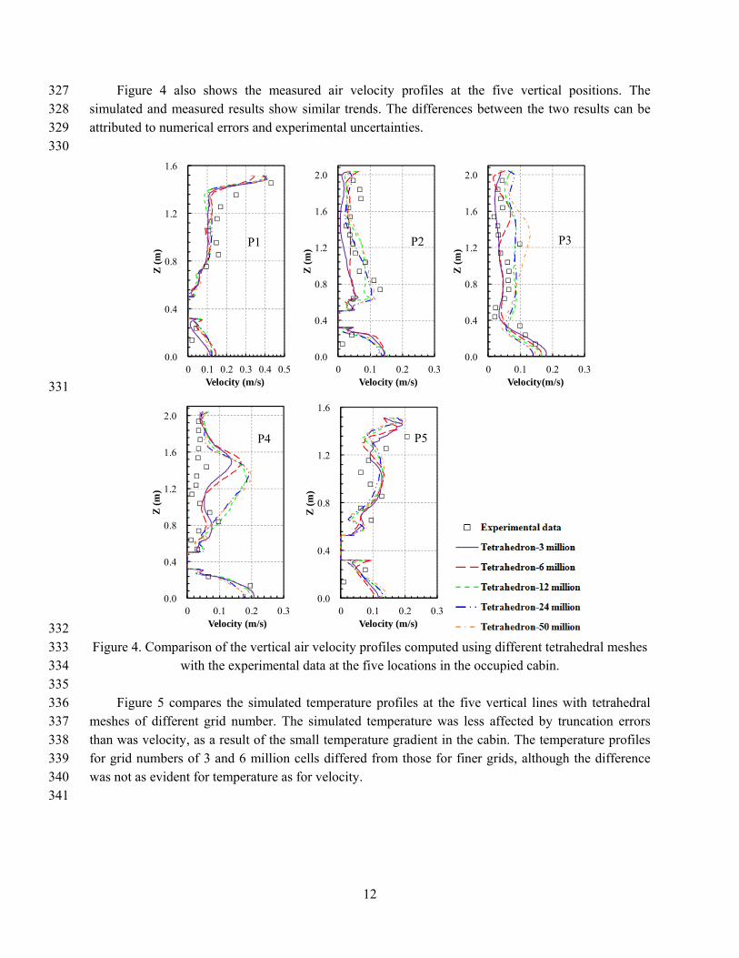
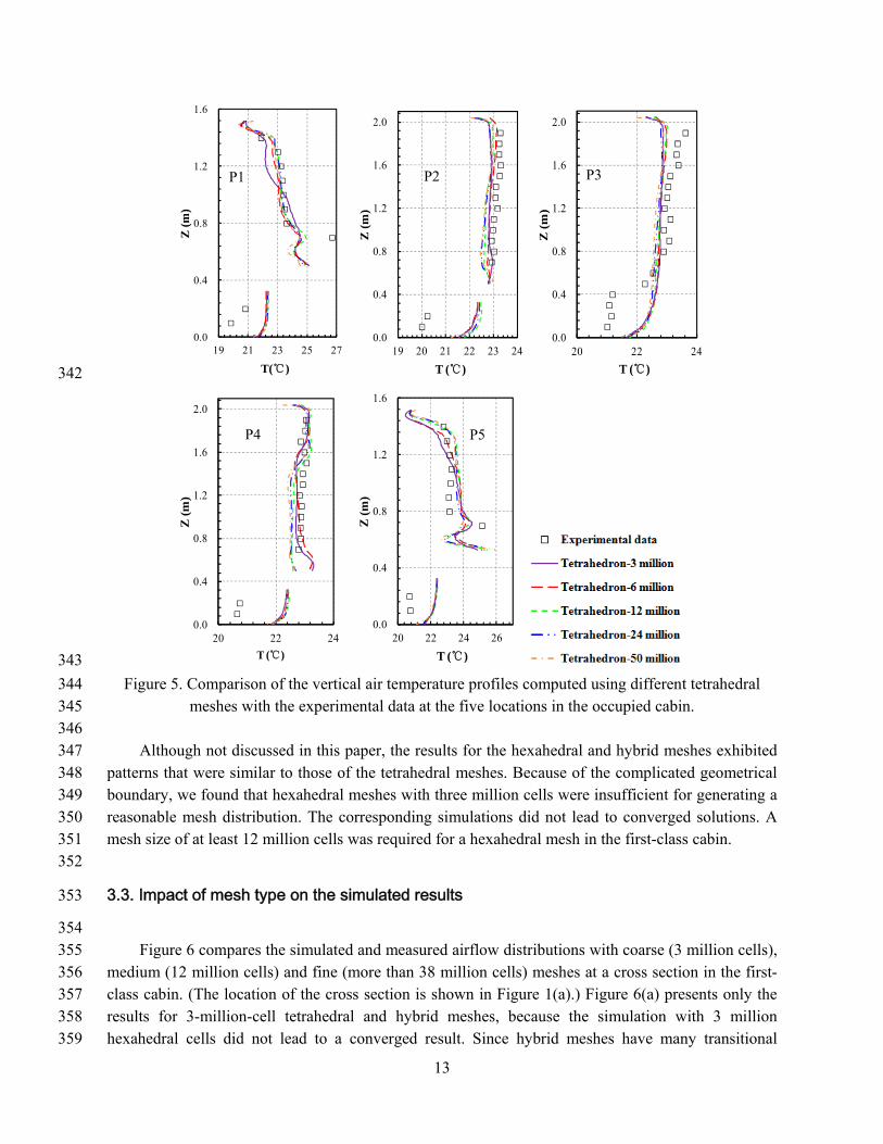
Figure 5 compares the simulated temperature profiles at the five vertical lines with tetrahedral 336 meshes of different grid number. The simulated temperature was less affected by truncation errors 337 than was velocity, as a result of the small temperature gradient in the cabin. The temperature profiles 338 for grid numbers of 3 and 6 million cells differed from those for finer grids, although the difference 339 was not as evident for temperature as for velocity. 340 341

0.0

0.4

0.8

1.2

1.6

0 0.1 0.2 0.3 0.4 0.5

Z (

m)

Velocity (m/s)

0.0

0.4

0.8

1.2

1.6

2.0

0 0.1 0.2 0.3

Z (

m)

Velocity (m/s)

0.0

0.4

0.8

1.2

1.6

2.0

0 0.1 0.2 0.3

Z (

m)

Velocity(m/s)

0.0

0.4

0.8

1.2

1.6

2.0

0 0.1 0.2 0.3

Z (

m)

Velocity (m/s)

0.0

0.4

0.8

1.2

1.6

0 0.1 0.2 0.3

Z (

m)

Velocity (m/s)

P1 P2 P3

P4 P5

13

342

343

Figure 5. Comparison of the vertical air temperature profiles computed using different tetrahedral 344 meshes with the experimental data at the five locations in the occupied cabin. 345

346 Although not discussed in this paper, the results for the hexahedral and hybrid meshes exhibited 347

patterns that were similar to those of the tetrahedral meshes. Because of the complicated geometrical 348 boundary, we found that hexahedral meshes with three million cells were insufficient for generating a 349 reasonable mesh distribution. The corresponding simulations did not lead to converged solutions. A 350 mesh size of at least 12 million cells was required for a hexahedral mesh in the first-class cabin. 351 352

3.3. Impact of mesh type on the simulated results 353

354 Figure 6 compares the simulated and measured airflow distributions with coarse (3 million cells), 355

medium (12 million cells) and fine (more than 38 million cells) meshes at a cross section in the first-356 class cabin. (The location of the cross section is shown in Figure 1(a).) Figure 6(a) presents only the 357 results for 3-million-cell tetrahedral and hybrid meshes, because the simulation with 3 million 358 hexahedral cells did not lead to a converged result. Since hybrid meshes have many transitional 359

0.0

0.4

0.8

1.2

1.6

19 21 23 25 27

Z (

m)

T(℃)

0.0

0.4

0.8

1.2

1.6

2.0

19 20 21 22 23 24Z

(m

)T (℃)

0.0

0.4

0.8

1.2

1.6

2.0

20 22 24

Z (

m)

T (℃)

0.0

0.4

0.8

1.2

1.6

2.0

20 22 24

Z (

m)

T (℃)

0.0

0.4

0.8

1.2

1.6

20 22 24 26

Z (

m)

T (℃)

P1 P2 P3

P4 P5

14

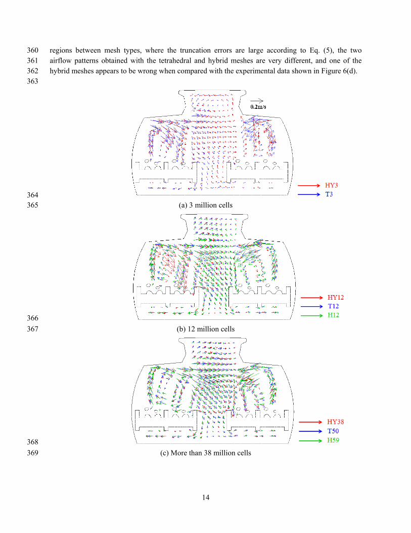
regions between mesh types, where the truncation errors are large according to Eq. (5), the two 360 airflow patterns obtained with the tetrahedral and hybrid meshes are very different, and one of the 361 hybrid meshes appears to be wrong when compared with the experimental data shown in Figure 6(d). 362

363

364 (a) 3 million cells 365

366

(b) 12 million cells 367

368

(c) More than 38 million cells 369

15

370

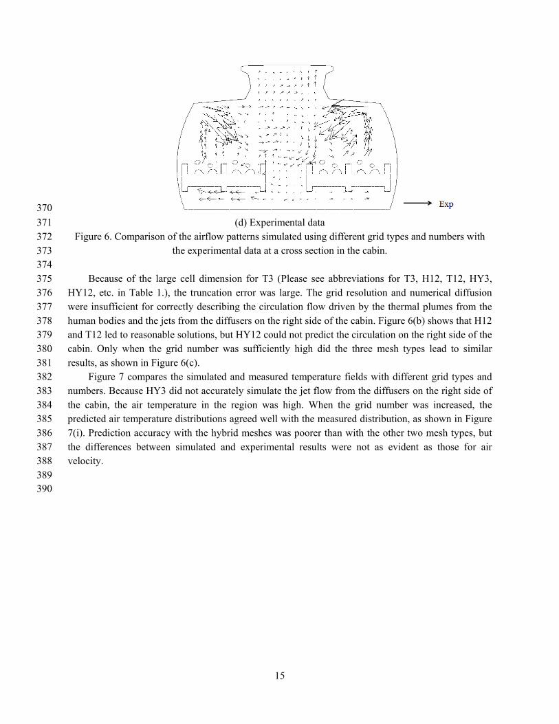
(d) Experimental data 371 Figure 6. Comparison of the airflow patterns simulated using different grid types and numbers with 372

the experimental data at a cross section in the cabin. 373 374

Because of the large cell dimension for T3 (Please see abbreviations for T3, H12, T12, HY3, 375 HY12, etc. in Table 1.), the truncation error was large. The grid resolution and numerical diffusion 376 were insufficient for correctly describing the circulation flow driven by the thermal plumes from the 377 human bodies and the jets from the diffusers on the right side of the cabin. Figure 6(b) shows that H12 378 and T12 led to reasonable solutions, but HY12 could not predict the circulation on the right side of the 379 cabin. Only when the grid number was sufficiently high did the three mesh types lead to similar 380 results, as shown in Figure 6(c). 381

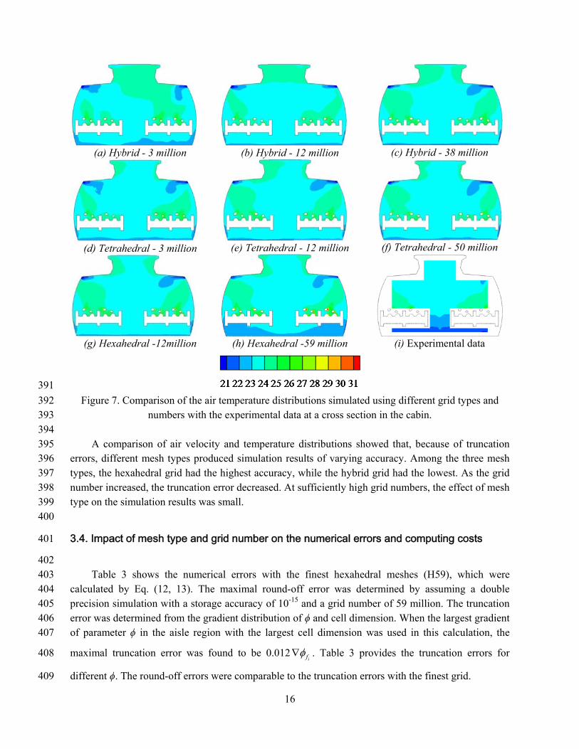
Figure 7 compares the simulated and measured temperature fields with different grid types and 382 numbers. Because HY3 did not accurately simulate the jet flow from the diffusers on the right side of 383 the cabin, the air temperature in the region was high. When the grid number was increased, the 384 predicted air temperature distributions agreed well with the measured distribution, as shown in Figure 385 7(i). Prediction accuracy with the hybrid meshes was poorer than with the other two mesh types, but 386 the differences between simulated and experimental results were not as evident as those for air 387 velocity. 388 389 390

16

(a) Hybrid - 3 million

(b) Hybrid - 12 million

(c) Hybrid - 38 million

(d) Tetrahedral - 3 million

(e) Tetrahedral - 12 million

(f) Tetrahedral - 50 million

(g) Hexahedral -12million

(h) Hexahedral -59 million

(i) Experimental data

391

Figure 7. Comparison of the air temperature distributions simulated using different grid types and 392 numbers with the experimental data at a cross section in the cabin. 393

394 A comparison of air velocity and temperature distributions showed that, because of truncation 395

errors, different mesh types produced simulation results of varying accuracy. Among the three mesh 396 types, the hexahedral grid had the highest accuracy, while the hybrid grid had the lowest. As the grid 397 number increased, the truncation error decreased. At sufficiently high grid numbers, the effect of mesh 398 type on the simulation results was small. 399 400

3.4. Impact of mesh type and grid number on the numerical errors and computing costs 401

402 Table 3 shows the numerical errors with the finest hexahedral meshes (H59), which were 403

calculated by Eq. (12, 13). The maximal round-off error was determined by assuming a double 404 precision simulation with a storage accuracy of 10-15 and a grid number of 59 million. The truncation 405 error was determined from the gradient distribution of ϕ and cell dimension. When the largest gradient 406 of parameter ϕ in the aisle region with the largest cell dimension was used in this calculation, the 407

maximal truncation error was found to be 0.012if

. Table 3 provides the truncation errors for 408

different ϕ. The round-off errors were comparable to the truncation errors with the finest grid. 409

17

410 411

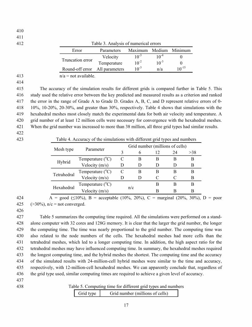
Table 3. Analysis of numerical errors 412

Error Parameters Maximum Medium Minimum

Truncation error Velocity 10-3 10-4 0

Temperature 10-2 10-3 0 Round-off error All parameters 10-3 n/a 10-15

n/a = not available. 413 414

The accuracy of the simulation results for different grids is compared further in Table 5. This 415 study used the relative error between the key predicted and measured results as a criterion and ranked 416 the error in the range of Grade A to Grade D. Grades A, B, C, and D represent relative errors of 0-417 10%, 10-20%, 20-30%, and greater than 30%, respectively. Table 4 shows that simulations with the 418 hexahedral meshes most closely match the experimental data for both air velocity and temperature. A 419 grid number of at least 12 million cells were necessary for convergence with the hexahedral meshes. 420 When the grid number was increased to more than 38 million, all three grid types had similar results. 421 422

Table 4. Accuracy of the simulations with different grid types and numbers 423

Mesh type Parameter Grid number (millions of cells)

3 6 12 24 >38

Hybrid Temperature (oC) C B B B B

Velocity (m/s) D D D D B

Tetrahedral Temperature (oC) C B B B B

Velocity (m/s) D D C C B

Hexahedral Temperature (oC)

n/c B B B

Velocity (m/s) B B B

A = good (≤10%), B = acceptable (10%, 20%), C = marginal (20%, 30%), D = poor 424 (>30%), n/c = not converged. 425

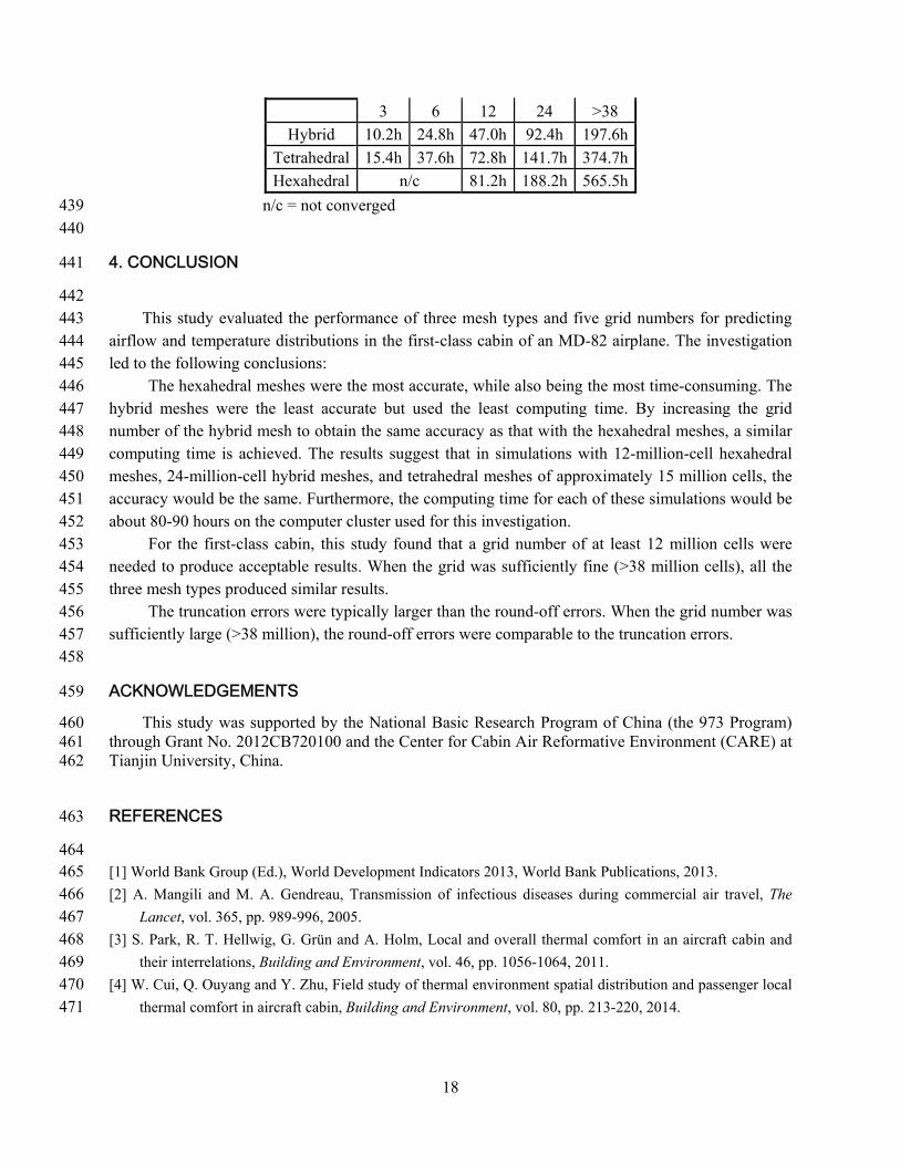
426 Table 5 summarizes the computing time required. All the simulations were performed on a stand-427

alone computer with 32 cores and 128G memory. It is clear that the larger the grid number, the longer 428 the computing time. The time was nearly proportional to the grid number. The computing time was 429 also related to the node numbers of the cells. The hexahedral meshes had more cells than the 430 tetrahedral meshes, which led to a longer computing time. In addition, the high aspect ratio for the 431 tetrahedral meshes may have influenced computing time. In summary, the hexahedral meshes required 432 the longest computing time, and the hybrid meshes the shortest. The computing time and the accuracy 433 of the simulated results with 24-million-cell hybrid meshes were similar to the time and accuracy, 434 respectively, with 12-million-cell hexahedral meshes. We can apparently conclude that, regardless of 435 the grid type used, similar computing times are required to achieve a given level of accuracy. 436 437

Table 5. Computing time for different grid types and numbers 438

Grid type Grid number (millions of cells)

18

3 6 12 24 >38

Hybrid 10.2h 24.8h 47.0h 92.4h 197.6h

Tetrahedral 15.4h 37.6h 72.8h 141.7h 374.7h

Hexahedral n/c 81.2h 188.2h 565.5h

n/c = not converged 439 440

4. CONCLUSION 441

442 This study evaluated the performance of three mesh types and five grid numbers for predicting 443

airflow and temperature distributions in the first-class cabin of an MD-82 airplane. The investigation 444 led to the following conclusions: 445

The hexahedral meshes were the most accurate, while also being the most time-consuming. The 446 hybrid meshes were the least accurate but used the least computing time. By increasing the grid 447 number of the hybrid mesh to obtain the same accuracy as that with the hexahedral meshes, a similar 448 computing time is achieved. The results suggest that in simulations with 12-million-cell hexahedral 449 meshes, 24-million-cell hybrid meshes, and tetrahedral meshes of approximately 15 million cells, the 450 accuracy would be the same. Furthermore, the computing time for each of these simulations would be 451 about 80-90 hours on the computer cluster used for this investigation. 452

For the first-class cabin, this study found that a grid number of at least 12 million cells were 453 needed to produce acceptable results. When the grid was sufficiently fine (>38 million cells), all the 454 three mesh types produced similar results. 455

The truncation errors were typically larger than the round-off errors. When the grid number was 456 sufficiently large (>38 million), the round-off errors were comparable to the truncation errors. 457 458

ACKNOWLEDGEMENTS 459

This study was supported by the National Basic Research Program of China (the 973 Program) 460 through Grant No. 2012CB720100 and the Center for Cabin Air Reformative Environment (CARE) at 461 Tianjin University, China. 462

REFERENCES 463

464 [1] World Bank Group (Ed.), World Development Indicators 2013, World Bank Publications, 2013. 465 [2] A. Mangili and M. A. Gendreau, Transmission of infectious diseases during commercial air travel, The 466

Lancet, vol. 365, pp. 989-996, 2005. 467 [3] S. Park, R. T. Hellwig, G. Grün and A. Holm, Local and overall thermal comfort in an aircraft cabin and 468

their interrelations, Building and Environment, vol. 46, pp. 1056-1064, 2011. 469 [4] W. Cui, Q. Ouyang and Y. Zhu, Field study of thermal environment spatial distribution and passenger local 470

thermal comfort in aircraft cabin, Building and Environment, vol. 80, pp. 213-220, 2014. 471

19

[5] J. Guan, C. Wang, K. Gao, X. Yang, C. H. Lin and C. Lu, Measurements of volatile organic compounds in 472 aircraft cabins. Part II: Target list, concentration levels and possible influencing factors, Building and 473 Environment, vol. 75, pp. 170-175, 2014. 474

[6] W. Liu, S. Mazumdar, Z. Zhang, S. B. Poussou, J. Liu, C. H. Lin and Q. Chen, State-of-the-art methods for 475 studying air distributions in commercial airliner cabins, Building and Environment, vol. 47, pp. 5-12, 2012. 476

[7] Z. Zhang, X. Chen, S. Mazumdar, T. Zhang and Q. Chen, Experimental and numerical investigation of 477 airflow and contaminant transport in an airliner cabin mockup, Building and Environment, vol. 44, pp. 85-478 94, 2009. 479

[8] F. Li, J. Liu, J. Pei, C. H. Lin and Q. Chen, Experimental study of gaseous and particulate contaminants 480 distribution in an aircraft cabin, Atmospheric Environment, vol. 85, pp. 223-233, 2014. 481

[9] W. Liu, J. Wen, J. Chao, W. Yin, C. Shen, D. Lai, C. H. Lin, J. Liu, H. Sun and Q. Chen, Accurate and 482 high-resolution boundary conditions and flow fields in the first-class cabin of an MD-82 commercial 483 airliner, Atmospheric Environment, vol. 56, pp. 33-44, 2012. 484

[10] W. Liu, J. Wen, C. H. Lin, J. Liu, Z. Long and Q. Chen, Evaluation of various categories of turbulence 485 models for predicting air distribution in an airliner cabin, Building and Environment, vol. 65, pp. 118-131, 486 2013. 487

[11] T. T. Zhang, P. Li and S. Wang, A personal air distribution system with air terminals embedded in chair 488 armrests on commercial airplanes, Building and Environment, vol. 47, pp. 89-99, 2012. 489

[12] A. Wang, Y. Zhang, Y. Sun and X. Wang, Experimental study of ventilation effectiveness and air velocity 490 distribution in an aircraft cabin mockup, Building and Environment, vol. 43, pp. 337-343, 2008. 491

[13] M. Wang, C. H. Lin and Q. Chen, Determination of particle deposition in enclosed spaces by Detached 492 Eddy Simulation with the Lagrangian method, Atmospheric Environment, vol. 45, pp. 5376-5384, 2011. 493

[14] C. Chen, W. Liu, F. Li, C. H. Lin, J. Liu, J. Pei and Q. Chen, A hybrid model for investigating transient 494 particle transport in enclosed environments, Building and Environment, vol. 62, pp. 45-54, 2013. 495

[15] S. Liu, L. Xu, J. Chao, C. Shen, J. Liu, H. Sun, X. Xiao and G. Nan, Thermal environment around 496 passengers in an aircraft cabin, HVAC&R Res., vol. 19, pp. 627-634, 2013. 497

[16] Z. Zhang and Q. Chen, Comparison of the Eulerian and Lagrangian methods for predicting particle 498 transport in enclosed spaces, Atmospheric Environment, vol. 41, pp. 5236-5248, 2007. 499

[17] J. M. A. Hofman, Control-fluid interaction in air-conditioned aircraft cabins: A demonstration of stability 500 analysis for partitioned dynamical systems, Comput. Meth. Appl. Mech. Eng., vol. 192, pp. 4947-4963, 501 2003. 502

[18] T. Zhang and Q. Chen, Novel air distribution systems for commercial aircraft cabins, Building and 503 Environment, vol. 42, pp. 1675-1684, 2007. 504

[19] W. Liu, C. H. Lin, J. Liu and Q. Chen, Simplifying geometry of an airliner cabin for CFD simulations, 505 Indoor Air Quality and Climate 2011: Proc. 12th Int. Indoor Air Quality and Climate Conf., Austin, Texas, 506 2011. 507

[20] J. F. Thompson, F. C. Thames, C. W. Mastin, Automatic numerical generation of body-fitted curvilinear 508 coordinates for a field containing any number of arbitrary 2-D bodies, J. Comput. Phys., vol. 15, pp. 299-509 319, 1974. 510

[21] M. M. Hefny and R. Ooka, CFD analysis of pollutant dispersion around buildings: Effect of cell geometry. 511 Building and Environment, vol. 44, pp. 1699-1706, 2009. 512

[22] R. Löhner, K. Morgan, J. Peraire and M. Vahdati, Finite element flux-corrected transport (FEM-FCT) for 513 the Euler and Navier-Stokes equations, Int. J. Numer., vol. 7, pp. 1093-1109, 1987. 514

20

[23] A. Jameson and T. J. Baker, Improvements to the aircraft Euler method, AIAA-87-0425, 1987. 515 [24] V. Bianco, O. Manca, S. Nardini and M. Roma, Numerical investigation of transient thermal and 516

fluidynamic fields in an executive aircraft cabin, Appl. Therm. Eng., vol. 29, pp. 3418-3425, 2009. 517 [25] S. S. Isukapalli, S. Mazumdar, P. George, B. Wei, B. Jones and C. P. Weisel, Computational fluid 518

dynamics modeling of transport and deposition of pesticides in an aircraft cabin, Atmospheric 519 Environment, vol. 68, pp. 198-207, 2013. 520

[26] G. Yu, B. Yu, S. Sun, and W. Q. Tao, Comparative study on triangular and quadrilateral meshes by a 521 finite-volume method with a central difference scheme, Numer. Heat Transfer B, vol. 62, pp. 243-263, 522 2012. 523

[27] F. Juretic´ and A. D. Gosman, Error analysis of the finite-volume method with respect to mesh type, 524 Numer. Heat Transfer B, vol. 57, pp. 414-439, 2010. 525

[28] Y. Kallinderis, A. Khawaja and H. McMorris, Hybrid prismatic/tetrahedral grid generation for viscous 526 flows around complex geometries. AIAA J., vol. 34, pp. 291-298, 1996. 527

[29] Tysell, L, Hybrid grid generation for complex 3D geometries, Numerical Grid Generation in 528 Computational Field Simulations 2000: Proc. 7th Int. Numerical Grid Generation in Computational Field 529 Simulations Conf., Whistler, pp. 337-346, British Columbia, Canada, 2000. 530

[30] J. Tu, G. H. Yeoh and C. Liu, Computational Fluid Dynamics: A Practical Approach, pp. 147-148, 531 Butterworth-Heinemann, Oxford, 2007. 532

[31] Z. Zhang, W. Zhang, Z. Zhai and Q. Chen, Evaluation of various turbulence models in predicting airflow 533 and turbulence in enclosed environments by CFD: Part 2-Comparison with experimental data from 534 literature, HVAC&R Res., vol. 13, pp. 853-870, 2007. 535

[32] ANSYS, ANSYS Fluent 13.0 Documentation, ANSYS, Inc., Lebanon, NH, 2010. 536 [33] S. R. Mathur and J. Y. Murthuy, A pressure-based method for unstructured meshes, Numer. Heat Transfer 537

B, vol. 31, pp. 195-215, 1997. 538 [34] L. Sun, S. R. Mathur, and J. Y. Murthy, An unstructured finite-volume method for incompressible flows 539

with complex immersed boundaries, Numer. Heat Transfer B, vol. 58, pp. 217-241, 2010. 540 [35] A. Dalal, V. Eswaran, and G. Biswas, A finite-volume method for Navier-Stokes equations on 541

unstructured meshes, Numer. Heat Transfer B, vol. 53, pp. 238-259, 2008. 542 [36] P. V. Nielsen, Flow in air-conditioned rooms, Ph.D. thesis, Technical University of Denmark, Lyngby, 543

Denmark, 1976. 544 [37] R. Kumar and A. Dewan, URANS computations with buoyancy corrected turbulence models for turbulent 545

thermal plume, Int. J. Heat Mass Transfer, vol. 72, pp. 680-689, 2014. 546 547