Mesoscopic full counting statistics and exclusion models

Eur. Phys. J. B 43, 529–541 (2005)DOI: 10.1140/epjb/e2005-00087-5 THE EUROPEAN

PHYSICAL JOURNAL B

Mesoscopic full counting statistics and exclusion models

P.-E. Roche1,2,a, B. Derrida3, and B. Doucot4

1 Centre de Recherches sur les Tres Basses Temperatures, Laboratoire du CNRS, associe a l’Universite Joseph Fourier,25 avenue des Martyrs, 38042 Grenoble Cedex 9, France

2 Laboratoire Pierre Aigrain, Ecole Normale Superieure, 24 rue Lhomond, 75231 Paris Cedex 05, France3 Laboratoire de Physique Statistique, Ecole Normale Superieure, 24 rue Lhomond, 75231 Paris Cedex 05, France4 Laboratoire de Physique Theorique et des Hautes Energies, Universite Denis Diderot, 4 place Jussieu,

75252 Paris Cedex 05, France

Received 23 December 2003 / Received in final form 6 December 2004Published online 30 March 2005 – c© EDP Sciences, Societa Italiana di Fisica, Springer-Verlag 2005

Abstract. We calculate the distribution of current fluctuations in two simple exclusion models. Althoughthese models are classical, we recover even for small systems such as a simple or a double barrier, thesame distibution of current as given by traditional formalisms for quantum mesoscopic conductors. Dueto their simplicity, the full counting statistics in exclusion models can be reduced to the calculation of thelargest eigenvalue of a matrix, the size of which is the number of internal configurations of the system. Asexamples, we derive the shot noise power and higher order statistics of current fluctuations (skewness, fullcounting statistics, ....) of various conductors, including multiple barriers, diffusive islands between tunnelbarriers and diffusive media. A special attention is dedicated to the third cumulant, which experimentalmeasurability has been demonstrated lately.

PACS. 05.40.-a Fluctuation phenomena, random processes, noise, and Brownian motion –73.23.-bElectronic transport in mesoscopic systems – 72.70.+m Noise processes and phenomena

1 Introduction

A constant voltage difference across a conductor drives anelectrical current which will always fluctuate around itsmean value. Fluctuations result from random microscopicprocesses (thermal relaxation, scattering, tunneling...) un-dergone by the charge carriers. These fluctuations can beconsidered as an undesirable noise but also as a rich sig-nature of the basic transport mechanisms occurring inthe conductor. This second perspective has concentratedmuch attention in the mesoscopic community over the lastdecade [1].

In our previous paper [2] we gave evidence that thestatistics of current fluctuations in a large classical model,the symmetric exclusion process, are identical to the onesderived for quantum mesoscopic conductors [3]. Here, weshow that exclusion models allow also to recover the cur-rent fluctuations of small systems such as a single or adouble barrier.

In the present paper, we develop a classical approach toderive the statistics of current fluctuations in mesoscopicconductors (“quantum conductors”) and more generallyin conductors smaller than the electronic inelastic meanfree path and for some inelastic conductors. Solving thecurrent statistics problem is reduced to finding the largest

a e-mail: [email protected]

eigenvalue of a modified evolution matrix, later called thecounting matrix. We extend the well known current statis-tics for a few mesoscopic systems. Our description is basedon the exclusion process models, which have been widelystudied in statistical physics and probability theory [4–6].The main benefits of this approach are its conceptual andanalytical simplicity.

In the remaining part of this introduction section, webriefly recall the traditional approaches for mesoscopictransport (Sect. 1.1) and the basic mathematical toolsnecessary to describe current fluctuations (1.2). Section 2presents two exclusion models fitted for condensed mat-ter conductors and the procedure to derive the completestatistics of current fluctuations (later called “Full Count-ing Statistics” or FCS). In Section 3, our exclusion modelsare used to derive the current statistics of various elemen-tary conductors.

1.1 Traditional formalisms for transport in condensedmatter physics

A number of approaches have already been used to de-scribe the FCS in mesoscopic conductors. The ScatteringMatrix theory [3,7–13] is well adapted to the modelingof quantum-mechanically coherent conductors in a regimewhere electron interaction effects are sufficiently weak tobe neglected. With this strong assumption, this allows to

530 The European Physical Journal B

treat an arbitrary large number of transverse conductionchannels, which yield independent contributions to thecurrent statistics. This approach, combined with resultsfrom random matrix theory for scattering matrices [14]has lead to precise predictions for the FCS of a disorderedconductor in the diffusive regime [15]. A more direct mi-croscopic treatment of disordered systems relies on theKeldysh technique [16] to construct the non-equilibriumdensity matrix of the steady state at finite current. Disor-der averaging is then performed using a non-linear Sigmamodel representation [17]. A rather general circuit theoryhas been constructed to account for the influence of an ar-bitrary environment, described in terms of an equivalentcircuit, on the measured fluctuations of a mesoscopic con-ductor [18,19]. Semi-classical descriptions, based on theBoltzmann-Langevin model [20,21] have also been used toderive the first four cumulants of current fluctuations in adiffusive medium [22,23]. Other semi-classical approachesfocused on high order statistics and FCS of a double tunnelbarrier [24], chaotic cavities [25] and diffusive media [2,26].The semi-classical results are the same as the ones ob-tained with the corresponding quantum conductor model.

The exclusion models discussed in this paper repre-sent an extreme semi-classical approximation : the onlyquantum rule which is preserved is the Pauli exclusionprinciple. In particular, electrons have no phase and donot interfere.

1.2 Mathematical formalism for current fluctuations

If qt is the algebraic charge which flows across a sectionduring time t, the fluctuations of current I = qt/t dependsin principle on the duration t chosen to measure I. In prac-tice the long time response of the measuring electronicsapparatus sets a lower bound on t: this bound is most of-ten decades larger than all the physical times experiencedby charge carriers (diffusion time, dwell time, coherencetimes in the conductor and in the electrodes,...). Thus,experiments correspond to the t → ∞ limit, often calledthe zero-frequency limit in the shot noise literature. Inthis limit, the choice of the cross-section is irrelevant sincethe maximum charge accumulation between two differentcross-sections is finite, at least in a conductor connectedto two electrodes only.

In a conductor smaller than the inelastic mean freepath, carriers do not undergo inelastic collisions. It istherefore reasonable in many situations to neglect inter-action effects on such small length scales. Equivalently,we may then assume that these charge carriers remainon independent energy levels [1]. Consequently the statis-tics of the total current will consist in a summation ofindependent random variables corresponding to differentenergy levels. In the following, to keep equations free ofelementary-charge prefactors, we focus on carriers count-ing rather than charge counting. In addition, we will callthis generic charge carrier an electron.

If Pt,ε(Q) is the probability that Q electrons have beentransfered at the energy level ε during a time interval t,one can fully characterize the counting statistics by the

cumulant generating function:

St,ε(z) = ln

∞∑

Q=−∞Pt,ε(Q) zQ

= ln(zQ) (1)

or equivalently by cumulants (the nth order one is writtenhere):

Cn(t, ε) =∂nSt,ε(z)∂(ln z)n

(2)

we have in particular: C1 = Q, C2 = (Q − Q)2, C3 =

(Q − Q)3, C4(ε) = (Q − Q)4 − 3(Q − Q)22, ...

For a given conductor, the current at an energy level εonly depends on the boundary conditions, that is thefillings ρ

L(ε) and ρ

R(ε) of the left and right electrodes

(or “reservoirs”) at both ends of the conductor. If werewrite the cumulant explicitly as Cn(t, ε, ρ

L, ρ

R), the cu-

mulants Kn(t) for the whole conductor are given by

Kn(t) =∫

Cn(t, ε, ρL(ε), ρ

R(ε)) n(ε) dε (3)

where n(ε) is the density of energy levels in the conductor.Likewise, the cumulant generating function for the wholeconductor can be derived with the same type of summa-tion. For comparison with experiments Fermi-Dirac dis-tributions are imposed in the left and right electrodes:

ρL(ε) =

1

1 + eε−eVkB T

; ρR(ε) =

1

1 + eε

kB T. (4)

With such fillings, the Kn(t) are function of the driv-ing voltage normalized by temperature eV/kBT . ThekBT � eV limit corresponds to the Johnson-Nyquist ther-mal noise and the opposite limit to pure shot noise. Inthis paper, the integration equation (3) over ε will be es-timated assuming that n(ε) and Cn(t, ε, ρL , ρR) are inde-pendent of ε. This assumption is quite reasonable, sincein most cases the Fermi energy in the reservoirs is muchlarger than both the thermal energy window kBT and thedriving energy eV .

The electrical conductance G and the current noisepower density SI are proportional to K1 and K2:

G = I/V = eK1/V t; SI = 2∫

δI(τ)δI(0)dτ = 2e2K2/t

(5)where δI(τ) = I(τ)−I is the current fluctuation at time τ .The time scale of the model dynamics can be chosen ar-bitrarily since this only changes the prefactor of the cu-mulant generating function. The transport mechanism ischaracterized by the cumulants C2, C3,... (or K2, K3,...)normalized by C1 (or K1). In particular, we will focus onthe normalized shot noise power (called the Fano factorin the eV � kT limit)

F = SI/2eI = K2/K1 (6)

and the third Fano factor

F3 = K3/K1. (7)

P.-E. Roche et al.: Mesoscopic full counting statistics and exclusion models 531

2 Exclusion models

In this section, we present two exclusion models. The firstone is a classical version of the Landauer picture of aquantum conductor, where electronic wave-packets can nolonger interfere (see also [26–28]). We call it the counter-flows exclusion model because the two directions of prop-agation of electrons found in a 1D conductor are explicitlyconsidered. Conductors with a low transmission efficiency,such as tunnel barriers or diffusive media, can sometimesbe described by a simpler exclusion model, presented inthe tunnel exclusion model section. Many systems studiedin the exclusion, hopping-model and sequential-tunnelingliteratures are directly relevant to this latter category ofconductors. These models describe independent particles,apart for the exclusion constraint which represents the ef-fect of the Pauli principle.

2.1 The counter-flows exclusion model

The counter-flows model is inspired from the Lan-dauer [8,9,29,30] picture of conductors: at zero tempera-ture, electrons are injected periodically from the reservoirsto the conductor. This assumption seems a good enoughmodeling to account for the FCS in the t → ∞ limit.Indeed, the predictions of the model would remain un-changed if the variance (Nt − Nt)2 of the number of injec-tion attempts Nt during a time interval t, is only sublinearin t. This later property follows from the Pauli exclusionin degenerate electrodes which imposes an anti-correlationbetween injection events [3,12]. The experimental valida-tion of Landauer approach [1,31,32] justifies a posteriorithis nearly-periodic injection model. While in the sample,these charge carriers may undergo internal scattering onlocalized barriers and finally are either reflected or trans-mitted to electrodes at both ends of the conductors. ThePauli exclusion principle is fulfilled at each stage duringthe system evolution.

More precisely, the 2N sites counter-flows model con-sists in N + 1 barriers, each characterized by 2 trans-mission probabilities Γ

(→)i (from left to right) and Γ

(←)i

(from right to left) where i is the index of the barrierincreasing from left to right (1 ≤ i ≤ N + 1). Betweentwo consecutive barriers, 2 sites are available for at most2 electrons propagating in opposite directions. So a con-figuration at time t is characterized by 2N binary vari-ables τ

(→)i (t) and τ

(←)i (t) for 1 ≤ i ≤ N ; τ

(→)i (t) (respec-

tively τ(←)i (t)) is equal to 1 if an electron propagating to

the right (respectively to the left) is present at site i attime t. Time is discrete and at each time step, electronsare transmitted through one barrier to the next site, un-less a back-scattering occurs on the barrier. By definitionof the dynamics of the model, τ

(→)i+1 (t +1) and τ

(←)i (t + 1)

depend only on τ(→)i (t) and on τ

(←)i+1 (t), and the (classical)

transition probabilities are given in Figure 1. This allowsfor a simultaneous update of all occupancies, even in thepresence of backscattering on barriers.

Fig. 1. Counter-flows model. Probability of evolution for thevarious configurations of electrons reaching the ith barrier attime t.

Fig. 2. Counter-flows model. Upper figure: Transmission andreflection probabilities for the ith barrier, assuming no conflictwith the exclusion principle. Lower figure: The counter-flowsmodel for N = 4. The white circles represent empty sites, theblack disks are electrons, the gray disks stand for sites with afixed filling probability and the arrows indicate the directionof propagation associated with each site.

At the boundaries of the conductors, each electrodeis modeled by 2 sites, the occupation states of which arere-set before each time step. The site corresponding to anelectron propagating into the conductor is re-filled withprobability ρL (left electrode) or ρR (right electrode) andthe site accessible to the electron leaving the conductor isre-emptied at each time step (see Fig. 2). The densities ρ

L

and ρR

are given by Fermi-Dirac distributions (Eq. (4)).After this reset, the one-time-step evolution follows thesame transmission/back-scattering rule that holds in thebulk of the conductor.

On modeling real conductors, the barriers can rep-resent junctions (between two different materials for ex-ample), scattering centers (impurities, structural defects,...) or even inelastic processes (phonon or photon-assistedhopping, emission of phonon or photon, ...). The model


Fig. 3. Tunnel model. Upper figure: Tunneling probabilitiesacross the ith and (i+1)th barriers for an electron located be-tween them, assuming no conflict with the exclusion principle.Lower figure: Tunnel exclusion model for N = 5 sites.

parameters N , Γ(←)i and Γ

(→)i are related to the corre-

sponding physical quantities such as tunneling probabili-ties or scattering cross-sections.

2.2 The tunnel exclusion model

It is useful to note that the counter-flows exclusion modelmay be decomposed into two independent stochastic mod-els. Let us define new variables σi(t) and σ′i(t) suchthat σi(t) = τ

(→)i (t) if i and t have the same parity and

else σi(t) = τ(←)i (t). In a similar way, σ′i(t) = τ

(←)i (t)

if i and t have the same parity and else σ′i(t) = τ(→)i (t).

From the definition of the model, the random variables σi

are completely decoupled from the σ′i variables. It turnsout that in the limit of small transmission probabilities,the dynamics of each of these two ensembles of binaryvariables may be formulated in terms of a simpler lat-tice model, that we shall call the tunnel exclusion model.The elementary time-step of the latter model involves twosteps in the former one. This has the advantage that in thelimit of a vanishing transmission probability, the config-uration of σi’s does not evolve in time. For each of thesetwo independent submodels, expanding the evolution ofthis reduced system to first order in transmission proba-bilities, and taking the continuous time limit, we get themodel which definition is sketched on Figure 3. In thiscase, the quantities Γ

(→)i and Γ

(←)i become the probabili-

ties per time unit of tunneling across the ith barrier fromleft to right and vice-versa, provided that the target site isempty. Each electrode is modeled by a single site, the oc-cupation of which is reset to ρ

L(left electrode) or ρ

R(right

electrode) before each time step. The fillings ρL and ρR

are given by Fermi-Dirac distributions (See Eq. (4).)A special choice of the tunneling probabilities is the

Symmetric Simple Exclusion Process or SSEP [33] (seeFig. 4) for which the the internal barriers are symmet-ric (Γ (←)

i = Γ(→)i ) and uniform along the conductor (in-

dependent of i for 2 ≤ i ≤ N). We note this probabil-ity Γ . The two out-most barriers are also modeled withsymmetric rates Γ

L= Γ1 and Γ

R= ΓN+1. Physically

they account for the electrical connection between theelectrodes and the conductor. In the theory of exclusionprocesses [2], one usually represents the reservoirs by in-jection rates α, δ, and extraction rates γ, β which give

Fig. 4. SSEP model for N = 5 sites. ΓL , Γ and ΓR are thetunneling probabilities and ρL , ρR the electrodes’ fixed fillings.

an equivalent description of the boundary conditions if:α = ρ

LΓ

L, δ = ρ

RΓ

R, γ = (1 − ρ

L)Γ

L, β = (1 − ρ

R)Γ

R.

2.3 The FCS solving procedure

In the counter-flows model, the conductor has 22N

internal configurations C ={

τ(→)1 , τ

(←)1 , ..., τ

(→)N , τ

(←)N

}.

Let pt(C) be the probability of finding the system in con-figuration C at time t. As the dynamics is a Markov pro-cess, the evolution equation for pt(C) can be written:

pt+1(C) =∑C′

[M1(C, C′) + M0(C, C′) + M−1(C, C′)]pt(C′)

(8)where we have decomposed the evolution matrix into threeparts M1, M0 and M−1, depending on whether, when thesystem jumps from configuration C′ to configuration C,the total number of charges transfered from the system tothe right reservoir increases by 1, 0 or −1.

If we define Pt(C, Q) as the probability that the systemis in configuration C at time t and that Q charges havebeen transfered, one has:

Pt+1(C, Q) =∑C′

M1(C, C′)Pt(C′, Q − 1)

+ M0(C, C′)Pt(C′, Q) + M−1(C, C′)Pt(C′, Q + 1). (9)

Then the generating functions Pt(C, z) defined by:

Pt(C, z) =∞∑

Q=−∞Pt(C, Q) zQ (10)

satisfies

Pt+1(C, z) =∑C′

[z M1(C, C′) + M0(C, C′) +

1zM−1(C, C′)

]Pt(C′, z).

(11)

If we introduce Mz that we will call the counting matrix,defined by:

Mz(C, C′) = z M1(C, C′) + M0(C, C′) +1zM−1(C, C′) (12)

it is clear from equation (11) that in the long time limit,the cumulant generating function for the total number oftransfered charges is:

St(z) = ln(zQ) = ln

[∑C

Pt(C, z)

]∼ ln

(ν(z)t

)

∼ t ln (ν(z)) (13)


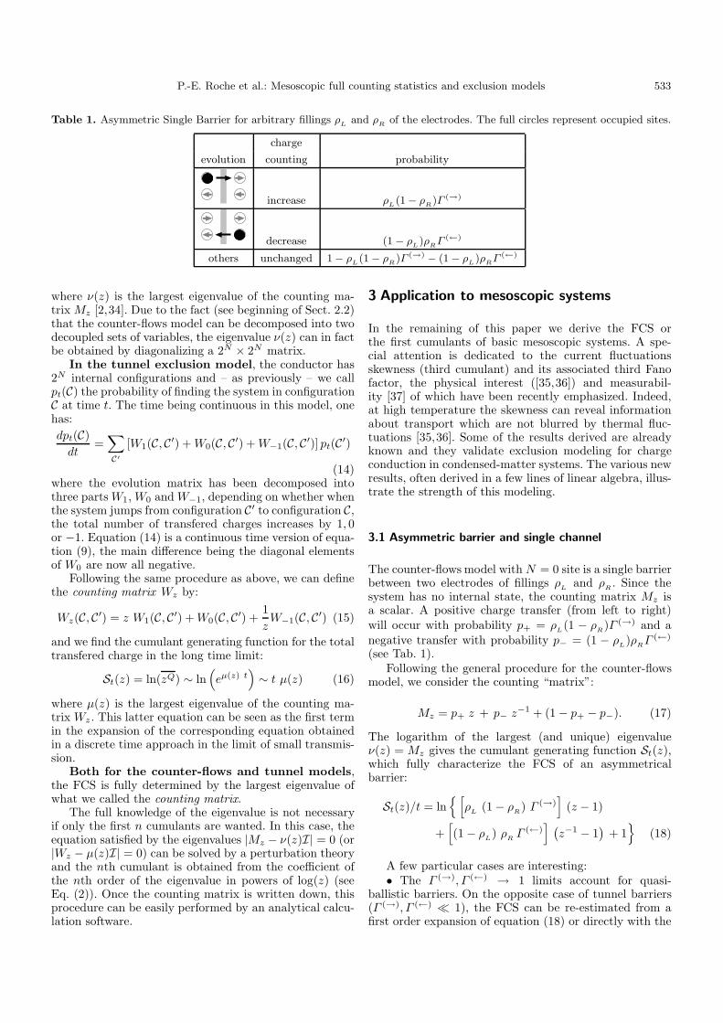
Table 1. Asymmetric Single Barrier for arbitrary fillings ρL and ρR of the electrodes. The full circles represent occupied sites.

charge

evolution counting probability

increase ρL(1 − ρR)Γ (→)

decrease (1 − ρL)ρRΓ (←)

others unchanged 1 − ρL(1 − ρR)Γ (→) − (1 − ρL)ρRΓ (←)

where ν(z) is the largest eigenvalue of the counting ma-trix Mz [2,34]. Due to the fact (see beginning of Sect. 2.2)that the counter-flows model can be decomposed into twodecoupled sets of variables, the eigenvalue ν(z) can in factbe obtained by diagonalizing a 2N × 2N matrix.

In the tunnel exclusion model, the conductor has2N internal configurations and – as previously – we callpt(C) the probability of finding the system in configurationC at time t. The time being continuous in this model, onehas:dpt(C)

dt=

∑C′

[W1(C, C′) + W0(C, C′) + W−1(C, C′)] pt(C′)

(14)where the evolution matrix has been decomposed intothree parts W1, W0 and W−1, depending on whether whenthe system jumps from configuration C′ to configuration C,the total number of transfered charges increases by 1, 0or −1. Equation (14) is a continuous time version of equa-tion (9), the main difference being the diagonal elementsof W0 are now all negative.

Following the same procedure as above, we can definethe counting matrix Wz by:

Wz(C, C′) = z W1(C, C′) + W0(C, C′) +1zW−1(C, C′) (15)

and we find the cumulant generating function for the totaltransfered charge in the long time limit:

St(z) = ln(zQ) ∼ ln(eµ(z) t

)∼ t µ(z) (16)

where µ(z) is the largest eigenvalue of the counting ma-trix Wz . This latter equation can be seen as the first termin the expansion of the corresponding equation obtainedin a discrete time approach in the limit of small transmis-sion.

Both for the counter-flows and tunnel models,the FCS is fully determined by the largest eigenvalue ofwhat we called the counting matrix.

The full knowledge of the eigenvalue is not necessaryif only the first n cumulants are wanted. In this case, theequation satisfied by the eigenvalues |Mz − ν(z)I| = 0 (or|Wz − µ(z)I| = 0) can be solved by a perturbation theoryand the nth cumulant is obtained from the coefficient ofthe nth order of the eigenvalue in powers of log(z) (seeEq. (2)). Once the counting matrix is written down, thisprocedure can be easily performed by an analytical calcu-lation software.

3 Application to mesoscopic systems

In the remaining of this paper we derive the FCS orthe first cumulants of basic mesoscopic systems. A spe-cial attention is dedicated to the current fluctuationsskewness (third cumulant) and its associated third Fanofactor, the physical interest ([35,36]) and measurabil-ity [37] of which have been recently emphasized. Indeed,at high temperature the skewness can reveal informationabout transport which are not blurred by thermal fluc-tuations [35,36]. Some of the results derived are alreadyknown and they validate exclusion modeling for chargeconduction in condensed-matter systems. The various newresults, often derived in a few lines of linear algebra, illus-trate the strength of this modeling.

3.1 Asymmetric barrier and single channel

The counter-flows model with N = 0 site is a single barrierbetween two electrodes of fillings ρ

Land ρ

R. Since the

system has no internal state, the counting matrix Mz isa scalar. A positive charge transfer (from left to right)will occur with probability p+ = ρ

L(1 − ρ

R)Γ (→) and a

negative transfer with probability p− = (1 − ρL)ρRΓ (←)

(see Tab. 1).Following the general procedure for the counter-flows

model, we consider the counting “matrix”:

Mz = p+ z + p− z−1 + (1 − p+ − p−). (17)

The logarithm of the largest (and unique) eigenvalueν(z) = Mz gives the cumulant generating function St(z),which fully characterize the FCS of an asymmetricalbarrier:

St(z)/t = ln{ [

ρL

(1 − ρR) Γ (→)

](z − 1)

+[(1 − ρ

L) ρ

RΓ (←)

] (z−1 − 1

)+ 1

}(18)

A few particular cases are interesting:• The Γ (→), Γ (←) → 1 limits account for quasi-

ballistic barriers. On the opposite case of tunnel barriers(Γ (→), Γ (←) � 1), the FCS can be re-estimated from afirst order expansion of equation (18) or directly with the


tunnel exclusion model with N = 0:

St(z)/t = µ(z) = Wz = ρL(1 − ρ

R)Γ (→)(z − 1)

+ (1 − ρL)ρRΓ (←)(z−1 − 1) (19)

• The asymmetric case (Γ (→) �= Γ (←)) accounts forinelastic barrier, such as those for which stepping over thebarrier requires the emission or assistance of a photon orphonon [35].

For symmetric barriers

T = Γ (→) = Γ (←) (20)

we recover the important case of a conduction channel oftransparency T encountered in mesoscopic transport [12].Once the behavior of a single conduction channel has beendetermined, scattering matrix theory shows how to re-duce the problem of interaction-less electronic transportthrough a quantum constriction into a set of indepen-dent symmetric barriers. In the zero temperature limit,the only states which contribute to the FCS are thosewhose energy ε is such that ρ

L(ε) = 1 and ρ

R(ε) = 0,

or ρL(ε) = 0 and ρ

R(ε) = 1. The FCS is then given as

a superposition of independent binomial laws (“partitionnoise”), one for each of these scattering states, lying inan energy window eV , where V is the voltage drop acrossthe barrier [12]. In the high temperature limit, one hasto integrate the single channel result equation (18) overthe complete Fermi-Dirac distributions in the reservoirs,given in equation (4).

From equations (2), (3), (18) and (T = Γ (→) = Γ (←)),one can derive the normalized noise power F = K2/K1 inthe low temperature limit (Fano factor) and the third Fanofactor F3 = K3/K1 in the high temperature limit [17,35].It is interesting to note that these two quantities turn outto be equal. More generally, for a mesoscopic conductor de-composed into independent channels of transparencies Ti

one has:

F (eV � kBT ) = F3(eV � kBT ) =∑

Ti(1 − Ti)∑Ti

. (21)

The physical information contained in the third cumulantat high temperature [35,36] is the same at the one con-tained in the low temperature second cumulant.

The first equality in equation (21) will be directlychecked for the semi-classical mesoscopic systems consid-ered in the rest of this paper.

3.2 Double barriers

For single barriers, the agreement between the exclusionmodel and mesoscopic models is not surprising since theboundary conditions (injection from the electrodes,...) areidentical. The next step is to assess the validity of exclu-sion models for double barriers, for which it is crucial toaccount properly for both the boundary conditions andthe Pauli exclusion principle inside the conductor.

Fig. 5. Upper figure: Double symmetrical barriers (counter-

flows model with N = 1, = Γ(→)i = Γi). For legibility, the

reflection probabilities 1−Γ1 and 1−Γ2 are not written. Lowerfigure: The internal states of the system.

Double barriers have been widely studied because arich behavior results from the interplay of various effectsincluding Pauli exclusion principle, Coulomb interactions,inelastic processes and quantum resonance [1]. In this sec-tion, we do our calculation on a generic double barrier.Then we see how this system relates to various experimen-tal devices (quantum dots, hopping on localized states,islands and wells) and how the Coulomb interaction be-tween electrons can be introduced to account for chargingeffects. The case of a partly or fully diffusive island be-tween two tunnel barriers is addressed in Section 3.3.

Generic double barrierWe first consider two symmetric barriers of transmis-

sion Γ1 and Γ2, temporarily in the zero temperature limiteV � kBT (ρ

L= 1 and ρ

R= 0). The upper graph of

Figure 5 depicts the corresponding counter-flows model,with N = 1, while the lower graph labels the 22N internalstates of the system.

If the charge counting is done over the second barrier(arbitrary choice), the counting matrix Mz is:

Mz =

Γ1Γ2z Γ1 Γ2z 1(1 − Γ1)Γ2z 1 − Γ1 0 0Γ1(1 − Γ2) 0 1 − Γ2 0

(1 − Γ1)(1 − Γ2) 0 0 0

. (22)

In this matrix, the states are ordered from state-A (upper-left) to state-D (lower-right). The eigenvaluesof Mz can be easily found and the cumulant generat-ing function St(z) is proportional to the logarithm of thelargest one:

St(z)/t = ln

(1 − Γ1 + Γ2 − Γ1Γ2z

2

+

√(1 − Γ1 + Γ2 − Γ1Γ2z

2

)2

− (1 − Γ1) (1 − Γ2)

).

(23)

The symmetry of this expression between Γ1 and Γ2 il-lustrates that the charge counting can be performed on


C2/t =Γ1Γ2Γ

212(ρL + ρR) − (ρ2

L+ ρ2

R)Γ 2

1 Γ 22 (2 − Γ12) − 2ρLρRΓ1Γ2(Γ

21 + Γ 2

2 − Γ1Γ2(Γ1 + Γ2))

Γ 312

. (26)

F3(eV � kBT ) =Γ 4

1 + Γ 42 + Γ 3

1 Γ 32 (4 + Γ1 + Γ2) + Γ 2

1 Γ 22 (6 − 3Γ1 − Γ 2

1 − 3Γ2 − Γ 22 ) − Γ1Γ2(2Γ 2

1 + Γ 31 + 2Γ 2

2 + Γ 32 )

Γ 412

(27)

any side of the system without changing the result. As ex-pected, the single barrier FCS is recovered if one barrieris transparent (Γ1 or Γ2 = 1). Equation (23) extends twoother results first obtained by de Jong in the Boltzmann-Langevin formalism: the first and second cumulants of adouble barrier [27] and the FCS of a double tunnel barrier(Γ1Γ2 � 1) [24]. It is interesting to relate the classical ex-pression equation (23) with the one derived by a full quan-tum treatment of the double barrier system. As describedbelow, such a precise connection may be established in thetunneling regime where both transmissions Γ1 and Γ2 arevery small. A generalization for arbitrary transmissions ispresented in the appendix.

For arbitrary fillings ρL

and ρR

of the electrodes,the counting matrix Mz has no zero element and theeigenvalue problem is still manageable but more tedious.Considering instead the 2 × 2 counting matrix associ-ated with one of the two independent submodels (seebeginning of Sect. 2.2) makes the eigenvalue problemstraightforward again. The power expansion method pre-sented in Section 2.3 is chosen here to derive the cumu-lants C1, C2 and C3, and integration over Fermi-Diracdistribution in the electrodes, according to equations (3)and (4), gives the cumulants K1(eV/kBT ), K2(eV/kBT )and K3(eV/kBT ). It is useful to define:

Γ12 = Γ1 + Γ2 − Γ1Γ2. (24)

One finds

C1/t = (ρL− ρ

R)Γ1Γ2

Γ12(25)

see equation (26 ) above

For eV � kBT , we find K2/K1 = 2kBT/eV , that isthe well known Johnson-Nyquist thermal noise formula,more often written SI = 4kBTG where the conductance Gand the current noise power spectral density SI are givenby equation (5).

We focus now on the third Fano factor F3 = K3/K1.We give below its eV � kBT and eV � kBT limits,which -as would be expected from a quantum mechanicalderivation (Eq. (21)) – is equal to the normalized noisepower F = K2/K1 in the zero temperature limit (Fanofactor). Figure 6 shows that depending of Γ1 and Γ2,the third Fano factor changes sign in the low tempera-ture limit (left Fig. 6) and not in the high temperatureone (right Fig. 6). The insert on the left figure showsF3 = (1 − Γ1Γ2/Γ12)(1 − 2Γ1Γ2/Γ12) obtained when the

exclusion principle is deactivated between the two barri-ers. The change of sign is still observed and thus, it can-not be attributed to correlation inducted by the exclusionprinciple inside the conductor.


F3(eV � kBT ) = 1 − Γ1Γ2(2 − Γ12)Γ 2

12

= F (eV � kBT ).

(28)Tunnel limitThe FCS of a double tunnel barrier can be obtained

from the general expression equation (23) for the doublebarrier. Nevertheless, it is interesting to derive it with theSymmetric Simple Exclusion Model with N = 1. For ar-bitrary fillings ρL and ρR of the electrodes, and chargecounting done over the second barrier, the counting ma-trix is:

Wz =(−Γ2 (1 − ρ

R) − Γ1 (1 − ρ

L) Γ1 ρ

L+ Γ2 ρ

Rz−1

Γ2 (1 − ρR) z + Γ1 (1 − ρ

L) −Γ1 ρ

L− Γ2 ρ

R

).

(29)Following Section 2.3, the cumulant generating func-tion St(z) is proportional to the largest eigenvalue of Wz .After a few lines of algebra, we find:

St(z)/t = −Γ1 + Γ2

2

+

((Γ1 + Γ2

2

)2

+ Γ1Γ2

(ρ

L(1 − ρ

R) (z − 1)

+ ρR

(1 − ρL)(z−1 − 1

)))1/2

. (30)

We recover the FCS derived in [38], which slightly dif-fers from the one derived in [39].

Experimental systemsDepending on the elastic or inelastic nature of the bar-

riers, several double barrier systems are traditionally con-sidered. If we restrict ourselves to elastic barriers, the sizeof the island between the barriers is another source of ex-perimental diversity.

In large but finite-size islands (“quantum island”), thequasi energy levels are discrete and the generic system de-scribed above can model each such level. At this stage, itmay be useful to describe in more detail the connectionbetween a microscopic quantum coherent model for a sin-gle conducting channel in the presence of a double barrier


Fig. 6. Third Fano factor F3 = K3/K1 for a double symmetrical barrier. Left figure: Zero temperature limit (eV � kBT )(insert: the exclusion principle is deactivated between the barriers). Right figure: High temperature limit (kBT � eV ).

in the tunneling limit, and the corresponding SSEP. Atzero temperature, the generating function St(z)/t for themicroscopic quantum model is given by [12]:

St(z)/t = vF

∫ kmax

kmin

dk

2πln(T (k)(z − 1) + 1),

where T (k) is the transmission coefficient for an in-coming electronic wave-function with wave-vector k andkmax − kmin = eV

�vF, vF being the Fermi velocity in the

electrodes. For a fully coherent system, T (k) has to obeythe quantum series composition rule for transmission ma-trices. In the limit of small transmissions T1 and T2, thisyields the well-known Lorentzian resonance profile:

T (k) =4T1T2

(T1 + T2)2 + 16(k − k0)2l2,

where l is the distance between the two barriers. In thelimit where eV/� is much larger than the decay rateγ = vF

2l (T1 +T2) of the resonant level in the central region,and if the average energy of this level is such that k0 fallsin the interval [kmin, kmax], we may take the k integrationover the whole real axis, yielding exactly equation (30) inthe special case ρL(ε) = 1 and ρR(ε) = 0, provided weset Γi = vF

2l Ti (i = 1, 2) [24]. So in the tunnel limit, thesimple SSEP may be viewed as the result of integratingthe contributions of quantum-mechanically coherent elec-trons over an energy window larger than the width �γof a discrete level inside the cavity delimited by the twobarriers.

When the island is infinite in the transverse direction(“Quantum well”), the energy levels become a continu-ous energy band: the generic model still applies but theintegration equation (3) should be done versus wavevec-tors [1] k‖ (longitudinal) and k⊥ (transverse direction)rather than versus the energy ε.

Finally, when the island is small (“Quantum dot”) orwhen it consists in localized states (dopants, impurities...),

Fig. 7. Left figure: Energy levels associated with the two sitesin interaction. Right figure: The three internal states of thesystem. Each black disk represents an electron and each circlerepresents an available site with spin degeneracy.

the energy levels are well separated but one can no longerneglect that electrons entering or leaving the island arechanging its Coulomb electrostatic energy, which induces ashift of the energy levels (“charging effect”). We illustratein the simple example below how to account for such aneffect.

Charging effectWe consider now two localized states tunnel-coupled

to two electrodes with Fermi-Dirac fillings ρL(ε) and ρ

R(ε)

(Fig. 7). The coupling is elastic (for example, it could bedue to some overlapping of the localized state wavefunc-tion with electrodes) and characterized by two symmet-rical transmission coefficients Γ1, Γ2 � 1. So we assumethat an electron can be transfered from one electrode tothe other by a sequential tunneling process through one ofthe two localized states. Because of large on-site Coulombinteraction, at most one electron, with spin up or down,can be trapped on each localized state. To model intersitecharging effects, we assume that the localized sites contri-bution to the energy is Eloc(n1, n2) = ε1n1+ε2n2+Un1n2

where n1 and n2 are the occupation numbers, ε1 and ε2are the single level energies and U > 0 is an electrostaticenergy. Such a model has already been proposed [40] toexplain experimental data. Our purpose in this section is


Wz = Γ

−4ρL(ε0) − 4ρR(ε0) (1 − ρL(ε0)) + (1 − ρR(ε0))z 04ρL(ε0) + 4ρR(ε0)/z − 2 + ρL(ε0) − 2ρL(ε+) + ρR(ε0) − 2ρR (ε+) 2(1 − ρL(ε+)) + 2(1 − ρR(ε+))z

0 2ρL(ε+) + 2ρR(ε+)/z − 4 + 2ρL(ε+) + 2ρR(ε+))

(31)

Fig. 8. Two sites interacting via the Coulomb electrostaticrepulsion and tunnel coupled to electrodes (see text). Left fig-ure: Normalized current C1/(t4Γ/3). Central figure: Normal-ized noise power C2/C1. Right figure: Third Fano factor C3/C1.

to illustrate how exclusion models can deal with charg-ing effect. For the sake of clarity, we therefore restrictedourselves to degenerated energy levels ε0 = ε1 = ε2 andΓ = Γ1 = Γ2. This system has three internal states, corre-sponding to 0, 1 or 2 trapped electrons (States A, B and Cin Fig. 7) and the corresponding counting matrix is


where ε+ = ε0 +U . With a software like Mathematica, theanalytical equations for the cumulants C1, C2 and C3 areeasily derived by the series expansion method (Sect. 2.3).These expressions are not reported here but have beenused to generate the normalized cumulants of Figure 8 forparameters ε0/kBT = 10, U/kBT = 20 and Γ � 1. Thefirst cumulant C1 is normalized by the averaged transfercharge 4.t.Γ/3 expected in the high driving voltage limit.

Similar stochastic classical models have also been stud-ied to account for transport through quantum dot abovethe Kondo temperature (see for example [38,41,42]). Be-low this temperature, classical models are no longer ex-pected to be meaningful.

3.3 Multiple barriers: from double wells to diffusiveislands between tunnel contacts

In this section we discuss the general SSEP model pre-sented at the end of Section 2.2 , (N −1) identical barriersof transmission Γ � 1 are sandwiched between two tun-nel barriers of transmission Γ

Land Γ

R. Although a single

chain of sites is considered, this situation is expected toaccount for physical systems with a large number of trans-verse conduction channels. This is justified a-posteriori bythe perfect quantitative agreement between the predic-tions of the classical models and the full quantum mechan-ical derivation for multi-channels systems (see below).

Writing down that the mean current and its vari-ance do not depend on the barrier over which they

are measured, we showed in [2] how to derive the firsttwo cumulants:

C1/t =Γ

N1(ρ

L− ρ

R) (32)

C2/t =Γ

N1

[(ρ

L+ ρ

R− 2ρ

Lρ

R)

− 23(ρ

L− ρ

R)2

(1 − 1

2N1− λ

2N12 (N1 − 1)

)](33)

with N1 = N − 1 + ΓΓ

L+ Γ

ΓR

and λ =ΓΓ

L

(Γ

ΓL− 1

)(2 Γ

ΓL− 1

)+ Γ

ΓR

(Γ

ΓR− 1

)(2 Γ

ΓR− 1

)

For arbitrary N1, the third cumulant C3 can be derivedfrom the third order series expansion of the cumulant gen-erating function given in [2] (Eq. (C.14)). We give belowthe third Fano factor in the large N1 (or N) limit.

Experimental systemsThree limiting cases of the above general formula could

be relevant to mesophysics.• Firstly, for N = 2, the system is a triple barrier

with three different tunnel transmissions. Such systemshave been widely studied as a model for double localizedstate, coupled quantum dot and double well structures (forexample see [1,43]). It would be interesting to compare ourpredictions to the experimental results.

• In the limit N → ∞ for constant Γ , ΓL

and ΓR,

the relative contribution of the two out-most barriers isvanishingly small and we obtain a diffusive medium ingood contact with the electrodes. Section 3.4 addressesthis purely diffusive regime and gives its FCS. At thispoint, we just point that C1 and C2 are in agreementwith the one found by alternative condensed-matter for-malisms [22,27,44–48]. It is specially interesting to notethat a one dimensional classical stochastic model is able toreproduce current fluctuations arising in a 3 dimensionalcoherent diffusive conductor.

• The limit N → ∞ for constant Γ , NΓL

and NΓR

ac-counts for a diffusive island between two tunnel contacts,the resistances of which are comparable to the resistanceof the diffusive island itself. We define as qL = Γ/(NΓL)and q

R= Γ/(NΓ

R) the ratios of the left and right con-

tact resistances over the diffusive island resistance. Thelarge q

Land q

Rlimit accounts for simple or double tunnel

barriers while vanishing values of qL

and qR

account for apurely diffusive medium.

The normalized noise power F (Eq. (6)), is found tobe, for an arbitrary temperature:

F =K2

K1=

2kBT

eV(1 − s) + s coth

(eV

2kBT

)(34)


Table 2. First cumulants Cn for diffusive medium for arbitrary filling of the electrodes, and low and high temperature normalizedcumulants Kn/K1. (X = (ρL − ρR) and Y = (ρL + ρR − 1)).

Kn/K1 Kn/K1

n Normalized cumulants: Cn(tΓ/N)

for for

kBT � eV kBT � eV

1 X 1 1

2[3 − X2 − 3Y 2] /6 1

32kBT

eV

3 X3/15 + XY 2 115

13

4[−9X4 + X2 (

7 − 462Y 2) − 105Y 2 (−1 + Y 2)] /210 − 1105

2kBT3eV

5 4X5/105 + XY 2(−3 + 4Y 2

)+ X3

(−1 + 120Y 2)/21 − 1

105− 1

5

6 [−20X6 − 33X4(−1 + 244Y 2

) − 231Y 2(3 − 7Y 2 + 4Y 4

)−11X2

(1 − 618Y 2 + 1044Y 4

)]/462 1

231− 2kBT

5eV

with

s =13

+2(q3

L+ q3

R

)

3 (1 + qL

+ qR)3

. (35)

The well known noise power of double tunnel barri-ers [1,49,50] and diffusive media [22,27,44–48] are recov-ered in the large and small qL , qR limits. The third Fanofactor is found to be:

F3 =K3

K1= 1 +

kBT

eV3 (s − 1 − 2f) coth

(eV

2kBT

)

+f − 3(s − 1)/2 + 2f

[cosh( eV

2kBT )]2

[sinh( eV

2kBT )]2 (36)

with

f = − 310

+ 3s (s − 1/2)−6(q5

L+ q5

R)

5(1 + qL

+ qR)5

(37)

Equation (36) bridges continuously between two sim-ple situations: double tunnel barriers (large q

L, q

R) and

diffusive media (small qL, q

R) for which we also recover

known results [17,23]. In the low and high temperaturelimits, we found:

F3(eV � kBT ) = 1 + 2f

F3(eV � kBT ) = s = F (eV � kBT ). (38)

The high temperature skewness is equal to the low tem-perature noise power, as would be expected from a fullyquantum treatment (see Eq. (21)).

3.4 Diffusive medium

In this section, we consider a diffusive medium with goodcontacts to the electrodes.

We first consider the SSEP model in the N → ∞ limit,which is enough to account for a purely diffusive behavior.At the end of this section, we consider the cross-over froma ballistic to diffusive conduction. To do so, the counter-flows model will be required.

SSEP diffusive mediumIn our previous paper [2], we detail the derivation of

the FCS for SSEP models in the N → ∞ limit and we shallonly summarize the results here. The cumulant generatingfunction St depends on N , z, ρL and ρR but to first orderin 1/N , St turns out to depend only on a combination ωof these parameters:

ω =(z − 1)(ρLz − ρR − ρLρR(z − 1))

z. (39)

Consequently, to first order in 1/N one can write:

St/t =Γ

NR(ω) (40)

where the expression of R(ω) has been conjectured. Thus,if the FCS is known for two arbitrary fillings of the elec-trodes, then it can be deduced for any fillings or at anytemperature.

Based on the exact derivation of the first 4 cumulants,we conjectured that for ρL = ρR = 1/2, the statisticsof current fluctuations is Gaussian (at order 1/N). Thisfully determines R(ω) and thus the current statistics at aarbitrary fillings ρ

Land ρ

R:

St/t =Γ

N

[log(

√1 + ω +

√ω)

]2. (41)

This expression is identical to the one found at zerotemperature by [15] and at arbitrary temperature by [17](and by [51] with minor discrepancies). Table 2 givesthe first cumulants Cn, Kn/K1 for kBT � eV and forkBT � eV . Right/Left symmetry and particle/hole sym-metry suggest the change of parameters: X = (ρ

L− ρ

R)

and Y = (ρL

+ ρR− 1). Agreement is found with the first

four cumulants which can be easily derived from [23] (af-ter correcting a typo: the last x in equation (24) shouldbe an x1).

Ballistic-diffusive cross-overWe now consider a counter-flows model with uniform

symmetrical transmission coefficients Γ in the bulk of theconductor (Γ = Γ

(→)i = Γ

(←)i for 1 < i < N + 1), unity


Fig. 9. Third Fano factor K3/K1 in a ballistic/diffusivemedium parametrized by the ratio L/Lelast of the conductor’slength L over a elastic mean free path Lelast (counter-flowswith N = 8). The two lines correspond to known limit forL/Lelast � 1 (continuous line) and for L/Lelast � 1 witheV � kBT (pearly line).

transmission at the boundaries (Γ (←)1 = Γ

(→)1 = Γ

(←)N+1 =

Γ(→)N+1 = 1), and we consider the N → ∞ limit taken at

constant (1−Γ )(N−1). We can define the mean free pathLelast of a single electron as 1/(1 − Γ ) and the lengthL of the conductor as N − 1. Then (1 − Γ )(N − 1) =L/Lelast � 1 corresponds to a ballistic conductor whileL/Lelast � 1 to a diffusive one [28,52]. We explore thethird Fano factor F3 = K3/K1 versus both the ballistic-diffusive cross-over and the thermal (kBT � eV ) - shotnoise (eV � kBT ) cross-over. At zero temperature, it wasshown [26] that N as small as 8 gives a correct picture ofthe skewness, even in the diffusive limit. We performed anumerical simulation of such a small N by solving numer-ically the largest eigenvalue of the counting matrix. Fig-ure 9 shows F3(L/Lelast, eV/kBT ). For comparison, thecontinuous line is calculated from the analytical results inthe diffusive limit and good agreement is found with thenumerical estimation. This is an interesting result, whichshows a tendency of the simple exclusion model to repro-duce the same FCS as for a larger class of models. Thisraises the question of trying to identify more precisely thekey features which are required for a stochastic model toyield this FCS. The pearly line corresponds to a singlescatterer with the same conductance as the system in thelow temperature limit. As L/Lelast → 0 (L may be arbi-trary large), the system is expected to converge to such apoint scatterer limit and a good agreement is found withthe simulation. Good agreement is also found with Monte-Carlo simulations performed along the ballistic-diffusivecross-over at zero temperature [26].

4 Concluding remarks

In this paper, we have checked explicitly that the FCSof purely classical stochastic models with a local exclu-sion constraint coincides with the FCS of a large class of

quantum mechanical microscopic models where the cur-rent flows between two reservoirs. In particular, no restric-tion on the system size seems to be necessary, since thiscoincidence appears for a small number of tunnel barriers,as well as in the limit of a diffusive medium composed of anarbitrary large number of such barriers. The two key com-mon ingredients to both types of models are the stochasticnature of scattering processes and the constraint removingdoubly occupied sites, imposed by the Pauli principle. Thefirst ingredient establishes a very interesting difference be-tween classical Hamiltonian mechanics, where diffusion isa chaotic but deterministic process, and quantum mechan-ics, where an intrinsic notion of probability arises. Thisdistinction is the same as the difference between ray andwave optics. As shown in [53], the crossover from the firstregime to the second occurs when the typical time spentby a wave-packet in the system becomes larger than theEhrenfest time associated to the spreading of this wave-packet induced by the underlying chaotic dynamics. Ourstochastic models require physical systems dominated bydiffractive scattering.

This work raises the question of the role of space di-mensionality in the FCS of classical exclusion models. Itwould also be very interesting to extend the classical ap-proach in terms of exclusion models to multi-terminal ge-ometries. Such generalizations have been considered ina fully quantum-mechanical treatment of diffusive sys-tems [47], or in the semi-classical Boltzmann-Langevin ap-proach [48]. These works have so far focused on the cor-relation matrix of the integrated charges flowing througheach contact during a finite time interval. A natural ques-tion is whether simple classical exclusion models are ableto generate these results for the second order cumulants.The computation of higher-order cumulants in multi-terminal geometries is another interesting open question.

5 Appendix: Quantum treatment of a doublebarrier

We consider here the quantum version of the calculationfor a double barrier of Section 3.2, but adapted to the casewhere transmissions T1, T2 are not assumed to be small.Our starting point is the composition rule for the series oftwo barriers:

t =t1t2

1 − r′1r2=

t1t21 − |r1||r2|eiφ

(42)

where Ti = |ti|2, and |ti|2 + |ri|2 = 1. We have seen thatwhen both T1 and T2 are small, integrating over thephase φ of r′1r2 with a uniform weight yields the FCS of thecounter-flows model, in the limit where Γ1, Γ2 � 1, whichcoincides with the FCS of the Symmetric Simple Exclu-sion Model for a double barrier. This integration over thephase-shift φ is motivated in this case by the fact that |t|2exhibits a sharp resonance as a function of φ. So even fora single coherent channel, a rather small voltage drop in-duces an energy spread for the incoming electrons which


is larger than the energy width of the resonance, therebyjustifying the φ integration.

When Ti’s are no longer small, |t(φ)| becomes a rathersmooth function of φ, and resonances tend to disappear,since the inner regions between the barriers is now wellcoupled to reservoirs. For a single channel, averagingover φ takes place only if:

eV � �2kF

ml. (43)

For smaller voltages, the FCS becomes a binomial lawobtained by the quantum series composition rule equa-tion (42), where the phase-shift is taken at the Fermi level.In this case, it is clear that the FCS of the counter-flowsmodel given by equation (23) does not agree with the fullquantum treatment, since the former has lost all informa-tion on phases of reflection coefficients.

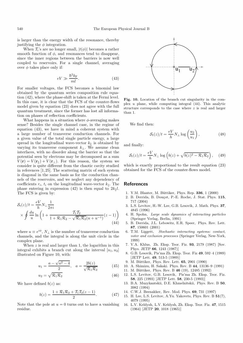
What happens in a situation where φ-averaging makessense? Besides the single channel case, in the regime ofequation (43), we have in mind a coherent system witha large number of transverse conduction channels. Fora given value of the total single particle energy, a largespread in the longitudinal wave-vector k‖ is obtained byvarying its transverse component k⊥. We assume cleaninterfaces, with no disorder along the barrier so that thepotential seen by electrons may be decomposed as a sumV (r) = V (r‖) + V (r⊥). For this reason, the system weconsider is quite different from the chaotic cavity studiedin references [1,25]. The scattering matrix of such systemis diagonal in the same basis as for the conduction chan-nels of the reservoirs, and we neglect any dependency ofcoefficients ri, ti on the longitudinal wave-vector k‖. Thephase entering in expression (42) is then equal to 2k‖l.The FCS is given by:

St(z)/t =eV

hN⊥

12πi

×∮

du

uln

(1 +

T1T2

1 + R1R2 −√R1R2(u + u−1)

(z − 1))

(44)

where u ≡ eiφ, N⊥ is the number of transverse conductionchannels, and the integral is along the unit circle in thecomplex plane.

When z is real and larger than 1, the logarithm in thisintegral exhibits a branch cut along the interval [u1, u2]illustrated on Figure 10, with:

u1 =a −

√a2 − 42

, a =2b(z)√R1R2

(45)

u2 =√R1R2 (46)

We have defined b(z) as:

b(z) =1 + R1R2 + T1T2(z − 1)

2. (47)

Note that the pole at u = 0 turns out to have a vanishingresidue.

Fig. 10. Location of the branch cut singularity in the com-plex u plane, while computing integral (44). This analyticstructure corresponds to the case where z is real and largerthan 1.

We find then:

St(z)/t =eV

hN⊥ log

(u2

u1

), (48)

and finally:

St(z)/t =eV

hN⊥ log

(b(z) +

√b(z)2 −R1R2

), (49)

which is exactly proportional to the result equation (23)obtained for the FCS of the counter-flows model.

References

1. Y.M. Blanter, M. Buttiker, Phys. Rep. 336, 1 (2000)2. B. Derrida, B. Doucot, P.-E. Roche, J. Stat. Phys. 115,

717 (2004)3. L.S. Levitov, H.-W. Lee, G.B. Lesovik, J. Math. Phys. 37,

4845 (1996)4. H. Spohn, Large scale dynamics of interacting particles

(Springer Verlag, Berlin, 1991)5. B. Derrida, J.L. Lebowitz, E.R. Speer, Phys. Rev. Lett.

87, 150601 (2001)6. T.M. Liggett, Stochastic interacting systems: contact,

voter and exclusion processes (Springer Verlag, New-York,1999)

7. V.A. Khlus, Zh. Eksp. Teor. Fiz. 93, 2179 (1987) [Sov.Phys. JETP 66, 1243 (1987)]

8. G.B. Lesovik, Pis’ma Zh. Eksp. Teor. Fiz 49, 592–4 (1989)[JETP Lett. 49, 513-5 (1989)]

9. M. Buttiker, Phys. Rev. Lett. 65, 2901 (1990)10. A. Shimizu, H. Sakaki. Phys. Rev. B 44, 13136–9 (1991)11. M. Buttiker, Phys. Rev. B 46 (19), 12485 (1992)12. L.S. Levitov, G.B. Lesovik, Pis’ma Zh. Eksp. Teor. Fiz.

58, 225 (1993) [JETP Lett. 58, 230-5 (1993)]13. B.A. Muzykantskii, D.E. Khmelnitskii, Phys. Rev. B 50,

3982 (1994)14. C.W.J. Beenakker, Rev. Mod. Phys. 69, 731 (1997)15. H. Lee, L.S. Levitov, A.Yu. Yakovets, Phys. Rev. B 51(7),

4079 (1995)16. L.V. Keldysh, L.V. Keldysh, Zh. Eksp. Teor. Fiz. 47, 1515

(1964) [JETP 20, 1018 (1965)]


17. D.B. Gutman, Y. Gefen, A.D. Mirlin, in QuantumNoise in Mesoscopic Physics, edited by Y.V. Nazarov,pages 497−524 (Kluwer Academic Publishers, Dordreicht,2003), pp. 497–524

18. Y.V. Nazarov, in Quantum dynamics of submicron struc-tures, edited by H. Cerdeira, B. Kramer, G. Schoen, 1995,p. 687

19. Y.V. Nazarov, D.A. Bagrets, Phys. Rev. Lett. 88, 196801(2002)

20. A.Ya. Shulman, Sh.M. Kogan, Zh. Eksp. Teor. Fiz. 57,2112 (1969) [Sov. Phys. JETP 29, 3 (1969)]

21. S.V. Gantsevich, V.L. Gurevich, R. Katilius, Sov. Phys.JETP 30, 276 (1970)

22. K.E. Nagaev, Phys. Lett. A 169, 103 (1992)23. K.E. Nagaev, Phys. Rev. B 66, 075334 (2002)24. M.J.M. de Jong, Phys. Rev. B 54, 8144 (1996)25. S. Pilgram, A.N. Jordan, E.V. Sukhorukov, M. Buttiker,

Phys. Rev. Lett. 90, 206801 (2003)26. P.-E. Roche, B. Doucot, Eur. Phys. J. B 27, 393 (2002)27. M.J.M. de Jong, C.W.J. Beenakker, Phys. Rev. B 51,

16867 (1995)28. R.C. Liu, P. Eastman, Y. Yamamoto, Solid. State Comm.

102, 785 (1997)29. B. Yurke, G.P. Kochanski, Phys. Rev. B 41, 8184 (1990)30. R. Landauer, T. Martin, Physica B 175, 167 (1991)31. M. Reznikov, M. Heiblum, H. Shtrikman, D. Mahalu,

Phys. Rev. Lett. 75, 3340 (1995)32. A. Kumar, L. Saminadayar, D.C. Glattli, Phys. Rev. Lett.

76, 2778 (1996)33. H. Spohn, J. Phys. A 16, 4275 (1983)34. B. Derrida, J.L. Lebowitz, Phys. Rev. Lett. 80, 209 (1998)35. L.S. Levitov, M. Reznikov, cond-mat/0111057, 2001 (see

also Phys. Rev. B 70, 115305 (2004))36. D.B. Gutman, Y. Gefen, Phys. Rev. B 68, 035302 (2003)37. B. Reulet, J. Senzier, D.E. Prober, Phys. Rev. Lett. 91,

196601 (2003)

38. D.A. Bagrets, Y.V. Nazarov, Phys. Rev. B 67, 085316(2003)

39. W. Belzig, in Quantum Noise in Mesoscopic Physics,edited by Y.V. Nazarov (Kluwer Academic Publishers,Netherlands, 2003), pp. 469–496

40. A.K. Savchenko, S.S. Safonov, S.H. Roshko, D.A. Bagrets,O.N. Jouravlev, Y.V. Nazarov, E.H. Linfield, D.A. Ritchie,Physica Status Solidi (b) 241, 26 (2004)

41. L.I. Glazman, K.A. Matveev, Pis’ma Zh. Eksp. Teor. Fiz.48, 403 (1988) [JETP Lett. 48, 445 (1988)]

42. S. Hershfield, J.H. Davies, P. Hyldgaard, C.J. Stanton,J.W. Wilkins, Phys. Rev. B 47, 1967 (1993)

43. Y.A. Kinkhabwala, A.N Korotkov, Phys. Rev. B 62, R7727(2000)

44. C.W.J. Beenakker, M. Buttiker, Phys. Rev. B 46, 1889(1992)

45. Y.V. Nazarov, Phys. Rev. Lett. 73(1), 134 (1994)46. B.L. Al’tshuler, L.S. Levitov, A.Yu. Yakovets, Pis’ma

Zh. Eksp. Teor. Fiz. 59, 821 (1994) [JETP Lett. 59, 857(1994)]

47. Y.M. Blanter, M. Buttiker, Phys. Rev. B 56, 2127 (1997)48. E.V. Sukhorukov, D. Loss, Phys. Rev. Lett. 80, 4959

(1998)49. L.Y. Chen, C.S. Ting, Phys. Rev. B 43, 4534 (1991)50. J.H. Davies, P. Hyldgaard, S. Hershfield, J.W. Wilkins,

Phys. Rev. B 46, 9620 (1992)51. Y.V. Nazarov, Ann. Phys (Leipzig) 8, Spec. Issue SI-193,

507 (1999)52. M.J.M. de Jong, C.W.J. Beenakker, in Mesoscopic electron

transport, edited by L.P. Kouwenhoven, G. Schon, L.L.Sohn, Vol. 345 of NATO Advances Studies Institute (ASI)Series E: Applied Sciences (Kluwer Academic Plublishers,Dordrecht, 1996)

53. O. Agam, I. Aleiner, A. Larkin, Phys. Rev. Lett. 85, 3153(2000)

Documents

Mesoscopic full counting statistics and exclusion models