Embed Size (px)
Citation preview
Psychological Methods2001, Vol. 6, No. 2, 161-180
Copyright 2001 by the American Psychological Association, Inc.1082-989X/01/S5.00 DOI: 10.1037//1082-989X.6.2.161
Meta-Analysis of Correlation Coefficients: A Monte CarloComparison of Fixed- and Random-Effects Methods
Andy P. FieldUniversity of Sussex
The efficacy of the Hedges and colleagues, Rosenthal-Rubin, and Hunter-Schmidtmethods for combining correlation coefficients was tested for cases in which popu-lation effect sizes were both fixed and variable. After a brief tutorial on thesemeta-analytic methods, the author presents two Monte Carlo simulations that com-pare these methods for cases in which the number of studies in the meta-analysisand the average sample size of studies were varied. In the fixed case the methodsproduced comparable estimates of the average effect size; however, the Hunter-Schmidt method failed to control the Type I error rate for the associated signifi-cance tests. In the variable case, for both the Hedges and colleagues and Hunter-Schmidt methods, Type I error rates were not controlled for meta-analysesincluding 15 or fewer studies and the probability of detecting small effects was lessthan .3. Some practical recommendations are made about the use of meta-analysis.
Meta-analysis is a statistical technique by whichinformation from independent studies is assimilated.Traditionally, social science literatures were assimi-lated through discursive reviews. However, such re-views are subjective and prone to "reviewer biases"such as the selective inclusion of studies, selectiveweighting of certain studies, and misrepresentation offindings (see Wolf, 1986). The inability of the humanmind to provide accurate, unbiased, reliable, and validsummaries of research (Glass, McGaw, & Smith,1981) created the need to develop more objectivemethods. Meta-analysis arguably provides the firststep to such objectivity (see Schmidt, 1992), althoughit too relies on subjective judgments regarding studyinclusion (and so is still problematic because of biasedselections of studies, and the omission of unpublisheddata—the file drawer problem; see Rosenthal & Ru-bin, 1988). Since the seminal contributions of Glass(1976), Hedges and Olkin (1985), Rosenthal and Ru-bin (1978), and Hunter, Schmidt, and Jackson (1982)there has been a meteoric increase in the use of meta-analysis. A quick search of a social science database1
revealed over 2,200 published articles using or dis-
Correspondence concerning this article should be ad-dressed to Andy P. Field, Psychology Group, School ofCognitive and Computing Science, University of Sussex,Palmer, Brighton, East Sussex BN1 9QH, United Kingdom.Electronic mail may be sent to [email protected].
cussing meta-analysis published between 1981 and2000. Of these, over 1,400 have been published since1995, and over 400 in the past year. Clearly, the useof meta-analysis is still accelerating, and conse-quently the question of which technique is best hasarisen.
Methods of Meta-Analysis forCorrelation Coefficients
Basic PrinciplesTo summarize, an effect size refers to the magni-
tude of effect observed in a study, be that the size ofa relationship between variables or the degree of dif-ference between group means. There are many differ-ent metrics that can be used to measure effect size: thePearson product-moment correlation coefficient, r;the effect-size index, d; as well as odds ratios, riskrates, and risk differences. Of these, the correlationcoefficient is used most often (Law, Schmidt, &Hunter, 1994) and so is the focus of the present study.Although various theorists have proposed variationson these metrics (e.g., Glass's A, Cohen's d, andHedges's g are all estimates of 8), conceptually eachmetric represents the same thing: a standardized formof the size of the observed effect. Whether correlationcoefficients or measures of differences are calculatedis irrelevant because either metric can be convertedinto the other, and statistical analysis procedures for
1 The Web of Science was used (http://wos.mimas.ac.uk).
161

162 FIELD
different metrics differ only in how the standard errorsand bias corrections are calculated (Hedges, 1992).
In meta-analysis, the basic principle is to calculateeffect sizes for individual studies, convert them to acommon metric, and then combine them to obtain anaverage effect size. Studies in a meta-analysis aretypically weighted by the accuracy of the effect sizethey provide (i.e., the sampling precision), which isachieved by using the sample size (or a function of it)as a weight. Once the mean effect size has been cal-culated it can be expressed in terms of standard nor-mal deviations (a Z score) by dividing by the standarderror of the mean. A significance value (i.e., the prob-ability, p, of obtaining a Z score of such magnitude bychance) can then be computed. Alternatively, the sig-nificance of the average effect size can be inferredfrom the boundaries of a confidence interval con-structed around the mean effect size.
Johnson, Mullen, and Salas (1995) pointed out thatmeta-analysis is typically used to address three gen-eral issues: central tendency, variability, and predic-tion. Central tendency relates to the need to find theexpected magnitude of effect across many studies(from which the population effect size can be in-ferred). This need is met by using some variation onthe average effect size, the significance of this aver-age, or the confidence interval around the average.The issue of variability pertains to the difference be-tween effect sizes across studies and is generally ad-dressed with tests of the homogeneity of effect sizes.The question of prediction relates to the need to ex-plain the variability in effect sizes across studies interms of moderator variables. This issue is usuallyaddressed by comparing study outcomes as a functionof differences in characteristics that vary over all stud-ies. As an example, differences in effect sizes couldbe moderated by the fact that some studies were car-ried out in the United States whereas others were con-ducted in the UK.
Fixed- Versus Random-Effects Models
So far, we have seen that meta-analysis is used as away of trying to ascertain the true effect size (i.e., theeffect size in a population) by combining effect sizesfrom individual studies. There are two ways to con-ceptualize this process: fixed-effects and random-effects models.2 Hedges (1992) and Hedges andVevea (1998) explained the distinction between thesemodels wonderfully. In essence, in the fixed-effectsconceptualization, the effect sizes in the populationare fixed but unknown constants. As such, the effect
size in the population is assumed to be the same for allstudies included in a meta-analysis (Hunter &Schmidt, in press). This situation is called the homo-geneous case. The alternative possibility is that thepopulation effect sizes vary randomly from study tostudy. In this case each study in a meta-analysiscomes from a population that is likely to have a dif-ferent effect size than any other study in the meta-analysis. Therefore, population effect sizes can bethought of as being sampled from a universe of pos-sible effects—a "superpopulation" (Becker, 1996;Hedges, 1992). This situation is called the heteroge-neous case. To summarize, in the random-effectsmodel studies in the meta-analysis are assumed to beonly a sample of all possible studies that could bedone on a given topic, whereas in the fixed-effectsmodel the studies in the meta-analysis are assumed toconstitute the entire universe of studies (Hunter &Schmidt, in press).
In statistical terms the main difference betweenthese models is in the calculation of standard errorsassociated with the combined effect size. Fixed-effects models use only within-study variability intheir error term because all other "unknowns" in themodel are assumed not to affect the effect size (seeHedges, 1992; Hedges & Vevea, 1998). However, inrandom-effects models it is necessary to account forthe errors associated with sampling from populationsthat themselves have been sampled from a superpopu-lation. As such the error term contains two compo-nents: within-study variability and variability arisingfrom differences between studies (see Hedges &Vevea, 1998). The result is that standard errors in therandom-effects model are typically much larger thanin the fixed case if effect sizes are heterogeneous, andtherefore, significance tests of combined effects aremore conservative.
In reality the random-effects model is probablymore realistic than the fixed-effects model on the ma-jority of occasions (especially when the researcherwishes to make general conclusions about the re-search domain as a whole and not restrict his or herfindings to the studies included in the meta-analysis).Despite this fact, the National Research Council(1992) reports that fixed-effects models are the rule
2 In reality it is possible to combine fixed- and random-effects conceptualizations to produce a mixed model. Forthe purpose of this study the mixed model is ignored, but theinterested reader is referred to Hedges (1992).
META-ANALYSIS OF CORRELATION COEFFICIENTS 163
rather than the exception. Osburn and Callender(1992) have also noted that real-world data are likelyto have heterogeneous population effect sizes even inthe absence of known moderator variables (see alsoSchmidt & Hunter, 1999). Despite these observations,Hunter and Schmidt (in press) reviewed the meta-analytic studies reported in Psychological Bulletin (amajor review journal in psychology) and found 21studies reporting fixed-effects meta-analyses but noneusing random-effects models. Although fixed-effectsmodels have attracted considerable attention (Hedges,1992, 1994a, 1994b), as Hedges and Vevea (1998)pointed out, the choice of model depends largely onthe type of inferences that the researcher wishes tomake: fixed-effects models are appropriate only forconditional inferences (i.e., inferences that extendonly to the studies included in the meta-analysis),whereas random-effects models facilitate uncondi-tional inferences (i.e., inferences that generalize be-yond the studies included in the meta-analysis). Forreal-world data in the social sciences researchers typi-cally wish to make unconditional inferences, so ran-dom-effects models are often more appropriate.
Over the past 20 years, three methods of meta-analysis have remained popular (see Johnson et al.,1995): the methods devised by Hedges, Olkin, andcolleagues; by Rosenthal and Rubin (see Rosenthal,1991); and by Hunter and Schmidt (1990).3 Hedgesand colleagues (Hedges, 1992; Hedges & Olkin,1985; Hedges & Vevea, 1998) have developed bothfixed- and random-effects models for combining ef-fect sizes, whereas Rosenthal (1991) presented only afixed-effects model and Hunter and Schmidt pre-sented what they have labeled a random-effects model(see Schmidt & Hunter, 1999). Although Johnson etal. (1995) provided an overview of these three meta-analytic techniques, they did not use the methods forcorrelation advocated by Hedges and colleagues (oruse the random-effects versions), and Schmidt andHunter (1999) have made subsequent observationsabout the correct use of their method. Therefore, anoverview of the techniques used in the current study,with reference to the original sources, is included as apedagogical source for readers unfamiliar with meta-analysis of correlation coefficients.
The Hedges-Olkin and Rosenthal-RubinMethods
For combining correlation coefficients, Hedges andOlkin (1985), Hedges and Vevea (1998), and Rosen-thai and Rubin (see Rosenthal, 1991) were in agree-
ment about the method used. However, there are twodifferences between the treatments that Hedges andcolleagues and Rosenthal and Rubin have given to themeta-analysis of correlations. First, Rosenthal (1991)did not present a random-effects version of the model.Second, to estimate the overall significance of themean effect size, Rosenthal and Rubin generally ad-vocated that the probabilities of each effect size oc-curring by chance be combined (see Rosenthal, 1991;Rosenthal & Rubin, 1982).
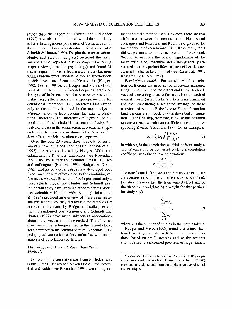
Fixed-effects model. For cases in which correla-tion coefficients are used as the effect-size measure,Hedges and Olkin and Rosenthal and Rubin both ad-vocated converting these effect sizes into a standardnormal metric (using Fisher's r-to-Z transformation)and then calculating a weighted average of thesetransformed scores. Fisher's r-to-Z transformation(and the conversion back to r) is described in Equa-tion 1 . The first step, therefore, is to use this equationto convert each correlation coefficient into its corre-sponding Z value (see Field, 1999, for an example):
in which r, is the correlation coefficient from study i.This Z value can be converted back to a correlationcoefficient with the following equation:
r ,= -
The transformed effect sizes are then used to calculatean average in which each effect size is weighted.Equation 2 shows that the transformed effect size ofthe jth study is weighted by a weight for that particu-lar study (vv;):
k
(2)
where k is the number of studies in the meta-analysis.Hedges and Vevea (1998) noted that effect sizes
based on large samples will be more precise thanthose based on small samples and so the weightsshould reflect the increased precision of large studies.
3 Although Hunter, Schmidt, and Jackson (1982) origi-nally developed this method, Hunter and Schmidt (1990)provided an updated and more comprehensive exposition ofthe technique.
164 FIELD
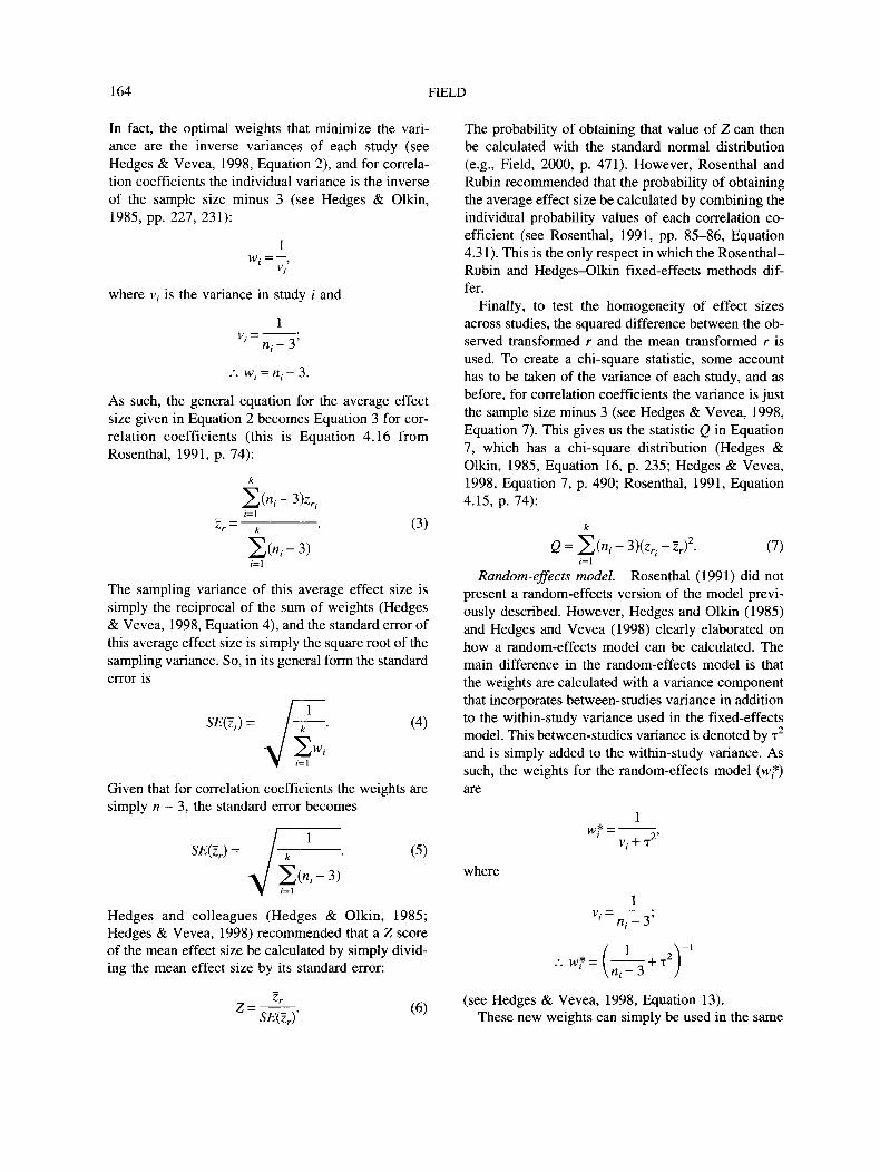
In fact, the optimal weights that minimize the vari-ance are the inverse variances of each study (seeHedges & Vevea, 1998, Equation 2), and for correla-tion coefficients the individual variance is the inverseof the sample size minus 3 (see Hedges & Olkin,1985, pp. 227, 231):
1
where v, is the variance in study i and
1
"'• n,-3'
/. wt = n( - 3.
As such, the general equation for the average effectsize given in Equation 2 becomes Equation 3 for cor-relation coefficients (this is Equation 4.16 fromRosenthal, 1991, p. 74):
Zr = - (3)
The sampling variance of this average effect size issimply the reciprocal of the sum of weights (Hedges& Vevea, 1998, Equation 4), and the standard error ofthis average effect size is simply the square root of thesampling variance. So, in its general form the standarderror is
(4)
Given that for correlation coefficients the weights aresimply n - 3, the standard error becomes
SE(zr) = (5)
Hedges and colleagues (Hedges & Olkin, 1985;Hedges & Vevea, 1998) recommended that a Z scoreof the mean effect size be calculated by simply divid-ing the mean effect size by its standard error:
The probability of obtaining that value of Z can thenbe calculated with the standard normal distribution(e.g., Field, 2000, p. 471). However, Rosenthal andRubin recommended that the probability of obtainingthe average effect size be calculated by combining theindividual probability values of each correlation co-efficient (see Rosenthal, 1991, pp. 85-86, Equation4.31). This is the only respect in which the Rosenthal-Rubin and Hedges-Olkin fixed-effects methods dif-fer.
Finally, to test the homogeneity of effect sizesacross studies, the squared difference between the ob-served transformed r and the mean transformed r isused. To create a chi-square statistic, some accounthas to be taken of the variance of each study, and asbefore, for correlation coefficients the variance is justthe sample size minus 3 (see Hedges & Vevea, 1998,Equation 7). This gives us the statistic Q in Equation7, which has a chi-square distribution (Hedges &Olkin, 1985, Equation 16, p. 235; Hedges & Vevea,1998, Equation 7, p. 490; Rosenthal, 1991, Equation4.15, p. 74):
k
i=l
Random-effects model. Rosenthal (1991) did notpresent a random-effects version of the model previ-ously described. However, Hedges and Olkin (1985)and Hedges and Vevea (1998) clearly elaborated onhow a random-effects model can be calculated. Themain difference in the random-effects model is thatthe weights are calculated with a variance componentthat incorporates between-studies variance in additionto the within-study variance used in the fixed-effectsmodel. This between-studies variance is denoted by T2
and is simply added to the within-study variance. Assuch, the weights for the random-effects model (w?)are
1
where
;.wf = + T
Z = (6)(see Hedges & Vevea, 1998, Equation 13).
These new weights can simply be used in the same
META-ANALYSIS OF CORRELATION COEFFICIENTS 165
way as for the fixed-effects model to calculate themean effect size, its standard error, and the z scoreassociated with it (by replacing the old weights withthe new weights in Equations 2, 4, and 6).
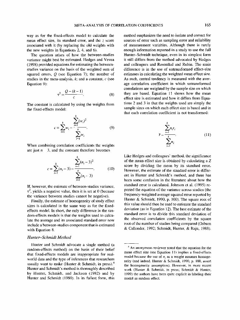
The question arises of how the between-studiesvariance might best be estimated. Hedges and Vevea(1998) provided equations for estimating the between-studies variance on the basis of the weighted sum ofsquared errors, Q (see Equation 7); the number ofstudies in the meta-analysis, k; and a constant, c (seeEquation 9):
(8)
The constant is calculated by using the weights fromthe fixed-effects model:
c = (9)
method emphasizes the need to isolate and correct forsources of error such as sampling error and reliabilityof measurement variables. Although there is rarelyenough information reported in a study to use the fullHunter-Schmidt technique, even in its simplest formit still differs from the method advocated by Hedgesand colleagues and Rosenthal and Rubin. The maindifference is in the use of untransformed effect-sizeestimates in calculating the weighted mean effect size.As such, central tendency is measured with the aver-age correlation coefficient in which untransformedcorrelations are weighted by the sample size on whichthey are based. Equation 11 shows how the meaneffect size is estimated and how it differs from Equa-tions 2 and 3 in that the weights used are simply thesample sizes on which each effect size is based and inthat each correlation coefficient is not transformed:
r — - (11)When combining correlation coefficients the weightsare just n - 3, and the constant therefore becomes
c = (10)
If, however, the estimate of between-studies variance,T2, yields a negative value, then it is set at 0 (becausethe variance between studies cannot be negative).
Finally, the estimate of homogeneity of study effectsizes is calculated in the same way as for the fixed-effects model. In short, the only difference in the ran-dom-effects models is that the weights used to calcu-late the average and its associated standard error nowinclude a between-studies component that is estimatedwith Equation 8.
Hunter—Schmidt Method
Hunter and Schmidt advocate a single method (arandom-effects method) on the basis of their beliefthat fixed-effects models are inappropriate for real-world data and the type of inferences that researchersusually want to make (Hunter & Schmidt, in press).4
Hunter and Schmidt's method is thoroughly describedby Hunter, Schmidt, and Jackson (1982) and byHunter and Schmidt (1990). In its fullest form, this
Like Hedges and colleagues' method, the significanceof the mean effect size is obtained by calculating a Zscore by dividing the mean by its standard error.However, the estimate of the standard error is differ-ent in Hunter and Schmidt's method, and there hasbeen some confusion in the literature about how thestandard error is calculated. Johnson et al. (1995) re-ported the equation of the variance across studies (thefrequency-weighted average squared error reported byHunter & Schmidt, 1990, p. 100). The square root ofthis value should then be used to estimate the standarddeviation (as in Equation 12). The best estimate of thestandard error is to divide this standard deviation ofthe observed correlation coefficients by the squareroot of the number of studies being compared (Osburn& Callender, 1992; Schmidt, Hunter, & Raju, 1988).
4 An anonymous reviewer noted that the equation for themean effect size (see Equation 11) implies a fixed-effectsmodel because the use of n, as a weight assumes homoge-neity (and indeed, Hunter & Schmidt, 1990, p. 100, assertthe homogeneity assumption). However, in more recentwork (Hunter & Schmidt, in press; Schmidt & Hunter,1999) the authors have been quite explicit in labeling theirmodel as random effect.
166 FIELD
Therefore, as Schmidt and Hunter (1999) have sub-sequently noted, the equation of the standard devia-tion used by Johnson et al. should be further dividedby the square root of the number of studies beingassimilated. Equations 12 and 13 show the correctversion (according to Schmidt & Hunter, 1999) of thestandard deviation of the mean and the calculation ofthe standard error. The Z score is calculated simply bydividing the mean effect size by the standard error ofthat mean (see Equation 14):
SD =
SD
""V?
z=SET'
(12)
(13)
(14)
In terms of homogeneity of effect sizes, again a chi-square statistic is calculated on the basis of the sum ofsquared errors of the mean effect size (see Hunter &Schmidt, 1990, pp. 110-112). Equation 15 shows howthe chi-square statistic is calculated from the samplesize on which the correlation is based (n), the squarederrors between each effect size and the mean, and thevariance:
x2 =(1-r2)2
(15)
Comparison of the Methods
There are two major differences between the meth-ods described. The first difference is the use of trans-formed or untransformed correlation coefficients. TheFisher transformation is typically used to eliminate aslight bias in the untransformed correlation coeffi-cient: The transformation corrects for a skew in thesampling distribution of rs that occurs as the popula-tion value of r becomes further from zero (see Fisher,1928). Despite the theoretical basis for this transfor-mation, Hunter and Schmidt (1990) have long advo-cated the use of untransformed correlation coeffi-cients, using theoretical arguments to demonstratebiases arising from Fisher's transformation (seeHunter, Schmidt, & Coggin, 1996). Hunter andSchmidt (1990) note that "the Fisher Z replaces a
small underestimation or negative bias by a typicallysmall overestimation, or positive bias, a bias that isalways greater in absolute value than the bias in theuntransformed correlation" (p. 102; see also Field,1999; Hunter et al., 1996; Schmidt, Gast-Rosenberg,& Hunter, 1980; Schmidt, Hunter, & Raju, 1988).
Some empirical evidence does suggest that trans-forming the correlation coefficient can be beneficial.Silver and Dunlap (1987) claimed that meta-analysisbased on Fisher-transformed correlations is alwaysless biased than when untransformed correlations areused. However, Strube (1988) noted that Silver andDunlap had incorrectly ignored the effect of the num-ber of studies in the analysis and so had based theirfindings on only a small number of studies. Strube(1988) showed that as the number of studies in-creased, the overestimation of effect sizes based onFisher-transformed correlations was almost exactlyequal in absolute terms to the underestimation of ef-fect sizes found when untransformed rs were used.Strube's data indicated that the bias in effect size es-timates based on transformed correlations was lessthan the bias in those based on untransformed corre-lations only when three or fewer studies were in-cluded in the meta-analysis (and even then only whenthese studies had sample sizes of 20 or less). It wouldbe the exception that actual meta-analytic reviewswould be based on such a small number of studies. Asa final point, Hunter et al. (1996) have argued thatwhen population correlations are the same for studiesin the meta-analysis (the homogeneous case) then re-sults based on transformed correlations should bewithin rounding error of those based on untrans-formed values.
The second difference is in the equations used toestimate the standard error. If we compare the ran-dom-effects model described by Hedges and Vevea(1998) to Hunter and Schmidt's, the estimates of stan-dard error are quite different. Hedges and Vevea havesuggested that Hunter and Schmidt "advocate the useof suboptimal weights that correspond to the fixed-effects weights, presumably because they assume thatT2 [the between-studies variance] is small" (p. 493).Therefore, if the between-studies variance is notsmall, the Hunter and Schmidt method will underes-timate the standard error and hence will overestimatethe z score associated with the mean (Hedges & Vevea,1998). However, Hedges and Vevea's estimate of thebetween-studies variance is truncated (because nega-tive values lead to the assumption that T2 = 0); sowhen there are only a small number of studies in
META-ANALYSIS OF CORRELATION COEFFICIENTS 167
the meta-analysis the estimate of between-studiesvariance will be biased, and the weights used to cal-culate the average effect size (and its significance)will also be biased.
Johnson et al. (1995) used a single database to com-pare the Hedges-Olkin (fixed-effects), Rosenthal-Rubin, and Hunter-Schmidt meta-analytic methods.By manipulating the characteristics of this database,Johnson et al. looked at the effects of the number ofstudies compared, the mean effect size of studies, themean number of participants per study, and the rangeof effect sizes within the database. In terms of theoutcomes of each meta-analysis, they looked at theresulting mean effect size, the significance of this ef-fect size, homogeneity of effect sizes, and predictionof effect sizes by a moderator variable. Their resultsshowed convergence of the methods in terms of themean effect size and estimates of the heterogeneity ofeffect sizes. However, the significance of the meaneffect size differed substantially across meta-analyticmethods. Specifically, the Hunter and Schmidtmethod seemed to reach more conservative estimatesof significance (and hence wider confidence intervals)than the other two methods. Johnson et al. concludedthat Hunter and Schmidt's method should be usedonly with caution.
Johnson et al.'s study (1995) provides some of theonly comparative evidence to suggest that some meta-analytic methods for combining correlations shouldbe preferred over others (although Overton, 1998, hasinvestigated moderator-variable effects across meth-ods); however, although their study clearly providedan excellent starting point at which to compare meth-ods, there were some limitations. First, Schmidt andHunter (1999) have criticized Johnson et al.'s work ata theoretical level, claiming that the wrong estimate ofthe standard error of the mean effect size was used intheir calculation of its significance. Schmidt andHunter went on to show that when a corrected esti-mate was used, estimates of the significance of themean effect size should be comparable to the Hedgesand Olkin and Rosenthal and Rubin methods. There-fore—-theoretically—the methods should yield com-parable results. Second, Johnson et al. applied Hedgesand Olkin's method for d (by first converting eachcorrelation coefficient from r to d). Hedges and Olkin(and Hedges & Vevea, 1998) provided methods fordirectly combining rs (without converting to d), andso this procedure did not represent what researcherswould actually do. Finally, the circumstances underwhich the three procedures were compared were lim-
ited to a single database that was manipulated toachieve the desired changes in the independent vari-ables of interest. This creates two concerns: (a) Theconclusions drawn might be a product of the proper-ties of the data set used (because, e.g., adding or sub-tracting a fixed integer from each effect size allowedJohnson et al. to look at situations in which the meaneffect size was higher or lower than in the originaldatabase; however, the relative strength of each effectsize remained constant throughout) and (b) the dataset assumed a fixed population effect size and so nocomparisons were made between random-effectsmodels. A follow-up study is needed in which MonteCarlo data simulations are used to expand Johnson etal.'s work.
Rationale and Predictions
Having reviewed the procedures to be compared,we can make some predictions about their relativeperformance. Although there has been much theoret-ical debate over the efficacy of the meta-analyticmethods (see Hedges & Vevea, 1998; Hunter &Schmidt, in press; Johnson et al., 1995; Schmidt &Hunter, 1999), in this study we aimed to test the ar-guments empirically. The rationale is that in meta-analysis, researchers combine results from differentstudies to try to ascertain knowledge of the effect sizein the population. Therefore, if data are sampled froma population with a known effect size, we can assessthe accuracy of each method by comparing the sig-nificance of the mean effect size from each methodagainst the known effect in the population. In the nullcase (population effect size p = 0) we expect to findnonsignificant results from each meta-analysis. To beprecise, with the nominal Type I error rate set at a =.05 the expectation is that only 5% of mean effectsizes should be significant. With the population effectsize set above zero the proportion of mean effect sizesthat are significant represents the power of eachmethod (assuming that the Type I error is controlled).
A number of predictions can be made on the basisof the arguments within the literature:
Prediction 1: On the basis of Hunter et al. (1996) andHunter and Schmidt (1990), it is pre-dicted that methods incorporating trans-formed effect-size estimates shouldshow an upward bias in their estimatesof the mean effect size. This biasshould be relatively small when popu-lation effect sizes are fixed (homoge-
168 FIELD
neous case) but larger when populationeffect sizes are variable (the heteroge-neous case).
Prediction 2: As the population value of r becomesfurther from zero, the sampling distri-bution of rs becomes skewed and Fish-er's transformation is used to normalizethis sampling distribution. Therefore,theoretically Hunter and Schmidt'smethod should become less accurate asthe effect size in the population in-creases (especially for small samplesizes). Conversely, techniques based onFisher's transformation should becomemore accurate with larger effect sizes inthe population. However, Strube (1988)and Hunter et al. (1996) have shownequivalent but opposite biases in meth-ods based on transformed and untrans-formed correlation coefficients whenmore than a few studies are included inthe meta-analysis. We expected the cur-rent study would replicate these laterfindings.
Prediction 3: Contrary to Johnson et al. (1995) find-ing that Hunter and Schmidt's methodyields conservative estimates of the sig-nificance of the mean effect size, wepredicted that estimates of significancewould be comparable across methods(because the present study was basedon the corrected formulas reported bySchmidt & Hunter, 1999).
Prediction 4: The estimates of between-studies vari-ance in Hedges and colleagues' ran-dom-effects model are biased for smallnumbers of studies. As such, it is pre-dicted that this method will be less ac-curate when only small numbers ofstudies are included in the meta-analysis.
Study 1: The Homogeneous Case
Two Monte Carlo studies were conducted to inves-tigate the effect of various factors on the average ef-fect size, the corresponding significance value, andthe homogeneity of effect-size tests. The first studylooked at the homogeneous case, and the second theheterogeneous case. In both studies the general ap-proach was the same: (a) A pseudopopulation was
created in which the effect size was known (homoge-neous case) or in which the population effect size wassampled from a normal distribution of effect sizeswith a known average (heterogeneous case); (b)samples of various sizes were taken from that popu-lation and the correlation coefficient calculated andstored (these samples can be thought of as studies ina meta-analysis); (c) when a specified number of thesestudies had been taken, different meta-analytic tech-niques were applied (for each technique, average ef-fect size, the Z value, and test of homogeneity werecalculated); and (d) the techniques were compared tosee the effect of the number of studies in the meta-analysis, and the relative size of those studies. Each ofthese steps is discussed immediately below in moredetail.
Method
Both studies were run using GAUSS for Windows3.2.35 (1998). In the homogeneous case, a pseudo-population was set up in which there was a knowneffect size (correlation between variables). This wasachieved by using the A matrix procedure describedby Mooney (1997), in which the correlation betweentwo randomly generated, normally distributed vari-ables is set using the Choleski decomposition of afixed-correlation matrix. Five different pseudopopu-lations were used in all: those in which there was noeffect (p = 0), a small effect size (p = .1), a moderateeffect size (p = .3), a large effect size (p = .5), anda very large effect (p = .8). These effect sizes werebased on Cohen's (1988, 1992) guidelines for a small,medium, and large effect (in terms of correlation co-efficients). For each Monte Carlo trial a set number ofstudies was taken from a given pseudopopulation, andaverage effect sizes and measures of homogeneity ofeffect sizes calculated. The Type I error rate or testpower were estimated from the proportion of signifi-cant results over 100,000 Monte Carlo trials.
Number of studies. The first factor in the MonteCarlo study was the number of studies used in themeta-analysis. This factor varied systematically from5 to 30 studies5 in increments of 5. Therefore, for thefirst set of Monte Carlo trials, the program took 5random studies from the pseudopopulation on each
5 The number of studies in real meta-analytic studies islikely to exceed 30 and would rarely be as small as 5;nevertheless, these values are fairly typical of moderatoranalysis in meta-analysis.
META-ANALYSIS OF CORRELATION COEFFICIENTS 169
trial. The correlation coefficients of the studies wereused to calculate the mean effect size (and other sta-tistics) by using each of the methods described. Theprogram stored the mean effect size, and a counterwas triggered if the average effect size was significant(based on the associated z score). A second counterwas triggered if the test of homogeneity was signifi-cant. Having completed this task, the next trial wasrun until 100,000 Monte Carlo trials were completed,after which the program saved the information, resetthe counters, increased the number of studies in themeta-analysis by 5 (so the number of studies became10), and repeated the process. The program stoppedincrementing the number of studies once 30 studieswas reached.
Average sample size. The second factor to be var-ied was the average sample size of each study in themeta-analysis. This variable was manipulated to seewhether the three methods differed across differentsample sizes. In most real-life meta-analyses, studysample sizes will not be equal; so to model reality,sample sizes were drawn from a normal distributionof possible sample sizes, with the mean of this distri-bution being systematically varied. Thus, rather thanfixing the sample size at a constant value (e.g., 40),sample sizes were randomly taken from a distributionwith a fixed mean (in this case 40) and a standarddeviation of a quarter of the mean (in this case 10).For each Monte Carlo trial, the sample size associatedwith the resulting r was stored in a separate vector foruse in the meta-analysis calculations.
Values of the average sample size were set usingestimates of the sample size necessary to detect small,medium, and large effects in the population. Based onCohen (1988) the sample size needed to detect a smalleffect is 150, to detect a medium-size effect a sampleof about 50 is needed, and to detect a large effect asample size of 25 will suffice. As such, the originalaverage sample size was set at 20. Once the programhad completed all computations for this sample size,the sample size was multiplied by 2 (average n = 40)and the program looped through all calculationsagain. The average sample size was then multipliedby 2 again (average n = 80) and so on to a maximumaverage sample size of 160. These sample sizes arelogical because, ceteris paribus, the smallest averagesample size (20) is big enough for only a very largeeffect (p = .8) to be detected. The next sample size(40) should enable both a very large and a slightlysmaller effect (p = .5) to be detected. The nextsample size (80) should be sufficient to detect all
but the smallest effect sizes, and the largest samplesize (160) should detect all sizes of population effectsizes.
Design. The overall design was a four-factor 5(population effect size: 0, .1, .3, .5, .8) x 4 (averagesample size: 20, 40, 80, 160) x 6 (no. studies: 5, 10,15,20,25, 30) x 2 (method of analysis: Hedges-Olkinand Rosenthal-Rubin vs. Hunter-Schmidt) designwith the method of analysis as a repeated measure.For each level of population effect size there were 24combinations of the average sample size and numberof studies. For each of these combinations 100,000Monte Carlo trials were used (100 times as many asthe minimum recommended by Mooney, 1997), soeach cell of the design contained 100,000 cases ofdata. Therefore, 2,400,000 samples of data were simu-lated per population effect size, and 12 million in thewhole study.
Results
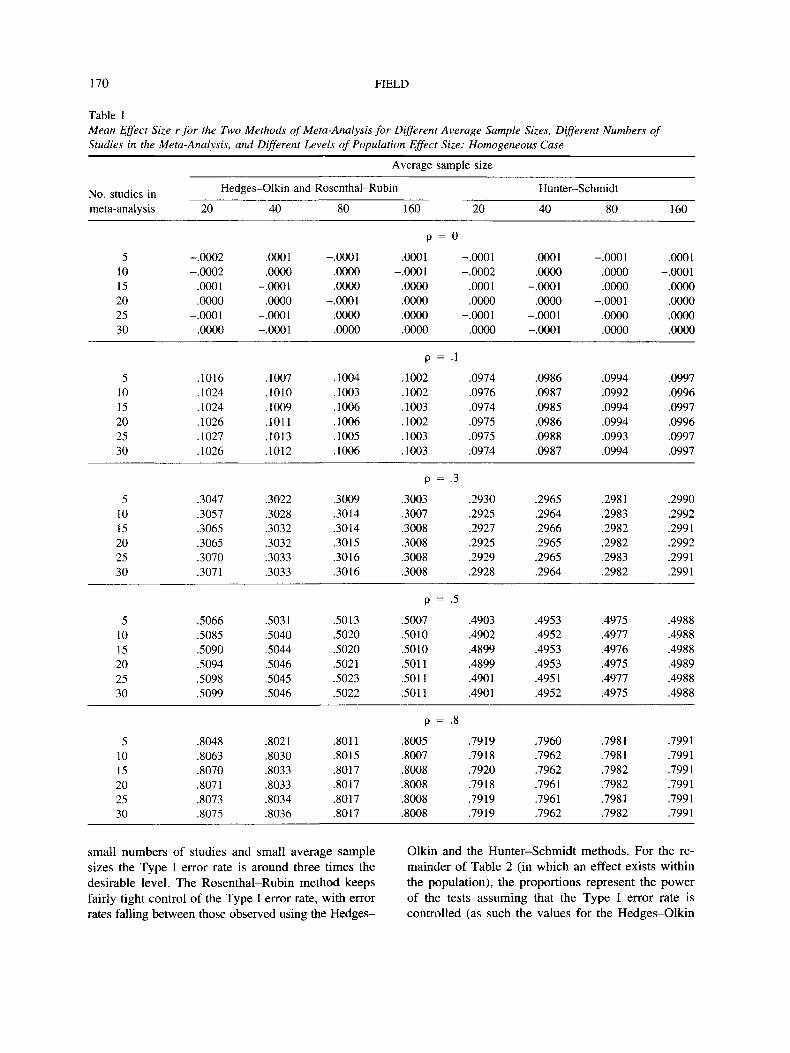
Mean effect sizes and their significance. Table 1shows the mean effect size from the two methodswhen the average sample size and number of samplesin the meta-analysis are varied. For the null case, allthree techniques produce accurate estimates of thepopulation effect size. As the effect size in the popu-lation increases, the Hedges-Olkin and Rosenthal-Rubin method tends to slightly overestimate the popu-lation effect size whereas the Hunter-Schmidt methodunderestimates it. This finding was predicted becausethese two methods differ in their use of transformedeffect-size estimates. The degree of bias appears to bevirtually identical when rounded to two decimalplaces.
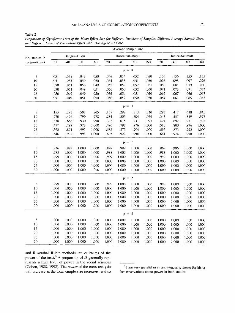
More interesting are the data presented in Table 2,which shows the proportion of significant results aris-ing from the Z score associated with the mean effectsize. This table also includes separate values for theRosenthal-Rubin method (because it differs from theHedges-Olkin method in terms of how significance isestablished). In the null case, these proportions rep-resent the Type I error rate for the three methods.Using a nominal a of .05, it is clear that the Hedges-Olkin method keeps tight control over the Type I errorrate (this finding supports data presented by Hedges &Vevea, 1998). The Hunter-Schmidt method does notcontrol the Type I error rate in the homogeneous case,although for a large total sample size (i.e., as thenumber of studies in the meta-analysis and the aver-age sample size of each study increases) the Type Ierror rate is better controlled (a = .06). However, for
170 FIELD
Table 1Mean Effect Size r for the Two Methods of Meta-Analysis for Different Average Sample Sizes, Different Numbers ofStudies in the Meta-Analysis, and Different Levels of Population Effect Size: Homogeneous Case
Average sample size
No. studies inmeta-analysis
51015202530
51015202530
51015202530
51015202530
51015202530
Hedges-Olkin and Rosenthal-Rubin
20
-.0002-.0002.0001.0000-.0001.0000
.1016
.1024
.1024
.1026
.1027
.1026
.3047
.3057
.3065
.3065
.3070
.3071
.5066
.5085
.5090
.5094
.5098
.5099
.8048
.8063
.8070
.8071
.8073
.8075
40
.0001
.0000-.0001.0000-.0001-.0001
.1007
.1010
.1009
.1011
.1013
.1012
.3022
.3028
.3032
.3032
.3033
.3033
.5031
.5040
.5044
.5046
.5045
.5046
.8021
.8030
.8033
.8033
.8034
.8036
80
-.0001.0000.0000
-.0001.0000.0000
.1004
.1003
.1006
.1006
.1005
.1006
.3009
.3014
.3014
.3015
.3016
.3016
.5013
.5020
.5020
.5021
.5023
.5022
.8011
.8015
.8017
.8017
.8017
.8017
160
P =
.0001-.0001.0000.0000.0000.0000
P =.1002.1002.1003.1002.1003.1003
P =
.3003
.3007
.3008
.3008
.3008
.3008
P =
.5007
.5010
.5010
.5011
.5011
.5011
P =
.8005
.8007
.8008
.8008
.8008
.8008
20
0
-.0001-.0002.0001.0000-.0001.0000
.1
.0974
.0976
.0974
.0975
.0975
.0974
.3
.2930
.2925
.2927
.2925
.2929
.2928
.5
.4903
.4902
.4899
.4899
.4901
.4901
.8
.7919
.7918
.7920
.7918
.7919
.7919
Hunter-Schmidt
40
.0001
.0000-.0001.0000-.0001-.0001
.0986
.0987
.0985
.0986
.0988
.0987
.2965
.2964
.2966
.2965
.2965
.2964
.4953
.4952
.4953
.4953
.4951
.4952
.7960
.7962
.7962
.7961
.7961
.7962
80
-.0001.0000.0000-.0001.0000.0000
.0994
.0992
.0994
.0994
.0993
.0994
.2981
.2983
.2982
.2982
.2983
.2982
.4975
.4977
.4976
.4975
.4977
.4975
.7981
.7981
.7982
.7982
.7981
.7982
160
.0001-.0001.0000.0000.0000.0000
.0997
.0996
.0997
.0996
.0997
.0997
.2990
.2992
.2991
.2992
.2991
.2991
.4988
.4988
.4988
.4989
.4988
.4988
.7991
.7991
.7991
.7991
.7991
.7991
small numbers of studies and small average samplesizes the Type I error rate is around three times thedesirable level. The Rosenthal-Rubin method keepsfairly tight control of the Type I error rate, with errorrates falling between those observed using the Hedges-
Olkin and the Hunter-Schmidt methods. For the re-mainder of Table 2 (in which an effect exists withinthe population), the proportions represent the powerof the tests assuming that the Type I error rate iscontrolled (as such the values for the Hedges-Olkin
META-ANALYSIS OF CORRELATION COEFFICIENTS 171
Table 2Proportion of Significant Tests of the Mean Effect Size for Different Numbers of Samples, Different Average Sample Sizes,and Different Levels of Population Effect Size: Homogeneous Case
Average sample size
No. studies inmeta-analysis
51015202530
51015202530
51015202530
51015202530
51015202530
Hedges-Olkin
20
.051
.051
.050
.050
.050
.051
.155
.270
.378
.477
.568
.646
.836
.985
.9991.0001.0001.000
.9991.0001.0001.0001.0001.000
1.0001.0001.0001.0001.0001.000
40
.051
.051
.051
.051
.049
.049
.282
.496
.666
.789
.871
.923
.9891.0001.0001.0001.0001.000
1.0001.0001.0001.0001.0001.000
1.0001.0001.0001.0001.0001.000
80
.049
.050
.050
.049
.049
.051
.508
.799
.930
.978
.993
.998
.0001.0001.0001.0001.0001.000
1.000.000.000.000.000.000
.000
.000
.000
.000
.000
.000
160
.050
.050
.049
.051
.050
.050
.805
.978
.9981.0001.0001.000
1.000.000.000.000.000.000
.000
.000
.000
.000
.000
.000
1.0001.0001.0001.0001.0001.000
20
.056
.054
.055
.056
.056
.056
.167
.284
.395
.496
.585
.665
.847
.988
.9991.0001.0001.000
.9991.0001.0001.0001.0001.000
1.0001.0001.0001.0001.0001.000
Rosenthal-Rubin
40
P =
.054
.053
.052
.050
.054
.052
P =
.288
.505
.675
.798
.873
.922
P =
.9891.0001.0001.0001.0001.000
P =
1.0001.0001.0001.0001.0001.000
P =1.0001.0001.0001.0001.0001.000
80
0
.052
.051
.052
.052
.051
.050
.1
.513
.804
.931
.976
.994
.998
.3
1.0001.0001.0001.0001.0001.000
.5
1.0001.0001.0001.0001.0001.000
.8
1.0001.0001.0001.0001.0001.000
160
.050
.050
.051
.050
.050
.050
.810
.979
.9971.0001.0001.000
1.0001.0001.0001.0001.0001.000
1.0001.0001.0001.0001.0001.000
.000
.000
.000
.000
.000
.000
20
.156
.098
.080
.071
.067
.064
.283
.343
.424
.510
.593
.661
.868
.983
.9991.0001.0001.000
.9981.0001.0001.0001.0001.000
1.0001.0001.0001.0001.0001.000
Hunter-Schmidt
40
.156
.098
.081
.073
.067
.063
.417
.557
.692
.800
.873
.924
.9861.0001.0001.0001.0001.000
1.0001.0001.0001.0001.0001.000
1.000.000.000.000.000.000
80
.153
.097
.079
.071
.066
.065
.618
.819
.931
.976
.992
.998
1.0001.0001.000.000
1.0001.000
1.000.000.000.000.000.000
1.000.000.000.000.000.000
160
.155
.096
.080
.073
.067
.063
.845
.977
.9981.0001.0001.000
1.0001.0001.0001.0001.0001.000
.000
.000
.000
.000
.000
.000
1.0001.0001.0001.0001.0001.000
and Rosenthal-Rubin methods are estimates of thepower of the test).6 A proportion of .8 generally rep-resents a high level of power in the social sciences(Cohen, 1988, 1992). The power of the meta-analysiswill increase as the total sample size increases, and so
6 I am very grateful to an anonymous reviewer for his orher observations about power in both studies.
172 FIELD
as both the number of studies and their respectivesample sizes increase, we expect a concomitant in-crease in power. The methods advocated by Hedgesand Olkin and by Rosenthal and Rubin both yield highlevels of power (greater than .8), except when thepopulation effect size is small (p = .1) and the totalsample size is relatively small. For example, when thenumber of studies in the meta-analysis is small (five),a high level of power is achieved only when the av-erage study sample size is 160; similarly, regardlessof the number of studies, a high level of power is notachieved when the average study sample size is only20, and when the average sample size is 40 a highdegree of power is achieved only when there are morethan 20 studies. For all other population effect sizes (p> .1) the probability of detecting a genuine effect isgreater than .8. For the Hunter-Schmidt method,power estimations cannot be made because the TypeI error rate is not controlled; nevertheless, the valuesin Table 2 are comparable to those for the other twomethods.
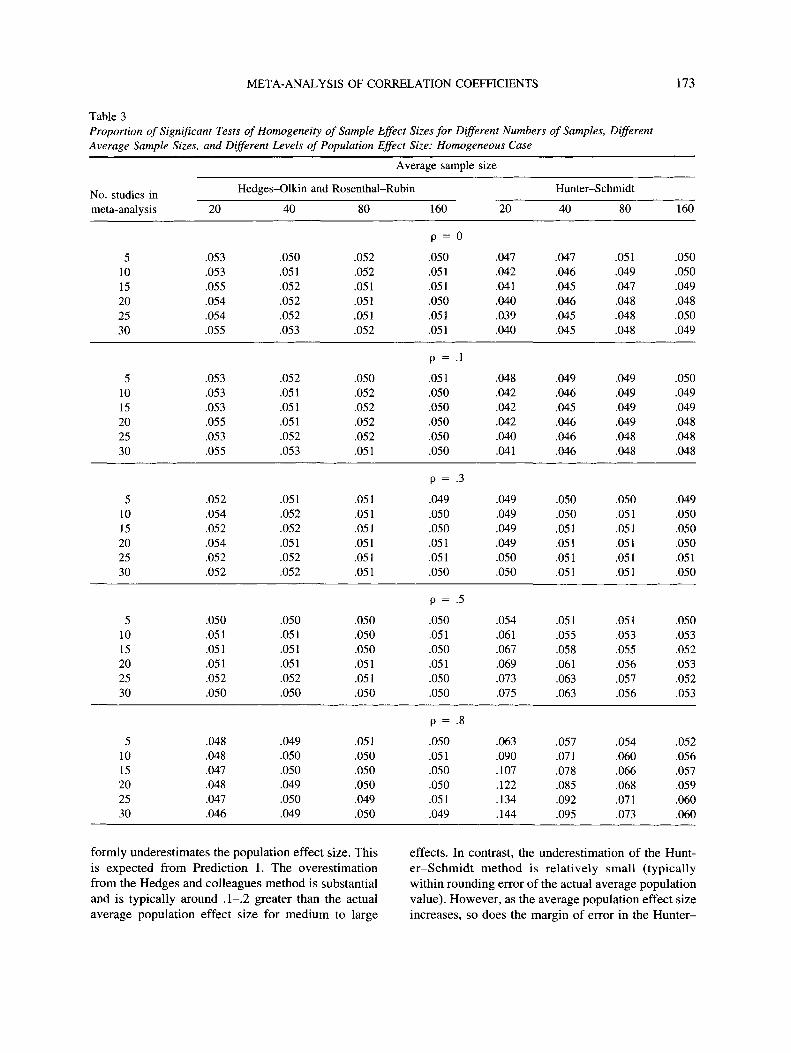
Tests of homogeneity of effect sizes. Table 3shows the proportion of significant tests of homoge-neity of effect sizes. In this study, the population ef-fect sizes were fixed (hence homogeneous); therefore,these tests of homogeneity should yield nonsignificantresults. The proportions in Table 3 should therefore beclose to the nominal a of .05. For small to mediumeffect sizes (p ̂ .3), both methods control the Type Ierror rate under virtually all conditions. For largerpopulation effect sizes (p > .5) the Hedges-Olkin andRosenthal-Rubin method controls the Type I errorrate to within rounding error of the nominal a. How-ever, the Hunter-Schmidt method begins to deviatesubstantially from the nominal a when the averagesample size is small (< 40), and this deviation in-creases as the number of studies within the meta-analysis increases. These results conform to acceptedstatistical theory (see Prediction 2 in the Rationale andPredictions section) in that the benefit of transformedeffect sizes is increasingly apparent as the populationeffect size increases.
Summary. To sum up, Study 1 empirically dem-onstrated several things: (a) Both meta-analytic meth-ods yield comparable estimates of population effectsizes; (b) the Type I error rates were well controlledfor the Hedges-Olkin and Rosenthal-Rubin methodsin all circumstances—however, the Hunter-Schmidtmethod seemed to produce liberal significance teststhat inflated the observed error rate above the nominala; (c) the Hedges-Olkin and Rosenthal-Rubin meth-
ods yielded power levels above .8 for medium andlarge effect sizes, but not for small effect sizes whenthe number of studies or average sample size wasrelatively small; (d) Type I error rates for tests ofhomogeneity of effect sizes were equally well con-trolled by the two methods when population effectsizes were small to medium, but better controlled bythe Hedges-Olkin and Rosenthal-Rubin methodwhen effect sizes were large.
Study 2: The Heterogeneous Case
Method
The method for the heterogeneous case was virtu-ally identical to that of the homogeneous case: Boththe number of studies and the average sample sizewere varied in the same systematic way. However, inthis study, population effect sizes were not fixed. Anormal distribution of possible effect sizes was cre-ated (a superpopulation) from which the populationeffect size for each study in a meta-analysis wassampled. As such, studies in a meta-analysis camefrom populations with different effect sizes. To lookat a variety of situations, the mean effect size of thesuperpopulation (p) was varied to be 0 (the null case),.1, .3, .5, and .8. The standard deviation of the super-population was set at .16 because (a) for a mediumpopulation effect size (p = .3) this represents a situ-ation in which 95% of population effect sizes will liebetween 0 (no effect) and .6 (strong effect), and (b)Barrick and Mount (1991) found this to be the stan-dard deviation of population correlations in a largemeta-analysis and so it represents a realistic estimateof the standard deviation of population correlations ofreal-world data (see Hunter & Schmidt, in press). Themethods used to combine correlation coefficients inthis study were the Hunter-Schmidt method andHedges and colleagues' random-effects model. As inStudy 1, 100,000 Monte Carlo trials were used foreach combination of average sample size, number ofstudies in the meta-analysis, and average populationeffect size.
Results
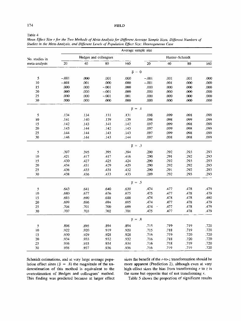
Mean effect sizes and their significance. Table 4shows the mean effect size from the two methodswhen the average sample size and number of studiesin the meta-analysis are varied. In the null case bothmethods produce accurate estimations of the popula-tion effect size. When there is an effect in the popu-lation, the Hedges and colleagues method uniformlyoverestimates and the Hunter-Schmidt method uni-
META-ANALYSIS OF CORRELATION COEFFICIENTS 173
Table 3Proportion of Significant Tests of Homogeneity of Sample Effect Sizes for Different Numbers of Samples, DifferentAverage Sample Sizes, and Different Levels of Population Effect Size: Homogeneous Case
Average sample size
No. studies inmeta-analysis
51015202530
51015202530
51015202530
51015202530
51015202530
Hedges-Olkin and Rosenthal-Rubin
20
.053
.053
.055
.054
.054
.055
.053
.053
.053
.055
.053
.055
.052
.054
.052
.054
.052
.052
.050
.051
.051
.051
.052
.050
.048
.048
.047
.048
.047
.046
40
.050
.051
.052
.052
.052
.053
.052
.051
.051
.051
.052
.053
.051
.052
.052
.051
.052
.052
.050
.051
.051
.051
.052
.050
.049
.050
.050
.049
.050
.049
80
.052
.052
.051
.051
.051
.052
.050
.052
.052
.052
.052
.051
.051
.051
.051
.051
.051
.051
.050
.050
.050
.051
.051
.050
.051
.050
.050
.050
.049
.050
160
p = 0
.050
.051
.051
.050
.051
.051
P = -I
.051
.050
.050
.050
.050
.050
p = .3
.049
.050
.050
.051
.051
.050
p = .5
.050
.051
.050
.051
.050
.050
p = .8
.050
.051
.050
.050
.051
.049
20
.047
.042
.041
.040
.039
.040
.048
.042
.042
.042
.040
.041
.049
.049
.049
.049
.050
.050
.054
.061
.067
.069
.073
.075
.063
.090
.107
.122
.134
.144
Hunter-Schmidt
40
.047
.046
.045
.046
.045
.045
.049
.046
.045
.046
.046
.046
.050
.050
.051
.051
.051
.051
.051
.055
.058
.061
.063
.063
.057
.071
.078
.085
.092
.095
80
.051
.049
.047
.048
.048
.048
.049
.049
.049
.049
.048
.048
.050
.051
.051
.051
.051
.051
.051
.053
.055
.056
.057
.056
.054
.060
.066
.068
.071
.073
160
.050
.050
.049
.048
.050
.049
.050
.049
.049
.048
.048
.048
.049
.050
.050
.050
.051
.050
.050
.053
.052
.053
.052
.053
.052
.056
.057
.059
.060
.060
formly underestimates the population effect size. Thisis expected from Prediction 1. The overestimationfrom the Hedges and colleagues method is substantialand is typically around .1-.2 greater than the actualaverage population effect size for medium to large
effects. In contrast, the underestimation of the Hunt-er-Schmidt method is relatively small (typicallywithin rounding error of the actual average populationvalue). However, as the average population effect sizeincreases, so does the margin of error in the Hunter-
174 FIELD
Table 4Mean Effect Size r for the Two Methods of Meta-Analysis for Different Average Sample Sizes, Different Numbers ofStudies in the Meta-Anatysis, and Different Levels of Population Effect Size: Heterogeneous Case
Average sample size
No. studies inmeta-analysis
51015202530
51015202530
51015202530
51015202530
51015202530
Hedges and colleagues
20
-.001-.001
.000
.000
.000
.000
.134
.141
.142
.143
.144
.146
.397
.421
.430
.434
.436
.438
.643
.680
.693
.699
.704
.707
.896
.922
.930
.934
.936
.938
40
.000
.001
.000
.000
.000
.000
.134
.140
.143
.144
.144
.144
.395
.417
.427
.431
.433
.436
.641
.677
.690
.696
.701
.703
.895
.920
.929
.933
.935
.937
80
.001
.000-.001-.001-.001
.000
.131
.139
.141
.142
.143
.143
.395
.417
.425
.429
.431
.433
.640
.676
.688
.694
.700
.702
.894
.919
.928
.932
.934
.936
160
p = 0
.000
.000
.000
.000
.001
.000
p = .1
.131
.139
.142
.143
.143
.144
p = .3
.394
.416
.424
.429
.432
.433
p = .5
.639
.675
.688
.695
.699
.701
p = .8
.894
.920
.928
.932
.934
.936
20
-.001-.001
.000
.000
.000
.000
.098
.098
.097
.097
.097
.097
.290
.290
.290
.290
.290
.289
.474
.475
.474
.474
.474 •
.475
.715
.715
.716
.716
.716
.716
Hunter-Schmidt
40
.001
.001
.000
.000
.000
.000
.099
.098
.099
.099
.099
.098
.292
.291
.292
.292
.291
.292
.477
.477
.478
.477
.477
.477
.719
.718
.719
.718
.718
.719
80
.001
.000
.000
.000
.000
.000
.098
.099
.098
.098
.098
.098
.293
.292
.293
.292
.292
.293
.478
.478
.478
.478
.478
.478
.719
.719
.720
.720
.719
.719
160
.000
.000
.000
.000
.000
.000
.099
.099
.099
.099
.099
.099
.293
.293
.293
.293
.293
.293
.479
.479
.480
.479
.479
.479
.720
.720
.720
.720
.720
.720
Schmidt estimations, and at very large average popu-lation effect sizes (p = .8) the magnitude of the un-derestimation of this method is equivalent to theoverestimation of Hedges and colleagues' method.This finding was predicted because at larger effect
sizes the benefit of the r-to-z transformation should bemore apparent (Prediction 2), although even at veryhigh effect sizes the bias from transforming r to z isthe same but opposite that of not transforming r.
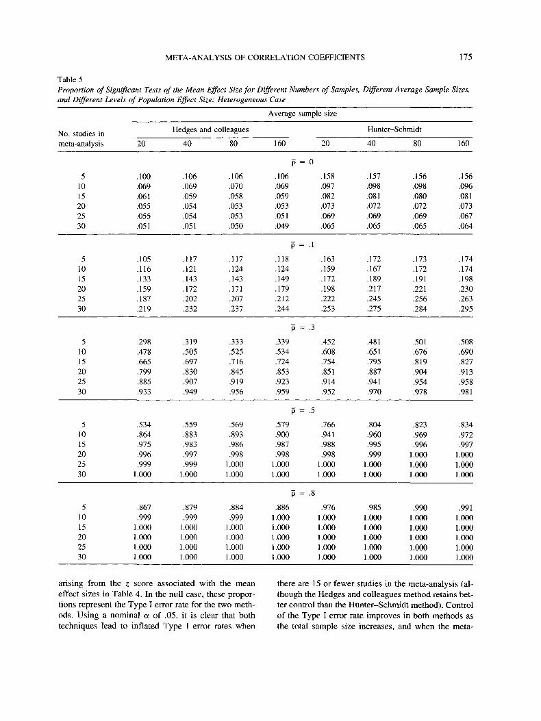
Table 5 shows the proportion of significant results
META-ANALYSIS OF CORRELATION COEFFICIENTS 175
Table 5Proportion of Significant Tests of the Mean Effect Size for Different Numbers of Samples, Different Average Sample Sizes,and Different Levels of Population Effect Size: Heterogeneous Case
Average sample size
No. studies inmeta-analysis
51015202530
51015202530
51015202530
51015202530
51015202530
20
.100
.069
.061
.055
.055
.051
.105
.116
.133
.159
.187
.219
.298
.478
.665
.799
.885
.933
.534
.864
.975
.996
.9991.000
.867
.9991.0001.0001.0001.000
Hedges and
40
.106
.069
.059
.054
.054
.051
.117
.121
.143
.172
.202
.232
.319
.505
.697
.830
.907
.949
.559
.883
.983
.997
.9991.000
.879
.9991.0001.0001.0001.000
colleagues
80
.106
.070
.058
.053
.053
.050
.117
.124
.143
.171
.207
.237
.333
.525
.716
.845
.919
.956
.569
.893
.986
.9981.0001.000
.884
.9991.0001.0001.0001.000
Hunter-Schmidt
160
P =
.106
.069
.059
.053
.051
.049
P =
.118
.124
.149
.179
.212
.244
P =
.339
.534
.724
.853
.923
.959
P =
.579
.900
.987
.9981.0001.000
P =
.8861.0001.0001.0001.0001.000
20
0
.158
.097
.082
.073
.069
.065
.1
.163
.159
.172
.198
.222
.253
.3
.452
.608
.754
.851
.914
.952
.5
.766
.941
.988
.9981.0001.000
.8
.9761.0001.0001.0001.0001.000
40
.157
.098
.081
.072
.069
.065
.172
.167
.189
.217
.245
.275
.481
.651
.795
.887
.941
.970
.804
.960
.995
.9991.0001.000
.9851.0001.0001.0001.0001.000
80
.156
.098
.080
.072
.069
.065
.173
.172
.191
.221
.256
.284
.501
.676
.819
.904
.954
.978
.823
.969
.9961.0001.0001.000
.9901.0001.0001.0001.0001.000
160
.156
.096
.081
.073
.067
.064
.174
.174
.198
.230
.263
.295
.508
.690
.827
.913
.958
.981
.834
.972
.9971.0001.0001.000
.9911.0001.0001.0001.0001.000
arising from the z score associated with the meaneffect sizes in Table 4. In the null case, these propor-tions represent the Type I error rate for the two meth-ods. Using a nominal a of .05, it is clear that bothtechniques lead to inflated Type I error rates when
there are 15 or fewer studies in the meta-analysis (al-though the Hedges and colleagues method retains bet-ter control than the Hunter-Schmidt method). Controlof the Type I error rate improves in both methods asthe total sample size increases, and when the meta-
176 FIELD
analysis includes a large number of studies (30),Hedges and colleagues' method produces error rateswithin rounding distance of the nominal a level. Evenfor large numbers of studies, the Hunter-Schmidtmethod inflates the Type 1 error rate.
For the remainder of the table (in which an effectexists within the population), the proportions dis-played represent the power of the tests assuming thatthe Type I error rate is controlled. Given that neithermethod has absolute control over the Type I error rate,these values need to be interpreted cautiously. What isclear is that the two methods yield very similar re-sults: For a small average population effect size (p =. 1) the probability of detecting an effect is under .3 forboth methods. High probabilities of detecting an ef-fect (>.8) are achieved only for large average popu-lation effect sizes (p S: .5) or for medium effect sizes(p = .3) when there is a relatively large number ofsamples (20 or more). The only substantive discrep-ancy between the methods is that the values forHedges and colleagues' method are lower when thereare only five studies in the meta-analysis, which waspredicted (Prediction 4). This difference is negligiblewhen the average population effect size is very large(P = .8).
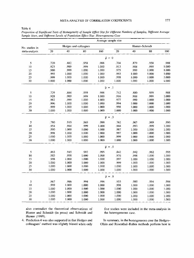
Tests of homogeneity of effect sizes. Table 6shows the proportion of significant tests of homoge-neity of effect sizes. In this study, the population ef-fect sizes were heterogeneous; therefore, these testsshould yield significant results. The proportions inTable 6, therefore, represent the power of the tests todetect variability in effect sizes assuming that theType I error rate is controlled. This study does notpresent data to confirm that the methods control theType I error rate (which would require that these testsbe applied to the homogeneous case); nevertheless,for all average population effect sizes the two meth-ods yield probabilities of detecting an effect greaterthan .8 with samples of 40 or more regardless of thenumber of studies in the meta-analysis. Even at smallsample sizes and numbers of studies, the proportion oftests that correctly detected genuine variance betweenpopulation parameters is close to .8 (the lowest prob-ability being .704) and comparable between methods.
Summary. Study 2 empirically demonstrated sev-eral interesting findings: (a) The Hunter-Schmidtmethod produces the most accurate estimates of popu-lation effect sizes when population effect sizes arevariable, but the benefit of this method is lost whenthe average population effect size is very large (p =.8); (b) the Type I error rates were not controlled by
either method when 15 or fewer studies were includedin the meta-analysis (although the Hedges-Olkinmethod was better in this respect)—however, as thetotal sample size increased, the Type I error rate wasbetter controlled for both methods; (c) althoughflawed by the lack of control of the Type I error rate,the potential power of both techniques was less than.3 when the average population effect size was small;(d) for large average population effect sizes the threetechniques were comparable for probable test power,but for small numbers of studies in the meta-analysis,Hedges and colleagues' method yielded lower powerestimates; and (e) power rates for tests of homogene-ity of effect sizes were comparable for both tech-niques in all circumstances.
Conclusion
This study presents the results of a thorough simu-lation of conditions that might influence the efficacyof different methods of meta-analysis. In an attempt todevelop Johnson et al.'s (1995) work, this study usedMonte Carlo simulation rather than manipulation of asingle data set. In doing so, these data provide abroader insight into the behavior of different meta-analytic procedures in an applied context (rather thanthe theoretical context of Hunter & Schmidt, in press;Schmidt & Hunter, 1999). Several predictions weresupported:
1. Prediction 1 was substantiated in that the Hedges-Olkin and Rosenthal-Rubin methods (using trans-formed effect-size estimates) led to upward biasesin effect-size estimates. These biases were negli-gible in the homogeneous case but substantial inthe heterogeneous case.
2. Prediction 2 was also substantiated with the Hunt-er-Schmidt method underestimating population ef-fect sizes. This bias increased as the populationeffect sizes increased (as predicted). However, thisbias was negligible in the homogeneous case andwas less severe than the Hedges-Olkin method inthe heterogeneous case.
3. Results for Prediction 3 were complex. TheHedges-Olkin method best controlled the Type Ierror rate, and the Hunter-Schmidt method led tothe greatest deviations from the nominal a. How-ever, unlike Johnson et al. (1995), who found thatthe Hunter-Schmidt method was too conservative,this study showed that the Hunter-Schmidt method(using their revised formula) was too liberal—toomany null results were significant. These results
META-ANALYSIS OF CORRELATION COEFFICIENTS 177
Table 6Proportion of Significant Tests of Homogeneity of Sample Effect Size for Different Numbers of Samples, Different AverageSample Sizes, and Different Levels of Population Effect Size: Heterogeneous Case
Average sample size
No. studies inmeta-analysis
51015202530
51015202530
51015202530
51015202530
51015202530
20
.720
.925
.980
.995
.9991.000
.729
.928
.982
.996
.9991.000
.780
.954
.990
.9981.0001.000
.863
.983
.9981.0001.0001.000
.967
.9991.0001.0001.0001.000
Hedges and
40
.882
.989
.9991.0001.0001.000
.884
.989
.9991.0001.0001.000
.910
.9941.0001.0001.0001.000
.945
.9981.0001.0001.0001.000
.9861.0001.0001.0001.0001.000
colleagues
80
.958
.9991.0001.0001.0001.000
.959
.9991.0001.0001.0001.000
.969
.9991.0001.0001.0001.000
.9821.0001.0001.0001.0001.000
.9941.0001.0001.0001.0001.000
Hunter-Schmidt
160
P =
.9881.0001.0001.0001.0001.000
P ~
.9881.0001.0001.0001.0001.000
P =
.9901.0001.0001.0001.0001.000
P =
.9951.0001.0001.0001.0001.000
P =
.9961.0001.0001.0001.0001.000
20
0
.704
.913
.975
.993
.9981.000
.1
.712
.916
.977
.994
.9981.000
.3
.762
.944
.987
.997
.9991.000
.5
.842
.976
.997
.9991.0001.000
.8
.953
.9981.0001.0001.0001.000
40
.879
.988
.9991.0001.0001.000
.880
.988
.9991.0001.0001.000
.907
.9931.0001.0001.0001.000
.942
.9981.0001.0001.0001.000
.985
.000
.000
.000
.000
.000
80
.958
.9991.0001.0001.0001.000
.959
.9991.0001.0001.0001.000
.969
.9991.0001.0001.0001.000
.9821.0001.0001.0001.0001.000
.9941.0001.0001.0001.0001.000
160
.988
.000
.000
.000
.000
.000
.9881.0001.0001.0001.0001.000
.9901.0001.0001.0001.0001.000
.9951.0001.0001.0001.0001.000
.996
.000
.000
.000
.000
.000
also contradict the theoretical observations ofHunter and Schmidt (in press) and Schmidt andHunter (1999).
4. Prediction 4 was also supported in that Hedges andcolleagues' method was slightly biased when only
five studies were included in the meta-analysis inthe heterogeneous case.
In summary, in the homogeneous case the Hedges-Olkin and Rosenthal-Rubin methods perform best in
178 FIELD
terms of significance tests of the average effect size:Contrary to Johnson et al. (1995), the present resultsindicate that the Hunter-Schmidt method is too liberalin the homogeneous case (not too conservative), butthis means that the method should, nevertheless, beapplied with caution in these circumstances. In termsof estimates of effect size and homogeneity of effect-size tests there are few differences between theHedges-Olkin and Rosenthal-Rubin methods and thatof Hunter and Schmidt. In the heterogeneous case, theHunter-Schmidt method yields the most accurate es-timates of population effect size across a variety ofsituations. The most surprising result was that neitherthe Hunter-Schmidt nor the Hedges and colleaguesmethod controlled the Type I error rate in the hetero-geneous case when 15 or fewer studies were includedin the meta-analysis. As such, in the heterogeneouscase researchers cannot be confident about the teststhey use unless the number of studies being combined(and hence the total sample size) is very large (at least30 studies in the meta-analysis for Hedges and col-leagues' method and more for the Hunter-Schmidtmethod). In addition, the probabilities of detecting asmall effect in the heterogeneous case were verysmall, and for medium effect sizes they were smallwhen 10 or fewer studies were in the meta-analysis.Given that the heterogeneous case is more represen-tative of real-world data (National Research Council,1992; Osburn & Callender, 1992), the implication isthat meta-analytic methods for combining correlationcoefficients may be relatively insensitive to detectingsmall effects in the population. As such, genuine ef-fects may be overlooked. However, this conclusionmust be qualified: When 15 or fewer studies are in-cluded in the meta-analysis, neither random-effectsmodel controls the Type I error rate as such accuratepower levels cannot be estimated. As such, the findingthat the probabilities of detecting medium populationeffect sizes (p = .3) are low for fewer than 15 studiesis, at best, tentative. Nevertheless, for small popula-tion effect sizes (p = .1), even when Type I errorrates are controlled (the Hedges and colleaguesmethod when 20 or more studies are included in themeta-analysis) the power of the random-effects modelis relatively small (average power across all factors is.209).
Using Meta-Analysis for Correlations
There are many considerations when applying tech-niques to combine correlation coefficients. The first iswhether the researcher wishes to make conditional or
unconditional inferences from the meta-analysis, or inother terms, whether the researcher wishes to assumethat the population effect size is fixed or variable. Asalready mentioned, it is more often the case that popu-lation effect sizes are variable (National ResearchCouncil, 1992; Osburn & Callender, 1992) and thatthe assumption of fixed population effect sizes is ten-able only if a researcher does not wish to generalizebeyond the set of studies within a meta-analysis(Hedges & Vevea, 1998; Hunter & Schmidt, in press).One practical way to assess whether population effectsizes are likely to be fixed or variable is to use thetests of homogeneity of study effect sizes associatedwith the three methods of meta-analysis. If this test isnonsignificant then it can be argued that populationeffect sizes are also likely to be homogeneous (andhence fixed to some extent). However, these teststypically have low power to detect genuine variationin population effect sizes (Hedges & Olkin, 1985;National Research Council, 1992), and so they canlead researchers to conclude erroneously that popula-tion effect sizes are fixed. The present data suggestthat the test of homogeneity of effect sizes advocatedby Hedges and Olkin and Rosenthal and Rubin andthe method suggested by Hunter and Schmidt haverelatively good control of Type I errors when effectsizes are, in reality, fixed. When effect sizes are vari-able in reality, both Hedges and colleagues' methodand the Hunter-Schmidt method produce equivalentestimates of power (although when the average effectsize is large and the average sample size is less than40 the Hunter-Schmidt method loses control of theType I error rate). However, in this latter case thesedetection rates are difficult to interpret because thereare no simulations in the current study to test whetherthe random-effects homogeneity tests control theType I error rate in the fixed case (when populationeffect sizes are, in reality, the same across studies).
The second issue is whether the researcher wishesto accurately estimate the population effect size oraccurately test its significance. In the homogeneouscase, all methods yield very similar estimates of thepopulation effect size. However, in the heterogeneouscase the Hunter-Schmidt method produces more ac-curate estimates, except when the average populationeffect size is very large (p = .8). In terms of testingthe significance of this estimate, Hedges and col-leagues' method keeps the best control over Type Ierrors in both the homogeneous and heterogeneouscase; however, in the heterogeneous case neither thismethod nor the Hunter-Schmidt method actually con-
META-ANALYSIS OF CORRELATION COEFFICIENTS 179
trols the Type I error rate acceptably when fewer than15 studies are included in the meta-analysis.
Third, the researcher has to consider controlling forother sources of error. It is worth remembering thatsmall statistical differences in average effect size es-timates and the like may be relatively unimportantcompared with other forms of bias such as unreliabil-ity of measures. Hunter and Schmidt (1990) discussways in which these biases can be accounted for, andthe experienced meta-analyst should consider theseissues when deciding on a technique. The Hunter-Schmidt method used in the present article is only thesimplest form of this method and so does not reflectthe full method adequately. Despite its relative short-comings in the homogeneous case, the addition ofprocedures for controlling other sources of bias maymake this method very attractive in situations inwhich the researcher can estimate and control forthese other confounds. However, further research isneeded to test the accuracy of the adjustments forerror sources proposed by Hunter and Schmidt.
Final Remarks
This study has shown that the Hunter-Schmidtmethod tends to provide the most accurate estimatesof the mean population effect size when effect sizesare heterogeneous, which is the most common case inmeta-analytic practice. In the heterogeneous case,Hedges and colleagues' method tended to overesti-mate effect sizes by about 15%-45%, whereas theHunter-Schmidt method tended to underestimate it bya smaller amount (about 5%-10%), and then onlywhen the population average correlation exceeded .5.In terms of the Type I error rate for the significancetests associated with these estimates, Hedges and col-leagues' method does control this error rate in thehomogeneous case. The most surprising finding isthat neither random-effects method controls the TypeI error rate in the heterogeneous case (except when alarge number of studies are included in the meta-analysis)—although Hedges and colleagues' methodinflates the Type I error rate less than the Hunter-Schmidt method. Given that the National ResearchCouncil (1992) and others have suggested that theheterogeneous case is the rule rather than the excep-tion, this implies that estimates and significance testsfrom meta-analytic studies containing less than 30samples should be interpreted very cautiously. Eventhen, random-effects methods seem poor at detectingsmall population effect sizes. Further work should ex-amine the efficacy of other random-effects models of
meta-analysis such as multilevel modeling (Goldstein,1995; Goldstein, Yang, Omar, Turner, & Thompson,2000).
References
Barrick, M. R., & Mount, M. K. (1991). The Big Fivepersonality dimensions and job performance: A meta-analysis. Personnel Psychology, 44, 1-26.
Becker, B. J. (1996). The generalizability of empirical re-search results. In C. P. Benbow & D. Lubinski (Eds.),Intellectual talent: Psychological and social issues (pp.363-383). Baltimore: Johns Hopkins University Press.
Cohen, J. (1988). Statistical power analysis for the behav-ioural sciences (2nd ed.). New York: Academic Press.
Cohen, J. (1992). A power primer. Psychological Bulletin,112, 155-159.
Field, A. P. (1999). A bluffer's guide to meta-analysis: I.Correlations. Newsletter of the Mathematical, Statisticaland Computing Section of the British Psychological So-ciety, 7(1), 16-25.
Field, A. P. (2000). Discovering statistics using SPSS forWindows: Advanced techniques for the beginner. Lon-don: Sage.
Fisher, R. A. (1928). Statistical methods for research work-ers (2nd ed.). London: Oliver & Boyd.
GAUSS for Windows 3.2.35 [Computer software]. (1998).Maple Valley, WA: Aptech Systems.
Glass, G. (1976). Primary, secondary, and meta-analysis ofresearch. Educational Researcher, 51, 3-8.
Glass, G., McGaw, B., & Smith, M. L. (1981). Meta-analysis in social research. Beverly Hills, CA: Sage.
Goldstein, H. (1995). Multilevel statistical models. London:Edward Arnold.
Goldstein, H., Yang, M., Omar, R., Turner, R., & Thomp-son, S. (2000). Meta-analysis using multilevel modelswith an application to the study of class size effects.Journal of the Royal Statistical Society, Series C: AppliedStatistics, 49, 399^412.
Hedges, L. V. (1992). Meta-analysis. Journal of Education-al Statistics, 17, 279-296.
Hedges, L. V. (1994a). Fixed effects models. In H. Cooper& L. V. Hedges (Eds.), Handbook of research synthesis(pp. 285-300). New York: Russell Sage Foundation.
Hedges, L. V. (1994b). Statistical considerations. In H.Cooper & L. V. Hedges (Eds.), Handbook of researchsynthesis (pp. 29-38). New York: Russell Sage Founda-tion.
Hedges, L. V., & Olkin, I. (1985). Statistical methods formeta-analysis. Orlando, FL: Academic Press.
Hedges, L. V., & Vevea, J. L. (1998). Fixed- and random-
180 FIELD
effects models in meta-analysis. Psychological Methods,3, 486-504.
Hunter, J. E., & Schmidt, F. L. (1990). Methods of meta-analysis: Correcting error and bias in research findings.Newbury Park, CA: Sage.
Hunter, J. E., & Schmidt, F. L. (in press). Fixed effects vs.random effects meta-analysis models: Implications forcumulative knowledge in psychology. InternationalJournal of Selection and Assessment.
Hunter, J. E., Schmidt, F. L., & Coggin, T. D. (1996). Meta-analysis of correlations: Bias in the correlation coeffi-cient and the Fisher z transformation. Unpublishedmanuscript.
Hunter, J. E., Schmidt, F. L., & Jackson, G. B. (1982).Meta-analysis: Cumulating research findings acrossstudies. Beverly Hills, CA: Sage.
Johnson, B. T., Mullen, B., & Salas, E. (1995). Comparisonof three major meta-analytic approaches. Journal of Ap-plied Psychology, 80, 94-106.
Law, K. S., Schmidt, F. L., & Hunter, J. E. (1994). Non-linearity of range corrections in meta-analysis: Test of animproved procedure. Journal of Applied Psychology, 79,425-138.
Mooney, C. Z. (1997). Monte Carlo simulation [Sage Uni-versity Paper Series on Quantitative Applications in theSocial Sciences, 07-116]. Thousand Oaks, CA: Sage.
National Research Council. (1992). Combining informa-tion: Statistical issues and opportunities for research.Washington, DC: National Academy Press.
Osburn, H. G., & Callender, J. (1992). A note on the sam-pling variance of the mean uncorrected correlation inmeta-analysis and validity generalization. Journal of Ap-plied Psychology, 77, 115-122.
Overton, R. C. (1998). A comparison of fixed-effects andmixed (random-effects) models for meta-analysis tests ofmoderator variable effects. Psychological Methods, 3,354-379.
Rosenthal, R. (1991). Meta-analytic procedures for socialresearch (Rev. ed.). Newbury Park, CA: Sage.
Rosenthal, R., & Rubin, D. (1978). Interpersonal expectan-cy effects: The first 345 studies. Behavior and BrainSciences, 3, 377^15.
Rosenthal, R., & Rubin, D. (1982). Comparing effect sizesof independent studies. Psychological Bulletin, 92, 500-504.
Rosenthal, R., & Rubin, D. (1988). Comment: Assumptionsand procedures in the file drawer problem. StatisticalScience, 3, 120-125.
Schmidt, F. L. (1992). What do data really mean? Researchfindings, meta-analysis, and cumulative knowledge inpsychology. American Psychologist, 47, 1173-1181.
Schmidt, F. L., Gast-Rosenberg, L, & Hunter, J. E. (1980).Validity generalization results for computer program-mers. Journal of Applied Psychology, 65, 643-661.
Schmidt, F. L., & Hunter, J. E. (1999). Comparison of threemeta-analysis methods revisited: An analysis of Johnson,Mullen, and Salas (1995). Journal of Applied Psychol-ogy, 84, 144-148.
Schmidt, F. L., Hunter, J. E., & Raju, N. S. (1988). Validitygeneralization and situational specificity: A second lookat the 75% rule and the Fisher's Z transformation. Journalof Applied Psychology, 73, 665-672.
Silver, N. C., & Dunlap, W. P. (1987). Averaging correla-tion coefficients: Should Fisher's Z transformation beused? Journal of Applied Psychology, 72, 146-148.
Strube, M. J. (1988). Averaging correlation coefficients:Influence of heterogeneity and set size. Journal of Ap-plied Psychology, 73, 559-568.
Wolf, F. M. (1986). Meta-analysis [Sage University PaperSeries on Quantitative Applications in the Social Sci-ences, 0.7-061]. Newbury Park, CA: Sage.
Received September 5, 1999Revision received February 6, 2001
Accepted February 6, 2001