Embed Size (px)
Citation preview
2016/02/18
1
Meta-Analysis with R: The metafor Package
Wolfgang Viechtbauer
Maastricht University
The Netherlands
3
Quick R Intro
• R (https://www.r-project.org)
• a programming language/environment for data processing, statistical computing, and graphics
• based on S (Bell Labs: Chambers, Becker, & Wilks)
• free & open-source (GPL)
• cross-platform (UNIX/Linux, Windows, MacOS, …)
• command-driven & object-oriented
• user community & packages (8000+)
4
Quick Meta-Analysis Intro
• a set of statistical methods and techniques for combining and contrasting the findings from studies examining a common phenomenon
• key idea: quantify the outcome (usually some measure of effect or association) and its variance in each study and use this data in further analyses (averaging, modeling, meta-regression, …)
5
Outcome Measures for Meta-Analysis
• commonly used outcome measures:
• raw or standardized mean differences
• risk differences, risk/odds ratios
• correlations (raw or Fisher r-to-z transformed)
• raw means, (logit transformed) proportions
• ...
6
Meta-Analysis with R
• several meta-analysis packages
• all lacked meta-regression capabilities
• wrote my own function (mima) in 2006
• turned into full package (metafor) in 2009
• Viechtbauer, W. (2010). Conducting meta-analyses in R with the metafor package. Journal of Statistical Software, 36(3), 1-48.
• http://www.metafor-project.org
• ongoing development
7
Meta-Analytic Data
• 𝑖 = 1, … , 𝑘 studies
• have 𝑦𝑖 and corresponding 𝑣𝑖
• assume:
𝑦𝑖 | 𝜃𝑖 ~ 𝑁(𝜃𝑖 , 𝑣𝑖)
• and independence of the estimates (for now)
• approx. 95% CI for 𝜃𝑖: 𝑦𝑖 ± 1.96 𝑣𝑖
2016/02/18
2
8
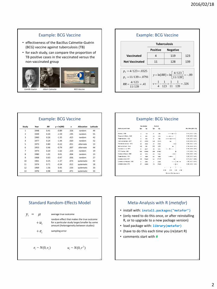
Example: BCG Vaccine
• effectiveness of the Bacillus Calmette-Guérin (BCG) vaccine against tuberculosis (TB)
• for each study, can compare the proportion of TB positive cases in the vaccinated versus the non-vaccinated group
Albert Calmette Camille Guérin BCG Vaccine 9
Example: BCG Vaccine
0791.139/11 Cp
41.139/11
123/4RR
0325.123/4 Tp
89.139/11
123/4ln]ln[
RRy
326.139
1
11
1
123
1
4
1v
Tuberculosis
Positive Negative
Vaccinated 4 119 123
Not Vaccinated 11 128 139
10
Example: BCG Vaccine
Study Year RR y = ln(RR) v Allocation Latitude
1 1948 0.41 -0.89 .326 random 44
2 1949 0.20 -1.59 .195 random 55
3 1960 0.26 -1.35 .415 random 42
4 1977 0.24 -1.44 .020 random 52
5 1973 0.80 -0.22 .051 alternate 13
6 1953 0.46 -0.79 .007 alternate 44
7 1973 0.20 -1.62 .223 random 19
8 1980 1.01 0.01 .004 random 13
9 1968 0.63 -0.47 .056 random 27
10 1961 0.25 -1.37 .073 systematic 42
11 1974 0.71 -0.34 .012 systematic 18
12 1969 1.56 0.45 .533 systematic 33
13 1976 0.98 -0.02 .071 systematic 33
11
Example: BCG Vaccine
12
Standard Random-Effects Model
i
i
i
e
u
y
average true outcome
random effect that makes the true outcome for a particular study larger/smaller by some amount (heterogeneity between studies)
sampling error
),0(~ 2Nui),0(~ ii vNe
13
Meta-Analysis with R (metafor)
• install with: install.packages("metafor")
• (only need to do this once, or after reinstalling R, or to upgrade to a new package version)
• load package with: library(metafor)
• (have to do this each time you (re)start R)
• comments start with #
2016/02/18
3
14
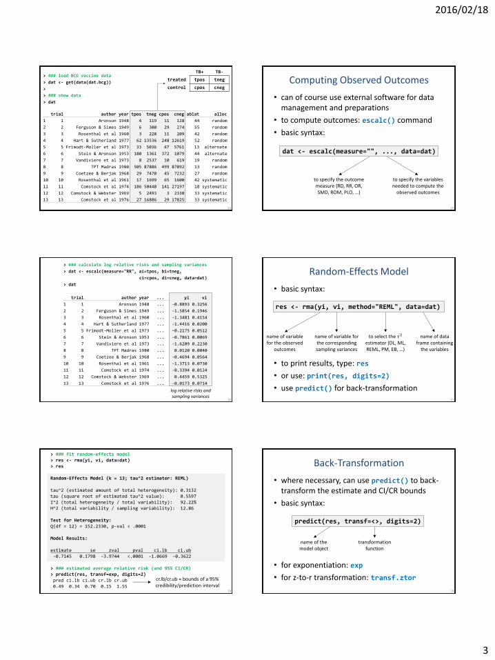
o
> ### load BCG vaccine data
> dat <- get(data(dat.bcg))
>
> ### show data
> dat
trial author year tpos tneg cpos cneg ablat alloc
1 1 Aronson 1948 4 119 11 128 44 random
2 2 Ferguson & Simes 1949 6 300 29 274 55 random
3 3 Rosenthal et al 1960 3 228 11 209 42 random
4 4 Hart & Sutherland 1977 62 13536 248 12619 52 random
5 5 Frimodt-Moller et al 1973 33 5036 47 5761 13 alternate
6 6 Stein & Aronson 1953 180 1361 372 1079 44 alternate
7 7 Vandiviere et al 1973 8 2537 10 619 19 random
8 8 TPT Madras 1980 505 87886 499 87892 13 random
9 9 Coetzee & Berjak 1968 29 7470 45 7232 27 random
10 10 Rosenthal et al 1961 17 1699 65 1600 42 systematic
11 11 Comstock et al 1974 186 50448 141 27197 18 systematic
12 12 Comstock & Webster 1969 5 2493 3 2338 33 systematic
13 13 Comstock et al 1976 27 16886 29 17825 33 systematic
TB+ TB-
treated tpos tneg
control cpos cneg
15
Computing Observed Outcomes
• can of course use external software for data management and preparations
• to compute outcomes: escalc() command
• basic syntax:
to specify the outcome measure (RD, RR, OR, SMD, ROM, PLO, …)
to specify the variables needed to compute the
observed outcomes
dat <- escalc(measure="", ..., data=dat)
16
> ### calculate log relative risks and sampling variances
> dat <- escalc(measure="RR", ai=tpos, bi=tneg,
ci=cpos, di=cneg, data=dat)
> dat
trial author year ... yi vi
1 1 Aronson 1948 ... -0.8893 0.3256
2 2 Ferguson & Simes 1949 ... -1.5854 0.1946
3 3 Rosenthal et al 1960 ... -1.3481 0.4154
4 4 Hart & Sutherland 1977 ... -1.4416 0.0200
5 5 Frimodt-Moller et al 1973 ... -0.2175 0.0512
6 6 Stein & Aronson 1953 ... -0.7861 0.0069
7 7 Vandiviere et al 1973 ... -1.6209 0.2230
8 8 TPT Madras 1980 ... 0.0120 0.0040
9 9 Coetzee & Berjak 1968 ... -0.4694 0.0564
10 10 Rosenthal et al 1961 ... -1.3713 0.0730
11 11 Comstock et al 1974 ... -0.3394 0.0124
12 12 Comstock & Webster 1969 ... 0.4459 0.5325
13 13 Comstock et al 1976 ... -0.0173 0.0714
log relative risks and sampling variances
17
Random-Effects Model
• basic syntax:
• to print results, type: res
• or use: print(res, digits=2)
• use predict() for back-transformation
to select the 𝜏2 estimator (DL, ML, REML, PM, EB, …)
res <- rma(yi, vi, method="REML", data=dat)
name of variable for the observed
outcomes
name of data frame containing
the variables
name of variable for the corresponding sampling variances
18
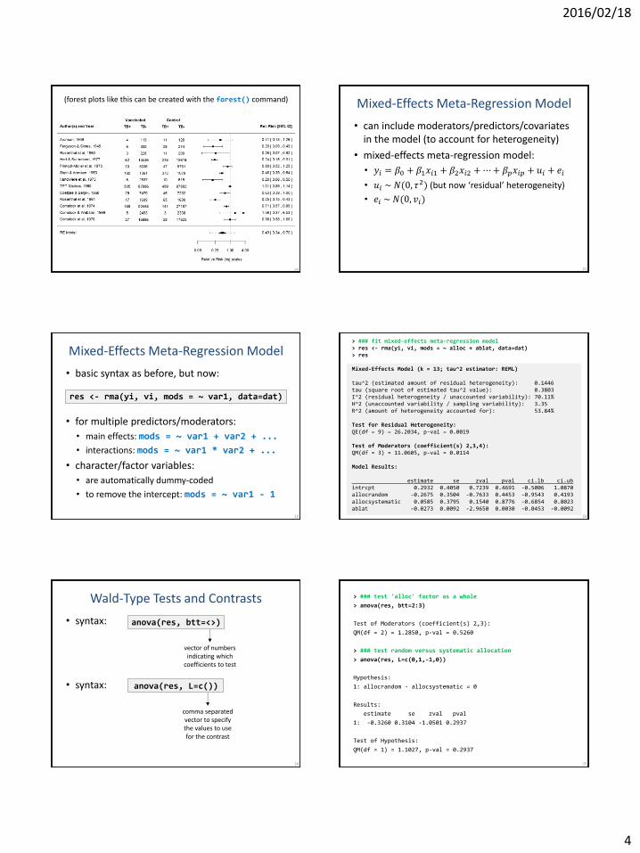
> ### fit random-effects model > res <- rma(yi, vi, data=dat) > res Random-Effects Model (k = 13; tau^2 estimator: REML) tau^2 (estimated amount of total heterogeneity): 0.3132 tau (square root of estimated tau^2 value): 0.5597 I^2 (total heterogeneity / total variability): 92.22% H^2 (total variability / sampling variability): 12.86 Test for Heterogeneity: Q(df = 12) = 152.2330, p-val < .0001 Model Results: estimate se zval pval ci.lb ci.ub -0.7145 0.1798 -3.9744 <.0001 -1.0669 -0.3622 > ### estimated average relative risk (and 95% CI/CR) > predict(res, transf=exp, digits=2) pred ci.lb ci.ub cr.lb cr.ub 0.49 0.34 0.70 0.15 1.55
cr.lb/cr.ub = bounds of a 95% credibility/prediction interval
19
Back-Transformation
• where necessary, can use predict() to back-transform the estimate and CI/CR bounds
• basic syntax:
• for exponentiation: exp
• for z-to-r transformation: transf.ztor
name of the model object
transformation function
predict(res, transf=<>, digits=2)
2016/02/18
4
20
(forest plots like this can be created with the forest() command)
21
Mixed-Effects Meta-Regression Model
• can include moderators/predictors/covariates in the model (to account for heterogeneity)
• mixed-effects meta-regression model:
• 𝑦𝑖 = 𝛽0 + 𝛽1𝑥𝑖1 + 𝛽2𝑥𝑖2 + ⋯ + 𝛽𝑝𝑥𝑖𝑝 + 𝑢𝑖 + 𝑒𝑖
• 𝑢𝑖 ~ 𝑁(0, 𝜏2) (but now ‘residual’ heterogeneity)
• 𝑒𝑖 ~ 𝑁(0, 𝑣𝑖)
22
Mixed-Effects Meta-Regression Model
• basic syntax as before, but now:
• for multiple predictors/moderators:
• main effects: mods = ~ var1 + var2 + ...
• interactions: mods = ~ var1 * var2 + ...
• character/factor variables:
• are automatically dummy-coded
• to remove the intercept: mods = ~ var1 - 1
res <- rma(yi, vi, mods = ~ var1, data=dat)
23
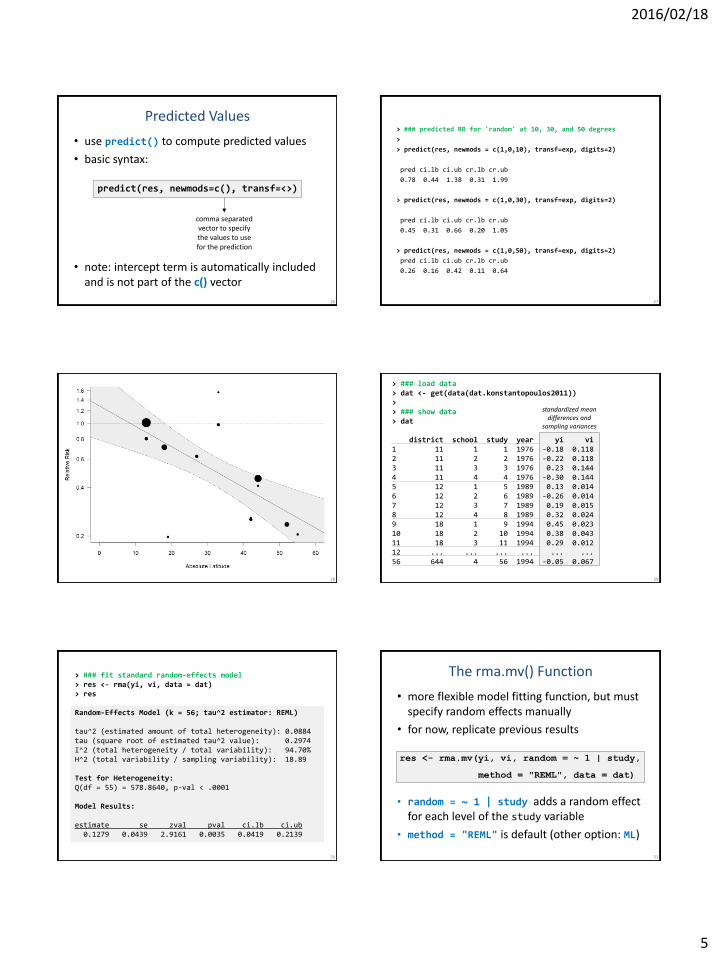
> ### fit mixed-effects meta-regression model > res <- rma(yi, vi, mods = ~ alloc + ablat, data=dat) > res Mixed-Effects Model (k = 13; tau^2 estimator: REML) tau^2 (estimated amount of residual heterogeneity): 0.1446 tau (square root of estimated tau^2 value): 0.3803 I^2 (residual heterogeneity / unaccounted variability): 70.11% H^2 (unaccounted variability / sampling variability): 3.35 R^2 (amount of heterogeneity accounted for): 53.84% Test for Residual Heterogeneity: QE(df = 9) = 26.2034, p-val = 0.0019 Test of Moderators (coefficient(s) 2,3,4): QM(df = 3) = 11.0605, p-val = 0.0114 Model Results: estimate se zval pval ci.lb ci.ub intrcpt 0.2932 0.4050 0.7239 0.4691 -0.5006 1.0870 allocrandom -0.2675 0.3504 -0.7633 0.4453 -0.9543 0.4193 allocsystematic 0.0585 0.3795 0.1540 0.8776 -0.6854 0.8023 ablat -0.0273 0.0092 -2.9650 0.0030 -0.0453 -0.0092
24
Wald-Type Tests and Contrasts
• syntax:
• syntax:
vector of numbers indicating which
coefficients to test
anova(res, btt=<>)
comma separated vector to specify the values to use for the contrast
anova(res, L=c())
25
> ### test 'alloc' factor as a whole
> anova(res, btt=2:3)
Test of Moderators (coefficient(s) 2,3):
QM(df = 2) = 1.2850, p-val = 0.5260
> ### test random versus systematic allocation
> anova(res, L=c(0,1,-1,0))
Hypothesis:
1: allocrandom - allocsystematic = 0
Results:
estimate se zval pval
1: -0.3260 0.3104 -1.0501 0.2937
Test of Hypothesis:
QM(df = 1) = 1.1027, p-val = 0.2937
2016/02/18
5
26
Predicted Values
• use predict() to compute predicted values
• basic syntax:
• note: intercept term is automatically included and is not part of the c() vector
comma separated vector to specify the values to use for the prediction
predict(res, newmods=c(), transf=<>)
27
> ### predicted RR for 'random' at 10, 30, and 50 degrees
>
> predict(res, newmods = c(1,0,10), transf=exp, digits=2)
pred ci.lb ci.ub cr.lb cr.ub
0.78 0.44 1.38 0.31 1.99
> predict(res, newmods = c(1,0,30), transf=exp, digits=2)
pred ci.lb ci.ub cr.lb cr.ub
0.45 0.31 0.66 0.20 1.05
> predict(res, newmods = c(1,0,50), transf=exp, digits=2)
pred ci.lb ci.ub cr.lb cr.ub
0.26 0.16 0.42 0.11 0.64
28 29
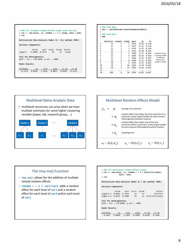
> ### load data > dat <- get(data(dat.konstantopoulos2011)) > > ### show data > dat district school study year yi vi 1 11 1 1 1976 -0.18 0.118 2 11 2 2 1976 -0.22 0.118 3 11 3 3 1976 0.23 0.144 4 11 4 4 1976 -0.30 0.144 5 12 1 5 1989 0.13 0.014 6 12 2 6 1989 -0.26 0.014 7 12 3 7 1989 0.19 0.015 8 12 4 8 1989 0.32 0.024 9 18 1 9 1994 0.45 0.023 10 18 2 10 1994 0.38 0.043 11 18 3 11 1994 0.29 0.012 12 ... ... ... ... ... ... 56 644 4 56 1994 -0.05 0.067
standardized mean differences and
sampling variances
30
> ### fit standard random-effects model > res <- rma(yi, vi, data = dat) > res Random-Effects Model (k = 56; tau^2 estimator: REML) tau^2 (estimated amount of total heterogeneity): 0.0884 tau (square root of estimated tau^2 value): 0.2974 I^2 (total heterogeneity / total variability): 94.70% H^2 (total variability / sampling variability): 18.89 Test for Heterogeneity: Q(df = 55) = 578.8640, p-val < .0001 Model Results: estimate se zval pval ci.lb ci.ub 0.1279 0.0439 2.9161 0.0035 0.0419 0.2139
31
The rma.mv() Function
• more flexible model fitting function, but must specify random effects manually
• for now, replicate previous results
• random = ~ 1 | study adds a random effect for each level of the study variable
• method = "REML" is default (other option: ML)
res <- rma.mv(yi, vi, random = ~ 1 | study,
method = "REML", data = dat)
2016/02/18
6
32
> ### fit standard random-effects model with rma.mv() > res <- rma.mv(yi, vi, random = ~ 1 | study, data = dat) > res Multivariate Meta-Analysis Model (k = 56; method: REML) Variance Components: estim sqrt nlvls fixed factor sigma^2 0.0884 0.2974 56 no study Test for Heterogeneity: Q(df = 55) = 578.8640, p-val < .0001 Model Results: estimate se zval pval ci.lb ci.ub 0.1279 0.0439 2.9161 0.0035 0.0419 0.2139
33
> ### load data > dat <- get(data(dat.konstantopoulos2011)) > > ### show data > dat district school study year yi vi 1 11 1 1 1976 -0.18 0.118 2 11 2 2 1976 -0.22 0.118 3 11 3 3 1976 0.23 0.144 4 11 4 4 1976 -0.30 0.144 5 12 1 5 1989 0.13 0.014 6 12 2 6 1989 -0.26 0.014 7 12 3 7 1989 0.19 0.015 8 12 4 8 1989 0.32 0.024 9 18 1 9 1994 0.45 0.023 10 18 2 10 1994 0.38 0.043 11 18 3 11 1994 0.29 0.012 12 ... ... ... ... ... ... 56 644 4 56 1994 -0.05 0.067
between 3 and 11 schools within
11 different districts (56
studies in total)
34
Multilevel Meta-Analytic Data
• multilevel structures can arise when we have multiple estimates for some higher clustering variable (paper, lab, research group, …)
. . . Cluster 1
𝑦11 𝑦12
Cluster 2
𝑦𝑘2 𝑦2
Cluster k
𝑦𝑘1 𝑦𝑘3 . . .
35
Multilevel Random-Effects Model
ij
ij
i
ij
e
u
w
y
average true outcome
random effect that makes the true outcomes for a particular cluster larger/smaller by some amount (heterogeneity between clusters)
random effect that makes one of the true outcomes within a particular cluster larger/smaller by some amount (heterogeneity within clusters)
sampling error
),0(~ 2
Bi Nw ),0(~ 2
Wij Nu ),0(~ ijij vNe
36
The rma.mv() Function
• rma.mv() allows for the addition of multiple nested random effects
• random = ~ 1 | var1/var2 adds a random effect for each level of var1 and a random effect for each level of var2 within each level of var1
37
> ### fit multilevel random-effects model > res <- rma.mv(yi, vi, random = ~ 1 | district/school, data = dat) > res Multivariate Meta-Analysis Model (k = 56; method: REML) Variance Components: estim sqrt nlvls fixed factor sigma^2.1 0.0651 0.2551 11 no district sigma^2.2 0.0327 0.1809 56 no district/school Test for Heterogeneity: Q(df = 55) = 578.8640, p-val < .0001 Model Results: estimate se zval pval ci.lb ci.ub 0.1847 0.0846 2.1845 0.0289 0.0190 0.3504
2016/02/18
7
38
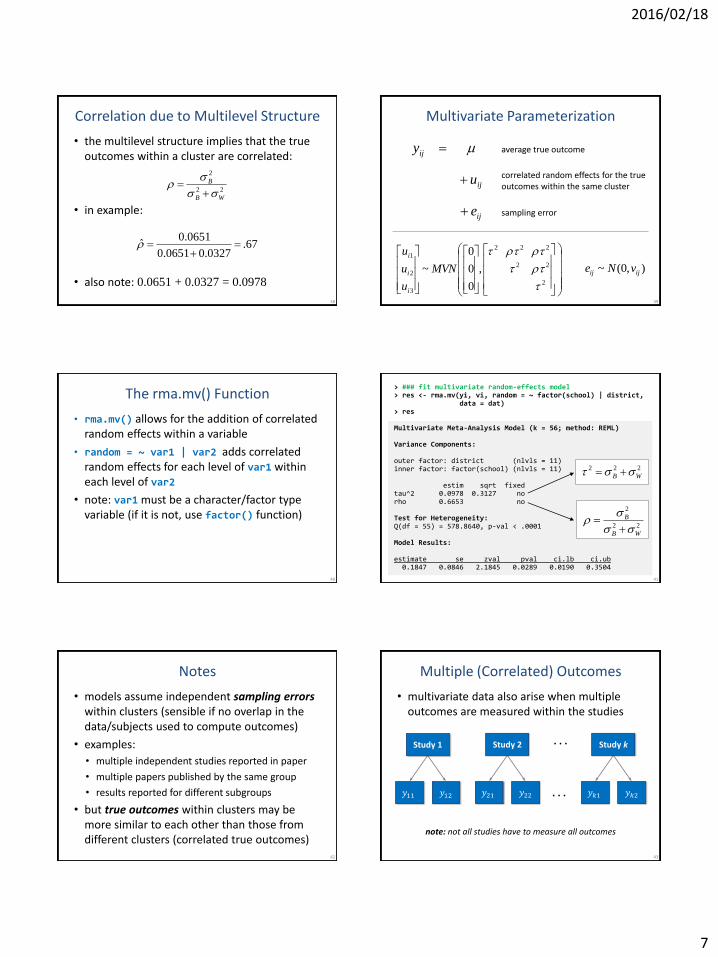
Correlation due to Multilevel Structure
• the multilevel structure implies that the true outcomes within a cluster are correlated:
• in example:
• also note: 0.0651 + 0.0327 = 0.0978
22
2
WB
B
67.0.03270.0651
0.0651ˆ
39
Multivariate Parameterization
ij
ij
ij
e
u
y
average true outcome
correlated random effects for the true outcomes within the same cluster
sampling error
2
22
222
3
2
1
,
0
0
0
~
MVN
u
u
u
i
i
i
),0(~ ijij vNe
40
The rma.mv() Function
• rma.mv() allows for the addition of correlated random effects within a variable
• random = ~ var1 | var2 adds correlated random effects for each level of var1 within each level of var2
• note: var1 must be a character/factor type variable (if it is not, use factor() function)
41
> ### fit multivariate random-effects model > res <- rma.mv(yi, vi, random = ~ factor(school) | district, data = dat) > res Multivariate Meta-Analysis Model (k = 56; method: REML) Variance Components: outer factor: district (nlvls = 11) inner factor: factor(school) (nlvls = 11) estim sqrt fixed tau^2 0.0978 0.3127 no rho 0.6653 no Test for Heterogeneity: Q(df = 55) = 578.8640, p-val < .0001 Model Results: estimate se zval pval ci.lb ci.ub 0.1847 0.0846 2.1845 0.0289 0.0190 0.3504
222
WB
22
2
WB
B
42
Notes
• models assume independent sampling errors within clusters (sensible if no overlap in the data/subjects used to compute outcomes)
• examples:
• multiple independent studies reported in paper
• multiple papers published by the same group
• results reported for different subgroups
• but true outcomes within clusters may be more similar to each other than those from different clusters (correlated true outcomes)
43
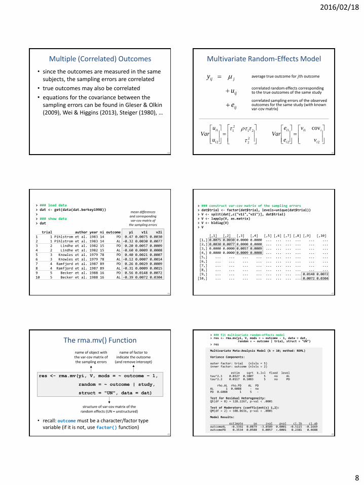
Multiple (Correlated) Outcomes
• multivariate data also arise when multiple outcomes are measured within the studies
. . . Study 1
𝑦11 𝑦12 . . .
Study 2
𝑦21 𝑦22
Study k
𝑦𝑘1 𝑦𝑘2
note: not all studies have to measure all outcomes
2016/02/18
8
44
Multiple (Correlated) Outcomes
• since the outcomes are measured in the same subjects, the sampling errors are correlated
• true outcomes may also be correlated
• equations for the covariance between the sampling errors can be found in Gleser & Olkin (2009), Wei & Higgins (2013), Steiger (1980), …
45
Multivariate Random-Effects Model
ij
ij
jij
e
u
y
average true outcome for 𝑗th outcome
correlated random effects corresponding to the true outcomes of the same study
correlated sampling errors of the observed outcomes for the same study (with known var-cov matrix)
2
2
21
2
1
2
1
i
i
u
uVar
2
1
2
1 cov
i
ii
i
i
v
v
e
eVar
46
> ### load data > dat <- get(data(dat.berkey1998)) > > ### show data > dat trial author year ni outcome yi v1i v2i 1 1 Pihlstrom et al. 1983 14 PD 0.47 0.0075 0.0030 2 1 Pihlstrom et al. 1983 14 AL -0.32 0.0030 0.0077 3 2 Lindhe et al. 1982 15 PD 0.20 0.0057 0.0009 4 2 Lindhe et al. 1982 15 AL -0.60 0.0009 0.0008 5 3 Knowles et al. 1979 78 PD 0.40 0.0021 0.0007 6 3 Knowles et al. 1979 78 AL -0.12 0.0007 0.0014 7 4 Ramfjord et al. 1987 89 PD 0.26 0.0029 0.0009 8 4 Ramfjord et al. 1987 89 AL -0.31 0.0009 0.0015 9 5 Becker et al. 1988 16 PD 0.56 0.0148 0.0072 10 5 Becker et al. 1988 16 AL -0.39 0.0072 0.0304
mean differences and corresponding var-cov matrix of
the sampling errors
47
> ### construct var-cov matrix of the sampling errors > dat$trial <- factor(dat$trial, levels=unique(dat$trial)) > V <- split(dat[,c("v1i","v2i")], dat$trial) > V <- lapply(V, as.matrix) > V <- bldiag(V) > V [,1] [,2] [,3] [,4] [,5] [,6] [,7] [,8] [,9] [,10] [1,] 0.0075 0.0030 0.0000 0.0000 ... ... ... ... ... ... [2,] 0.0030 0.0077 0.0000 0.0000 ... ... ... ... ... ... [3,] 0.0000 0.0000 0.0057 0.0009 ... ... ... ... ... ... [4,] 0.0000 0.0000 0.0009 0.0008 ... ... ... ... ... ... [5,] ... ... ... ... ... ... ... ... ... ... [6,] ... ... ... ... ... ... ... ... ... ... [7,] ... ... ... ... ... ... ... ... ... ... [8,] ... ... ... ... ... ... ... ... ... ... [9,] ... ... ... ... ... ... ... ... 0.0148 0.0072 [10,] ... ... ... ... ... ... ... ... 0.0072 0.0304
48
The rma.mv() Function
• recall: outcome must be a character/factor type variable (if it is not, use factor() function)
structure of var-cov matrix of the random effects (UN = unstructured)
name of object with the var-cov matrix of the sampling errors
name of factor to indicate the outcome
(and remove intercept)
res <- rma.mv(yi, V, mods = ~ outcome – 1,
random = ~ outcome | study,
struct = "UN", data = dat)
49
> ### fit multivariate random-effects model > res <- rma.mv(yi, V, mods = ~ outcome - 1, data = dat, random = ~ outcome | trial, struct = "UN") > res Multivariate Meta-Analysis Model (k = 10; method: REML) Variance Components: outer factor: trial (nlvls = 5) inner factor: outcome (nlvls = 2) estim sqrt k.lvl fixed level tau^2.1 0.0327 0.1807 5 no AL tau^2.2 0.0117 0.1083 5 no PD rho.AL rho.PD AL PD AL 1 0.6088 - no PD 0.6088 1 5 - Test for Residual Heterogeneity: QE(df = 8) = 128.2267, p-val < .0001 Test of Moderators (coefficient(s) 1,2): QM(df = 2) = 108.8616, p-val < .0001 Model Results: estimate se zval pval ci.lb ci.ub outcomeAL -0.3392 0.0879 -3.8589 0.0001 -0.5115 -0.1669 outcomePD 0.3534 0.0588 6.0057 <.0001 0.2381 0.4688
2016/02/18
9
50
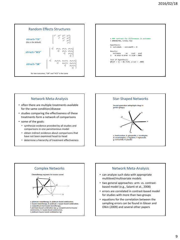
Random Effects Structures
𝜏2 𝜌𝜏2 𝜌𝜏2 𝜌𝜏2
𝜌𝜏2 𝜏2 𝜌𝜏2 𝜌𝜏2
𝜌𝜏2 𝜌𝜏2 𝜏2 𝜌𝜏2
𝜌𝜏 𝜌𝜏 𝜌𝜏 𝜏2
𝜏12 𝜌𝜏1𝜏2 𝜌𝜏1𝜏3 𝜌𝜏1𝜏4
𝜌𝜏1𝜏2 𝜏22 𝜌𝜏2𝜏3 𝜌𝜏2𝜏4
𝜌𝜏1𝜏3 𝜌𝜏2𝜏3 𝜏32 𝜌𝜏3𝜏4
𝜌𝜏1𝜏4 𝜌𝜏2𝜏4 𝜌𝜏3𝜏4 𝜏42
𝜏12 𝜌12𝜏1𝜏2 𝜌13𝜏1𝜏3 𝜌14𝜏1𝜏4
𝜌12𝜏1𝜏2 𝜏22 𝜌23𝜏2𝜏3 𝜌24𝜏2𝜏4
𝜌13𝜏1𝜏3 𝜌23𝜏2𝜏3 𝜏32 𝜌34𝜏4𝜏4
𝜌14𝜏1𝜏4 𝜌24𝜏2𝜏4 𝜌34𝜏3𝜏4 𝜏42
struct="CS"
struct="HCS"
struct="UN"
(this is the default)
for two outcomes, "UN" and "HCS" is the same 51
> ### contrast for differences in outcomes > anova(res, L=c(1,-1)) Hypothesis: 1: outcomeAL - outcomePD = 0 Results: estimate se zval pval 1: -0.6926 0.0744 -9.3120 <.0001 Test of Hypothesis: QM(df = 1) = 86.7139, p-val < .0001
52
Network Meta-Analysis
• often there are multiple treatments available for the same condition/disease
• studies comparing the effectiveness of these treatments form a network of comparisons
• some of the goals:
• synthesize evidence provided by all studies and comparisons in one parsimonious model
• obtain indirect evidence about comparisons that have not been examined head-to-head
• determine a hierarchy of treatment effectiveness
53
Star-Shaped Networks
54
Complex Networks
55
Network Meta-Analysis
• can analyze such data with appropriate multilevel/multivariate models
• two general approaches: arm- vs. contrast-based model (e.g., Salanti et al., 2008)
• errors are correlated in contrast-based model for studies with more than two groups
• equations for the correlation between the sampling errors can be found in Gleser and Olkin (2009) and several other papers
2016/02/18
10
56
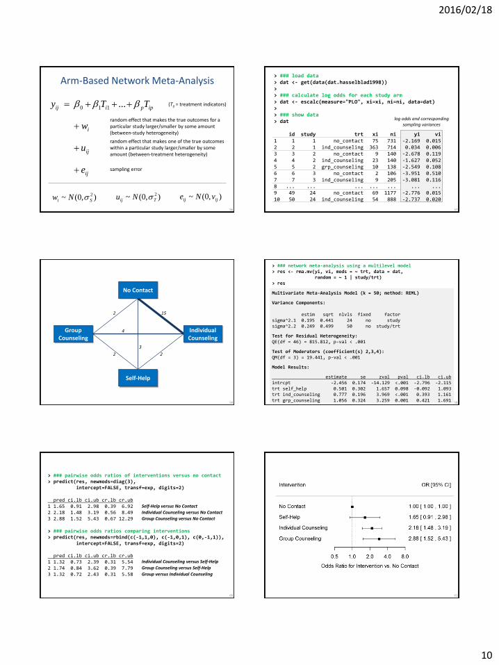
Arm-Based Network Meta-Analysis
ij
ij
i
ippiij
e
u
w
TTy
...110
),0(~ 2
Si Nw ),0(~ 2
Tij Nu ),0(~ ijij vNe
random effect that makes the true outcomes for a particular study larger/smaller by some amount (between-study heterogeneity)
random effect that makes one of the true outcomes within a particular study larger/smaller by some amount (between-treatment heterogeneity)
sampling error
(Tij = treatment indicators)
57
> ### load data > dat <- get(data(dat.hasselblad1998)) > > ### calculate log odds for each study arm > dat <- escalc(measure="PLO", xi=xi, ni=ni, data=dat) > > ### show data > dat id study trt xi ni yi vi 1 1 1 no_contact 75 731 -2.169 0.015 2 2 1 ind_counseling 363 714 0.034 0.006 3 3 2 no_contact 9 140 -2.678 0.119 4 4 2 ind_counseling 23 140 -1.627 0.052 5 5 2 grp_counseling 10 138 -2.549 0.108 6 6 3 no_contact 2 106 -3.951 0.510 7 7 3 ind_counseling 9 205 -3.081 0.116 8 ... ... ... ... ... ... ... 9 49 24 no_contact 69 1177 -2.776 0.015 10 50 24 ind_counseling 54 888 -2.737 0.020
log odds and corresponding sampling variances
58
Individual Counseling
Group Counseling
Self-Help
No Contact
15
4
2
3
2 2
59
> ### network meta-analysis using a multilevel model > res <- rma.mv(yi, vi, mods = ~ trt, data = dat, random = ~ 1 | study/trt) > res
Multivariate Meta-Analysis Model (k = 50; method: REML)
Variance Components: estim sqrt nlvls fixed factor sigma^2.1 0.195 0.441 24 no study sigma^2.2 0.249 0.499 50 no study/trt
Test for Residual Heterogeneity: QE(df = 46) = 815.812, p-val < .001
Test of Moderators (coefficient(s) 2,3,4): QM(df = 3) = 19.441, p-val < .001
Model Results:
estimate se zval pval ci.lb ci.ub intrcpt -2.456 0.174 -14.129 <.001 -2.796 -2.115 trt self_help 0.501 0.302 1.657 0.098 -0.092 1.093 trt ind_counseling 0.777 0.196 3.969 <.001 0.393 1.161 trt grp_counseling 1.056 0.324 3.259 0.001 0.421 1.691
60
> ### pairwise odds ratios of interventions versus no contact > predict(res, newmods=diag(3), intercept=FALSE, transf=exp, digits=2) pred ci.lb ci.ub cr.lb cr.ub 1 1.65 0.91 2.98 0.39 6.92 2 2.18 1.48 3.19 0.56 8.49 3 2.88 1.52 5.43 0.67 12.29 > ### pairwise odds ratios comparing interventions > predict(res, newmods=rbind(c(-1,1,0), c(-1,0,1), c(0,-1,1)), intercept=FALSE, transf=exp, digits=2) pred ci.lb ci.ub cr.lb cr.ub 1 1.32 0.73 2.39 0.31 5.54 2 1.74 0.84 3.62 0.39 7.79 3 1.32 0.72 2.43 0.31 5.58
Self-Help versus No Contact
Individual Counseling versus No Contact
Group Counseling versus No Contact
Individual Counseling versus Self-Help
Group Counseling versus Self-Help
Group versus Individual Counseling
61
2016/02/18
11
62
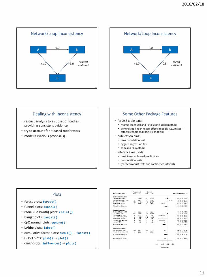
Network/Loop Inconsistency
B
C
A
+1.0 +1.0
0.0
(indirect evidence)
63
Network/Loop Inconsistency
B
C
A
+1.0 -0.5
0.0
(direct evidence)
64
Dealing with Inconsistency
• restrict analysis to a subset of studies providing consistent evidence
• try to account for it based moderators
• model it (various proposals)
65
Some Other Package Features
• for 2x2 table data: • Mantel-Haenszel and Peto's (one-step) method
• generalized linear mixed-effects models (i.e., mixed-effects (conditional) logistic models)
• publication bias: • rank correlation test
• Egger's regression test
• trim and fill method
• inference methods: • best linear unbiased predictions
• permutation tests
• (cluster) robust tests and confidence intervals
66
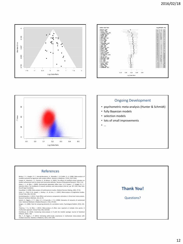
Plots
• forest plots: forest()
• funnel plots: funnel()
• radial (Galbraith) plots: radial()
• Baujat plots: baujat()
• Q-Q normal plots: qqnorm()
• L’Abbé plots: labbe()
• cumulative forest plots: cumul() → forest()
• GOSH plots: gosh() → plot()
• diagnostics: influence() → plot()
67
2016/02/18
12
68 69
70 71
Ongoing Development
• psychometric meta-analysis (Hunter & Schmidt)
• fully Bayesian models
• selection models
• lots of small improvements
• …
72
References Berkey, C. S., Hoaglin, D. C., Antczak-Bouckoms, A., Mosteller, F., & Colditz, G. A. (1998). Meta-analysis of multiple outcomes by regression with random effects. Statistics in Medicine, 17(22), 2537-2550.
Cooper, H., Valentine, J. C., Charlton, K., & Melson, A. (2003). The effects of modified school calendars on student achievement and on school and community attitudes. Review of Educational Research, 73(1), 1-52.
Gleser, L. J., & Olkin, I. (2009). Stochastically dependent effect sizes. In H. Cooper, L. V. Hedges, & J. C. Valentine (Eds.), The handbook of research synthesis and meta-analysis (2nd ed., pp. 357–376). New York: Russell Sage Foundation.
Hasselblad, V. (1998). Meta-analysis of multitreatment studies. Medical Decision Making, 18(1), 37-43.
Ishak, K. J., Platt, R. W., Joseph, L., Hanley, J. A., & Caro, J. J. (2007). Meta-analysis of longitudinal studies. Clinical Trials, 4(5), 525-539.
Konstantopoulos, S. (2011). Fixed effects and variance components estimation in three-level meta-analysis. Research Synthesis Methods, 2(1), 61-76.
Salanti, G., Higgins, J. P. T., Ades, A. E., & Ioannidis, J. P. A. (2008). Evaluation of networks of randomized trials. Statistical Methods in Medical Research, 17(3), 279-301.
Steiger, J. H. (1980). Tests for comparing elements of a correlation matrix. Psychological Bulletin, 87(2), 245-251.
Trikalinos, T. A., & Olkin, I. (2012). Meta-analysis of effect sizes reported at multiple time points: A multivariate approach. Clinical Trials, 9(5), 610-620.
Viechtbauer, W. (2010). Conducting meta-analyses in R with the metafor package. Journal of Statistical Software, 36(3), 1-48.
Wei, Y., & Higgins, J. P. (2013). Estimating within-study covariances in multivariate meta-analysis with multiple outcomes. Statistics in Medicine, 32(7), 1191-1205.
73
Thank You!
Questions?