Embed Size (px)
Citation preview

Research report 2013:06
Meta Modeling of Transmission Error for Spur, Helical and Planetary Gears for Wind Turbine Application M U H A M M A D I R F A N Department of Applied Mechanics C H A L M E R S U N I V E R S I T Y O F T E C H N O L O G Y Göteborg, Sweden 2013


Research report 2006:08
Meta Modeling of Transmission Error for Spur, Helical and Planetary Gears
for Wind Turbine Application
by
M U H A M M A D I R F A N
Department of Applied Mechanics CHALMERS UNIVERSITY OF TECHNOLOGY
Göteborg, Sweden, 2013

Meta Modeling of Transmission Error for Spur, Helical and Planetary Gears for Wind Turbine Application M U H A M M A D I R F A N © M U H A M M A D I R F A N , 2013 Research report 2013:06 ISSN 1652-8549 Department of Applied Mechanics Chalmers University of Technology SE-412 96 Göteborg Sweden Telephone +46 (0)31 772 1000

CHALMERS, Applied Mechanics, Research Report 2013:06 1
Abstract: Detailed analysis of drive train dynamics requires accounting for the transmission error that arises in gears. However, the direct computation of the transmission error requires a 3-dimensional contact analysis with correct gear geometry, which is impractically computationally intense. Therefore, a simplified representation of the transmission error is desired, a so-called meta-model, is developed. The model is based on response surface method, and the coefficients of the angle-dependent transmission error are dependent on shaft eccentricity (parallel misalignment), shaft bending (angular misalignment), torque and speed. Parallel spur gear, helical gear and planetary gear are studied, with parameters for wind turbine applications is considered and Abaqus 6.12-1 is used for the development of the meta-models. Upon evaluating the results, it is concluded that meta-modeling technique can be an efficient way of predicting the transmission error.
Keywords: Transmission error, Wind turbine, Meta-models, Spur gear, Helical gear, Planetary gear, Regression analysis.

CHALMERS, Applied Mechanics, Research Report 2013:06 2
Preface This work is carried out at the Division of Dynamics the Department of Applied Mechanics, Chalmers University of Technology, Gothenburg, Sweden, under the supervision of Professor Viktor Berbyuk and Lecturer Håkan Johansson. The work is part of the ongoing research into wind turbine drive train system dynamics supported by the Swedish Wind Power Technology Centre (SWPTC) [http://www.chalmers.se/ee/swptc-en].
The work is also reported as final thesis for M.Sc. degree in Mechanical Engineering with Emphasis on Structural Engineering at Blekinge University, Sweden. Formal examiner and subervisor from Blekinge was Ansel Berghuvud, Senior Lecturer at the Department of Mechanical Engineering, Karlskrona, Sweden.

CHALMERS, Applied Mechanics, Research Report 2013:06 3
Acknowledgement First and foremost, I would like to thank the Almighty ALLAH who blessed me the ability to complete this work. I would also like to thank my parents and other family members to provide me the support and love.
This work is carried out at the Division of Dynamics the Department of Applied Mechanics, Chalmers University of Technology, Gothenburg, Sweden, under the supervision of Professor Viktor Berbyuk and Lecturer Håkan Johansson. The work is part of the ongoing research into wind turbine drive train system dynamics supported by the Swedish Wind Power Technology Centre (SWPTC) [http://www.chalmers.se/ee/swptc-en]. The work is also supervised by Ansel Berghuvud, Senior Lecturer at the Department of Mechanical Engineering, Karlskrona, Sweden.
It is with immense gratitude that the work would not have been possible without the valuable ideas and comments of Håkan Johansson throughout the work period.
I also wish my sincere thanks to Ph.D. students Gaël Le Gigan, Shahab Teimourimanesh, and Xin Li at the Department of Applied Mechanics, Chalmers University of Technology, Gothenburg, Sweden, for extending the help.
Muhammad Irfan

CHALMERS, Applied Mechanics, Research Report 2013:06 4
Contents
1 Notations ......................................................................................................................................... 6
2 Introduction .................................................................................................................................... 8
3 Gear Modeling in Abaqus.............................................................................................................. 11
3.1 Gear Geometry and Part Module ........................................................................................................ 11 3.2 Material Module ................................................................................................................................. 12 3.3 Assembly Module ............................................................................................................................... 12 3.4 Steps Module ...................................................................................................................................... 12 3.5 Interaction Module ............................................................................................................................. 13 3.6 Load Module ...................................................................................................................................... 13 3.7 Boundary Module ............................................................................................................................... 13 3.8 Mesh Module ...................................................................................................................................... 13
4 Meta-Modeling .............................................................................................................................. 16
4.1 Regression Analysis ........................................................................................................................... 16 4.1.1 Random Discrete Variables ......................................................................................................... 16
4.1.2 The Analysis of Variance ............................................................................................................ 16
5 Results ........................................................................................................................................... 18
5.1 Spur Gear ............................................................................................................................................ 18 5.1.1 Radial Misalignment:S1 .............................................................................................................. 18
5.1.2. Angular Misalignment:S2 .......................................................................................................... 23
5.1.3. Radial and Angular Misalignment .............................................................................................. 26
5.1.4. Transmission error for torque:S3 ................................................................................................ 28
5.1.5. Transmission error for radial, angular, and torque:S4 ................................................................ 31
5.1.6. Transmission error for pressure angle:S5 ................................................................................... 32
5.1.7. Transmission error for gear ratio:S6 ........................................................................................... 34
5.1.8. Transmission error for addendum:S7 ......................................................................................... 36
5.2 Helical Gear ........................................................................................................................................ 38 5.2.1 Radial Misalignment:H1 ............................................................................................................. 38
5.2.2. Angular Misalignment:H2 .......................................................................................................... 39
5.2.3. Radial and Angular Misalignment .............................................................................................. 41
5.2.6. Transmission error for torque:H3 ............................................................................................... 42
5.2.5. Transmission error for radial, angular misalignments and torque:H4 ............................. 43
5.2.6. Transmission error for pressure angle:H5 .................................................................................. 44
5.2.7. Transmission error for gear ratio:H6 .......................................................................................... 45
5.2.8. Transmission error for addendum:H7 ........................................................................................ 46
5.2.9. Transmission error for helix angle:H8 ....................................................................................... 47

CHALMERS, Applied Mechanics, Research Report 2013:06 5
5.3 Planetary Gear .................................................................................................................................... 49 5.3.1. Radial and Angular Misalignment .............................................................................................. 49
5.3.2. Transmission error for radial, angular misalignments and Torque:P4 ............................ 51
5.3.3. Transmission error for radial, angular misalignments, torque, pressure angle, gear ratio, and addendum of planetary gears. ................................................................................................................ 51
5.3.4. Comparison of TE from meta-models and simulation ............................................................... 52
6 Evaluation ..................................................................................................................................... 54
6.1. Spur gear............................................................................................................................................ 54 6.2 Helical gear......................................................................................................................................... 57 6.3. Planetary gear .................................................................................................................................... 58
7 Conclusion ..................................................................................................................................... 59
8 Future work .................................................................................................................................. 60
References ......................................................................................................................................... 61
Appendices ........................................................................................................................................ 64
A. Matlab Coding for TE .......................................................................................................................... 64 B. Matlab Coding to Plot TE lines and Mean values ................................................................................ 65 C. Matlab Coding for Meta-model and Polynomial Fit of Coefficients .................................................... 66 D. Matlab Coding for Radial and Angular Misalignments Meta-models ................................................. 68 E. Meshing Technique ............................................................................................................................... 69

CHALMERS, Applied Mechanics, Research Report 2013:06 6
1 Notations
mm millimeter
MW Megawatt
𝑦 Dependent output variable
𝑥 Independent input variable
𝛽𝑜 Coefficient of model
𝜀 Random error
𝑏 Estimated coefficient
𝑅 Residual
𝑌 Out variable in matrix form
𝑋 Input variable in matrix form
𝐸 Estimated value
𝑉𝑎𝑟 Variance
𝐼𝑁 Identity matrix
𝜎2 Standard deviation
𝑌� Estimated output variable
𝑥𝑝′ Estimated input variable
𝑠2 Estimated standard deviation
𝑦� Average value
𝐹 Statistic estimation checking
𝐻𝑜 Null hypothesis
𝐻𝛼 Alternative hypothesis
𝑅2 Coefficient of determination
𝑅𝐴2 Adjusted statistic estimation
𝑡 Statistic estimation checking
C3D8R 8-node linear brick element
Indices
𝑝 Number of variables
𝑁 Number of observations
𝛼 Level of statistic estimation
A Adjusted statistic

CHALMERS, Applied Mechanics, Research Report 2013:06 7
Abbreviations
CAD Computer-aided design
IGES Initial graphics exchange specification
rpm Revolutions per minute
𝑆𝑆𝐸 Sum of squares of errors
TE Transmission error

CHALMERS, Applied Mechanics, Research Report 2013:06 8
2 Introduction
Since the occurrence of an oil crisis in the mid-seventies, energy policies have been diverted towards renewable energy resources. Since then wind turbine technology has received increasing attention as a renewable energy resource to produce electricity without emission of greenhouse gases during operation. The production capacity to generate electricity is growing day by day, according to the annual report of American Wind Energy Association the total U.S. utility-scale wind power capacity would be 60,007 MW after the completion of 43 MW till 4th quarter of 2012 [1]. The cost efficiency of wind turbine may increase with longer service life of gear boxes. To design gear boxes with longer service life engineers have different challenges. Better models for the drive train dynamics are demanded, particularly with respect to transmission error arising in indirect drive systems. Since turbine certification requires thousands of different analyses, these models should be efficient to evaluate. The drive train system is a crucial part to wind turbine as it transmits mechanical power from rotor hub to generator. Torque and rotational speed of the drive train system determine the designing power capacity of wind turbine. A common indirect drive train design consists of a multiple stage gearbox, coupling, break and generator. For current utility-scale wind turbine, mechanical power is transmitted from 12-30 rpm of turbines rotor to 1200-1800 rpm of generators rotor via two or more than stages of planetary gears [2].
Failure of the gearbox in drive train system has a negative effect on wind turbine income. It is the maintenance requirement to replace gearboxes every 7-11 years in a life time of 20 years [3] and gear boxes cost accounts for approximately 10 percent of construction and installation [4]. Sudden increase of wind speed, wind gusts, can be a cause to sudden peaks or transients in the loads affecting gearbox, particularly large bending moments. This can be one of the reasons for premature gearbox failures.
To avoid unexpected gear box failure it is important to understand the effect of different parameters in gear contact analysis. With particular geometry parameters of gears on different issues have been conducted: in [5] for pin stiffness and misalignment, in [6] , [7] and [5] dynamic analysis for tooth wedging and bearing clearance nonlinearities, transient regime, and eccentricities respectively. Sankar and Nataraj studied transmission error [8]. Robert and Parker examined how gear efficiency could be improved [9]. Finite element and analytical models techniques together were used in [10]. Similarly particular gear parameters to generate 3D gear were chosen for the work of [11] [12] [13] [14]. In this project the effect of different gear parameters will be analyzed on transmission error. Raul Tharmakulasingam examined effects of tooth profile modifications on gear pair [15]. X. Gu presented influence of eccentricity on planetary gear dynamics [5] [16]. Ramakrishnan observed effect of varies misalignment on planetary gears with time. In this thesis work eccentricity (radial misalignment) and shaft bending (angular misalignment) are also examined in addition to gear parameters. This analysis will be done by meta-modeling through regression analysis because dynamic simulation of gears contact can be easily evaluated through this meta-modeling.
“The deviation in position of the driven gear (for any given position of the driving gear), relative to the position that the driven gear would occupy if both gears were geometrically perfect and un-deformed [17].”
CHALMERS, Applied Mechanics, Research Report 2013:06 9
In appendix A, Matlab coding to calculate transmission error is given. Eccentricity, shaft bending, and vibrations are important factors for gear contact analysis. Wind gusts may cause uneven loading of the rotor’s torque which indirectly generates eccentricity of gear’s teeth. Tooth wears out unevenly due to this eccentricity and this additional wear causes more eccentricity and so on. Furthermore, machine chassis movement introduces eccentricity which can affect the performance of high speed rear gearing portion of gear boxes. In addition, shaft bending is another factor to be considered for the gearbox reliability. Shaft bending increases edge load in gear contact. That ultimately results in high contact stresses and shortens the gear life. Even a small variation of the force causes vibrations which can lead to mechanical noises or tonal noises. These noises can create a serious issue for residents in case of onshore wind turbines. So in Europe and North America some standards are fixed and if the operating wind turbine does not meet the standards, they can face heavy penalties. In the meshing of gear teeth, even a slightly varying contact force produces vibrations that accounts for mechanical noise. This issue is more severe for the high capacity wind turbines. Along with eccentricity and shaft bending, quality of gear is also a major factor to deal with the transmission error of gearboxes. That quality of gear which relates to the gear parameters including tooth width, tooth thickness, tooth profile, pitch of the gear, etc.
For longer life time service of drive train system, reliability and safeguards are more demanding for gearboxes because gearboxes of modern electrical utility in wind turbines are also the critical part of drive train system at Megawatt (MW) level of rated power [18]. In this project through one of the statistical approach, a regression analysis, transmission error will be analyzed at different input parameters of meshing gear settings.
For long time reliability, time domain simulations are required [19]. Rune Pedersen showed advantages and drawbacks of applying periodic time-variant modal analysis to spur gear dynamics [14]. Vijaya Kumar worked on complex non-linear dynamic behavior of planetary spur gears [10]. The main reason for meta-models is that computationally 3D full simulation of precise gears is too complex. A polynomial equation of meta-modeling will be established through regression analysis which is a statistical analysis. This polynomial will be recomputed on the behalf of changing input gear variables. Regression analysis optimizes the relationships between several independent input variables and one or more output response variables. In this project, a meta-model shall be determined for three different cases of gears, first for parallel spur gears, second for parallel helical gears, and third for planetary gears. Meta-models will provide behavior of transmission error at different input variables.
3D finite element simulation of gear contact analysis runs in Abaqus software. Before some researchers have already done different kind of gear analysis on Abaqus. Karimpour also used Abaqus for kinematics analysis of polymer gear tooth [20]. Raul [15] and Mao [21] utilized Abaqus for transmission error. For the work of [22] and [23] Abaqus was used for parking pawl mechanism and torsional stiffness of spur gears respectively. Gear simulation was also done in [24] [25] [26]. Results from Abaqus model are utilized for setting parameters in the meta-model. Autodesk inventor is used for the geometry of gears where only those input variables which are related to gear quality are introduced.

CHALMERS, Applied Mechanics, Research Report 2013:06 10
Figure 2.1. Introduction of dynamic variables to gear contact.
Figure 2.1. shows that how the dynamic variables (radial misalignment, angular misalignment and torque) will be introduced to gear contact analysis. Meta-model will determine transmission error at different values of the dynamic variables.

CHALMERS, Applied Mechanics, Research Report 2013:06 11
3 Gear Modeling in Abaqus
Abaqus is a general-purpose finite element base software for dynamic and quasi-static 2D and 3D simulations. To simulate gears rotation through abaqus is accomplished by different modules including part, material, assembly, steps, interaction, mesh, load, and boundary.
3.1 Gear Geometry and Part Module
3D geometrical model of gears can be developed by different available CAD softwares. Gears tooth profile can be formed automatically by these CAD sofwares or user can construct profile line by line. The CAD software ‘Autodesk Inventor Professional 2013’ is adopted in this thesis work. Standard (mm).iam assembly file is used for gear design geometry. In Design module automated gear component generator is available. This procedure is followed because this is one of the easy ways to generate 3D gear model just only on behalf of few parameters. In the chosen CAD software user can choose some parameters to create gear geometry. These optional parameters are desired gear ratio, module, centre distance, number of teeth, face width, pressure angle, helix angle, and total unit correction. User can also change unit tooth size by changing the value of addendum, clearance, and root fillet. For the case of meta-modeling of misalignment, shaft bending, and different applied torque, parametric values of Table 2.1. are chosen.
Parameter Assigned Value Desired gear ratio 2 Module 3mm Centre distance 90mm Number of teeth Pinion 20
Gear 40 Face Width 23mm Pressure angle 20o
Normal Backlash 0.513037mm Addendum 0.1 mm Clearance 0.25mm Root fillet 0.3mm
Table 2.2. Gear Parameters.
In table 2.3. the considered values for spur gears and helical gears are listed. For the geometry of planetary gears the same procedure will be followed. By selecting design guide options from the same module, user can define which kind of parameter is going to be design on the basis of other provided parametric values. Total unit correction is also selected. These all selected parameters are few parameters to form 3D model of a gear but Autodesk Inventor uses different standard measurement methods to form complete 3D model of a gear. For all gear models ISO 6336:1996 will be used as a strength calculation method.
Before importing the 3D models of gears to Abaqus, the models are saved in IGES files format through Autodesk Inventor. In part module of Abaqus, the models are imported. Imported geometries may not have accurate teeth profile but it is neglected. The 3D models can also be
CHALMERS, Applied Mechanics, Research Report 2013:06 12
created through Abaqus but for the work almost more than 40 models are required that’s why Autodesk Inventor Professional 2013-English is used.
3.2 Material Module
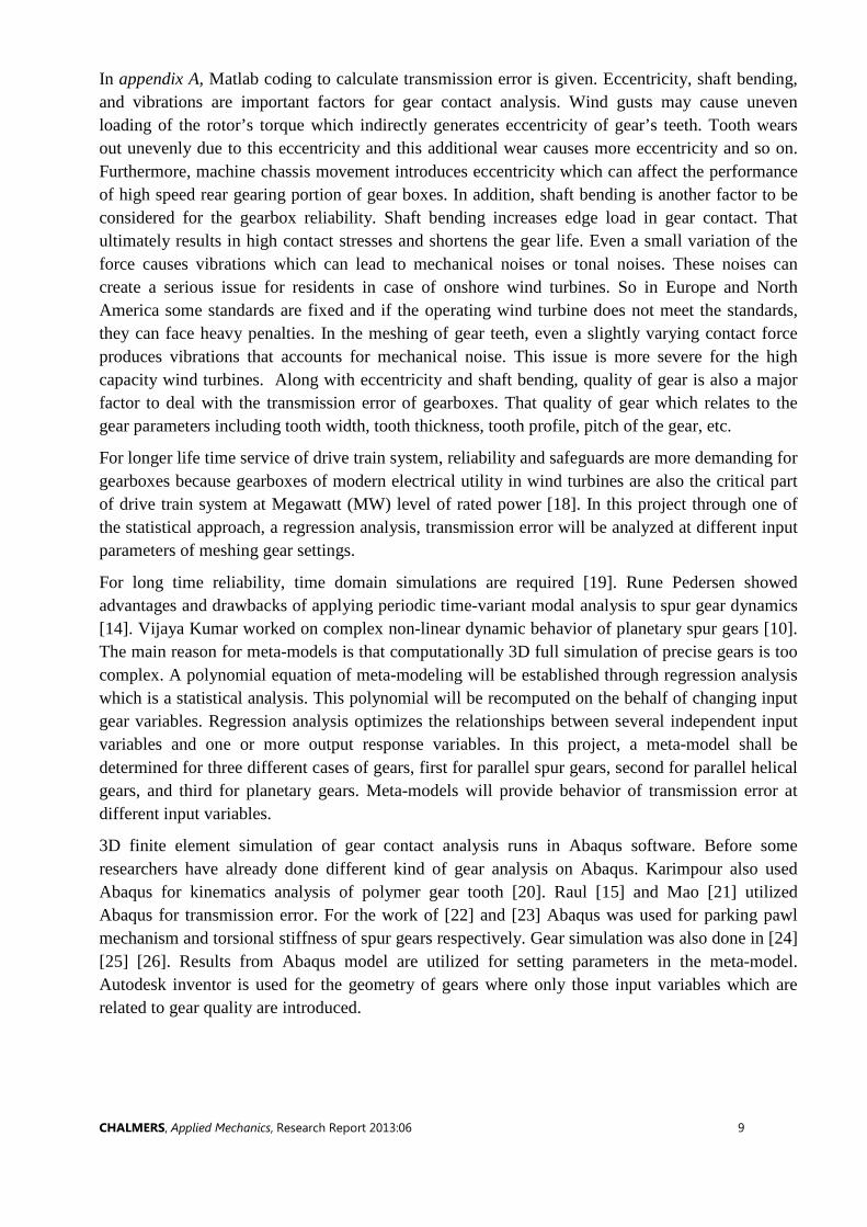
The next step is to define material properties of the 3D models in material module. As in this project focus is only on wind turbine application, so material properties selected in this project, should also reveal wind turbine application. A wide range of material properties are given for the purpose but following properties are chosen without further motivation.
Property Assigned Value Density 0.00803 g/mm3
Young’s Modulus 21000 N/mm2 Poison ratio 0.3 Mass damping 𝛼𝑅 [15]� 0.03 Stiffness damping 𝛽𝑅 [15]� 3E-6
Table 2.4. Material Properties.
3.3 Assembly Module
In this module gears are imported through instances selection and brought into the teeth contact position. Misalignment and shaft bending will be introduced through assembly module. To import mesh part, the gears treated as independent instances.
Figure 3.1. Assembly of gears.
3.4 Steps Module
Different kind of analysis can be defined in Abaqus like static general, dynamic implicit, dynamic explicit, heat transfer, mass diffusion etc. Linear and non-linear analysis can be performed through general analysis and linear analysis can also be performed by linear perturbation analysis. Static general is used for the gear analysis. Because non-linearity due to contact is expected in our model so contact non-linearity and material non-linearity must be considered. Full newton solution technique and direct equation solver will be used through this analysis. Frame at every increment

CHALMERS, Applied Mechanics, Research Report 2013:06 13
and 0.0005 second time step of initial and maximum increment are selected. 1E-15 second for minimum increment and 2E9 for maximum number of increments are assigned.
Time and rate dependent material effects, such as plasticity, crack propagation, creep, and visco-elastic effect are neglected. In gear contact modeling of this work, non-linearity of contact, material, and large-displacement effects are considered.
3.5 Interaction Module
When two surfaces come in contact, contact forces arise which have at least two components, one is normal and other is tangential. When gears are rotating, teeth surfaces must come in contact and must separate after contact during rotation. For this kind of contact, hard contact in normal component is considered. For tangential component, penalty method with 0.12 coefficient of friction is applied. Without defining interaction properties (tangential and normal component) between mating surfaces simulation cannot be run.
Teeth interaction can be defined through general contact, surface to surface contact, node to surface contact etc. Surface to surface contact algorithm is selected for the contact analysis. Finite sliding with no adjustment and no smoothing are chosen for penalty contact algorithm.
Gears are constrained with their center points. Torque and angular velocity will be applied just only on gears center points. Couple constrain is applied on gears. Whenever surface nodes are needed to be fixed with reference node for rigid body motion, coupling interaction is used.
3.6 Load Module
One part of the work is to observe the effect of applied torque on transmission error. Through this module different magnitudes of torque are applied instantaneously on gears. Torque is applied just only on center of driving gear. Pinion is considered as driven object and gear is considered as driving object.
3.7 Boundary Module
First of all both gears are restricted from translation in x, y, and z and also restricted from rotation about x and y axis at center point. This is done by angular velocity mode. Angular velocity is applied instantaneously on pinion through boundary module.
3.8 Mesh Module
Hexahedron mesh elements are assigned. C3D8R: 8-node linear brick elements with reduced integration are used. Number of elements can be varied according to different seed number over the model. A convergence test is studied to ensure reasonable results at a reasonable computational effort.
CHALMERS, Applied Mechanics, Research Report 2013:06 14
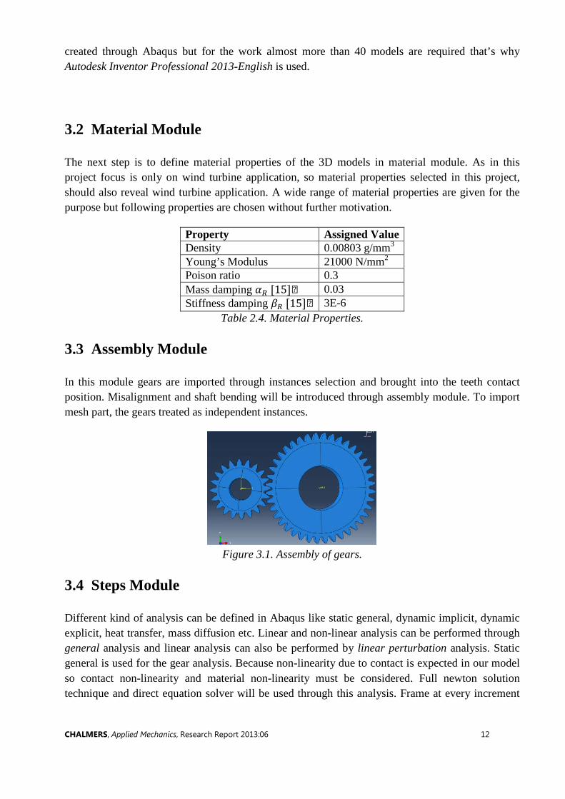
Figure 3.8.1. Dynamic force, number of elements, displacement at center and tip, and time at seed
number 0 to 01.
In appendix E 2D view of different seed number at center line of teeth is given.
It is shown from figure 3.2 that there is not much variation for dynamic force and displacement of gears. But variation for number of elements and time is higher comparatively.
Seed number 0.5 is assigned to all over the teeth. Seed number over whole gear body is 01 because it will not severely affect the results.
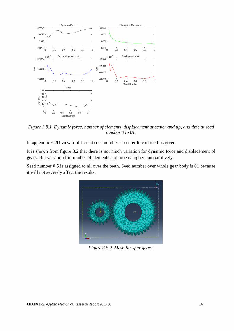
Figure 3.8.2. Mesh for spur gears.
0 0.2 0.4 0.6 0.8 12.0728
2.073
2.0732
2.0734Dynamic Force
N
0 0.2 0.4 0.6 0.8 16000
8000
10000
12000Number of Elements
0 0.2 0.4 0.6 0.8 12.6941
2.6942
2.6942x 10
-5 Centre displacement
rad
0 0.2 0.4 0.6 0.8 14.6366
4.6367
4.6368
4.6368x 10
-3 Tip displacement
rad
Seed Number
0 0.2 0.4 0.6 0.8 168
1012141618
Time
min
utes
Seed Number

CHALMERS, Applied Mechanics, Research Report 2013:06 15
Figure 3.8.3. Mesh for helical gears.
Figure 3.8.4. Mesh for planetary gears.

CHALMERS, Applied Mechanics, Research Report 2013:06 16
4 Meta-Modeling
4.1 Regression Analysis
Since full 3D finite element simulations are impractical to estimate the transmission error in drive train analysis, we aim at developing a mathematical expression of transmission error. Through this short form of mathematics it would be easy to infer about the gear running process in terms of transmission error.
A mathematical model through the regression analysis is developed between independent input variables and dependent output variables. Input variables can also be classified into two different types of variables. One type is referred to dynamic variables as these expect to be varied during running with applied torque, misalignment and shaft bending. Second type is static variables with gear ratio, pressure angle and addendum. Once gear is manufactured, its geometric parameters cannot be changed. Misalignment, shaft bending, applied torque, gear ratio; pressure angle and addendum are considered as input independent variables while transmission error is considered as output dependent variable.
Before starting to establish a mathematical model some basic concepts are necessary to be considered here.
4.1.1 Random Discrete Variables
Basically the mathematical model tries to find relationship between input variables and output variable. Since the relationship is approximate, output variables must be taken as random. If the number of observations (i.e. FE simulations of transmission error) includes experimental error or noise, these are considered as random variables. Results obtained from Abaqus simulation can be considered as random variables because of the simulation errors. And also the number of observations are discrete variables.
4.1.2 The Analysis of Variance
Total variation in the number of observations is measured by the quantity total sum of squares (𝑆𝑆𝑇). 𝑆𝑆𝑇 is computed by summing the squares of the deviations of observed values about their average value,
𝑦� = (𝑦1 + 𝑦2 + 𝑦3 + ⋯+ 𝑦𝑁) 𝑁⁄ ,
𝑆𝑆𝑇 = �(𝑦 − 𝑦�)2𝑁
1
𝑆𝑆𝑇 has 𝑁 − 1 degrees of freedom.
𝑆𝑆𝑇 can be divided into two parts: sum of squares due to regression analysis (𝑆𝑆𝑅) and sum of squares unaccounted by the developed mathematical expression or sum of squares of errors (𝑆𝑆𝐸).

CHALMERS, Applied Mechanics, Research Report 2013:06 17
𝑆𝑆𝑅 = �(𝑦� − 𝑦�)2𝑁
1
Deviation 𝑦� − 𝑦� is the difference between values predicted from the mathematical expression and over average of 𝑦. If 𝑝 is number of parameters in the mathematical expression, 𝑝 − 1 is the degrees of freedom of 𝑆𝑆𝑅.
𝑆𝑆𝐸 = �(𝑦 − 𝑦�)2𝑁
1
𝑁 − 𝑝 is the degrees of freedom for 𝑆𝑆𝐸.

CHALMERS, Applied Mechanics, Research Report 2013:06 18
5 Results
According to six parameters (an extra parameter of helix angle only for helical gears) in three different cases, 22 meta-models are developed as shown in table. 5.1.
Input Parameters Spur Gear Helical Gear Planetary Gear Radial Misalignment S1 H1 P1 Angular Misalginment S2 H2 P2 Torque S3 H3 P3 Combined: Radial, Angular and Torque
S4 H4 P4
Pressure Angle S5 H5 P5 Gear Ratio S6 H6 P6 Addendum S7 H7 P7 Helix angle H8
Table. 5.1. Assigning codes for meta-models.
5.1 Spur Gear
5.1.1 Radial Misalignment:S1
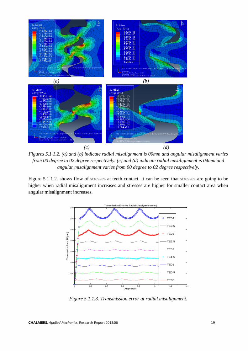
Figure 5.1.1.1. Teeth contact at 00mm radial misalignment and 00 degree angular misalignment.
CHALMERS, Applied Mechanics, Research Report 2013:06 19
(a) (b)
(c) (d)
Figures 5.1.1.2. (a) and (b) indicate radial misalignment is 00mm and angular misalignment varies from 00 degree to 02 degree respectively. (c) and (d) indicate radial misalignment is 04mm and
angular misalignment varies from 00 degree to 02 degree respectively.
Figure 5.1.1.2. shows flow of stresses at teeth contact. It can be seen that stresses are going to be higher when radial misalignment increases and stresses are higher for smaller contact area when angular misalignment increases.
Figure 5.1.1.3. Transmission error at radial misalignment.
0 0.2 0.4 0.6 0.8 1 1.2 1.40
0.01
0.02
0.03
0.04
0.05
0.06
0.07
Angle (rad)
Tran
smiss
ion
Erro
r, TE
(rad
)
Transmission Error Vs Radial Misalignment (mm)
TE04
TE3.5
TE03
TE2.5
TE02
TE1.5
TE01
TE0.5
TE00

CHALMERS, Applied Mechanics, Research Report 2013:06 20
In figure 5.1.1.3. x-axis shows angle of rotation of gears in radian and y-axis shows transmission error (TE) in radian. TE00 indicates transmission error without any misalignment and TE0.5 indicates transmission error at 0.5 mm misalignment and so on. The sinusoidal component of the transmission error has more pronounced behavior at higher misalignment than at lower misalignment. Increasing transmission error shows mean values of transmission error are increasing as shown in figure 5.1.1.4. Matlab coding to calculate transmission error is given in appendix B.
Figure 5.1.1.4. Mean of transmission error at radial misalignment.
To fit a curve to the sinusoidal form of the transmission error, four terms of sine and four terms of cosine with a mean value are taken in the following form. 𝑇𝐸 = 𝑎0 + 𝑎1 sin(2 ∗ 𝜋 ∗ 𝑓 ∗ 𝜃) + 𝑏1 cos(2 ∗ 𝜋 ∗ 𝑓 ∗ 𝜃) + 𝑎2 sin(2 ∗ 2 ∗ 𝜋 ∗ 𝑓 ∗ 𝜃)
+ 𝑏2 cos(2 ∗ 2 ∗ 𝜋 ∗ 𝑓 ∗ 𝜃) + 𝑎3 sin(3 ∗ 2 ∗ 𝜋 ∗ 𝑓 ∗ 𝜃) + 𝑏3 cos(3 ∗ 2 ∗ 𝜋 ∗ 𝑓 ∗ 𝜃)+ 𝑎4 sin(4 ∗ 2 ∗ 𝜋 ∗ 𝑓 ∗ 𝜃) + 𝑏4 cos(4 ∗ 2 ∗ 𝜋 ∗ 𝑓 ∗ 𝜃) (5.1.1.1)
Where coefficient 𝑎0 represents mean value, 𝑎1 .…𝑎4, 𝑏1…𝑏4 are coefficients of sinusoidal equation 5.1.1.1, 𝑓 is frequency and 𝜃 is the angle of rotation of pinion in radians. According to applied boundary conditions, 𝑓 is 3.159 hertz. With the frequency 3.159 Hz, TE has three periods but if numbers of periods are more than three, frequency should also be increased. It is further shown in the evaluation section of helical gears where the numbers of periods are four and for spur gears numbers of periods are three.
0 0.5 1 1.5 2 2.5 3 3.5 40
0.01
0.02
0.03
0.04
0.05
0.06
0.07
Radial Misalignment (mm)
Mea
n of
Tra
nsm
issi
on E
rror,
TE (r
ad)
Mean of Transmission Error Vs Radial Misalignment (mm)

CHALMERS, Applied Mechanics, Research Report 2013:06 21
Figure 5.1.1.5. Coefficients of sinusoidal equation for radial misalignment.
In figure 5.1.1.5. coefficient a0 is increasing which is the same behavior as in mean value of TE. Values for other coefficients are very small but these affect sinusoidal form of the TE. Now regression analysis is applied on these coefficients and gets the form as shown in table. 5.1.1.1 where coefficients are treated as output variables and radial misalignment is treated as input variable for each coefficient.
𝑎1 … 𝑎4, 𝑏1 …𝑏4 = 𝑝0 + 𝑝1𝑟 + 𝑝2𝑟2 + 𝑝3𝑟3 + 𝑝4𝑟4
Where 𝑝0,… 𝑝4 are constant terms of polynomial and 𝑟 is the value for radial misalignment.
Table. 5.1.1.1. Polynomial equations of coefficients for radial misalignment.
1 2 3 4 5 6 7 8 9-0.01
0
0.01
0.02
0.03
0.04
0.05
0.06
0.07
Radial Misalignment (mm)
coef
ficie
nts v
alue
s
Coefficients
a0a1a2a3a4b1b2b3b4
Coefficients Polynomial equations 𝑎0 0.0043 + 0.0123𝑟 + 3.8654𝑒−4𝑟2 + 6.5085𝑒−5𝑟3
− 2.4639𝑒−6𝑟4 𝑎1 −4.9772𝑒−4 − 4.72717𝑒−4𝑟 + 7.5339𝑒−4𝑟2
− 2.6949𝑒−4𝑟3 + 2.1081𝑒−5𝑟4 𝑏1 2.59039𝑒−4 + 4.62945𝑒−4𝑟 − 3.08146𝑒−4𝑟2
− 7.0794𝑒−5𝑟3 + 1.6164𝑒−5𝑟4 𝑎2 −1.43589𝑒−4 + 6.0725𝑒−4𝑟 − 3.05267𝑒−4𝑟2
+ 3.5965𝑒−5𝑟3 + 4.06877𝑒−6𝑟4 𝑏2 −8.1707𝑒−5 − 1.6136𝑒−4𝑟 + 1.2950𝑒−4𝑟2 + 8.811𝑒−6𝑟3
− 5.45328𝑒−6𝑟4 𝑎3 −2.7902𝑒−5 + 4.6452𝑒−4𝑟 − 6.0470𝑒−4𝑟2 + 2.4759𝑒−4𝑟3
− 3.2673𝑒−5𝑟4 𝑏3 6.5567𝑒−5 − 1.4127𝑒−5𝑟 + 1.3599𝑒−5𝑟2 − 1.5171𝑒−5𝑟3
+ 2.6312𝑒−6𝑟4 𝑎4 6.54256𝑒−5 − 4.49499𝑒−4𝑟 + 5.0468𝑒−4𝑟2
− 1.87818𝑒−4𝑟3 + 2.2693𝑒−5𝑟4 𝑏4 1.0805𝑒−5 + 4.3344𝑒−5𝑟 − 7.06049𝑒−5𝑟2 + 2.6319𝑒−5𝑟3
− 3.00953859616753𝑒−6𝑟4
CHALMERS, Applied Mechanics, Research Report 2013:06 22
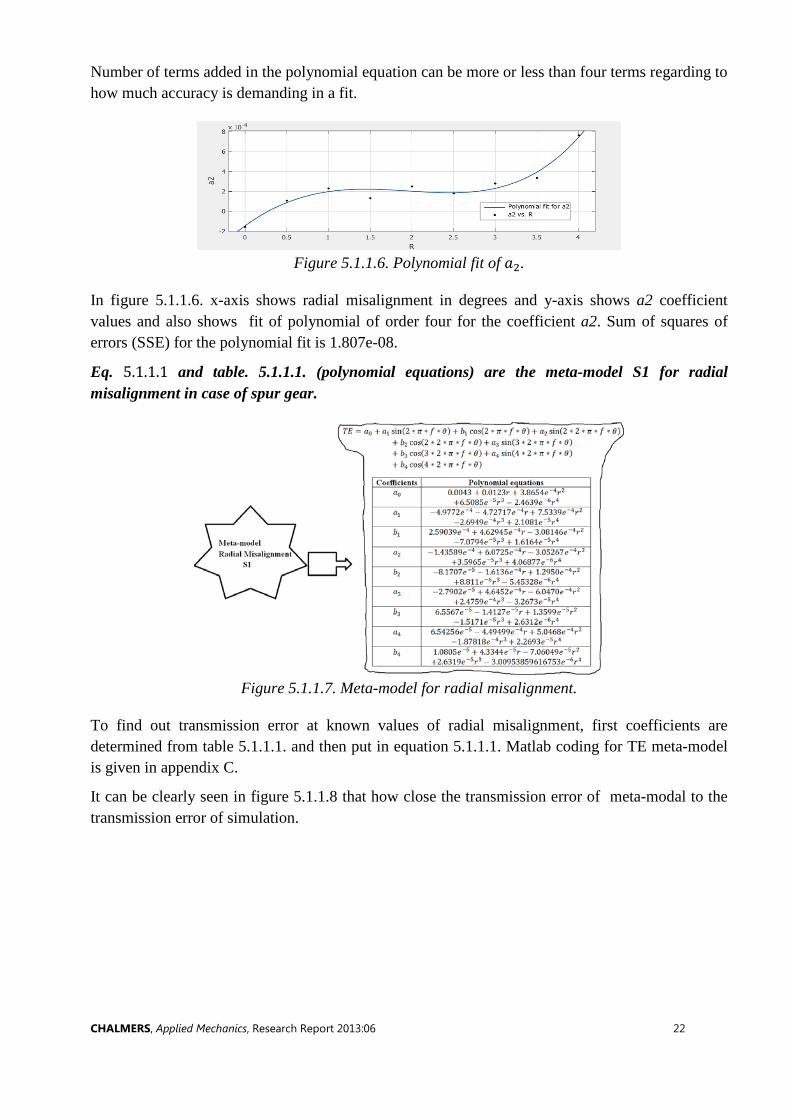
Number of terms added in the polynomial equation can be more or less than four terms regarding to how much accuracy is demanding in a fit.
Figure 5.1.1.6. Polynomial fit of 𝑎2.
In figure 5.1.1.6. x-axis shows radial misalignment in degrees and y-axis shows a2 coefficient values and also shows fit of polynomial of order four for the coefficient a2. Sum of squares of errors (SSE) for the polynomial fit is 1.807e-08.
Eq. 5.1.1.1 and table. 5.1.1.1. (polynomial equations) are the meta-model S1 for radial misalignment in case of spur gear.
Figure 5.1.1.7. Meta-model for radial misalignment.
To find out transmission error at known values of radial misalignment, first coefficients are determined from table 5.1.1.1. and then put in equation 5.1.1.1. Matlab coding for TE meta-model is given in appendix C.
It can be clearly seen in figure 5.1.1.8 that how close the transmission error of meta-modal to the transmission error of simulation.

CHALMERS, Applied Mechanics, Research Report 2013:06 23
Figure 5.1.1.8. Transmission error at 04 mm radial misalignment by meta-model and simulation.
Deviation of TE line of meta-model from TE line of simulation can be varied by changing the number of terms in sinusoidal equation and also changing the order of polynomial equations.
5.1.2. Angular Misalignment:S2
Transmission error at angular misalignment of gears till 02 degree is shown in figure 5.1.2.1.
Figure 5.1.2.1. Transmission error at angular misalignment.
In figure 5.1.2.1. x-axis shows angle of rotation of gears in radian and y-axis shows TE in radian.TE-0.2 represents that angular misalignment is 0.2 degree and TE0.4 represents that angular misalignment is 0.4 degree and so on. TE line jumps down with increased angular misalignment.
0.2 0.25 0.3 0.35 0.4 0.45 0.50.06
0.061
0.062
0.063
0.064
0.065
0.066
0.067
0.068
0.069
0.07
Angle (rad)
Tran
smiss
ion E
rror, T
E (ra
d)
Transmission Error 04 mm Radial Misalignment
Through Meta ModelThrough Simulation
0 0.2 0.4 0.6 0.8 1 1.20.008
0.01
0.012
0.014
0.016
0.018
0.02
Angle (rad)
Tran
smis
sion
Erro
r, TE
(rad
)
Transmission Error Vs Angular Misalignment (degrees)
TE-0.2
TE-0.4
TE-0.6
TE-0.8
TE-01
TE-1.2
TE-1.4
TE-1.6
TE-1.8
TE-02
CHALMERS, Applied Mechanics, Research Report 2013:06 24
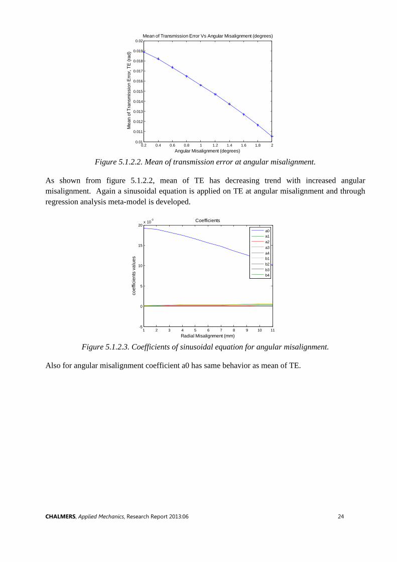
Figure 5.1.2.2. Mean of transmission error at angular misalignment.
As shown from figure 5.1.2.2, mean of TE has decreasing trend with increased angular misalignment. Again a sinusoidal equation is applied on TE at angular misalignment and through regression analysis meta-model is developed.
Figure 5.1.2.3. Coefficients of sinusoidal equation for angular misalignment.
Also for angular misalignment coefficient a0 has same behavior as mean of TE.
0.2 0.4 0.6 0.8 1 1.2 1.4 1.6 1.8 20.01
0.011
0.012
0.013
0.014
0.015
0.016
0.017
0.018
0.019
0.02
Angular Misalignment (degrees)
Mea
n of
Tra
nsm
issi
on E
rror,
TE (r
ad)
Mean of Transmission Error Vs Angular Misalignment (degrees)
1 2 3 4 5 6 7 8 9 10 11-5
0
5
10
15
20x 10
-3
Radial Misalignment (mm)
coef
ficie
nts
valu
es
Coefficients
a0a1a2a3a4b1b2b3b4

CHALMERS, Applied Mechanics, Research Report 2013:06 25
Coefficients Polynomial equations 1 r 𝑟2 𝑟3 𝑟4
𝑎0 0.0192 -9.3433 𝑒−4
-0.0048 0.0028 -6.3394 𝑒−4
𝑎1 1.0808 𝑒−4
5.2555 𝑒−4
-9.2851 𝑒−4
7.2552 𝑒−4
-1.7403 𝑒−4
𝑎2 7.0866 𝑒−5
3.0100 𝑒−4
-3.9847 𝑒−4
1.7655 𝑒−4
-1.2926 𝑒−5
𝑎3 -2.0952 𝑒−5
-1.3072 𝑒−4
1.4598 𝑒−4
-1.6466 𝑒−5
5.1038 𝑒−5
𝑎4 -1.8544 𝑒−5
-2.6782 𝑒−5
8.5839 𝑒−5
-5.4060 𝑒−5
1.1047 𝑒−5
𝑏1 1.6561 𝑒−4
7.4584 𝑒−4
-0.0013 9.6095 𝑒−4
-2.1558 𝑒−4
𝑏2 4.7686 𝑒−6
2.0798 𝑒−5
2.2442 𝑒−5
-2.9516 𝑒−5
8.3969 𝑒−6
𝑏3 -3.6873 𝑒−5
-9.2875 𝑒−5
-6.8389 𝑒−5
7.9488 𝑒−7
-2.3438 𝑒−6
𝑏4 3.0165 𝑒−5
3.9055 𝑒−4
-1.7698 𝑒−4
1.5619 𝑒−5
-4.2373 𝑒−5
Table. 5.1.2.1. Polynomial equations of coefficients for angular misalignment.
Equations of table. 5.1.2.1. and sinusoidal eq. 5.1.1.1 is the meta-model S2 for angular misalignment.
Figure 5.1.2.4. Meta-model for angular misalignment.
To find out TE at angular misalignment, first coefficients of sinusoidal equations are to be determined corresponding to angular misalignment and then substitute these values in eq. 5.1.1.1.
CHALMERS, Applied Mechanics, Research Report 2013:06 26
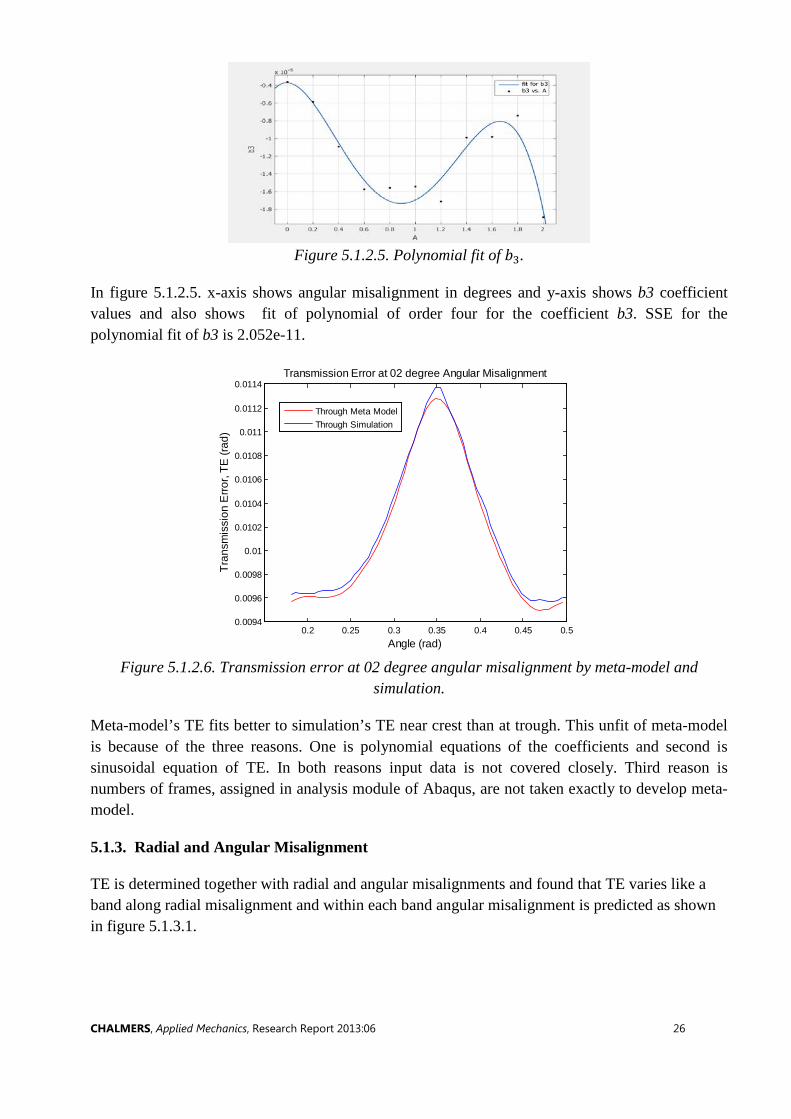
Figure 5.1.2.5. Polynomial fit of 𝑏3.
In figure 5.1.2.5. x-axis shows angular misalignment in degrees and y-axis shows b3 coefficient values and also shows fit of polynomial of order four for the coefficient b3. SSE for the polynomial fit of b3 is 2.052e-11.
Figure 5.1.2.6. Transmission error at 02 degree angular misalignment by meta-model and
simulation.
Meta-model’s TE fits better to simulation’s TE near crest than at trough. This unfit of meta-model is because of the three reasons. One is polynomial equations of the coefficients and second is sinusoidal equation of TE. In both reasons input data is not covered closely. Third reason is numbers of frames, assigned in analysis module of Abaqus, are not taken exactly to develop meta-model.
5.1.3. Radial and Angular Misalignment
TE is determined together with radial and angular misalignments and found that TE varies like a band along radial misalignment and within each band angular misalignment is predicted as shown in figure 5.1.3.1.
0.2 0.25 0.3 0.35 0.4 0.45 0.50.0094
0.0096
0.0098
0.01
0.0102
0.0104
0.0106
0.0108
0.011
0.0112
0.0114
Angle (rad)
Tran
smis
sion
Erro
r, TE
(rad
)
Transmission Error at 02 degree Angular Misalignment
Through Meta ModelThrough Simulation
CHALMERS, Applied Mechanics, Research Report 2013:06 27
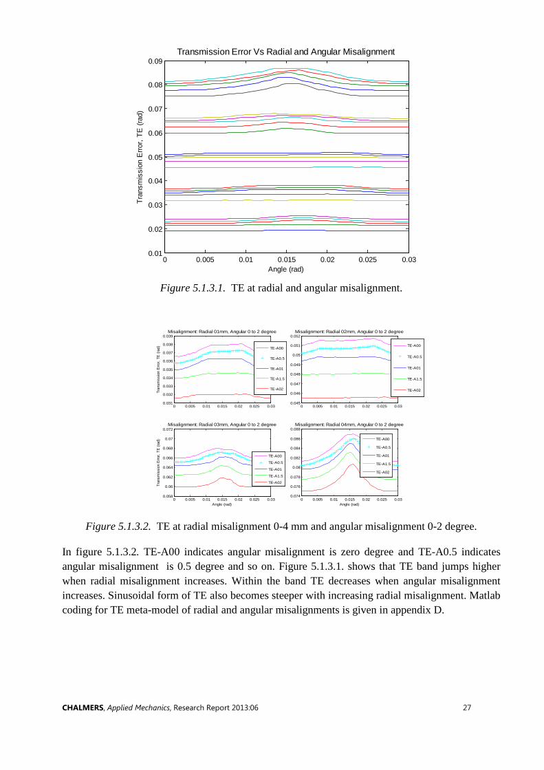
Figure 5.1.3.1. TE at radial and angular misalignment.
Figure 5.1.3.2. TE at radial misalignment 0-4 mm and angular misalignment 0-2 degree.
In figure 5.1.3.2. TE-A00 indicates angular misalignment is zero degree and TE-A0.5 indicates angular misalignment is 0.5 degree and so on. Figure 5.1.3.1. shows that TE band jumps higher when radial misalignment increases. Within the band TE decreases when angular misalignment increases. Sinusoidal form of TE also becomes steeper with increasing radial misalignment. Matlab coding for TE meta-model of radial and angular misalignments is given in appendix D.
0 0.005 0.01 0.015 0.02 0.025 0.030.01
0.02
0.03
0.04
0.05
0.06
0.07
0.08
0.09
Angle (rad)
Tran
smis
sion
Erro
r, TE
(rad
)
Transmission Error Vs Radial and Angular Misalignment
0 0.005 0.01 0.015 0.02 0.025 0.030.031
0.032
0.033
0.034
0.035
0.036
0.037
0.038
0.039
Tran
smis
sion
Erro
r, TE
(rad
)
Misalignment: Radial 01mm, Angular 0 to 2 degree
TE-A00
TE-A0.5
TE-A01
TE-A1.5
TE-A02
0 0.005 0.01 0.015 0.02 0.025 0.030.045
0.046
0.047
0.048
0.049
0.05
0.051
0.052Misalignment: Radial 02mm, Angular 0 to 2 degree
TE-A00
TE-A0.5
TE-A01
TE-A1.5
TE-A02
0 0.005 0.01 0.015 0.02 0.025 0.030.058
0.06
0.062
0.064
0.066
0.068
0.07
0.072
Angle (rad)
Tran
smis
sion
Erro
r, TE
(rad
)
Misalignment: Radial 03mm, Angular 0 to 2 degree
TE-A00
TE-A0.5
TE-A01
TE-A1.5
TE-A02
0 0.005 0.01 0.015 0.02 0.025 0.030.074
0.076
0.078
0.08
0.082
0.084
0.086
0.088
Angle (rad)
Misalignment: Radial 04mm, Angular 0 to 2 degree
TE-A00
TE-A0.5
TE-A01
TE-A1.5
TE-A02

CHALMERS, Applied Mechanics, Research Report 2013:06 28
5.1.4. Transmission error for torque:S3
(a) (b)
(c) (d) Figure 5.1.4.1 (a) and (c) teeth contact at 20 kNm torque and (b) and (d) teeth contact at 170 kNm
torque.
Form Figure 5.1.4.1 it can be seen that stresses are increased with higher torque.
Figure 5.1.4.2. Transmission error at torque (kNm).
0 0.2 0.4 0.6 0.8 1 1.2 1.40
0.5
1
1.5
2
2.5
3x 10
-3
Angle (rad)
Tran
smis
sion
Erro
r, TE
(rad
)
Transmission Error at Torque (KN.m)
TE-20
TE-30
TE-40
TE-50
TE-60
TE-70
TE-80
TE-90
TE-100
TE-110
TE-120
TE-130
TE-140
TE-150
TE-160
TE-170
TE-180
CHALMERS, Applied Mechanics, Research Report 2013:06 29
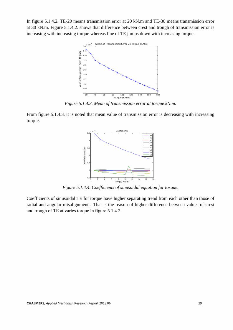
In figure 5.1.4.2. TE-20 means transmission error at 20 kN.m and TE-30 means transmission error at 30 kN.m. Figure 5.1.4.2. shows that difference between crest and trough of transmission error is increasing with increasing torque whereas line of TE jumps down with increasing torque.
Figure 5.1.4.3. Mean of transmission error at torque kN.m.
From figure 5.1.4.3. it is noted that mean value of transmission error is decreasing with increasing torque.
Figure 5.1.4.4. Coefficients of sinusoidal equation for torque.
Coefficients of sinusoidal TE for torque have higher separating trend from each other than those of radial and angular misalignments. That is the reason of higher difference between values of crest and trough of TE at varies torque in figure 5.1.4.2.
20 40 60 80 100 120 140 160 1800.6
0.8
1
1.2
1.4
1.6
1.8
2
2.2
2.4
2.6x 10
-3
Torque (KN.m)
Mea
n of
Tra
nsm
issio
n Er
ror,
TE (r
ad)
Mean of Transmission Error Vs Torque (KN.m)
0 2 4 6 8 10 12 14 16 18-0.5
0
0.5
1
1.5
2
2.5x 10
-3
Torque KN/m
coef
ficie
nts
valu
es
Coefficients
a0a1a2a3a4b1b2b3b4

CHALMERS, Applied Mechanics, Research Report 2013:06 30
Coefficients Polynomial equations 1 r 𝑟2 𝑟3 𝑟4
𝑎0 0.0031 -3.7459 𝑒−5
3.765 𝑒−7
-2.1476 𝑒−9
4.5072 𝑒−12
𝑎1 4.1592 𝑒−4
-2.8551 𝑒−5
4.5866 𝑒−7
-2.9523 𝑒−9
6.3348 𝑒−12
𝑎2 1.2816 𝑒−4
-7.6206 𝑒−6
1.1468 𝑒−7
-7.0347 𝑒−10
1.4407 𝑒−12
𝑎3 -1.8782 𝑒−5
1.4109 𝑒−6
-2.4326 𝑒−8
1.5908 𝑒−10
-3.3721 𝑒−13
𝑎4 6.9823 𝑒−5
-4.9697 𝑒−6
8.1261 𝑒−8
-5.1606 𝑒−10
1.113 𝑒−12
𝑏1 6.0342 𝑒−5
-5.1068 𝑒−6
5.20 𝑒−8
-2.8162 𝑒−10
5.6079 𝑒−13
𝑏2 -3.199 𝑒−5
2.8319 𝑒−6
-3.3325 𝑒−8
-2.0566 𝑒−10
-4.5483 𝑒−13
𝑏3 1.9874 𝑒−5
-2.2237 𝑒−6
3.6242 𝑒−8
-2.3896 𝑒−10
5.5406 𝑒−13
𝑏4 1.8903 𝑒−5
-8.8718 𝑒−7
8.0283 𝑒−9
-2.2977 𝑒−11
2.6732 𝑒−15
Table. 5.1.4.1. Polynomial equations of coefficients for torque.
Figure 5.1.4.5. Polynomial fit of 𝑏3.
In figure 5.1.4.5. x-axis shows torque in kN and y-axis shows b3 coefficient values and also shows fit of polynomial of order four for the coefficient b3. SSE of polynomial fit for torque is 6.784e-12.

CHALMERS, Applied Mechanics, Research Report 2013:06 31
Figure 5.1.4.6. Meta-model for torque.
Figure 5.1.4.7. Transmission error at 180 kNm by meta-model and simulation.
Figure 5.1.4.7. shows TE line for torque from meta-model covers closely the TE from Abaqus simulation rather than variation within crest. Meta-model developed in this project cannot cover efficiently variations within crest or within trough. These kinds of variations are also tried to cover through polynomial order but that is not sufficient for the variations within crest or within trough.
5.1.5. Transmission error for radial, angular, and torque:S4
Combined effects of radial, angular and torque are determined by adding the coefficients of three meta-models. Because of the addition of coefficients, the dynamic parameters are considered independent to each other in combined effect of transmission error. But in real applications the dynamic parameters are dependent to each other.
0.05 0.1 0.15 0.2 0.25 0.3 0.35 0.40
0.2
0.4
0.6
0.8
1
1.2x 10
-3
Torque (KN.m)
Mea
n of
Tra
nsm
issi
on E
rror,
TE (r
ad)
Through Meta ModelThrough Simulation

CHALMERS, Applied Mechanics, Research Report 2013:06 32
Figure 5.1.5.1. Combine effect of radial and angular misalignment and torque.
Figure 5.1.5.1. shows TE at radial misalignment, angular misalignment and torque. Radial misalignment contributes more to TE than angular misalignment and torque. Radial misalignment tries to increase TE whereas angular misalignment and increasing torque try to decrease TE.
5.1.6. Transmission error for pressure angle:S5
(a) (b)
(c) (d)
Figure 5.1.6.1. (a) and (c) teeth contact at 15 degree pressure angle and, (b) and (d) teeth contact at 15 degree pressure angle.
Figure 5.1.6.1. shows stresses at 15 degree pressure angle are lower than at 35 degree pressure angle.
0.2 0.25 0.3 0.35 0.4 0.45 0.50.06
0.062
0.064
0.066
0.068
0.07TE at 04 mm radial misalignment
TE (r
ad)
0.2 0.25 0.3 0.35 0.4 0.45 0.50.0095
0.01
0.0105
0.011
0.0115TE at 02 degree angular misalignment
0.2 0.25 0.3 0.35 0.4 0.45 0.50
0.2
0.4
0.6
0.8
1
1.2x 10
-3 TE at 180 KN.m torque
TE (r
ad)
Angle (rad)0.2 0.25 0.3 0.35 0.4 0.45 0.5
0.07
0.072
0.074
0.076
0.078
0.08TE at 04 mm radial and 02 degree angular and at 180 KN.m torque
Angle (rad)

CHALMERS, Applied Mechanics, Research Report 2013:06 33
Figure 5.1.6.2. Transmission error at pressure angle.
Figure 5.1.6.2 shows TE line at increasing pressure angle values jumps ups and downs.
Figure 5.1.6.3. Coefficients of sinusoidal equation for pressure angle.
Figure 5.1.6.3. shows behavior of coefficients of sinusoidal equation for pressure angle. Coefficient a0 shows that mean value of TE goes ups and downs when pressure angle is increasing. Separation and variation of rest of coefficients accounts for variation of sinusoidal form of TE.
Figure 5.1.6.4. Polynomial fit of 𝑏4.
0 0.2 0.4 0.6 0.8 1 1.2 1.4-8
-6
-4
-2
0
2
4
6x 10
-3
Angle (rad)
Tran
smis
sion
Erro
r, TE
(rad
)
Transmission Error at Pressure Angle
TE 15
TE 20
TE 25
TE 23
TE 30
TE 35
15 20 25 30 35-6
-4
-2
0
2
4
6x 10
-3
Pressure Angle (degrees)
coef
ficie
nts
valu
es
Coefficients
a0a1a2a3a4b1b2b3b4

CHALMERS, Applied Mechanics, Research Report 2013:06 34
In figure 5.1.6.4. x-axis shows pressure angle in degrees and y-axis shows b4 coefficient values and also shows fit of polynomial of order four for the coefficient b4. SSE of polynomial fit for pressure angle is 7.62e-10.
Figure 5.1.6.5. Transmission error at 35 degree pressure anlge by meta-model and simulation.
In figure 5.1.6.5. TE measured from meta-model is closely fit TE measured from simulation.
5.1.7. Transmission error for gear ratio:S6
(a) (b)
(c) (d)
Figure 5.1.7.1. (a) and (c) Teeth contact at gear ratio 5.5 and (b) and (d) teeth contact at gear ratio 01.
Figure 5.1.7.1. shows flow of stresses at gear ratio 5.5 and 01.
0.2 0.25 0.3 0.35 0.4 0.45 0.5 0.55-2.5
-2
-1.5
-1
-0.5
0
0.5
1
1.5
2
2.5x 10
-3
Angle (rad)
Tran
smiss
ion E
rror, T
E (ra
d)
Transmission Error at 35 degree pressure angle
Through Meta ModelThrough Simulation

CHALMERS, Applied Mechanics, Research Report 2013:06 35
Figure 5.1.7.2. Transmission error at gear ratio.
TE line for gear ratio is also jumps ups and downs with increasing gear ratio.
Figure 5.1.7.3. Mean of transmission error at gear ratio.
In figure 5.1.7.3 mean of TE jumps up and down.
Figure 5.1.7.4. Transmission error at gear ratio 01 by meta-model and simulation.
Figure 5.1.7.4 shows TE line of meta-model is not closely fit to TE line of simulation. Meta-model of gear ratio for spur gears is not a good prediction of TE. That might be due to simulation errors.
0 0.2 0.4 0.6 0.8 1 1.2 1.4-0.015
-0.01
-0.005
0
0.005
0.01
Angle (rad)
Tran
smis
sion
Erro
r, TE
(rad
)
Transmission Error at Gear Ratio
TE 01
TE 1.5
TE 2
TE 2.5
TE 3
TE 3.5
TE 4
TE 5
TE 5.5
TE 6
1 1.5 2 2.5 3 3.5 4 4.5 5 5.5 6-9
-8
-7
-6
-5
-4
-3
-2
-1
0
1x 10
-3
Gear Ratio
Mea
n of T
ransm
ission
Erro
r, TE
(rad)
Mean of Transmission Error Vs Gear Ratio
0 10 20 30 40 50 60 702
3
4
5
6
7
8
9
10x 10
-3
Angle (rad)
Tran
smiss
ion E
rror, T
E (ra
d)
Transmission Error at Gear Ratio
Through Meta ModelThrough Simulation

CHALMERS, Applied Mechanics, Research Report 2013:06 36
5.1.8. Transmission error for addendum:S7
(a) (b)
(c) (d)
Figure 5.1.8.1. (a) and (c) Teeth contact at addendum 0.4 and (b) and (d) teeth contact at addendum 1.2.
Figure 5.1.8.1. shows stresses at addendum 0.4 mm are lower than at 1.2 mm. And also stresses are higher at higher addendum value than at lower addendum value. At higher addendum value teeth contact is higher than at lower addendum value.
Figure 5.1.8.2. Transmission error at addendum.
In figure 5.1.8.2. TE line jumps up with increasing addendum value of gears.
0 0.2 0.4 0.6 0.8 1 1.2 1.4-0.03
-0.025
-0.02
-0.015
-0.01
-0.005
0
0.005
0.01
0.015
Angle (rad)
Tran
smiss
ion E
rror, T
E (ra
d)
Transmission Error at Addendum (mm)
TE-1p2
TE-1p1
TE-01
TE-0p8
TE-0p9
TE-0p6
TE-0p4

CHALMERS, Applied Mechanics, Research Report 2013:06 37
Figure 5.1.8.3. Coefficients of sinusoidal equation for addendum.
In figure 5.1.8.3. a0 is also increasing with increased addendum values and separation between the coefficients account for sinusoidal form. For addendum of gears, a0 has same increasing trend as mean value of TE lines.
Figure 5.1.8.4. Polynomial fit of 𝑎0.
In figure 5.1.8.4. x-axis shows addendum in millimeter and y-axis shows a0 coefficient values and also shows fit of polynomial of order four for the coefficient a0. SSE of polynomial fit for addendum is 2.172e-32.
Figure 5.1.8.5. Transmission error at 0.8 mm addendum by meta-model and simulation.
0.4 0.5 0.6 0.7 0.8 0.9 1-0.025
-0.02
-0.015
-0.01
-0.005
0
0.005
Addendum
coeff
icien
ts va
lues
Coefficients
a0a1a2a3a4b1b2b3b4
0.2 0.25 0.3 0.35 0.4 0.45 0.5 0.55-8
-7
-6
-5
-4
-3
-2
-1
0
1x 10
-3
Angle (rad)
Tran
smis
sion
Erro
r, TE
(rad
)
Transmission Error at 0.8 mm Addendum
Through Meta ModelThrough Simulation

CHALMERS, Applied Mechanics, Research Report 2013:06 38
Figure 5.1.8.5. shows that TE of meta-model can fit into the sinusoidal form but it cannot fit into the variations within the sinusoidal form.
5.2 Helical Gear
5.2.1 Radial Misalignment:H1
Transmission error variations for helical gear behave almost in the same manner as in spur gear for radial misalignment.
Figure 5.2.1.1. Transmission error at radial misalignment.
In case of spur gear two trends are found with increased radial misalignment. One is increasing mean value of TE and second is sinusoidal form which is going to be steeper. But in case of helical gears only mean value of TE is increasing with increased radial misalignment as shown in figure 5.2.1.1.
0 0.2 0.4 0.6 0.8 1 1.2 1.4-0.01
0
0.01
0.02
0.03
0.04
0.05
0.06
Angle (rad)
Tran
smis
sion
Erro
r, TE
(rad
)
Transmission Error Vs Radial Misalignment (mm)
TE03
TE2.5
TE02
TE1.5
TE01
TE0.5
TE00
CHALMERS, Applied Mechanics, Research Report 2013:06 39
Figure 5.2.1.2. Coefficients of sinusoidal equation for radial misalignment.
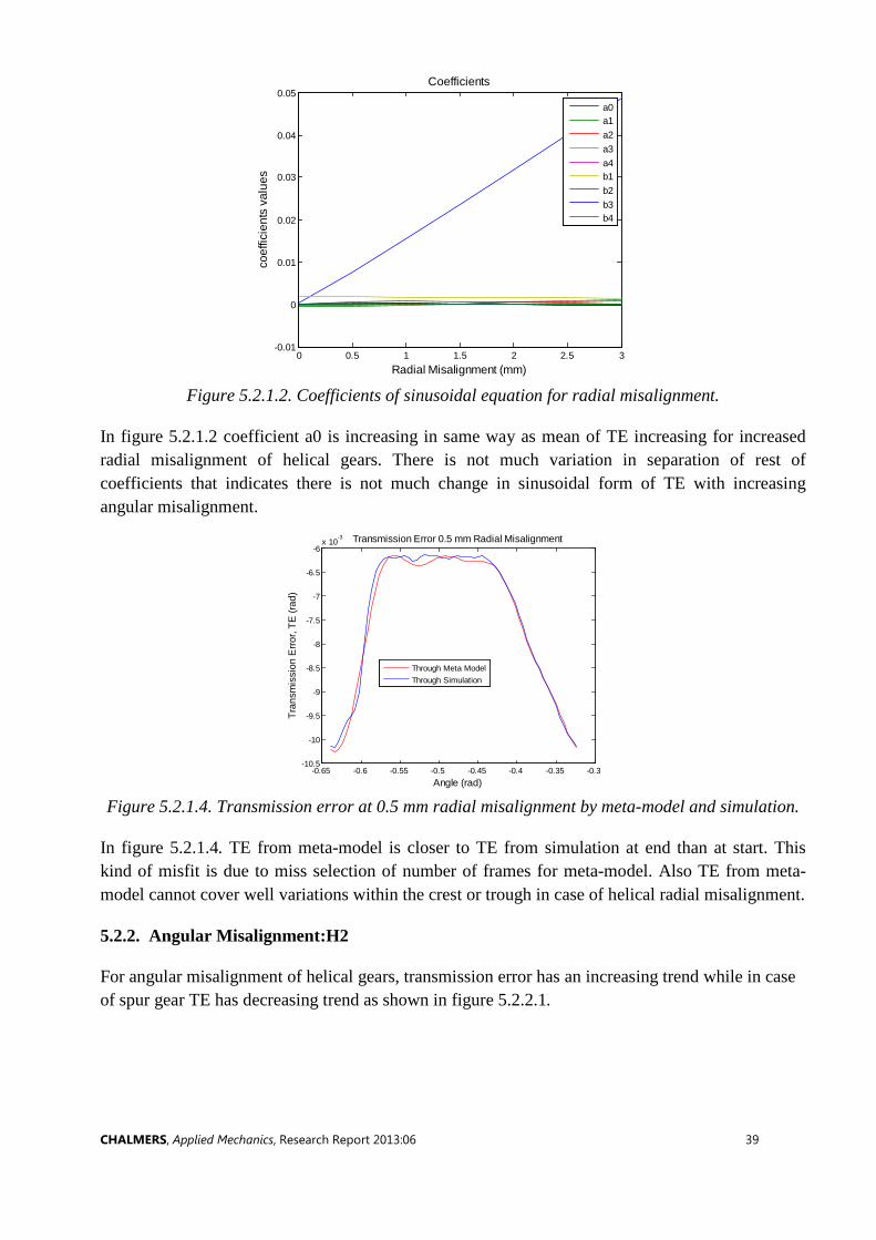
In figure 5.2.1.2 coefficient a0 is increasing in same way as mean of TE increasing for increased radial misalignment of helical gears. There is not much variation in separation of rest of coefficients that indicates there is not much change in sinusoidal form of TE with increasing angular misalignment.
Figure 5.2.1.4. Transmission error at 0.5 mm radial misalignment by meta-model and simulation.
In figure 5.2.1.4. TE from meta-model is closer to TE from simulation at end than at start. This kind of misfit is due to miss selection of number of frames for meta-model. Also TE from meta-model cannot cover well variations within the crest or trough in case of helical radial misalignment.
5.2.2. Angular Misalignment:H2
For angular misalignment of helical gears, transmission error has an increasing trend while in case of spur gear TE has decreasing trend as shown in figure 5.2.2.1.
0 0.5 1 1.5 2 2.5 3-0.01
0
0.01
0.02
0.03
0.04
0.05
Radial Misalignment (mm)
coef
ficie
nts
valu
es
Coefficients
a0a1a2a3a4b1b2b3b4
-0.65 -0.6 -0.55 -0.5 -0.45 -0.4 -0.35 -0.3-10.5
-10
-9.5
-9
-8.5
-8
-7.5
-7
-6.5
-6x 10
-3
Angle (rad)
Tran
smis
sion
Erro
r, TE
(rad
)
Transmission Error 0.5 mm Radial Misalignment
Through Meta ModelThrough Simulation

CHALMERS, Applied Mechanics, Research Report 2013:06 40
Figure 5.2.2.1. Transmission error at angulr misalignment.
Figure 5.2.2.2. Mean of transmission error at angular misalignment.
In figure 5.2.2.2. mean of TE is increasing with increased angular misalignment. The increasing trend is not consistent and this inconsistency is likely due to simulation errors in Abaqus.
0 0.1 0.2 0.3 0.4 0.5 0.6 0.7 0.8 0.9 10.015
0.02
0.025
0.03
0.035
0.04
Angle (rad)
Tran
smis
sion
Erro
r, TE
(rad
)
Transmission Error Vs Angular Misalignment (degrees)
TE-02TE-1.8TE-1.6TE-1.4TE-1.2TE-01TE-0.8TE-0.6TE-0.4TE-0.2
0 0.2 0.4 0.6 0.8 1 1.2 1.4 1.6 1.8 20.022
0.023
0.024
0.025
0.026
0.027
0.028
0.029
0.03
Angular Misalignment (degrees)
Mea
n of
Tra
nsm
issi
on E
rror,
TE (r
ad)
Mean of Transmission Error Vs Angular Misalignment (degrees)
CHALMERS, Applied Mechanics, Research Report 2013:06 41
Figure 5.2.2.3. Transmission error at 0.4 degree angular misalignment by meta-model and
simulation.
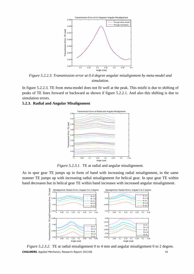
In figure 5.2.2.3. TE from meta-model does not fit well at the peak. This misfit is due to shifting of peaks of TE lines forward or backward as shown if figure 5.2.2.1. And also this shifting is due to simulation errors. 5.2.3. Radial and Angular Misalignment
Figure 5.2.3.1. TE at radial and angular misalignment.
As in spur gear TE jumps up in form of band with increasing radial misalignment, in the same manner TE jumps up with increasing radial misalignment for helical gear. In spur gear TE within band decreases but in helical gear TE within band increases with increased angular misalignment.
Figure 5.2.3.2. TE at radial misalignment 0 to 4 mm and angular misalignment 0 to 2 degree.
0.2 0.25 0.3 0.35 0.4 0.45 0.50.022
0.023
0.024
0.025
0.026
0.027
0.028
0.029
Angle (rad)
Tran
smis
sion
Erro
r, TE
(rad
)
Transmission Error at 0.4 degrees Angular Misalignment
Through Meta ModelThrough Simulation
0 0.05 0.1 0.15 0.2 0.25 0.3 0.350
0.01
0.02
0.03
0.04
0.05
0.06
0.07
0.08
Angle (rad)
Tran
smis
sion
Erro
r, TE
(rad
)
Transmission Error at Radial and Angular Misalignment
0 0.05 0.1 0.15 0.2 0.25 0.3 0.350.015
0.02
0.025
0.03
Tran
smis
sion
Erro
r, TE
(rad
)
Misalignment: Radial 01mm, Angular 0 to 2 degree
TE-02TE-1.5TE-01TE-0.5TE-00
0 0.05 0.1 0.15 0.2 0.25 0.3 0.350.03
0.035
0.04
0.045Misalignment: Radial 02mm, Angular 0 to 2 degree
TE-02TE-1.5TE-01TE-0.5TE-00
0 0.05 0.1 0.15 0.2 0.25 0.3 0.350.05
0.055
0.06
0.065
Angle (rad)Tran
smis
sion
Erro
r, TE
(rad
)
TE-02TE-1.5TE-01TE-0.5TE-00
0 0.05 0.1 0.15 0.2 0.25 0.3 0.350.055
0.06
0.065
0.07
0.075
0.08
Angle (rad)
TE-02TE-1.5TE-01TE-0.5TE-00

CHALMERS, Applied Mechanics, Research Report 2013:06 42
From band to band there is also a little increase in sinusoidal form of TE as shown in figure 5.2.3.2.
5.2.6. Transmission error for torque:H3
Transmission error lines jumps down for torque in helical gear as in spur gear but with steeper trend as shown in figure 5.2.6.1.
Figure 5.2.6.1. Transmission error at torque (kNm).
Figure 5.2.4.2. Coefficients of sinusoidal equation for torque.
In figure 5.2.4.2. coefficient a0 has decreasing trend with increased torque and coefficient b1 has large value which brings it far from other coefficients. This separation of b1 accounts more for sinusoidal form than other coefficients.
0 0.2 0.4 0.6 0.8 1 1.2 1.4-6
-5
-4
-3
-2
-1
0
1
2
3x 10
-3
Angle (rad)
Tran
smis
sion
Erro
r, TE
(rad
)
Transmission Error at Torque (KN.m)
TE-01TE-05TE-10TE-20TE-30TE-40TE-50TE-60TE-70TE-80TE-90TE-100TE-110TE-120TE-130TE-140TE-150TE-160TE-170TE-180
0 2 4 6 8 10 12 14 16 18 20-4
-3
-2
-1
0
1
2
3x 10
-3
Torque KN.m
coef
ficie
nts
valu
es
Coefficients
a0a1a2a3a4b1b2b3b4

CHALMERS, Applied Mechanics, Research Report 2013:06 43
Figure 5.2.2.3. Transmission error at 120 kNm by meta-model and simulation.
TE of meta-model is closely fit with TE of simulation in figure 5.2.2.3.
5.2.5. Transmission error for radial, angular misalignments and torque:H4 Combined effects of radial misalignment, angular misalignment and torque are determined by adding the coefficients of three meta-models. Again the dynamic parameters are considered independent to each other.
Figure 5.2.5.1. Combine effect of radial and angular misalignments and torque.
In figure 5.2.5.1 a combined TE of radial and angular misalignments and torque, radial and angular misalignments have dominant effect than torque whereas in spur gear only radial misalignment has dominant effect. Radial and angular misalignments try to increase TE whereas torque tries to decrease TE. Torque tries to increase sinusoidal form of TE.
0.35 0.4 0.45 0.5 0.55 0.6 0.65 0.70.5
1
1.5
2
2.5
3
3.5
4
4.5
5x 10
-3
Angle (rad)Tr
ansm
issi
on E
rror,
TE (r
ad)
Transmission Error at 120 KN.m Torque
Through Meta ModelThrough Simulation
0.2 0.25 0.3 0.35 0.4 0.45 0.50.0306
0.0308
0.031
0.0312
0.0314
0.0316
0.0318TE at 02 mm radial misalignment
TE (r
ad)
0.2 0.25 0.3 0.35 0.4 0.45 0.50.0152
0.0154
0.0156
0.0158
0.016
0.0162TE at 01 degree angular misalignment
0.2 0.25 0.3 0.35 0.4 0.45 0.51.2
1.3
1.4
1.5
1.6
1.7
1.8x 10
-3 TE at 90 KN.m torque
TE (r
ad)
Angle (rad)0.2 0.25 0.3 0.35 0.4 0.45 0.5
0.0476
0.0478
0.048
0.0482
0.0484
0.0486
0.0488TE at 04 mm radial and 02 degree angular and at 180 KN.m torque
Angle (rad)
CHALMERS, Applied Mechanics, Research Report 2013:06 44
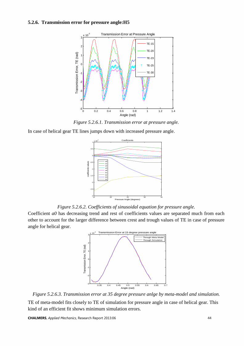
5.2.6. Transmission error for pressure angle:H5
Figure 5.2.6.1. Transmission error at pressure angle.
In case of helical gear TE lines jumps down with increased pressure angle.
Figure 5.2.6.2. Coefficients of sinusoidal equation for pressure angle.
Coefficient a0 has decreasing trend and rest of coefficients values are separated much from each other to account for the larger difference between crest and trough values of TE in case of pressure angle for helical gear.
Figure 5.2.6.3. Transmission error at 35 degree pressure anlge by meta-model and simulation.
TE of meta-model fits closely to TE of simulation for pressure angle in case of helical gear. This kind of an efficient fit shows minimum simulation errors.
0 0.2 0.4 0.6 0.8 1 1.2 1.4-5
-4
-3
-2
-1
0
1
2
3x 10
-3
Angle (rad)
Tran
smis
sion
Erro
r, TE
(rad
)
Transmission Error at Pressure Angle
TE-15
TE-20
TE-23
TE-25
TE-30
15 20 25 30 35-3
-2.5
-2
-1.5
-1
-0.5
0
0.5
1x 10
-3
Pressure Angle (degrees)
coef
ficie
nts v
alue
s
Coefficients
a0a1a2a3a4b1b2b3b4
0.35 0.4 0.45 0.5 0.55 0.6 0.65 0.7-3
-2
-1
0
1
2
3x 10
-3
Angle (rad)
Tran
smiss
ion E
rror, T
E (ra
d)
Transmission Error at 15 degree pressure angle
Through Meta ModelThrough Simulation

CHALMERS, Applied Mechanics, Research Report 2013:06 45
5.2.7. Transmission error for gear ratio:H6
Figure 5.2.7.1. Transmission error at gear ratio.
TE line jumps up and down with increased gear ratio for helical gear.
Figure 5.2.7.2. Mean of TE for gear ratio.
Mean of TE jumps up and down with increased gear ratio.
Figure 5.2.7.3. Transmission error at 5 gear ratio by meta-model and simulation.
0 0.2 0.4 0.6 0.8 1 1.2 1.4-4
-3
-2
-1
0
1
2
3
4x 10
-3
Angle (rad)
Tran
smis
sion
Erro
r, TE
(rad
)
Transmission Error at Gear Ratio
TE 01
TE 02
TE 1.5
TE 03
TE 3.5
TE 04
TE 4.5
TE 2.5
TE 05
1 1.5 2 2.5 3 3.5 4 4.5 5-2
-1.5
-1
-0.5
0
0.5
1x 10
-3
Gear Ratio
Mea
n of
Tra
nsm
issio
n Er
ror,
TE (r
ad)
Mean of Transmission Error Vs Gear Ratio
0.35 0.4 0.45 0.5 0.55 0.6 0.65 0.7-4
-3.5
-3
-2.5
-2
-1.5
-1
-0.5
0
0.5x 10
-3
Angle (rad)
Tran
smis
sion
Erro
r, TE
(rad
)
Transmission Error at 5 Gear Ratio
Through Meta ModelThrough Simulation
CHALMERS, Applied Mechanics, Research Report 2013:06 46
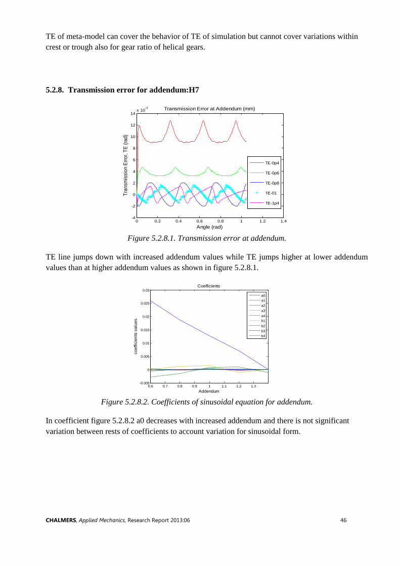
TE of meta-model can cover the behavior of TE of simulation but cannot cover variations within crest or trough also for gear ratio of helical gears. 5.2.8. Transmission error for addendum:H7
Figure 5.2.8.1. Transmission error at addendum.
TE line jumps down with increased addendum values while TE jumps higher at lower addendum values than at higher addendum values as shown in figure 5.2.8.1.
Figure 5.2.8.2. Coefficients of sinusoidal equation for addendum.
In coefficient figure 5.2.8.2 a0 decreases with increased addendum and there is not significant variation between rests of coefficients to account variation for sinusoidal form.
0 0.2 0.4 0.6 0.8 1 1.2 1.4-4
-2
0
2
4
6
8
10
12
14x 10
-3
Angle (rad)
Tran
smis
sion
Erro
r, TE
(rad
)
Transmission Error at Addendum (mm)
TE-0p4
TE-0p6
TE-0p8
TE-01
TE-1p4
0.6 0.7 0.8 0.9 1 1.1 1.2 1.3-0.005
0
0.005
0.01
0.015
0.02
0.025
0.03
Addendum
coef
ficie
nts
valu
es
Coefficients
a0a1a2a3a4b1b2b3b4
CHALMERS, Applied Mechanics, Research Report 2013:06 47
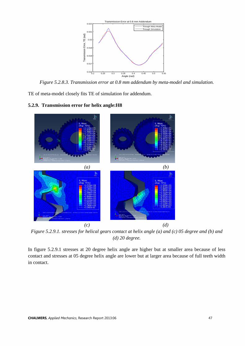
Figure 5.2.8.3. Transmission error at 0.8 mm addendum by meta-model and simulation.
TE of meta-model closely fits TE of simulation for addendum.
5.2.9. Transmission error for helix angle:H8
(a) (b)
(c) (d)
Figure 5.2.9.1. stresses for helical gears contact at helix angle (a) and (c) 05 degree and (b) and (d) 20 degree.
In figure 5.2.9.1 stresses at 20 degree helix angle are higher but at smaller area because of less contact and stresses at 05 degree helix angle are lower but at larger area because of full teeth width in contact.
0.2 0.25 0.3 0.35 0.4 0.45 0.5 0.550.016
0.017
0.018
0.019
0.02
0.021
0.022
Angle (rad)
Tran
smiss
ion
Erro
r, TE
(rad
)
Transmission Error at 0.8 mm Addendum
Through Meta ModelThrough Simulation

CHALMERS, Applied Mechanics, Research Report 2013:06 48
Figure 5.2.9.2. Transmission error at helix angle.
TE line of helical gears is also jumps down with increased helix except TE line at 20 degree pressure angle. That unexpected behavior is also due to simulation errors.
Figure 5.2.9.3. Coefficients of sinusoidal equation for helix angle.
In figure 5.2.9.3 mean of TE indicates same behavior as TE jumps.
0 0.2 0.4 0.6 0.8 1 1.2 1.4-16
-14
-12
-10
-8
-6
-4
-2
0
2
4x 10
-3
Angle (rad)
Tran
smis
sion
Erro
r, TE
(rad
)
Transmission Error at Helix Angle (degrees)
TE 05
TE 10
TE 15
TE 20
TE 25
5 10 15 20 25-0.015
-0.01
-0.005
0
Helix Angle (degree)
Mea
n of
Tra
nsm
issi
on E
rror,
TE (r
ad)
Mean of Transmission Error Vs Helix Angle (degree)
0.2 0.25 0.3 0.35 0.4 0.45 0.5 0.55-8
-7.5
-7
-6.5
-6
-5.5
-5x 10
-3
Angle (rad)
Tran
smis
sion
Erro
r, TE
(rad
)
Transmission Error at 25 degree Helix Angle
Through Meta ModelThrough Simulation

CHALMERS, Applied Mechanics, Research Report 2013:06 49
Figure 5.2.9.4. Transmission error at 25 degree helix angle by meta-model and simulation.
TE of meta-model is also very close to TE of simulation for helix angle.
5.3 Planetary Gear
5.3.1. Radial and Angular Misalignment
(a) (b)
(c) (d) Figure 5.3.1.1. stresses for planetary gears contact at radial misalignment (a) and (c) 00 mm and
(b) and (d) 03 mm.
In figure 5.3.1.1 stresses at 00 mm radial misalignment are lower and stresses at 03 mm radial misalignment are higher.
CHALMERS, Applied Mechanics, Research Report 2013:06 50
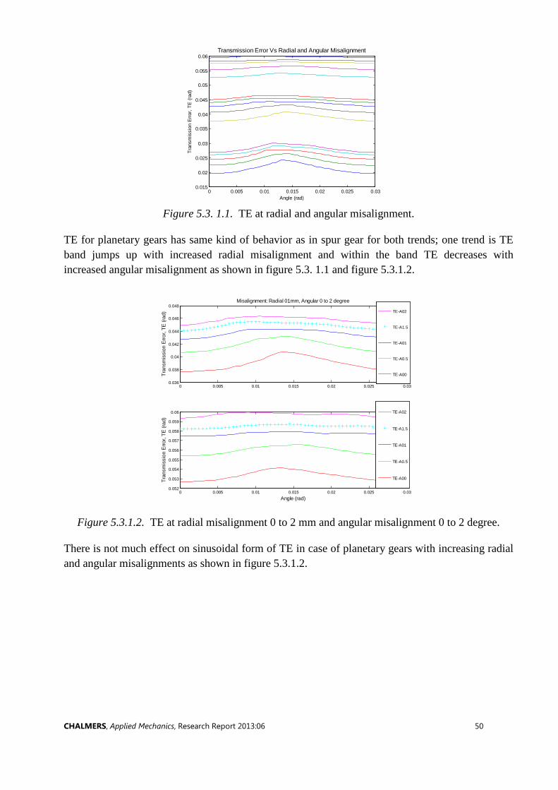
Figure 5.3. 1.1. TE at radial and angular misalignment.
TE for planetary gears has same kind of behavior as in spur gear for both trends; one trend is TE band jumps up with increased radial misalignment and within the band TE decreases with increased angular misalignment as shown in figure 5.3. 1.1 and figure 5.3.1.2.
Figure 5.3.1.2. TE at radial misalignment 0 to 2 mm and angular misalignment 0 to 2 degree.
There is not much effect on sinusoidal form of TE in case of planetary gears with increasing radial and angular misalignments as shown in figure 5.3.1.2.
0 0.005 0.01 0.015 0.02 0.025 0.030.015
0.02
0.025
0.03
0.035
0.04
0.045
0.05
0.055
0.06
Angle (rad)
Tran
smis
sion
Erro
r, TE
(rad
)
Transmission Error Vs Radial and Angular Misalignment
0 0.005 0.01 0.015 0.02 0.025 0.030.036
0.038
0.04
0.042
0.044
0.046
0.048
Tran
smis
sion
Erro
r, TE
(rad
)
Misalignment: Radial 01mm, Angular 0 to 2 degree
TE-A02
TE-A1.5
TE-A01
TE-A0.5
TE-A00
0 0.005 0.01 0.015 0.02 0.025 0.030.052
0.053
0.054
0.055
0.056
0.057
0.058
0.059
0.06
Angle (rad)
Tran
smis
sion
Erro
r, TE
(rad
)
TE-A02
TE-A1.5
TE-A01
TE-A0.5
TE-A00

CHALMERS, Applied Mechanics, Research Report 2013:06 51
0 0.2 0.4 0.6 0.8 1 1.2 1.4-0.025
-0.02
-0.015
-0.01
-0.005
0
Angle (rad)
Tran
smis
sion
Erro
r, TE
(rad
)
Transmission Error Vs Angular Misalignment (degrees)
TE-00
TE-0.2
TE-0.4
TE-0.6
TE-0.8
TE-01
TE-1.2
TE-1.4
TE-1.6
TE-1.8
TE-02
0 0.2 0.4 0.6 0.8 1 1.2 1.40
0.005
0.01
0.015
0.02
0.025
0.03
Angle (rad)
Tra
nsm
issi
on E
rror
, TE
(rad
)
Transmission Error at Pressure Angle
TE-23
TE-20
TE-15
5.3.2. Transmission error for radial, angular misalignments and Torque:P4
Figure 5.3.2.1. Combine effect of radial and angular misalignment and torque.
In figure 5.3.2.1 a combined effect of TE for radial and angular misalignments and torque, radial misalignment has dominate effect than angular misalignment and torque. Radial misalignment tries to increase TE while angular misalignment and torque try to decrease TE.
5.3.3. Transmission error for radial, angular misalignments, torque, pressure angle, gear ratio, and addendum of planetary gears.
(a) (b)
(c) (d)
0.2 0.25 0.3 0.35 0.4 0.45 0.50.033
0.0335
0.034
0.0345
0.035
0.0355
0.036
0.0365
0.037TE at 1.5 mm radial misalignment
TE (r
ad)
0.2 0.25 0.3 0.35 0.4 0.45 0.5-4.5
-4
-3.5
-3
-2.5
-2
-1.5x 10
-3 TE at 1.8 degree angular misalignment
0.2 0.25 0.3 0.35 0.4 0.45 0.50.01
0.011
0.012
0.013
0.014
0.015
0.016TE at 160 KN.m torque
TE (r
ad)
Angle (rad)0.2 0.25 0.3 0.35 0.4 0.45 0.5
0.043
0.0435
0.044
0.0445
0.045
0.0455
0.046
0.0465TE at 04 mm radial and 02 degree angular and at 180 KN.m torque
Angle (rad)
0 0.2 0.4 0.6 0.8 1 1.2 1.40
0.01
0.02
0.03
0.04
0.05
0.06
0.07
Angle (rad)
Tran
smis
sion
Erro
r, TE
(rad
)
Transmission Error Vs Radial Misalignment (mm)
TE3.5
TE03
TE2.5
TE02
TE1.5
TE01
TE0.5
TE00
0.1 0.2 0.3 0.4 0.5 0.6 0.7 0.8 0.9 1 1.10.007
0.008
0.009
0.01
0.011
0.012
0.013
0.014
0.015
0.016
Angle (rad)
Tran
smis
sion
Erro
r, TE
(rad
)
Transmission Error at Torque (KN.m)
TE-01TE-05TE-10TE-20TE-30TE-40TE-50TE-60TE-70TE-80TE-90TE-100TE-110TE-120TE-130TE-140TE-150TE-160TE-170TE-180

CHALMERS, Applied Mechanics, Research Report 2013:06 52
0.25 0.3 0.35 0.4 0.45 0.5 0.55 0.6 0.65-0.0205
-0.02
-0.0195
-0.019
-0.0185
-0.018
-0.0175
-0.017
-0.0165
-0.016
Angle (rad)
Tran
smis
sion
Erro
r, TE
(rad
)
Transmission Error at 0.4 degrees Angular Misalignment
Through Meta ModelThrough Simulation
0 10 20 30 40 50 60 700.017
0.018
0.019
0.02
0.021
0.022
0.023
0.024
Angle (rad)
Tran
smis
sion
Erro
r, TE
(rad
)
Transmission Error at 20 degree pressure angle
Through Meta ModelThrough Simulation
0 0.2 0.4 0.6 0.8 1 1.2 1.4-0.005
0
0.005
0.01
0.015
0.02
0.025
0.03
0.035
Angle (rad)
Tran
smis
sion
Erro
r, TE
(rad
)
Transmission Error at Addendum (mm)
TE-0p6
TE-0p8
TE-01
TE-1p2
TE-1p4
(e) (f)
Figure 5.3.3.1. planetary gear’s TE at (a) radial misalignment, (b) angular misalignment, (c) torque (d) TE at pressure angle (e) gear ratio, and (f) addendum.
Figure 5.3.3.1 (a), (d), and (e) show that TE line jumps up with increased radial misalignment, pressure angle, and addendum. Figure 5.3.3.1 (b), (c), and (f) show that TE line jumps down with increased angular misalignment, torque and gear ratio.
5.3.4. Comparison of TE from meta-models and simulation
(a) (b)
(c) (d)
0 0.2 0.4 0.6 0.8 1 1.2 1.40
0.01
0.02
0.03
0.04
0.05
0.06
Angle (rad)
Tran
smis
sion
Erro
r, TE
(rad
)
Transmission Error at Gear Ratio
TE-04
TE-3p5
TE-03
TE-2p5
0.45 0.5 0.55 0.6 0.65 0.7 0.75 0.80.0535
0.054
0.0545
0.055
0.0555
0.056
0.0565
Angle (rad)
Tran
smis
sion
Erro
r, TE
(rad
)
Transmission Error 03 mm Radial Misalignment
Through Meta ModelThrough Simulation
-0.65 -0.6 -0.55 -0.5 -0.45 -0.4 -0.35 -0.3-0.015
-0.014
-0.013
-0.012
-0.011
-0.01
-0.009
Angle (rad)
Tran
smis
sion
Erro
r, TE
(rad
)
Transmission Error at 60 KN.m Torque
Through Meta ModelThrough Simulation

CHALMERS, Applied Mechanics, Research Report 2013:06 53
0.2 0.25 0.3 0.35 0.4 0.45 0.5 0.550.023
0.024
0.025
0.026
0.027
0.028
0.029
0.03
0.031
Angle (rad)
Tran
smis
sion
Erro
r, TE
(rad
)
Transmission Error at 0.6 mm Addendum
Through Meta ModelThrough Simulation
(e) (f)
Figure 5.3.3.2. planetary gear’s TE of meta-model and simulation at (a) radial misalignment, (b) angular misalignment, (c) torque, (d) pressure angle (e) gear ratio, and (f) addendum.
Figure 5.3.3.2 shows TE of meta-models for six input parameters of planetary gears are close to TE of Abaqus simulation than in case of spur gears and helical gears. Simulation errors are less for planetary gears than simulation errors for spur gears and helical gears. That is the reason for meta-models to efficiently determine TE.
0.35 0.4 0.45 0.5 0.55 0.6 0.65 0.7-4
-3.5
-3
-2.5
-2
-1.5
-1
-0.5
0
0.5x 10
-3
Angle (rad)
Tran
smis
sion
Erro
r, TE
(rad
)
Transmission Error at 5 Gear Ratio
Through Meta ModelThrough Simulation

CHALMERS, Applied Mechanics, Research Report 2013:06 54
6 Evaluation
Each period in the transmission error corresponds to a meshing cycle, representing the cycle from the point where two teeth in contact are replaced by the next pair of teeth occupying the same position. All meta-models above are developed only for one period so it is not sure that starting points of the results of simulations for evaluation will match with each other. New meta-models are developed for minimum three periods only for the dynamic parameters. New meta-models are developed at the same values of the parameters at which former meta-models for one tooth of contact are developed. For evaluation of the meta-models, TE is checked at particular values (different from the values at which meta-models are developed) through Abaqus simulations.
6.1. Spur gear
Figure 6.1.1.(a). TE at 0.75 mm radial misalignment from meta-model and simulation.
Figure 6.1. 1.(b). TE at 2.25 mm radial misalignment from meta-model and simulation.
0.1 0.2 0.3 0.4 0.5 0.6 0.7 0.8 0.9 1 1.10.0285
0.0286
0.0287
0.0288
0.0289
0.029
0.0291
0.0292
0.0293
0.0294
0.0295
Angle (rad)
Tran
smis
sion
Erro
r, TE
(rad
)
Transmission Error at 0.75 mm Radial Misalignment
Through Meta ModelThrough Simulation
0.1 0.2 0.3 0.4 0.5 0.6 0.7 0.8 0.9 1 1.10.0493
0.0494
0.0495
0.0496
0.0497
0.0498
0.0499
0.05
0.0501
0.0502
Angle (rad)
Tran
smis
sion
Erro
r, TE
(rad
)
Transmission Error at 2.25 mm Radial Misalignment
Through Meta ModelThrough Simulation

CHALMERS, Applied Mechanics, Research Report 2013:06 55
As shown in figures 6.1.1. (a) and (b), meta-model’s TE can predict sinusoidal behavior of simulation’s TE but it cannot follow variations efficiently within crest and trough.
Figure 6.1.2.(a) TE at 0.5 degree angular misalignment from meta-model and simulation.
Figure 6.1.2.(b) TE at 1.5 degree angular misalignment from meta-model and simulation.
In figures 6.1.2. (a) and (b), it can be noted that TE lines of meta-models are higher than the simulation’s TE lines. This kind of variation is due to the wrong position of the coordinate system. Especially for the angular misalignment of helical gears it is hard to exactly define the centre of coordinate system to run simulation on Abaqus. The same kind of errors is found for the development of meta-models and also it is checked that these errors cannot contribute to the accuracy of meta-models.
0 0.2 0.4 0.6 0.8 1 1.2 1.4-0.0228
-0.0226
-0.0224
-0.0222
-0.022
-0.0218
-0.0216
Angle (rad)
Tran
smis
sion
Erro
r, TE
(rad
)
Transmission Error at 0.5 degree Angular Misalignment
Through Meta ModelThrough Simulation
0 0.2 0.4 0.6 0.8 1 1.2 1.4-0.026
-0.0255
-0.025
-0.0245
-0.024
-0.0235
Angle (rad)
Tran
smis
sion
Erro
r, TE
(rad
)
Transmission Error at 1.5 degree Angular Misalignment
Through Meta ModelThrough Simulation
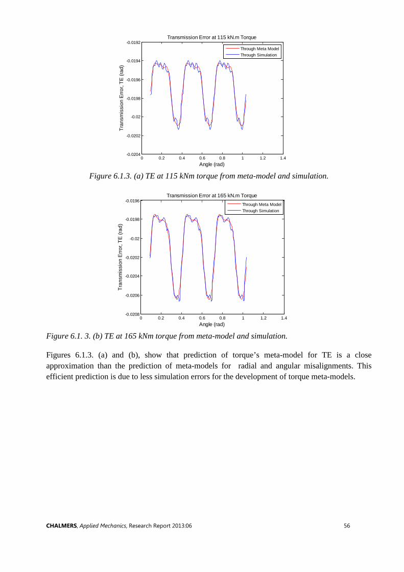
CHALMERS, Applied Mechanics, Research Report 2013:06 56
Figure 6.1.3. (a) TE at 115 kNm torque from meta-model and simulation.
Figure 6.1. 3. (b) TE at 165 kNm torque from meta-model and simulation.
Figures 6.1.3. (a) and (b), show that prediction of torque’s meta-model for TE is a close approximation than the prediction of meta-models for radial and angular misalignments. This efficient prediction is due to less simulation errors for the development of torque meta-models.
0 0.2 0.4 0.6 0.8 1 1.2 1.4-0.0204
-0.0202
-0.02
-0.0198
-0.0196
-0.0194
-0.0192
Angle (rad)
Tran
smis
sion
Erro
r, TE
(rad
)
Transmission Error at 115 kN.m Torque
Through Meta ModelThrough Simulation
0 0.2 0.4 0.6 0.8 1 1.2 1.4-0.0208
-0.0206
-0.0204
-0.0202
-0.02
-0.0198
-0.0196
Angle (rad)
Tran
smis
sion
Erro
r, TE
(rad
)
Transmission Error at 165 kN.m Torque
Through Meta ModelThrough Simulation
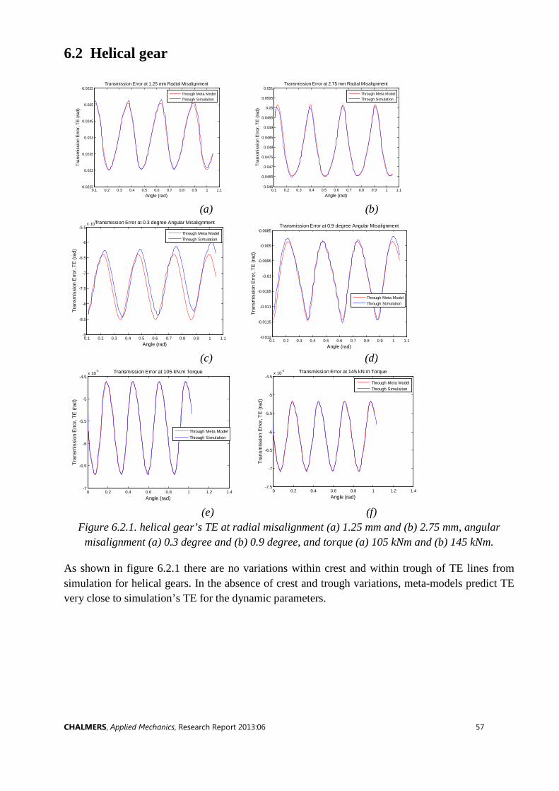
CHALMERS, Applied Mechanics, Research Report 2013:06 57
0.1 0.2 0.3 0.4 0.5 0.6 0.7 0.8 0.9 1 1.10.046
0.0465
0.047
0.0475
0.048
0.0485
0.049
0.0495
0.05
0.0505
0.051
Angle (rad)
Tran
smis
sion
Erro
r, TE
(rad
)
Transmission Error at 2.75 mm Radial Misalignment
Through Meta ModelThrough Simulation
0.1 0.2 0.3 0.4 0.5 0.6 0.7 0.8 0.9 1 1.1-0.012
-0.0115
-0.011
-0.0105
-0.01
-0.0095
-0.009
-0.0085
Angle (rad)
Tran
smis
sion
Erro
r, TE
(rad
)
Transmission Error at 0.9 degree Angular Misalignment
Through Meta ModelThrough Simulation
0 0.2 0.4 0.6 0.8 1 1.2 1.4-7.5
-7
-6.5
-6
-5.5
-5
-4.5x 10
-3
Angle (rad)
Tran
smis
sion
Erro
r, TE
(rad
)
Transmission Error at 145 kN.m Torque
Through Meta ModelThrough Simulation
6.2 Helical gear
(a) (b)
(c) (d)
(e) (f)
Figure 6.2.1. helical gear’s TE at radial misalignment (a) 1.25 mm and (b) 2.75 mm, angular misalignment (a) 0.3 degree and (b) 0.9 degree, and torque (a) 105 kNm and (b) 145 kNm.
As shown in figure 6.2.1 there are no variations within crest and within trough of TE lines from simulation for helical gears. In the absence of crest and trough variations, meta-models predict TE very close to simulation’s TE for the dynamic parameters.
0.1 0.2 0.3 0.4 0.5 0.6 0.7 0.8 0.9 1 1.10.0225
0.023
0.0235
0.024
0.0245
0.025
0.0255
Angle (rad)
Tran
smis
sion
Erro
r, TE
(rad
)Transmission Error at 1.25 mm Radial Misalignment
Through Meta ModelThrough Simulation
0.1 0.2 0.3 0.4 0.5 0.6 0.7 0.8 0.9 1 1.1-9
-8.5
-8
-7.5
-7
-6.5
-6
-5.5x 10
-3
Angle (rad)
Tran
smis
sion
Erro
r, TE
(rad
)
Transmission Error at 0.3 degree Angular Misalignment
Through Meta ModelThrough Simulation
0 0.2 0.4 0.6 0.8 1 1.2 1.4-7
-6.5
-6
-5.5
-5
-4.5x 10
-3
Angle (rad)
Tran
smis
sion
Erro
r, TE
(rad
)
Transmission Error at 105 kN.m Torque
Through Meta ModelThrough Simulation

CHALMERS, Applied Mechanics, Research Report 2013:06 58
0.1 0.2 0.3 0.4 0.5 0.6 0.7 0.8 0.9 1 1.10.0455
0.046
0.0465
0.047
0.0475
0.048
Angle (rad)
Tran
smis
sion
Erro
r, TE
(rad
)
Transmission Error at 1.75 mm Radial Misalignment
Through Meta ModelThrough Simulation
0.1 0.2 0.3 0.4 0.5 0.6 0.7 0.8 0.9 1 1.1-0.0285
-0.028
-0.0275
-0.027
-0.0265
-0.026
-0.0255
-0.025
Angle (rad)
Tran
smis
sion
Erro
r, TE
(rad
)
Transmission Error at 1.3 degree Angular Misalignment
Through Meta ModelThrough Simulation
0.1 0.2 0.3 0.4 0.5 0.6 0.7 0.8 0.9 1 1.10.0195
0.02
0.0205
0.021
0.0215
0.022
0.0225
0.023
0.0235
0.024
Angle (rad)
Tran
smis
sion
Erro
r, TE
(rad
)
Transmission Error at 155 kN.m Torque
Through Meta ModelThrough Simulation
6.3. Planetary gear
(a) (b)
(c) (d)
(e) (f)
Figure 6.3.1. planetary gear’s TE at radial misalignment (a) 0.25 mm and (b) 1.75 mm, angular misalignment (a) 0.1 degree and (b) 1.3 degree, and torque (a) 135 kNm and (b) 155 kNm.
In figure 6.3.1 meta-models predict TE very close to simulation’s TE for torque and angular misalignment but for radial misalignment the prediction is not so close to the local peak values. By improving matlab coding to capture sinusoidal form at the local peak values, this kind of misfit can be minimized.
Evaluation for combined meta-models for radial misalignment, angular misalignment and torque cannot be done without considering the dependent dynamic parameters, because for the project work the dynamic parameters are considered independent.
0.1 0.2 0.3 0.4 0.5 0.6 0.7 0.8 0.9 1 1.10.022
0.023
0.024
0.025
0.026
0.027
0.028
Angle (rad)
Tran
smis
sion
Erro
r, TE
(rad
)
Transmission Error at 0.25 mm Radial Misalignment
Through Meta ModelThrough Simulation
0.1 0.2 0.3 0.4 0.5 0.6 0.7 0.8 0.9 1 1.1-0.024
-0.023
-0.022
-0.021
-0.02
-0.019
-0.018
Angle (rad)
Tran
smis
sion
Erro
r, TE
(rad
)
Transmission Error at 0.1 degree Angular Misalignment
Through Meta ModelThrough Simulation
0.1 0.2 0.3 0.4 0.5 0.6 0.7 0.8 0.9 1 1.10.0195
0.02
0.0205
0.021
0.0215
0.022
0.0225
0.023
0.0235
0.024
Angle (rad)
Tran
smis
sion
Erro
r, TE
(rad
)
Transmission Error at 135 kN.m Torque
Through Meta ModelThrough Simulation

CHALMERS, Applied Mechanics, Research Report 2013:06 59
7 Conclusion
It is concluded from the project work that calculating TE from meta-models can be a computationally attainable method compared to calculating the TE from complex FE-models of the gear geometry.
The meta-models developed here represent the TE by a four terms sinusoidal form wherein each coefficient is described by 4th order of polynomial of the input parameter. Meta-models for the dynamic parameters (radial and angular misalignments and torque) are developed at particular values of static parameters (gear ratio, pressure angle, and addendum). Those developed meta-models will not be valid anymore for different values of the static parameters.
Lack of fit of the meta-model is because of some reasons. One of the likely reasons is the simulation errors, and adjusting the “phase” due to different starting positions. Accuracy of meta-model can be increased by minimizing the simulation errors. Because of the nature of used sinusoidal form, meta-model cannot predict variations within the crest and within the trough of TE. Combined meta-model cannot predict TE accurately because of considering the independent dynamic parameters.
Meta-models predictions of TE for the dynamic parameters are more reliable than predictions of TE for the static parameters.

CHALMERS, Applied Mechanics, Research Report 2013:06 60
8 Future work
Still engineers are struggling to find out the simple and easy solutions to the engineering problems in different real life applications. The methodology which is used for the project work can provide simple, easy and reliable solutions to the engineering problems.
In case of the same working area of this project, it might be of interest for real life applications to develop a meta-model of the dependent dynamic parameters. The meta-modeling technique can also be applied to determine the contact and reaction forces of gears. In the static parameters of the project work, other important parameters like tip relief can also be included. Before applying the results of scientific research, it is a demand to validate the results against experiments. An interesting possibility would be to use a test rig, currently being developed at the division of Dynamics, Chalmers University of Technology [27], at which the reaction forces and transmission error can be measured in a simple gear system.

CHALMERS, Applied Mechanics, Research Report 2013:06 61
References
[1] The AWEA U.S. Wind Industry, "Industry Statistics," American Wind Energy Association, 04 September, 2013. [Online]. Available: http://www.awea.org/learnabout/industry_stats/.
[2] An agency of the United States government, "Advanced wind turbine drive train Concept: Workshop report," U.S. Department of Energy: Wind and water power program, 29-30 June 2010. [Online]. Available: http://www.nrel.gov/docs/fy11osti/50043.pdf.
[3] Puigcorbe and De-Beaumont, "Wind Turbine Gearbox Reliability," Renewable energy world.com, 26 May 2013. [Online]. Available: http://www.renewableenergyworld.com/rea/news/article/2010/06/wind-turbine-gearbox-reliability.
[4] Adam M. Ragheb and Magdi Ragheb, "Wind Turbine Gearbox Technologies," Department of Aerospace Engineering,Department of Nuclear, Plasma and Radiological Engineering,University of Illinois at Urbana-Champaign, 216 Talbot Laboratory, USA, 2011.
[5] Gu and Velex, "On the dynamic simulation of eccentricity errors in planetary gears," Mechanism and Machine Theory, vol. 61, pp. 14-29, 2013.
[6] Guo, Robert and Parker, "Dynamic modeling and analysis of a spur planetary gear involving tooth wedging and bearing clearance nonlinearity," European Journal of Mechanics A/Solids, vol. 29, no. 6, pp. 1022-1033, 2010.
[7] Khabou, Bouchaala, Fakhfakh and Haddar, "Study of a spur dynamic behavior in transient regime," Mechanical Systems and Signal Processing, vol. 25, no. 8, pp. 3089-3101, 2011.
[8] Sankar and Nataraj, "Prevention of helical gear tooth damage in wind turbine generator: a case study," Proceedings of the Institution of Mechanical Engineers, Part A: Journal of Power and Energy, vol. 224, no. 8 , pp. 1117-1125, December 2010.
[9] Michaelis, Hölm and Hinterstoiber, "Influence factors on gearbox power loss," Industrial Lubrication and Tribology, vol. 63, no. 1, pp. 46-55, July 20-24, 2009.
[10] Ambarisha and Parker, "Nonlinear dynamics of planetary gears using analytical and finite element models," Journal of Sound and Vibration, vol. 302, no. 3, pp. 577-595, 2007.
[11] Abboudi, Walha, Driss, Fakhfakh and Mohamed, "Dynamic behavior of a two-stage gear train used in a fixed-speed wind turbine," Mechanism and Machine Theory, vol. 46, no. 12, pp. 1888-1900, 2011.
[12] Karpat, Ekwaro-Osire, Cavdar and Babalik, "Dynamic analysis of involute spur gears with asymmetric teeth," International Journal of Mechanical Sciences, vol. 50, no. 12, pp. 1598-1610, 2008.

CHALMERS, Applied Mechanics, Research Report 2013:06 62
[13] Barszcz and Randall, "Application of spectral kurtosis for detection of a tooth crack in the planetary gear of a wind turbine," Mechanical Systems and Signal Processing, vol. 23, no. 4, pp. 1352-1365, 2009.
[14] Pedersen, Santos and Hede, "Advantages and drawbacks of applying periodic time-variant modal analysis to spur gear dynamics," Mechanical Systems and Signal Processing, vol. 24, no. 5, pp. 1495-1508, 2010.
[15] R. Tharmakulasingam, "Transmission Error in Spur Gears: Static and Dynamic," Brunel University United Kingdom, October 2009.
[16] Gu and Velex, "A dynamic model to study the influence of planet position errors in planetary gears," Journal of Sound and Vibration, vol. 331, no. 20, pp. 4554-4574, 2012.
[17] R. G. Munro, "A review of the theory and measurement of gear transmission error," Proceedings of the First IMechE Conference on Gearbox Noise and Vibration, pp. 3-10, 1990.
[18] Adam Ragheb and Magdi Ragheb, "Technologies, Wind Turbine Gearbox," in Proceedings of the 1st International Nuclear and Renewable Energy Conference (INREC10), Urbana, Illinois 61801, USA., March 21-24, 2010.
[19] Crowther, Ramakrishnan, Zaidi and Halse, "Sources of time varying contact stress and misalignments in wind turbine planetary sets," Wind Energy, vol. 14, no. 5, pp. 637-651, 2011.
[20] Karimpour, Dearn and Walton, "A kinematic analysis of meshing polymer gear teeth," Journal of Materials Design and Applications, vol. 224, no. 3, pp. 101-115, Jul 2010.
[21] K. Mao, "An approach for powertrain gear transmission error prediction using the non-linear finite element method," Journal of Automobile Engineering, vol. 220, no. 10, pp. 1454-1463, Oct 2006.
[22] Andrade and Prashant, "Simulation of a Parking Pawl Mechanism with Abaqus/Standard and Abaqus/Explicit," in Ford Motor Company Hibbitt, Karlsson & Sorensen (Michigan), Inc., 2002.
[23] Howard and Wang, "The torsional stiffness of involute spur gears," Journal of Mechanical Engineering Science, vol. 218, no. 1, pp. 131-142, January 1, 2004.
[24] Li, Chiou, Hung, Chang and Yen, "Integration of finite element analysis and optimum design on gear systems," Finite Elements in Analysis and Design, vol. 38, no. 3, pp. 179-192, 2002.
[25] Sommer and Patrick, "Vibration-based health monitoring of multiple -stage gear train and differential planetary transmission involving teeth damage and backlashnonlinearity," San Luis Obispo, 2011.
[26] R. Xu, "Finite element modelling and simulation on the quenching effectfor spur gear design optimization," The Graduate Faculty of the University of Akron, Akron, August, 2008.
[27] M. S. Gabriel, "Design of Experiments and Analysis for Drive Train Test Rig," Master’s thesis 2013:30, ISSN 1652-8557, Department of Applied Mechanics, Division of Dynamics, Chalmers University of

CHALMERS, Applied Mechanics, Research Report 2013:06 63
Technology, Göteborg, 2013.
[28] Villa, Renones, Peran and Miguel, "Statistical fault diagnosis based on vibration analysis for gear test-bench under non-stationary conditions of speed and load," Mechanical Systems and Signal Processing, vol. 29, pp. 436-446, 2012.
[29] G. E. Brown, "nees@oklahoma," Systèmes, Dassault, [Online]. Available: http://www.nees.ou.edu/abaqus.html.
[30] Zhu, Xu, Lim, Du and Liu, "Effect of flexible pin on the dynamic behaviours of wind turbine planetary gear drives," Journal of Mechanical Engineering Science, vol. 227, no. 1, pp. 74-86, Dec 17, 2012.
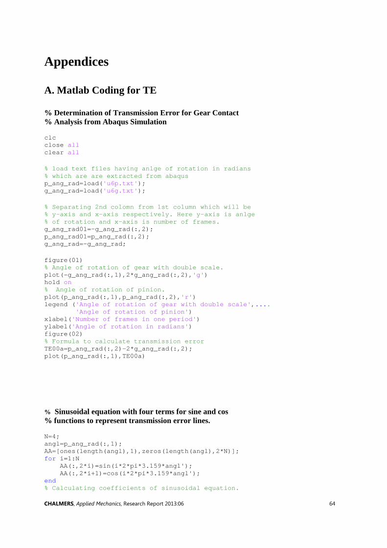
CHALMERS, Applied Mechanics, Research Report 2013:06 64
Appendices
A. Matlab Coding for TE
% Determination of Transmission Error for Gear Contact % Analysis from Abaqus Simulation
clc close all clear all % load text files having anlge of rotation in radians % which are are extracted from abaqus p_ang_rad=load('u6p.txt'); g_ang_rad=load('u6g.txt'); % Separating 2nd colomn from 1st column which will be % y-axis and x-axis respectively. Here y-axis is anlge % of rotation and x-axis is number of frames. g_ang_rad01=-g_ang_rad(:,2); p_ang_rad01=p_ang_rad(:,2); g_ang_rad=-g_ang_rad; figure(01) % Angle of rotation of gear with double scale. plot(-g_ang_rad(:,1),2*g_ang_rad(:,2),'g') hold on % Angle of rotation of pinion. plot(p_ang_rad(:,1),p_ang_rad(:,2),'r') legend ('Angle of rotation of gear with double scale',.... 'Angle of rotation of pinion') xlabel('Number of frames in one period') ylabel('Angle of rotation in radians') figure(02) % Formula to calculate transmission error TE00a=p_ang_rad(:,2)-2*g_ang_rad(:,2); plot(p_ang_rad(:,1),TE00a) % Sinusoidal equation with four terms for sine and cos % functions to represent transmission error lines.
N=4; angl=p_ang_rad(:,1); AA=[ones(length(angl),1),zeros(length(angl),2*N)]; for i=1:N AA(:,2*i)=sin(i*2*pi*3.159*angl'); AA(:,2*i+1)=cos(i*2*pi*3.159*angl'); end % Calculating coefficients of sinusoidal equation.
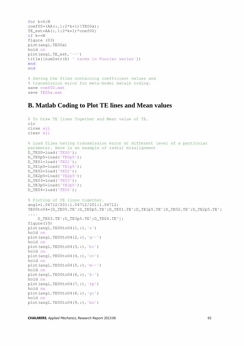
CHALMERS, Applied Mechanics, Research Report 2013:06 65
for k=0:N coef00=(AA(:,1:2*k+1)\TE00a); TE_est=AA(:,1:2*k+1)*coef00; if k==N figure (03) plot(angl,TE00a) hold on plot(angl,TE_est,'--') title([num2str(k) ' terms in Fourier series']) end end % Saving the files containing coefficient values and % transmission error for meta-model matalb coding. save coef00.mat save TE00a.mat
B. Matlab Coding to Plot TE lines and Mean values
% To Draw TE lines Together and Mean value of TE. clc close all clear all % Load files having transmission error at different level of a particular parameter. Here is an example of radial misalignment D_TE00=load('TE00'); D_TE0p5=load('TE0p5'); D_TE01=load('TE01'); D_TE1p5=load('TE1p5'); D_TE02=load('TE02'); D_TE2p5=load('TE2p5'); D_TE03=load('TE03'); D_TE3p5=load('TE3p5'); D_TE04=load('TE04'); % Ploting of TE lines together. angl=1.04712/201:1.04712/201:1.04712; TE00to04=[D_TE00.TE';D_TE0p5.TE';D_TE01.TE';D_TE1p5.TE';D_TE02.TE';D_TE2p5.TE';.... D_TE03.TE';D_TE3p5.TE';D_TE04.TE']; figure(10) plot(angl,TE00to04(1,:),'r') hold on plot(angl,TE00to04(2,:),'g--') hold on plot(angl,TE00to04(3,:),'b:') hold on plot(angl,TE00to04(4,:),'c+') hold on plot(angl,TE00to04(5,:),'m--') hold on plot(angl,TE00to04(6,:),'k-') hold on plot(angl,TE00to04(7,:),'rp') hold on plot(angl,TE00to04(8,:),'g:') hold on plot(angl,TE00to04(9,:),'bo')

CHALMERS, Applied Mechanics, Research Report 2013:06 66
xlabel('Angle (rad)','FontSize',12) ylabel('Transmission Error, TE (rad)','FontSize',12) title('Transmission Error Vs Radial Misalignment (mm)','FontSize',12) legend('TE04','TE3.5','TE03','TE2.5','TE02','TE1.5','TE01','TE0.5','TE00','Location','SouthEast') % Calculatin mean values for each TE line. mTE1=mean(TE00to04(1,1:end)); mTE2=mean(TE00to04(2,1:end)); mTE3=mean(TE00to04(3,1:end)); mTE4=mean(TE00to04(4,1:end)); mTE5=mean(TE00to04(5,1:end)); mTE6=mean(TE00to04(6,1:end)); mTE7=mean(TE00to04(7,1:end)); mTE8=mean(TE00to04(8,1:end)); mTE9=mean(TE00to04(9,1:end)); mTE=[mTE1 mTE2 mTE3 mTE4 mTE5 mTE6 mTE7 mTE8 mTE9]; figure(11) plot (0:0.5:4,mTE,'-*') xlabel('Radial Misalignment (mm)','FontSize',12) ylabel(' Mean of Transmission Error, TE (rad)','FontSize',12) title('Mean of Transmission Error Vs Radial Misalignment (mm)','FontSize',12)
C. Matlab Coding for Meta-model and Polynomial Fit of Coefficients % Meta-model and Polynomial Fit of Coefficients of Sinusoidal Equation. clc close all clear % Load files having vlaues for coefficients at particular level of TE. % Here is an example for radial misalignment. load coef00 load coef0p5 load coef01 load coef1p5 load coef02 load coef2p5 load coef03 load coef3p5 load coef04 % Values for radial misalignment ma=[0:0.5:04]; ma=ma'; coeffmat=[coef00,coef0p5,coef01,coef1p5,coef02,coef2p5,coef03,coef3p5,coef04]; % Values for each coefficient at different level of TE. a0=coeffmat(1,:); a1=coeffmat(2,:); b1=coeffmat(3,:); a2=coeffmat(4,:); b2=coeffmat(5,:); a3=coeffmat(6,:); b3=coeffmat(7,:); a4=coeffmat(8,:); b4=coeffmat(9,:); % Polynomial fit for coefficients. fa0 = fit(ma, a0', 'poly4'); coefa0=coeffvalues(fa0); fa1 = fit(ma, a1', 'poly4'); coefa1=coeffvalues(fa1);

CHALMERS, Applied Mechanics, Research Report 2013:06 67
fa2 = fit(ma, a2', 'poly4'); coefa2=coeffvalues(fa2); fa3 = fit(ma, a3', 'poly4'); coefa3=coeffvalues(fa3); fa4 = fit(ma, a4', 'poly4'); coefa4=coeffvalues(fa4); fb1 = fit(ma, b1', 'poly4'); coefb1=coeffvalues(fb1); fb2 = fit(ma, b2', 'poly4'); coefb2=coeffvalues(fb2); fb3 = fit(ma, b3', 'poly4'); coefb3=coeffvalues(fb3); fb4 = fit(ma, b4', 'poly4'); coefb4=coeffvalues(fb4); coeffmat_est=[coefa0;coefa1;coefb1;coefa2;coefb2;coefa3;coefb3;coefa4;coefb4]; % Ploting meta-model TE and simulation TE together. shb01=input('Enter radial misalignment till 04 millimeter by increment of 0.5 millimeter'); shb=[shb01^4 shb01^3 shb01^2 shb01 1]; coeffmat_est01=zeros(9,1); for ci=1:9 coeffmat_est01(ci,1)=coeffmat_est(ci,:)*shb'; end N=4; AA=[ones(length(angl),1),zeros(length(angl),2*N)]; for i=1:N AA(:,2*i)=sin(i*2*pi*3.159*angl'); AA(:,2*i+1)=cos(i*2*pi*3.159*angl'); end TE_est=AA*coeffmat_est01; figure (01) plot (angl,TE_est,'r') hold on if shb01==0 plot (TE00a) elseif shb01==0.5 plot (TE0p5a) elseif shb01==01 plot (TE01a) elseif shb01==1.5 plot (TE1p5a) elseif shb01==02 plot (TE02a) elseif shb01==2.5 plot (TE2p5a) elseif shb01==03 plot (TE03a) elseif shb01==3.5 plot (TE3p5a) elseif shb01==04 plot (angl,TE04a) end legend ('Through Meta Model','Through Simulation') xlabel('Angle (rad)','FontSize',12) ylabel('Transmission Error, TE (rad)','FontSize',12) title('Transmission Error 04 mm Radial Misalignment','FontSize',12) % Ploting coefficients coefficients=[a0',a1', a2', a3', a4', b1', b2', b3', b4']; figure (30)

CHALMERS, Applied Mechanics, Research Report 2013:06 68
plot (coefficients) legend('a0','a1','a2','a3','a4','b1','b2','b3','b4') xlabel('Radial Misalignment (mm)','FontSize',12) ylabel('coefficients values','FontSize',12) title('Coefficients','FontSize',12)
D. Matlab Coding for Radial and Angular Misalignments Meta-models % Radial and Angular Misalignments Meta-models. clc close all clear all % Load file at radial misalignment 00mm and angular misalignment from 0 % degree to 2 degree. load TEm0s0to2 % Load file at radial misalignment 01mm and angular misalignment from 0 % degree to 2 degree. load TEm1s0to2 % Load file at radial misalignment 02mm and angular misalignment from 0 % degree to 2 degree. load TEm2s0to2 % Load file at radial misalignment 03mm and angular misalignment from 0 % degree to 2 degree. load TEm3s0to2 % Load file at radial misalignment 04mm and angular misalignment from 0 % degree to 2 degree. load TEm4s0to2 angl=0:0.03/60:0.03; TEm0to4s0to2=[TEm0s0to2,TEm1s0to2,TEm2s0to2,TEm3s0to2,TEm4s0to2]; figure(10) plot(angl,TEm0to4s0to2) xlabel('Angle (rad)') ylabel('Transmission Error, TE (rad)') title('Transmission Error Vs Radial and Angular Misalignment','FontSize',12) % Ploting all TE lines figure(8) subplot (2,2,1) plot(angl,TEm0to4s0to2(1:61,6),'r') hold on plot(angl,TEm0to4s0to2(1:61,7),'g--') hold on plot(angl,TEm0to4s0to2(1:61,8),'b:') hold on plot(angl,TEm0to4s0to2(1:61,9),'c+') hold on plot(angl,TEm0to4s0to2(1:61,10),'m-.') legend('TE-A00','TE-A0.5','TE-A01','TE-A1.5','TE-A02','FontSize',12) ylabel('Transmission Error, TE (rad)') title('Misalignment: Radial 01mm, Angular 0 to 2 degree','FontSize',12) subplot (2,2,2) plot(angl,TEm0to4s0to2(1:61,11),'r') hold on plot(angl,TEm0to4s0to2(1:61,12),'g--') hold on plot(angl,TEm0to4s0to2(1:61,13),'b:') hold on

CHALMERS, Applied Mechanics, Research Report 2013:06 69
plot(angl,TEm0to4s0to2(1:61,14),'c+') hold on plot(angl,TEm0to4s0to2(1:61,15),'m-.') legend('TE-A00','TE-A0.5','TE-A01','TE-A1.5','TE-A02','FontSize',12) title('Misalignment: Radial 02mm, Angular 0 to 2 degree','FontSize',12) subplot (2,2,3) plot(angl,TEm0to4s0to2(1:61,16),'r') hold on plot(angl,TEm0to4s0to2(1:61,17),'g--') hold on plot(angl,TEm0to4s0to2(1:61,18),'b:') hold on plot(angl,TEm0to4s0to2(1:61,19),'c+') hold on plot(angl,TEm0to4s0to2(1:61,20),'m-.') legend('TE-A00','TE-A0.5','TE-A01','TE-A1.5','TE-A02','FontSize',12) xlabel('Angle (rad)') ylabel('Transmission Error, TE (rad)') title('Misalignment: Radial 03mm, Angular 0 to 2 degree','FontSize',12) subplot (2,2,4) plot(angl,TEm0to4s0to2(1:61,21),'r') hold on plot(angl,TEm0to4s0to2(1:61,22),'g--') hold on plot(angl,TEm0to4s0to2(1:61,23),'b:') hold on plot(angl,TEm0to4s0to2(1:61,24),'c+') hold on plot(angl,TEm0to4s0to2(1:61,25),'m-.') legend('TE-A00','TE-A0.5','TE-A01','TE-A1.5','TE-A02','FontSize',12) xlabel('Angle (rad)') title('Misalignment: Radial 04mm, Angular 0 to 2 degree','FontSize',12)
E. Meshing Technique
Seed Number 2D View
Seed Number 2D View
01
05
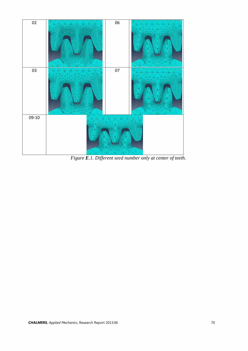
CHALMERS, Applied Mechanics, Research Report 2013:06 70
02
06
03
07
09-10
Figure E.1. Different seed number only at center of teeth.


![[1] involuteΣiii(spur and helical gear design system)Spur...1 [1] involuteΣiii(spur and helical gear design system) 図1.1 involuteΣiii(spur and helical) 1.1 概要 involuteΣⅲ(spur](https://img.pdfslide.net/doc/110x75/5ae0683d7f8b9a97518d2bd7/1-involuteiiispur-and-helical-gear-design-system-spur1-1-involuteiiispur.jpg)