Metagenomics & metagenomic assembly ... - DTU … · Center for Biological Sequence Analysis ... Simon Rasmussen 36626: Next Generation Sequencing analysis DTU Bioinformatics. 36626

36626 - Next Generation Sequencing Analysis

Preprocessing and SNP calling Natasja S. Ehlers, PhD student Center for Biological Sequence Analysis Functional Human Variation Group

Metagenomics & metagenomic assembly

Simon Rasmussen36626: Next Generation Sequencing analysis

DTU Bioinformatics


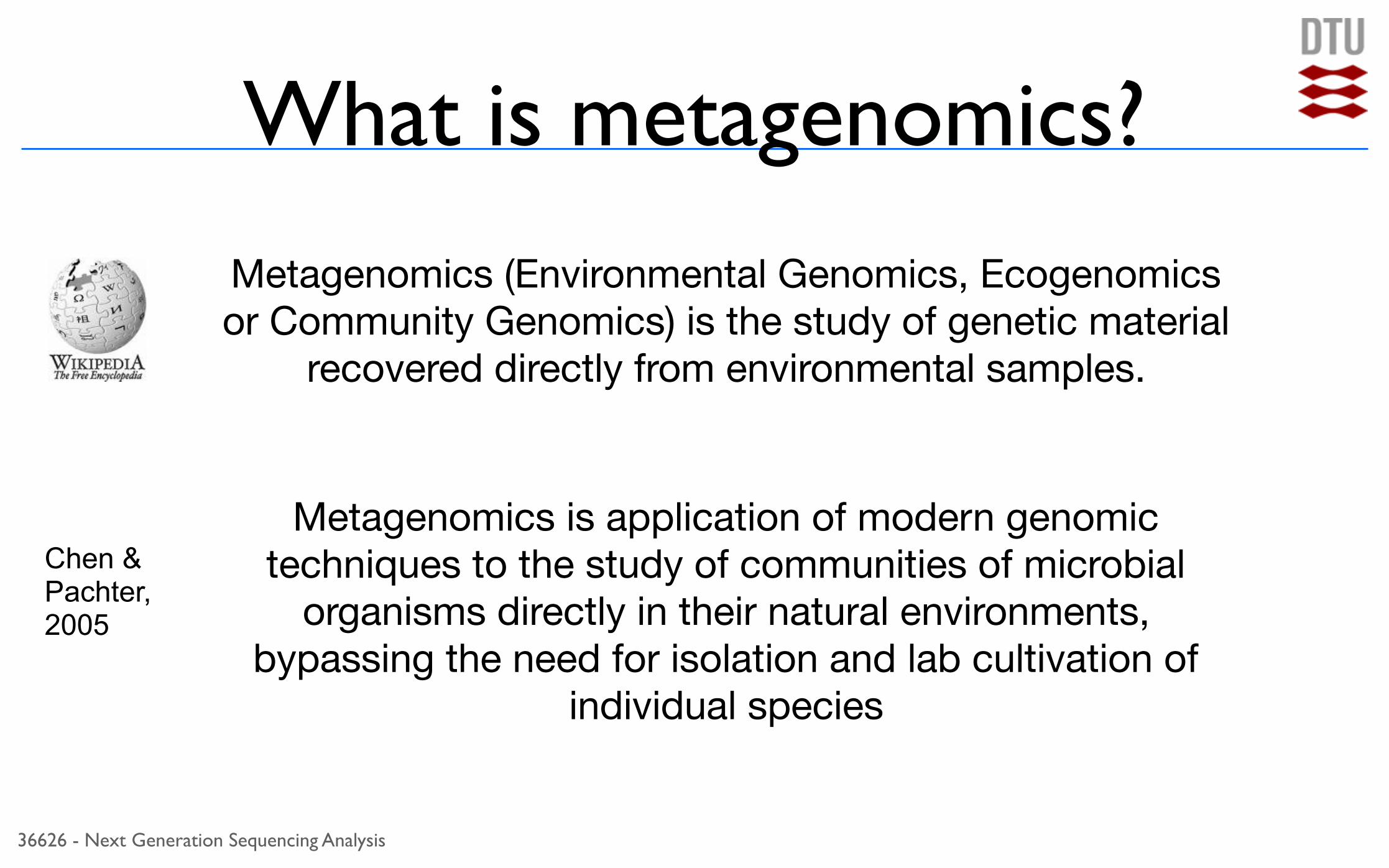
What is metagenomics?

Metagenomics (Environmental Genomics, Ecogenomics or Community Genomics) is the study of genetic material

recovered directly from environmental samples.

Metagenomics is application of modern genomic techniques to the study of communities of microbial

organisms directly in their natural environments, bypassing the need for isolation and lab cultivation of

individual species

Chen &Pachter,2005


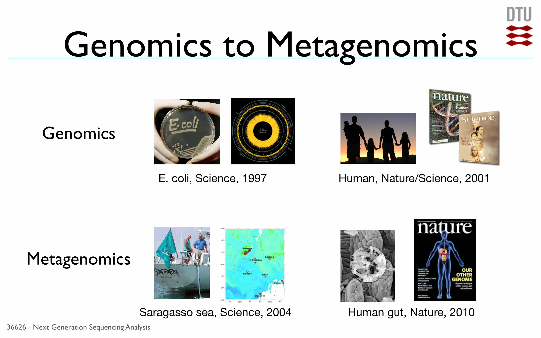
Genomics to Metagenomics

Genomics

Metagenomics

E. coli, Science, 1997 Human, Nature/Science, 2001

Saragasso sea, Science, 2004 Human gut, Nature, 2010


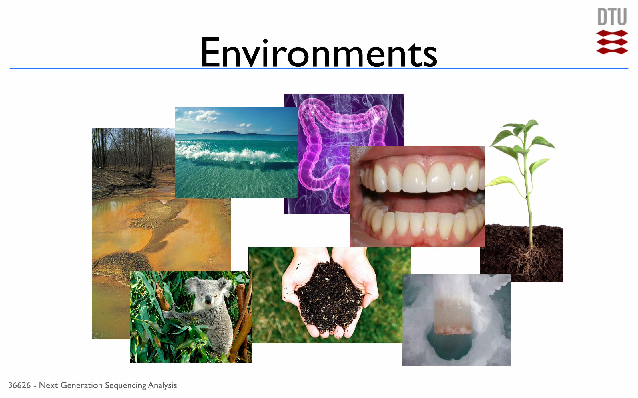
Environments


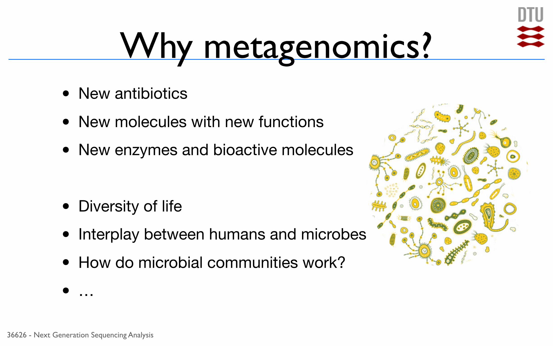
Why metagenomics?• New antibiotics

• New molecules with new functions

• New enzymes and bioactive molecules

• Diversity of life

• Interplay between humans and microbes

• How do microbial communities work?

• …


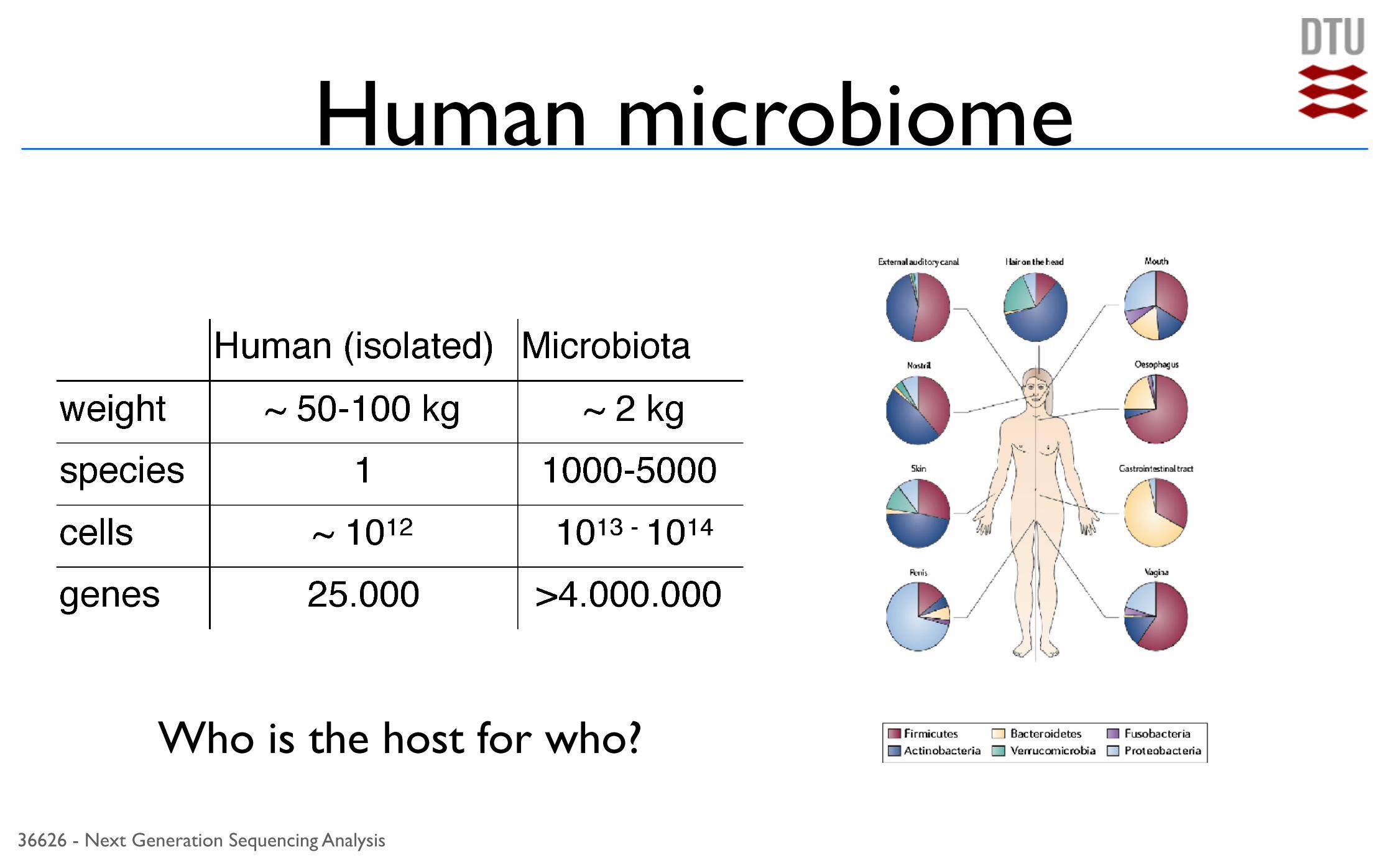
Human microbiome

Who is the host for who?


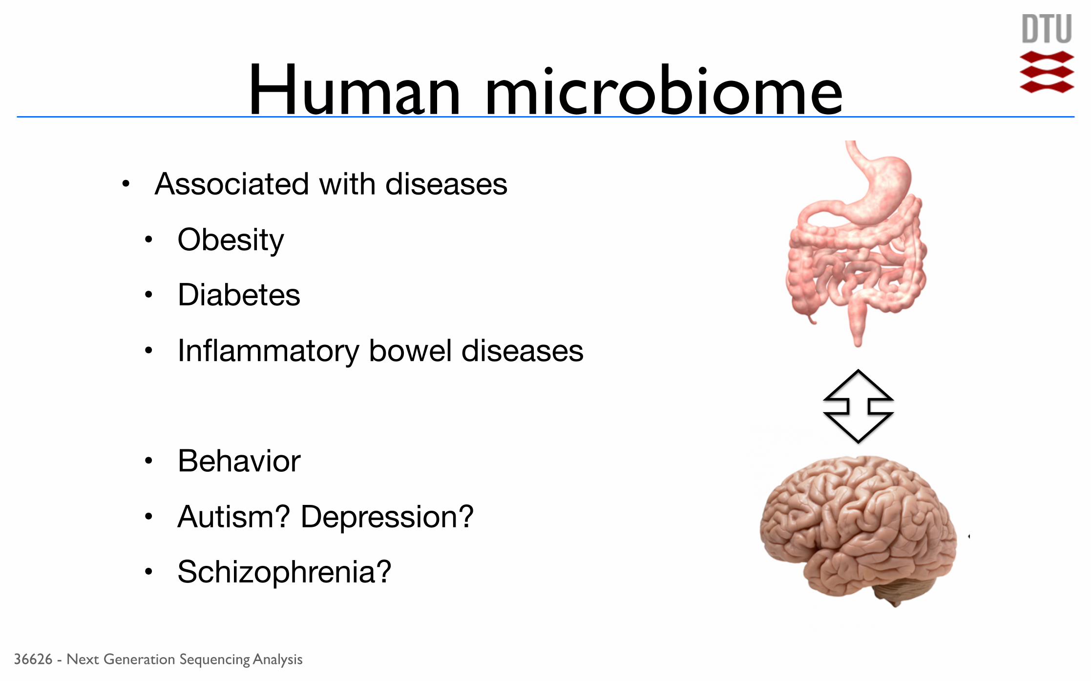
Human microbiome• Associated with diseases

• Obesity• Diabetes

• Inflammatory bowel diseases

• Behavior

• Autism? Depression?• Schizophrenia?


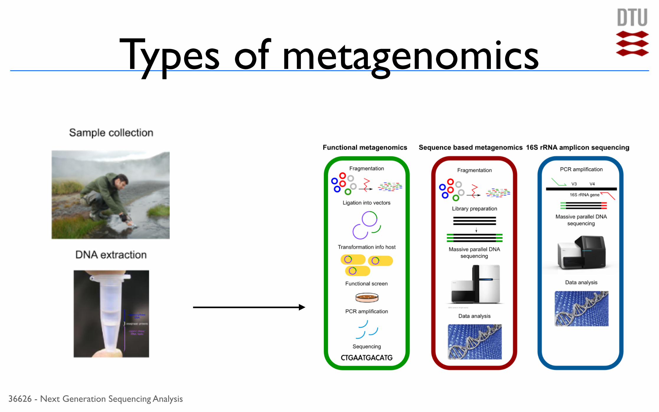
Types of metagenomicsHow to?How to?


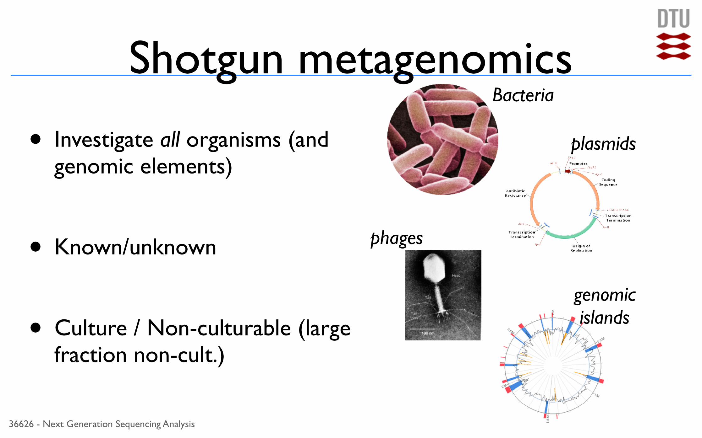
Shotgun metagenomics

• Investigate all organisms (and genomic elements)

• Known/unknown

• Culture / Non-culturable (large fraction non-cult.)

Bacteria

plasmids

phages

genomicislands

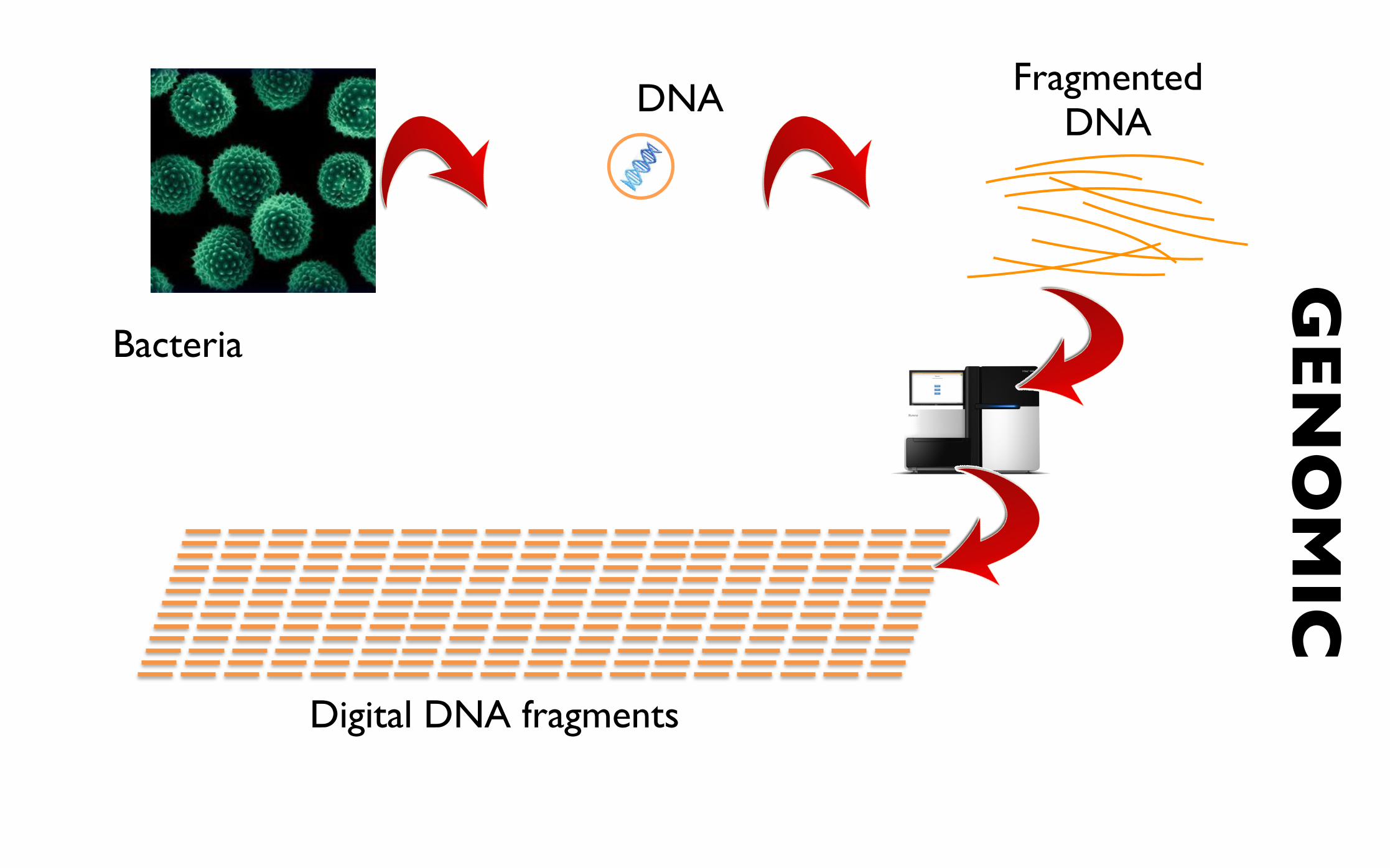
Bacteria

Fragmented DNA

Digital DNA fragments

GEN

OM

ICDNA

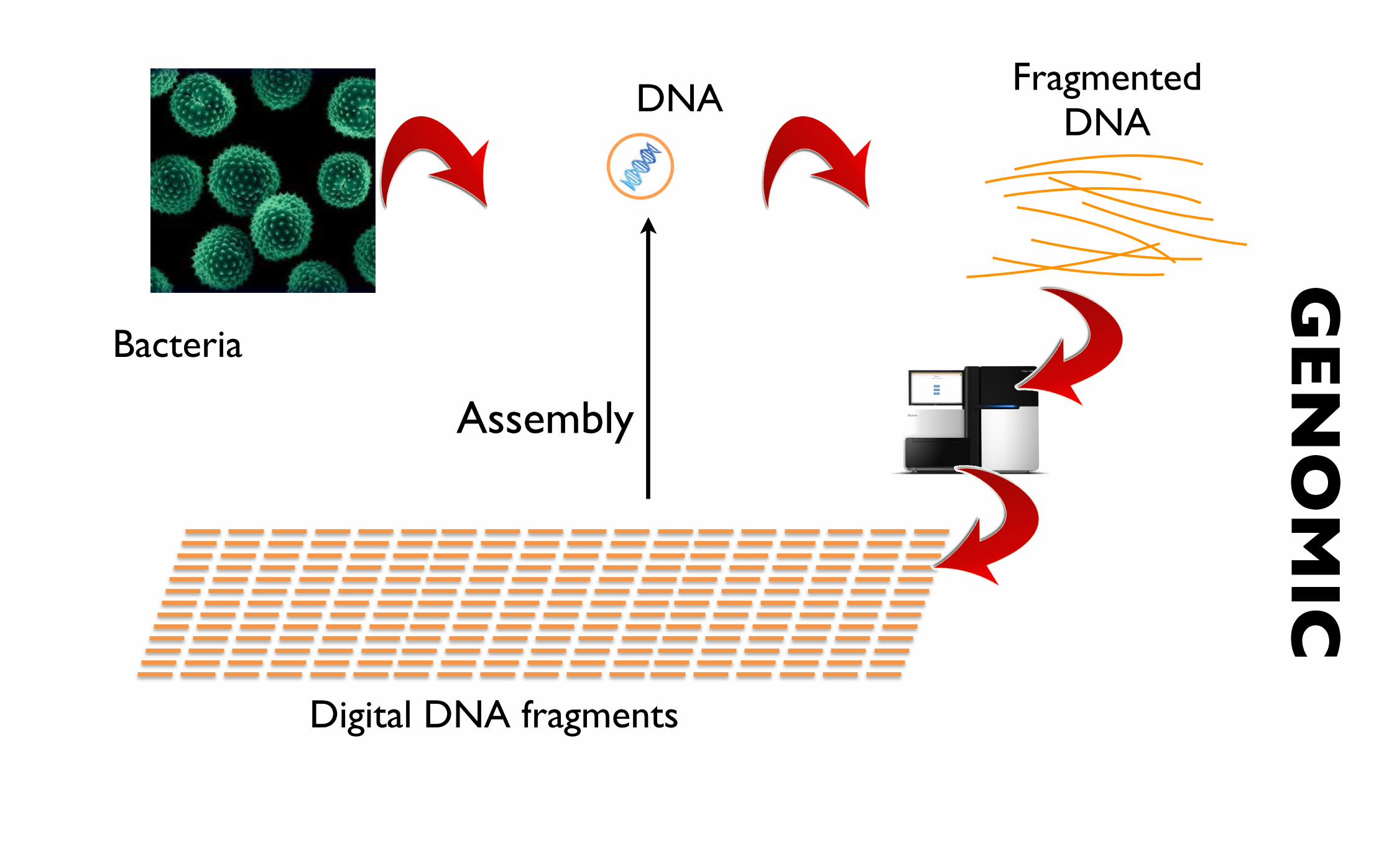
Bacteria

Fragmented DNA

Digital DNA fragments

GEN

OM

ICDNA

Assembly

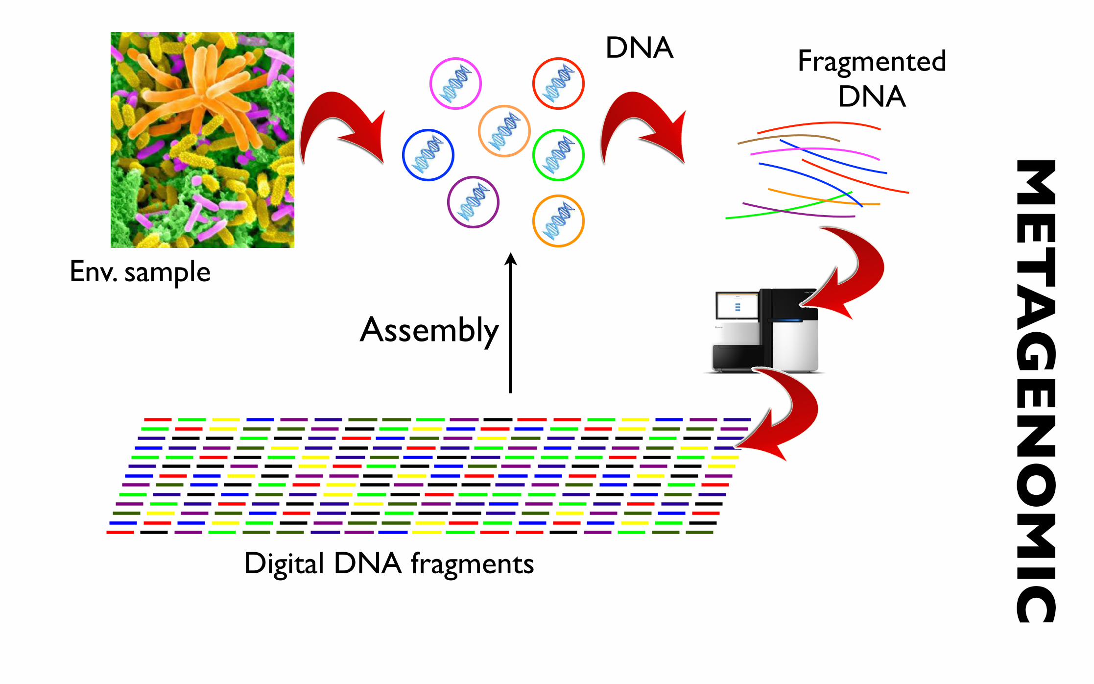
Env. sample

DNA Fragmented DNA

Digital DNA fragments Digital DNA fragments

MET

AG

ENO

MIC

Assembly

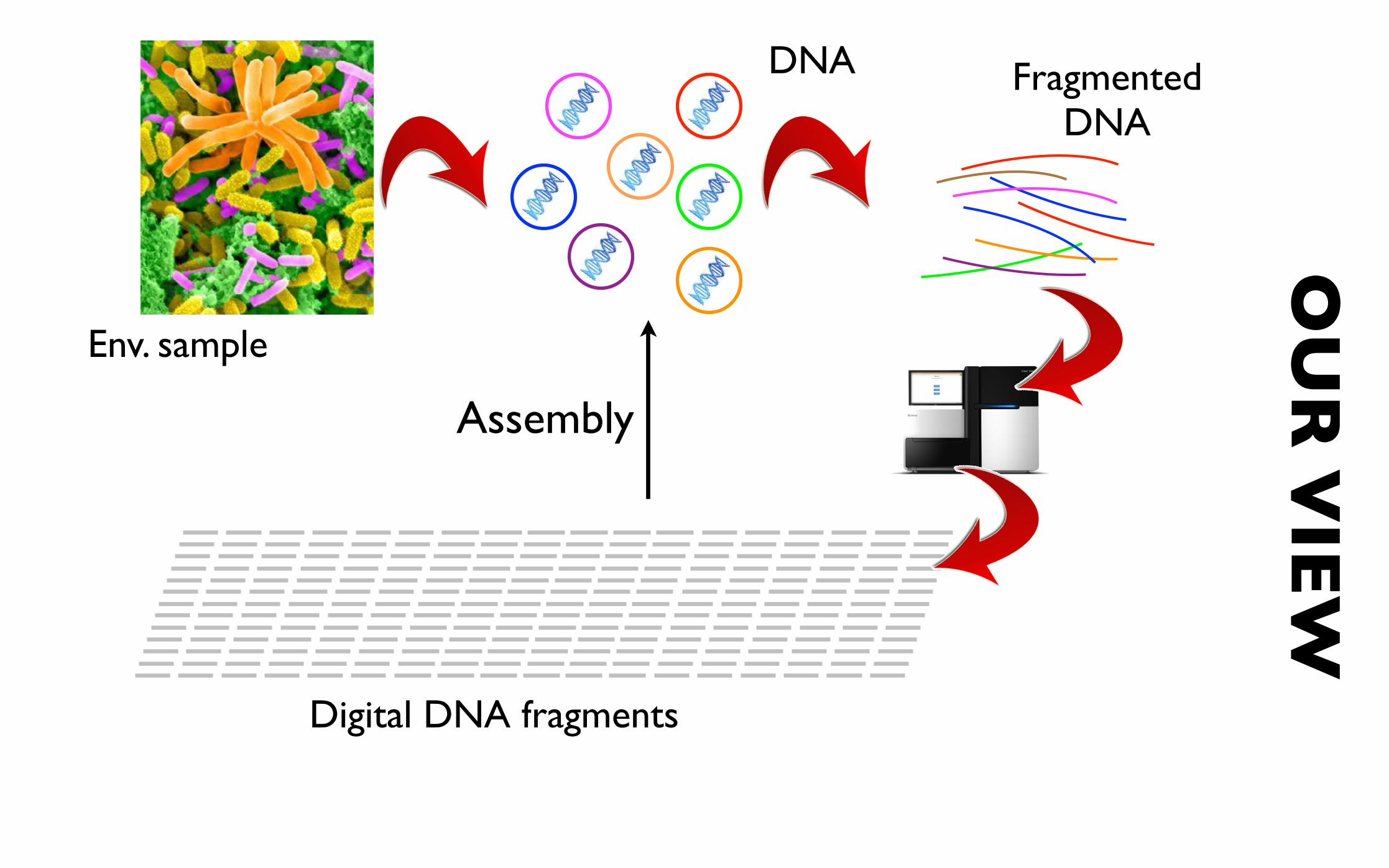
Env. sample

Fragmented DNA

OU

R V

IEW

Digital DNA fragments Digital DNA fragments

DNA

Assembly


Metagenomic assembly ...is even harder than single genome assembly


Why?

Can you think of why?

Groups of 2-3 3 mins


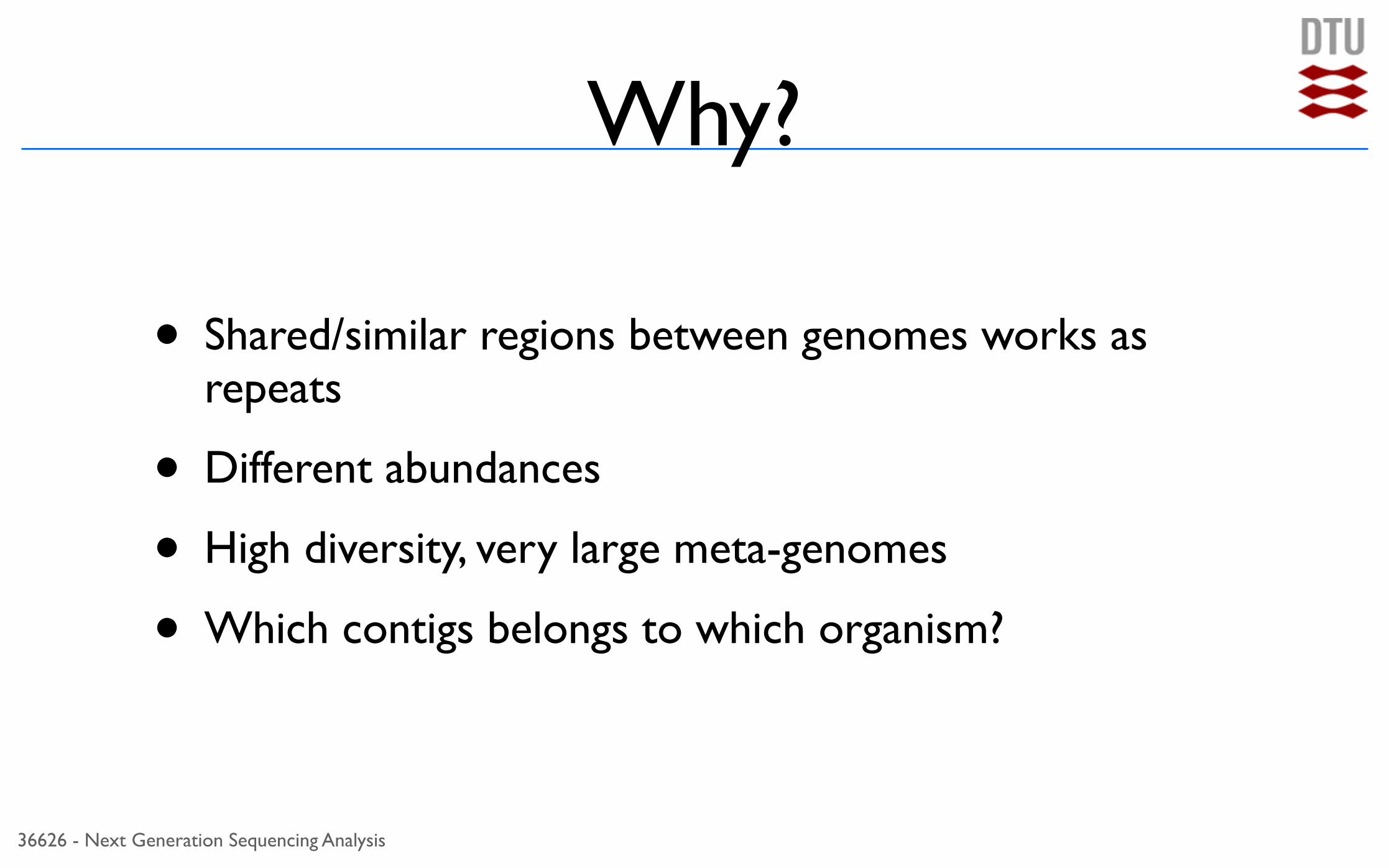
Why?

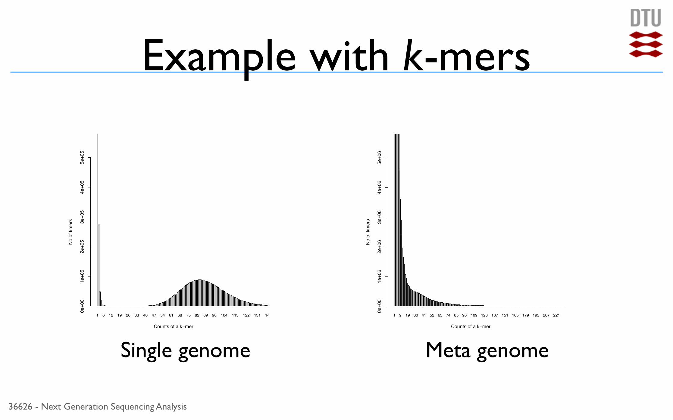
• Shared/similar regions between genomes works as repeats

• Different abundances

• High diversity, very large meta-genomes

• Which contigs belongs to which organism?


Example with k-mers

1 9 19 30 41 52 63 74 85 96 109 123 137 151 165 179 193 207 221

Counts of a k−mer

No

of k

mer

s

0e+0

01e

+06

2e+0

63e

+06

4e+0

65e

+06

1 6 12 19 26 33 40 47 54 61 68 75 82 89 96 104 113 122 131 140

Counts of a k−mer

No

of k

mer

s

0e+0

01e

+05

2e+0

53e

+05

4e+0

55e

+05

Single genome Meta genome


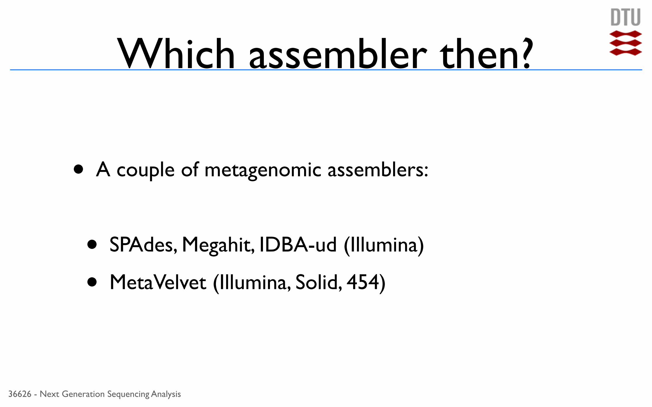
Which assembler then?

• A couple of metagenomic assemblers:

• SPAdes, Megahit, IDBA-ud (Illumina)

• MetaVelvet (Illumina, Solid, 454)


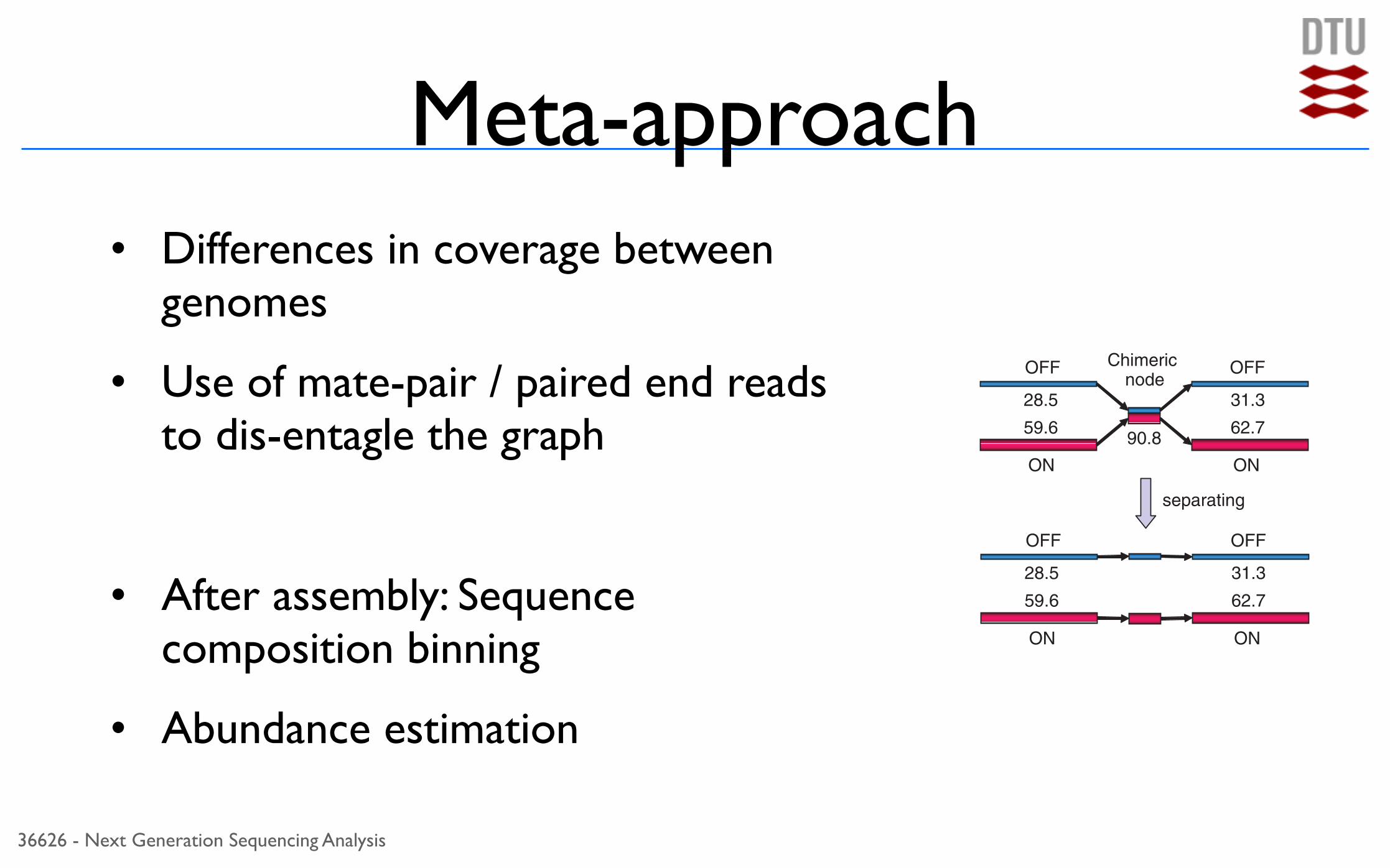
Meta-approach• Differences in coverage between

genomes

• Use of mate-pair / paired end reads to dis-entagle the graph

• After assembly: Sequence composition binning

• Abundance estimation

[2] Detection of multiple peaks on k-mer frequencies:2. Calculate the empirical distribution of

‘length-weighted frequencies’ of node coverages,where a node coverage is assigned to each nodeby Velvet on the construction of the de Bruijngraph (Figure 5).

3. Approximate the empirical distribution by amixture of Poisson distributions and detectmultiple peaks in the Poisson mixture. Then, thehighest peak of expected coverage is chosen asthe ‘primary expected coverage’, and the nexthighest is chosen as the ‘secondary expectedcoverage’.

4. Classify every node into one distribution of thePoisson mixture by calculating its posterior prob-ability for the node coverage value.

[3] Decomposition of the de Bruijn graph:5. (Decomposition by connectivity) Decompose the

initial de Bruijn graph into connected subgraphs.6. (Decomposition by coverage value) If the coverage

of a node belongs to the primary expectedcoverage, the node is classified as a ‘primarynode’. Subsequently, the primary nodes arelabeled as ‘ON’ and the other nodes are labeledas ‘OFF’. Then, a chimeric node is detected as

having two incoming edges whose origin nodesare labeled ON and OFF, and two outgoingedges whose destination nodes are labeled ONand OFF, and having a coverage value mostlyequal (within 5% difference by default) to theaverage between the sum of the coverage valuesof the two origin nodes and the sum of the twodestination nodes. Second, check the consistencyof the ON and OFF labeling for the two originnodes and two destination nodes using paired-endinformation. If the consistency is satisfied, resolveevery chimeric node by separating the nodeinto two nodes with only one incoming edgeand one outgoing edge, whose origin and destin-ation nodes have the same label, as shown inFigure 4. After separating the chimeric nodes,further decompose the resulting graph into con-nected subgraphs.

7. If a connected subgraph consists of more thanx% (a predefined parameter, the default is set to100%) of nodes labeled ‘ON’, the subgraph isunmasked. All other subgraphs are masked.

[4] Assembly of contigs and scaffolds:8. Apply the Velvet functions to the unmasked

subgraphs to build contigs and then applyPebble and Rock Band functions to buildscaffolds.

9. Remove the unmasked subgraphs and recursivelyapply Step 2–8 to the remaining de Bruijn graphuntil no node remains.

It might be thought that in Substep 3 above, a chimericnode could have the highest expected coverage. However,the contigs of chimeric nodes are very short comparedwith the unique nodes; therefore, the length-weightedfrequencies of coverage values for the chimeric nodes donot form any significant peaks.

EXPERIMENTAL RESULTS

The performance of the MetaVelvet assembler was testedon simulated datasets and on real metagenome datasetsobtained from human gut microbiome. The method wascompared with the naive use of two single-genome as-semblers, Velvet (15) and SOAPdenovo (22), and therecently proposed metagenome assembler Meta-IDBA(6). Furthermore, for the simulated datasets, wecompared our results with those of a single-genomeassembly from pure sequence reads of each single-isolategenome. We compared the following standard statisticalmeasures to evaluate the performance of the assemblersfor short read assembly and metagenome assembly: thenumber of scaffolds, the total length of scaffolds andN50, where N50 indicates the scaffold length such that50% of the de novo assembled sequences lie in scaffoldsof this size or larger. The precise definition of N50 is asfollows. Let jAj denote the length of a sequence (contig,scaffold or genome) A. Let S1, S2, . . . , Sn denote the list ofscaffolds in descending order of length as output by anassembler. Let L denote the total length of all scaffolds,

90.8

28.5

59.6

31.3

62.7

expected coverageprimary : 60

secondary : 30

OFF

ON

OFF

ON

28.5

59.6

31.3

62.7

OFF

ON

OFF

ON

separating

Chimericnode

Figure 4. An example of a chimeric node and its resolution byseparating the node. The node is chimeric because [(28.5+59.6)+(31.3+62.7)]/2. 90.8.

Node coverages

Leng

th-w

eigh

ted

Freq

uenc

y

10 30 60

PrimarySecondary

Figure 5. Detection of multiple peaks in the histogram of coveragevalues of the nodes.

PAGE 5 OF 12 Nucleic Acids Research, 2012, Vol. 40, No. 20 e155

by guest on May 31, 2013

http://nar.oxfordjournals.org/D

ownloaded from


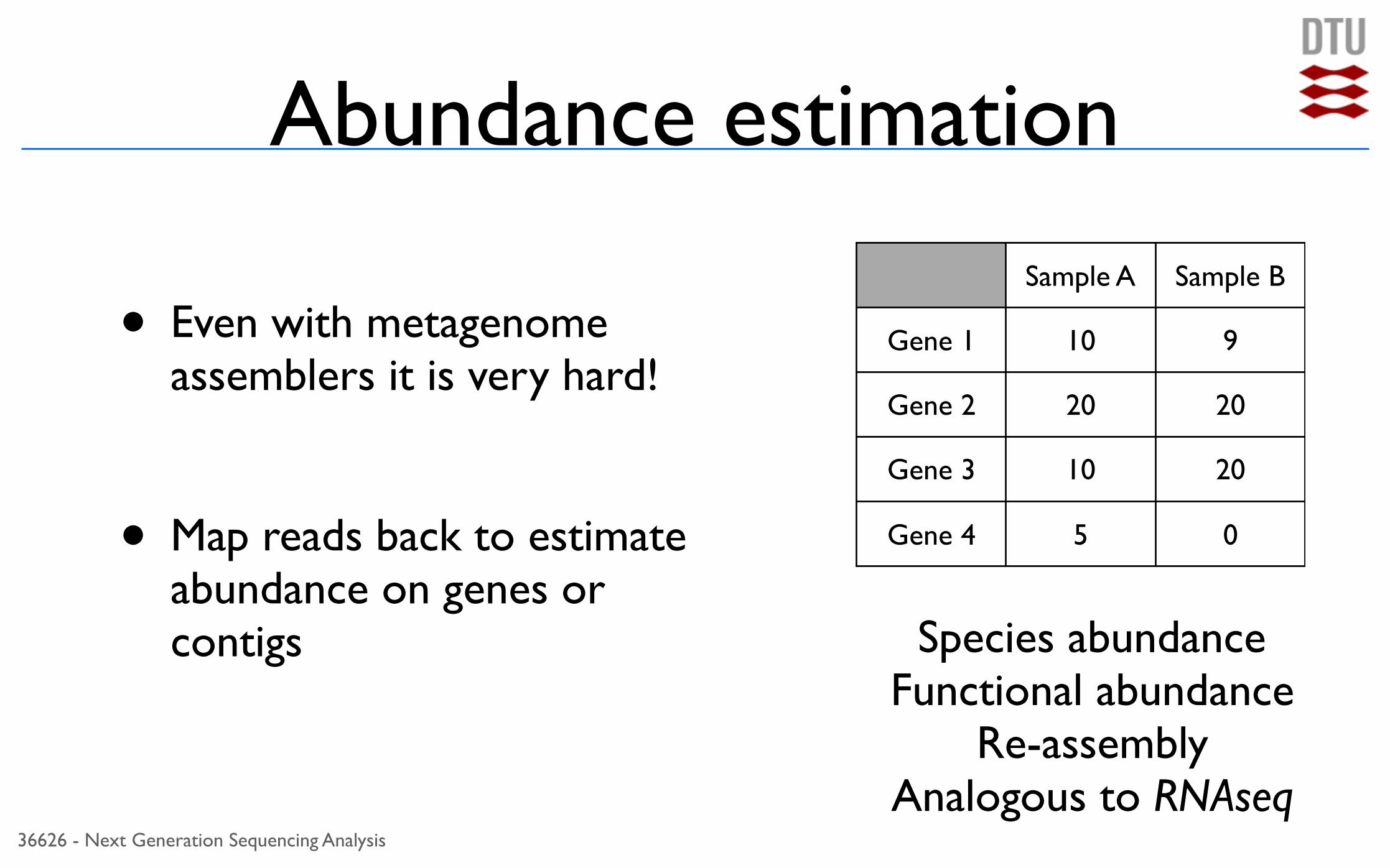
Abundance estimation

• Even with metagenome assemblers it is very hard!

• Map reads back to estimate abundance on genes or contigs

Sample A Sample B

Gene 1 10 9

Gene 2 20 20

Gene 3 10 20

Gene 4 5 0

Species abundanceFunctional abundance

Re-assemblyAnalogous to RNAseq


Binning

• Which contigs goes together?

• Binning:

• Similarity (alignment)

• Sequence composition & co-abundance of contigs (clustering)


Similarity (alignment)

• Align (BLAST/BWA) all contigs to reference database

• Quite accurate, but

• Databases are huge! and growing

• Majority of sequences are unknown (30%-99%)

• We can not find what is not there!


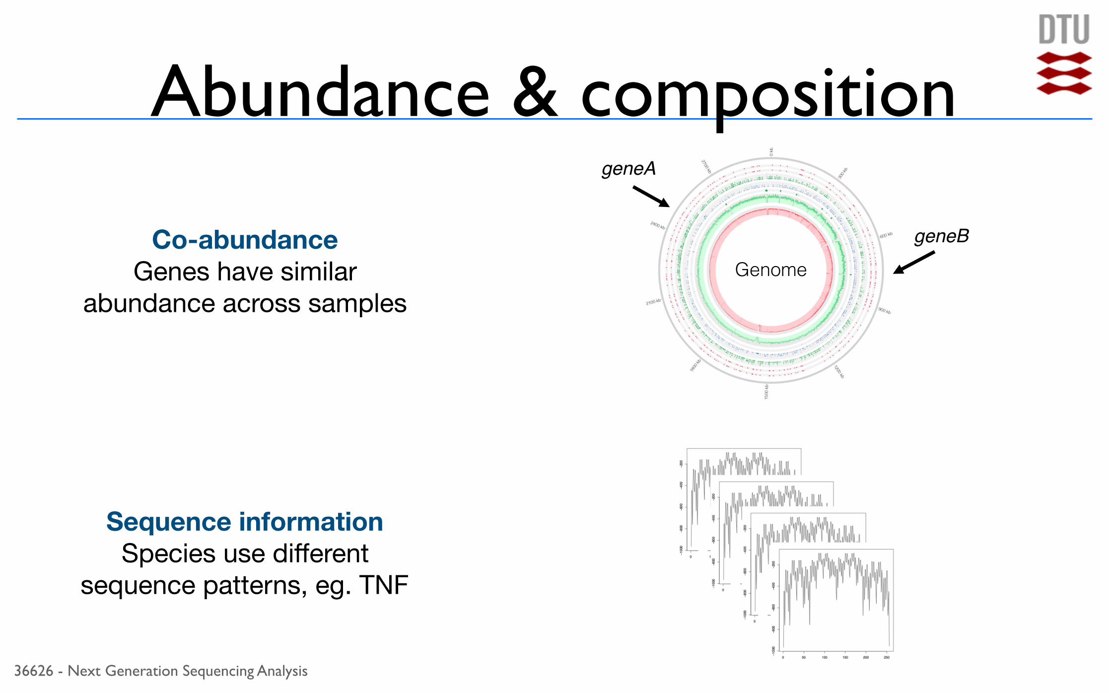
Abundance & compositiongeneA

geneB

GenomeCo-abundance

Genes have similar abundance across samples

Sequence information Species use different

sequence patterns, eg. TNF

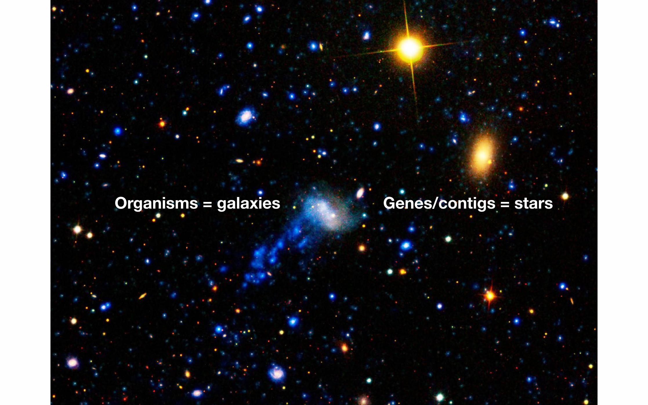
Genes/contigs = starsOrganisms = galaxies

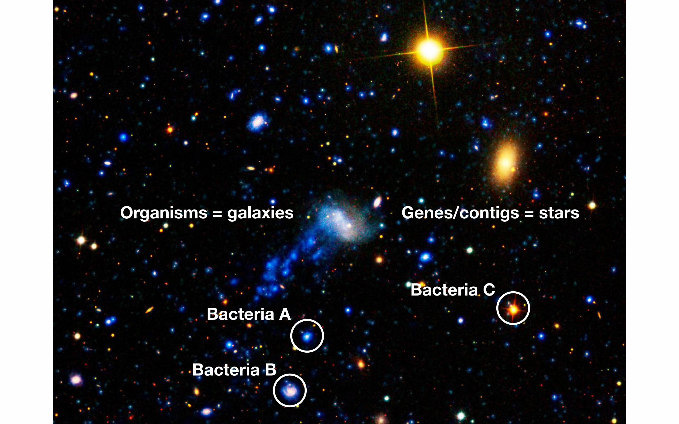
Genes/contigs = starsOrganisms = galaxies

Bacteria A

Bacteria B

Bacteria C

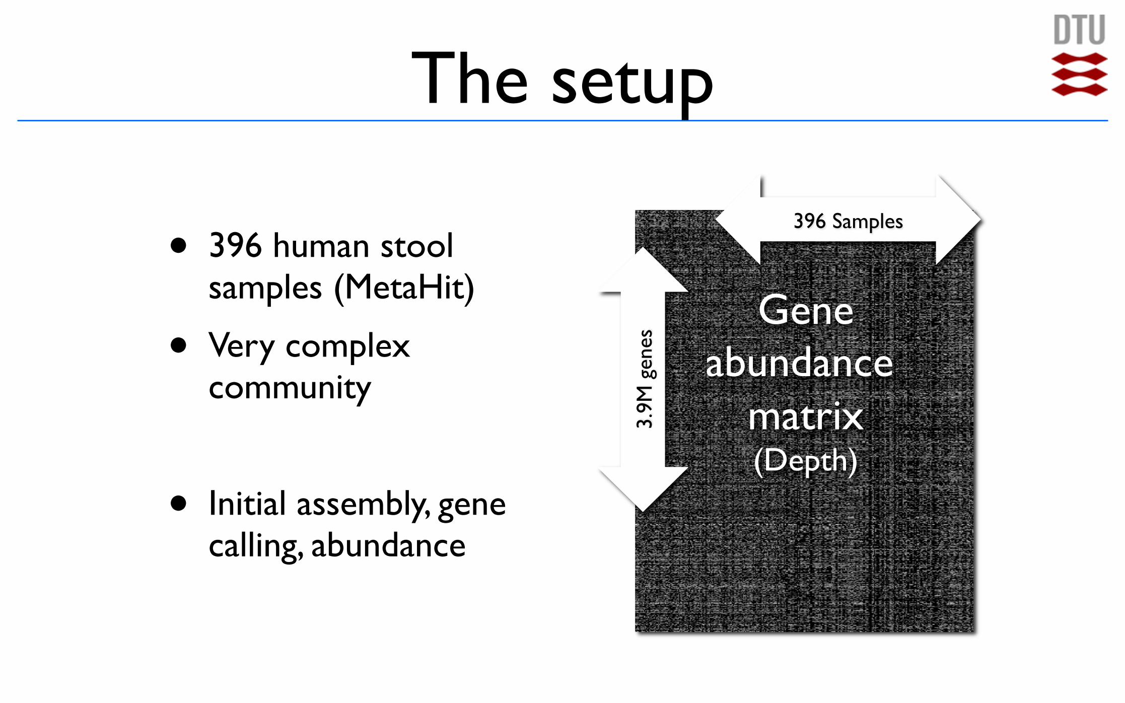
The setup

Gene!abundance

matrix!(Depth)

396 Samples

3.9M

gen

es

• 396 human stool samples (MetaHit)

• Very complex community

• Initial assembly, gene calling, abundance

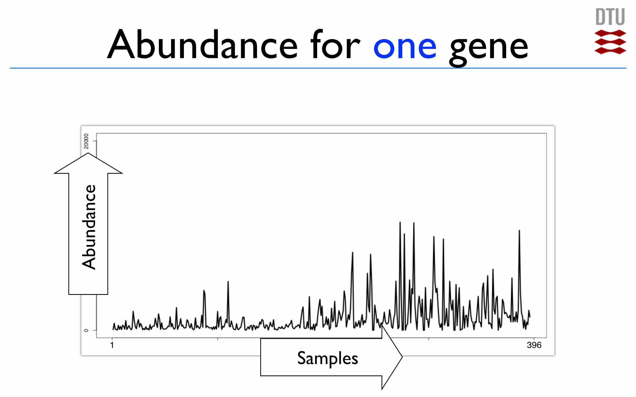
Abundance for one gene

1 396

Abu

ndan

ce

Samples

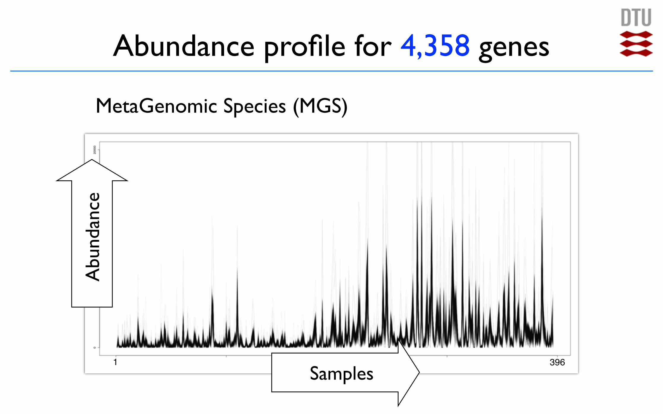
Abundance profile for 4,358 genes

1 396

Abu

ndan

ce

Samples

MetaGenomic Species (MGS)

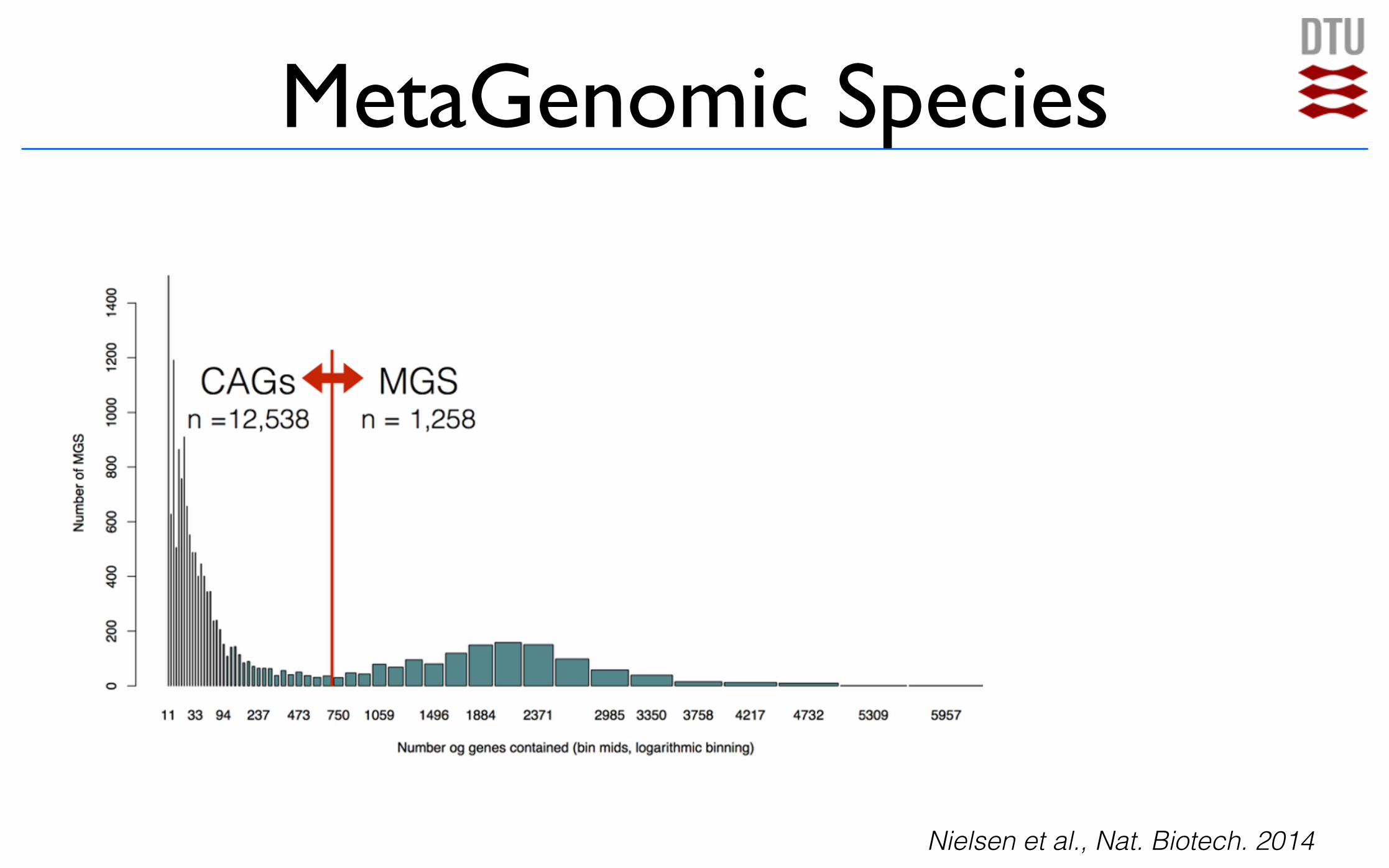
MetaGenomic Species

Nielsen et al., Nat. Biotech. 2014

Not just species gets binnedAlso plasmids and viruses... and lots of artifacts!

doi:10.1038/nbt.2939

Co-abundance groups vs metagenomic species


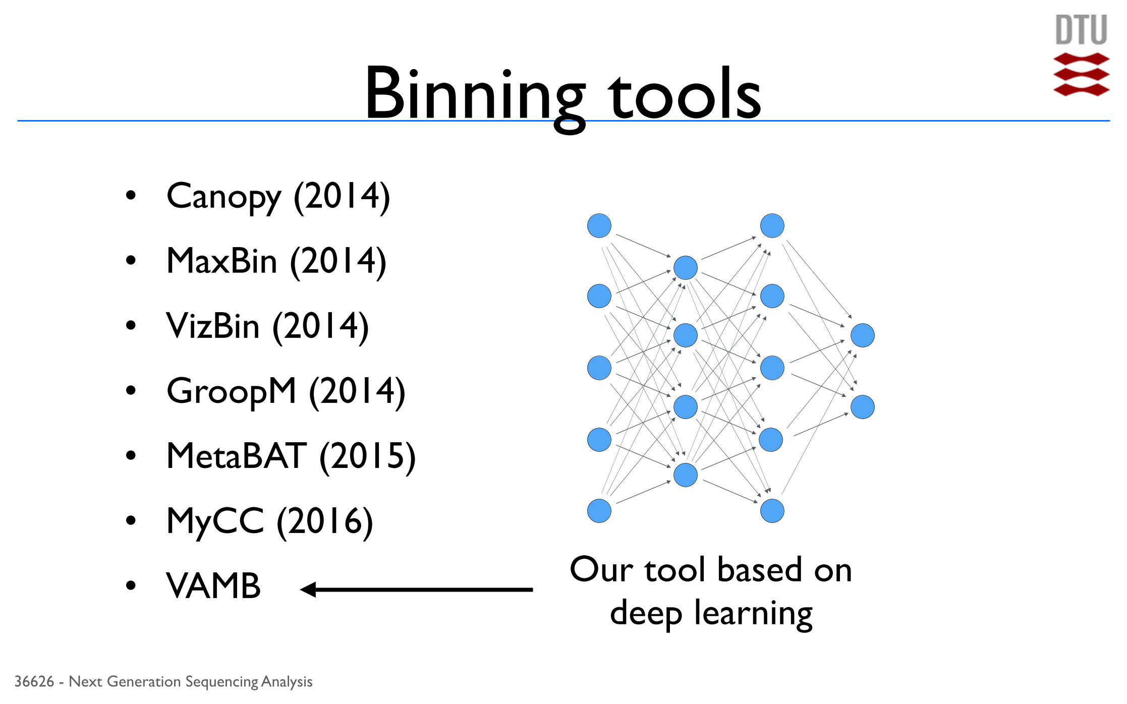
Binning tools• Canopy (2014)

• MaxBin (2014)

• VizBin (2014)

• GroopM (2014)

• MetaBAT (2015)

• MyCC (2016)

• VAMB Our tool based on deep learning

Documents

Metagenomics & metagenomic assembly ... - DTU … · Center for Biological Sequence Analysis ... Simon Rasmussen 36626: Next Generation Sequencing analysis DTU Bioinformatics. 36626