METALAB: A METABOLIC PROFILING DATABASE AND ANALYSIS TOOLKIT

by

MARK CHRISTOPHER WILSON

(Under the Direction of Chung-Jui Tsai)

ABSTRACT

Metabolic profiling is one of the pillars of functional genomics, and along with the development

of other omics tools for understanding cellular processes there has come a need for high throughput

metabolite matching that displays results in a visually intuitive way. A web-based pipeline called

MetaLab was developed to facilitate the storage, processing, analysis and retrieval of metabolite profiling

data. Retention index and mass spectral similarity coefficient are used for peak matching. Normalization

methods are available for assessing relative metabolite abundance for user-defined experimental groups.

Matched metabolite sets can be further explored using a variety of analytical and statistical tools. Export

of selected metabolites yields Excel spreadsheets displaying the alignment using a multi-color scheme.

MetaLab offers a platform that greatly simplifies manual curation of metabolite profiling data, allowing

researchers to focus more on the biological interpretation of their data.

INDEX WORDS: Metabolic; Profiling; Metabolite; Retention index; Similarity coefficient;

Database

METALAB: A METABOLIC PROFILING DATABASE AND ANALYSIS TOOLKIT

by

MARK CHRISTOPHER WILSON

BS, The University of Georgia, 2009

A Thesis Submitted to the Graduate Faculty of The University of Georgia in Partial Fulfillment of the

Requirements for the Degree

MASTER OF SCIENCE

ATHENS, GEORGIA

2012

© 2012

Mark Christopher Wilson

All Rights Reserved

METALAB: A METABOLIC PROFILING DATABASE AND ANALYSIS TOOLKIT

by

MARK CHRISTOPHER WILSON

Major Professor: Chung-Jui Tsai

Committee: Scott Harding

Liming Cai

Electronic Version Approved:

Maureen Grasso

Dean of the Graduate School

The University of Georgia

May 2012

iv

ACKNOWLEDGEMENTS

I would like to thank my advisors, Dr. Chung-Jui Tsai and Dr. Scott A. Harding, first and

foremost, for their continued support and patience during the time spent working with them. I cannot

express how much their expertise and guidance has helped me not only in my time spent under their

supervision, but also in the years to come. A special thanks is also extended to Dr. Liming Cai for his

support and encouragement over the past few years, as well as for accepting the duties of joining my

advisory committee.

I would also like to thank the many lab mates that have provided input on the features included

within this project. Over the course of my stay here, they have constantly provided guidance, feedback

and support. My friends at UGA have been overwhelming with their support for me as well.

My greatest appreciation goes out to my family. Without their unconditional love and support

over the years, the completion of my degree would not be possible.

v

TABLE OF CONTENTS

Page

ACKNOWLEDGEMENTS ......................................................................................................................... iv

CHAPTER

1 INTRODUCTION ..................................................................................................................... 1

2 MATERIALS AND METHODS .............................................................................................. 5

Server Software ................................................................................................................... 5

GC-MS Data Acquisition & Processing ............................................................................. 5

AnalyzerPro ........................................................................................................................ 6

AMDIS................................................................................................................................ 6

Terminologies ..................................................................................................................... 7

Data Formats and Requirements ......................................................................................... 8

3 RESULTS ................................................................................................................................ 10

Overall User Goal ............................................................................................................. 10

Peak Alignment by Similarity Coefficient ........................................................................ 10

Peak Alignment by Retention Index ................................................................................. 12

Database Backend ............................................................................................................. 13

Data Upload ...................................................................................................................... 14

Data Storage and Backup .................................................................................................. 15

Quality Check for RI and IS Markers ............................................................................... 16

Creating an Experiment for Analysis ................................................................................ 16

Data Analysis and Interpretation ...................................................................................... 19

Metabolite Detail Reports ................................................................................................. 21

Search Function ................................................................................................................ 21

vi

Viewing Existing Experiments ......................................................................................... 22

Database Administration and User Authentication ........................................................... 22

4 DISCUSSION ......................................................................................................................... 23

Automated Features .......................................................................................................... 23

Analysis and Data Display Features ................................................................................. 24

System Management ......................................................................................................... 25

Data Optimization ............................................................................................................. 26

Future Improvements ........................................................................................................ 26

5 CONCLUSION ....................................................................................................................... 27

ACKNOWLEDGEMENTS ........................................................................................................................ 42

1

CHAPTER 1

INTRODUCTION

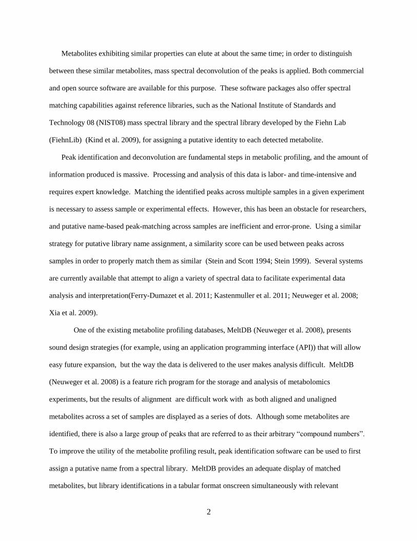
In order to fully understand the various chemical processes occurring at the cellular level,

researchers have recently began focusing on the chemical constituents within a cell at a certain point in

time. Taking a “snapshot” can allow researchers to piece together a larger biological picture. Profiling

these chemical constituents, or metabolites, can provide a quantitative as well as qualitative description of

the cellular metabolism under investigation (Fiehn 2002). Metabolite profiling has emerged as a reliable

tool in linking findings on the genomic, transcriptomic or proteomic levels (Bino et al. 2004). Such

profiling techniques are not kingdom specific – recent metabolic profiling studies have ranged from

diseases in wasps (Colinet et al. 2012) to reproduction in grasses (Rasmussen et al. 2012).

A variety of analytical techniques are available for metabolic profiling. The most common

method is Gas Chromatography-Mass Spectrometry (GC-MS), which is considered the gold standard in

metabolomics (Dunn and Ellis 2005). GC-MS is essentially a way to separate the complex metabolic

makeup of a sample based on the differences in the volatility of the individual metabolites. Samples are

usually chemically modified to enhance volatility, and then heated to a temperature that vaporizes, but

only minimally decomposes the constituent metabolites. Once in a gaseous state, these metabolites travel

the length of a chromatography column, where they interact with the matrix of the column. Once the end

of the column is reached, the metabolite elutes out of the column at a set time, noted as the retention time

that is characteristic of that metabolite. The eluted metabolite then enters the mass spectrometer, where it

is ionized, or bombarded with electrons, generating multiple „ion fragments‟ per metabolite. The mass-

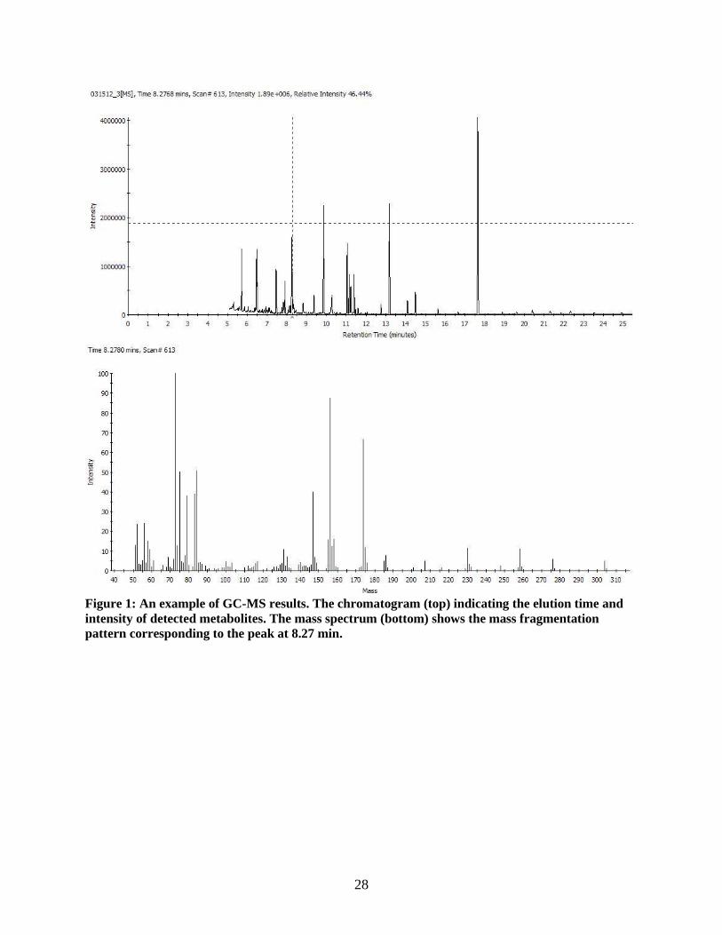
to-charge ratios of the fragments are then recorded. The GC-MS output data is therefore reported in a

two-tier format – a chromatogram depicting the elution (retention) times of the metabolites, as well as the

corresponding ion fragmentation profile (mass spectrum) for each of the metabolites on the

chromatogram (Figure 1).

2

Metabolites exhibiting similar properties can elute at about the same time; in order to distinguish

between these similar metabolites, mass spectral deconvolution of the peaks is applied. Both commercial

and open source software are available for this purpose. These software packages also offer spectral

matching capabilities against reference libraries, such as the National Institute of Standards and

Technology 08 (NIST08) mass spectral library and the spectral library developed by the Fiehn Lab

(FiehnLib) (Kind et al. 2009), for assigning a putative identity to each detected metabolite.

Peak identification and deconvolution are fundamental steps in metabolic profiling, and the amount of

information produced is massive. Processing and analysis of this data is labor- and time-intensive and

requires expert knowledge. Matching the identified peaks across multiple samples in a given experiment

is necessary to assess sample or experimental effects. However, this has been an obstacle for researchers,

and putative name-based peak-matching across samples are inefficient and error-prone. Using a similar

strategy for putative library name assignment, a similarity score can be used between peaks across

samples in order to properly match them as similar (Stein and Scott 1994; Stein 1999). Several systems

are currently available that attempt to align a variety of spectral data to facilitate experimental data

analysis and interpretation(Ferry-Dumazet et al. 2011; Kastenmuller et al. 2011; Neuweger et al. 2008;

Xia et al. 2009).

One of the existing metabolite profiling databases, MeltDB (Neuweger et al. 2008), presents

sound design strategies (for example, using an application programming interface (API)) that will allow

easy future expansion, but the way the data is delivered to the user makes analysis difficult. MeltDB

(Neuweger et al. 2008) is a feature rich program for the storage and analysis of metabolomics

experiments, but the results of alignment are difficult work with as both aligned and unaligned

metabolites across a set of samples are displayed as a series of dots. Although some metabolites are

identified, there is also a large group of peaks that are referred to as their arbitrary “compound numbers”.

To improve the utility of the metabolite profiling result, peak identification software can be used to first

assign a putative name from a spectral library. MeltDB provides an adequate display of matched

metabolites, but library identifications in a tabular format onscreen simultaneously with relevant

3

statistical data such as normalized areas and p-value would enhance user experience. Onscreen sorting of

the results would also be helpful to the user. MetaboAnalyst (Xia et al. 2009) is compatible with a variety

of input data formats derived from different analytical platforms such as NMR-MS, LC-MS and GC-MS

data. It is feature-rich in analytical tools that include Principal Component Analysis (PCA), various types

of heat maps, and uni- and multi-variate analysis, but the program was difficult to navigate and did not

appear to have peak identification functionality against a spectral library. The MetaboAnalyst package

has simple GC-MS and LC-MS functionality, but focuses most of its resources on NMR-MS data

analysis.

A more recent metabolomics experiment server, metaP (Kastenmuller et al. 2011), has attempted

to simplify alignment of multiple samples (i.e., their associated metabolites) within an experiment. It

provides a simple and easy-to-navigate user interface, but it is limited in analysis tools and data detail.

The metabolite list is simple, displaying only peak area values along with standard deviations. The main

metabolite page does provide links to individual metabolite information. The analysis summary lists

metabolites by their Kit-IDs with statistical data concerning peak area. PCA graphs are available, and

users are able to perform hypothesis tests and download p-value outputs. The putative identification can

be viewed in detail, and links (if applicable) to other databases are listed based on KEGG, BioCyc, and

PubChem IDs, to name a few. MetaP only accepts Biocrates MetIQ data, a commercial kit and software

package designed for targeted metabolomics identification in plasma samples. As such, the metaP

software package is tailored specifically to Biocrates kit users, with limited applicability to the broader

user community.

Metabolite profiling has been adopted in the Tsai laboratory as part of a functional genomics

research program focusing on Populus (Jeong et al. 2004, Harding et al. 2005). The concept of MetaLab

was born out of necessity as more graduate students and researchers in the lab applied metabolite

profiling to their own research. A prototype was developed by former researchers but the system lacked a

standard database structure. The execution of simple experiments with large numbers of samples

overwhelmed the system. The current project aimed to reduce manual processing and inspection time of

4

metabolite profiling data, employ a system for backup and storage of the data, and provide automated

tools for statistical analysis in a simplified and easy-to-use format. MetaLab attempts to streamline peak

matching across multiple samples by using a combination of criteria that consider retention time index,

mass spectral similarity coefficient, and metabolite grouping confidence. The development and

improvements of MetaLab have been driven by user need and feedback. Every attempt has been made to

preserve simplicity while increasing productivity of the researcher.

5

CHAPTER 2

MATERIALS AND METHODS

Server Software

The MetaLab package was tested on a dedicated server with two Pentium® D 3.0 GHz processors

and 8 GB RAM running Ubuntu Linux (http://www.ubuntu.com, 64-bit Server Edition). Ubuntu versions

9.04-11.10 have been successfully tested.

The MetaLab onscreen display is created using a combination of PHP 5.3 (http://www.php.net)

and MySQL 5.1 (http://www.mysql.com) on an Apache 2 (http://www.apache.org) web server. The

MySQL database engine is used to store sample and experiment data using relationally linked tables.

Graphs and plots are generated using JpGraph PHP graphing library (http://www.jpgraph.com).

GC-MS Data Acquisition & Processing

The GC-MS data used for MetaLab development were obtained using an Agilent 7890A Gas

Chromatograph coupled to a 5975 Series Mass Spectrometer (Agilent Technologies, Wilmington, DE).

Plant extracts were derivatized and analyzed by GC-MS essentially as described (Jeong et al. 2004), with

modified oven temperature ramp rates (from 80oC to 200

oC at 20

oC min

-1 and from 200

oC to 310

oC at

10oC min

-1), and a shortened total runtime of 25.5 min. A scan range of 50 to 500 m/z was used with a

scan rate between 2-4 sec-1

. Data was collected using the ChemStation software v.E.02.00.493 (Agilent

Technologies). Using a peak deconvolution and identification software package, such as the AnalyzerPro

(SpectralWorks) or the AMDIS (The Automated Mass Spectral Deconvolution and Identification

System), alongside the NIST08, Fiehnlib or in-house mass spectral libraries, peaks were assigned putative

identities using the following parameters.

6

AnalyzerPro

GC-MS data acquired from the ChemStation software is post-processed mainly using

AnalyzerPro ver. 2.5.0.0 (SpectralWorks). The following method variables were used:

Min Masses: 3

Area Threshold: 100

Height Threshold: 0

Signal to Noise: 2

Width Threshold: 0.01 min

Resolution: Very Low

Scan Window: 3

Smoothing: 3

Library Searching was enabled and a total of three libraries were used for assigning a putative

identity to each metabolite:

National Institute of Standards and Technology (NIST) 2008 Mass Spectral Library

(Babushok et al. 2007)

FiehnLib provided by Agilent Technologies (Kind et al. 2009)

In-house library of authentic standards

The minimum confidence for naming a peak was set at 40%. The minimum confidence score was

defined in AnalyzerPro as: (0.7 x Reference Library Forward Match percentage) + (0.3 x Reference

Library Reverse Match percentage) (SpectralWorks).

AMDIS

GC-MS data can also be processed using AMDIS (ver. 2.66), a non-commercial deconvolution

and peak identification software package (Davies 1998). The “Minimum Match Factor” was set to 70.

7

The “All Above Threshold”, or the minimum signal recorded by the instrument, was set to 0.005

(AMDIS).

Terminologies

The following definitions are provided for terminologies used throughout:

Sample – A set of metabolites from a single GC run.

Group – A set of data samples, typically a set of replicates that are included together by

the user in order to make statistical comparisons between groups for a given experiment.

Experiment – A set of samples, typically associated with multiple user-defined groups to

address specific research questions, such as comparison across genotypes or treatments.

Metabolite – A peak identified and assigned a name by the library search function of

AnalyzerPro or AMDIS.

Matched Metabolite Set – A set of peaks, each from different samples of a defined

experiment that have been grouped based on peak-alignment criteria and identified as representing the

same metabolite across the samples.

Retention Time (RT) – the time it takes for a vaporized metabolite to travel through and

elute out of the column into the mass detector.

Retention Index (RI) – a regression of molecular size on RT that can be used to normalize

RT values that deviate over time due to column shortening and performance changes. RI was calculated

using the retention times of a series of n-alkane molecular size markers: pentadecane @ 1500, eicosane @

2000, pentacosane @ 2500, and triacontane @ 3000 - (Ettre 1993).

8

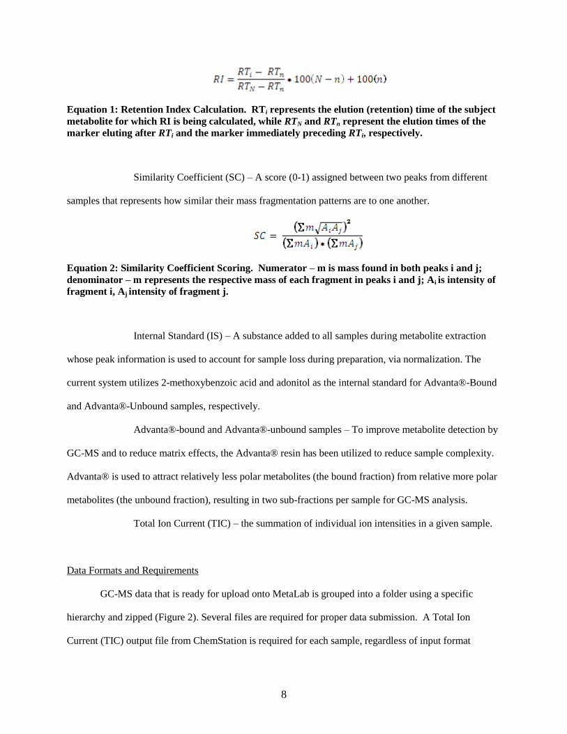
Equation 1: Retention Index Calculation. RTi represents the elution (retention) time of the subject

metabolite for which RI is being calculated, while RTN and RTn represent the elution times of the

marker eluting after RTi and the marker immediately preceding RTi, respectively.

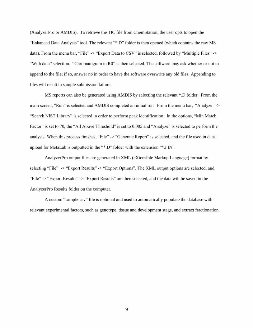
Similarity Coefficient (SC) – A score (0-1) assigned between two peaks from different

samples that represents how similar their mass fragmentation patterns are to one another.

Equation 2: Similarity Coefficient Scoring. Numerator – m is mass found in both peaks i and j;

denominator – m represents the respective mass of each fragment in peaks i and j; Ai is intensity of

fragment i, Aj intensity of fragment j.

Internal Standard (IS) – A substance added to all samples during metabolite extraction

whose peak information is used to account for sample loss during preparation, via normalization. The

current system utilizes 2-methoxybenzoic acid and adonitol as the internal standard for Advanta®-Bound

and Advanta®-Unbound samples, respectively.

Advanta®-bound and Advanta®-unbound samples – To improve metabolite detection by

GC-MS and to reduce matrix effects, the Advanta® resin has been utilized to reduce sample complexity.

Advanta® is used to attract relatively less polar metabolites (the bound fraction) from relative more polar

metabolites (the unbound fraction), resulting in two sub-fractions per sample for GC-MS analysis.

Total Ion Current (TIC) – the summation of individual ion intensities in a given sample.

Data Formats and Requirements

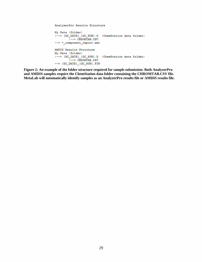
GC-MS data that is ready for upload onto MetaLab is grouped into a folder using a specific

hierarchy and zipped (Figure 2). Several files are required for proper data submission. A Total Ion

Current (TIC) output file from ChemStation is required for each sample, regardless of input format

9

(AnalyzerPro or AMDIS). To retrieve the TIC file from ChemStation, the user opts to open the

“Enhanced Data Analysis” tool. The relevant “*.D” folder is then opened (which contains the raw MS

data). From the menu bar, “File” -> “Export Data to CSV” is selected, followed by “Multiple Files” ->

“With data” selection. “Chromatogram in R0” is then selected. The software may ask whether or not to

append to the file; if so, answer no in order to have the software overwrite any old files. Appending to

files will result in sample submission failure.

MS reports can also be generated using AMDIS by selecting the relevant *.D folder. From the

main screen, “Run” is selected and AMDIS completed an initial run. From the menu bar, “Analyze” ->

“Search NIST Library” is selected in order to perform peak identification. In the options, “Min Match

Factor” is set to 70, the “All Above Threshold” is set to 0.005 and “Analyze” is selected to perform the

analysis. When this process finishes, “File” -> “Generate Report” is selected, and the file used in data

upload for MetaLab is outputted in the “*.D” folder with the extension “*.FIN”.

AnalyzerPro output files are generated in XML (eXtensible Markup Language) format by

selecting “File” -> “Export Results” -> “Export Options”. The XML output options are selected, and

“File” -> “Export Results” -> “Export Results” are then selected, and the data will be saved in the

AnalyzerPro Results folder on the computer.

A custom “sample.csv” file is optional and used to automatically populate the database with

relevant experimental factors, such as genotype, tissue and development stage, and extract fractionation.

10

CHAPTER 3

RESULTS

Overall User Goal

The goals of MetaLab are to provide the user with a simple data analysis pipeline to align

deconvoluted metabolic profile data from different samples using similarity coefficients and a retention

index, and then to offer accessory tools to analyze treatment or genotype effects on metabolism. In order

to achieve this, MetaLab presents its graphical user interface (GUI) via a web browser; as such, it avoids

cross-platform limitations. Remote installation of MetaLab to a centralized web server eliminates the need

for releases on multiple platforms (i.e., Microsoft ® Windows, Apple ® OS) as browsers have begun

using standardized rules on how browsers interpret web pages. This also avoids complications with

software dependencies differing from platform to platform. All of the software used in MetaLab has been

selected for its ease of use, portability, popularity, and open source licensing.

Peak Alignment by Similarity Coefficient

Peak matching lies at the crux of profile alignment and occurs as a one-to-one comparison of

constituent peaks based on their mass spectral properties. Putative identities (names) assigned by peak

identification software (AnalyzerPro or AMDIS) upstream of MetaLab are not used in the alignment

process. In other words, nomenclature does not play a part in peak matching between samples, but the

MS fragmentation pattern associated with the identified peak (metabolite) does. The similarity coefficient

(SC) algorithm (Equation 2) adopted in MetaLab is similar to those used in the library searching process

for assigning putative identities to unknown peaks based entirely on their MS fragmentation patterns

(Lam et al. 2007; Stein and Scott 1994). Peak matching results across all samples in a given experiment

are used for de novo grouping of metabolites, one at a time, but a priori (biological) sample information is

11

not considered at this stage. Grouping of aligned peaks is based on several criteria. Beginning with the

first sample in the given analysis, each candidate peak is compared with other peaks in subsequent sample

files (one at a time) within a specified retention index (RI) range, and a SC score is assigned to each

pairwise comparison. The SC algorithm is weighted in favor of the fragment ions that are common

between peaks, but penalizes those that are found within only one of the peaks. The RI range is based on

empirical testing, and for the data examined, a window of ± 50 units has been found optimal. This is

equivalent to roughly 1.5% of the average RI value in our datasets. This RI window improves the

computational performance of the peak-matching step by reducing the number of candidate pairs and

calculations between all possible matches.

Candidate peaks passing the user-defined SC score cutoff are assigned to a metabolite group

based on a second parameter called “group consistency”. By default, the group consistency is set at 60%.

If the group size is less than five, the group consistency is not in effect. In that case, grouping for the first

four samples occurs as long as the respective peaks are within the RI window and have an SC score above

the cutoff for at least one pair of peaks in the matched metabolite set. When the group size is greater than

four, the peak in question must lie within the RI window and have the similarity coefficient score above

the cutoff for at least 60% of the pairwise comparisons against all samples in the current group for it to be

accepted into the group. If two or more peaks from the same sample match these criteria, the peak with

the maximal similarity coefficient score is selected. The group consistency parameter reduces the number

of inaccurate peak matches by ensuring that a matched metabolite set has an acceptable scoring pattern

with a majority of samples within the current group. This is because erroneous group assignment can

occur by chance. By using the majority rule as the basis for joining a matched set, inaccurate peak

matching is reduced.

12

Peak Alignment by Retention Index

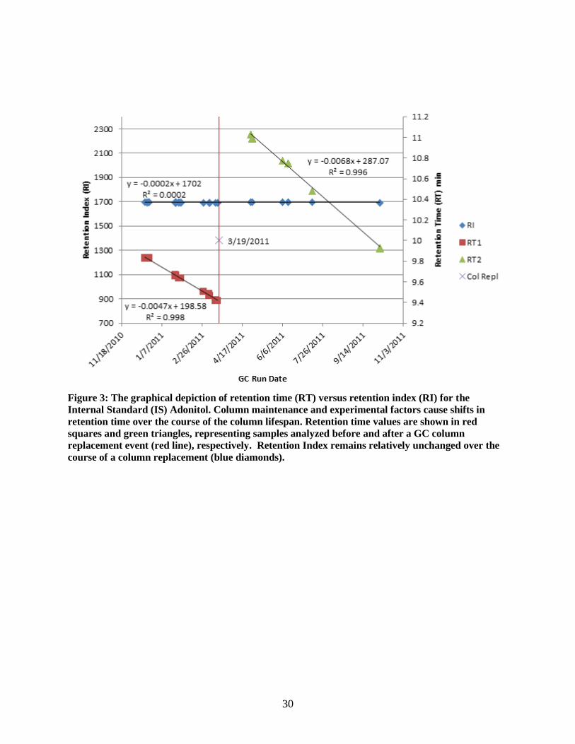
Environmental and regular maintenance to the GC-MS machine are known to cause drifting of

the retention times of metabolites (Ettre 1993). This can become a source of error in peak matching when

retention time is considered. Experimental data (Figure 3) showed that retention time fluctuation occurs

over time due to performance drift and scheduled GC-MS maintenance procedures. In particular, there is

a gradual decrease in retention time of a given compound as the column is trimmed, until such time when

the column is replaced, with a sudden increase in retention time, and the cycle repeats. For samples that

are analyzed by GC-MS within a short time window of less than one or two weeks, the retention time

drift may have a minimal effect on peak matching; thus, an experiment relying on RT as the reference

time window would be acceptable under ordinary circumstances. However, the comparison of two peaks

representative of the same metabolite from two dates spanning the life of the column would exhibit

retention time drift, and normalization of the retention time is necessary. Retention time drift also occurs

with slight differences in instruments as well as differences in methods from lab to lab.

A retention index calculation is attempted for every metabolite in each sample uploaded to

MetaLab. Although experiments can be created and analyzed using retention time as the basis for peak-

matching (i.e., a user-defined RT window), retention index has been shown to provide a more stable

measure of the retention property, and hence increase accuracy of peak matching. An added benefit for a

more stable RI parameter is that the time window for peak-matching can be further reduced, thereby

decreasing computational time during peak-matching analysis. The initial retention index marker

identification and calculation is automated in MetaLab upon data submission, using pre-defined

parameters based on lab-specific protocols and GC method. Each GC method has a defined RT window

for each of the alkane markers. This window can be determined empirically and adjusted by the

administrator as needed. As markers may be mis-identified in the automated pipeline, due to a variety of

technical or biological reasons, it is highly recommended that the user check the automated marker

selection for accuracy. MetaLab provides two options (during data submission and parsing stage) to

assist with the manual correction process, when one or more RI markers are missing. The user can assign

13

markers using an average from runs that occurred on the same day, as RT drift is negligible across these

samples. Alternatively, the user can inspect and select the missing marker(s) or their proxies manually.

In addition, the User Access Panel allows users to browse existing sample files and view/edit previously

defined markers as necessary.

Database Backend

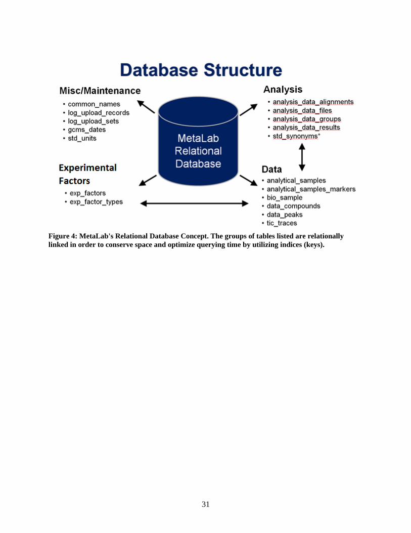
MetaLab is operated on the MySQL ver. 5.1 (http://www.mysql.com/) database engine. It

incorporates a relational database schema, with InnoDB type tables (Figure 4). The benefits of a

relational database design include optimization of storage space and efficient data insertion and retrieval.

In order to maintain standards and accurate record insertion, transactions are used when inserting data or

when an experiment is created. This ensures that no orphaned records are present within the database

system. Orphaned records waste space and can cause integrity checks to produce false errors. For non-

relational tables, the MyISAM format was chosen for speed and does not incorporate ACID standards

(Haerder and Reuter 1983), while InnoDB tables were chosen to avoid mismatched and orphaned records

and to maintain ACID standards. ACID standards guarantee that database modifications are reliable by

updating in an all-or-none manner for linked-table queries. Tables within the MetaLab database that do

not require adherence to ACID standards are of the MyISAM format.

The current database configuration of MetaLab consists of 30 tables. Sample data storage uses six

of these tables, each with InnoDB database format. Creation of an experiment uses another six tables,

also in the InnoDB format. One of these tables is used as a cache and stores similarity coefficient scores

of previously calculated values between peaks. By storing the SC values, the system avoids redundant

calculations for previously aligned peaks, thereby reducing computational wait time during experiment

creation or re-analysis. Two tables are designated for logging data upload failures. This has been useful

in issues associated with format errors in the exported data from AnalyzerPro and AMDIS. A common

names table holds a list of roughly 2700 metabolites and their corresponding parent names. The

compound name is substituted for its common name if available.

14

MetaLab‟s structure was designed to allow flexibility in the number of retention and internal

markers used in each analysis. System administrators are able to add and manipulate these markers from

the Database Administration menu. The database tables for both retention time and internal standard

markers are relational, eliminating duplicate data as both these marker types are linked to several

experimental factors independent of one another. For example, when the parameters of the GC-MS

analysis are changed, a new GC Method can be defined in the database. By incorporating the relational

database structure for the marker types, easy expansion for future experiments is possible without the

need of essentially doubling the records every time a new experimental GC method is implemented.

Data Upload

MetaLab accepts GC-MS data that has been deconvoluted using either AnalyzerPro or AMDIS

software packages. Both a free and commercial software option are presented to better suit the end user,

and these packages have been compared for reliability and credibility (Lu et al. 2008). MetaLab needs

additional data from ChemStation in order to recreate chromatogram overlap graphs as part of the detailed

report and quality control functions. The chromatogram overlap helps identify outlier samples within the

matched metabolite set by visually comparing the preprocessed data.

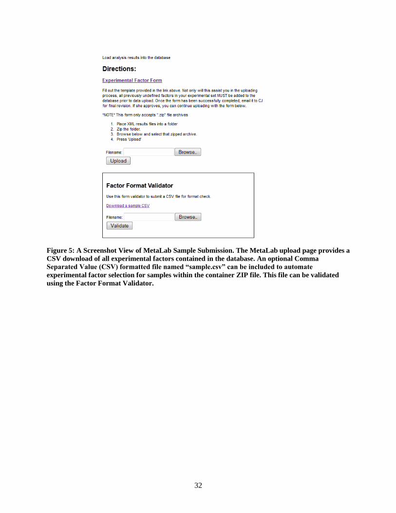
Experimental data is submitted to MetaLab by using the Data Upload menu (Figure 5). Prior to

upload, it is required that a user ensure all experimental factors in the given experiment are listed on the

Experimental Factor Form, available on the data upload page. Experimental factors not present on the

form will not be accepted by MetaLab, but can be added by the administrator upon approval of the Lab

PI. This is intended to standardize vocabularies in the database and to facilitate subsequent information

retrieval. Experimental data is then compiled into a folder in the hierarchal structure seen in Figure 2.

Each sample is required to have an output results file either in AnalyzerPro or AMDIS format and the

ChemStation raw data folder, which includes the total ion current (TIC) chromatogram data

(CHROMTAB.CSV). The ChemStation raw data folder (*.D), may contain other files, but only the

CHROMTAB.CSV is required. AnalyzerPro or AMDIS outputs can be included within a single folder.

15

An optional “sample.csv” file can be included to allow automated population of experimental factors into

the database without manually entering these factors, one sample at a time. This folder is then zipped,

and the data can be uploaded using the Data Upload function (Figure 5).

Once MetaLab has processed the zip file contents, it will report and remove any samples that do

not have all of the required data files or samples that are already stored in the database. MetaLab will

also automatically determine incomplete data and produce a warning report with these file names, while

continuing on with any that are complete. MetaLab will also report back to the user any samples that are

missing RI or IS markers during this process. To minimize user confusion, the backend also sorts the

files in ascending order, eliminating system sort limitations. For example, by default, AnalyzerPro outputs

results files by appending a run number to the GC run date (i.e., 031812_11). Rather than filing 11 after 1,

MetaLab keeps the file order as one would expect with ascending order. Other limitations to AnalyzerPro

are also overcome automatically by MetaLab, such as incorrect parsing of XML results files. In

AnalyzerPro ver. 2.5.0.0, names are sometimes given that contain XML-restricted characters, “>” and

“<”. By default, this returns a fatal error by the XML parser in PHP. MetaLab has a built-in feature that

automatically checks for and corrects improper XML formatting. The user is then presented with a set of

forms corresponding to the number of valid samples for defining/entering their associated experimental

factors manually. Alternatively, if a pre-filled “sample.csv” file is also submitted in the zipped folder, the

experimental factors will be automatically populated. A biological sample identification number that

allows the user to quickly identify the sample is the only required field, but it is recommended that all

other fields are reported accurately for search purposes.

Data Storage and Backup

Data uploaded to MetaLab is stored within the MetaLab /tmp/ directory. Administrators have the

option of automatically backing up the uploaded data to a remote storage option via a cron script. The

„backup_files.sh‟ script found within the cron folder of MetaLab must be edited with the corresponding

16

details, a SSH key handshake must be configured between the two machines, and the said script will

securely copy all data to the remote backup server.

Administrators are also provided a script to back up the MySQL database. The script located in

the cron folder, „mpdbdump.sh‟, will extract the database to a temporary directory as defined within the

script. The database backups are automatically archived for file compression using gzip, and the file is

time stamped with the backup time and date.

By archiving and saving uploaded data sets, MetaLab essentially provides an integrated data

backup solution for the original data generated from GC-MS.

Quality Check for RI and IS Markers

Upon data submission, MetaLab will unpackage the zipped folder, parse the data files and store

the experimental factor information into the relevant tables in the database. MetaLab attempts to

automatically identify retention index and internal standard markers according to the specific GC-MS

method. It is highly recommended that every user checks the results of the automated index identification

for accuracy. The automated process can yield misidentification of markers due to unusual RT shifts

(outside of the pre-defined RT window) or other sample-specific matrix effects. Using the User Access

Panel, MetaLab users are able to update, add or delete markers either on a “per day-per run” or on a “per

sample” basis. The “per day-per run” option allows multiple sample files run on the same day (with the

same ChemStation date in their file names) to be edited together. This is because daily GC runs typically

exhibits negligible retention time drift when comparing metabolites across samples. MetaLab provides

the user the option to use an average RT value for each RI marker that is calculated from samples run on

that particular day.

Creating an Experiment for Analysis

Users are able to create an experiment in order to identify metabolite responses across samples.

These samples can be assigned to different groups in accordance with the experimental design, such as

17

different genotype, tissue or treatment groups, with group members typically represent biological

replicates. This sample grouping is important as it is the basis for subsequent calculation of group

average and standard deviation, and for other downstream statistical analyses.

To perform an experiment analysis, a registered user selects „Create Experiment‟ tab from the

menu. A title and brief description are required. Users are able to dynamically create groups in which to

place their replicates. This is done using the scriptaculous JavaScript library (http://script.aculo.us/) in

combination with a modified demo (http://www.gregphoto.net/sortable/advanced/). Groups can be named

to reflect their nature, such as genotypes, tissues, treatments or any combinations; files can then be

dragged into the respective groups.

Expert parameters can be adjusted in order to optimize results. The peak alignment method can

either be RI- or RT-based, the latter in the event retention index markers are purposely omitted. The peak

intensity cutoff allows the user to eliminate low-intensity peaks as background noise during the peak

alignment. The Spec Sim is the user-selected cutoff of the similarity coefficient when peak matching

occurs. The group consistency represents the minimum percentage (in decimal form) of the candidate

group members against which the peak‟s similarity coefficient score must satisfy the Spec Sim.

Once the experiment has been submitted, it will be placed into a queuing system. This is

implemented in order to avoid having the user wait while the analysis is underway, which, depending on

the experiment and sample number, may take up to five hours to complete. It also eliminates the potential

of analysis corruption by the user stopping the browser or refreshing the page inadvertently. The queuing

system displays an estimated time for each analysis in the queue, as well as the runtime of the current

analysis being processed. Estimated times are calculated using a linear regression model of the actual run

time of previously performed analyses and the number of ion fragments present in each analysis.

Once the analysis has been processed, users are presented with a summary table of the resulting

peak alignment. The alignment parameters and sample information for each experiment are displayed at

the top of the page. Hyperlinks provide convenient access to individual samples for manual examination.

Users can select among different data normalization methods and the results will be re-calculated on the

18

fly and the display updated. Norm TIC refers to normalization of the peak area to the total ion

chromatogram value (TIC) in that sample. Norm IS refers to the normalization of the peak area to the area

of the Internal Standard (IS). These values can be further adjusted by the sample dry weight used for the

initial metabolite extraction (default to 10 mg currently).

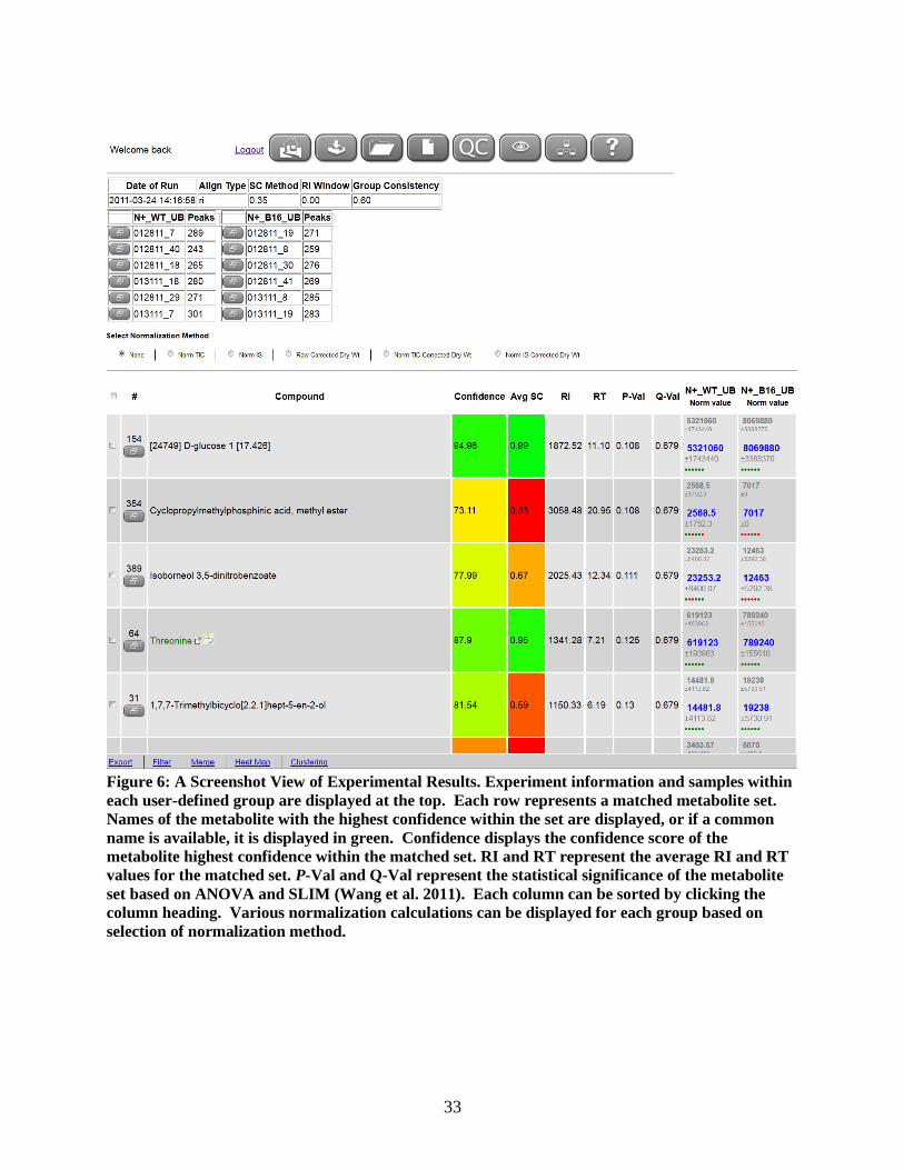
Each row represents a matched metabolite set across the samples within the experiment (Figure

6). Columns within this table can be sorted alphabetically or numerically by simply clicking the column

heading. The name of the matched set is extracted from the library search results (by AnalyzerPro or

AMDIS), based on the metabolite having the highest confidence score among the matched set. The

highest confidence score is shown as “Confidence” and the average similarity coefficient score among the

matched metabolites is shown as “Avg SC”. If the metabolite name has a match within the custom

common name conversion table, the common name is displayed onscreen in green and links to PubChem

(Project 2009) and BioCyc (Karp et al.) are given. “RT” and “RI” columns show the average retention

time and retention index of the set, respectively. Relative metabolite abundance is displayed as group

average, calculated based on the chosen normalization method. The average values are displayed in blue

with the standard deviation shown underneath. Above this value are the raw non-normalized average

metabolite abundance value and its calculated standard deviation in grey. The green/red dots indicate the

presence/absence of each replicate sample in the group (Figure 6). The order of the replicates within each

group is the same for all metabolite groups displayed, which also correspond to the sample list provided

at the top of the page.

Statistical significance between or among groups is estimated by one-way ANOVA using the

Limma package of Bioclite in R (Smyth et al. 2004), and the p-value for each matched metabolite set is

provided. The false discovery rate q-value is calculated by the SLIM program (Wang et al. 2011) using

the p-values from the entire analysis. The number of significant discoveries in a given experiment is

determined using the SLIM function and the largest p-value within the significant group is listed above

the summary table. Users can sort by p-value to view the top significant metabolite sets.

19

Data Analysis and Interpretation

MetaLab allows the user to analyze the experimental data with a variety of tools.

Along the footer of the experimental summary page is a toolbar with functions for data filtering, curation,

statistical analysis and visualization, or export (Figure 7).

Alignment Correction

The automated peak alignment function for identification of matched metabolite sets will

periodically yield a mismatch or incomplete match. This typically relegates metabolites from one or more

samples into another incomplete metabolite set. A “merge” function allows for the user to select two

metabolite sets that have been manually determined to belong to the same set and merge them together.

Only two metabolite sets can be merged at once, and they must not have overlapping sample membership

within each group. When the merge function is performed, a copy of the analysis is automatically created

so as not to overwrite the original alignment. All group data is then recalculated based on the newly

merged metabolite set.

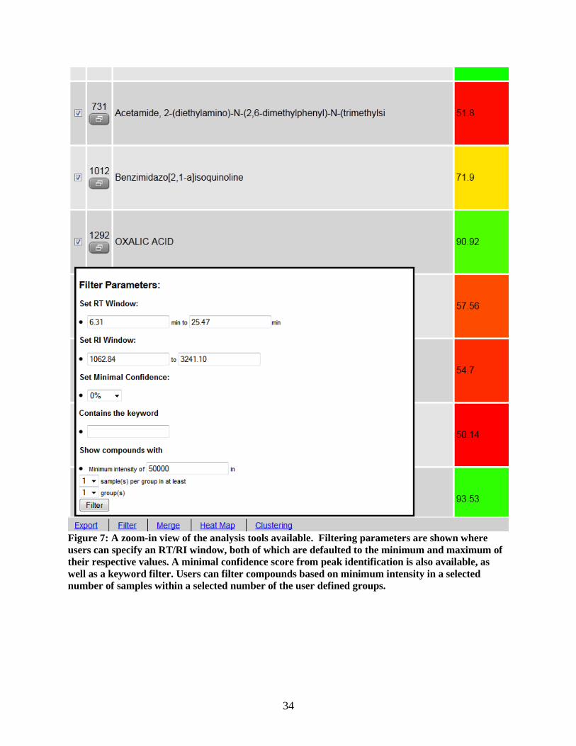
Filtering Function

A metabolite profiling experiment typically generates over 100 matched metabolite sets per

sample in the experiment. To facilitate manual data inspection or exploration, a “Filter” option is

provided in the toolbar to reduce the metabolite sets for onscreen display. Various filter parameters are

provided, such as keyword, minimum confidence, and RT/RI windows. . Semi-advanced filtering options

allow the user to filter metabolites based on their consistent detection (using a user-supplied cutoff) across

replicates or experimental groups. These options are designed to remove low-quality or spurious data,

and should be particularly helpful when used in conjunction with other statistical and visualization tools.

20

Statistical Analysis and Visualization

Heat maps are provided to allow a visually intuitive comparison of relative abundance amongst a

selected set of metabolites. Users are able to perform a heat map either by group or by ratio of selected

groups. Users must select candidate metabolite sets prior to generating a heat map. There is not a limit to

the number of metabolites that can be selected for heat map generation.

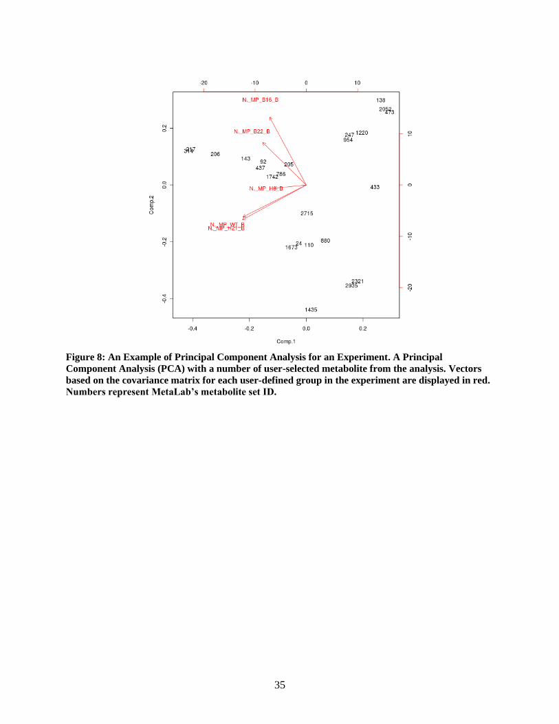
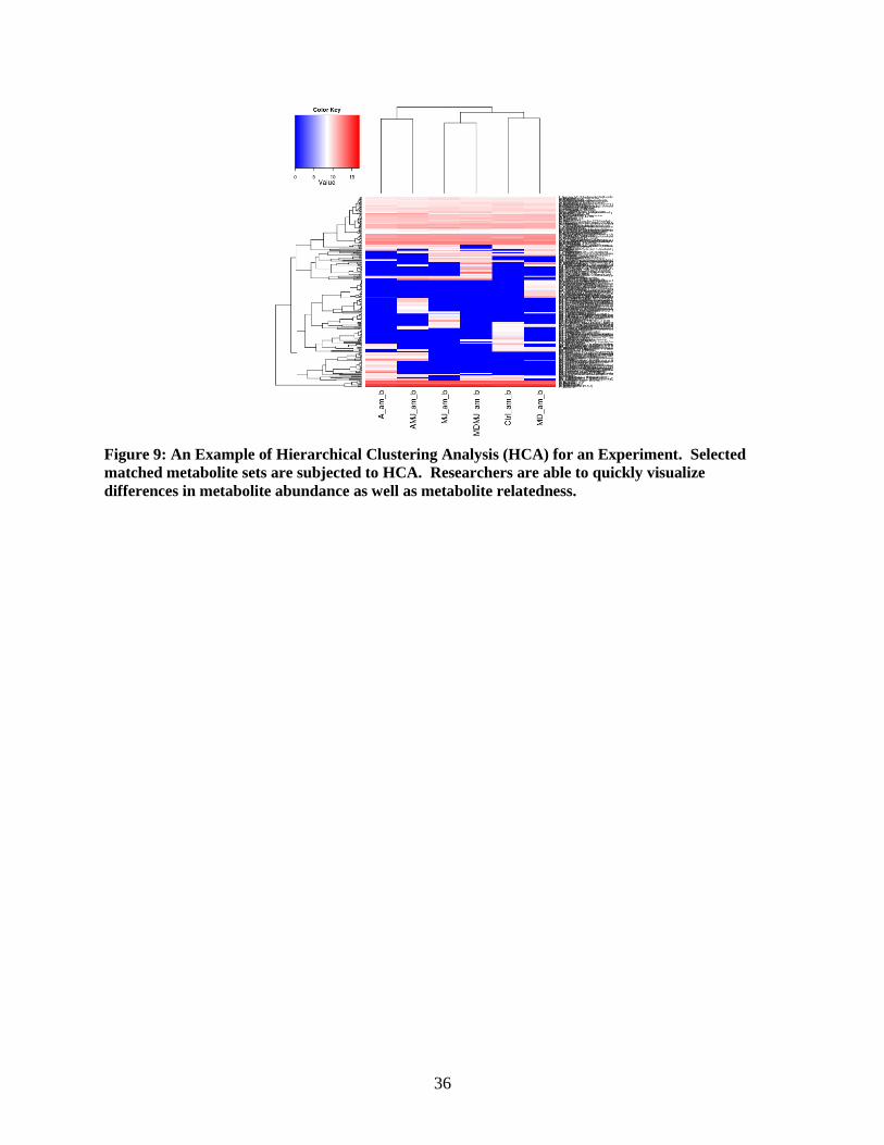
Two types of clustering options are currently available. Users can select metabolites of interest

from the summary page for Principal Component Analysis (PCA) or Hierarchal Clustering Analysis

(HCA). MetaLab implements these tools using the BioConductor R package (Gentleman et al. 2004).

The PCA function provides a visualization of the covariance matrix of the selected metabolites and

displays whether the metabolites are linearly related (Figure 8). The HCA provides a dendrogram display

of the selected metabolites, as well as the experimental groups, based on the complete linkage similarity

measure (Figure 9). The metabolite abundance information is also shown as a heat map. Below each

graphic display are options to export the image in Scalable Vector Graphic (SVG) or Encapsulated

PostScript (EPS) format. SVG graphics are vector-scalable (they do not lose resolution) and are ideal for

poster presentation, while the EPS format allows the user to break down the image and manipulate its

contents. Covariance or similarity matrixes used to generate the PCA or HCA graphs can also be

exported for other applications.

Data Export

The results of the experimental analysis can be exported to Excel® format for offline data mining

and analysis. This is performed by selecting the metabolite sets for export manually or by checking the

“Export All” checkbox at the top of the summary table. The user can customize the parameters to be

included, such as RT, RI, Raw Area, Normalized Area, Confidence, and Probability. MetaLab will export

the data to an Excel® spreadsheet in a format that is similar to the summary page display, with results

from different normalization methods populated into different sheets. The exported data will

21

automatically color-code each identified metabolite across samples within the experiment to facilitate

manual tracking.

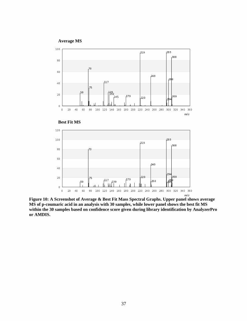
Metabolite Detail Reports

Users can view the details of a matched metabolite set by selecting the icon to the left of the

metabolite name in the summary table. This will display specifics pertaining to the metabolite set. A

graphical comparison of the Mass Spectral profile between the group average and the best fit individual

(metabolite with the highest reported confidence from library search) is displayed (Figure 10). Pseudo-

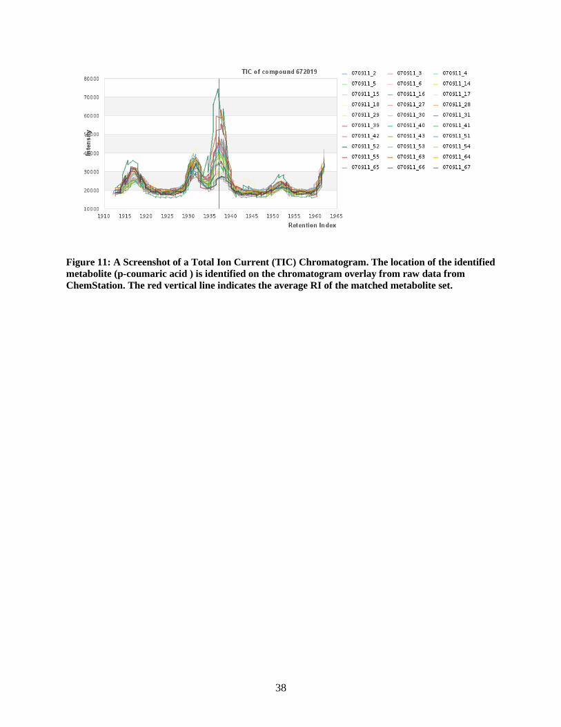
chromatogram overlaps across all samples for the given metabolite are shown in three different formats:

the raw chromatograms, and the TIC- and IS-normalized chromatograms (Figure 11). A display window

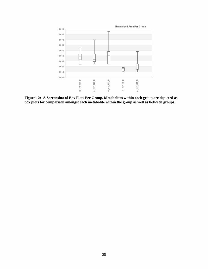
of ± 25 RI units is used, based on the raw MS data from the ChemStation. Metabolite abundance is

graphed in a box plot to present the data on a per group basis, using the specified normalization method

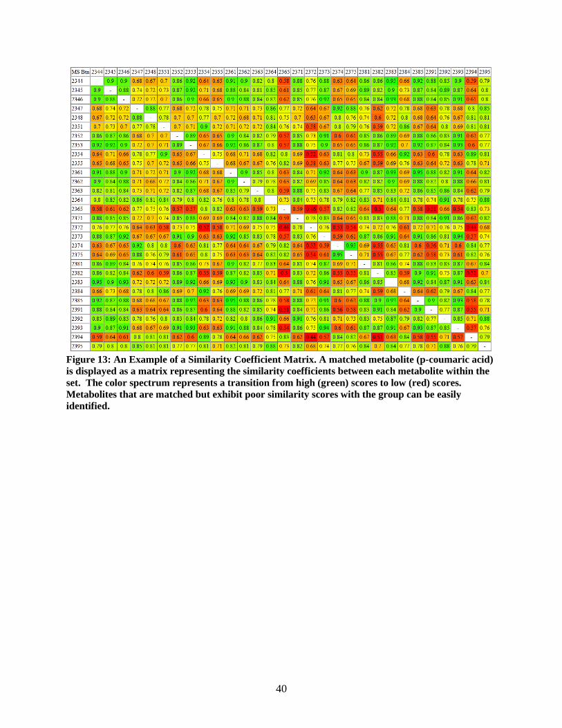
(Figure 12). The corresponding spectra similarity matrices used in peak-alignment is shown in a tabular

format by sample group, and in all-against-all color-coded matrices for the entire experiment or by sample

group (Figure 13). This allows users to quickly identify potential outliers as a quality control check.

Search Function

Metabolites can be queried for by using the Search Function feature of MetaLab. The lookup

feature performs a keyword search within both unanalyzed raw samples and matched metabolite sets.

Users can limit the search by various filters, such as RT/RI time windows, keywords on metabolite

names, researcher, pre-defined metabolic pathways or groups, or biological sample ID numbers.

Currently, there is one predefined pathway, Kreb‟s cycle, and one predefined group of metabolites, amino

acids. Additional metabolite groups or pathways can be added to the database by the system

administrator using the Database Administration tool.

22

Viewing Existing Experiments

All experiments are cataloged once generated. They can be viewed by selecting the “Open an

Existing Experiment” tab from the menu. Existing experiments can be browsed based on researcher,

experimental dates, and keywords.

Database Administration and User Authentication

MetaLab contains a backend administration panel for ease of database management.

Experimental factors such as new genotypes or tissue types can be added, updated, or deleted from a

backend interface rather than direct manipulation of the database itself through the command line.

Analysis progress can be checked by viewing any currently running experiment; if the runtime greatly

exceeds the estimated runtime, the faulty analysis can be identified and restarted by changing the status of

the analysis in the backend to IQ (in queue).

Administrators can also add GC-MS maintenance dates, such as column trimming and column

replacement. Maintenance data is important as it can be incorporated into sample data, and allow users a

mean to monitor and compare RT drift of the samples. It can also be used to identify any issues with

corrupted or erroneous outputs by comparing to other samples run on the GC-MS machine around the

same time.

A user hierarchy is implemented to assign roles between administrators, users, and a guest login.

Guests have access to view and search experiments performed by users, but do not have access to

experiment creation or editing. The user role inherits the permissions of the guest as well as having access

to upload samples, manage all aspects of experiment creation and analysis, and the ability to edit his or

her own experiment. Users do not have privilege to delete their created experiments. Administrators also

have access to sample, user, experiment and experimental factor management.

23

CHAPTER 4

DISCUSSION

The vast range of features in MetaLab has been designed with simplicity for the targeted end

user, the biologist, in mind. User feedback on possible system enhancements has driven the direction of

MetaLab to incorporate additional features, improved data handling, and overall enhanced user

experience. Such features begin at the point of data upload and range all the way to system

administration.

A web browser configuration provides a familiar environment to the user as well as the

portability of needing only an internet connection of a computer versus working around software

compatibility issues. Thus, system requirements to the end user are limited to the internet connection on

their particular computer, while the performance of MetaLab is based on the web server on which it is

installed.

Automated Features

MetaLab focuses on catering to the end user. MetaLab has attempted to automate as many steps,

as seamless as possible to reduce manual efforts, while providing various QC or editing features to help

users identify and correct errors. Prior to implementing the automated XML file fix, the researcher would

have to manually determine the source line of the error, and even using an XML validator, this process

could take up to an hour to correct all the data. As compared to manual curation, which has been noted to

take between five hours and a few days, a typical MetaLab experiment takes around twenty minutes to 3-

4 hours, depending on the number of samples and metabolites in the experiment. Much of this time is

devoted to peak matching, but there is still a significant saving in researcher time.

24

Many of the pages displayed in MetaLab are created dynamically. One example is the

experimental factor information, which is accessed across many different pages in MetaLab. By storing

the experimental factor information in the database, it can be accessed and displayed without the

administrator having to update several different files when a new factor is added to the database. For

example, an experimental factor template file is created dynamically based on experimental factors stored

in the database marked as active. These factors are also displayed on forms when new sample data is

uploaded. As new experimental factors are added to the database and marked as active, the experimental

factor template file will be automatically updated to reflect the new entries and available to users for data

upload.

Analysis and Data Display Features

MetaLab strives to provide a biologist-friendly platform for metabolite profiling data analysis,

exploration and display. Upon experiment completion, the user is presented with a substantial amount of

data on the summary page. From here, the researcher can identify differences in average peak areas and

their respective standard deviations for the user-specified groups. The user can sort by average SC to

determine which metabolites grouped together the best, or the user can sort on p-value to view the most

significantly changed metabolites within the experiment. Connecting all of the features on the analysis

summary page is a useful toolbar that remains in fixed position at the bottom of the browser screen.

Implementation of this feature is driven by interactive popup menus that allow various tasks to be

performed on selected matched sets, such as filtering options, merging of matched sets, and various other

statistical tools including heat maps and PCA and HCA clustering. Metabolite abundance across

experimental groups can be easily visualized using heat maps, and metabolite sets that are statistically

similar would be apparent using PCA and HCA clustering.

From the analysis summary page, users are able to explore the individual metabolites by clicking

the image to the left of the entry. Intuitive information such as the spectral similarity matrix allows the

researcher to view the underlying matching pattern of the set and perhaps identify problematic

25

metabolites within the matched set. Users can also explore raw data extracted from the original data files.

The ability to view raw data is helpful when unexpected results occur, and this information can help

indicate the source of the problem, whether it be problem of raw data or misalignment by MetaLab.

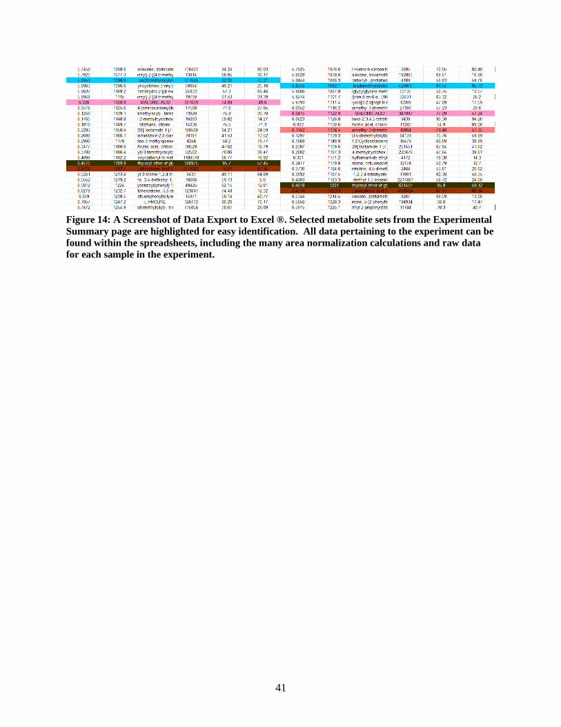
One of the most useful features in MetaLab is the ability to export the results of an analysis,

complete with automated color-coding of matching metabolites across samples (Figure 14). Manual

curation of this type of compound identification has been reduced from what could take several hours to

minutes, while keeping if not improving accuracy. MetaLab exports all analysis results as seen on-screen

to a multi-sheet Excel format. By exporting experimental data, users are no longer limited to data

manipulation within MetaLab. Data can be analyzed off-line using other more sophisticated statistical

tools.

System Management

MetaLab has a user interface to provide researchers as well as administrators with tools to

monitoring instrument performance for quality control. The user access panel initially warns users of files

that are missing important markers relevant to creating an analysis. Graphs depicting retention time

markers over time also indicate GC maintenance dates, which can be taken into account during

experiment/data troubleshooting. Graphs also indicate the identified internal standards over the lifetime

of inserted data, depicting retention time fluctuations and corresponding retention index calculations.

Calculated retention index scores are flagged for user review when the internal standard retention index

deviates beyond a certain percentage, 1% by default, of the average. This allows the user to easily

identify misidentified retention markers within the system. Users are able to edit markers within each of

their samples accordingly from the user access panel.

System administrator has the privilege to edit or delete any user data from a graphical interface

without affecting the integrity of the backend. Editing the backend manually is tedious and prone to

errors. Much of the system can be edited by using a user interface in order to maintain this integrity.

26

Data Optimization

The original MetaLab prototype did not incorporate a true relational database style. Upload of

roughly 200 samples with corresponding data consumed roughly 1.2GB of data storage. MetaLab

effectively reduced this demand by incorporating data optimization techniques to split and optimize data

tables. The result of the design changes was a 75% gain in storage efficiency.

Future Improvements

MetaLab‟s relational database design means that many future improvements can be easily

implemented to increase its versatility and value for the end user. Regular maintenance should focus on

keeping the system up-to-date with compatibility of feature and software improvements. Rapid

development of open source technologies on which MetaLab is built will require minor code changes to

keep MetaLab working efficiently. The incorporation of frameworks, such as PHPExcel and the release

of new versions of Microsoft Excel® have already given rise to updated pipelines.

One of the main bottlenecks in the current implementation lies with the types of file formats

accepted, limiting to AnalyzerPro and AMDIS. By accepting more popular input file types, MetaLab can

expand to serve a wider range of users. Accepting new input files would require new code to handle the

specific file types.

Improvements to database insertion queries with advances in database technology have given rise

to new, more efficient ways of database insertion. MySQLi and the recent addition of PHP Data Objects

(PDO) drastically reduce query insertion, deletion and update times when dealing with large data sets.

Such improvements should be incorporated in the future. In addition, utilization of a multi-threaded

capable programming language, such as C++, to calculate and store similarity coefficient scores to the

database would greatly improve the speed of analysis.

27

CHAPTER 5

CONCLUSION

We have presented MetaLab as a user-friendly, web-based portal for GC-MS-based metabolite

profiling data processing and analysis. The current system houses over 2500 samples and nearly 225 GC-

MS experiments. Considering that a variety of GC-MS data deconvolution and peak identification

software packages, both commercial and open-source, are already available, MetaLab does not attempt to

duplicate these efforts. Instead, MetaLab uses both raw GC-MS data files (such as those generated by

Agilent ChemStation) and deconvoluted data files (such as those from AnalyzerPro and AMDIS) as the

starting point. Although the current release is designed for GC-MS data, the system can be modified to

accept and analyze LC-MS data. Most of the tools in place are extensible to LC-MS data. The two

compatible metabolite deconvolution and identification software packages, AnalyzerPro and AMDIS, are

able to accept LC-MS as input data as well.

MetaLab‟s user interface allows researchers to easily categorize their experiments and output the

results for further use. MetaLab is designed to streamline the tedious data analysis process by automating

peak matching and identifying matches across deconvoluted data that may well present contrasting library

names across samples. Data that has been analyzed can easily be exported and reorganized. What may

have taken a researcher days to achieve manually can be completed in MetaLab in a fraction of the time.

MetaLab therefore allows the researchers to focus their time and effort on the biological interpretation of

the metabolite profiling results. Guest access to view data and experiments is available via web access at

http://aspendb.uga.edu/metalab.

28

Figure 1: An example of GC-MS results. The chromatogram (top) indicating the elution time and

intensity of detected metabolites. The mass spectrum (bottom) shows the mass fragmentation

pattern corresponding to the peak at 8.27 min.

29

Figure 2: An example of the folder structure required for sample submission. Both AnalyzerPro

and AMDIS samples require the ChemStation data folder containing the CHROMTAB.CSV file.

MetaLab will automatically identify samples as an AnalyzerPro results file or AMDIS results file.

30

Figure 3: The graphical depiction of retention time (RT) versus retention index (RI) for the

Internal Standard (IS) Adonitol. Column maintenance and experimental factors cause shifts in

retention time over the course of the column lifespan. Retention time values are shown in red

squares and green triangles, representing samples analyzed before and after a GC column

replacement event (red line), respectively. Retention Index remains relatively unchanged over the

course of a column replacement (blue diamonds).

31

Figure 4: MetaLab's Relational Database Concept. The groups of tables listed are relationally

linked in order to conserve space and optimize querying time by utilizing indices (keys).

32

Figure 5: A Screenshot View of MetaLab Sample Submission. The MetaLab upload page provides a

CSV download of all experimental factors contained in the database. An optional Comma

Separated Value (CSV) formatted file named “sample.csv” can be included to automate

experimental factor selection for samples within the container ZIP file. This file can be validated

using the Factor Format Validator.

33

Figure 6: A Screenshot View of Experimental Results. Experiment information and samples within

each user-defined group are displayed at the top. Each row represents a matched metabolite set.

Names of the metabolite with the highest confidence within the set are displayed, or if a common

name is available, it is displayed in green. Confidence displays the confidence score of the

metabolite highest confidence within the matched set. RI and RT represent the average RI and RT

values for the matched set. P-Val and Q-Val represent the statistical significance of the metabolite

set based on ANOVA and SLIM (Wang et al. 2011). Each column can be sorted by clicking the

column heading. Various normalization calculations can be displayed for each group based on

selection of normalization method.

34

Figure 7: A zoom-in view of the analysis tools available. Filtering parameters are shown where

users can specify an RT/RI window, both of which are defaulted to the minimum and maximum of

their respective values. A minimal confidence score from peak identification is also available, as

well as a keyword filter. Users can filter compounds based on minimum intensity in a selected

number of samples within a selected number of the user defined groups.

35

Figure 8: An Example of Principal Component Analysis for an Experiment. A Principal

Component Analysis (PCA) with a number of user-selected metabolite from the analysis. Vectors

based on the covariance matrix for each user-defined group in the experiment are displayed in red.

Numbers represent MetaLab’s metabolite set ID.

36

Figure 9: An Example of Hierarchical Clustering Analysis (HCA) for an Experiment. Selected

matched metabolite sets are subjected to HCA. Researchers are able to quickly visualize

differences in metabolite abundance as well as metabolite relatedness.

37

Average MS

Best Fit MS

Figure 10: A Screenshot of Average & Best Fit Mass Spectral Graphs. Upper panel shows average

MS of p-coumaric acid in an analysis with 30 samples, while lower panel shows the best fit MS

within the 30 samples based on confidence score given during library identification by AnalyzerPro

or AMDIS.

38

Figure 11: A Screenshot of a Total Ion Current (TIC) Chromatogram. The location of the identified

metabolite (p-coumaric acid ) is identified on the chromatogram overlay from raw data from

ChemStation. The red vertical line indicates the average RI of the matched metabolite set.

39

Figure 12: A Screenshot of Box Plots Per Group. Metabolites within each group are depicted as

box plots for comparison amongst each metabolite within the group as well as between groups.

40

Figure 13: An Example of a Similarity Coefficient Matrix. A matched metabolite (p-coumaric acid)

is displayed as a matrix representing the similarity coefficients between each metabolite within the

set. The color spectrum represents a transition from high (green) scores to low (red) scores.

Metabolites that are matched but exhibit poor similarity scores with the group can be easily

identified.

41

Figure 14: A Screenshot of Data Export to Excel ®. Selected metabolite sets from the Experimental

Summary page are highlighted for easy identification. All data pertaining to the experiment can be

found within the spreadsheets, including the many area normalization calculations and raw data

for each sample in the experiment.

42

REFERENCES

Babushok VI, Linstrom PJ, Reed JJ, Zenkevich IG, Brown RL, Mallard WG, Stein SE (2007) Development of

a database of gas chromatographic retention properties of organic compounds. Journal of

Chromatography A 1157: 414-421

Bino RJ, Hall RD, Fiehn O, Kopka J, Saito K, Draper J, Nikolau BJ, Mendes P, Roessner-Tunali U, Beale MH,

Trethewey RN, Lange BM, Wurtele ES, Sumner LW (2004) Potential of metabolomics as a functional

genomics tool. Trends in Plant Science 9: 418-425

Colinet H, Renault D, Charoy-Guével B, Com E (2012) Metabolic and Proteomic Profiling of Diapause in

the Aphid Parasitoid <italic>Praon volucre</italic>. PLoS ONE 7: e32606

Davies AN (1998) The new Automated Mass

Spectrometry Deconvolution and

Identification System (AMDIS). Spectroscopy Europe 10: 4

Dunn WB, Ellis DI (2005) Metabolomics: Current analytical platforms and methodologies. TrAC Trends in

Analytical Chemistry 24: 285-294

Ettre LS (1993) NOMENCLATURE FOR CHROMATOGRAPHY. Pure Appl. Chem. 65: 819-872

Ferry-Dumazet H, Gil L, Deborde C, Moing A, Bernillon S, Rolin D, Nikolski M, de Daruvar A, Jacob D

(2011) MeRy-B: a web knowledgebase for the storage, visualization, analysis and annotation of plant

NMR metabolomic profiles. BMC plant biology 11: 104

Fiehn O (2002) Metabolomics – the link between genotypes and phenotypes. Plant Molecular Biology

48: 155-171

43

Gentleman RC, Carey VJ, Bates DM, Bolstad B, Dettling M, Dudoit S, Ellis B, Gautier L, Ge Y, Gentry J,

Hornik K, Hothorn T, Huber W, Iacus S, Irizarry R, Leisch F, Li C, Maechler M, Rossini AJ, Sawitzki G, Smith

C, Smyth G, Tierney L, Yang JY, Zhang J (2004) Bioconductor: open software development for

computational biology and bioinformatics. Genome biology 5: R80

Haerder T, Reuter A (1983) Principles of transaction-oriented database recovery. ACM Comput. Surv. 15:

287-317

Karp PD, Ouzounis CA, Moore-Kochlacs C, Goldovsky L, Kaipa P, Ahrén D, Tsoka S, Darzentas N, Kunin V,

López-Bigas N Expansion of the BioCyc collection of pathway/genome databases to 160 genomes.

Nucleic Acids Research 33: 6083-6089

Kastenmuller G, Romisch-Margl W, Wagele B, Altmaier E, Suhre K (2011) metaP-server: a web-based

metabolomics data analysis tool. Journal of biomedicine & biotechnology 2011

Kind T, Wohlgemuth G, Lee DY, Lu Y, Palazoglu M, Shahbaz S, Fiehn O (2009) FiehnLib: Mass Spectral and

Retention Index Libraries for Metabolomics Based on Quadrupole and Time-of-Flight Gas

Chromatography/Mass Spectrometry. Analytical Chemistry 81: 10038-10048

Lam H, Deutsch EW, Eddes JS, Eng JK, King N, Stein SE, Aebersold R (2007) Development and validation

of a spectral library searching method for peptide identification from MS/MS. PROTEOMICS 7: 655-667

Lu H, Liang Y, Dunn WB, Shen H, Kell DB (2008) Comparative evaluation of software for deconvolution of

metabolomics data based on GC-TOF-MS. TrAC Trends in Analytical Chemistry 27: 215-227

Neuweger H, Albaum SP, Dondrup M, Persicke M, Watt T, Niehaus K, Stoye J, Goesmann A (2008)

MeltDB: a software platform for the analysis and integration of metabolomics experiment data.

Bioinformatics 24: 2726-2732

Project TP (2009) PubChem.

Rasmussen S, Parsons AJ, Jones CS (2012) Metabolomics of forage plants: a review. Annals of Botany

44

Smyth GK, Michaud J, Scott HS (2004) Use of within-array replicate spots for assessing differential

expression in microarray experiments. Bioinformatics 21: 2067-2075

Stein S, Scott D (1994) Optimization and testing of mass spectral library search algorithms for compound

identification. Journal of the American Society for Mass Spectrometry 5: 859-866

Stein SE (1999) An integrated method for spectrum extraction and compound identification from gas

chromatography/mass spectrometry data. Journal of the American Society for Mass Spectrometry 10:

770-781

Wang H-Q, Tuominen LK, Tsai C-J (2011) SLIM: a sliding linear model for estimating the proportion of

true null hypotheses in datasets with dependence structures. Bioinformatics 27: 225-231

Xia J, Psychogios N, Young N, Wishart DS (2009) MetaboAnalyst: a web server for metabolomic data

analysis and interpretation. Nucleic Acids Research 37: W652-W660