Embed Size (px)
Citation preview
CONFIDENTIAL
Oakland University Final February 2008
Page 1 of 55
Meteorological Tower Data
Compilation and Analysis
Oakland University
February 19, 2008
Prepared for
Terry Stollsteimer, Assoc. VP for Facilities Management
James F. Tallman, Director of Engineering
James A. Leidel, Energy Manager
Prepared by
ALTERNATE ENERGY SOLUTIONS, INC.
23801 Gratiot Ave.
Eastpointe, MI 48021
Telephone (586) 498-8840
Facsimile (586) 498-8858
Member: American Council of Renewable Energy (ACORE)
National Wind Coordinating Committee (NWCC)

CONFIDENTIAL
Oakland University Final February 2008
Page 2 of 55
Preface _________________________________________________________________________________________________________________________________________________________________________________________________________________________________________________
This document has been prepared by Alternate Energy Solutions, Inc. and presents essential points of
discussion pertaining to the study of wind resource at Oakland University. The study was commissioned by
Mr. James Leidel, Energy Manager for Oakland University, in late 2005.
We anticipate this document will serve to enlighten and educate the reader on matters pertaining to the
history of this undertaking, wind and wind power, the local wind regime, wind turbine energy capture, and
topics considered relevant to project development.

CONFIDENTIAL
Oakland University Final February 2008
Page 3 of 55
Table of Contents _________________________________________________________________________________________________________________________________________________________________________________________________________________________________________________
Executive Summary ……………………………………………………………………………… 4
1. Introduction …………………………………………………………………………... 5
2. Methodology …………………………………………………………………………. 7
3. Wind and Measurement ……………………………………………………………… 12
4. Factors Affecting Wind Power and Turbine Performance …………………………… 20
5. Data Validation and Reporting ……………………………………………………….. 30
6. Collected Wind Data ...……………………………………………………………….. 32
7. Historical Wind Data, Correlation and Prediction……………………………………. 49
8. Wind Turbine Availability and First Energy Capture Estimate ..…………………….. 53
9. Recommendations ……………………………………………………………………. 55

CONFIDENTIAL
Oakland University Final February 2008
Page 4 of 55
Executive Summary _________________________________________________________________________________________________________________________________________________________________________________________________________________________________________________
The Oakland University Wind Study has found the wind regime to be suitable for on-site wind turbine
development using generators specifically designed for lower wind regimes. Tower hub heights equal to or
greater than 75m (246 ft) will be required for any meaningful conversion of wind energy. Due to many wind
flow obstructions in the near vicinity of the meteorological tower during the monitoring period, high wind
shear and roughness factors were recorded between 30m, 40m, and 50m sensor heights.
Several wind turbine generator models have been initially selected for closer review and analysis.
Nameplates ranged from 900kW to 2,000kW. Manufacturers and respective models have been grouped into
two tiers. Tier One is made up of wind turbines that are available and would present little difficulty to
acquire. Manufacturers making the first selection tier include: AAER 1500-77; AWE 54-900; Enercon E82;
and Fuhrlander FL1500. Tier Two consists of wind turbines meeting the selection criteria but may have
extended acquisition times, require a tower modification, or the manufacturer may not have responded to the
recent RFQ in a timely manner. Turbines that we have included into the second tier include: AWE 54-900;
Nordex S77; and Vestas V100.
Preliminary estimates for capacity factor on the first three units listed above range between 15.3% and 25.5%
We have assigned a tolerance of ±25% to the energy capture estimates. Equipment availability for the latter
two units has not been confirmed at the time of document printing. The significant local wind shear warrants
the investigation of upper level physics, to further validate wind velocities and energy capture calculations.
Recommendations for Computational Fluid Dynamic (CFD) software modeling and/or Doppler sonar
investigations are strongly suggested.

CONFIDENTIAL
Oakland University Final February 2008
Page 5 of 55
Section 1
Introduction _________________________________________________________________________________________________________________________________________________________________________________________________________________________________________________
Alternate Energy Solutions initially met with Mr. James Leidel to discuss the possibility of developing one or
more on-site wind turbine generating facilities to offset the electrical energy demand of Oakland University’s
main campus. A Wind Tower Lease and Report Proposal was submitted by Alternate Energy Solutions, Inc.
for consideration on December 20, 2005, and accepted thereafter with an attached Memorandum of
Understanding. A meteorological tower was assembled and erected during the month of February, 2005, for
the purpose of monitoring and recording wind conditions on campus. Monitoring and recording commenced
February 21, 2006. The meteorological tower was leased to Oakland University for a period of one year
under the agreement, and the lease was subsequently extended for a second one-year period. The extension
of the second lease period will end on February 20, 2008, at which time the meteorological tower will be
disassembled and removed from campus. This document is being completed prior to the completion of the
second year of data gathering and includes data recorded through December 31, 2008.
After mutual review of the wind data recorded from the first year of monitoring and careful consideration of
wind turbine equipment designed for lower wind speed regimes, it was determined that an added
investigation into wind turbine generation was merited. Wind data collected at Oakland and information in
this document, derived from the collected data, is jointly owned by Oakland University and Alternate Energy
Solutions, Inc.
On April 9, 2007, Alternate Energy Solutions, Inc. (“AESI”) submitted a Wind Generation Feasibility Study
Proposal under the request of Oakland University (“Oakland”). The Proposal was accepted on July 26, 2007.
Under the terms of the feasibility study, AESI was to review possible locations for wind development and
evaluate each location’s comparative cost for proposed wind turbine generators ranging from 900 kW to
2,000 kW.
Factors which were considered by Facilities Management personnel and AESI in selecting a test site for the
installation of the meteorological tower included, but not limited to:
• The amount for open area that could be devoted to wind project development
• Ground cover, forest areas, and existing obstructions to wind flow
• Proximity and accessibility to distribution and transmission lines
• Logistics for heavy construction equipment staging and year-round access to the site

CONFIDENTIAL
Oakland University Final February 2008
Page 6 of 55
After careful review, the decision was made with Facilities Management to place one 50m meteorological
tower in an open field west of the Detroit Edison Spencer Substation located on university property. The
substation is located south of Lonedale Rd. and east of Squirrel Rd.
Map of Oakland University and Meteorological Tower Installation Courtesy DeLorme Topographic Maps

CONFIDENTIAL
Oakland University Final February 2008
Page 7 of 55
Section 2
Methodology and Principles _________________________________________________________________________________________________________________________________________________________________________________________________________________________________________________
Methodology is traditionally defined as the analysis of, development of, or a given set of procedures that are
applied within a disciplined study. Methodology, as it is applied in the analysis of a wind regime and
incorporated by this white paper, includes the following concepts as they relate to wind energy.
• Collection and Research
• Development of Data Validation
• Data Validation
• Treatment of Suspect or Missing Data
• Analysis of Data
This report has been compiled using the wind energy resource assessment handbook for industry accepted
guidelines, modeled under the Utility Wind Assessment Program (UWRAP), and developed by the U.S.
Department of Energy (USDoE) in 1995. UWRAP was commissioned by the USDoE and further
administered by the Utility Wind Interest Group having as its mandate the technical support for utilities that
conduct assessment of wind regimes.
Sophisticated proprietary software, under license to Alternate Energy Solutions and specifically designed for
wind energy analysis, was utilized in the preparation of this white paper. The recommendations from learned
engineers and meteorologists having experience with wind energy through collaboration with the National
Renewable Energy Laboratories (NREL/USDoE) and the National Weather Service (NWS/USDoC) were
consulted.
Collection and Research
This study involved researching available wind data sources and wind mapping programs commissioned by
the State of Michigan Energy Office and Michigan Wind Working Group supported by the Michigan Public
Service Commission. International data sources were referenced for this undertaking. These sources included
the Canadian Wind Atlas and the Ontario Wind Resource Atlas to support monitoring the wind regime at
Oakland University.

CONFIDENTIAL
Oakland University Final February 2008
Page 8 of 55
Historical wind velocity data was compiled from three regional airports, namely Pontiac, Flint and
Detroit Metropolitan, for the purpose of comparing annual wind velocities to baseline data obtained
at Oakland.
Development of Data Validation
The validation of collected data was performed using manual inspection and computer-based software,
sampling collected raw data files against recorded weather data from sources believed to be accurate. All
data files were checked each time they were collected.
There are many possible causes of erroneous data; hence, some attention is now given in the white paper to
foster awareness for the benefit of the reader. During the course of the data monitoring process several
events may lead to erroneous data being recorded.
Possible causes for erroneous data records include the following situations:
• Faulty or Damaged Sensors
• Loose Wire Connections
• Broken Wires and Damaged Instrument Cables
• Damaged Mounting Hardware
• Faulty or Damaged Power Supply
• Data Logger Malfunctions
• Static Discharge
• Lightning Discharge
• Icing Conditions
• Birds Perched or Nesting on Instrument Booms
Data Validation
The primary objective of data validation is to detect as many significant errors and their reasons as possible.
The significant errors are generally quite easily recognized; however, it is the subtle errors, hard to detect,
that are discovered by a fastidious and meticulous investigation of the data prior to processing.

CONFIDENTIAL
Oakland University Final February 2008
Page 9 of 55
An example would be that of sensor connectivity to the data logger. In the case of a sensor wire that is
broken or disconnected, data for the affected channel would tend to be recorded at an extreme and constant
value. This type of malfunction would be readily apparent in the data records. However, under the condition
of a sensor wire that is connected to a screw terminal point where the contact is intermittent, because the
screw may have become loosened (due to tower wind vibration, temperature change, or outside force acting
upon the wire or cable). This would cause the data for the affected channel to blend-in with the other data
records and its erroneous nature would not be as apparent. Therefore, these slight deviations in the data can
escape detection, but by incorporating redundant sensors this possibility is reduced.
To facilitate data validation, several routines are designed and utilized to screen the measured parameters for
possible errors. These routines may be best categorized as tests on the general system and tests on the
measured parameters.
1. General System Checks:
Basic tests to evaluate the completeness of the site data collected:
• Data Records: Counting the number of data files and records that were
recorded by the logger, and comparing to the expected number of data files and
records for the time period that recording was being performed.
• Time Sequence: Review of the time and date stamp on each data record to determine
if there are missing sequential data files and records.
2. Measured Parameter Checks:
• Range Tests: Measure data is compared to upper and lower threshold values.
• Rational Tests: Comparison of physical relationship between sensor parameters.
• Trend Tests: Evaluating the rate of change in data values over a period of time.
Treatment of Suspected or Missing Data

CONFIDENTIAL
Oakland University Final February 2008
Page 10 of 55
Generally, in the case of missing or suspect data, a flag is placed on the data set and affected channel prior to
analysis. Based on the amount and significance of the data that is suspect with respect to the particular
calculations that it is being used for, a decision to omit suspect data is rendered.
There are essentially two components to data validation:
a) data screening
b) data verification.
Data screening is performed manually and by use of validation routines or algorithms to screen all data for
suspect values, those which appear questionable or erroneous. If a data value is suspect, it is not necessarily
in error. The suspect data is then scrutinized on a case-by-case basis and a decision is made on how to best
handle the data.
This decision, made with scrutiny, will result in one of the following actions:
a) retain data as valid;
b) reject data as invalid;
c) replace data with valid correlated values;
d) replace with average values; or
e) replace data with synthesized values using special algorithms.
Analysis of Data
After the data has been validated, the data is subjected to processing procedures to evaluate the wind
resource. The processing typically involves many calculations and the sorting of data into useful subsets.
The hourly averages for the collected data are traditionally used for reporting purposes. This is accomplished
by combining validated 10-minute data averaged subsets into an hourly average. In this part of the process,
flagged data (erroneous) that has been rejected must not inadvertently be used in the calculations.

CONFIDENTIAL
Oakland University Final February 2008
Page 11 of 55
Calculations that were recommended and performed during the analysis of data include:
• Average wind velocity
• Probability Distribution Function, Weibull distribution ‘k’ factor and ‘c’ factor
• Temporal variations (diurnal, weekly, monthly, annually)
• Cumulative Distribution Function (Inverse Integration of Distribution Function)
• Anemometer shading
• Wind Speed Profiles
• Determination of vertical wind shear exponent and wind shear profile
• Turbulence intensity
• Air density
• Wind power density
• Rose diagrams
• Wind energy capture estimate

CONFIDENTIAL
Oakland University Final February 2008
Page 12 of 55
Section 3
Wind and Measurement _________________________________________________________________________________________________________________________________________________________________________________________________________________________________________________
Regional Nature of Wind
Winds are classified traditionally as either general or local. General wind circulation may stretch thousands
of miles over the surface of the planet. These winds have what are referred to as semi-permanent directional
patterns near the surface and extending into the atmosphere. Local winds are superimposed on the general
wind currents, e.g., a thunderstorm in the summer or winter squall.
The primary determining factor in general wind circulation patterns is the unequal heating of the atmosphere
and surface at different elevations and latitudes. The rotation of the earth’s rotation is also a subtle
contributing factor in general circulations. The distribution of atmospheric pressure is closely related to
general wind development.
Development of Wind Patterns between High and Low Pressure Systems
General wind circulations are categorized into seven regions along the various latitudes of the earth’s surface.
• North Polar Easterlies
• North Hemisphere Westerlies
• Northeast Trades
• Doldrums
• Southeast Trades
• South Hemisphere Westerlies
• South Polar Easterlies
Wind Vectors, Water Temperature and Ice Levels
from Earth System Grid (ESG) Courtesy National Center for Atmospheric Research (NCAR)
CONFIDENTIAL
Oakland University Final February 2008
Page 13 of 55
The Great Lakes region is largely influenced by the North Hemisphere Westerlies from the macro-weather
systems with sea-land breezes adding their effect to local wind conditions.
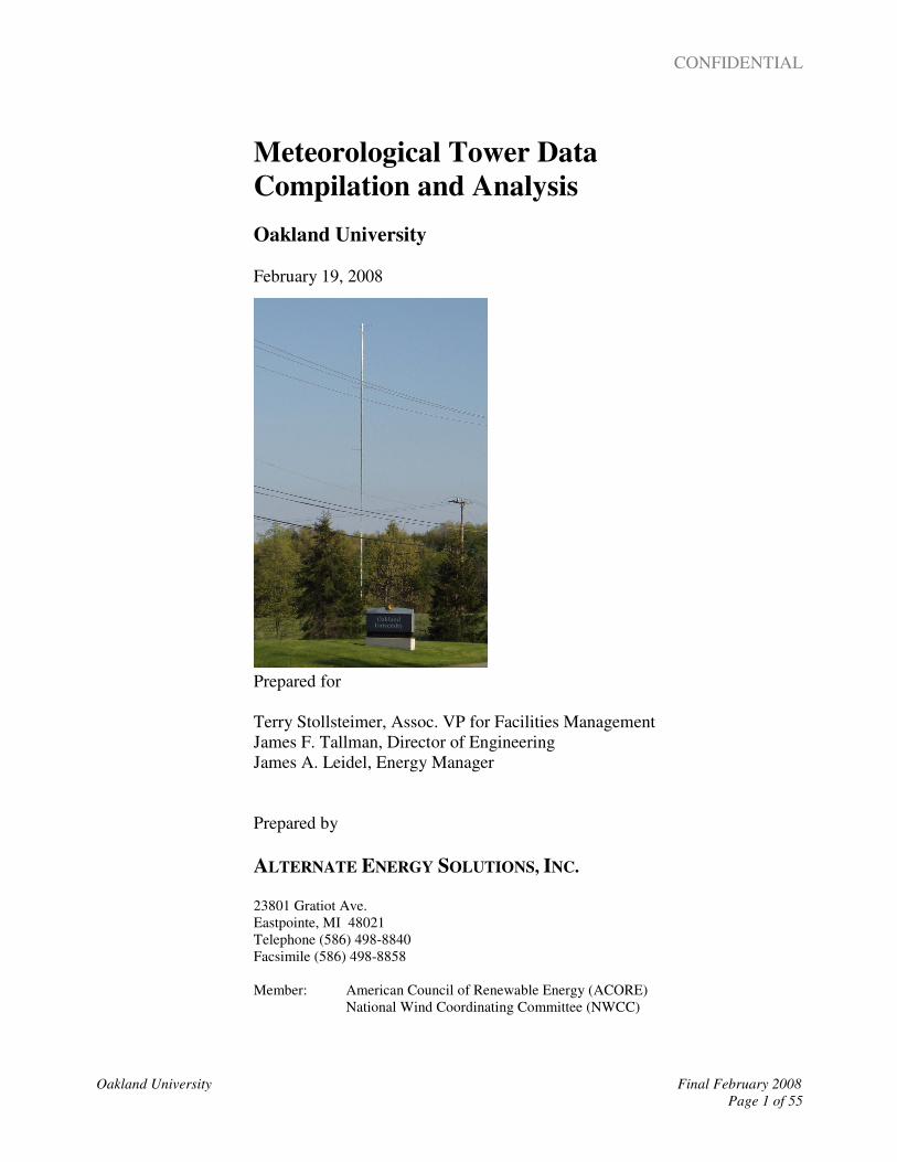
Sea-land breeze results from temperature gradients (differences of temperature) between coastal land and
adjacent bodies of water, namely, Lake St. Clair and Lake Huron. As the sun begins to shine and heat the
surface, the temperature of the land increases faster than that of the lake. This is because the lake is a heat
sink, having a lower coefficient of thermal resistance, which tends to maintain a more constant temperature.
Conversely, the land tends to have a higher temperature coefficient of resistance and therefore heats up faster
than the water. As the day progresses, the difference in temperature between the lake and land increases, the
warm air over the land rises, causing a lower pressure region over the land, which pulls the cooler air volume
from over the lake inland.
Conditions for Lake Breeze Effect
Direction Lake to Land Circulation
Highlighted Temperature Gradient for Daylight Warming Hours
CONFIDENTIAL
Oakland University Final February 2008
Page 14 of 55
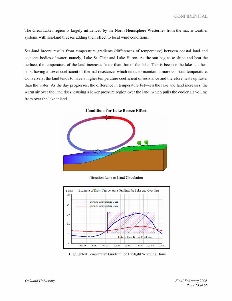
Toward the evening hours of the day, the temperature of the lake increases and the temperature of the land
begins to fall. The difference in temperature gradient between the two lessens; the land-sea breeze lessens,
until such time that the temperature gradient is zero. At this time there is no difference between the land and
the lake. Any wind due to the sea-land breeze effect will cease.
As evening passes to nightfall, the temperature over the land will tend to decrease, and the land temperature
will be below that of the lake. Again, a temperature gradient will form between the two, the lake having the
larger heat mass will cause air over the lake to rise and the cooler air over the land mass will be drawn out
over the lake.
Conditions for Land Breeze Effect
Direction Land to Lake Circulation
Highlighted Temperature Gradient Nightfall to Dawn Cooling Hours
CONFIDENTIAL
Oakland University Final February 2008
Page 15 of 55
SUNRISE SUNSET
Win
d V
elo
city
(kt)
150 ft
Time of Day
40 Feet
1500 ft
300 ft
600 ft
Generally, with smaller bodies of water, twice each day there will be point in time when the temperature of
the land mass and that of the lake mass will cross and be equal to one another. This condition marks the
beginning of a reversing circulatory cycle and direction of the air flow between the lake and the adjacent
coastal land. The amount of sea-land breeze that is developed varies with: seasonal factors, land mass,
vegetation and cover, and the heat mass of the body of water and currents.
The wind regime at Oakland is more so affected by macro-weather systems and to a lesser extent influenced
by the micro-weather systems of Lake St. Clair and Lake Huron.
The data measured at Oakland tends to suggest an Atmospheric Boundary Layer (ABL) wind effect. The
ABL is a layer of air having variable depth and is next to the ground cover of the earth. The ABL is generally
defined by the height to which the friction of earth’s ground cover, and to some degree terrain, act to lower
or retard wind velocity in those areas where heat exchange with the ground produces significant interaction
with one another. The depth of the ABL typically varies between 1,000 ft to 2,000 ft above ground level. One
of the most basic indicators of ABL wind effect is seen by near surface wind velocity pattern change during
sunrise and sunset transition periods.
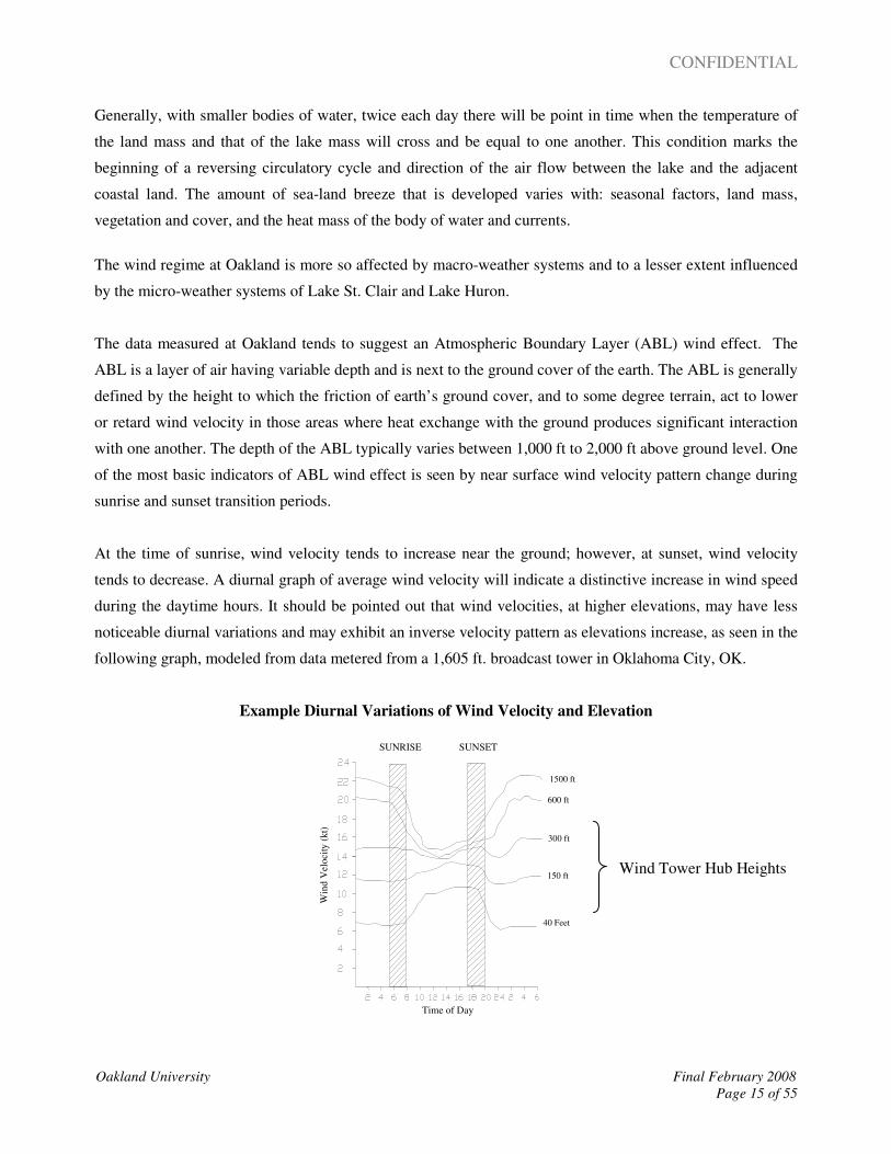
At the time of sunrise, wind velocity tends to increase near the ground; however, at sunset, wind velocity
tends to decrease. A diurnal graph of average wind velocity will indicate a distinctive increase in wind speed
during the daytime hours. It should be pointed out that wind velocities, at higher elevations, may have less
noticeable diurnal variations and may exhibit an inverse velocity pattern as elevations increase, as seen in the
following graph, modeled from data metered from a 1,605 ft. broadcast tower in Oklahoma City, OK.
Example Diurnal Variations of Wind Velocity and Elevation
Wind Tower Hub Heights
CONFIDENTIAL
Oakland University Final February 2008
Page 16 of 55
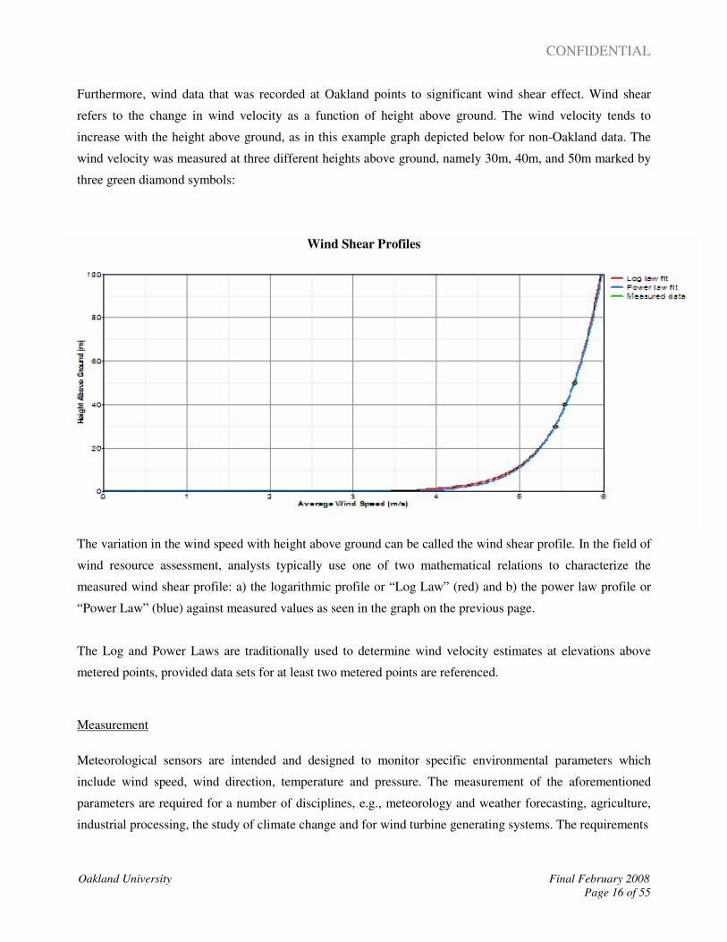
Furthermore, wind data that was recorded at Oakland points to significant wind shear effect. Wind shear
refers to the change in wind velocity as a function of height above ground. The wind velocity tends to
increase with the height above ground, as in this example graph depicted below for non-Oakland data. The
wind velocity was measured at three different heights above ground, namely 30m, 40m, and 50m marked by
three green diamond symbols:
Wind Shear Profiles
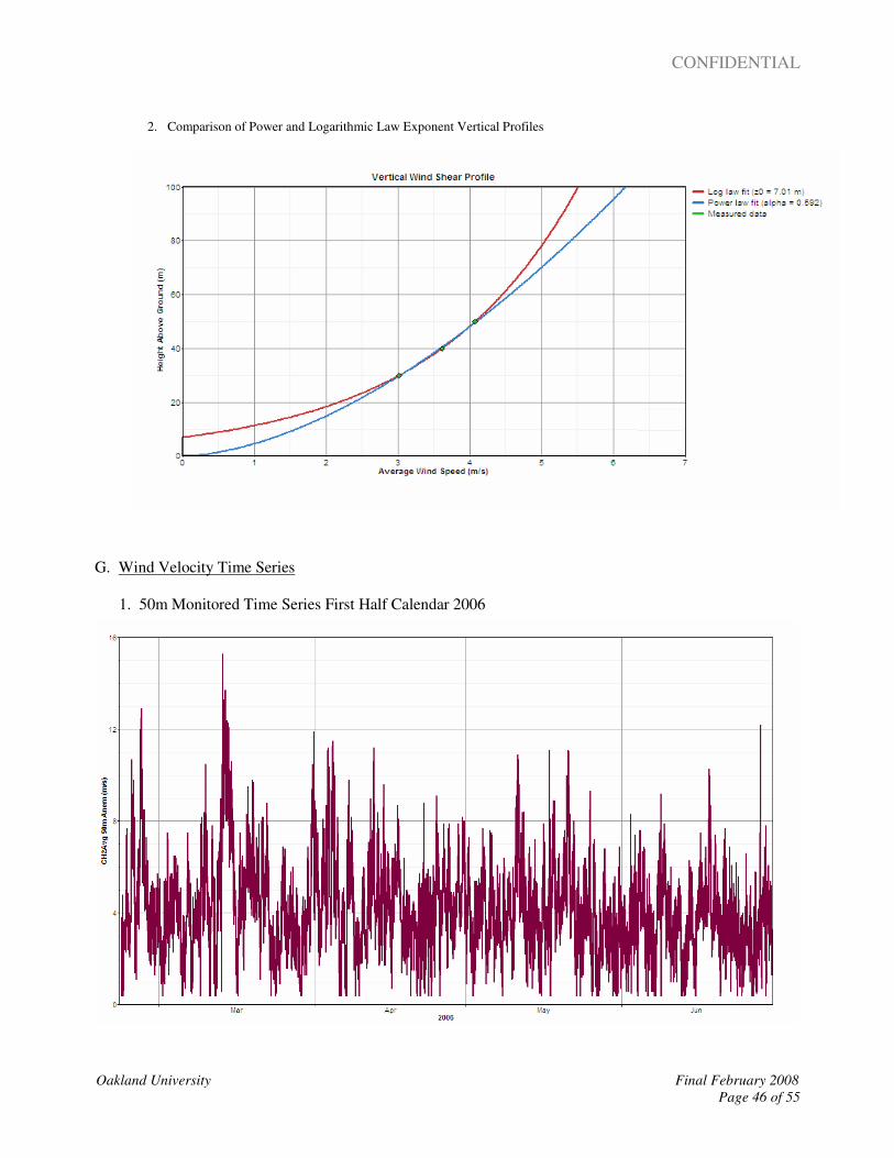
The variation in the wind speed with height above ground can be called the wind shear profile. In the field of
wind resource assessment, analysts typically use one of two mathematical relations to characterize the
measured wind shear profile: a) the logarithmic profile or “Log Law” (red) and b) the power law profile or
“Power Law” (blue) against measured values as seen in the graph on the previous page.
The Log and Power Laws are traditionally used to determine wind velocity estimates at elevations above
metered points, provided data sets for at least two metered points are referenced.
Measurement
Meteorological sensors are intended and designed to monitor specific environmental parameters which
include wind speed, wind direction, temperature and pressure. The measurement of the aforementioned
parameters are required for a number of disciplines, e.g., meteorology and weather forecasting, agriculture,
industrial processing, the study of climate change and for wind turbine generating systems. The requirements
CONFIDENTIAL
Oakland University Final February 2008
Page 17 of 55
for instrument accuracy and reliability are an important consideration when measuring wind velocity for a
profit prognosis in wind generation applications.
The devices that are typically used in the evaluation of a wind regime include:
Device Characteristic Unit of Measure
Anemometer Wind Velocity mph, m/s
Wind Vane Wind Direction degrees
Thermometer Temperature Celsius, Fahrenheit
Barometer Atmospheric Pressure inHg, mbar, kPa
Anemometers
Velocity sensors should be calibrated and certified by a professional testing laboratory. It is the opinion of
management that anemometer should be submitted for calibration after the wind measurement period. This is
because a working anemometer is not likely to be adversely affected by operation in the environment, in such
a manner that would cause the device to record higher wind velocities; rather, the device is more likely
affected by operational wear-and-tear on the pivot points for the bearings, in a manner that would retard wind
velocity measurement.
Hence, having the sensor calibrated after the measuring period, with a minimum of two calibration points
chosen to correspond to the Probability Distribution Function (gathered from the recorded data), would
provide more meaningful quality assurance to the overall accuracy of the wind data and the calculations.
Cup anemometers, like those used in the NGR System installed at Oakland, are the standard method used to
measure wind velocity. This instrument consists of a three-cup assembly (some manufacturers use four cups)
connected to a vertical shaft. The primary advantage of this type of sensor is the degree of linearity of
electronic pulse signal to wind velocity over a given range. The anemometer used has lower sensitivity to
wind turbulence, the skewing of wind caused by the tower and booms. Anemometers do not consume power
from the system while in operation; instead they use a magnetic which is mounted to the shaft of the rotating
cups. Internal to the device is a small induction coil that the poles of the magnet will pass by as it turns. Each
time the magnet passes the coil it generates an electrical pulse that is counted by the data recording logger.

CONFIDENTIAL
Oakland University Final February 2008
Page 18 of 55
This is what is referred to as a magnetic transducer. The pulses are sent down the cable to the data logger
which counts the pulses and applies an engineered conversion multiplier and offset to determine the
tangible wind velocity in units of miles-per-hour (mph) or meters-per-second (m/s).
The traditional conversion factors for mph are: 0.44704 m/s = 1 mph
1 mph =1.1507 knots
Another type of anemometer is the propeller anemometer, which is mounted on a horizontal rotating shaft
oriented into the wind by a tail vane. The propeller anemometer also generates an electric signal that is
proportional to wind velocity. The two sensors have slight differences in responsiveness to fluctuations in
wind speed. According to the wind measurement authorities, there is no clear advantage between the two
devices. The most common anemometer used in the meteorological industry is the cup anemometer for wind
regimes assessments.
The use of redundant anemometers and meteorological towers is highly recommended. The logic is to
minimize the risk of wind speed data being lost because of an anemometer failure. This would effectively be
a loss of primary data that would be used in the calculation of wind power density and wind shear exponents.
Redundant wind sensors, especially at the higher measuring point, are situated so as not to interfere with the
primary sensor. The redundant sensor may also be used to provide substantiation data when the primary
sensor is in the wake of the tower.
Wind Vanes
Wind vanes are used for determining the direction of the wind. The wind vane operates to constantly seek a
position of force equilibrium on both sides of the tailfin by orienting itself into the wind. These devices
typically employ what is referred to as a continuous rotation potentiometer transducer to record direction that
would be relative to the vane itself, accurately to 1º resolution. These instruments consume very low amounts
of power. Care must be taken to align the instrument north marker properly on the tower. Typically, the
mark is set to point toward the center of the tower. After the tower is erected, the orientation of the
instrument boom is then recorded with respect to magnetic north using a compass.
The resolution of the wind vane is important because it is used in determining the direction of wind energy
and thus affects the engineering layout of the wind turbine array (positioning of more than one wind turbine).
CONFIDENTIAL
Oakland University Final February 2008
Page 19 of 55
Adjustments for magnetic declination for compass readings from “true north” and the orientation of the
instrument’s north marker are entered into the software as an offset value.
Atmospheric Pressure Sensors
Air pressure or barometric pressure may be measured in units of kilo-Pascals (kPa), milliBars (mB), or
inches of mercury (inHg). The effect of atmospheric pressure does influence the amount of energy contained
in the wind; contrary to popular opinion, the influence of barometric pressure is relatively low when
compared to wind velocity. Pressure is one of the variables that has a small influence on air density and is not
usually recorded on most test sites. Air density is used to determine wind power density.
Measurement of barometric pressure, when not recorded at the test site, is easily substituted from weather
stations in the region. Barometric pressure is also accurately estimated as a function of site elevation and
temperature.
The traditional conversion constants for barometric pressure are: 1 mB = 100Pa
1kPa = 10 mB
33.8639 mB = 1 inHg
Air Temperature Sensors
There are many different types of temperature sensing technologies that may be employed to measure
temperature. The most common method in field measurement utilizes an integrated circuit (IC). These
integrated circuit sensors use electronics to generate both an internal reference and measured output value.
The effect of atmospheric temperature does influence the amount of energy contained in the wind; contrary
to popular opinion, the influence of temperature is relatively low when compared to wind velocity.
Temperature is one of the variables having a small influence on air density. Air density is used to determine
wind power density. Measurement of temperature, when not recorded at the test site, is easily replicated from
weather stations in the region.
The traditional conversion equations for temperature are: Celsius (C) = (F – 32)/1.8
Kelvin (K) = 273 + C
Fahrenheit (F) = (C x 1.8) + 32
CONFIDENTIAL
Oakland University Final February 2008
Page 20 of 55
Section 4
Factors Affecting Wind Power and Turbine Performance _________________________________________________________________________________________________________________________________________________________________________________________________________________________________________________
A wind turbine generator (WTG) captures the energy of the wind using a rotor having two or more blades,
that is mechanically linked to a generator. As the rotor is forced to turn by prevailing winds, mechanical
energy is removed from the wind and transferred into rotary mechanical force (torque) in the shaft of the
rotor unit. The power that is captured and the speed of rotation, for a rotor system, is dependent on a number
of factors. Some of the main ones are:
� wind velocity
� swept area, number of rotor blades and solidity
� blade pitch
� generator (asynchronous and synchronous)
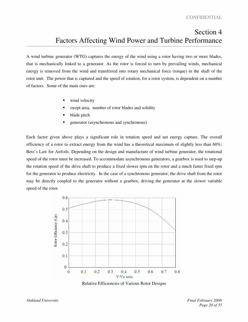
Each factor given above plays a significant role in rotation speed and net energy capture. The overall
efficiency of a rotor to extract energy from the wind has a theoretical maximum of slightly less than 60%;
Betz’s Law for Airfoils. Depending on the design and manufacture of wind turbine generator, the rotational
speed of the rotor must be increased. To accommodate asynchronous generators, a gearbox is used to step-up
the rotation speed of the drive shaft to produce a fixed slower rpm on the rotor and a much faster fixed rpm
for the generator to produce electricity. In the case of a synchronous generator, the drive shaft from the rotor
may be directly coupled to the generator without a gearbox, driving the generator at the slower variable
speed of the rotor.
Relative Efficiencies of Various Rotor Designs
CONFIDENTIAL
Oakland University Final February 2008
Page 21 of 55
Rotor efficiency is not a straightforward topic for the untrained; as an example, when comparing a two-blade
rotor system to that of a three-blade unit, the overall efficiency realized by adding the third blade is on
average increased by only approximately 5%; however, the cost and weight of the three-blade rotor system
block is increased disproportionately by 50%, factoring out the rotor hub and internal sub-assemblies.
A discussion on swept area and solidity is appropriate at this point in our discussion. Swept area is the
circular area that the tips of the rotor blades form as they spin. The swept area is generally given by the
manufacturer in square meters (m2).
A wind turbine generator using a three-blade rotor, where each blade is 27m (≈88.6ft.) in length, will form a
circle 54m (≈177ft.) across the center. This is the rotor diameter. Many manufacturers specify rotor diameter
in the model number of their produce. Swept area for the example above is calculated using the following
basic equation for circular area,
Rotor swept area is important for determining the amount of energy held by the wind passing over the rotor
at a given velocity.
Using the value for swept area, the total power that would be available for conversion by the rotor may not
be determined. Assuming that the power in the prevailing wind, referred to as wind power density (WPD), at
a given moment in time, is determined to be 250 watts (w)/m2; the total power that could be extracted by a
rotor having 100% efficiency becomes,
Power (wind swept area) = WPD x Rotor Swept Area
Power (wind swept area) = 250 w/m2 x 2,290 m2 = 572,500 w (572.5 kW)
Few manufacturers offer the option to change the size of a wind turbine generator’s rotor. When this option
is available, it should be considered carefully, because a larger diameter rotor has more wind flowing across
the blades and converts more kinetic mechanical energy into electrical energy. The added cost for a larger
diameter rotor should be weighed along with the use of higher towers to determine the added economic
benefit for a wind turbine project.
CONFIDENTIAL
Oakland University Final February 2008
Page 22 of 55
To determine the general solidity of the rotor, we must know the amount of active surface area that a rotor
blade will have against the prevailing wind. Let us say that the example rotor blades have a surface area of
40m2. Since this is a three blade rotor, the total active surface area would be 120m
2.
Solidity is the percentage of total blade surface to swept area, 120m2 with respect to 2,290 m
2. We have,
.
The correlation between the speed of rotor rotation and the number of rotor blades (solidity) is an inverse
relationship. That is, as solidity or the number of blades or area is increased, the speed of rotation for a rotor
unit operating in a given wind velocity will decrease.
The number and design of the rotor blades is at the center of the total wind turbine efficiency. Simply stated,
the rotor blades are perhaps the most important factor in capturing wind energy. Rotor blades have the
distinction of being the least efficient subassembly of the wind turbine generator and account for the greatest
energy conversion losses in the entire wind turbine generator.
The efficiency factor of a rotor (Cp), operating in a wind turbine generator, is not constant. A rotor,
independent of the number of blades, will have a maximum or best operating efficiency when the speed of
the rotor movement at its outermost tip (tip speed) is a certain multiple of the prevailing upstream wind
velocity acting on the rotor. The relationship between tip speed and wind speed is referred to, in the industry,
as tip speed ratio (TSR).
A wind turbine generator having a rotor tip speed of 50 m/s (112 mph) and a prevailing wind velocity of 10
m/s (22 mph) would have a TSR of 5.
TSR for a model three-blade rotor may vary between 3 and 7 with rotor efficiencies ranging from 0.25 (25%)
at the lower and upper limits of TSR to 0.45 (45%) at mid-range. Total annual energy capture is severely
affected when the rotor is caused to operate at less than its optimum TSR.
CONFIDENTIAL
Oakland University Final February 2008
Page 23 of 55
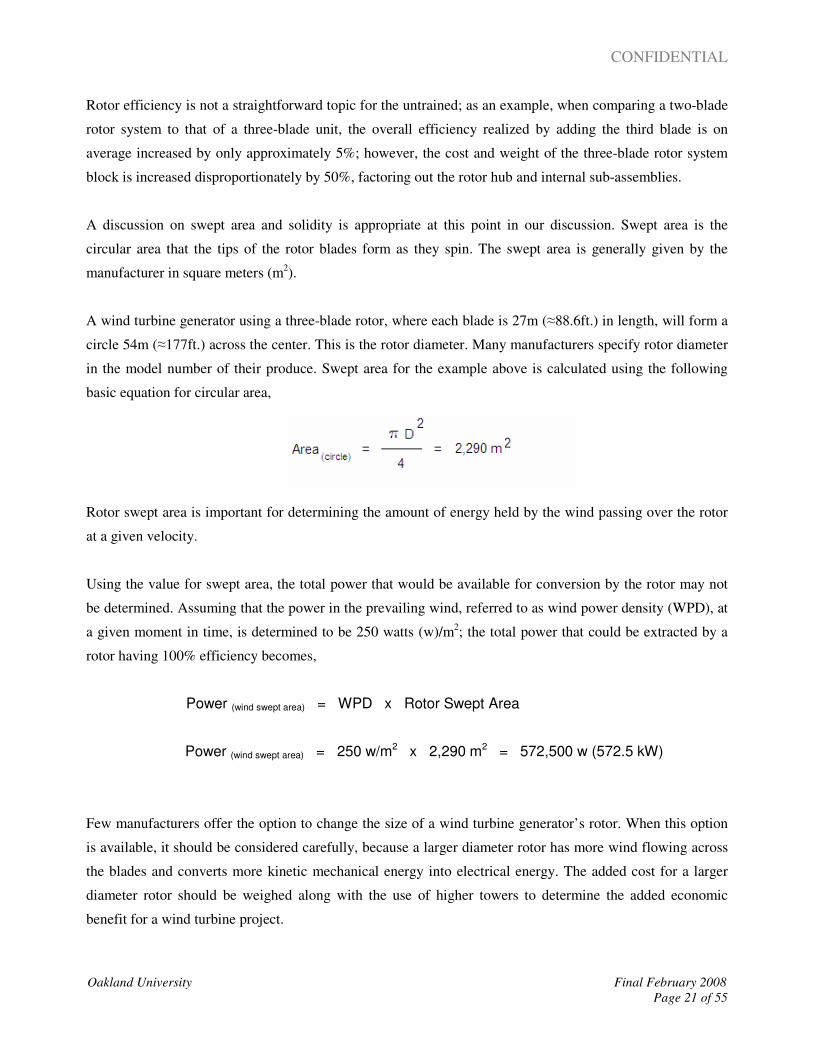
Maintaining an optimum value for TSR is more challenging for the manufacturers of fixed speed wind
turbine generators and less problematic for manufacturers of variable speed machines. Energy capture (kw-h)
is a function of rotor efficiency as seen in the diagram presented below.
Rotor efficiency and annual energy capture versus TSR
As the wind crosses the rotor blades, and power is extracted from it, the velocity of the wind behind the rotor
is reduced in accordance with the efficiency of the rotor design. This will cause a wake or turbulence zone to
develop and trail behind the rotor for several multiples of rotor diameter.
As the wind crosses the rotor blades and power extracted from it, the velocity of the wind behind the rotor is
reduced in accordance with the efficiency of the rotor design. This will cause a wake or turbulence zone
trailing the rotor, where the power in the wind will be reduced for an appreciable distance.

CONFIDENTIAL
Oakland University Final February 2008
Page 24 of 55
Computational fluid dynamics (CFD) is the accepted method for managing turbine wake problems and
elements of micro-siting.
Turbine wake zone shown generating an adverse affect on a second turbine downstream. Modeling with computational fluid dynamic (CFD) software. Courtesy of Fluent, Inc.
The amount of mechanical power that is captured by the rotor from the wind is a function of the difference
between upstream wind velocity (flowing toward the rotor) and downstream wind velocity (passing behind
the rotor). The spacing between wind turbines becomes very important, so that each subsequent downstream
wind turbine has wind flow not significantly reduced in velocity and corresponding power. The historical
wind direction pattern (shown by what is referred to as a wind rose) and the arrangement of multiple turbines
(turbine array alignment) must seek to optimize wind flow to each turbine for energy generation.
Every practical wind turbine array design will lose some of the potential energy in the wind because of
reduced wind flow from one or more combined turbines. The term used to describe power loss due to the
placement patterns of turbines is “array loss”. The solution for minimizing array loss is to lay out the turbine
pattern and unit separation with special software and engineering considerate to real estate availability,
proposed installation pattern, construction costs and variations in wind direction.
CONFIDENTIAL
Oakland University Final February 2008
Page 25 of 55
D0
D5 D7
D9 D11
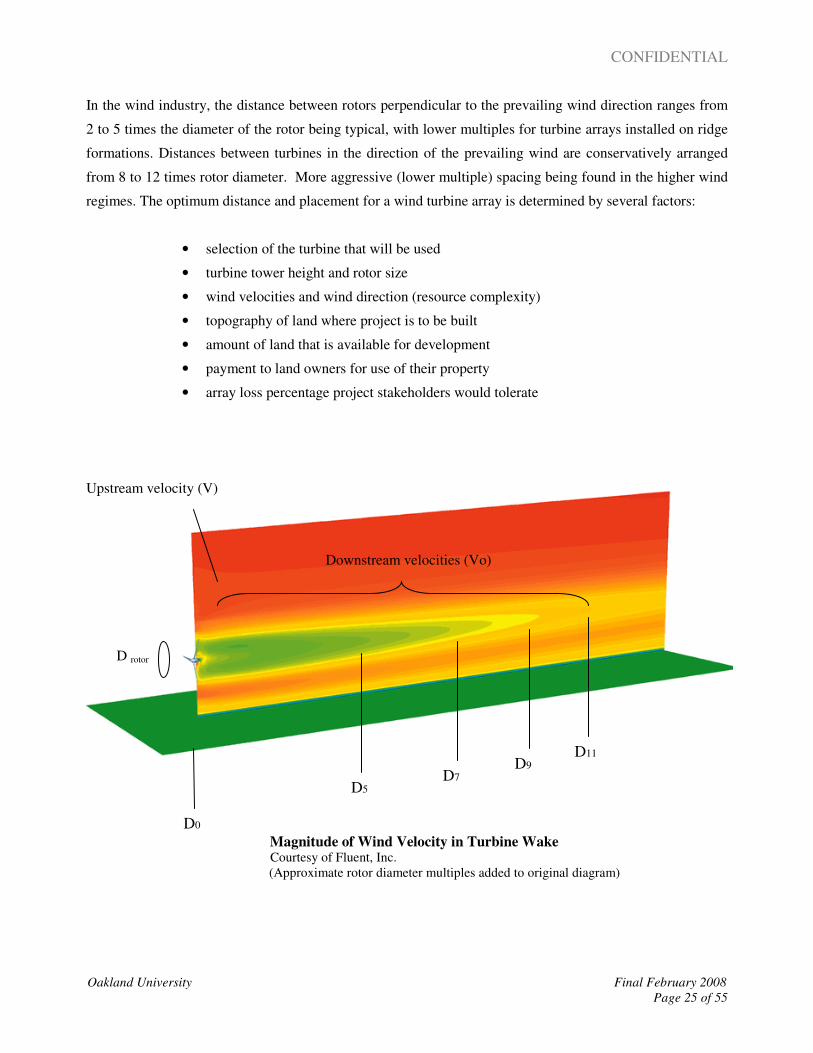
In the wind industry, the distance between rotors perpendicular to the prevailing wind direction ranges from
2 to 5 times the diameter of the rotor being typical, with lower multiples for turbine arrays installed on ridge
formations. Distances between turbines in the direction of the prevailing wind are conservatively arranged
from 8 to 12 times rotor diameter. More aggressive (lower multiple) spacing being found in the higher wind
regimes. The optimum distance and placement for a wind turbine array is determined by several factors:
• selection of the turbine that will be used
• turbine tower height and rotor size
• wind velocities and wind direction (resource complexity)
• topography of land where project is to be built
• amount of land that is available for development
• payment to land owners for use of their property
• array loss percentage project stakeholders would tolerate
Upstream velocity (V)
Downstream velocities (Vo)
D rotor
Magnitude of Wind Velocity in Turbine Wake Courtesy of Fluent, Inc.
(Approximate rotor diameter multiples added to original diagram)

CONFIDENTIAL
Oakland University Final February 2008
Page 26 of 55
Relatively speaking, the placement of a wind turbine at position D5 within the array plan would produce less
energy capture than an identical turbine placed at position D11. In the latter position, wind turbulence is lower
and has become a more laminar fluid flow. High wake turbulence will also increase rotor fatigue and failure
rates adding increased operational and maintenance costs for the facility.
The energy that is contained in the wind may be found using the following equation:
where P is the mechanical power (kWmech),
ρ is the density of air (1.225 kg/m3),
A is the area swept by the rotor, and
V is the wind velocity (m/s).
Using the above equation, a wind blowing with an average velocity of 7.0 m/s over a rotor of 1m2 will have a
wind power density of 210w/m2. If we use the rotor having 2,290 m
2 or swept area, the mechanical power in
the wind available to the rotor would be 481,100 w (481.1 kW).
The value of mechanical power extracted from the wind when the upstream and downstream wind velocities
are known is calculated utilizing the equation:
[ ]
where Po is the mechanical power extracted (kWmech),
V is the upstream wind velocity (m/s), and
Vo is the downstream wind velocity (m/s)
For example, if the upstream wind velocity is 7.0 m/s and the downstream wind velocity behind the rotor is
measured at 5.0 m/s, the rotor would have captured 201,978 w (201.9kW). The ratio of downstream wind
velocity (Vo) to upstream wind velocity (V) for this example would be 0.714. Inspecting the graph, we find
that the V/Vo ratio of 0.714 intersects with a rotor efficiency of 0.42.
CONFIDENTIAL
Oakland University Final February 2008
Page 27 of 55
Wind Velocity
(m/s)
Wind Power Density
(w/m2)
1 1
2 5
3 17
4 39
5 77
6 132
7 210
8 314
9 447
10 613
11 815
12 1,058
13 1,346
14 1,681
15 2,067
16 2,509
17 3,009
18 3,572
19 4,201
20 4,900
21 5,672
22 6,522
23 7,452
Wind Power Density Table
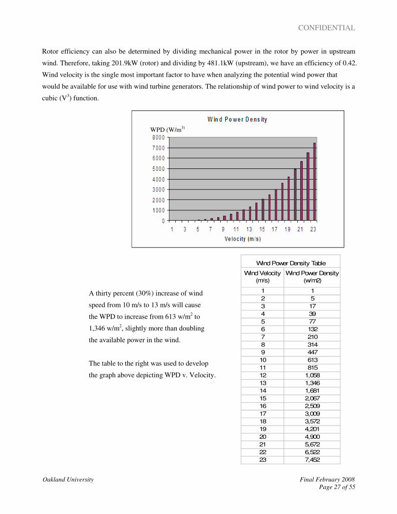
Rotor efficiency can also be determined by dividing mechanical power in the rotor by power in upstream
wind. Therefore, taking 201.9kW (rotor) and dividing by 481.1kW (upstream), we have an efficiency of 0.42.
Wind velocity is the single most important factor to have when analyzing the potential wind power that
would be available for use with wind turbine generators. The relationship of wind power to wind velocity is a
cubic (V3) function.
WPD (W/m3)
A thirty percent (30%) increase of wind
speed from 10 m/s to 13 m/s will cause
the WPD to increase from 613 w/m2 to
1,346 w/m2, slightly more than doubling
the available power in the wind.
The table to the right was used to develop
the graph above depicting WPD v. Velocity.

CONFIDENTIAL
Oakland University Final February 2008
Page 28 of 55
n = 1ΣWPD =
n1
2n
3 Vρ
Air density (ρ) is, nevertheless, another factor which will influence the amount of energy that a wind turbine
generator will glean from the wind. The relationship between air density and energy capture is directly
proportional, meaning that air flow that has ten percent greater air density will have ten percent more wind
power available for conversion into electricity by the wind turbine.
Air density is affected by two variables, explicitly, ambient temperature and the barometric (atmospheric)
pressure. The traditional equation for finding air density is,
Where R is the physical specific gas constant (287 J kg -1
K -1
),
Р is the air pressure in Pascal (Pa) or Newton/m2 (N/m
2), and
T is the temperature in °K.
From the equation given above, we see that at as the ambient temperature of air increases, the air density will
decrease; while increased barometric pressure will result in higher air density as well. Therefore, wind flow
caused by nearby low pressure systems will tend to have greater power available in the wind. It is also
reasonable to state cooler climactic and seasonal winds will have increased power relative to other conditions
for the region being studied.
This is one of the equations that is used to calculate the power in the wind at a given velocity. It is also the
root formula for determining wind power density (WPD) for a test site.
The equations make use of the density of air ( ρ ). Density of air is dependent upon temperature and
barometric pressure.
Wind Velocity Distribution
Probability Distribution Function is important to know the distribution of the wind velocity in terms of the
number of hours of wind at a particular velocity. This gives a better calculation of wind power at a given site
that is being evaluated. Knowing the average wind speed is helpful, but not as valuable as velocity
distribution.
ρ =
P
R T

CONFIDENTIAL
Oakland University Final February 2008
Page 29 of 55
A given wind site may have an average wind speed of 7 m/s. Depending on the distribution of wind, the site
may have a good resource or a weaker resource as exemplified in the following example.
Case 1: Average wind speed 7.0 m/s during a three-hour time period.
Hour #1: 5 m/s
Hour #2: 10 m/s
Hour #3: 6 m/s
P1 = 0.5 x 1.225 x 53 = 76 w/m
2
P2 = 0.5 x 1.225 x 103 = 612 w/m
2
P3 = 0.5 x 1.225 x 63 = 132 w/m
2
Average: 273 w/m2
Case 2: Average wind speed 7.0 m/s during a three-hour time period.
Hour #1: 5 m/s
Hour #2: 5 m/s
Hour #3: 11 m.s
P1 = 0.5 x 1.225 x 53 = 76 w/m
2
P2 = 0.5 x 1.225 x 53 = 76 w/m
2
P3 = 0.5 x 1.225 x 113 = 815 w/m
2
Average: 322 w/m2
Each three-hour period given above again has the same average wind speed; the average wind of 7 m/s with
the distribution shown in Case 2 would have provided more available wind energy for conversion into
electrical energy and would be considered a better wind power resource.
CONFIDENTIAL
Oakland University Final February 2008
Page 30 of 55
Section 5
Data Validation and Reporting _________________________________________________________________________________________________________________________________________________________________________________________________________________________________________________
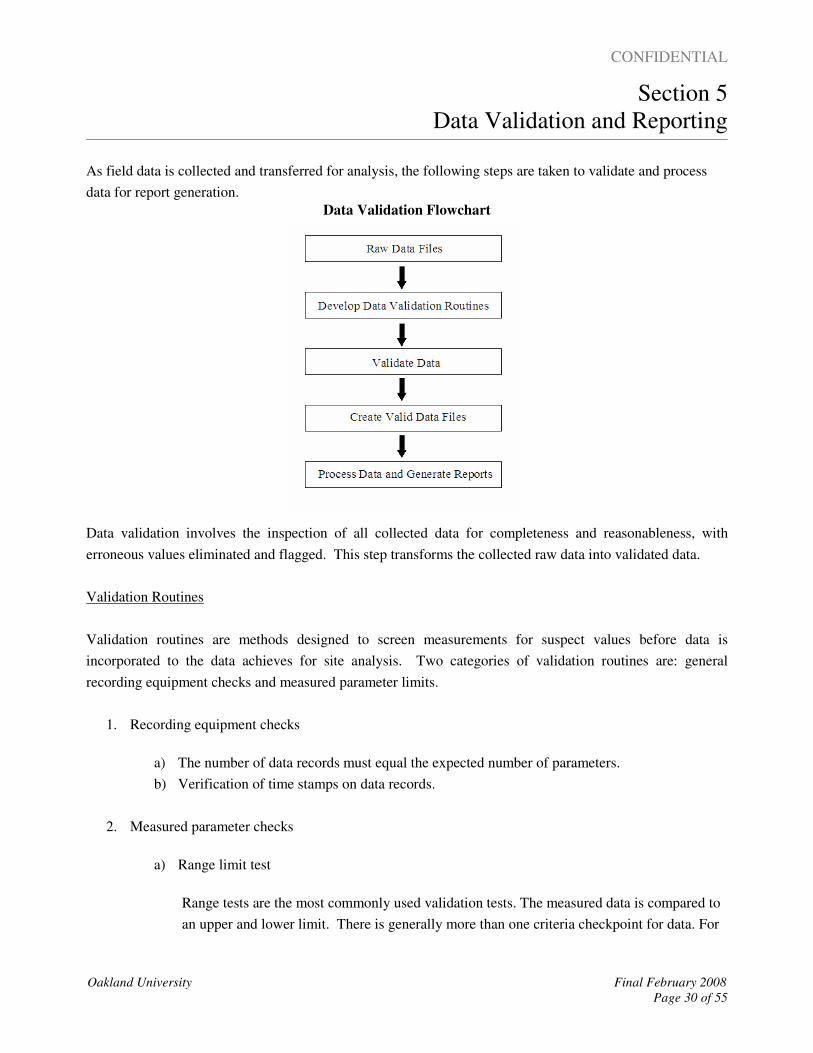
As field data is collected and transferred for analysis, the following steps are taken to validate and process
data for report generation.
Data Validation Flowchart
Data validation involves the inspection of all collected data for completeness and reasonableness, with
erroneous values eliminated and flagged. This step transforms the collected raw data into validated data.
Validation Routines
Validation routines are methods designed to screen measurements for suspect values before data is
incorporated to the data achieves for site analysis. Two categories of validation routines are: general
recording equipment checks and measured parameter limits.
1. Recording equipment checks
a) The number of data records must equal the expected number of parameters.
b) Verification of time stamps on data records.
2. Measured parameter checks
a) Range limit test
Range tests are the most commonly used validation tests. The measured data is compared to
an upper and lower limit. There is generally more than one criteria checkpoint for data. For

CONFIDENTIAL
Oakland University Final February 2008
Page 31 of 55
example, you may set a range parameter for an anemometer between 0 m/s and
20 m/s; this is fine for the summer months, but during the winter icing may occur
and strong winds may be present. A frozen anemometer will not be flagged if
speed is the only criteria.
b) Physical relational test
This is a comparison based test on metered data. The comparison is predicated on
anticipated physical relationships between parameters. When the unanticipated
relationship occurs between measured parameters, it is flagged and investigated
before being accepted as valid data. An obvious example would be a higher wind
velocity being recorded on the 30m anemometer when compared to the 50m
anemometer.
c) Examination of trend
This type of test is based on “rate of change” in the measured parameter’s value.
An example of a trend test that would be flagged for inspection would be a change of
temperature from 20 ºC to 10 ºC in 10 minutes time.
Treatment of Missing Data
Data that has been put to the various validation checks will either be passed as valid or flagged as suspect
data. The handling of suspect data is as follows:
� Notation on file and record for individual performing analysis
� Substitute alternate sensor metric for suspect data cell if deemed invalid

CONFIDENTIAL
Oakland University Final February 2008
Page 32 of 55
Section 6
Collected Wind Data _________________________________________________________________________________________________________________________________________________________________________________________________________________________________________________
The data in the following section represents select collected data for the purpose of this wind study.
Data is provided in either table or graphic pictorial for the benefit of the reader.
The following data is given as recorded and without modification:
I. Tabular Format
A. Monthly and Annual Stats
1. 50m Wind Velocity (m/s)
2. 40m Wind Velocity (m/s)
3. 30m Wind Velocity (m/s)
4. Temperature (Celsius)
5. Surface Roughness (m)
6. Log Law Exponents
7. 50m Wind Directivity
B. Probability Distribution Bins
1. 50m Wind Velocity (m/s)
2. 40m Wind Velocity (m/s)
3. 30m Wind Velocity (m/s)
II. Graphic Format
A. Distribution Curves
1. 50m Wind Velocity (m/s)
2. 40m Wind Velocity (m/s)
3. 30m Wind Velocity (m/s)
B. Seasonal Wind Profile
C. Diurnal Curve Family for 30m, 40m and 50m Wind Velocity
D. Wind Roses
1. 50m Mean Value by Direction
2. 50m Total Value by Direction
E. Wind Turbulence
F. Wind Shear
G. Wind Velocity Time Series
1. 50m Monitored Time Series First Half Calendar 2006
2. 50m Monitored Time Series Second Half Calendar 2006
3. 50m Monitored Time Series First Half Calendar 2007
4. 50m Monitored Time Series Second Half Calendar 2007
CONFIDENTIAL
Oakland University Final February 2008
Page 33 of 55
I. Tabular Format
A. Monthly and Annual Stats
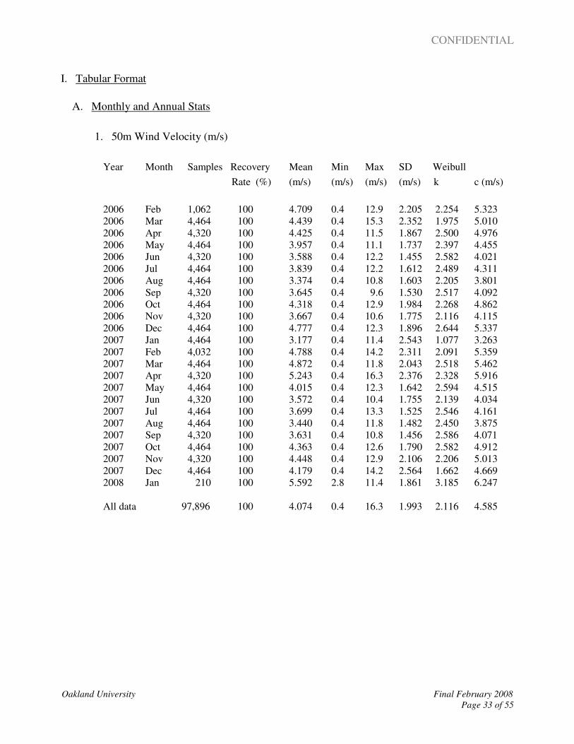
1. 50m Wind Velocity (m/s)
Year Month Samples Recovery Mean Min Max SD Weibull
Rate (%) (m/s) (m/s) (m/s) (m/s) k c (m/s)
2006 Feb 1,062 100 4.709 0.4 12.9 2.205 2.254 5.323
2006 Mar 4,464 100 4.439 0.4 15.3 2.352 1.975 5.010
2006 Apr 4,320 100 4.425 0.4 11.5 1.867 2.500 4.976
2006 May 4,464 100 3.957 0.4 11.1 1.737 2.397 4.455
2006 Jun 4,320 100 3.588 0.4 12.2 1.455 2.582 4.021
2006 Jul 4,464 100 3.839 0.4 12.2 1.612 2.489 4.311
2006 Aug 4,464 100 3.374 0.4 10.8 1.603 2.205 3.801
2006 Sep 4,320 100 3.645 0.4 9.6 1.530 2.517 4.092
2006 Oct 4,464 100 4.318 0.4 12.9 1.984 2.268 4.862
2006 Nov 4,320 100 3.667 0.4 10.6 1.775 2.116 4.115
2006 Dec 4,464 100 4.777 0.4 12.3 1.896 2.644 5.337
2007 Jan 4,464 100 3.177 0.4 11.4 2.543 1.077 3.263
2007 Feb 4,032 100 4.788 0.4 14.2 2.311 2.091 5.359
2007 Mar 4,464 100 4.872 0.4 11.8 2.043 2.518 5.462
2007 Apr 4,320 100 5.243 0.4 16.3 2.376 2.328 5.916
2007 May 4,464 100 4.015 0.4 12.3 1.642 2.594 4.515
2007 Jun 4,320 100 3.572 0.4 10.4 1.755 2.139 4.034
2007 Jul 4,464 100 3.699 0.4 13.3 1.525 2.546 4.161
2007 Aug 4,464 100 3.440 0.4 11.8 1.482 2.450 3.875
2007 Sep 4,320 100 3.631 0.4 10.8 1.456 2.586 4.071
2007 Oct 4,464 100 4.363 0.4 12.6 1.790 2.582 4.912
2007 Nov 4,320 100 4.448 0.4 12.9 2.106 2.206 5.013
2007 Dec 4,464 100 4.179 0.4 14.2 2.564 1.662 4.669
2008 Jan 210 100 5.592 2.8 11.4 1.861 3.185 6.247
All data 97,896 100 4.074 0.4 16.3 1.993 2.116 4.585
CONFIDENTIAL
Oakland University Final February 2008
Page 34 of 55
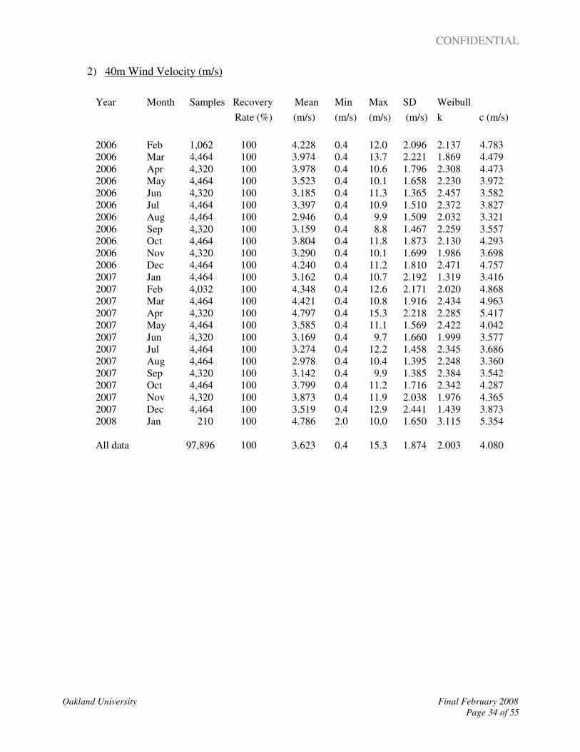
2) 40m Wind Velocity (m/s)
Year Month Samples Recovery Mean Min Max SD Weibull
Rate (%) (m/s) (m/s) (m/s) (m/s) k c (m/s)
2006 Feb 1,062 100 4.228 0.4 12.0 2.096 2.137 4.783
2006 Mar 4,464 100 3.974 0.4 13.7 2.221 1.869 4.479
2006 Apr 4,320 100 3.978 0.4 10.6 1.796 2.308 4.473
2006 May 4,464 100 3.523 0.4 10.1 1.658 2.230 3.972
2006 Jun 4,320 100 3.185 0.4 11.3 1.365 2.457 3.582
2006 Jul 4,464 100 3.397 0.4 10.9 1.510 2.372 3.827
2006 Aug 4,464 100 2.946 0.4 9.9 1.509 2.032 3.321
2006 Sep 4,320 100 3.159 0.4 8.8 1.467 2.259 3.557
2006 Oct 4,464 100 3.804 0.4 11.8 1.873 2.130 4.293
2006 Nov 4,320 100 3.290 0.4 10.1 1.699 1.986 3.698
2006 Dec 4,464 100 4.240 0.4 11.2 1.810 2.471 4.757
2007 Jan 4,464 100 3.162 0.4 10.7 2.192 1.319 3.416
2007 Feb 4,032 100 4.348 0.4 12.6 2.171 2.020 4.868
2007 Mar 4,464 100 4.421 0.4 10.8 1.916 2.434 4.963
2007 Apr 4,320 100 4.797 0.4 15.3 2.218 2.285 5.417
2007 May 4,464 100 3.585 0.4 11.1 1.569 2.422 4.042
2007 Jun 4,320 100 3.169 0.4 9.7 1.660 1.999 3.577
2007 Jul 4,464 100 3.274 0.4 12.2 1.458 2.345 3.686
2007 Aug 4,464 100 2.978 0.4 10.4 1.395 2.248 3.360
2007 Sep 4,320 100 3.142 0.4 9.9 1.385 2.384 3.542
2007 Oct 4,464 100 3.799 0.4 11.2 1.716 2.342 4.287
2007 Nov 4,320 100 3.873 0.4 11.9 2.038 1.976 4.365
2007 Dec 4,464 100 3.519 0.4 12.9 2.441 1.439 3.873
2008 Jan 210 100 4.786 2.0 10.0 1.650 3.115 5.354
All data 97,896 100 3.623 0.4 15.3 1.874 2.003 4.080
CONFIDENTIAL
Oakland University Final February 2008
Page 35 of 55
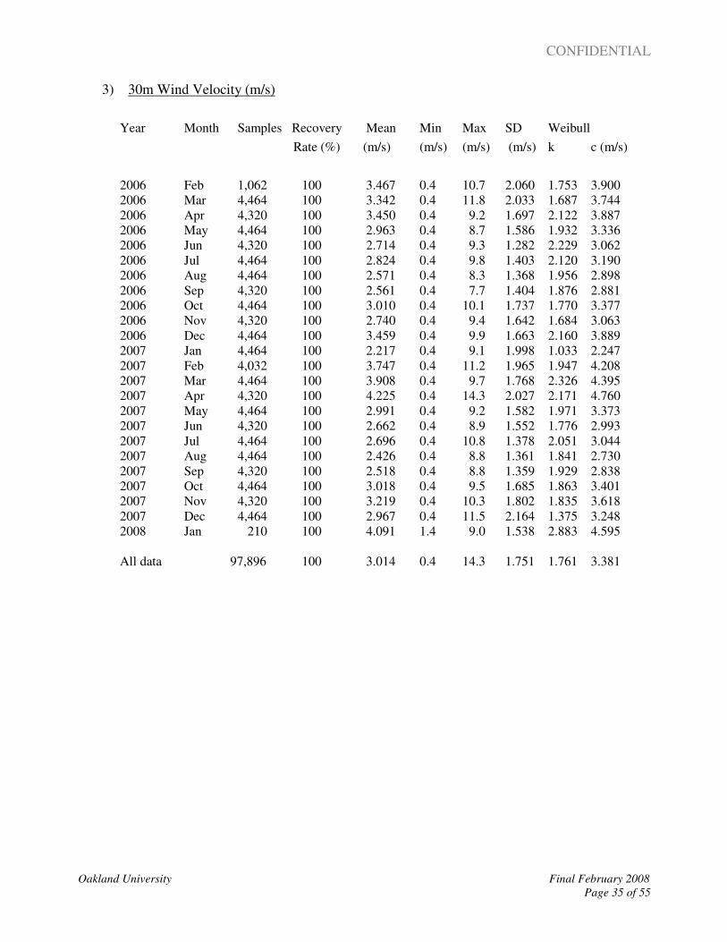
3) 30m Wind Velocity (m/s)
Year Month Samples Recovery Mean Min Max SD Weibull
Rate (%) (m/s) (m/s) (m/s) (m/s) k c (m/s)
2006 Feb 1,062 100 3.467 0.4 10.7 2.060 1.753 3.900
2006 Mar 4,464 100 3.342 0.4 11.8 2.033 1.687 3.744
2006 Apr 4,320 100 3.450 0.4 9.2 1.697 2.122 3.887
2006 May 4,464 100 2.963 0.4 8.7 1.586 1.932 3.336
2006 Jun 4,320 100 2.714 0.4 9.3 1.282 2.229 3.062
2006 Jul 4,464 100 2.824 0.4 9.8 1.403 2.120 3.190
2006 Aug 4,464 100 2.571 0.4 8.3 1.368 1.956 2.898
2006 Sep 4,320 100 2.561 0.4 7.7 1.404 1.876 2.881
2006 Oct 4,464 100 3.010 0.4 10.1 1.737 1.770 3.377
2006 Nov 4,320 100 2.740 0.4 9.4 1.642 1.684 3.063
2006 Dec 4,464 100 3.459 0.4 9.9 1.663 2.160 3.889
2007 Jan 4,464 100 2.217 0.4 9.1 1.998 1.033 2.247
2007 Feb 4,032 100 3.747 0.4 11.2 1.965 1.947 4.208
2007 Mar 4,464 100 3.908 0.4 9.7 1.768 2.326 4.395
2007 Apr 4,320 100 4.225 0.4 14.3 2.027 2.171 4.760
2007 May 4,464 100 2.991 0.4 9.2 1.582 1.971 3.373
2007 Jun 4,320 100 2.662 0.4 8.9 1.552 1.776 2.993
2007 Jul 4,464 100 2.696 0.4 10.8 1.378 2.051 3.044
2007 Aug 4,464 100 2.426 0.4 8.8 1.361 1.841 2.730
2007 Sep 4,320 100 2.518 0.4 8.8 1.359 1.929 2.838
2007 Oct 4,464 100 3.018 0.4 9.5 1.685 1.863 3.401
2007 Nov 4,320 100 3.219 0.4 10.3 1.802 1.835 3.618
2007 Dec 4,464 100 2.967 0.4 11.5 2.164 1.375 3.248
2008 Jan 210 100 4.091 1.4 9.0 1.538 2.883 4.595
All data 97,896 100 3.014 0.4 14.3 1.751 1.761 3.381
CONFIDENTIAL
Oakland University Final February 2008
Page 36 of 55
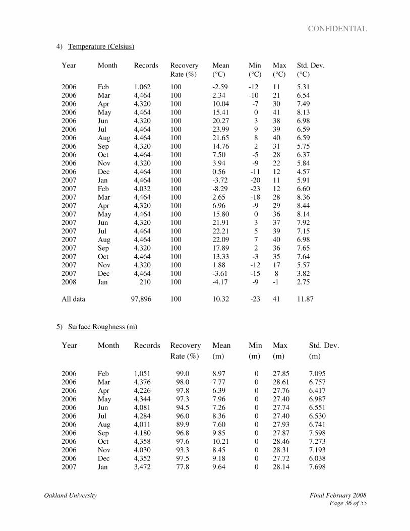
4) Temperature (Celsius)
Year Month Records Recovery Mean Min Max Std. Dev.
Rate (%) (°C) (°C) (°C) (°C)
2006 Feb 1,062 100 -2.59 -12 11 5.31
2006 Mar 4,464 100 2.34 -10 21 6.54
2006 Apr 4,320 100 10.04 -7 30 7.49
2006 May 4,464 100 15.41 0 41 8.13
2006 Jun 4,320 100 20.27 3 38 6.98
2006 Jul 4,464 100 23.99 9 39 6.59
2006 Aug 4,464 100 21.65 8 40 6.59
2006 Sep 4,320 100 14.76 2 31 5.75
2006 Oct 4,464 100 7.50 -5 28 6.37
2006 Nov 4,320 100 3.94 -9 22 5.84
2006 Dec 4,464 100 0.56 -11 12 4.57
2007 Jan 4,464 100 -3.72 -20 11 5.91
2007 Feb 4,032 100 -8.29 -23 12 6.60
2007 Mar 4,464 100 2.65 -18 28 8.36
2007 Apr 4,320 100 6.96 -9 29 8.44
2007 May 4,464 100 15.80 0 36 8.14
2007 Jun 4,320 100 21.91 3 37 7.92
2007 Jul 4,464 100 22.21 5 39 7.15
2007 Aug 4,464 100 22.09 7 40 6.98
2007 Sep 4,320 100 17.89 2 36 7.65
2007 Oct 4,464 100 13.33 -3 35 7.64
2007 Nov 4,320 100 1.88 -12 17 5.57
2007 Dec 4,464 100 -3.61 -15 8 3.82
2008 Jan 210 100 -4.17 -9 -1 2.75
All data 97,896 100 10.32 -23 41 11.87
5) Surface Roughness (m)
Year Month Records Recovery Mean Min Max Std. Dev.
Rate (%) (m) (m) (m) (m)
2006 Feb 1,051 99.0 8.97 0 27.85 7.095
2006 Mar 4,376 98.0 7.77 0 28.61 6.757
2006 Apr 4,226 97.8 6.39 0 27.76 6.417
2006 May 4,344 97.3 7.96 0 27.40 6.987
2006 Jun 4,081 94.5 7.26 0 27.74 6.551
2006 Jul 4,284 96.0 8.36 0 27.40 6.530
2006 Aug 4,011 89.9 7.60 0 27.93 6.741
2006 Sep 4,180 96.8 9.85 0 27.87 7.598
2006 Oct 4,358 97.6 10.21 0 28.46 7.273
2006 Nov 4,030 93.3 8.45 0 28.31 7.193
2006 Dec 4,352 97.5 9.18 0 27.72 6.038
2007 Jan 3,472 77.8 9.64 0 28.14 7.698
CONFIDENTIAL
Oakland University Final February 2008
Page 37 of 55
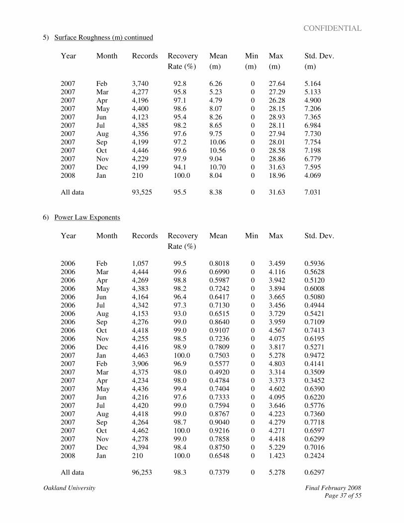
5) Surface Roughness (m) continued
Year Month Records Recovery Mean Min Max Std. Dev.
Rate (%) (m) (m) (m) (m)
2007 Feb 3,740 92.8 6.26 0 27.64 5.164
2007 Mar 4,277 95.8 5.23 0 27.29 5.133
2007 Apr 4,196 97.1 4.79 0 26.28 4.900
2007 May 4,400 98.6 8.07 0 28.15 7.206
2007 Jun 4,123 95.4 8.26 0 28.93 7.365
2007 Jul 4,385 98.2 8.65 0 28.11 6.984
2007 Aug 4,356 97.6 9.75 0 27.94 7.730
2007 Sep 4,199 97.2 10.06 0 28.01 7.754
2007 Oct 4,446 99.6 10.56 0 28.58 7.198
2007 Nov 4,229 97.9 9.04 0 28.86 6.779
2007 Dec 4,199 94.1 10.70 0 31.63 7.595
2008 Jan 210 100.0 8.04 0 18.96 4.069
All data 93,525 95.5 8.38 0 31.63 7.031
6) Power Law Exponents
Year Month Records Recovery Mean Min Max Std. Dev.
Rate (%)
2006 Feb 1,057 99.5 0.8018 0 3.459 0.5936
2006 Mar 4,444 99.6 0.6990 0 4.116 0.5628
2006 Apr 4,269 98.8 0.5987 0 3.942 0.5120
2006 May 4,383 98.2 0.7242 0 3.894 0.6008
2006 Jun 4,164 96.4 0.6417 0 3.665 0.5080
2006 Jul 4,342 97.3 0.7130 0 3.456 0.4944
2006 Aug 4,153 93.0 0.6515 0 3.729 0.5421
2006 Sep 4,276 99.0 0.8640 0 3.959 0.7109
2006 Oct 4,418 99.0 0.9107 0 4.567 0.7413
2006 Nov 4,255 98.5 0.7236 0 4.075 0.6195
2006 Dec 4,416 98.9 0.7809 0 3.817 0.5271
2007 Jan 4,463 100.0 0.7503 0 5.278 0.9472
2007 Feb 3,906 96.9 0.5577 0 4.803 0.4141
2007 Mar 4,375 98.0 0.4920 0 3.314 0.3509
2007 Apr 4,234 98.0 0.4784 0 3.373 0.3452
2007 May 4,436 99.4 0.7404 0 4.602 0.6390
2007 Jun 4,216 97.6 0.7333 0 4.095 0.6220
2007 Jul 4,420 99.0 0.7594 0 3.646 0.5776
2007 Aug 4,418 99.0 0.8767 0 4.223 0.7360
2007 Sep 4,264 98.7 0.9040 0 4.279 0.7718
2007 Oct 4,462 100.0 0.9216 0 4.271 0.6597
2007 Nov 4,278 99.0 0.7858 0 4.418 0.6299
2007 Dec 4,394 98.4 0.8750 0 5.229 0.7016
2008 Jan 210 100.0 0.6548 0 1.423 0.2424
All data 96,253 98.3 0.7379 0 5.278 0.6297
CONFIDENTIAL
Oakland University Final February 2008
Page 38 of 55
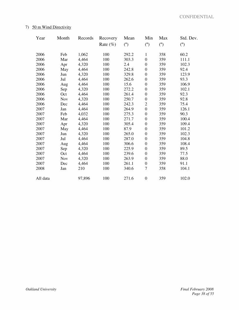
7) 50 m Wind Directivity
Year Month Records Recovery Mean Min Max Std. Dev.
Rate (%) (º) (º) (º) (º)
2006 Feb 1,062 100 292.2 1 358 60.2
2006 Mar 4,464 100 303.3 0 359 111.1
2006 Apr 4,320 100 2.4 0 359 102.3
2006 May 4,464 100 242.8 0 359 92.4
2006 Jun 4,320 100 329.8 0 359 123.9
2006 Jul 4,464 100 262.6 0 359 93.3
2006 Aug 4,464 100 15.6 0 359 106.9
2006 Sep 4,320 100 272.2 0 359 102.1
2006 Oct 4,464 100 261.4 0 359 92.3
2006 Nov 4,320 100 250.7 0 359 92.8
2006 Dec 4,464 100 242.3 2 359 75.4
2007 Jan 4,464 100 264.9 0 359 126.1
2007 Feb 4,032 100 275.3 0 359 90.3
2007 Mar 4,464 100 271.7 0 359 100.4
2007 Apr 4,320 100 305.4 0 359 109.4
2007 May 4,464 100 87.9 0 359 101.2
2007 Jun 4,320 100 265.0 0 359 102.3
2007 Jul 4,464 100 287.0 0 359 104.8
2007 Aug 4,464 100 306.6 0 359 108.4
2007 Sep 4,320 100 225.9 0 359 89.5
2007 Oct 4,464 100 239.6 0 359 77.5
2007 Nov 4,320 100 263.9 0 359 88.0
2007 Dec 4,464 100 261.1 0 359 91.1
2008 Jan 210 100 340.6 7 358 104.1
All data 97,896 100 271.6 0 359 102.0
CONFIDENTIAL
Oakland University Final February 2008
Page 39 of 55
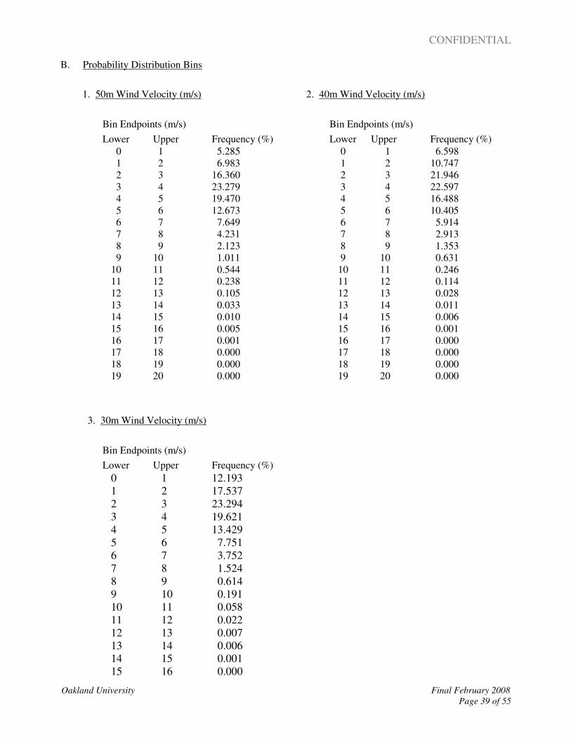
B. Probability Distribution Bins
1. 50m Wind Velocity (m/s) 2. 40m Wind Velocity (m/s)
Bin Endpoints (m/s) Bin Endpoints (m/s)
Lower Upper Frequency (%) Lower Upper Frequency (%)
0 1 5.285 0 1 6.598
1 2 6.983 1 2 10.747
2 3 16.360 2 3 21.946
3 4 23.279 3 4 22.597
4 5 19.470 4 5 16.488
5 6 12.673 5 6 10.405
6 7 7.649 6 7 5.914
7 8 4.231 7 8 2.913
8 9 2.123 8 9 1.353
9 10 1.011 9 10 0.631
10 11 0.544 10 11 0.246
11 12 0.238 11 12 0.114
12 13 0.105 12 13 0.028
13 14 0.033 13 14 0.011
14 15 0.010 14 15 0.006
15 16 0.005 15 16 0.001
16 17 0.001 16 17 0.000
17 18 0.000 17 18 0.000
18 19 0.000 18 19 0.000
19 20 0.000 19 20 0.000
3. 30m Wind Velocity (m/s)
Bin Endpoints (m/s)
Lower Upper Frequency (%)
0 1 12.193
1 2 17.537
2 3 23.294
3 4 19.621
4 5 13.429
5 6 7.751
6 7 3.752
7 8 1.524
8 9 0.614
9 10 0.191
10 11 0.058
11 12 0.022
12 13 0.007
13 14 0.006
14 15 0.001
15 16 0.000
CONFIDENTIAL
Oakland University Final February 2008
Page 40 of 55
3. 30m Wind Velocity (m/s) continued
Bin Endpoints (m/s)
Lower Upper Frequency (%)
16 17 0.001
17 18 0.000
18 19 0.000
19 20 0.000
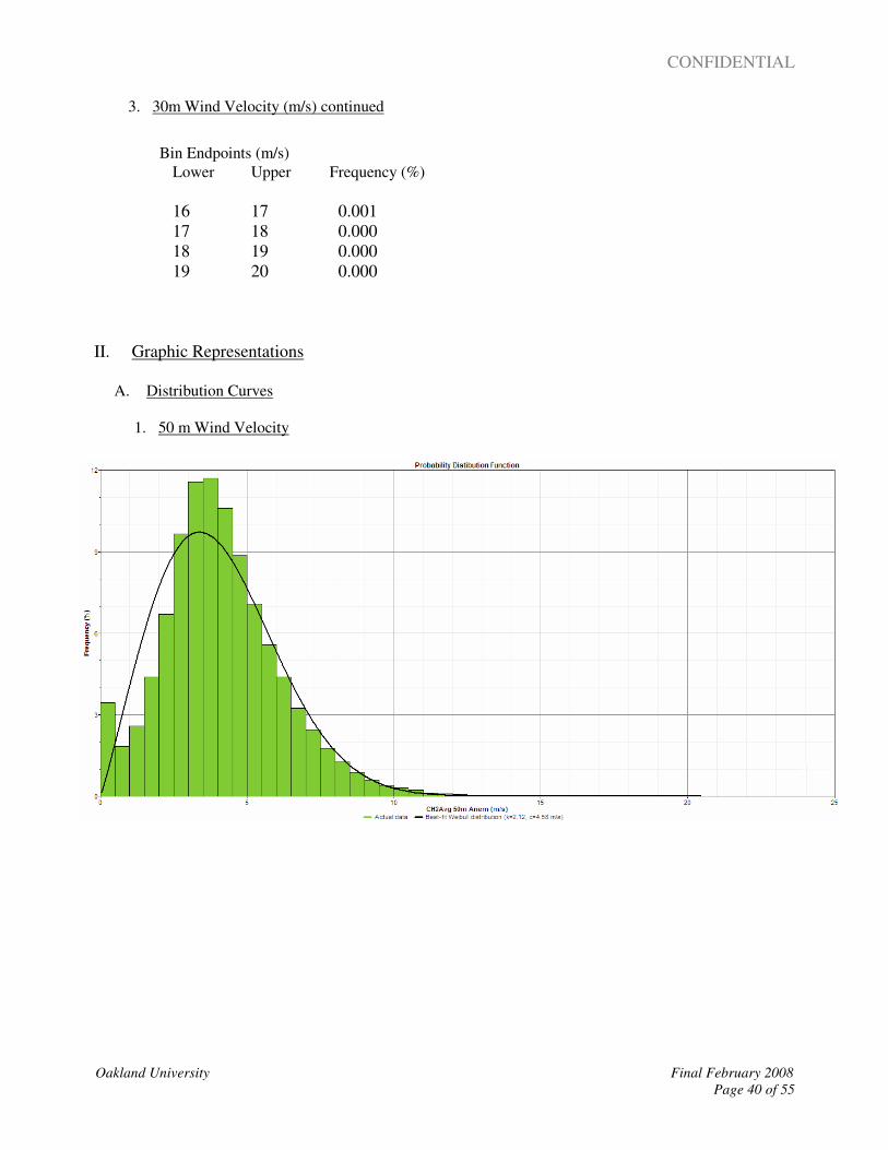
II. Graphic Representations
A. Distribution Curves
1. 50 m Wind Velocity
CONFIDENTIAL
Oakland University Final February 2008
Page 41 of 55
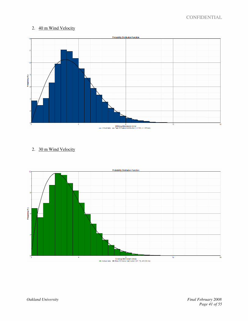
2. 40 m Wind Velocity
2. 30 m Wind Velocity
CONFIDENTIAL
Oakland University Final February 2008
Page 42 of 55
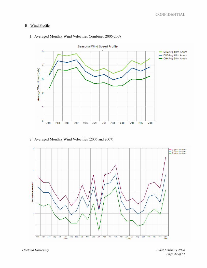
B. Wind Profile
1. Averaged Monthly Wind Velocities Combined 2006-2007
2. Averaged Monthly Wind Velocities (2006 and 2007)
CONFIDENTIAL
Oakland University Final February 2008
Page 43 of 55
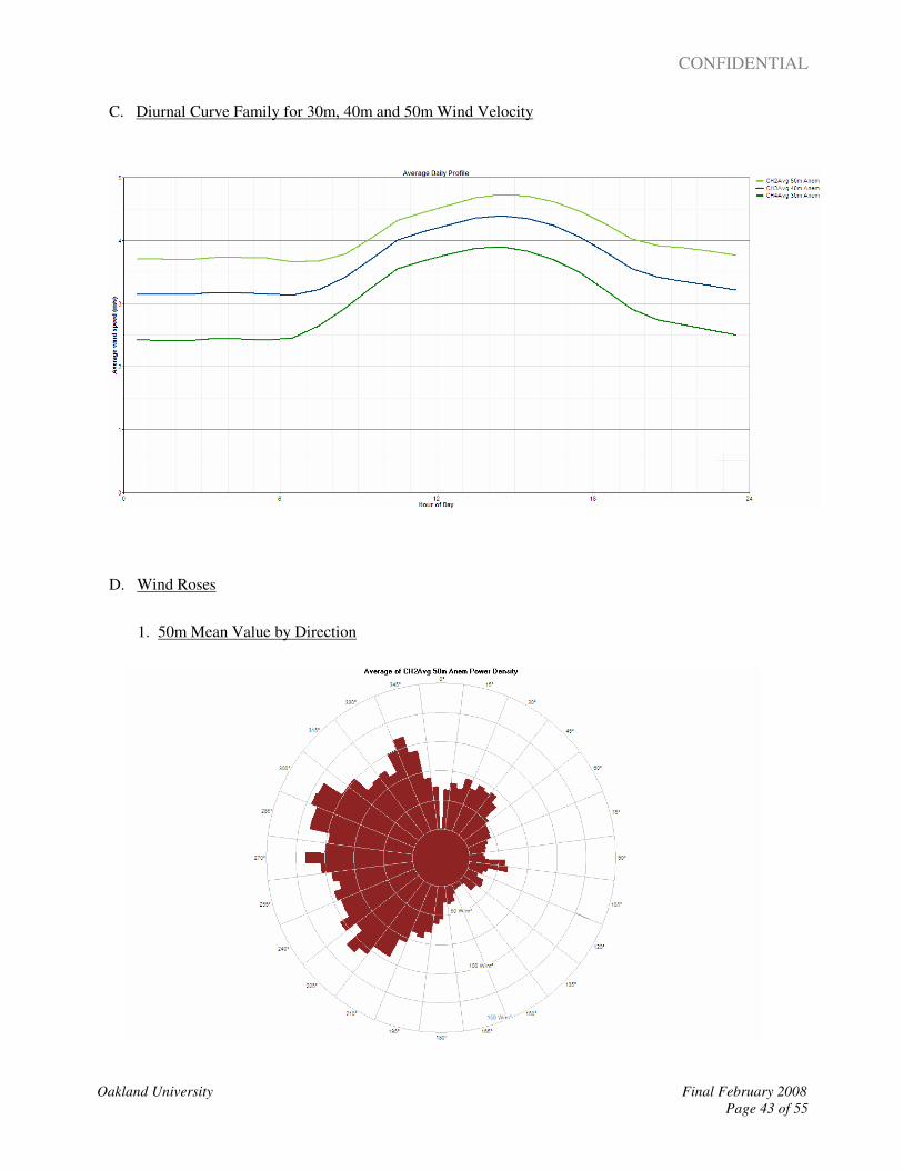
C. Diurnal Curve Family for 30m, 40m and 50m Wind Velocity
D. Wind Roses
1. 50m Mean Value by Direction
CONFIDENTIAL
Oakland University Final February 2008
Page 44 of 55
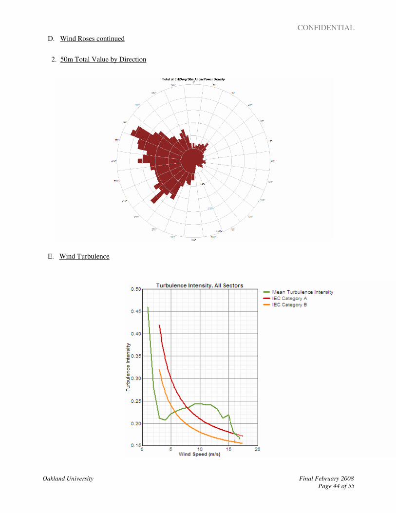
D. Wind Roses continued
2. 50m Total Value by Direction
E. Wind Turbulence
CONFIDENTIAL
Oakland University Final February 2008
Page 45 of 55
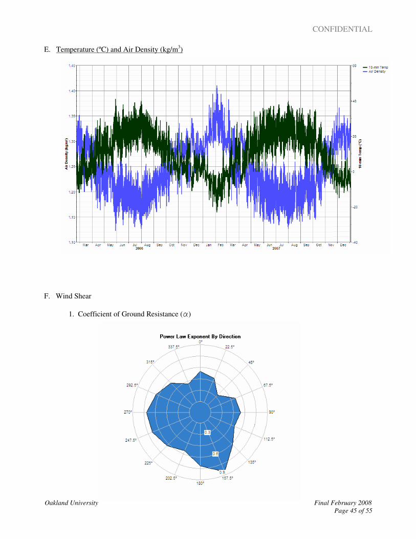
E. Temperature (ºC) and Air Density (kg/m3)
F. Wind Shear
1. Coefficient of Ground Resistance (aaaa)
CONFIDENTIAL
Oakland University Final February 2008
Page 46 of 55
2. Comparison of Power and Logarithmic Law Exponent Vertical Profiles
G. Wind Velocity Time Series
1. 50m Monitored Time Series First Half Calendar 2006
CONFIDENTIAL
Oakland University Final February 2008
Page 47 of 55
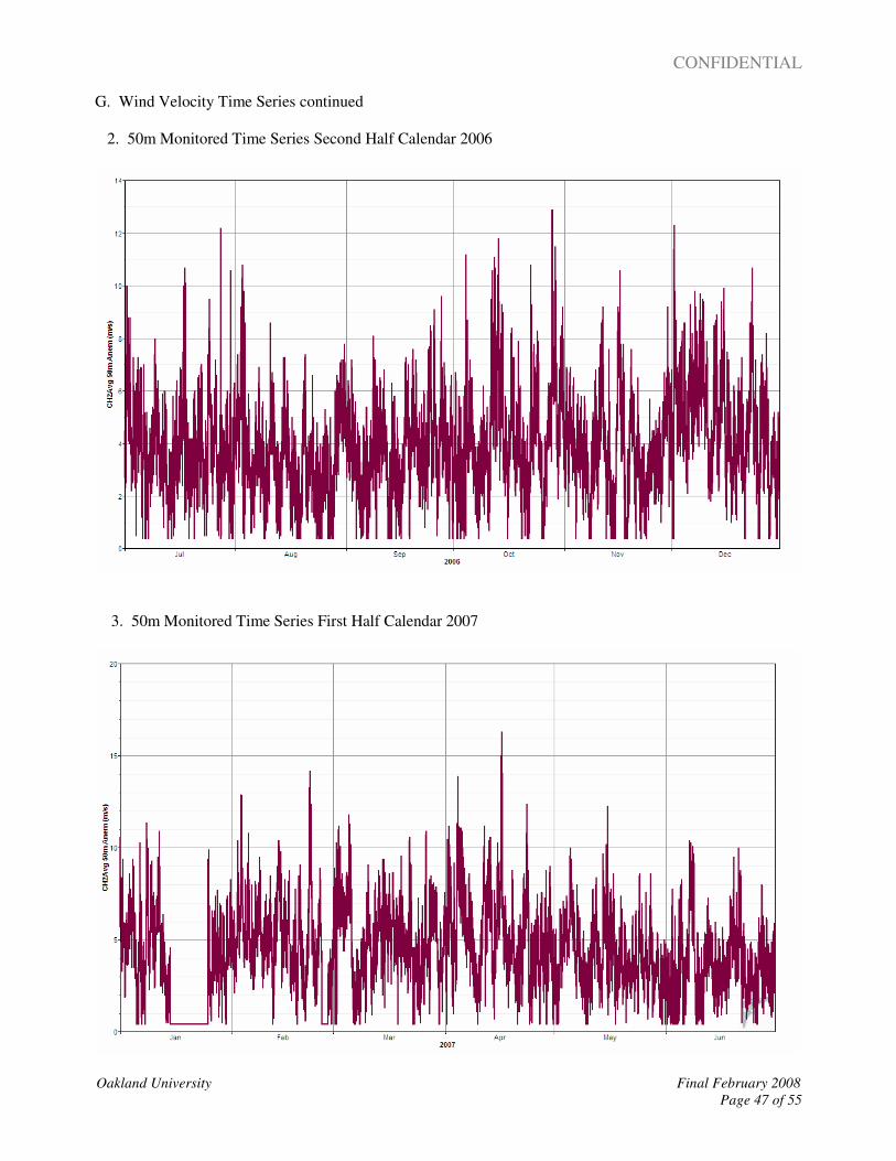
G. Wind Velocity Time Series continued
2. 50m Monitored Time Series Second Half Calendar 2006
3. 50m Monitored Time Series First Half Calendar 2007
CONFIDENTIAL
Oakland University Final February 2008
Page 48 of 55
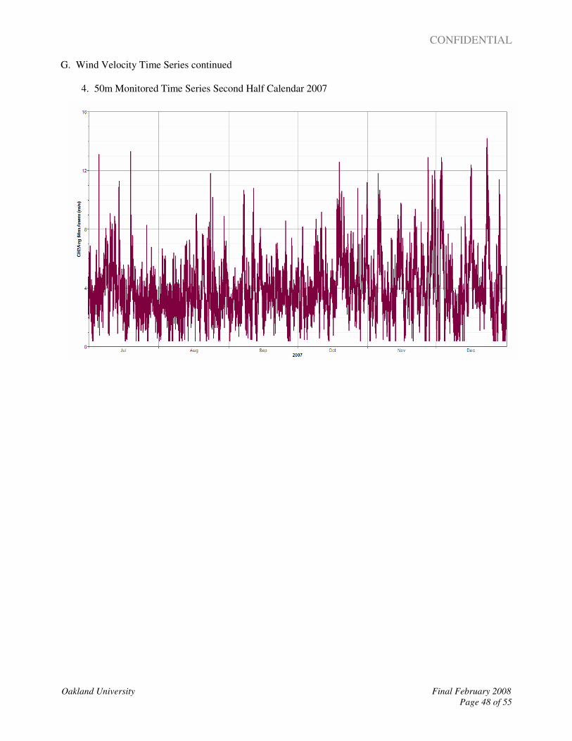
G. Wind Velocity Time Series continued
4. 50m Monitored Time Series Second Half Calendar 2007

CONFIDENTIAL
Oakland University Final February 2008
Page 49 of 55
Section 7
Historical Wind Data, Correlation and Prediction
Historical weather data was compiled from the National Weather Service and Weather
Underground, and NOAA for three general regional reference comparisons. The references
consulted included Detroit Wayne County Metropolitan Airport, Flint Bishop Airport and Pontiac
Airport.
Pontiac Airport was the preferred study reference with obvious proximity to Oakland University
and was chosen to gain a historical perspective on the wind regime.
Eleven year historical data was used for this task. The objective for the correlation defined by
Oakland University was to determine if the wind velocities monitored on Main Campus for the
period February 21, 2006 to December 31, 2007, was weaker, stronger or on average with the
previous years.
The number of graphic curves were limited for readability and clarity.

CONFIDENTIAL
Oakland University Final February 2008
Page 50 of 55
Pontiac Airport
Pontiac Airport is located approximately 16.3 km (10.2 miles) west of Oakland University’s main
campus. The airport runway is at an elevation of approximately 288 m (945 ft) asl. The
meteorological anemometer used at the airport is mounted at an elevation of 3m above ground level.
The elevation of Pontiac Airport is higher than elevation of Oakland’s meteorological tower by
about 15 m (49 ft.) Airport property is level and free of trees, tall buildings, and other obstructions
to wind flow. It is reasonable to state that with respect to wind sheer, the airport will have
considerable less sheer than what is found on the Main Campus.
Wind velocity is measured at Pontiac Airport at only one elevation; therefore, we are not able to
estimate wind shear from measured wind speed observations.
Pontiac Airport and Oakland University
Pontiac Airport (PTK) Oakland University
CONFIDENTIAL
Oakland University Final February 2008
Page 51 of 55
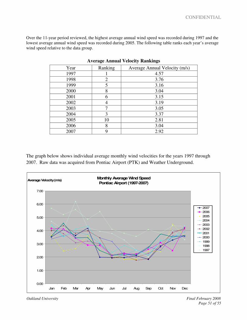
Over the 11-year period reviewed, the highest average annual wind speed was recorded during 1997 and the
lowest average annual wind speed was recorded during 2005. The following table ranks each year’s average
wind speed relative to the data group.
Average Annual Velocity Rankings
The graph below shows individual average monthly wind velocities for the years 1997 through
2007. Raw data was acquired from Pontiac Airport (PTK) and Weather Underground.
Monthly Average Wind Speed
Pontiac Airport (1997-2007)
0.00
1.00
2.00
3.00
4.00
5.00
6.00
7.00
Jan Feb Mar Apr May Jun Jul Aug Sep Oct Nov Dec
Average Velocity (m/s)
2007
2006
2005
2004
2003
2002
2001
2000
1999
1998
1997
Year Ranking Average Annual Velocity (m/s)
1997 1 4.57
1998 2 3.76
1999 5 3.16
2000 8 3.04
2001 6 3.15
2002 4 3.19
2003 7 3.05
2004 3 3.37
2005 10 2.81
2006 8 3.04
2007 9 2.92
CONFIDENTIAL
Oakland University Final February 2008
Page 52 of 55
Monitoring Period Average vs Data Averages (1997-2007)
Pontiac Airport
0.00
0.50
1.00
1.50
2.00
2.50
3.00
3.50
4.00
4.50
Jan Feb Mar Apr May Jun Jul Aug Sep Oct Nov Dec
Average Velocity (m/s)
Potiac (2006-2007)
Pontiac (1997-2007)
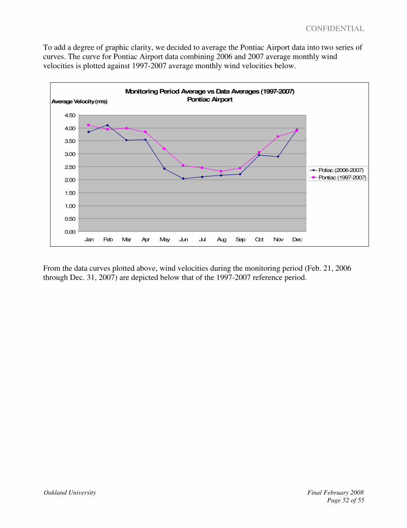
To add a degree of graphic clarity, we decided to average the Pontiac Airport data into two series of
curves. The curve for Pontiac Airport data combining 2006 and 2007 average monthly wind
velocities is plotted against 1997-2007 average monthly wind velocities below.
From the data curves plotted above, wind velocities during the monitoring period (Feb. 21, 2006
through Dec. 31, 2007) are depicted below that of the 1997-2007 reference period.

CONFIDENTIAL
Oakland University Final February 2008
Page 53 of 55
Section 8
Wind Turbine Energy Capture _________________________________________________________________________________________________________________________________________________________________________________________________________________________________________________
Energy capture calculations are preliminary and were performed using energy capture modeling
software for seventeen (17) wind turbine generators at various tower hub height. These turbines
were represented by twelve different manufacturers. The results of these computations served as the
basis for Mr. Jim Leidel’s selection of Request for Quotations (RFQs) recipients all being Original
Equipment Manufacturers (OEM) of wind turbine generators.
The most pragmatic nameplate ratings for generation were chosen to be from 900kW to 2,000kW.
We have narrowed the selection of possible wind turbine units down to three models based on
selection of manufactured tower heights, nameplate ratings, technology, estimated energy capture
and unit availability of installation during the fall of 2008 or spring of 2009.
Tier One List and Preliminary Energy Capture Table
Two additional manufacturers and/or reputable third parties having access to the following turbines
have been contacted. The Request for Quotation has been sent and currently pending replies. The
Tier Two manufacturer pending list and estimates follow.
Tier Two List and Preliminary Energy Capture Table
Notes to Section Tables:
Note (1) Energy capture estimates were taken using synthesized data for 60m, 70m 80, 90m,100m and 110m wind
patterns.
Note (2) Power Law and Logarithmic Law analysis was performed for each model, with the lower estimate being taken.
Note (3) Energy capture projection will require further refinement, estimated projections have a tolerance of ±25%.
Preliminary energy capture estimates will be refined by the engineering departments of the
individual product manufacturer selected by Facilities Management and will be affixed to the
Feasibility Study as addendums upon receipt.
Manufacturer Model Nameplate D rotor
(m) Control
Hub
Height
(m)
Estimated
Energy
Capture
Estimated
MWh/year
AAER 1500-77 1500 kW 77 Pitch 80 18.8 2,474
AWE 54-900 900kW 54 Pitch 75 15.3 1,206
Enercon E82 2000 kW 82 Pitch 108 24.8 4,353
Fuhrlander FL 1500 1500 kW 77 Pitch 115 25.5 3,352
Manufacturer Model Nameplate D rotor
(m) Control
Hub
Height
(m)
Estimated
Energy
Capture
Estimated
MWh/year
AWE 54-900 900kW 54 Pitch 100 24.8 1,955
Nordex S77 1500 kW 77 Pitch 112 24.6 3,233
Vestas V100 2750 kW 100 Pitch 100 32.2 7,756
CONFIDENTIAL
Oakland University Final February 2008
Page 54 of 55
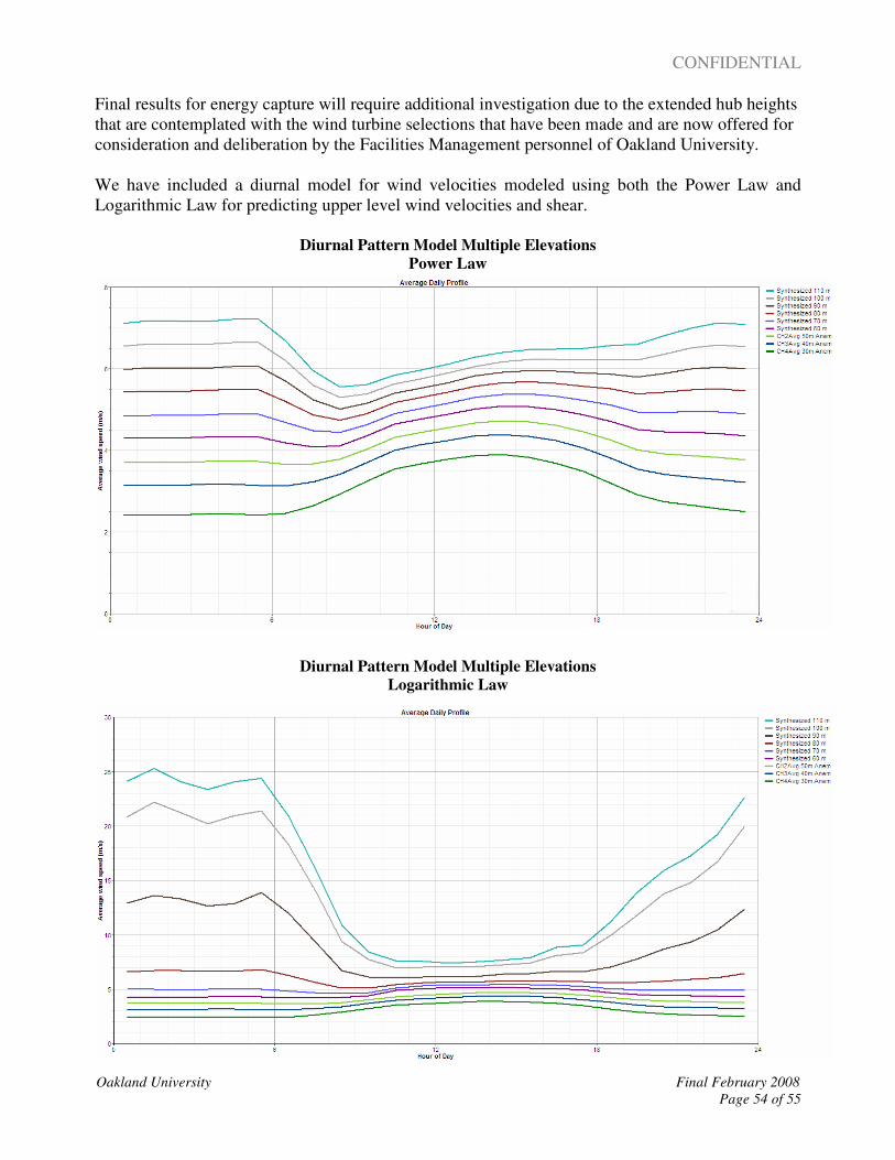
Final results for energy capture will require additional investigation due to the extended hub heights
that are contemplated with the wind turbine selections that have been made and are now offered for
consideration and deliberation by the Facilities Management personnel of Oakland University.
We have included a diurnal model for wind velocities modeled using both the Power Law and
Logarithmic Law for predicting upper level wind velocities and shear.
Diurnal Pattern Model Multiple Elevations
Power Law
Diurnal Pattern Model Multiple Elevations
Logarithmic Law

CONFIDENTIAL
Oakland University Final February 2008
Page 55 of 55
Section 9
Recommendations _________________________________________________________________________________________________________________________________________________________________________________________________________________________________________________
We believe that the wind resource will support wind turbine generation. Although the wind regime
is weak at low elevations, due to increased wind shear factors. The use of higher turbine towers and
the selection of wind turbine generators that have been designed to complement lower wind regimes,
should make this a viable project.
We humbly offer several recommendations for the benefit of Oakland University.
Recommendations:
The wind resource over Oakland University’s Main Campus has a degree of complexity that merits
additional investigation. We suggest that the University consider commissioning a micro-siting
wind map to further assist in determining the final placement location for one or more wind turbine
generators.
Computational fluid dynamic (CFD) software is well suited for this type of investigation. CFD is
used to model complex fluid flow problems for aircraft, missile systems and thermal dynamic. The
objective for the advanced modeling will be determination of highest wind power density
concentrations on Main Campus and at what elevations they are most likely to occur.
Additional validation of higher elevation wind velocities can be accomplished with a Doppler radar
study of a sampling of season weather patterns. The off-site metered data from the meteorological
tower, and the radar data, may be used with the CFD software for more accurate modeling of wind
power density and micro-siting of wind turbine generators.
The individuals that were part of the decision-making team for the above recommendations
included Dr. Patel, Thomas Palermo, and John Wolar.
This Meteorological Tower Data and Compilation report, and recommendations, are submitted to
the Facilities Management Department of Oakland University for prudent consideration.
Respectfully submitted,
John Wolar


![Modelling and simulation of a solar tower power plant...The solar radiation can be computed by the Meteorological Radiation Model (MRM) [2]. As solar tower power plants are mostly](https://img.pdfslide.net/doc/110x75/5f102d8d7e708231d447d476/modelling-and-simulation-of-a-solar-tower-power-plant-the-solar-radiation-can.jpg)