Metering, Monitoring and Targeting - Invest Northern … · 2.0 What is Metering, Monitoring and Targeting ... 3.3 Improved product costing ... 4.5 A system for analysis

Metering, Monitoring and Targeting A best practice guide for businesses in Northern Ireland

2

Invest Northern Ireland Sustainable Development Team T: 028 9069 8868 E: [email protected]

Table of Contents

1.0 Purpose of the Guide . . . . . . . . . . . . . . . . . . . . . . . . . . . . . . . . . . . . . . . . . . . . . . . . . . . . . . . . . . . 4

1.1 Who is this guide for? . . . . . . . . . . . . . . . . . . . . . . . . . . . . . . . . . . . . . . . . . . . . . . . . . . . . . . . . 5

1.2 What is the scope of this guide? . . . . . . . . . . . . . . . . . . . . . . . . . . . . . . . . . . . . . . . . . . . . . . . 5

1.3 How to use this guidance . . . . . . . . . . . . . . . . . . . . . . . . . . . . . . . . . . . . . . . . . . . . . . . . . . . . . 5

1.4 Additional sources of guidance . . . . . . . . . . . . . . . . . . . . . . . . . . . . . . . . . . . . . . . . . . . . . . . . 5

2.0 What is Metering, Monitoring and Targeting (MM&T)? . . . . . . . . . . . . . . . . . . . . . . . . . . . . . . . . 6

2.1 What is monitoring and targeting? . . . . . . . . . . . . . . . . . . . . . . . . . . . . . . . . . . . . . . . . . . . . . . 7

2.2 Is monitoring and targeting complex? . . . . . . . . . . . . . . . . . . . . . . . . . . . . . . . . . . . . . . . . . . . 7

2.3 Is monitoring and targeting easy to implement? . . . . . . . . . . . . . . . . . . . . . . . . . . . . . . . . . . . 7

2.4 Will MM&T save money? . . . . . . . . . . . . . . . . . . . . . . . . . . . . . . . . . . . . . . . . . . . . . . . . . . . . . 7

2.5 Does MM&T require trained or specialist staff input? . . . . . . . . . . . . . . . . . . . . . . . . . . . . . . . . 7

2.6 Is there a significant associated investment cost? . . . . . . . . . . . . . . . . . . . . . . . . . . . . . . . . . . 7

3.0 What are the benefits of MM&T? . . . . . . . . . . . . . . . . . . . . . . . . . . . . . . . . . . . . . . . . . . . . . . . . . 8

3.1 Energy consumption reduction . . . . . . . . . . . . . . . . . . . . . . . . . . . . . . . . . . . . . . . . . . . . . . . . . 9

3.2 How much money will be saved? . . . . . . . . . . . . . . . . . . . . . . . . . . . . . . . . . . . . . . . . . . . . . . . 9

3.3 Improved product costing . . . . . . . . . . . . . . . . . . . . . . . . . . . . . . . . . . . . . . . . . . . . . . . . . . . . 9

3.4 Improved budgeting . . . . . . . . . . . . . . . . . . . . . . . . . . . . . . . . . . . . . . . . . . . . . . . . . . . . . . . . . 9

3.5 Improved planned preventative maintenance . . . . . . . . . . . . . . . . . . . . . . . . . . . . . . . . . . . . . . 9

3.6 Improved product quality . . . . . . . . . . . . . . . . . . . . . . . . . . . . . . . . . . . . . . . . . . . . . . . . . . . . . 9

3.7 Waste reduction . . . . . . . . . . . . . . . . . . . . . . . . . . . . . . . . . . . . . . . . . . . . . . . . . . . . . . . . . . . . 9

4.0 What constitutes an MM&T system? . . . . . . . . . . . . . . . . . . . . . . . . . . . . . . . . . . . . . . . . . . . . . 10

4.1 A system for energy measurement, metering and recording . . . . . . . . . . . . . . . . . . . . . . . . . 11

4.2 A facility for relating energy consumption and production activity . . . . . . . . . . . . . . . . . . . . . 11

4.3 The derivation of standards – what is current performance? . . . . . . . . . . . . . . . . . . . . . . . . . 11

4.4 Comparing performance . . . . . . . . . . . . . . . . . . . . . . . . . . . . . . . . . . . . . . . . . . . . . . . . . . . . . 11

4.5 A system for analysis – how is performance assessed and variance measured, what does it mean? . . . . . . . . . . . . . . . . . . . . . . . . . . . . . . . . . . . . . . . . . . . . . . . . . . . . . . . . 11

4.6 A system for reporting – how is the information conveyed and to whom? . . . . . . . . . . . . . . 11

4.7 A system for improvement- how is the information acted upon?. . . . . . . . . . . . . . . . . . . . . . 12

5.0 Planning for the implementation of an MM&T system . . . . . . . . . . . . . . . . . . . . . . . . . . . . . . . 13

5.1 Establishing Cost Centres (Energy Accounting Centres) . . . . . . . . . . . . . . . . . . . . . . . . . . . . 14

5.2 Who is best able to determine the constitution cost centres? . . . . . . . . . . . . . . . . . . . . . . . . 14

5.3 What basis for energy and production activity should be selected? . . . . . . . . . . . . . . . . . . . 14

5.4 Will additional metering be required? . . . . . . . . . . . . . . . . . . . . . . . . . . . . . . . . . . . . . . . . . . . 14

3

5.5 What data collection procedures will be required? . . . . . . . . . . . . . . . . . . . . . . . . . . . . . . . . 15

5.6 Is management commitment essential? . . . . . . . . . . . . . . . . . . . . . . . . . . . . . . . . . . . . . . . . . 15

5.7 Preparing a business plan for MM&T . . . . . . . . . . . . . . . . . . . . . . . . . . . . . . . . . . . . . . . . . . . 15

6.0 Cost Centres and Specific Energy Consumption (SEC) . . . . . . . . . . . . . . . . . . . . . . . . . . . . . . 16

6.1 What basis should be used for SEC? . . . . . . . . . . . . . . . . . . . . . . . . . . . . . . . . . . . . . . . . . . . 17

6.2 What data frequency is required for my cost centres and SEC? . . . . . . . . . . . . . . . . . . . . . . 18

6.3 What if I produce different products on the same machines? . . . . . . . . . . . . . . . . . . . . . . . . 18

7.0 Meter selection . . . . . . . . . . . . . . . . . . . . . . . . . . . . . . . . . . . . . . . . . . . . . . . . . . . . . . . . . . . . . . 19

7.1 What is the Measuring Instruments Directive? . . . . . . . . . . . . . . . . . . . . . . . . . . . . . . . . . . . . 20

7.2 Criteria for meter selection . . . . . . . . . . . . . . . . . . . . . . . . . . . . . . . . . . . . . . . . . . . . . . . . . . . 20

7.3 Turndown ratio . . . . . . . . . . . . . . . . . . . . . . . . . . . . . . . . . . . . . . . . . . . . . . . . . . . . . . . . . . . . 20

7.4 Accuracy . . . . . . . . . . . . . . . . . . . . . . . . . . . . . . . . . . . . . . . . . . . . . . . . . . . . . . . . . . . . . . . . . 20

7.5 Repeatability . . . . . . . . . . . . . . . . . . . . . . . . . . . . . . . . . . . . . . . . . . . . . . . . . . . . . . . . . . . . . . 20

7.6 What does Modbus compatible mean? . . . . . . . . . . . . . . . . . . . . . . . . . . . . . . . . . . . . . . . . . 20

7.7 What meters do I need? . . . . . . . . . . . . . . . . . . . . . . . . . . . . . . . . . . . . . . . . . . . . . . . . . . . . . 20

8.0 Operating the MM&T system . . . . . . . . . . . . . . . . . . . . . . . . . . . . . . . . . . . . . . . . . . . . . . . . . . . 21

8.1 Setting standards . . . . . . . . . . . . . . . . . . . . . . . . . . . . . . . . . . . . . . . . . . . . . . . . . . . . . . . . . . 22

8.2 How is MM&T used to improve control and reduce energy consumption? . . . . . . . . . . . . . . 22

9.0 Calculating Standards . . . . . . . . . . . . . . . . . . . . . . . . . . . . . . . . . . . . . . . . . . . . . . . . . . . . . . . . . 24

9.1 Specific energy consumption vs. production . . . . . . . . . . . . . . . . . . . . . . . . . . . . . . . . . . . . . 27

9.2 Why is volume related SEC important? . . . . . . . . . . . . . . . . . . . . . . . . . . . . . . . . . . . . . . . . . 28

9.3 Regression analysis . . . . . . . . . . . . . . . . . . . . . . . . . . . . . . . . . . . . . . . . . . . . . . . . . . . . . . . . 28

9.4 Alternative solutions for target setting. . . . . . . . . . . . . . . . . . . . . . . . . . . . . . . . . . . . . . . . . . . 28

10.0 Evaluating Performance change . . . . . . . . . . . . . . . . . . . . . . . . . . . . . . . . . . . . . . . . . . . . . . . . 31

10.1 Identifying trends . . . . . . . . . . . . . . . . . . . . . . . . . . . . . . . . . . . . . . . . . . . . . . . . . . . . . . . . . . 32

10.2 Improving consistency and accuracy . . . . . . . . . . . . . . . . . . . . . . . . . . . . . . . . . . . . . . . . . . 32

11.0 CUSUM (Cumulative sum of errors) Techniques . . . . . . . . . . . . . . . . . . . . . . . . . . . . . . . . . . . 34

11.1 CUSUM convention . . . . . . . . . . . . . . . . . . . . . . . . . . . . . . . . . . . . . . . . . . . . . . . . . . . . . . . . 38

11.2 Caution with CUSUM . . . . . . . . . . . . . . . . . . . . . . . . . . . . . . . . . . . . . . . . . . . . . . . . . . . . . . . 38

12.0 Feedback and reporting . . . . . . . . . . . . . . . . . . . . . . . . . . . . . . . . . . . . . . . . . . . . . . . . . . . . . . . 39

13.0 How do you assess building energy performance? . . . . . . . . . . . . . . . . . . . . . . . . . . . . . . . . . 41

13.1 Degree days . . . . . . . . . . . . . . . . . . . . . . . . . . . . . . . . . . . . . . . . . . . . . . . . . . . . . . . . . . . . . . 42

13.2 Where do I get degree day figures from? . . . . . . . . . . . . . . . . . . . . . . . . . . . . . . . . . . . . . . . 42

13.3 Degree Days work in practice? . . . . . . . . . . . . . . . . . . . . . . . . . . . . . . . . . . . . . . . . . . . . . . . 45

13.4 Using the CUSUM analysis to verify trends . . . . . . . . . . . . . . . . . . . . . . . . . . . . . . . . . . . . . . 46

14.0 Energy Performance in Buildings - Key Legislative Changes . . . . . . . . . . . . . . . . . . . . . . . . 47

14.1 Energy performance certificates and energy benchmarking . . . . . . . . . . . . . . . . . . . . . . . . . 48

14.2 Building Logbooks . . . . . . . . . . . . . . . . . . . . . . . . . . . . . . . . . . . . . . . . . . . . . . . . . . . . . . . . . 48

14.3 What is in a Building Logbook . . . . . . . . . . . . . . . . . . . . . . . . . . . . . . . . . . . . . . . . . . . . . . . . 48

14.4 Energy Savings Opportunity Scheme (ESOS) . . . . . . . . . . . . . . . . . . . . . . . . . . . . . . . . . . . . 49

15.0 Other Useful Reading . . . . . . . . . . . . . . . . . . . . . . . . . . . . . . . . . . . . . . . . . . . . . . . . . . . . . . . . . 50

4

1.0 Purpose of the Guide1.1 Who is this guide for? . . . . . . . . . . . . . . . . . . . . . . . . . . . . . . . . . . . . . . . . . . . . . . . . . . . . 5

1.2 What is the scope of this guide? . . . . . . . . . . . . . . . . . . . . . . . . . . . . . . . . . . . . . . . . . . . . 5

1.3 How to use this guidance . . . . . . . . . . . . . . . . . . . . . . . . . . . . . . . . . . . . . . . . . . . . . . . . . 5

1.4 Additional sources of guidance . . . . . . . . . . . . . . . . . . . . . . . . . . . . . . . . . . . . . . . . . . . . . 5

5

All businesses consume or produce energy - understanding how much energy we use, for what purpose, and how we exercise control over energy consumption and cost, is vital for environmental and commercial security.

This guide explains, concisely, the basic guiding principles relating to the conception, development and procurement of metering, monitoring and targeting systems (MM&T).

1.1 Who is this guide for? This guide is primarily intended for companies who currently do not use MM&T, but it is also relevant to those who already operate MM&T systems for building energy consumption or for industrial activities.

1.2 What is the scope of this guide? This guide covers aspects of concept, development and the practical operation of an MM&T system. The guide does not cover specific installations or products other than by way of example.

It provides a detailed explanation of some of the fundamental aspects of MM&T installation and operation and includes the following:

• The basic concepts

• The system requirements

• The benefits

• Operational considerations

1.3 How to use this guidance This guide is split into stand-alone sections that may be read in isolation or in sequence. If read in sequence the document follows the procedure that should be adopted to develop a successful MM&T project. However, guidance on specific subject matters may be obtained by reference to the relevant section.

1.4 Additional sources of guidance This guide contains a list of additional sources of guidance.

Purpose of the Guide

6

2.1 What is monitoring and targeting? . . . . . . . . . . . . . . . . . . . . . . . . . . . . . . . . . . . . . . . . . . . 7

2.2 Is monitoring and targeting complex? . . . . . . . . . . . . . . . . . . . . . . . . . . . . . . . . . . . . . . . . 7

2.3 Is monitoring and targeting easy to implement? . . . . . . . . . . . . . . . . . . . . . . . . . . . . . . . . 7

2.4 Will MM&T save money? . . . . . . . . . . . . . . . . . . . . . . . . . . . . . . . . . . . . . . . . . . . . . . . . . . 7

2.5 Does MM&T require trained or specialist staff input? . . . . . . . . . . . . . . . . . . . . . . . . . . . . 7

2.6 Is there a significant associated investment cost? . . . . . . . . . . . . . . . . . . . . . . . . . . . . . . 7

2.0 What is Metering, Monitoring and Targeting (MM&T)?

7

2.1 What is monitoring and targeting?Monitoring and targeting is a term used to describe a range of management techniques employed to improve understanding of how energy is consumed and business costs are evolved. MM&T is a management system for controlling energy consumption and cost. It allows performance measurement with a greater degree of accuracy and can be used to improve accountability, quality and profitability.

If, specifically, your process systems performance deteriorates, you will be faced with increasing costs and perhaps even product quality or productivity issues.

It is therefore prudent to manage these systems effectively. To manage any system effectively you must have knowledge of its performance.

An excellent analogy is the fuel consumption of a car. A poorly maintained car with worn engine, under-inflated tyres and poor carburettor set up will have poor fuel performance.

Recognising poor fuel performance with fluctuating petrol prices is difficult. But if you keep a simple record of fuel consumed and mileage travelled you may well be able to determine performance. In addition:

• You will be able to identify performance loss quickly.

• You will be able to predict the fuel consumption for a specific journey.

• You may care to drive more sensibly when you are able to see clearly how much fuel you use.

• You may be able to predict the need for service or tune up. (PPM Planned Preventive Maintenance).

• You will be able to see the benefit of tune up.

• You may make allowances or corrections depending on the type of driving you are doing (motorway or urban).

• You could establish whether your Ford Escort compares favourably with the Fords published figures. (Benchmarking).

• You could set your own fuel performance targets to be achieved by careful driving and good car maintenance. (Internal Benchmarking).

The same concepts are true (if not more so) for any fuel or power consuming processes. The process of monitoring and targeting is very similar and can be as elaborate or as simple as required to allow your complete understanding of system performance.

2.2 Is Monitoring and targeting complex?Monitoring and targeting can be as simple as routinely taking a meter reading and checking consumption against production. Or it can be a complex multivariable process based analytical tool.

Contrary to common belief a useful M&T (monitoring and targeting) system can be extremely simple. It is really not about how complex the system is, it is about how appropriate the system is.

2.3 Is monitoring and targeting easy to implement?Yes it is a simple management procedure requiring the collection and analysis of energy and production data. In some cases the process can be largely automated using data collection and analysis software.

2.4 Will MM&T save money?Yes - If you do not meter, then you do not measure and therefore you cannot manage energy effectively.

2.5 Does MM&T require trained or specialist staff input?Generally not, although some knowledge of process and spreadsheets are useful. MM&T (metering, monitoring and targeting) is really the application of techniques that allow you to carry out existing business and process function with improved control and awareness of energy consumption and cost.

2.6 Is there a significant associated investment cost?Not necessarily. MM&T can be implemented with relatively little cost (sometimes no capital cost). Where it is necessary to purchase additional metering, there are additional costs.

There are costs associated with managing energy. These costs arise from labour engaged in collecting, analysing and presenting data. However, these costs may be relatively small when compared to the prospective savings potential.

What is Metering, Monitoring and Targeting (MM&T)?

8

3.1 Energy consumption reduction . . . . . . . . . . . . . . . . . . . . . . . . . . . . . . . . . . . . . . . . . . . . . 9

3.2 How much money will be saved? . . . . . . . . . . . . . . . . . . . . . . . . . . . . . . . . . . . . . . . . . . . 9

3.3 Improved product costing . . . . . . . . . . . . . . . . . . . . . . . . . . . . . . . . . . . . . . . . . . . . . . . . . 9

3.4 Improved budgeting . . . . . . . . . . . . . . . . . . . . . . . . . . . . . . . . . . . . . . . . . . . . . . . . . . . . . . 9

3.5 Improved planned preventative maintenance . . . . . . . . . . . . . . . . . . . . . . . . . . . . . . . . . . 9

3.6 Improved product quality . . . . . . . . . . . . . . . . . . . . . . . . . . . . . . . . . . . . . . . . . . . . . . . . . . 9

3.7 Waste reduction . . . . . . . . . . . . . . . . . . . . . . . . . . . . . . . . . . . . . . . . . . . . . . . . . . . . . . . . . 9

3.0 What are the benefits of MM&T ?

9

3.1 Energy consumption reductionThe obvious benefit is controlling the use of energy. However MM&T can be used for much more and can be used as a performance diagnostic tool for a process or for specific elements of a process. For example, in the context of a boiler, or a steam system this management tool can be adapted and used quite creatively to allow continuous performance analyses.

3.2 How much money will be savedThis is entirely dependent on the process, the site, the existing degree of control and so on. However, for most industrial sites the expectation might be 5% savings potential from MM&T alone.

3.3 Improved product costingThe value of energy as part of the product cost can be assessed and understood using MM&T. If you understand the cost you are more likely to be in a position to control the cost. This is particularly true for variable production runs. It is usually evident that economies of scale exist in most production activities. MM&T can help identify and accurately quantify these economies of scale.

There are two distinct benefits. Firstly, production can be scheduled to achieve the best specific energy consumption and lowest cost per unit production. Secondly, the cost to customer can be passed on accurately and short run product priced with accuracy.

3.4 Improved budgetingThe relationship between production and energy can be established, energy and cost forecasts can be reliably derived for planned production activities.

3.5 Improved planned preventative maintenanceThe examination of specific consumption trends can tell a lot about the performance and efficiency. Just as increased fuel consumption in the example of the car can be used to detect the need for a tune up, an MM&T system can be used to detect deteriorating plant performance.

3.6 Improved product qualityUncontrolled or variable energy performance often results from poor system control with similar adverse implications for quality. A spin off from effective energy management is improved process control and improved production or product quality - It is not a direct effect of MM&T but a secondary benefit.

3.7 Waste reductionAn MM&T system aids the cost of wasted production to be evaluated, understood and hopefully avoided. Waste costs twice in energy terms. The original energy consumed and the energy consumed to make the replacement product.

What are the benefits of MM&T?

10

4.1 A system for energy measurement, metering and recording . . . . . . . . . . . . . . . . . . . . . . 11

4.2 A facility for relating energy consumption and production activity . . . . . . . . . . . . . . . . . 11

4.3 The derivation of standards – what is current performance? . . . . . . . . . . . . . . . . . . . . . 11

4.4 Comparing performance . . . . . . . . . . . . . . . . . . . . . . . . . . . . . . . . . . . . . . . . . . . . . . . . . 11

4.5 A system for analysis – how is performance assessed and variance measured, what does it mean? . . . . . . . . . . . . . . . . . . . . . . . . . . . . . . . . . . . . . . . . . . . . . . . . . . . . . 11

4.6 A system for reporting – how is the information conveyed and to whom? . . . . . . . . . . . 11

4.7 A system for improvement - how is the information acted upon? . . . . . . . . . . . . . . . . . . 12

4.0 What constitutes an MM&T system?

11

4.1 A system for energy measurement, metering and recordingMetering is an essential prerequisite for effective monitoring and targeting. Energy saving measures may only be identified and implemented if energy performance is understood. To do this metering is required.

The principal barrier to expenditure on metering is the apparent lack of tangible payback. In fact metering provides the evidence to prioritise and justify the installation of energy efficiency improvements.

4.2 A facility for relating energy consumption and production activityTo understand how production activity is related to energy consumption and cost, it is necessary to measure production output.

The energy consumption per unit production is called the specific energy consumption or SEC. The SEC might well vary with production volume - becoming less with large volume production (economies of scale) and often typically increasing with short production runs.

The basis for quantifying production varies from site to site and production activity to production activity. Many companies produce a range of products from similar feed stocks and there may be some considerable variation in specific energy consumption. It may be necessary to develop a series of product specific indicators or develop an SEC that uses raw materials as a measurement basis.

MM&T is routinely used to record and examine the performance of buildings and in that specific circumstance the SEC might vary with external air temperature, occupancy and other variables.

In some cases it may be necessary to develop relatively complex relationships if the consumption patterns are to be understood. However, wherever practical, the least complex and simplest relationships usually work best.

4.3 The derivation of standards – what is current performance?To evaluate any improvement in control, and variation in SEC or cost, the current performance has to be understood. Since the SEC may vary with production volume, temperature or some other variable, the current performance and the performance relationship must be understood.

The derivation of target data and the analysis of that data is explained in this guide.

It is self evident that unless there is a mass of historical data, then the ongoing comparison of performance cannot be made until sufficient “current performance data” is assembled. There are two possible solutions:

• Sufficient historical data is available and can be analysed to set a target.

or

• The system must be operated and used initially just to collect data to allow analysis and the derivation of a target.

4.4 Comparing performanceComparison is usually straight forward and visual comparison of data is often sufficient to allow comprehension of the energy trend and cost and ultimately allow action for control.

In some more complex arrangements where an MM&T system is used to monitor specific plant or process, it is useful to develop a statistical protocol for analysis that allows rapid trend analysis, alarm setting and provide easily understood data analysis.

In most cases a simple relationship between production and consumption can be established and used for the purposes of comparison. This guide explains several basic techniques, and provides some worked examples.

4.5 A system for analysis – how is performance assessed and variance measured, what does it mean?The use of CUSUM techniques (Cumulative Sum of Errors from target) is a simple but particularly useful way of comparing performance when there is a scale related variation in SEC. The CUSUM technique allows quick, accurate trend information to be determined and can be accomplished very simply using basic spreadsheet tools.

The CUSUM technique may be used to rapidly analyse large and complex data sets - and vital trends.

A more detailed explanation is given in this guide.

4.6 A system for reporting – how is the information conveyed and to whom?Analysing performance is meaningless unless the information is acted upon. Even if the sole purpose of the data collection is to check invoices or some equally simple arrangement, the information is worthless unless it is collated, presented and action is taken.

A formal reporting system is therefore required. This might take the form of a straightforward performance or feedback report that is delivered to individuals that have control over the process, heating or other controlled system.

What constitutes an MM&T system?

12

What constitutes an MM&T system?

4.7 A system for improvement – how is the information acted upon?There is little point in having a control system without feedback and error correction - the analogy of the car is ideal once again. If the fuel consumption is consistently poor then the driver may have to service the vehicle, adjust driving style or make improvements to the process e.g. remove items stored unnecessarily in the boot, check tyre pressures, etc.

13

5.0 Planning for the implementation of an MM&T system5.1 Establishing Cost Centres (Energy Accounting Centres) . . . . . . . . . . . . . . . . . . . . . . . . . 14

5.2 Who is best able to determine the constitution cost centres? . . . . . . . . . . . . . . . . . . . . 14

5.3 What basis for energy and production activity should be selected? . . . . . . . . . . . . . . . . 14

5.4 Will additional metering be required? . . . . . . . . . . . . . . . . . . . . . . . . . . . . . . . . . . . . . . . 14

5.5 What data collection procedures will be required? . . . . . . . . . . . . . . . . . . . . . . . . . . . . . 14

5.6 Is management commitment essential? . . . . . . . . . . . . . . . . . . . . . . . . . . . . . . . . . . . . . 15

5.7 Preparing a business plan for MM&T . . . . . . . . . . . . . . . . . . . . . . . . . . . . . . . . . . . . . . . . 15

14

5.1 Establishing Cost Centres (Energy Accounting Centres)MM&T will be used primarily to ascertain the energy consumption associated with a production activity or building. It is important to establish cost centres. A cost centre is an area of business activity, process or plant that can be metered effectively and where there is opportunity to manage and reduce energy consumption.

Cost centres might be determined geographically - a good example would be a district heating system where individual buildings are metered. The energy flow to each building would be monitored (with or without line losses) and the boiler operation might equally constitute a cost centre. In this way the individual building performance, line losses and the boiler house efficiency might all be monitored and consequently managed.

Likewise where separate processes are conducted in different buildings, e.g. rubber mixing and tyre moulding, and it is relatively easy to separately meter and monitor these processes individually. Cost centres might be determined on existing adopted accountancy bases e.g. the weld shop or the paint shop.

It is more difficult when the process stages are contiguous or there are multiple processes in one building (as often is the case). However if a methodical approach is adopted and in house process knowledge is used, an acceptable compromise will almost always be determined.

The important issue is to create a system that provides useful measurement of operational aspects over which you might be able to exercise cost effective control.

These might be:

• process activities (packing and finishing)

• geographical areas (South side production area)

• specific systems (the steam distribution system or boiler house)

• plant items (the boilers or indeed a specific boiler)

Creating a useful MM&T system will require some careful survey and initial analysis of the energy consumption, consumption patterns and production activities.

5.2 Who is best able to determine the constitution cost centres?In developing an MM&T system you could solicit advice from a consultant experienced in the development of MM&T systems. However, it is unlikely that an external consultant or MM&T supplier will have the detailed business knowledge required to establish an optimal solution. An external consultant will, however, be able to explain and define relevant analysis methods.

Cost centres are best developed internally - where practical these should be independently metered so that the energy performance can be ring fenced. Often, however it is not possible to arrange for discrete separation and some compromise is required.

5.3 What basis for energy and production activity should be selected?In selecting cost centres it is also important to consider the Specific Energy Consumption indicators Key Performance Indicators (KPI’s) that will be derived – because it is useful to determine clear and easily used, trended Specific Energy Consumption indicators.

Remember that the SEC is a measure of energy per unit product (or similar). In some cases compromise over exact geographical or process stage delineation will allow a far superior SEC to be more easily collected.

Choosing SEC and the basis for deriving SEC is addressed in the following guide section.

5.4 Will additional metering be required?Yes, because most sites in the UK will only have the utility company’s service meter. The accuracy of the meter should be good and there is a legal duty of care for metering to be accurate and within +/-2% (gas) and +2.5% to 3.5% (electricity). Some 93% of meters are generally within these limits. However if you are spending £50,000 on electricity each year the error could be worth as much as £1,750.

Having identified cost centres it will be necessary to meter these in order to provide a basis for an energy/production relationship.

Planning for the implementation of an MM&T system

15

Notwithstanding the Government’s ‘Smart’ metering programme (which will affect domestic and small commercial users) larger sites will be equipped with ‘Smart’ or advanced utility metering by 2019 allowing full data download. However, the installation of client owned sub metering is a vital part of understanding the breakdown of energy use.

For each cost centre the requirement for metering should be assessed. Metering is addressed in a following section of this guide.

5.5 What data collection procedures will be required?Clearly the meters must be read. Meter reading gives rise to the most difficulty in data analysis. Automatic data collection is far superior to manual collection because the “time of reading” errors can largely be eliminated.

Manual meter reading is acceptable but may be time consuming, depending on the number of meters. Sometimes manual data collection can be irregular or introduce meter reading errors.

Of course the energy or water consumed is only one half of the equation. Accurate energy metering is pointless if the production related activity cannot be measured. Likewise then a means of measuring production must be determined.

Data must be collected regularly, at the same time each day, week or whatever the metering period selected so as to provide comparative intervals of energy and production data.

5.6 Is management commitment essential?Yes, senior management backing and support are required. This is important because the performance of cost centres or buildings will be examined and there must be a commitment to act on the information distilled from the MM&T process.

It is important to understand that MM&T is a management diagnostic system and it requires management input to affect an outcome - MM&T is not a passive system and the managerial structure and staff accountability are a key component of the system architecture.

Senior management commitment is required to support and underwrite the project. Local or cost centre management is required to review and determine the cause of performance variation and provide rectification or control.

5.7 Preparing a business plan for MM&TThere is a cost associated with providing and operating an MM&T system and therefore to implement an MM&T system, a structured development and implementation plan is usually required.

− The potential costs and savings have to be identified.

− The concept must be sold to senior management.

− The methodology and timescale for implementation must be determined.

− The functional and operational requirements of a system must have been established.

− The staffing and skill requirements assessed.

The costs arise, amongst other things, from:

− The level to which monitoring and targeting is exercised (keep it simple)

− Additional meter requirements

− Data collection (time if the system is not automated)

− Analysis requirements (this can also be automated)

− The actual implementation and day to day operation

A balance is required to ensure that the cost of operating the MM&T system does not exceed the potential benefit. Clearly it would be nonsensical to measure monitor and target every aspect of one business or production activity.

Planning for the implementation of an MM&T system

16

6.1 What basis should be used for SEC ? . . . . . . . . . . . . . . . . . . . . . . . . . . . . . . . . . . . . . . . 17

6.2 What data frequency is required for my cost centres and SEC? . . . . . . . . . . . . . . . . . . . 18

6.3 What if I produce different products on the same machines? . . . . . . . . . . . . . . . . . . . . . 18

6.0 Cost Centres and Specific Energy Consumption (SEC)

17

6.1 What basis should be used for SEC?MM&T is generally used to trend performance, so repeatability is more relevant than accuracy (this is explained further within metering section).

The cost centres should be first determined – this is a fundamental consideration of any MM&T system. Refer to the preceding guide section.

Explaining the nature of cost centres and the selection of SEC is important and best explained by the following example:

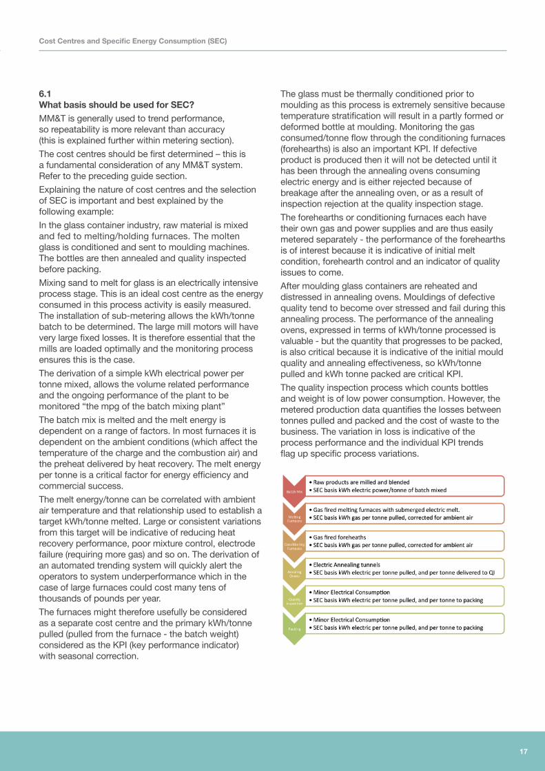
In the glass container industry, raw material is mixed and fed to melting/holding furnaces. The molten glass is conditioned and sent to moulding machines. The bottles are then annealed and quality inspected before packing.

Mixing sand to melt for glass is an electrically intensive process stage. This is an ideal cost centre as the energy consumed in this process activity is easily measured. The installation of sub-metering allows the kWh/tonne batch to be determined. The large mill motors will have very large fixed losses. It is therefore essential that the mills are loaded optimally and the monitoring process ensures this is the case.

The derivation of a simple kWh electrical power per tonne mixed, allows the volume related performance and the ongoing performance of the plant to be monitored “the mpg of the batch mixing plant”

The batch mix is melted and the melt energy is dependent on a range of factors. In most furnaces it is dependent on the ambient conditions (which affect the temperature of the charge and the combustion air) and the preheat delivered by heat recovery. The melt energy per tonne is a critical factor for energy efficiency and commercial success.

The melt energy/tonne can be correlated with ambient air temperature and that relationship used to establish a target kWh/tonne melted. Large or consistent variations from this target will be indicative of reducing heat recovery performance, poor mixture control, electrode failure (requiring more gas) and so on. The derivation of an automated trending system will quickly alert the operators to system underperformance which in the case of large furnaces could cost many tens of thousands of pounds per year.

The furnaces might therefore usefully be considered as a separate cost centre and the primary kWh/tonne pulled (pulled from the furnace - the batch weight) considered as the KPI (key performance indicator) with seasonal correction.

The glass must be thermally conditioned prior to moulding as this process is extremely sensitive because temperature stratification will result in a partly formed or deformed bottle at moulding. Monitoring the gas consumed/tonne flow through the conditioning furnaces (forehearths) is also an important KPI. If defective product is produced then it will not be detected until it has been through the annealing ovens consuming electric energy and is either rejected because of breakage after the annealing oven, or as a result of inspection rejection at the quality inspection stage.

The forehearths or conditioning furnaces each have their own gas and power supplies and are thus easily metered separately - the performance of the forehearths is of interest because it is indicative of initial melt condition, forehearth control and an indicator of quality issues to come.

After moulding glass containers are reheated and distressed in annealing ovens. Mouldings of defective quality tend to become over stressed and fail during this annealing process. The performance of the annealing ovens, expressed in terms of kWh/tonne processed is valuable - but the quantity that progresses to be packed, is also critical because it is indicative of the initial mould quality and annealing effectiveness, so kWh/tonne pulled and kWh tonne packed are critical KPI.

The quality inspection process which counts bottles and weight is of low power consumption. However, the metered production data quantifies the losses between tonnes pulled and packed and the cost of waste to the business. The variation in loss is indicative of the process performance and the individual KPI trends flag up specific process variations.

Cost Centres and Specific Energy Consumption (SEC)

18

Cost Centres and Specific Energy Consumption (SEC)

With some relatively simple metering and process quantification, significant insight into the energy and correct process performance can be established.

In practice, the operation of specific plant might be monitored in more detail (again for example), the air flows to the forehearths might be monitored and the correlation between quality or gas consumed would be established.

The preceding example illustrates how cost centres and SEC may be established. These indicators allow analysis of the different processes, process stages and may be used to gauge process control as well as simply keeping track of energy and cost.

By splitting the processes down into logical cost centres (EAC) with appropriate KPI the opportunity for improved management then arises.

Again by way of an example, if the ratio of tonnes glass bottles packed to tonnes melted starts to fall whilst the forehearth gas/tonne produced rises it might logically be assumed that the bottle rejection or break rate has increased, and because the overall gas/tonne has increased this might be an initial molten glass quality or conditioning issue. A decrease in gas consumption might prompt the same investigation. Regardless, the variation and any trend are used to prompt investigation and resolution before any major technical or commercial damage is done.

Specific Energy Consumption Indicators are usually Key Performance Indicators of kWh/unit raw material or kWh/unit finished component or kWh/degree day for a buildings energy consumption. In some circumstances however it might be necessary to relate kWh to hours of production time or some other less tangible measure of production activity. For most industries however there are usually some good credible KPI’s.

6.2 What data frequency is required for my cost centres and SEC?The frequency of data measurement depends entirely on the likely variation in consumption of the processes and what is to be achieved with the data.

If the data is being used to trend overall kWh/kg or kWh/unit of production over a long time frame to determine any drift in performance, then a longer time frame between measurements is appropriate - a daily consumption or weekly consumption might suit.

If, however, the data is being used to say examine compressor performance and the suitability of sequence control, then data collection might have to be every minute - just for example.

6.3 What if I produce different products on the same machines?If for example you were logging a textile conditioning process and you switched from a grade 1 cotton to grade 12 cotton then it would be appropriate to MM&T these processes separately.

The same would be true for any other industry whether it be castings, injection moulding, glass containers and so on.

Break it down logically so that you are not comparing oranges with apples.

19

7.0 Meter selection7.1 What is the Measuring Instruments Directive? . . . . . . . . . . . . . . . . . . . . . . . . . . . . . . . . 20

7.2 Criteria for meter selection . . . . . . . . . . . . . . . . . . . . . . . . . . . . . . . . . . . . . . . . . . . . . . . . 20

7.3 Turndown ratio . . . . . . . . . . . . . . . . . . . . . . . . . . . . . . . . . . . . . . . . . . . . . . . . . . . . . . . . . 20

7.4 Accuracy . . . . . . . . . . . . . . . . . . . . . . . . . . . . . . . . . . . . . . . . . . . . . . . . . . . . . . . . . . . . . 20

7.5 Repeatability . . . . . . . . . . . . . . . . . . . . . . . . . . . . . . . . . . . . . . . . . . . . . . . . . . . . . . . . . . 20

7.6 What does Modbus compatible mean? . . . . . . . . . . . . . . . . . . . . . . . . . . . . . . . . . . . . . . 20

7.7 What meters do I need? . . . . . . . . . . . . . . . . . . . . . . . . . . . . . . . . . . . . . . . . . . . . . . . . . . 20

20

Meter selection

7.1 What is the Measuring Instruments Directive?The MID (Measuring Instruments Directive - 2004/22/CE) is a 2004 European Directive applicable to measuring devices and systems in the context of commercial transactions (e.g. the sale of heat, power fuel etc). However the MID is having a profound effect on the quality of metering available in the market and non MID metering will become rarer.

The benefit of MID compliant metering is that the metering is built, classified and certified to BSEN standards and therefore can be relied on to produce reliable metered data. You do not legally require to install MID compliant metering unless you are using the metering to charge a third party.

The MID sets out standards of accuracy, durability (repeatability) and turndown requirements for MID metering.

7.2 Criteria for meter selection The choice of metering equipment will be determined by site conditions and by the metering objectives. These in turn will determine the relative importance of criteria such as:

• Turndown ratio

• Accuracy

• Repeatability

7.3 Turndown ratioIs the ability of the metering to function sufficiently accurately over a range of flow without loss of accuracy or potential repeatability.

This is an important factor in meter selection if the process variable to be measured (e.g. gas, oil, water or electricity) varies significantly during production.

7.4 AccuracyMight be considered as the ability to report a measured value that was close to the actual value or within an acceptable % of the real flow. Accuracy would be determined by testing and the meter subsequently calibrated.

Most modern electricity meters are extremely accurate e.g. +/-0.5%.

Most modern heat meters are extremely accurate e.g. +/-2.0%.

7.5 RepeatabilityReflects the variation in measurement made by the same meter for the same flow and all other conditions being the same. Repeatability is relatively important for MM&T particularly where there are small changes in process efficiency

Curiously perhaps, accuracy is less important for MM&T than turndown or indeed repeatability.

Accuracy, for instance, may be less important than repeatability for an MM&T system, but the reverse may be true where the performance of an item of equipment such as a boiler needs to assessed. An accurate meter costs more than a meter which is simply capable of good “repeatability”. A careful choice must be made to make best use of capital available?

7.6 What does Modbus compatible mean?Metering will generally provide a measure of cumulative flow e.g. the digits on a gas meter, electricity meter or oil meter - but most meters will provide a pulsed output. Many meters will also be addressable and use a serial bus to transfer data. This is similar to the way that data is transferred inside a computer. A common bus (wires) is used to transfer discrete packages of encoded data. The encoding contains the address of the meter and the encoded raw measurement data. A central computer based monitoring system can poll up to 47 individual devices and receive measured data in return. The data can then be decoded and presented as raw data in text, csv (comma separated value) or other formats depending on the data processing provided in your computer.

7.7 What meters do I need?Accuracy is not critical for MM&T unless the MM&T system is used for specialist process control. Thus a lower accuracy is acceptable. A MID compliant meter is preferable. When you purchase a meter it is beneficial to have:

• A physical indication of instantaneous flow or power

• A cumulative record of flow or power

• A pulsed output

• Modbus compatible

21

8.0 Operating the MM&T system8.1 Setting standards . . . . . . . . . . . . . . . . . . . . . . . . . . . . . . . . . . . . . . . . . . . . . . . . . . . . . . . 22

8.2 How is MM&T used to improve control and reduce energy consumption? . . . . . . . . . . . 22

22

8.1 Setting standardsInitially the principal energy consuming systems must be identified and metered. Improved energy efficiency, productivity and cost reduction may then be affected through better operation, work scheduling or process improvement. Initially however the “standard” or “as is” performance must be evaluated.

Installed metering may be used to provide the “standard” consumption (or alternatively historical data might be used if it is available). Initially this target is simply the existing performance.

The “standard” performance will very often exhibit some energy to production correlation and these relationships are considered in due course.

With a standard performance measured and understood, agreed improvements can then be implemented. These might range from increased productivity, better tuning, optimised control - anything and everything that will potentially reduce consumption and improve quality.

The performance improvements will be identified by analysis of the ongoing energy and production data.

The revised and improved operational or maintenance procedures will maintain this improvement.

Over time a new standard performance can be identified and the procedure reiterated. The standard figures must be adjusted to account for any factors that might have influenced consumption - e.g. extreme weather, increased or reduced production and so on.

However the basic concept is:

• Measure

• Assess performance

• Set the standard

• Monitor performance

• Improve performance

• Measure the improvement

• Revise the standard

MM&T should be a practical, simple and effective way of ensuring that continuous control and improvement are achieved or that high performance standards are being maintained.

In reality it is nothing more than common sense, but it is essential to only collect and produce information that is useful.

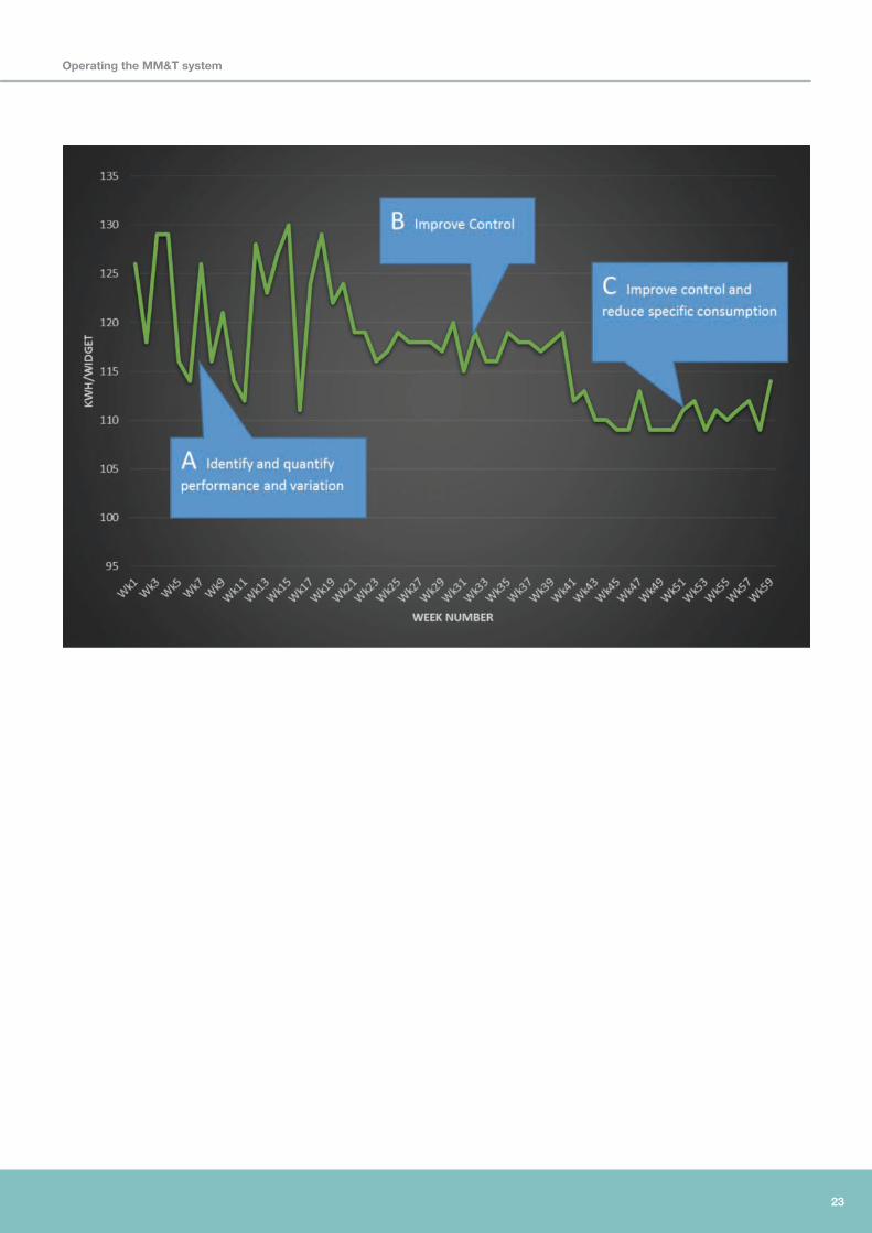
8.2 How is MM&T used to improve control and reduce energy consumption?The objective of MM&T is to understand and control some process related variable. That would usually be energy but it could equally be water consumed or waste produced or all three.

MM&T could equally be used as a quality driver and quality control indication.

It is marginally more complex than understanding the MPG of a car but the concept is similar. In this way, the MM&T system is being used to detect changes in energy performance and check on an ongoing basis that performance is being maintained. The analysis should not be complex and should allow change of performance to be detected.

In all cases the objective is to:

AFirst identify and quantify energy and cost performance

BImprove control by technology change, process optimisation or maintenance/housekeeping action

CReduce and maintain that improvement in energy efficiency

Operating the MM&T system

23

Operating the MM&T system

24

9.0 Calculating Standards9.1 Specific energy consumption vs. production . . . . . . . . . . . . . . . . . . . . . . . . . . . . . . . . . . . . . . 27

9.2 Why is volume related SEC important? . . . . . . . . . . . . . . . . . . . . . . . . . . . . . . . . . . . . . . . . . . . 28

9.3 Regression analysis . . . . . . . . . . . . . . . . . . . . . . . . . . . . . . . . . . . . . . . . . . . . . . . . . . . . . . . . . . 28

9.4 Alternative solutions for target setting. . . . . . . . . . . . . . . . . . . . . . . . . . . . . . . . . . . . . . . . . . . . 28

25

Calculating Standards

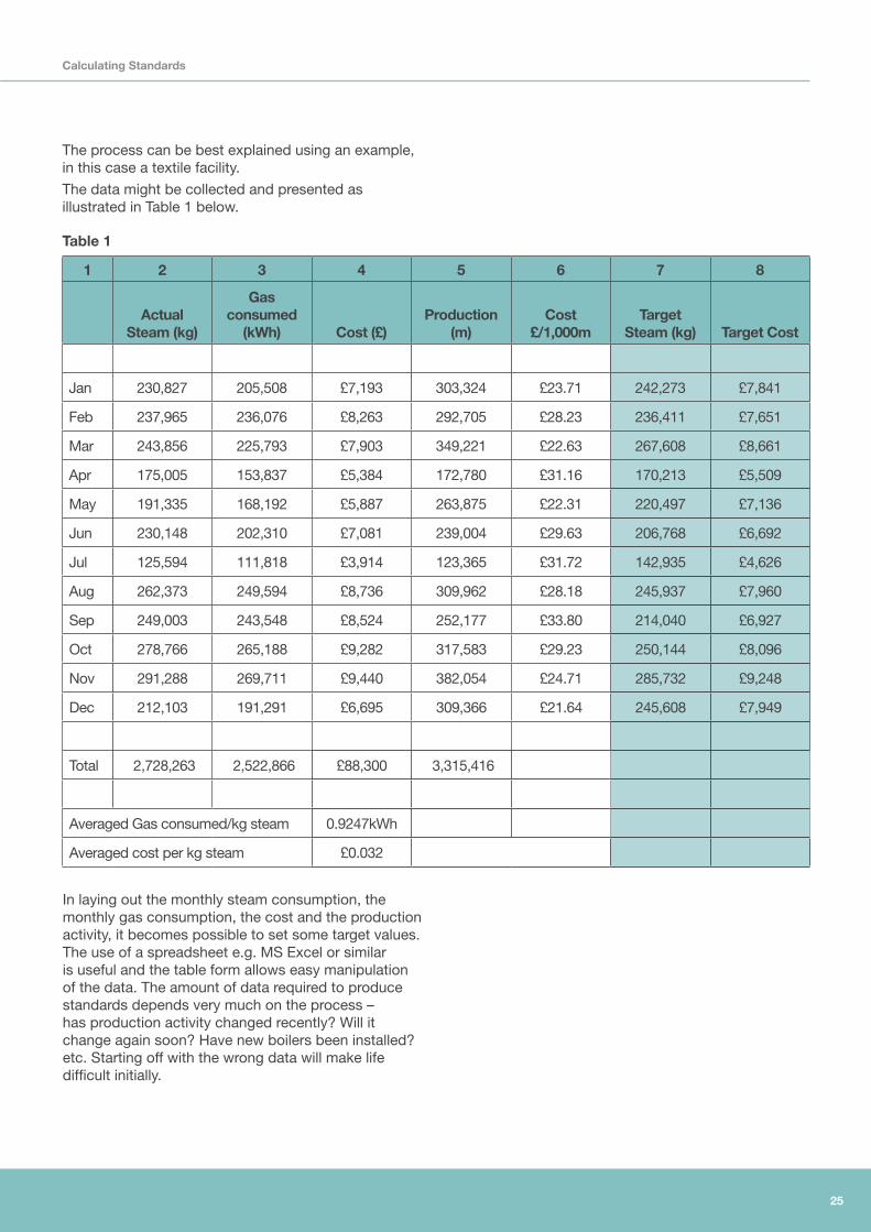
The process can be best explained using an example, in this case a textile facility.

The data might be collected and presented as illustrated in Table 1 below.

Table 1

1 2 3 4 5 6 7 8

Actual Steam (kg)

Gas consumed

(kWh) Cost (£)Production

(m)Cost

£/1,000mTarget

Steam (kg) Target Cost

Jan 230,827 205,508 £7,193 303,324 £23.71 242,273 £7,841

Feb 237,965 236,076 £8,263 292,705 £28.23 236,411 £7,651

Mar 243,856 225,793 £7,903 349,221 £22.63 267,608 £8,661

Apr 175,005 153,837 £5,384 172,780 £31.16 170,213 £5,509

May 191,335 168,192 £5,887 263,875 £22.31 220,497 £7,136

Jun 230,148 202,310 £7,081 239,004 £29.63 206,768 £6,692

Jul 125,594 111,818 £3,914 123,365 £31.72 142,935 £4,626

Aug 262,373 249,594 £8,736 309,962 £28.18 245,937 £7,960

Sep 249,003 243,548 £8,524 252,177 £33.80 214,040 £6,927

Oct 278,766 265,188 £9,282 317,583 £29.23 250,144 £8,096

Nov 291,288 269,711 £9,440 382,054 £24.71 285,732 £9,248

Dec 212,103 191,291 £6,695 309,366 £21.64 245,608 £7,949

Total 2,728,263 2,522,866 £88,300 3,315,416

Averaged Gas consumed/kg steam 0.9247kWh

Averaged cost per kg steam £0.032

In laying out the monthly steam consumption, the monthly gas consumption, the cost and the production activity, it becomes possible to set some target values. The use of a spreadsheet e.g. MS Excel or similar is useful and the table form allows easy manipulation of the data. The amount of data required to produce standards depends very much on the process – has production activity changed recently? Will it change again soon? Have new boilers been installed? etc. Starting off with the wrong data will make life difficult initially.

26

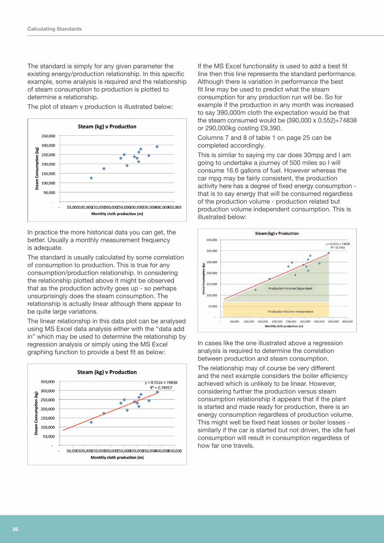
The standard is simply for any given parameter the existing energy/production relationship. In this specific example, some analysis is required and the relationship of steam consumption to production is plotted to determine a relationship.

The plot of steam v production is illustrated below:

In practice the more historical data you can get, the better. Usually a monthly measurement frequency is adequate.

The standard is usually calculated by some correlation of consumption to production. This is true for any consumption/production relationship. In considering the relationship plotted above it might be observed that as the production activity goes up - so perhaps unsurprisingly does the steam consumption. The relationship is actually linear although there appear to be quite large variations.

The linear relationship in this data plot can be analysed using MS Excel data analysis either with the “data add in” which may be used to determine the relationship by regression analysis or simply using the MS Excel graphing function to provide a best fit as below:

If the MS Excel functionality is used to add a best fit line then this line represents the standard performance. Although there is variation in performance the best fit line may be used to predict what the steam consumption for any production run will be. So for example if the production in any month was increased to say 390,000m cloth the expectation would be that the steam consumed would be (390,000 x 0.552)+74838 or 290,000kg costing £9,390.

Columns 7 and 8 of table 1 on page 25 can be completed accordingly.

This is similar to saying my car does 30mpg and I am going to undertake a journey of 500 miles so I will consume 16.6 gallons of fuel. However whereas the car mpg may be fairly consistent, the production activity here has a degree of fixed energy consumption - that is to say energy that will be consumed regardless of the production volume - production related but production volume independent consumption. This is illustrated below:

In cases like the one illustrated above a regression analysis is required to determine the correlation between production and steam consumption.

The relationship may of course be very different and the next example considers the boiler efficiency achieved which is unlikely to be linear. However, considering further the production versus steam consumption relationship it appears that if the plant is started and made ready for production, there is an energy consumption regardless of production volume. This might well be fixed heat losses or boiler losses - similarly if the car is started but not driven, the idle fuel consumption will result in consumption regardless of how far one travels.


27

Although the boiler performance might vary, this established relationship is likely to be satisfactory for ensuring that performance is maintained. Additionally this relationship may be used for the purposes of cost estimating and determining any improvements in efficiency. This technique is suitable for many simple consumption versus production relationships where the energy consumed varies as some function of production.

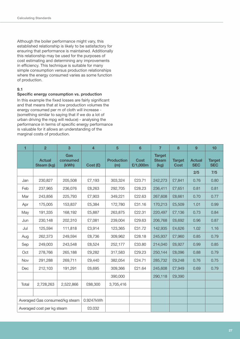
9.1 Specific energy consumption vs. productionIn this example the fixed losses are fairly significant and that means that at low production volumes the energy consumed per m of cloth will increase - (something similar to saying that if we do a lot of urban driving the mpg will reduce) - analysing the performance in terms of specific energy performance is valuable for it allows an understanding of the marginal costs of production.

1 2 3 4 5 6 7 8 9 10

Actual Steam (kg)

Gas consumed

(kWh) Cost (£)Production

(m)Cost

£/1,000m

Target Steam

(kg) Target Cost

Actual SEC

Target SEC

2/5 7/5

Jan 230,827 205,508 £7,193 303,324 £23.71 242,273 £7,841 0.76 0.80

Feb 237,965 236,076 £8,263 292,705 £28.23 236,411 £7,651 0.81 0.81

Mar 243,856 225,793 £7,903 349,221 £22.63 267,608 £8,661 0.70 0.77

Apr 175,005 153,837 £5,384 172,780 £31.16 170,213 £5,509 1.01 0.99

May 191,335 168,192 £5,887 263,875 £22.31 220,497 £7,136 0.73 0.84

Jun 230,148 202,310 £7,081 239,004 £29.63 206,768 £6,692 0.96 0.87

Jul 125,594 111,818 £3,914 123,365 £31.72 142,935 £4,626 1.02 1.16

Aug 262,373 249,594 £8,736 309,962 £28.18 245,937 £7,960 0.85 0.79

Sep 249,003 243,548 £8,524 252,177 £33.80 214,040 £6,927 0.99 0.85

Oct 278,766 265,188 £9,282 317,583 £29.23 250,144 £8,096 0.88 0.79

Nov 291,288 269,711 £9,440 382,054 £24.71 285,732 £9,248 0.76 0.75

Dec 212,103 191,291 £6,695 309,366 £21.64 245,608 £7,949 0.69 0.79

390,000 290,118 £9,390

Total 2,728,263 2,522,866 £88,300 3,705,416

Averaged Gas consumed/kg steam 0.9247kWh

Averaged cost per kg steam £0.032


28

If the specific energy consumption indicator is calculated for each of the standard data entries - then a SEC can be calculated.

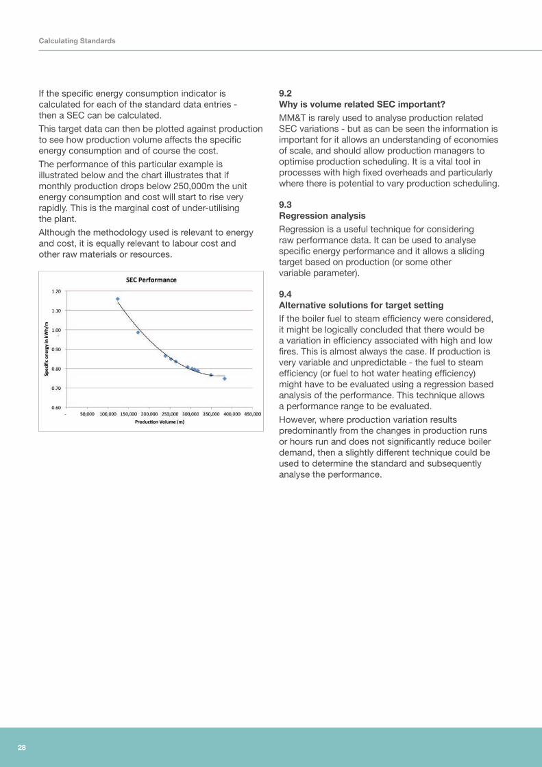
This target data can then be plotted against production to see how production volume affects the specific energy consumption and of course the cost.

The performance of this particular example is illustrated below and the chart illustrates that if monthly production drops below 250,000m the unit energy consumption and cost will start to rise very rapidly. This is the marginal cost of under-utilising the plant.

Although the methodology used is relevant to energy and cost, it is equally relevant to labour cost and other raw materials or resources.

9.2 Why is volume related SEC important?MM&T is rarely used to analyse production related SEC variations - but as can be seen the information is important for it allows an understanding of economies of scale, and should allow production managers to optimise production scheduling. It is a vital tool in processes with high fixed overheads and particularly where there is potential to vary production scheduling.

9.3 Regression analysisRegression is a useful technique for considering raw performance data. It can be used to analyse specific energy performance and it allows a sliding target based on production (or some other variable parameter).

9.4 Alternative solutions for target setting If the boiler fuel to steam efficiency were considered, it might be logically concluded that there would be a variation in efficiency associated with high and low fires. This is almost always the case. If production is very variable and unpredictable - the fuel to steam efficiency (or fuel to hot water heating efficiency) might have to be evaluated using a regression based analysis of the performance. This technique allows a performance range to be evaluated.

However, where production variation results predominantly from the changes in production runs or hours run and does not significantly reduce boiler demand, then a slightly different technique could be used to determine the standard and subsequently analyse the performance.


29

If the data for a boiler operation is considered:-

Gas Consumed (kWh) Steam Produced (kg) Energy is steam (kWh) Fuel to steam ratio Week 1 54,700 67,037 43,760 80.0

Week 2 45,401 52,163 34,051 75.0

Week 3 48,683 55,934 36,512 75.0

Week 4 53,606 63,232 41,277 77.0

Week 5 47,042 57,651 37,634 80.0

Week 6 53,059 61,774 40,325 76.0

Week 7 44,307 50,227 32,787 74.0

Week 8 48,683 58,171 37,973 78.0

Week 9 45,401 50,772 33,143 73.0

Week 10 43,760 54,300 35,446 81.0

Week 11 53,606 65,696 42,885 80.0

Week 12 47,589 54,677 35,692 75.0

Week 13 47,589 54,677 35,692 75.0

Week 14 53,059 63,400 41,386 78.0

Week 15 53,606 62,411 40,741 76.0

Week 16 44,307 49,548 32,344 73.0

Week 17 49,777 61,003 39,822 80.0

Week 18 45,401 50,772 33,143 73.0

Week 19 43,760 54,970 35,883 82.0

Week 20 53,606 64,875 42,349 79.0

Week 21 49,230 55,808 36,430 74.0

Week 22 50,324 57,048 37,240 74.0

Week 23 49,230 56,562 36,923 75.0

Week 24 50,324 58,590 38,246 76.0

Week 25 48,683 59,663 38,946 80.0

Week 26 54,700 61,171 39,931 73.0

Week 27 51,965 61,297 40,013 77.0

Week 28 53,606 59,947 39,132 73.0

Week 29 49,230 60,333 39,384 80.0

Week 30 54,153 67,196 43,864 81.0

Week 31 43,760 50,948 33,258 76.0

Week 32 51,418 59,864 39,078 76.0

Week 33 44,307 51,585 33,673 76.0

Week 34 54,153 68,025 44,405 82.0

Week 35 50,324 57,048 37,240 74.0

Week 36 51,418 59,864 39,078 76.0

Week 37 44,854 54,283 35,435 79.0

Week 38 51,418 61,439 40,106 78.0

Week 39 49,230 61,087 39,876 81.0

Week 40 45,401 52,163 34,051 75.0

Week 41 45,401 57,031 37,229 82.0

Week 42 50,324 61,674 40,259 80.0

Week 43 47,042 53,328 34,811 74.0

Week 44 44,307 49,548 32,344 73.0

Week 45 45,948 54,199 35,380 77.0

Week 46 53,606 64,053 41,813 78.0

Week 47 54,700 64,523 42,119 77.0

Week 48 49,777 57,191 37,333 75.0

Week 49 50,871 63,123 41,206 81.0

Week 50 50,871 59,227 38,662 76.0

Week 51 54,700 65,361 42,666 78.0


30

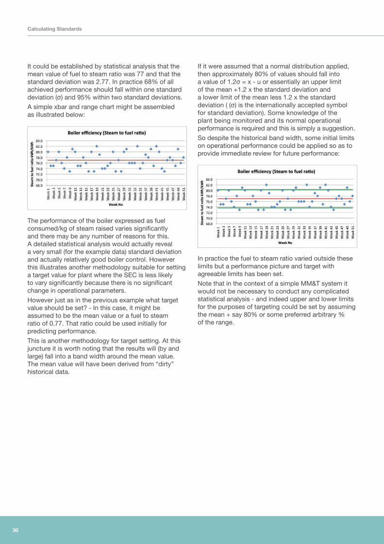
It could be established by statistical analysis that the mean value of fuel to steam ratio was 77 and that the standard deviation was 2.77. In practice 68% of all achieved performance should fall within one standard deviation (σ) and 95% within two standard deviations.

A simple xbar and range chart might be assembled as illustrated below:

The performance of the boiler expressed as fuel consumed/kg of steam raised varies significantly and there may be any number of reasons for this. A detailed statistical analysis would actually reveal a very small (for the example data) standard deviation and actually relatively good boiler control. However this illustrates another methodology suitable for setting a target value for plant where the SEC is less likely to vary significantly because there is no significant change in operational parameters.

However just as in the previous example what target value should be set? - In this case, it might be assumed to be the mean value or a fuel to steam ratio of 0.77. That ratio could be used initially for predicting performance.

This is another methodology for target setting. At this juncture it is worth noting that the results will (by and large) fall into a band width around the mean value. The mean value will have been derived from “dirty” historical data.

If it were assumed that a normal distribution applied, then approximately 80% of values should fall into a value of 1.2σ = x - u or essentially an upper limit of the mean +1.2 x the standard deviation and a lower limit of the mean less 1.2 x the standard deviation ( (σ) is the internationally accepted symbol for standard deviation). Some knowledge of the plant being monitored and its normal operational performance is required and this is simply a suggestion.

So despite the historical band width, some initial limits on operational performance could be applied so as to provide immediate review for future performance:

In practice the fuel to steam ratio varied outside these limits but a performance picture and target with agreeable limits has been set.

Note that in the context of a simple MM&T system it would not be necessary to conduct any complicated statistical analysis - and indeed upper and lower limits for the purposes of targeting could be set by assuming the mean + say 80% or some preferred arbitrary % of the range.


31

10.1 Identifying trends . . . . . . . . . . . . . . . . . . . . . . . . . . . . . . . . . . . . . . . . . . . . . . . . . . . . . . . 32

10.2 Improving consistency and accuracy . . . . . . . . . . . . . . . . . . . . . . . . . . . . . . . . . . . . . . . 32

10.0 Evaluating performance change

Evaluating performance change

32

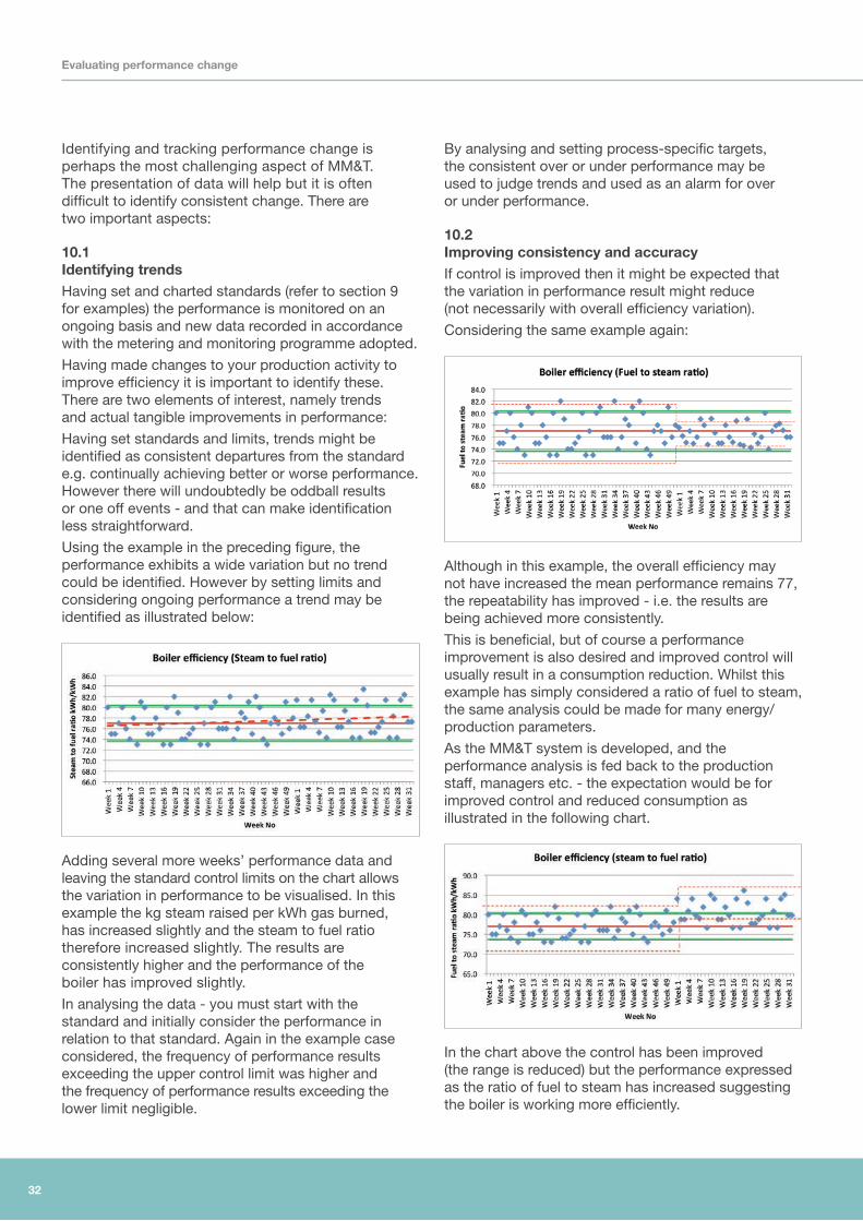
Identifying and tracking performance change is perhaps the most challenging aspect of MM&T. The presentation of data will help but it is often difficult to identify consistent change. There are two important aspects:

10.1 Identifying trendsHaving set and charted standards (refer to section 9 for examples) the performance is monitored on an ongoing basis and new data recorded in accordance with the metering and monitoring programme adopted.

Having made changes to your production activity to improve efficiency it is important to identify these. There are two elements of interest, namely trends and actual tangible improvements in performance:

Having set standards and limits, trends might be identified as consistent departures from the standard e.g. continually achieving better or worse performance. However there will undoubtedly be oddball results or one off events - and that can make identification less straightforward.

Using the example in the preceding figure, the performance exhibits a wide variation but no trend could be identified. However by setting limits and considering ongoing performance a trend may be identified as illustrated below:

Adding several more weeks’ performance data and leaving the standard control limits on the chart allows the variation in performance to be visualised. In this example the kg steam raised per kWh gas burned, has increased slightly and the steam to fuel ratio therefore increased slightly. The results are consistently higher and the performance of the boiler has improved slightly.

In analysing the data - you must start with the standard and initially consider the performance in relation to that standard. Again in the example case considered, the frequency of performance results exceeding the upper control limit was higher and the frequency of performance results exceeding the lower limit negligible.

By analysing and setting process-specific targets, the consistent over or under performance may be used to judge trends and used as an alarm for over or under performance.

10.2 Improving consistency and accuracyIf control is improved then it might be expected that the variation in performance result might reduce (not necessarily with overall efficiency variation).

Considering the same example again:

Although in this example, the overall efficiency may not have increased the mean performance remains 77, the repeatability has improved - i.e. the results are being achieved more consistently.

This is beneficial, but of course a performance improvement is also desired and improved control will usually result in a consumption reduction. Whilst this example has simply considered a ratio of fuel to steam, the same analysis could be made for many energy/production parameters.

As the MM&T system is developed, and the performance analysis is fed back to the production staff, managers etc. - the expectation would be for improved control and reduced consumption as illustrated in the following chart.

In the chart above the control has been improved (the range is reduced) but the performance expressed as the ratio of fuel to steam has increased suggesting the boiler is working more efficiently.

33

Evaluating performance change

In practice it is sometimes difficult to detect these changes and a CUSUM (cumulative sum of errors) technique may be used to identify and track improvements. (CUSUM is addressed in the next guide section).

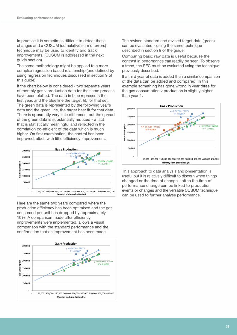
The same methodology might be applied to a more complex regression based relationship (one defined by using regression techniques discussed in section 9 of this guide).

If the chart below is considered - two separate years of monthly gas v production data for the same process have been plotted. The data in blue represents the first year, and the blue line the target fit, for that set. The green data is represented by the following year’s data and the green line, the target best fit for that data. There is apparently very little difference, but the spread of the green data is substantially reduced - a fact that is statistically meaningful and reflected in the correlation co-efficient of the data which is much higher. On first examination, the control has been improved, albeit with little efficiency improvement.

Here are the same two years compared where the production efficiency has been optimised and the gas consumed per unit has dropped by approximately 10%. A comparison made after efficiency improvements were implemented, allows a visual comparison with the standard performance and the confirmation that an improvement has been made.

The revised standard and revised target data (green) can be evaluated - using the same technique described in section 9 of the guide.

Comparing basic raw data is useful because the contrast in performance can readily be seen. To observe a trend, the SEC must be evaluated using the technique previously described.

If a third year of data is added then a similar comparison of the data can be added and compared. In this example something has gone wrong in year three for the gas consumption v production is slightly higher than year 1.

This approach to data analysis and presentation is useful but it is relatively difficult to discern when things changed or the time of change - often the time of performance change can be linked to production events or changes and the versatile CUSUM technique can be used to further analyse performance.

34

11.1 CUSUM convention . . . . . . . . . . . . . . . . . . . . . . . . . . . . . . . . . . . . . . . . . . . . . . . . . . . . . 38

11.2 Caution with CUSUM . . . . . . . . . . . . . . . . . . . . . . . . . . . . . . . . . . . . . . . . . . . . . . . . . . . . 38

11.0 CUSUM Techniques (Cumulative sum of errors)

35

Interpreting changes in data can be awkward, particularly where there is a large data set and or there are unlogged production changes. The CUSUM analysis is helpful in understanding when performance changed and whether it is being maintained.

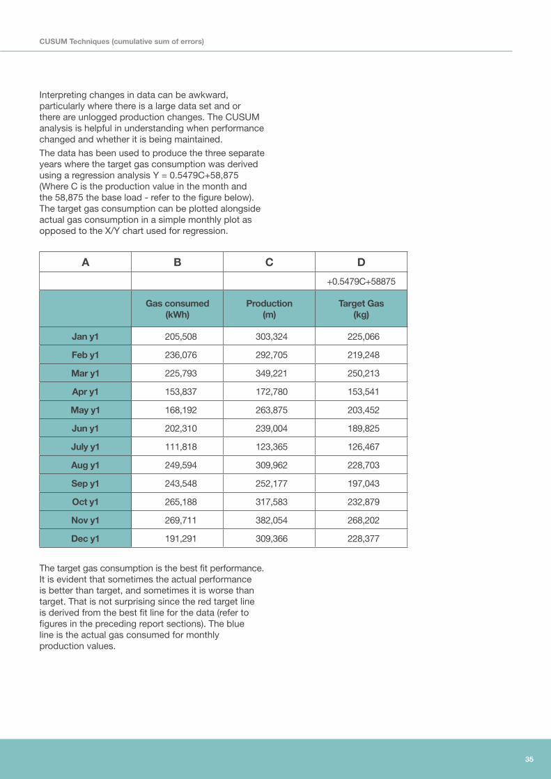
The data has been used to produce the three separate years where the target gas consumption was derived using a regression analysis Y = 0.5479C+58,875 (Where C is the production value in the month and the 58,875 the base load - refer to the figure below). The target gas consumption can be plotted alongside actual gas consumption in a simple monthly plot as opposed to the X/Y chart used for regression.

A B C D

+0.5479C+58875

Gas consumed (kWh)

Production (m)

Target Gas (kg)

Jan y1 205,508 303,324 225,066

Feb y1 236,076 292,705 219,248

Mar y1 225,793 349,221 250,213

Apr y1 153,837 172,780 153,541

May y1 168,192 263,875 203,452

Jun y1 202,310 239,004 189,825

July y1 111,818 123,365 126,467

Aug y1 249,594 309,962 228,703

Sep y1 243,548 252,177 197,043

Oct y1 265,188 317,583 232,879

Nov y1 269,711 382,054 268,202

Dec y1 191,291 309,366 228,377

The target gas consumption is the best fit performance. It is evident that sometimes the actual performance is better than target, and sometimes it is worse than target. That is not surprising since the red target line is derived from the best fit line for the data (refer to figures in the preceding report sections). The blue line is the actual gas consumed for monthly production values.

CUSUM Techniques (cumulative sum of errors)

36


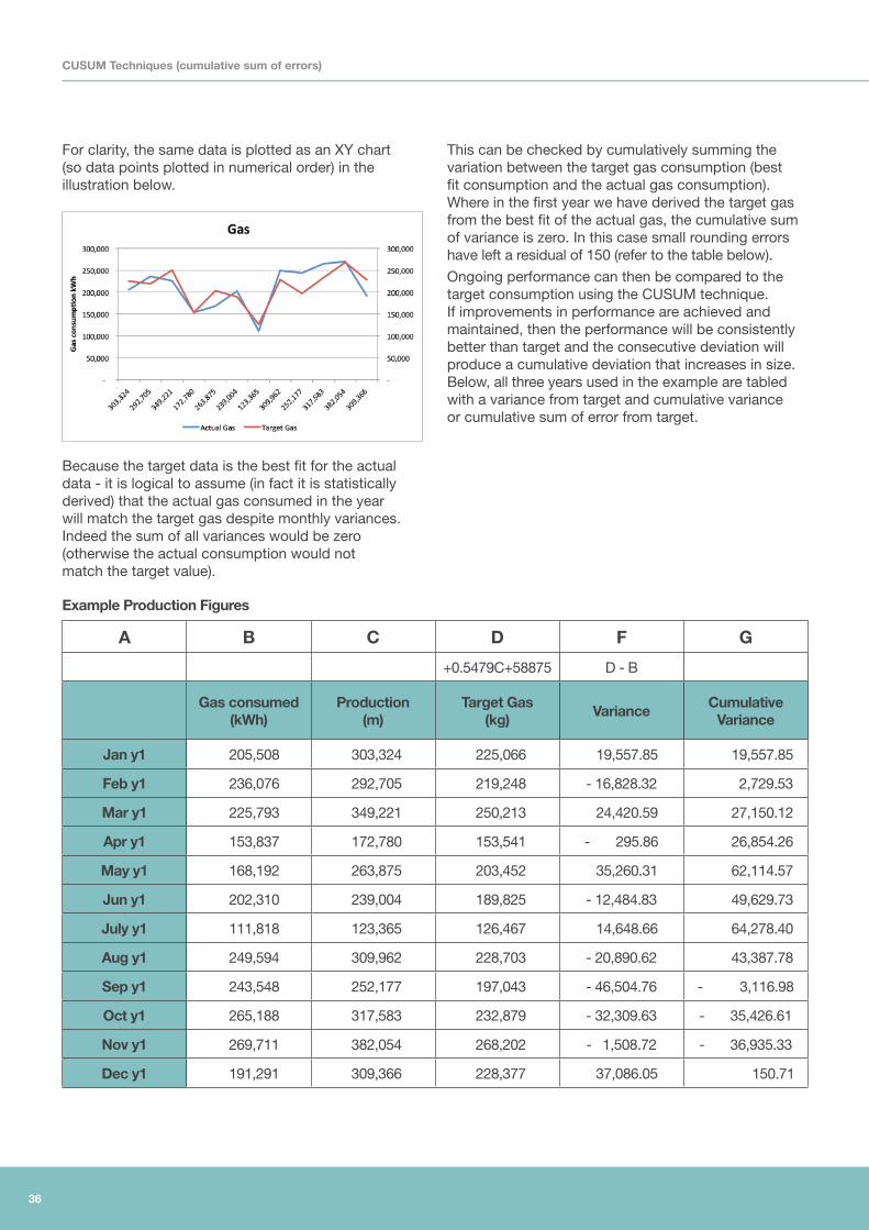
For clarity, the same data is plotted as an XY chart (so data points plotted in numerical order) in the illustration below.

Because the target data is the best fit for the actual data - it is logical to assume (in fact it is statistically derived) that the actual gas consumed in the year will match the target gas despite monthly variances. Indeed the sum of all variances would be zero (otherwise the actual consumption would not match the target value).

Example Production Figures

A B C D F G

+0.5479C+58875 D - B

Gas consumed (kWh)

Production (m)

Target Gas (kg)

VarianceCumulative

Variance

Jan y1 205,508 303,324 225,066 19,557.85 19,557.85

Feb y1 236,076 292,705 219,248 - 16,828.32 2,729.53

Mar y1 225,793 349,221 250,213 24,420.59 27,150.12

Apr y1 153,837 172,780 153,541 - 295.86 26,854.26

May y1 168,192 263,875 203,452 35,260.31 62,114.57

Jun y1 202,310 239,004 189,825 - 12,484.83 49,629.73

July y1 111,818 123,365 126,467 14,648.66 64,278.40

Aug y1 249,594 309,962 228,703 - 20,890.62 43,387.78

Sep y1 243,548 252,177 197,043 - 46,504.76 - 3,116.98

Oct y1 265,188 317,583 232,879 - 32,309.63 - 35,426.61

Nov y1 269,711 382,054 268,202 - 1,508.72 - 36,935.33

Dec y1 191,291 309,366 228,377 37,086.05 150.71

This can be checked by cumulatively summing the variation between the target gas consumption (best fit consumption and the actual gas consumption). Where in the first year we have derived the target gas from the best fit of the actual gas, the cumulative sum of variance is zero. In this case small rounding errors have left a residual of 150 (refer to the table below).

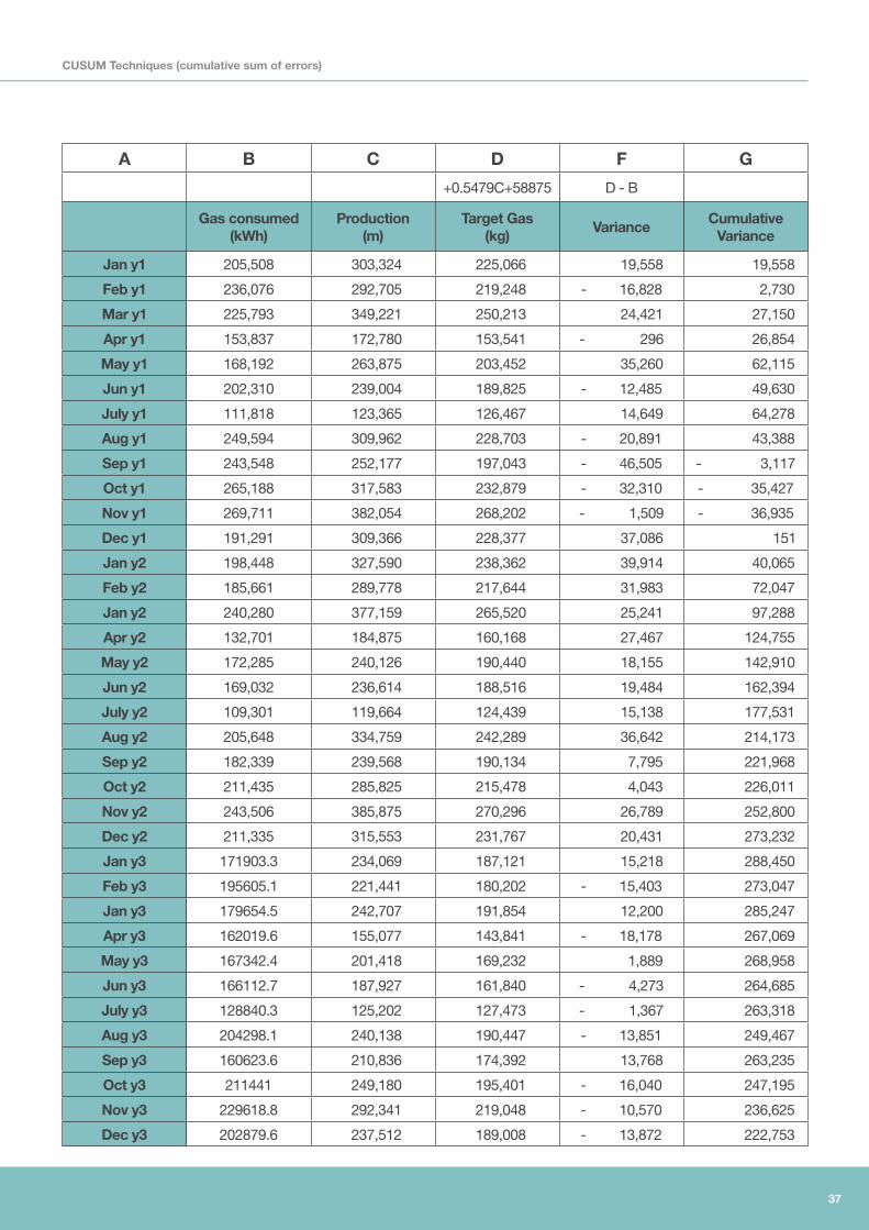
Ongoing performance can then be compared to the target consumption using the CUSUM technique. If improvements in performance are achieved and maintained, then the performance will be consistently better than target and the consecutive deviation will produce a cumulative deviation that increases in size. Below, all three years used in the example are tabled with a variance from target and cumulative variance or cumulative sum of error from target.

37

A B C D F G

+0.5479C+58875 D - B

Gas consumed (kWh)

Production (m)

Target Gas (kg)

VarianceCumulative

Variance

Jan y1 205,508 303,324 225,066 19,558 19,558

Feb y1 236,076 292,705 219,248 - 16,828 2,730

Mar y1 225,793 349,221 250,213 24,421 27,150

Apr y1 153,837 172,780 153,541 - 296 26,854

May y1 168,192 263,875 203,452 35,260 62,115

Jun y1 202,310 239,004 189,825 - 12,485 49,630

July y1 111,818 123,365 126,467 14,649 64,278

Aug y1 249,594 309,962 228,703 - 20,891 43,388

Sep y1 243,548 252,177 197,043 - 46,505 - 3,117

Oct y1 265,188 317,583 232,879 - 32,310 - 35,427

Nov y1 269,711 382,054 268,202 - 1,509 - 36,935

Dec y1 191,291 309,366 228,377 37,086 151

Jan y2 198,448 327,590 238,362 39,914 40,065

Feb y2 185,661 289,778 217,644 31,983 72,047

Jan y2 240,280 377,159 265,520 25,241 97,288

Apr y2 132,701 184,875 160,168 27,467 124,755

May y2 172,285 240,126 190,440 18,155 142,910

Jun y2 169,032 236,614 188,516 19,484 162,394

July y2 109,301 119,664 124,439 15,138 177,531

Aug y2 205,648 334,759 242,289 36,642 214,173

Sep y2 182,339 239,568 190,134 7,795 221,968

Oct y2 211,435 285,825 215,478 4,043 226,011

Nov y2 243,506 385,875 270,296 26,789 252,800

Dec y2 211,335 315,553 231,767 20,431 273,232

Jan y3 171903.3 234,069 187,121 15,218 288,450

Feb y3 195605.1 221,441 180,202 - 15,403 273,047

Jan y3 179654.5 242,707 191,854 12,200 285,247

Apr y3 162019.6 155,077 143,841 - 18,178 267,069

May y3 167342.4 201,418 169,232 1,889 268,958

Jun y3 166112.7 187,927 161,840 - 4,273 264,685

July y3 128840.3 125,202 127,473 - 1,367 263,318

Aug y3 204298.1 240,138 190,447 - 13,851 249,467

Sep y3 160623.6 210,836 174,392 13,768 263,235

Oct y3 211441 249,180 195,401 - 16,040 247,195

Nov y3 229618.8 292,341 219,048 - 10,570 236,625

Dec y3 202879.6 237,512 189,008 - 13,872 222,753


38

Now since the variance has been defined as the difference between the target and the actual consumption, it follows that if the plant performance is consistently improved, there will be a constant positive variance. With a consistent positive variance from the time of improvement, the cumulative error will grow consistently compounding the error month on month.

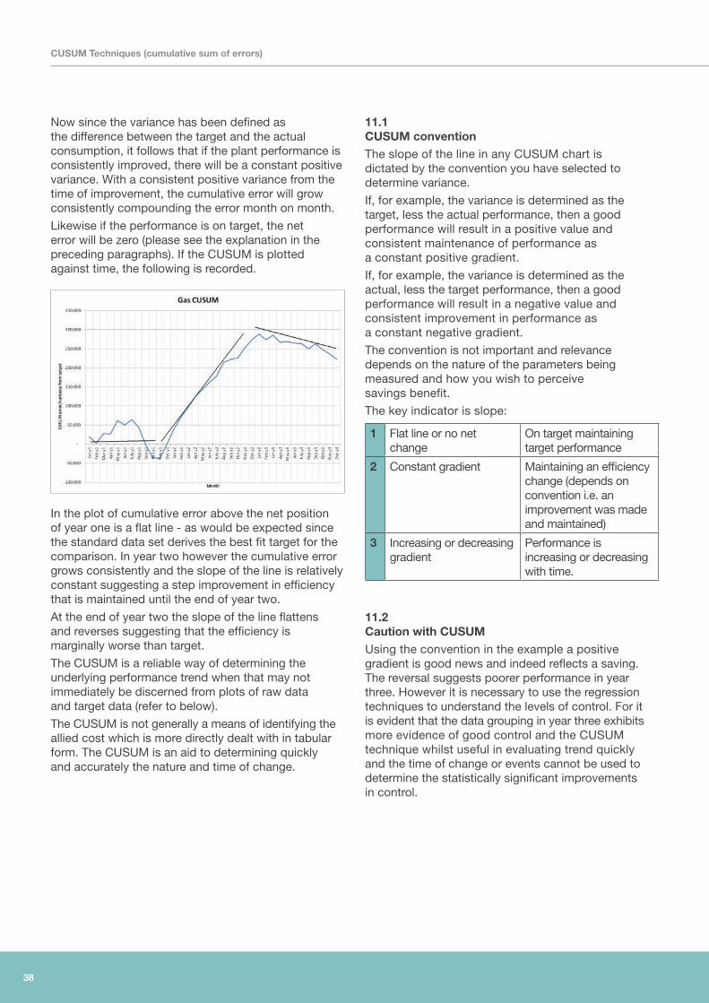
Likewise if the performance is on target, the net error will be zero (please see the explanation in the preceding paragraphs). If the CUSUM is plotted against time, the following is recorded.

In the plot of cumulative error above the net position of year one is a flat line - as would be expected since the standard data set derives the best fit target for the comparison. In year two however the cumulative error grows consistently and the slope of the line is relatively constant suggesting a step improvement in efficiency that is maintained until the end of year two.

At the end of year two the slope of the line flattens and reverses suggesting that the efficiency is marginally worse than target.

The CUSUM is a reliable way of determining the underlying performance trend when that may not immediately be discerned from plots of raw data and target data (refer to below).

The CUSUM is not generally a means of identifying the allied cost which is more directly dealt with in tabular form. The CUSUM is an aid to determining quickly and accurately the nature and time of change.

11.1 CUSUM conventionThe slope of the line in any CUSUM chart is dictated by the convention you have selected to determine variance.

If, for example, the variance is determined as the target, less the actual performance, then a good performance will result in a positive value and consistent maintenance of performance as a constant positive gradient.

If, for example, the variance is determined as the actual, less the target performance, then a good performance will result in a negative value and consistent improvement in performance as a constant negative gradient.

The convention is not important and relevance depends on the nature of the parameters being measured and how you wish to perceive savings benefit.

The key indicator is slope:

1 Flat line or no net change

On target maintaining target performance

2 Constant gradient Maintaining an efficiency change (depends on convention i.e. an improvement was made and maintained)

3 Increasing or decreasing gradient

Performance is increasing or decreasing with time.

11.2 Caution with CUSUMUsing the convention in the example a positive gradient is good news and indeed reflects a saving. The reversal suggests poorer performance in year three. However it is necessary to use the regression techniques to understand the levels of control. For it is evident that the data grouping in year three exhibits more evidence of good control and the CUSUM technique whilst useful in evaluating trend quickly and the time of change or events cannot be used to determine the statistically significant improvements in control.


39

12.0 Feedback and reporting

40

Feedback and reporting

In most cases the benefit of simply comparing energy consumption with a calendar period is inadequate. Generally a production adjusted comparison must be made. The techniques explained and exampled in this guide allow you to do that.

Reporting and acting on the reports (which requires the engagement of the production staff) is the vital element of MM&T. MM&T is as much about understanding production and quality control as it is about managing energy.

People understand data in different ways, however generally graphical information is more readily and quickly understood. For each cost centre eventually selected there must be a simple report that shows and explains:

• What is the target performance for the cost centre?

• How does current performance compare with the target?

• Is the performance-getting better or worse?

• What is the extent of under or over achievement?

• What is the projected cost implication of the performance?

• Trend information.

A report for each cost centre might typically therefore contain a comparison for each measured SEC with a regression based target. It might provide an assessment of the cost of being above or below target and what is the best performance thus far.

The report would generally also provide a cumulative Year to Date (YTD) total of above and below target.

The regression chart might show the performance month on month plotted against the historical target. The fictitious charts used in the preceding illustrations, suggests regular “better than target” performance. However, that can be confirmed easily using both the control chart and the CUSUM chart to examine the degree of performance variation from an historical mean. Target limits set as described in this report and the cumulative performance improvement (or impairment) may also be used.

The fictitious CUSUM chart indicates the maintenance (steady positive gradient) of a 3% improvement illustrating the cumulative energy saving (remember this is convention specific).

All of the above may be completely automated in a customised spreadsheet or bespoke MM&T software. It is relatively easy to write an Excel import macro and use the automatic data fill capabilities of Excel to produce largely automated reporting and auto ranging graphics (e.g. regardless of the table fill the graph will automatically expand and recalculate the revised targets if desired).

However as explained, the same functions can be achieved without the effort using bespoke software.

41

13.1 Degree days . . . . . . . . . . . . . . . . . . . . . . . . . . . . . . . . . . . . . . . . . . . . . . . . . . . . . . . . . . . 42

13.2 Where do I get degree day figures from? . . . . . . . . . . . . . . . . . . . . . . . . . . . . . . . . . . . . . 42

13.3 Degree Days work in practice? . . . . . . . . . . . . . . . . . . . . . . . . . . . . . . . . . . . . . . . . . . . . 45

13.4 Using the CUSUM analysis to verify trends . . . . . . . . . . . . . . . . . . . . . . . . . . . . . . . . . . . 46

13.0 How do you assess building energy performance?

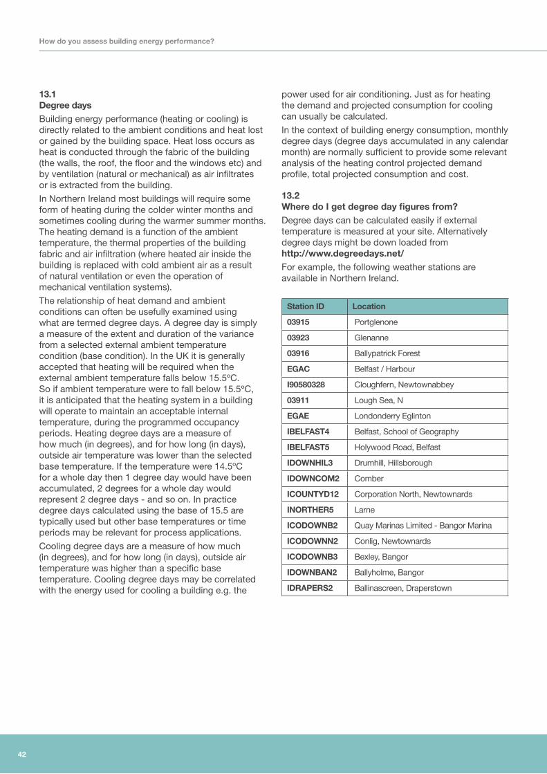
How do you assess building energy performance?

42

13.1 Degree daysBuilding energy performance (heating or cooling) is directly related to the ambient conditions and heat lost or gained by the building space. Heat loss occurs as heat is conducted through the fabric of the building (the walls, the roof, the floor and the windows etc) and by ventilation (natural or mechanical) as air infiltrates or is extracted from the building.

In Northern Ireland most buildings will require some form of heating during the colder winter months and sometimes cooling during the warmer summer months. The heating demand is a function of the ambient temperature, the thermal properties of the building fabric and air infiltration (where heated air inside the building is replaced with cold ambient air as a result of natural ventilation or even the operation of mechanical ventilation systems).

The relationship of heat demand and ambient conditions can often be usefully examined using what are termed degree days. A degree day is simply a measure of the extent and duration of the variance from a selected external ambient temperature condition (base condition). In the UK it is generally accepted that heating will be required when the external ambient temperature falls below 15.5ºC. So if ambient temperature were to fall below 15.5ºC, it is anticipated that the heating system in a building will operate to maintain an acceptable internal temperature, during the programmed occupancy periods. Heating degree days are a measure of how much (in degrees), and for how long (in days), outside air temperature was lower than the selected base temperature. If the temperature were 14.5ºC for a whole day then 1 degree day would have been accumulated, 2 degrees for a whole day would represent 2 degree days - and so on. In practice degree days calculated using the base of 15.5 are typically used but other base temperatures or time periods may be relevant for process applications.

Cooling degree days are a measure of how much (in degrees), and for how long (in days), outside air temperature was higher than a specific base temperature. Cooling degree days may be correlated with the energy used for cooling a building e.g. the

power used for air conditioning. Just as for heating the demand and projected consumption for cooling can usually be calculated.

In the context of building energy consumption, monthly degree days (degree days accumulated in any calendar month) are normally sufficient to provide some relevant analysis of the heating control projected demand profile, total projected consumption and cost.

13.2 Where do I get degree day figures from?Degree days can be calculated easily if external temperature is measured at your site. Alternatively degree days might be down loaded from http://www.degreedays.net/For example, the following weather stations are available in Northern Ireland.

Station ID Location

03915 Portglenone

03923 Glenanne

03916 Ballypatrick Forest

EGAC Belfast / Harbour

I90580328 Cloughfern, Newtownabbey

03911 Lough Sea, N

EGAE Londonderry Eglinton

IBELFAST4 Belfast, School of Geography

IBELFAST5 Holywood Road, Belfast

IDOWNHIL3 Drumhill, Hillsborough

IDOWNCOM2 Comber

ICOUNTYD12 Corporation North, Newtownards

INORTHER5 Larne

ICODOWNB2 Quay Marinas Limited - Bangor Marina

ICODOWNN2 Conlig, Newtownards

ICODOWNB3 Bexley, Bangor

IDOWNBAN2 Ballyholme, Bangor

IDRAPERS2 Ballinascreen, Draperstown

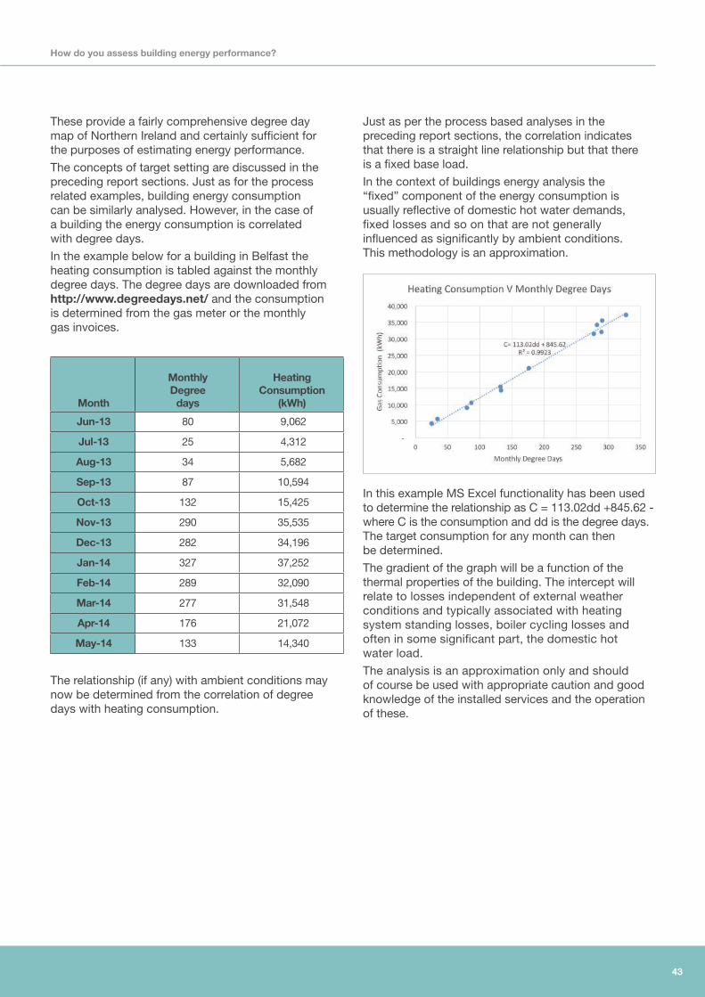
43


These provide a fairly comprehensive degree day map of Northern Ireland and certainly sufficient for the purposes of estimating energy performance.

The concepts of target setting are discussed in the preceding report sections. Just as for the process related examples, building energy consumption can be similarly analysed. However, in the case of a building the energy consumption is correlated with degree days.

In the example below for a building in Belfast the heating consumption is tabled against the monthly degree days. The degree days are downloaded from http://www.degreedays.net/ and the consumption is determined from the gas meter or the monthly gas invoices.

Month

Monthly Degree

days

Heating Consumption

(kWh)

Jun-13 80 9,062

Jul-13 25 4,312

Aug-13 34 5,682

Sep-13 87 10,594

Oct-13 132 15,425

Nov-13 290 35,535

Dec-13 282 34,196

Jan-14 327 37,252

Feb-14 289 32,090

Mar-14 277 31,548

Apr-14 176 21,072

May-14 133 14,340

The relationship (if any) with ambient conditions may now be determined from the correlation of degree days with heating consumption.

Just as per the process based analyses in the preceding report sections, the correlation indicates that there is a straight line relationship but that there is a fixed base load.

In the context of buildings energy analysis the “fixed” component of the energy consumption is usually reflective of domestic hot water demands, fixed losses and so on that are not generally influenced as significantly by ambient conditions. This methodology is an approximation.

In this example MS Excel functionality has been used to determine the relationship as C = 113.02dd +845.62 - where C is the consumption and dd is the degree days. The target consumption for any month can then be determined.

The gradient of the graph will be a function of the thermal properties of the building. The intercept will relate to losses independent of external weather conditions and typically associated with heating system standing losses, boiler cycling losses and often in some significant part, the domestic hot water load.

The analysis is an approximation only and should of course be used with appropriate caution and good knowledge of the installed services and the operation of these.

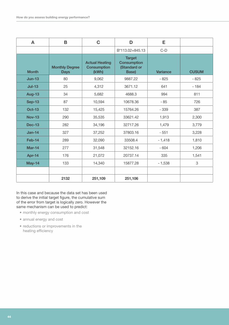
44

In this case and because the data set has been used to derive the initial target figure, the cumulative sum of the error from target is logically zero. However the same mechanism can be used to predict:

• monthly energy consumption and cost

• annual energy and cost

• reductions or improvements in the heating efficiency

A B C D E

B*113.02+845.13 C-D

MonthMonthly Degree

Days

Actual Heating Consumption

(kWh)

Target Consumption (Standard or

Base) Variance CUSUM

Jun-13 80 9,062 9887.22 - 825 - 825

Jul-13 25 4,312 3671.12 641 - 184

Aug-13 34 5,682 4688.3 994 811

Sep-13 87 10,594 10678.36 - 85 726

Oct-13 132 15,425 15764.26 - 339 387

Nov-13 290 35,535 33621.42 1,913 2,300

Dec-13 282 34,196 32717.26 1,479 3,779

Jan-14 327 37,252 37803.16 - 551 3,228

Feb-14 289 32,090 33508.4 - 1,418 1,810

Mar-14 277 31,548 32152.16 - 604 1,206

Apr-14 176 21,072 20737.14 335 1,541

May-14 133 14,340 15877.28 - 1,538 3

2132 251,109 251,106


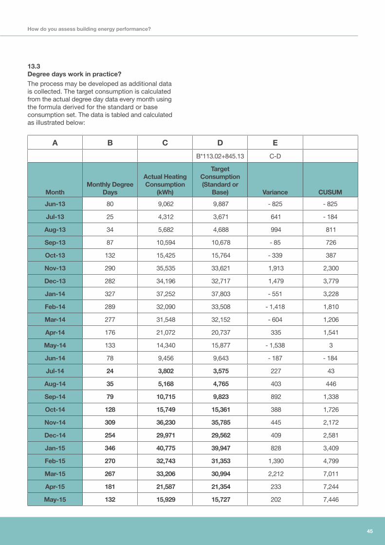
45

13.3 Degree days work in practice?The process may be developed as additional data is collected. The target consumption is calculated from the actual degree day data every month using the formula derived for the standard or base consumption set. The data is tabled and calculated as illustrated below:

A B C D E

B*113.02+845.13 C-D

MonthMonthly Degree

Days

Actual Heating Consumption

(kWh)

Target Consumption (Standard or

Base) Variance CUSUM

Jun-13 80 9,062 9,887 - 825 - 825

Jul-13 25 4,312 3,671 641 - 184

Aug-13 34 5,682 4,688 994 811

Sep-13 87 10,594 10,678 - 85 726

Oct-13 132 15,425 15,764 - 339 387

Nov-13 290 35,535 33,621 1,913 2,300

Dec-13 282 34,196 32,717 1,479 3,779

Jan-14 327 37,252 37,803 - 551 3,228

Feb-14 289 32,090 33,508 - 1,418 1,810

Mar-14 277 31,548 32,152 - 604 1,206

Apr-14 176 21,072 20,737 335 1,541

May-14 133 14,340 15,877 - 1,538 3

Jun-14 78 9,456 9,643 - 187 - 184

Jul-14 24 3,802 3,575 227 43

Aug-14 35 5,168 4,765 403 446

Sep-14 79 10,715 9,823 892 1,338

Oct-14 128 15,749 15,361 388 1,726

Nov-14 309 36,230 35,785 445 2,172

Dec-14 254 29,971 29,562 409 2,581

Jan-15 346 40,775 39,947 828 3,409

Feb-15 270 32,743 31,353 1,390 4,799

Mar-15 267 33,206 30,994 2,212 7,011

Apr-15 181 21,587 21,354 233 7,244

May-15 132 15,929 15,727 202 7,446


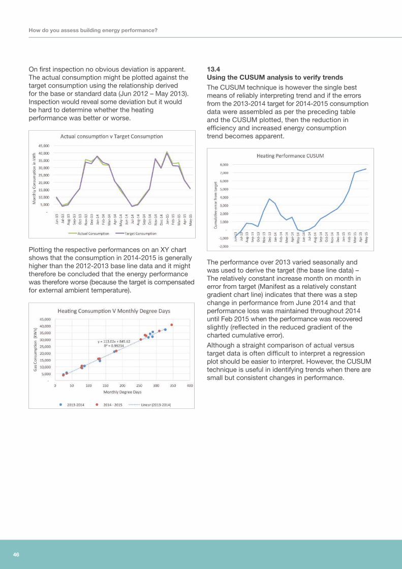
46

On first inspection no obvious deviation is apparent. The actual consumption might be plotted against the target consumption using the relationship derived for the base or standard data (Jun 2012 – May 2013). Inspection would reveal some deviation but it would be hard to determine whether the heating performance was better or worse.

Plotting the respective performances on an XY chart shows that the consumption in 2014-2015 is generally higher than the 2012-2013 base line data and it might therefore be concluded that the energy performance was therefore worse (because the target is compensated for external ambient temperature).

13.4 Using the CUSUM analysis to verify trendsThe CUSUM technique is however the single best means of reliably interpreting trend and if the errors from the 2013-2014 target for 2014-2015 consumption data were assembled as per the preceding table and the CUSUM plotted, then the reduction in efficiency and increased energy consumption trend becomes apparent.

The performance over 2013 varied seasonally and was used to derive the target (the base line data) – The relatively constant increase month on month in error from target (Manifest as a relatively constant gradient chart line) indicates that there was a step change in performance from June 2014 and that performance loss was maintained throughout 2014 until Feb 2015 when the performance was recovered slightly (reflected in the reduced gradient of the charted cumulative error).

Although a straight comparison of actual versus target data is often difficult to interpret a regression plot should be easier to interpret. However, the CUSUM technique is useful in identifying trends when there are small but consistent changes in performance.


47

14.1 Energy performance certificates and energy benchmarking . . . . . . . . . . . . . . . . . . . . . . 48

14.2 Building Logbooks . . . . . . . . . . . . . . . . . . . . . . . . . . . . . . . . . . . . . . . . . . . . . . . . . . . . . . 48

14.3 What is in a Building Logbook? . . . . . . . . . . . . . . . . . . . . . . . . . . . . . . . . . . . . . . . . . . . . 48

14.4 Energy Savings Opportunity Scheme (ESOS) . . . . . . . . . . . . . . . . . . . . . . . . . . . . . . . . . 49

14.0 Energy Performance in Buildings - Key Legislative Changes

48

Energy Performance in Buildings - Key Legislative Changes

In 2009 buildings accounted for about 43% of all the UK’s carbon emissions. The Government has introduced legislation to reduce carbon emissions from buildings and make sure that planning policies help to protect and improve the natural and built environment.

The Government has included policies in the National Planning Policy Framework to explain how developments should be planned to reduce carbon emissions and protect the environment.

To reduce carbon emissions from buildings, the Government:

• are requiring local planning authorities to make sure that new developments are energy efficient.

• will require all new homes to be zero carbon from 2016 and are considering extending this to include all other buildings from 2019.

• have introduced the green deal to enable people to pay for home improvements over time using savings on their regular energy bills.

• have improved Energy Performance Certificates to make them more informative and user-friendly. The 2010 Directive (2010/31/EU) has been implemented in Northern Ireland through the Energy Performance of Buildings (Certificates and Inspections) (Amendment) Regulations (Northern Ireland) 2013. These regulations amend the 2008 Regulations to implement Articles 4, 11, 12, 13, 16 and 27 of the 2010 Directive. The Energy Performance of Buildings (Certificates and Inspections) (Amendment) Regulations (Northern Ireland) 2014 , which came into operation on 25 February 2014, implement Articles 2(9), 11(2)(a), 11(2)(b), 11(3) and 13(2) of the Directive.

• have introduced the Code for Sustainable Homes which provides a single national standard for the design and construction of sustainable new homes.

14.1 Energy performance certificates and energy benchmarkingThe Department for Communities and Local Government (DCLG) is responsible for making sure buildings in the UK meet the standards required by the EU’s Energy Performance of Buildings Directive.

The Directive requires that:

• all properties (homes, commercial and public buildings) must have an Energy Performance Certificate (EPC) when sold, built or rented.

• larger public buildings over 500m² must display a Display Energy Certificate (DEC)

• all air-conditioning systems over 12kW must be regularly inspected by an Energy Assessor.

EPCs are produced by accredited energy assessors using standard methods and assumptions about energy usage. This means that the energy efficiency of one building can easily be compared with another building of the same type. This allows prospective buyers, tenants, owners, occupiers and purchasers to see information on the energy efficiency and carbon emissions from their building so they can consider energy efficiency and fuel costs as part of their investment.

An EPC includes a recommendation report that lists cost-effective and other measures to improve the building’s energy rating.

14.2 Building logbooksBuilding Logbooks are legally required for new commercial buildings and for existing buildings where the building services provision is altered. The Government alleges that building logbooks will improve the information that facilities managers or building managers have in regard of building energy performance. The theory is that building managers will then be able to influence the energy performance of the building – In practice building managers may not be qualified, experienced or able to programme the services control systems. However, buildings logbooks will allow ongoing building energy performance, to be recorded.

The theory is that logbooks will improve the understanding, management and operation of buildings resulting in lower costs and reduced carbon dioxide (C02) whilst contributing to improved comfort, and productivity.

14.3 What is in a Building Logbook?The logbook should provide access to information on the design, commissioning and energy consumption of the building. Again in theory, it is intended that a building manager will be able to manage controls and settings to improve energy efficiency.

The log book will also provide detailed information about metering strategies implemented in the building and the scope for monitoring and benchmarking energy consumption.

49

Energy Performance in Buildings - Key Legislative Changes

CIBSE TM31: Building Logbooks an Authors guide

GPG348 ‘Building logbooks a users guide’ available at www.thecarbontrust.co.uk

14.4 Energy Savings Opportunity Scheme (ESOS)ESOS (Energy Savings Opportunity Scheme) presents a new significant opportunity for large UK businesses.

The ESOS is a mandatory scheme for large organisations in the UK. It requires organisations to undertake a regular assessment to identify cost effective energy savings measures. This scheme was established by the Department of Energy and Climate Change (DECC) in response to the requirement for all Member States of the European Union to implement Article 8 of the Energy Efficiency Directive.

50

15.0 Other Useful Reading

51

Other Useful Reading

Monitoring and targeting (Carbon Trust Guide)www.carbontrust.com/media/31683/ctg008_monitoring_and_targeting.pdf

Energy Efficiency in Buildings CIBSE Guide F

Statistical Process Control: Theory and Practice (Wetherhill and Brown) Textbook

If you require this leaflet in an alternative format (including Braille, audio disk, large print or in minority languages to meet the needs of those whose first language is not English) then please contact:

Invest NI Equality Team T : 028 9069 8273 Text Relay Number : 18001 028 9069 8273 E-mail : [email protected]

Bedford Square Bedford Street Belfast BT2 7ES T : 028 9069 8000 F : 028 9043 6536 Text Relay Number: 18001 028 9069 8000

investni.com

Documents

Metering, Monitoring and Targeting - Invest Northern … · 2.0 What is Metering, Monitoring and Targeting ... 3.3 Improved product costing ... 4.5 A system for analysis