Embed Size (px)
Citation preview

Method B Bacteroidales in Water by TaqManreg Quantitative Polymerase Chain Reaction (qPCR) Assay
June 2010
Note that this method will be updated following its validation in marine and fresh ambient waters
US Environmental Protection Agency Office of Water (4303T)
1200 Pennsylvania Avenue NW Washington DC 20460
EPA-822-R-10-003
Acknowledgments
This method was developed under the direction of Rich Haugland Kevin Oshima and Alfred P Dufour of the US Environmental Protection Agencyrsquos (EPA) Human Exposure Research Division National Exposure Research Laboratory Cincinnati Ohio Screen shots for the ABI 7500 and the Smart Cyclerreg (Software version 20) were kindly provided by Jack Paar III of EPArsquos New England Regional Laboratory
The following laboratories are gratefully acknowledged for their participation in the single laboratory validation of this method in fresh and marine waters
Participant Laboratories
bull New York State Department of Health Environmental Biology Laboratory Ellen Braun-Howland and Stacey Chmura
bull Mycometrics LLC King-Teh Lin and Pi-shiang Lai
iii
Disclaimer
Neither the United States Government nor any of its employees contractors or their employees make any warranty expressed or implied or assumes any legal liability or responsibility for any third partyrsquos use of apparatus product or process discussed in this method or represents that its use by such party would not infringe on privately owned rights Mention of trade names or commercial products does not constitute endorsement or recommendation for use
Questions concerning this method or its application should be addressed to
Robin K Oshiro Engineering and Analysis Division (4303T) US EPA Office of Water Office of Science and Technology 1200 Pennsylvania Avenue NW
Washington DC 20460 oshirorobinepagov or OSTCWAMethodsepagov
iv
Introduction
Bacteria of the Bacteroidales order are commonly found in the feces of humans and other warm-blooded animals Although these organisms can be persistent in the environment the presence of Bacteroidales in water is an indication of fecal pollution and the possible presence of enteric pathogens
Method B describes a quantitative polymerase chain reaction (qPCR) procedure for the detection of DNA from Bacteroidales bacteria in ambient water matrices based on the amplification and detection of a specific region of the 16S ribosomal RNA gene from these organisms Results can be obtained by this method in 3-4 hours allowing same-day notification of recreational water quality Recent epidemiological studies at fresh water recreational beaches (Reference 177) have demonstrated similar or improved positive correlations between Bacteroidales DNA measurements by this method and swimming-associated gastrointestinal (GI) illness rates
In Method B water samples are filtered to collect Bacteroidales on polycarbonate membrane filters Following filtration total DNA is solubilized from the filter retentate using a bead beater Bacteroidales target DNA sequences present in the clarified homogenate are detected by the real time polymerase chain reaction technique using TaqManreg Universal Master Mix PCR reagent and the TaqManreg probe system The TaqManreg system signals the formation of PCR products by a process involving enzymatic hydrolysis of a fluorogenically-labeled oligonucleotide probe when it hybridizes to the target sequence
Method B uses an arithmetic formula the comparative cycle threshold (CT) method to calculate the ratio of Bacteroidales 16S rRNA gene target sequences (target sequences) recovered in total DNA extracts from water samples relative to those in similarly-prepared extracts of calibrator samples containing a known quantity of Bacteroidales cells Mean estimates of the absolute quantities of target sequences in the calibrator sample extracts are then used to determine the absolute quantities of target sequences in the water samples CT values for sample processing control (SPC) sequences added in equal quantities to both the water filtrate and calibrator samples before DNA extraction are used to normalize results for potential differences in DNA recovery or to signal inhibition or fluorescence quenching of the PCR analysis caused by a sample matrix component or possible technical error
v
Table of Contents
10 Scope and Application
1
20 Summary of Method 1
30 Definitions 1
40 Interferences 2
50 Safety 3
60 Equipment and Supplies
3
70 Reagents and Standards 5
80 Sample Collection Handling and Storage 9
90 Quality Control 9
100 Calibration and Standardization of Method-Related Instruments 12
110 Procedure
12
120 Data Analysis and Calculations 21
130 Sample Spiking Procedure 24
140 Method Performance 25
150 Pollution Prevention 25
160 Waste Management
25
170 References 26
180 Acronyms 26
vi
List of Appendices Appendix A ABI 7900 and ABI 7500 Sequence Detector Operation Appendix B Cepheid Smart Cyclerreg Operation
vii
Method B Bacteroidales in Water by Quantitative Polymerase Chain Reaction (qPCR) Assay
June 2010
10 Scope and Application
11 Method B describes a quantitative polymerase chain reaction (qPCR) procedure for the measurement of the 16S ribosomal RNA (16S rRNA) target gene sequences from all known bacteria of the order Bacteroidales in water This method is based on the collection of Bacteroidales on membrane filters extraction of total DNA using a bead beater and detection of Bacteroidales target sequences in the supernatant by real time polymerase chain reaction using TaqManreg Universal Master Mix PCR reagent and the TaqManreg probe system The TaqManreg system signals the formation of PCR products by a process involving the enzymatic hydrolysis of a labeled fluorogenic probe that hybridizes to the target sequence
12 Bacteroidales are commonly found in the feces of humans and other warm-blooded animals Although DNA from these organisms can be persistent in the environment its presence in water is an indication of fecal pollution and the possible presence of enteric pathogens
13 The Method B test is recommended as a measure of ambient fresh and marine recreational water quality Epidemiological studies have been conducted at fresh water and marine water beaches that may lead to the potential development of criteria that can be used to promulgate recreational water standards based on established relationships between health effects and water quality measurements by this method The significance of finding Bacteroidales DNA target sequences in recreational water samples stems from the direct relationship between the density of these sequences and the risk of gastrointestinal illness associated with swimming in the water that have been observed thus far in the epidemiological studies (Reference 177)
14 This method assumes the use of an ABI sequence detector as the default platform The Cepheid Smart Cyclerreg may also be used The user should refer to the platform specific instructions for these instruments in the Appendices Users should thoroughly read the method in its entirety before preparation of reagents and commencement of the method to identify differences in protocols for different platforms
20 Summary of Method
The method is initiated by filtering a water sample through a membrane filter Following filtration the membrane containing the bacterial cells and DNA is placed in a microcentrifuge tube with glass beads and buffer and then agitated to extract the DNA into solution The clarified supernatant is used for PCR amplification and detection of target sequences using the TaqManreg Universal Master Mix PCR reagent and probe system
30 Definitions
31 Bacteroidales all genera and species of the order Bacteroidales for which 16S rRNA gene nucleotide sequences were reported in the GenBank database (httpwwwncbinlmnihgovGenbank) at the time of method development
1
Method B
32 Target sequence A segment of the 16S rRNA gene containing nucleotide sequences that are homologous to both the primers and probe used in the Bacteroidales qPCR assay and that are common only to species within this order
33 Sample processing control (SPC) sequence (may also be referred to as reference sequence) A segment of the ribosomal RNA gene operon internal transcribed spacer region 2 of chum salmon Oncorhynchus keta (O keta) containing nucleotide sequences that are homologous to the primers and probe used in the SPC qPCR assay SPC sequences are added as part of a total salmon DNA solution in equal quantities to all water sample filtrate and calibrator samples prior to extracting DNA from the samples
34 DNA standard A purified RNA-free and spectrophotometrically quantified and characterized Bacteroides thetaiotaomicron strain ATCC 29741 genomic DNA preparation DNA standards are used to generate standard curves for determination of performance characteristics of the qPCR assays and instrument with different preparations of master mixes containing TaqManreg reagent primers and probe as described in Section 96 Also used for quantifying target sequences in calibrator sample extracts as described in Section 122
35 Calibrator sample Samples containing constant added quantities of B thetaiotaomicron strain ATCC 29741 cells and SPC sequences that are extracted and analyzed in the same manner as water samples Calibrator sample analysis results are used as positive controls for the Bacteroidales target sequence and SPC qPCR assays and as the basis for target sequence quantification in water samples using the ΔΔCT or ΔCT comparative cycle threshold calculation method as described in Section 124 Analysis results of these samples provide corrections for potential daily or weekly method-related variations in Bacteroidales cell lysis target sequence recovery and PCR efficiency QPCR analyses for SPC sequences from these samples are also used to correct for variations in total DNA recovery in the extracts of water sample filtrates that can be caused by contaminants in these filtrates as described in Section 124 andor to signal potentially significant PCR inhibition caused by these contaminants as described in Section 98
36 ΔΔCT comparative cycle threshold calculation method (ΔΔCT method) A calculation method derived by Applied Biosystems (Reference 171) for calculating the ratios of target sequences in two DNA samples (eg a calibrator and water sample) that either controls (ΔCT method) or normalizes (ΔΔCT method) for differences in total DNA recovery from these samples using qPCR analysis CT values for a reference (SPC) sequence that is initially present in equal quantities prior to DNA extraction
37 Amplification factor (AF) A measure of the average efficiency at which target or SPC sequences are copied and detected by their respective primer and probe assays during each thermal cycle of the qPCR reaction that is used in the comparative cycle threshold calculation methods AF values can range from 1 (0 of sequences copied and detected) to 2 (100 of sequences copied and detected) and are calculated from a standard curve as described in Section 122
40 Interferences
Water samples containing colloidal or suspended particulate materials can clog the membrane filter and prevent filtration These materials can also interfere with DNA recovery and interfere with the PCR analysis by inhibiting the enzymatic activity of the Taq DNA polymerase andor inhibiting the annealing of the primer and probe oligonucleotides to sample target DNA enzyme or quenching of hydrolyzed probe fluorescence
2
Method B
50 Safety
51 The analysttechnician must know and observe the normal safety procedures required in a microbiology andor molecular biology laboratory while preparing using and disposing of cultures reagents and materials and while operating sterilization equipment
52 Where possible facial masks should be worn to prevent sample contamination
53 Mouth-pipetting is prohibited
60 Equipment and Supplies
61 Separated and dedicated workstations for reagent preparation and for sample preparation preferably with HEPA-filtered laminar flow hoods and an Ultraviolet (UV) light source each having separate supplies (eg pipettors tips gloves etc) Note The same workstation may be used for the entire procedure provided that it has been cleaned with bleach and UV sterilized as specified in section 1161 between reagent and sample preparation Under ideal conditions two dedicated workstations are used for sample preparation one for preparing samples with high target sequence DNA concentrations (eg DNA standards and calibrator samples) and one for preparing samples with expected low target sequence DNA concentrations (eg filter blanks and ambient water samples)
62 Balance capable of accuracy to 001 g
63 Extraction tubes semi-conical screw cap microcentrifuge tubes 20-mL (eg PGC 506-636 or equivalent)
64 Glass beads acid washed 212 - 300 μm (eg Sigma G-1277 or equivalent)
65 Autoclave capable of achieving and maintaining 121degC [15 lb pressure per square inch (PSI)] for minimally 15 minutes
66 Workstation for water filtrations preferably a HEPA-filtered laminar flow hood with a UV light source This can be the same as used for sample preparation Section 61
67 Sterile bottlescontainers for sample collection
68 Membrane filtration units (filter base and funnel) for 47 mm diameter filters sterile glass plastic (eg Pall Gelman 4242 or equivalent) stainless steel or disposable plastic (eg Nalgene CN 130-4045 or CN 145-0045 or equivalent) cleaned and bleach treated (rinsed with 10 vv bleach then 3 rinses with reagent-grade water) covered with aluminum foil or Kraft paper and autoclaved or UV-sterilized if non-disposable
69 Line vacuum electric vacuum pump or aspirator for use as a vacuum source In an emergency or in the field a hand pump or a syringe equipped with a check valve to prevent the return flow of air can be used
610 Flask filter vacuum usually 1 L with appropriate tubing
611 Filter manifold to hold a number of filter bases
612 Flask for safety trap placed between the filter flask and the vacuum source
613 Anaerobic chamber (BD BBL GasPak 150 Jar System or equivalent)
614 Disposable gas generator pouches (BD BBL Gas Pak Plus Hydrogen or equivalent)
3
Method B
615 Forceps straight or curved with smooth tips to handle filters without damage 2 pairs
616 Polycarbonate membrane filters sterile white 47 mm diameter with 045 Fm pore size (eg GE Osmotics Inc 04CP04700 or equivalent)
617 Graduated cylinders 100-1000-mL cleaned and bleach treated (rinsed with 10 vv bleach then 3 rinses with reagent-grade water) covered with aluminum foil or Kraft paper and autoclaved or UV-sterilized
618 Petri dishes sterile plastic or glass 100 times 15 mm with loose fitting lids
619 Disposable loops 1 and 10 μL
620 Sterile 1cc syringes
621 Sterile 2rdquo needles 18 gauge
622 Permanent ink marking pen for labeling tubes
623 Visible wavelength spectrophotometer capable of measuring at 595 nm
624 Single or 8-place mini bead beater (eg Biospec Products Inc 3110BX or equivalent)
625 Microcentrifuge capable of 12000 times g
626 Micropipettors with 10 20 200 and 1000 μL capacity Under ideal conditions each workstation should have a dedicated set of micropipettors (one micropipettor set for pipetting reagents not containing cells or reference DNA and one set for reagents containing reference DNA and for test samples)
627 Micropipettor tips with aerosol barrier for 10 20 200 and 1000 μL capacity micropipettors Note All micropipetting should be done with aerosol barrier tips The tips used for reagents not containing DNA should be separate from those used for reagents containing DNA and test samples Each workstation should have a dedicated supply of tips
628 Microcentrifuge tubes low retention clear 17-mL (eg GENE MATE C-3228-1 or equivalent )
629 Test tube rack for microcentrifuge tubes use a separate rack for each set of tubes
630 Conical centrifuge tubes sterile screw cap 50-mL
631 Test tubes screw cap borosilicate glass 16 times 125 mm
632 Pipet containers stainless steel aluminum or borosilicate glass for glass pipets
633 Pipets sterile TD bacteriological or Mohr disposable glass or plastic of appropriate volume (disposable pipets preferable)
634 Vortex mixer (ideally one for each work station)
635 Dedicated lab coats for each work station
636 Disposable powder-free gloves for each work station
637 Refrigerator 4degC (ideally one for reagents and one for DNA samples)
638 Freezer -20degC or -80degC (ideally one for reagents and one for DNA samples)
639 Ice crushed or cubes for temporary preservation of samples and reagents
640 Printer (optional)
641 Data archiving system (eg flash drive or other data storage system)
4
Method B
642 UV spectrophotometer capable of measuring wavelengths of 260 and 280 nm using small volume capacity (eg 01 mL) cuvettes or NanoDropreg (ND-1000) spectrophotometer (or equivalent) capable of the same measurements using 2 μL sample volumes
643 ABI 7900 or ABI 7500 Sequence Detector
6431 Optical 96 well PCR reaction tray (eg Applied Biosystems N801-0560 or equivalent)
6432 Optical adhesive PCR reaction tray tape (eg Applied Biosystems 4311971 or equivalent) or MicroAmptrade caps (eg Applied Biosystems N8010534 or equivalent)
6433 ABI 7900 sequence detector
644 Cepheid Smart Cyclerreg
6441 Smart Cyclerreg 25 μL PCR reaction tubes (eg Cepheid 900-0085 or equivalent)
6442 Rack and microcentrifuge for Smart Cyclerreg PCR reaction tubes Note Racks and microcentrifuge are provided with the Smart Cyclerreg thermocycler
6443 Cepheid Smart Cyclerreg System Thermocycler
70 Reagents and Standards Note The Bacteroidales stock culture (Section 79) Salmon DNAextraction buffer (Section 713) and DNA extraction tubes (Section 719) may be prepared in advance
71 Purity of Reagents Molecular-grade reagents and chemicals shall be used in all tests
72 Control Culture
bull Bacteroides thetaiotaomicron (B thetaiotaomicron) ATCC 29741
73 Sample Processing Control (SPC) DNA (source of SPC control sequences)
bull Salmon testes DNA (eg Sigma D1626 or equivalent)
74 Phosphate Buffered Saline (PBS)
741 Composition
Monosodium phosphate (NaH2PO4) 058 g Disodium phosphate (Na2HPO4) 250 g Sodium chloride 850 g Reagent-grade water 10 L
742 Dissolve reagents in 1 L of reagent-grade water in a flask and dispense in appropriate amounts for dilutions in screw cap bottles or culture tubes andor into containers for use as reference matrix samples and rinse water Autoclave after preparation at 121degC [15 lb pressure per square inch (PSI)] for 15 minutes Final pH should be 74 plusmn 02
75 Chopped Meat Carboyhydrates Broth (CMCB) Note Formulation is provided only to ensure that the appropriate medium is used for analyses laboratories should use commercially prepared tubes
Note Pre-mixed powder forms of this medium are not available
751 Composition
5
Method B
Chopped Meat Pellets 102 g Pancreatic Digest of Casein 300 g Yeast extract 50 g Glucose 40 g Dipotassium Phosphate 50 g Cellobiose 10 g Maltose 10 g Starch 10 g L-Cysteine HCl 05 g Resazurin 0001 g Vitamin K1 10 mg Hemin 50 mg Reagent-grade water 10 L
752 This medium is manufactured in a pre-reduced (oxygen-free) environment and sealed to prevent aerobiosis The medium is pre-sterilized and ready for inoculation
76 CDC Anaerobe 5 Sheep Blood (BAP) Note Formulation is provided only to ensure that the appropriate medium is used for analyses laboratories should use commercially prepared plates
761 Composition
Pancreatic Digest of Casein 150 g
Papaic Digest of Soybean Meal 50 g
Sodium Chloride 50 g
Agar 200 g
Yeast Extract 50 g Hemin 0005 g
Vitamin K1 001 g
L-Cystine 04 g
Reagent-grade water 1 L
Defibrinated Sheep Blood 5
77 Sterile glycerol (used for preparation of B thetaiotaomicron stock culture as described in section 79)
78 Preparation of B thetaiotaomicron (ATCC 29741) stock culture
Rehydrate lyophilized B thetaiotaomicron per manufacturerrsquos instructions (for ATCC stocks suspend in 05 mL of sterile chopped meat carbohydrate broth (CMCB) and mix well to dissolve lyophilized culture Using a sterile syringe and needle aspirate suspension and inoculate 10 mL of CMCB Incubate at 350degC plusmn 05degC for 24-72 hours After incubation remove septum and transfer liquid to a sterile tube by pipetting While pipetting the suspension use extreme care to remove as much liquid as possible without siphoning any particulates Centrifuge suspension at
6
Method B
6000 x g for 5 minutes to create a cell pellet Using a sterile pipet discard supernatant Resuspend pellet in 10 mL of fresh sterile CMCB without the particulates containing 15 glycerol and dispense in 15-mL aliquots in microcentrifuge tubes Freeze at -20degC (short term storage) or -80degC (long term storage) Note Aliquots of suspension may be plated to determine CFU concentration as described in Section 111 It is advisable to verify the B thetaiotaomicron culture by using commercially available test kits (eg Vitekreg or APIreg)
79 PCR-grade water (eg OmniPur water from VWR EM-9610 or equivalent) Water must be DNADNase free
710 Isopropanol or ethanol 95 for flame-sterilization
711 AE Buffer pH 90 (eg Qiagen 19077 or equivalent) (Note pH 80 is acceptable)
Composition
10 mM Tris-Cl (chloride)
05 mM EDTA (Ethylenediaminetetraacetic acid)
712 Salmon DNAextraction buffer
7121 Composition
Stock Salmon testes DNA (10 μgmL) (Section 73)
AE Buffer (Section 712)
7122 Preparation of stock Salmon testes DNA Each bottle of Salmon DNA contains a specific number of units Note the units Add an equal volume of PCR-grade water to dissolve the Salmon testes DNA and stir using a magnetic stir bar at low to medium speed until dissolved (2-4 hours if necessary) The solution at this point will be equivalent to 50 μg Salmon testes DNAmL Dilute using PCR grade water to a concentration of ~ 10 μgmL Determine concentration of Salmon testes DNA stock by OD260 reading in a spectrophotometer An OD260 of 1 is approximately equal to 50 μgmL (one Unit) This is your Salmon testes DNA stock solution Unused portion may be aliquoted and frozen at 20degC
Note For example if the bottle contains 250 mg of DNA using sterilized scissors and sterilized forceps cut a piece of DNA to weigh approximately 20 mg (approximately 304 Units) and place in a sterile weigh boat After weighing place the DNA into a sterile 50 mL tube and add 20 mL PCR grade water Cap tightly and resuspend by 2-4 hours of gentle rocking The concentration should be about 1 mgmL Remove three 10 μL aliquots and dilute each to 1 mL with PCR grade water Check absorbance (OD260) and calculate DNA using the assumption 1 Unit DNA is equal to 1 OD260 which is then equivalent to 50 μgmL DNA Adjust this stock to 10 μgmL based on calculated initial concentration of 1 mgmL by diluting with PCR grade water Aliquot portions of the adjusted DNA stock and freeze
7123 Dilute Salmon testes DNA stock with AE buffer to make 02 μgmL Salmon DNAextraction buffer Extraction buffer may be prepared in advance and stored at 4deg C for a maximum of 1 week
Note Determine the total volume of Salmon DNAextraction buffer required for each day or week by multiplying volume (600 μL) times total number of samples to be analyzed including controls water samples and calibrator samples For example for 18 samples prepare enough SalmonDNA extraction buffer for 24 extraction tubes (18divide6 = 3 therefore 3 extra tubes for water sample filtration blanks (method blanks) and 3 extra
7
Method B
tubes for calibrator samples) Note that the number of samples is divided by 6 because you should conduct one method blank for every 6 samples analyzed Additionally prepare excess volume to allow for accurate dispensing of 600 μL per tube generally 1 extra tube Thus in this example prepare sufficient SalmonDNA extraction buffer for 24 tubes plus one extra The total volume needed is 600 μL times 25 tubes = 15000 μL Dilute the Salmon testes DNA working stock 150 for a total volume needed (15000 μL) divide 50 = 300 μL of 10 μgmL Salmon testes DNA working stock The AE buffer needed is the difference between the total volume and the Salmon testes DNA working stock For this example 15000 μL - 300 μL = 14700 μL AE buffer needed
713 Bleach solution 10 vv bleach (or other reagent that hydrolyzes DNA) (used for cleaning work surfaces)
714 Sterile water (used as rinse water for work surface after bleaching)
715 TaqManreg Universal PCR Master Mix (eg Applied Biosystems 4304437 or equivalent)
Composition
AmpliTaq Goldreg DNA Polymerase
AmpErasereg UNG
dNTPs with dUTP
Passive Reference 1 (ROXtrade fluorescent dye)
Optimized buffer components (KCl Tris EDTA MgCl2)
716 Bovine serum albumin (BSA) fraction V powder eg Sigma B-4287 or equivalent)
Dissolve in PCR-grade water to a concentration of 2 mgmL
717 Primer and probe sets Primer and probe sets may be purchased from commercial sources Primers should be desalted probes should be HPLC purified
7171 Bacteroidales primer and probe set (References 174 and 176)
Forward primer 5-GGGGTTCTGAGAGGAAGGT
Reverse primer 5-CCGTCATCCTTCACGCTACT
TaqManreg probe 5-FAM-CAATATTCCTCACTGCTGCCTCCCGTA-TAMRA
7172 Salmon DNA primer and probe set (Reference 174)
Forward primer 5-GGTTTCCGCAGCTGGG
Reverse primer (Sketa 22) 5-CCGAGCCGTCCTGGTC
TaqManreg probe 5-FAM-AGTCGCAGGCGGCCACCGT-TAMRA
7173 Preparation of primerprobes Using a micropipettor with aerosol barrier tips add PCR grade water to the lyophilized primers and probe from the vendor to create stock solutions of 500 μM primer and 100 μM probe and dissolve by extensive vortexing Pulse centrifuge to coalesce droplets Store stock solutions at -20degC
718 DNA extraction tubes
Note It is recommended that tube preparation be performed in advance of water sampling and DNA extraction procedures
Prepare 1 tube for each sample and 1 extra tube for every 6 samples (ie for method blank) and minimum of 3 tubes per week for calibrator samples Weigh 03 plusmn 001 g of glass beads (Section
8
Method B
64) and pour into extraction tube Seal the tube tightly checking to make sure there are no beads on the O-ring of the tube Check the tube for proper O-ring seating after the tube has been closed Autoclave at 121degC (15 PSI) for 15 minutes
719 Purified RNA-free and spectrophotometrically quantified and characterized B thetaiotaomicron genomic DNA preparations used to generate a standard curve (see Section 112)
720 RNase A (eg Sigma Chemical R-6513) or equivalent
7201 Composition
RNase A
Tris-Cl
NaCl
7202 Dissolve 10 mgmL pancreatic RNase A in 10 mM Tris-Cl (pH 75) 15 mM NaCl Heat to 100degC for 15 minutes Allow to cool to room temperature Dispense into aliquots and store at - 20degC For working solution prepare solution in PCR-grade water at concentration of 5 μgμL
721 DNA extraction kit (Gene-Rite K102-02C-50 DNA-EZreg RW02 or equivalent)
80 Sample Collection Handling and Storage 81 Sampling procedures are briefly described below Adherence to sample preservation procedures
and holding time limits is critical to the production of valid data Samples not collected according to these procedures should not be analyzed
82 Sampling Techniques
Samples are collected by hand or with a sampling device if the sampling site has difficult access such as a dock bridge or bank adjacent to surface water Composite samples should not be collected since such samples do not display the range of values found in individual samples The sampling depth for surface water samples should be 6-12 inches below the water surface Sample containers should be positioned such that the mouth of the container is pointed away from the sampler or sample point After removal of the container from the water a small portion of the sample should be discarded to provide head space for proper mixing before analyses
83 Storage Temperature and Handling Conditions
Ice or refrigerate water samples at a temperature of lt10degC during transit to the laboratory Do not freeze the samples Use insulated containers to assure proper maintenance of storage temperature Take care that sample bottles are tightly closed and are not totally immersed in water during transit
84 Holding Time Limitations
Examine samples as soon as possible after collection Do not hold samples longer than 6 hours between collection and initiation of filtration This section will be updated based on results of holding time study
90 Quality Control
9
Method B
91 Each laboratory that uses Method B is required to operate a formal quality assurance (QA) program that addresses and documents instrument and equipment maintenance and performance reagent quality and performance analyst training and certification and records sample storage and retrieval Additional recommendations for QA and quality control (QC) procedures for microbiological laboratories are provided in Reference 172
92 Media sterility check mdash The laboratory should test media sterility by incubating one unit (tube or plate) from each batch of medium (5 BAP CMCB) as appropriate and observing for growth Absence of growth indicates media sterility On an ongoing basis the laboratory should perform a media sterility check every day that samples are analyzed
93 Method blank (water sample filtration blank) mdash Filter a 50 mL volume of sterile PBS before beginning the sample filtrations Remove the funnel from the filtration unit Using two sterile or flame-sterilized forceps fold the filter on the base of the filtration unit and place it in an extraction tube with glass beads as described in Section 720 Extract as in Section 115 Absence of fluorescence growth curve during PCR analysis of these samples (reported as ldquo0 on Smart Cyclerreg and ldquoundeterminedrdquo on ABI model 7900) indicates the absence of contaminant target DNA (see Data Quality Acceptance below) Prepare one method blank filter for every six samples
94 Positive controls mdash The laboratory should analyze positive controls to ensure that the method is performing properly Fluorescence growth curve (PCR amplification trace) with an appropriate cycle threshold (CT) value during PCR indicates proper method performance On an ongoing basis the laboratory should perform positive control analyses every day that samples are analyzed In addition controls should be analyzed when new lots of reagents or filters are used
941 Calibrator samples will serve as the positive control Analyze as described in Section 110 Note Calibrator samples contain the same amount of extraction buffer and starting amount of Salmon DNA as the test samples hence B thetaiotaomicron calibrator DNA extracts (Section 113) will be used as a positive control for both Bacteroidales and SPC qPCR assays
942 If the positive control fails to exhibit the appropriate fluorescence growth curve response check andor replace the associated reagents and reanalyze If positive controls still fail to exhibit the appropriate fluorescence growth curve response prepare new calibrator samples and reanalyze (see Section 97)
95 No template controls mdash The laboratory should analyze ldquoNo Template Controlsrdquo (NTC) to ensure that the Master Mix PCR reagents are not contaminated On an ongoing basis the laboratory should perform NTC analyses every day that samples are analyzed If greater than one-third of the NTC reactions for a PCR master mix exhibit true positive logarithmic amplification traces with CT values below 45 (not from chemical degradation of probe with linear kinetics that exhibit rising baseline) or if any one NTC reaction has a CT value lower than 35 the analyses should be repeated with new Master Mix working stock preparations
96 DNA standards and standard curves ndashPurified RNA-free and spectrophotometrically quantified B thetaiotaomicron genomic DNA should be prepared as described in Section 112 Based on reported values for it size the weight of a single B thetaiotaomicron genome can be estimated to be ~67 fg and there are six 16S rRNA gene copies per genome in this species (httpcmrjcviorgtigr-scriptsCMRsharedGenomescgi) The concentration of 16S rRNA gene copies per μL in the standard B thetaiotaomicron genomic DNA preparation can be determined from this information and from its spectrophotometrically determined total DNA concentration by the formula
10
Method B
Concentration of 16S rRNA gene copies
per μL =
Total DNA concentration (fgμL) x 6 16S rRNA gene copies
67 fggenome genome
A composite standard curve should be generated from multiple analyses of serial dilutions of this DNA standard using the Bacteroidales primer and probe assay and subjected to linear regression analysis as described in Section 122 From that point on it is recommended that additional standard curves be generated from duplicate analyses of these same diluted standard samples with each new lot of TaqManreg master mix reagents or primers and probes to demonstrate comparable performance by these new reagents The r2 values from regressions of these curves should ideally be 099 or greater Comparable performance is assessed by their slopes and y-intercepts which should be consistent with those from the initial composite analyses (eg within the 95 confidence range of the average values) Note The 95 confidence ranges for these parameters in the initial composite standard curve can be generated using the Regression Analysis Tool which can be accessed from the ldquoData Analysisrdquo selection under the ldquoToolsrdquo menu in Excel Subsequent regressions can be performed by plotting the data using the Chart Wizard in Excel and using the ldquoadd trend linerdquo selection in the Chart menu and ldquodisplay equation on chartrdquo selection under Options to obtain slope and y-intercept values as illustrated in Section 122
In the event that the slope value from a subsequent standard curve regression is outside of the acceptance range the diluted standards should be re-analyzed If this difference persists new working stocks of the reagents should be prepared and the same procedure repeated If the differences still persist the amplification factor values used for calculations of target cell numbers as described in Section 8 should be modified based on the new slope values If the slopes are within acceptance range but Y-intercepts are not within acceptance range of this previous average new serial dilutions of the DNA standard should be prepared and analyzed as described above
97 Calibrator samples mdash The cell concentration of each cultured B thetaiotaomicron stock suspension used for the preparation of calibrator sample extracts should be determined as described in Section 111 A minimum of nine calibrator sample extracts should initially be prepared from three different freezer-stored aliquots of these stocks as described in Section 112 Dilutions of each of these calibrator sample extracts equivalent to the anticipated dilutions of the test samples used for analysis (eg 1 5 andor 25 fold) should be analyzed with the Bacteroidales primer and probe assay The average and standard deviation of the CT values from these composite analyses should be determined From that point on a minimum of three fresh calibrator sample extracts should be prepared from an additional frozen aliquot of the same stock cell suspension at least weekly and preferably daily before analyses of each batch of test samples Dilutions of each new calibrator sample extract equivalent to the initial composite dilutions (eg 1 5 andor 25 fold) should be analyzed using the Bacteroidales primer and probe assay The average CT value from these analyses should not be significantly different from the laboratorys average values from analyses of the initial calibrator sample extracts from the same stock cell suspension (ie not greater than three standard deviations) If these results are not within this acceptance range new calibrator extracts should be prepared from another frozen aliquot of the same stock cell suspension and analyzed in the same manner as described above If the results are still not within the acceptance range the reagents should be checked by the generation of a standard curve as described in Section 96
98 Salmon DNA Sample Processing Control (SPC) sequence analyses mdash While not essential it is good practice to routinely prepare and analyze standard curves from serial dilutions of Salmon
11
Method B
DNA working stocks in a manner similar to that described for the B thetaiotaomicron DNA standards in Section 96 At this time rRNA gene operon copy numbers per genome have not been reported in the literature for the salmon species O keta Therefore log-transformed total DNA concentration values or dilution factor values can be substituted for target sequence copy numbers as the x-axis values in these plots and regression analyses
In general target DNA concentrations in test samples can be calculated as described in Section 12 However the Salmon DNA PCR assay results for each test samplersquos 5 fold dilution should be within 3 CT units of the mean of the 5 fold diluted calibrator (andor method blank) sample results Higher CT values may indicate significant PCR inhibition or poor DNA recovery possibly due to physical chemical or enzymatic degradation Repeat the Bacteroidales and Salmon DNA PCR assays of any samples whose 5 fold dilution exhibits a Salmon DNA PCR assay CT value greater than 3 CT units higher than the mean of the calibrator sample results using a 5 fold higher dilution (net dilution 25 fold) of the extracts The Bacteroidales PCR result from assaying the original 5-fold dilution of the sample can be accepted if its Salmon DNA assay CT value is lower than that of the corresponding 25 fold dilution of the sample This pattern of results is indicative of poor recovery of total DNA in the extract rather than PCR inhibition The poor DNA recovery is compensated for by the calculation method Contrarily if the Salmon PCR assay CT value of the 25-fold dilution of the sample is lower than that of the 5 fold dilution of the sample then the Bacteroidales PCR assay result from the 25 fold dilution of the sample is considered more accurate However the Bacteroidales PCR results should be reported as questionable if the Salmon DNA assayrsquos result is still not within 3 CT units of the mean CT result of the 25 fold dilution of the three calibrators
100 Calibration and Standardization of Method-Related Instruments 101 Check temperatures in incubators twice daily with a minimum of 4 hours between each reading to
ensure operation within stated limits
102 Check thermometers at least annually against a NIST certified thermometer or one that meets the requirements of NIST Monograph SP 250-23 Check columns for breaks
103 Spectrophotometer should be calibrated each day of use using OD calibration standards between 001 - 05 Follow manufacturer instructions for calibration
104 Micropipettors should be calibrated at least annually and tested for accuracy on a weekly basis Follow manufacturer instructions for calibration
105 Follow manufacturer instructions for calibration of real-time PCR instruments
110 Procedure Note B thetaiotaomicron cell suspensions (Section 111) and B thetaiotaomicron DNA standards (Section 112) may be prepared in advance Calibrator samples (Section 113) should be prepared at least weekly
111 Preparation of B thetaiotaomicron cell suspensions for DNA standards and calibrator samples
1111 Thaw a B thetaiotaomicron (ATCC 29741) stock culture (Section 78) and streak for isolation on CDC anaerobe 5 sheep blood agar (BAP) plates Incubate plates at 350degC plusmn 05degC for 24 plusmn 2 hours under anaerobic conditions
1112 Pick an isolated colony of B thetaiotaomicron from the BAP plates and suspend in 1 mL of sterile phosphate buffered saline (PBS) and vortex
12
Method B
1113 Use 10 μL of the 1-mL suspension of B thetaiotaomicron to inoculate a 10-mL CMCB tube Place the inoculated tube and one uninoculated tube (sterility check) in an anaerobe chamber with a Gas Pak and incubate at 350degC plusmn 05degC for 24 plusmn 2 hours Note It is advisable to verify that the selected colony is Bacteroides by using biochemical test strips or individual biochemical tests
1114 After incubation remove septum and transfer liquid to a sterile tube by pipetting While pipetting the suspension use extreme care to remove as much liquid as possible without siphoning any of the chopped meat
1115 Centrifuge the CMCB containing B thetaiotaomicron for 5 minutes at 6000 times g
1116 Aspirate the supernatant and resuspend the cell pellet in 10 mL PBS
1117 Repeat the two previous steps twice and suspend final B thetaiotaomicron pellet in 5 mL of sterile PBS Label the tube as B thetaiotaomicron undiluted stock cell suspension noting cell concentration after determination with one of the following steps
1118 Determination of calibrator sample cell concentrations based on one of the three options below
bull Option 1 Spectrophotometric absorbance ndash Remove three 01-mL aliquots of undiluted cell suspension and dilute each with 09 mL of PBS (10-1 dilution) Read absorbance at 595 nm in spectrophotometer against PBS blank (readings should range from 005 to 03 OD) Calculate cellsmL (Y) in undiluted cell suspension using the formula below where X is the average 595 nm spectrophotometer reading
Y = (1 x 10⁹ cells mL times X) 019
bull Option 2 Hemocytometer counts ndash Serially dilute 10 μL of undiluted cell suspension with PBS to 10-1 10-2 and 10-3 dilutions and determine cell concentration of 10-2 or 10-3 dilutions in a hemocytometer or Petroff Hauser counting chamber under microscope
bull Option 3 plating ndash Note BAP plates should be prepared in advance if this option is chosen For enumeration of the B thetaiotaomicron undiluted cell suspension dilute and inoculate according to the following
A) Mix the B thetaiotaomicron undiluted cell suspension by shaking or vortexing the 5 mL tube a minimum of 25 times Use a sterile pipette to transfer 10 mL of the undiluted cell suspension to 99 mL of sterile PBS use care not to aspirate any of the particulates in the medium cap and mix by vigorously shaking the bottle a minimum of 25 times This is cell suspension dilution ldquoArdquo A 10-mL volume of dilution ldquoArdquo is 10-2 mL of the original undiluted cell suspension
B) Use a sterile pipette to transfer 110 mL of cell suspension dilution ldquoArdquo to 99 mL of sterile PBS cap and mix by vigorously shaking the bottle a minimum of 25 times This is cell suspension dilution ldquoBrdquo A 10-mL volume of dilution ldquoBrdquo is 10-3 mL of the original undiluted cell suspension
C) Use a sterile pipette to transfer 110 mL of cell suspension dilution ldquoBrdquo to 99 mL of sterile PBS cap and mix by vigorously shaking the bottle a minimum of 25 times This is cell suspension dilution ldquoCrdquo A 10-mL volume of dilution ldquoCrdquo is 10-4 mL of the original undiluted cell suspension
D) Use a sterile pipette to transfer 110 mL of cell suspension dilution ldquoCrdquo to 99 mL of sterile PBS cap and mix by vigorously shaking the bottle a minimum of 25
13
Method B
E)
F)
G)
H)
I)
J)
K)
times This is cell suspension dilution ldquoDrdquo A 10-mL volume of dilution ldquoDrdquo is 10-5 mL of the original undiluted cell suspension
Use a sterile pipette to transfer 110 mL of cell suspension dilution ldquoDrdquo to 99 mL of sterile PBS cap and mix by vigorously shaking the bottle a minimum of 25 times This is cell suspension dilution ldquoErdquo A 10-mL volume of dilution ldquoErdquo is 10-6 mL of the original undiluted cell suspension
Prepare BAP (Section 76) Ensure that agar surface is dry Note To ensure that the agar surface is dry prior to use plates should be made several days in advance and stored inverted at room temperature or dried using a laminar-flow hood
Each of the following will be conducted in triplicate resulting in the evaluation of nine spread plates
bull Pipet 01 mL of dilution ldquoCrdquo onto surface of BAP plate [10-5 mL (000001) of the original cell suspension]
bull Pipet 01 mL of dilution ldquoDrdquo onto surface of BAP plate [10-6 mL (0000001) of the original cell suspension]
bull Pipet 01 mL of dilution ldquoErdquo onto surface of BAP plate [10-7 mL (00000001) of the original cell suspension]
For each spread plate use a sterile bent glass rod or spreader to distribute inoculum over surface of medium by rotating the dish by hand or on a rotating turntable
Allow inoculum to absorb into the medium completely
Invert plates and incubate in an anaerobe chamber at 350degC plusmn 05degC for 24 plusmn 4 hours
Count and record number of colonies per plate Refer to the equation below for calculation of undiluted cell suspension concentration
CFUmLundiluted =CFU1 + CFU2 + + CFUn
V1 + V2 + + Vn
Where
CFUmLundiluted = B thetaiotaomicron CFUmL in undiluted cell suspension CFU = number of colony forming units from BAP plates yielding
counts within the ideal range of 30 to 300 CFU per plate V = volume of undiluted sample in each BAP plate yielding
counts within the ideal range of 30 to 300 CFU per plate n = number of plates with counts within the ideal range
14
Method B
Table 1 Example Calculations of B thetaiotaomicron Undiluted Cell Suspension Concentration
Examples CFU plate (triplicate analyses) from
BAP plates B thetaiotaomicron CFU mL in
undiluted suspensiona
10-5 mL plates 10-6 mL plates 10-7 mL plates
Example 1 275 250 301 30 10 5 0 0 0 (275+250+30) (10-5+10-5+10-6) = 555 (21 x 10-5) = 26428571 =
26 x 107 CFU mL
Example 2 TNTCb TNTC TNTC TNTC 299 TNTC 12 109 32
(299+109+32) (10-6+10-7+10-7) = 440 (12 x 10-6) =366666667 =
37 x 108 CFU mL
a Cell concentration is calculated using all plates yielding counts within the ideal range of 30 to 300 CFU per plate b Too numerous to count
1119 Divide remainder of undiluted cell suspension (approximately 5 mL) into 6 times 05 mL aliquots for DNA standard preparations and 100-200 times 001 mL (10 FL) aliquots for calibrator samples and freeze at 20degC Note Cell suspension should be stirred while aliquoting It is also recommended that separate micropipettor tips be used for each 10 FL aliquot transfer and that the volumes in each tip be checked visually for consistency
112 Preparation of B thetaiotaomicron genomic DNA standards
1121 Remove two 05 mL undiluted B thetaiotaomicron cell suspensions (Section 1118) from freezer and thaw completely
1122 Transfer cell suspensions to extraction tubes with glass beads
1123 Tightly close the tubes making sure that the O-rings are seated properly
1124 Place the tubes in bead beater and shake for 60 seconds at the maximum rate (5000 rpm)
1125 Remove the tubes from the bead beater and centrifuge at 12000 times g for one minute to pellet the glass beads and debris
1126 Using a 200 μL micropipettor transfer 350 μL of supernatants to sterile 17 mL microcentrifuge tubes Recover supernatants without disrupting the glass beads at the tube bottom
1127 Centrifuge crude supernatants at 12000 times g for 5 minutes and transfer 300 μL of clarified supernatant to clean labeled 17 mL low retention microcentrifuge tubes taking care not to disturb the pellet
1128 Add 1 μL of 5 μgμL RNase A solution to each clarified supernatant mix by vortexing and incubate at 37degC for 1 hour
Note Sections 1129 - 11215 may be substituted with an optional method if a DNA purification procedure is chosen other than the DNA-EZ purification kit In such a case manufacturer instructions should be followed rather than these steps Continue onward from Section 11216
1129 Add 06 mL of binding buffer solution from a DNA-EZ purification kit to each of the RNase A-treated extracts and mix by vortexing Note In general a minimum concentration of 5 x 10⁸ cells is required for this step
15
Method B
11210 If using the DNA-EZ purification kit perform the following steps Insert one DNAsuretrade column from the DNA-EZ purification kit into a collection tube (also provided with kit) for each of the two extracts Transfer the extract and binding buffer mixtures from Section 1129 to a DNAsuretrade column and collection tube assembly and centrifuge for 1 min at 12000 times g
11211 Transfer each of the DNAsuretrade columns to new collection tubes Discard previous collection tubes and collected liquid
11212 Add 500 μL EZ-Wash Buffer from the DNA-EZ purification kit to each of the DNAsuretrade columns and centrifuge at 12000 times g for 1 minute Discard the liquid in the collection tube
11213 Repeat Section 11212
11214 Transfer each of the DNAsuretrade columns to a clean labeled 17-mL low retention microcentrifuge tube and add 50 μL of DNA elution buffer to each column Centrifuge for 30 seconds at 12000 times g Repeat this procedure again to obtain a total DNA eluate volume of ~100 μL from each column
11215 Pool the two eluates to make a total volume of approximately 200 μL
11216 Transfer entire purified DNA eluate volume from each column to a clean and sterile microcuvette for UV spectrophotometer and read absorbance at 260 and 280 nM (Note the cuvette should be blanked with DNA elution buffer before reading sample) If necessary the sample may be diluted with elution buffer to reach minimum volume that can be accurately read by the spectrophotometer (see manufacturerrsquos recommendation) however this may reduce the DNA concentration to a level that can not be accurately read by the spectrophotometer If available readings can be taken of 2 μL aliquots of the sample with a NanoDroptrade Spectrophotometer
11217 Sample is acceptable as a standard if ratio of OD260OD280 readings is ge to 175
11218 Calculate total DNA concentration in sample by formula
OD260 reading x 50 ngμL DNA1(OD260)
11219 Transfer sample back to labeled 17 mL non-retentive microcentrifuge tube and store at -20degC
113 Extraction of B thetaiotaomicron calibrator samples
1131 A minimum of three calibrator extracts should be prepared during each week of analysis
Note To prevent contamination of water sample filtrates and filter blanks this procedure should be performed at a different time and if possible in a different work station than the procedures in Sections 111 and 112 above and Section 115 below
1132 Remove one tube containing a 10 μL aliquot of B thetaiotaomicron undiluted stock cell suspension (Section 1118) from the freezer and allow to thaw completely on ice
Note If using BioBalls for calibrators add a single BioBalltrade to each of 3 100 mL sterile PBS blanks filter (Section 114) and extract according to (Section 115)
1133 While cell stock is thawing using sterile (or flame-sterilized) forceps place one polycarbonate filter (Section 614) in an extraction tube with glass beads Prepare one filter for each sample to be extracted in this manner
16
Method B
1134 Dispense 590 μL of Salmon DNAextraction buffer (Section 712) into three extraction tubes with glass beads and filters Prepare one tube for each of the three calibrator samples to be extracted in this manner Label tubes appropriately
1135 When B thetaiotaomicron suspension has thawed transfer 990 μL AE buffer (Section 711) to the 10 μL B thetaiotaomicron stock cell tube and mix thoroughly by vortexing Pulse microcentrifuge tube briefly (1-2 sec) to coalesce droplets in tube
1136 Immediately after vortexing the B thetaiotaomicron suspension spot 10 μL onto the polycarbonate filter in a calibrator sample tube
1137 Tightly close the tube making sure that the O-ring is seated properly
1138 Repeat Sections 1136 and 1137 for the other two filters to prepare three calibrator samples with B thetaiotaomicron
1139 Place the tubes in the mini bead beater and shake for 60 seconds at the maximum rate (5000 rpm)
11310 Remove the tubes from the mini bead beater and centrifuge at 12000 times g for one minute to pellet the glass beads and debris
11311 Using a 200 μL micropipettor transfer the crude supernatant to the corresponding labeled sterile 17-mL microcentrifuge tube Transfer 400 μL of supernatant without disrupting the debris pellet or glass beads at the tube bottom Note The filter will normally remain intact during the bead beating and centrifugation process Generally 400 μL of supernatant can be easily collected Collect an absolute minimum of 100 μL of supernatant
11312 Centrifuge at 12000 times g for 5 minutes and transfer clarified supernatant to a clean labeled 17 mL tube taking care not to disturb the pellet Note Cell pellet may not be visible in calibrator samples
11313 Label the tubes as undiluted or 1x B thetaiotaomicron calibrator extracts Label additional 17 mL tubes for 5 and 25 fold dilutions In appropriately labeled tubes using a micropipettor add a 50 μL aliquot of each 1x B thetaiotaomicron calibrator extract and dilute each with 200 μL AE buffer (Section 711) to make 5 fold dilutions In appropriately labeled tubes using a micropipettor add a 50 μL aliquot of each 5 fold dilution and dilute each with 200 μL AE buffer to make 25 fold dilutions Store all diluted and undiluted extracts in refrigerator
11314 If the extracts are not analyzed immediately refrigerate For long term storage freeze at -80degC
114 Water sample filtration
Note It is required that one water sample filtration blank (method blank) be prepared for every 6 water samples (Section 93) analyzed by the same procedure
1141 Place a polycarbonate filter (Section 616) on the filter base and attach the funnel to the base so that the membrane filter is now held between the funnel and the base
1142 Shake the sample bottle vigorously 25 times to distribute the bacteria uniformly and measure 100 mL of sample into the funnel
1143 Filter 100 mL of water sample After filtering the sample rinse the sides of the funnel with 20-30 mL of sterile PBS (Section 74) and continue filtration until all liquid has been pulled through the filter Turn off the vacuum and remove the funnel from the filter base
17
Method B
1144 Label an extraction tube with glass beads (Section 719) to identify water sample Leaving the filter on the filtration unit base fold into a cylinder with the sample side facing inward being careful to handle the filter only on the edges where the filter has not been exposed to the sample Insert the rolled filter into the labeled extraction tube with glass beads Prepare one filter for each sample filtered in this manner
1145 Cap the extraction tube Tubes may be frozen at -20degC or -80degC until analysis
115 DNA extraction of water sample filtrates and method blanks
1151 Using a 1000 μL micropipettor dispense 590 μL of the Salmon DNAextraction buffer (Section 713) to each labeled extraction tube with glass beads containing water sample or method blank filters from Section 1144 Extract the method blank last
1152 Tightly close the tubes making sure that the O-ring is seated properly
1153 Place the tubes in the mini bead beater and shake for 60 seconds at the maximum rate (5000 rpm)
1154 Remove the tubes from the mini bead beater and centrifuge at 12000 times g for 1 minute to pellet the glass beads and debris Note To further prevent contamination a new pair of gloves may be donned for steps 1155 1156 and 1157 below
1155 Using the 200 μL micropipettor transfer 400 μL of the supernatant to a corresponding labeled sterile 17-mL microcentrifuge tube taking care not to pick up glass beads or sample debris (pellet) Note The filter will normally remain intact during the bead beating and centrifugation process Generally 400 μL of supernatant can easily be collected Collect an absolute minimum of 100 microL of supernatant Recover the method blank supernatant last
1156 Centrifuge crude supernatant from Section 1155 for 5 minutes at 12000 times g Transfer 350 μL of the clarified supernatant to another 17-mL tube taking care not to disturb pellet Note Pellet may not be visible in water samples Recover the method blank supernatant last
1157 Label the tubes from Section 1156 as undiluted or 1x water sample extracts with sample identification These are the water sample filter extracts Also label tubes for method blanks Label additional 17 mL tubes for 5 and 25 fold dilutions In appropriately labeled tubes using a micropipettor add a 50 μL aliquot of each 1x water sample extract and dilute each with 200 μL AE buffer (Section 711) to make 5 fold dilutions In appropriately labeled tubes using a micropipettor add a 50 μL aliquot of each 5 fold dilution and dilute each with 200 μL of AE buffer to make 25 fold dilutions Dilute the method blank supernatant last
1158 Store all diluted and undiluted extracts in refrigerator Note Use of 5 fold diluted samples for analysis is currently recommended if only one dilution can be analyzed Analyses of undiluted water sample extracts have been observed to cause a significantly higher incidence of PCR inhibition while analyses of 25 fold dilutions may unnecessarily sacrifice sensitivity
1159 If the extracts are not analyzed immediately refrigerate For long term storage freeze at -80degC
116 Preparation of qPCR assay mix
1161 To minimize environmental DNA contamination routinely treat all work surfaces with a 10 bleach solution allowing the bleach to contact the work surface for a minimum of
18
Method B
15 minutes prior to rinsing with sterile water If available turn on UV light for 15 minutes After decontamination discard gloves and replace with new clean pair
1162 Remove primers and probe stocks from the freezer and verify that they have been diluted to solutions of 500 μM primer and 100 μM probe
1163 Prepare working stocks of B thetaiotaomicron and Salmon DNA (Sketa 22) primerprobe mixes by adding 10 μL of each B thetaiotaomicron or Salmon DNA (Sketa 22) primer stock and 4 μL of respective probe stock to 676 μL of PCR grade water and vortex Pulse centrifuge to create a pellet Use a micropipettor with aerosol barrier tips for all liquid transfers Transfer aliquots of working stocks for single day use to separate tubes and store at 4deg C
1164 Using a micropipettor prepare assay mix of the B thetaiotaomicron and Salmon DNA (Sketa 22) reactions in separate sterile labeled 17 mL microcentrifuge tubes as described in Table 2
Table 2 PCR Assay Mix Composition Reagent VolumeSample (multiply by samples to be analyzed per day)
Sterile H2O 15 μL
BSA 25 μL
TaqManreg master mix 125 μL
Primerprobe working stock solution 35 μL a 16 samples plus and 1 extra - see Section 117
Note This will give a final concentration of 1 μM of each primer and 80 nM of probe in the reactions Prepare sufficient quantity of assay mix for the number of samples to be analyzed per day including calibrators and negative controls plus at least two extra samples Prepare assay mixes each day before handling of DNA samples
1165 Vortex the assay mix working stocks then pulse microcentrifuge to coalesce droplets Return the primerprobe working stocks and other reagents to the refrigerator
117 ABI 7900 and ABI 7500 (non-Fast) qPCR assay preparation (Reference 171)
Transfer 20 μL of mastermix containing Bacteroidales primers and probe to wells of a 96-well PCR reaction tray equal to number of samples to be analyzed including calibrator and negative control samples (Note The same tip can be used for pipetting multiple aliquots of the same assay mix as long as it doesnrsquot make contact with anything else)
Example For the analysis of 18 recreational water samples 51 wells will require the addition of assay mix with B thetaiotaomicron primers and probe as follows 18 samples two replicates each (36) 3 method blanks two replicates each (6) 3 no template controls one replicate each (3) and 3 calibrators 2 replicates each (6) = 51 wells
1171 Transfer 20 μL of mastermix containing B thetaiotaomicron primers and probe to wells of a 96 well PCR reaction tray equal to number of samples to be analyzed including calibrator and negative control samples Pipette into the center of the wells taking care to not touch the well walls with the pipette tip (Note The same tip can be used for pipetting multiple aliquots of the same assay mix as long as it doesnrsquot make contact with anything else)
1172 When all wells are loaded cover tray loosely with aluminum foil or plastic wrap and transfer to refrigerator or directly to the PCR preparation station used for handling DNA
19
Method B
samples (Section 61) Note All aliquoting of assay mixes to reaction trays must be performed each day before handling of DNA samples
1173 Transfer 5 μL each of the diluted (or undiluted) DNA extracts of method blanks and water samples (Section 1157) and then corresponding dilutions of calibrator samples (Section 11313) to separate wells of the PCR reaction tray containing Bacteroidales assay mix Note Record positions of each sample
1174 Transfer 5 μL each of the diluted (or undiluted) DNA extracts of method blanks and water samples (Section 1157) and corresponding diluted calibrator samples (Section 11313) to separate wells of the PCR reaction tray containing Salmon DNA assay mix Record positions of each sample
1175 Transfer 5 μL aliquots of AE buffer to wells of PCR reaction tray containing B thetaiotaomicron master mix that are designated as no-template controls Record positions of these samples
1176 Tightly cap wells of PCR reaction tray containing samples or cover tray and seal tightly with optical adhesive PCR reaction tray
1177 Run reactions in ABI 7900 or ABI 7500 (non-Fast) sequence detector For platform-specific operation see Appendix A
118 Smart Cyclerreg qPCR assay preparation
1181 Label 25 μL Smart Cyclerreg tubes with sample identifiers and assay mix type (see Section 1188 for examples) or order tubes in rack by sample number and label rack with assay mix type It is recommended that the unloaded open Smart Cyclerreg tubes be irradiated under ultraviolet light in a PCR cabinet for 15 minutes Using a micropipettor add 20 μL of the Bacteroidales assay mix (Section 1165) to labeled tubes Avoid generating air bubbles as they may interfere with subsequent movement of the liquid into the lower reaction chamber The same tip can be used for pipetting multiple aliquots of the same assay mix as long as it doesnrsquot make contact with anything else Repeat procedure for Salmon DNA (Sketa 22) assay mix
1182 Add 5 μL of AE buffer to no-template control tubes and close tubes tightly
1183 Close the other PCR tubes loosely and transfer to refrigerator or directly to the PCR preparation station used for handling DNA samples (Section 61) Note All aliquoting of assay mixes to reaction tubes must be performed each day before handling of DNA samples
1184 Transfer 5 μL each of the diluted (or undiluted) DNA extracts of method blanks and water samples (Section 1157) and then corresponding dilutions of calibrator samples (Section 11313) to tubes containing B thetaiotaomicron and Salmon DNA (Sketa 22) mixes Close each tube tightly after adding sample Load the method blank PCR assays last Label the tube tops as appropriate
1185 When all Smart Cyclerreg tubes have been loaded place them in a Smart Cyclerreg centrifuge and spin for 2-4 seconds
1186 Inspect each tube to verify that the sample has properly filled the lower reaction chamber A small concave meniscus may be visible at the top of the lower chamber but no air bubbles should be present (If the lower chamber has not been properly filled carefully open and reclose the tube and re-centrifuge) Transfer the tubes to the thermocycler
1187 For platform-specific operation see Appendix B
1188 Suggested sample analysis sequence for Smart Cyclerreg
20
Method B
Example For analyses on a single 16-position Smart Cyclerreg calibrator samples and water samples will need to be analyzed in separate runs and a maximum of 6 water samples (or 2 replicates of 3 samples) can be analyzed per run as described in Tables 3 and 4 below
Table 3 Calibrator PCR Run - 14 Samples Sample Description Quantity PCR Assay Master Mix
3 Calibrators times 2 replicates (1 5 or 25 fold dilution ) 6 B thetaiotaomicron
3 Calibrators times 2 replicates (1 5 or 25 fold dilution ) 6 Salmon DNA
No template controls (reagent blanks) 2 B thetaiotaomicron Diluted equivalently to the water samples
Table 4 Water Sample PCR Run - 14 Samples Sample Description Quantity PCR Assay Master Mix
Water samples (1 5 or 25 fold dilution ) 6 B thetaiotaomicron
Method blank (1 5 or 25 fold dilution ) 1 B thetaiotaomicron
Water samples (1 5 or 25 fold dilution ) 6 Salmon DNA
Method blank (1 5 or 25 fold dilution ) 1 Salmon DNA Use of five-fold diluted samples for analysis is currently recommended if only one dilution can be analyzed Analyses of undiluted water sample extracts have been observed to cause a significantly higher incidence of PCR inhibition while 25 fold dilutions analyses may unnecessarily sacrifice sensitivity
120 Data Analysis and Calculations
121 Overview This section describes a method for determining the ratio of the target sequence quantities recovered from a test (water filtrate) sample compared to those recovered from identically extracted calibrator samples using an arithmetic formula referred to as the ΔΔCT comparative cycle threshold calculation method The ΔΔCT relative quantitation method also normalizes these ratios for differences in total DNA recovery from the test and calibrator samples using qPCR analysis CT values for a reference sequence provided by the SPC DNA These ratios are converted to absolute measurements of total target sequence quantities recovered from the test samples by multiplying them by the average total number of target sequences that are normally recovered from a constant number of target organisms that are added to all calibrator samples The complete procedure for determining target sequence quantities in water samples is detailed below
122 Generation of CT value vs target sequence number standard curve Three replicate serial dilutions of a DNA standard prepared as described in Section 96 should be prepared to give concentrations of 4 x 10⁴ 4 x 10³ 4 x 10² 2 x 10² and 1 x 10² 16S rRNA gene sequences per 5 μL (the standard sample volume added to the PCR reactions) and the replicates of each dilution pooled Note A procedure for the determinations of target sequence concentrations in the DNA standard is also provided in Section 96
Aliquots of each of these dilutions should be stored at 4degC in low retention microcentrifuge tubes and can be reused for repeated qPCR analyses QPCR analyses of these diluted standards using the Bacteroidales primer and probe assay should be performed at least three separate times in duplicate CT values from these composite analyses should be subjected to regression analysis
21
Method B
against the log10-transformed target sequence numbers per reaction as described in Section 96 with example results illustrated in Figure 1
y = -34777x + 38422 R2 = 09951
20
22
24
26
28
30
32
34
1 2 3 4 5
Log target sequences per reaction
Cyc
le T
hres
hold
(CT)
Figure 1 Example plot and regression analysis of qPCR analysis cycle threshold values vs log target sequences per reaction
Amplification factors (AF) used for subsequent comparative cycle threshold calculations (Section 124) can be calculated from the slope value of this curve by the formula AF = 10^(1 (-)slope value) An example calculation using the slope value from the example regression is shown below AF = 10^(1 34777) = 194
123 Calculation of average target sequence recovery in calibrator sample extracts A minimum of nine calibrator sample extracts should initially be prepared from at least three different freezer-stored aliquots of each cultured B thetaiotaomicron stock suspension that is prepared as described in Section 111 Dilutions of each of these calibrator sample extracts equivalent to the anticipated dilutions of the test samples used for analysis (eg 1 5 andor 25 fold) should be analyzed with the Bacteroidales primer and probe assay The average CT value from these analyses should be interpolated on the standard curve generated from the DNA standard (Section 122) to determine the average number of target sequences per 5 μL of extract used in the reactions An example calculation using an average calibrator extract CT value of 2521 is shown below
Average calibrator target sequences5 μL extract = 10^((2521-3844) -3477) = 6382
Note Four places should be kept from this calculation for the following calculation (ie 63826983) Dividing this value by 5 gives the average calibrator target sequencesμL extract which can be multiplied by the total volume of the extract at the applicable dilution level (eg 600 μL of original extract volume x 5 = 3000 μL for a 5 fold diluted sample) to determine the average total quantity of target sequences recovered in the calibrator sample extracts An example of this calculation using the average calibrator target sequencesreaction value determined immediately above is shown below
Average target sequences = 6382 target sequences x 3000 μL total extract volume
22
Method B
Calibrator extract 5 μL extract
= 3829619 1231 Calculation of average target sequence recovery per Bacteroidales cell in calibrator
sample extracts (optional) In previous studies measurements of recreational water quality by the qPCR method have been reported as Bacteroidales calibrator cell equivalents (Reference 177) Calculations performed to obtain this reporting unit are identical to those described in Section 124 except that the ratios of target sequences obtained as described in Sections 1241 - 1244 are multiplied by the estimated quantities of Bacteroidales cells added to the calibrator samples rather than by the average target sequences recovered per calibrator extract as described in Section 1245 While the use of this reporting unit is no longer recommended because of the false impression it creates concerning the cell concentration detection limit of the qPCR method it still may be of value for comparing previous results with those of future studies
A prerequisite for making such comparisons is to determine that the ratio of the numbers of target sequences recovered in calibrator sample extracts to the numbers of Bacteroidales cells added to these samples is consistent in different studies For the purpose of determining this ratio it is recommended that the cell concentrations of the cultured B thetaiotaomicron stock suspension used for the preparation of calibrator samples in each laboratory be determined by at least two of the three alternative methods described in Section 111 to establish the degree of agreement between these enumeration methods The recommended quantity of cells that are added to each calibrator sample is 100000 Dividing the average target sequences recovered per calibrator extract (determined as described in Section 123) by this number provides the ratio of target sequence numbers to cell numbers An example of this calculation using the average target sequences calibrator extract value determined in Section 123 is shown below
Ratio of target sequence numbers to cell numbers = 3829619 100000 = 3829
124 Calculation of target sequence quantities in test samples A minimum of three fresh calibrator samples should be extracted and analyzed at least on a weekly basis and preferably on a daily basis in association with each batch of water sample filtrates QC analysis of the analysis results from these calibrator extracts should be performed as described in Section 97 C T values from the Bacteroidales target sequence and salmon DNA Sample Processing Control (SPC) qPCR assays for both the calibrator and test samples are used in the ΔΔCT comparative cycle threshold calculation method to determine the ratios of target sequences in the test and calibrator sample extracts and these ratios are converted to absolute measurements of total target sequence quantities recovered from the test samples as specified below and illustrated in Table 5
1241 Subtract the SPC assay CT value (CTSPC) from the target assay CT value (CTtarget) for each calibrator sample extract to obtain ΔCT value and calculate the average ΔCT value for these calibrator samples
1242 Subtract the SPC assay CT value (CTSPC) from the target assay CT value (CTtarget) for each water sample filtrate extract to obtain ΔCT values for each of these test samples Note If multiple analyses are performed on these samples calculate the average ΔCT value
1243 Subtract the average ΔCT value for the calibrator samples from the ΔCT value (or average ΔCT value) for each of the test samples to obtain ΔΔCT values
23
Method B
1244 Calculate the ratio of the target sequences in the test and calibrator samples using the formula AF^(-ΔΔCT) where AF = amplification factor of the target organism qPCR assay determined as described in Section 122
1245 Multiply the ratio of the target sequences in the test and calibrator samples by the average target sequencescalibrator extract determined as described in Section 122 to determine absolute numbers of total target sequences extract for each of the test samples Note This calculation can be applied without modification to the analyses of diluted extracts if both the test sample and calibrator extracts are equally diluted and equal volumes of diluted extracts are analyzed
Table 5 Example Calculations (Amplification factor = 194)
Target sequences in Sample
Sample Type CTtarget CTSPC ΔCT ΔΔCT
Measured Target Sequences in Test Sample Extract
(194 -ΔΔCTtimes avg target sequencescalibrator)
3829619 Calibrator 2521 3045 -524 ---shy ---shy
Unknown Test 3253 3065 188 712 00089 x 3829619 = 34198
1246 The geometric mean of the measured target sequences and associated coefficients of variation in multiple water samples can be determined from individual sample CT values using the following procedure
12461 Use ΔCT value for each individual water sample extract and the mean calibrator ΔCT value to calculate the measured target sequence numbers in each water sample extract as described in Section 124
12462 Calculate the log10 of the measured target sequence numbers in each water sample (log N)
12463 Calculate the mean (M) and standard deviation (S) from the values of log N obtained in the previous step for all of the water sample extracts
12464 Calculate the geometric mean as 10M
12465 The implied coefficient of variation (CV) is calculated based on the log normal distribution as the square root of 10V 0434 - 1 where V = S2
125 Reporting Results Where possible duplicate analyses should be performed on each sample Report the results as Bacteroidales (16S rRNA gene) target sequences per volume of water sample filtered
130 Sample Spiking Procedure[This section will be updated after validation study]
24
Method B
140 Method Performance [This section will be updated after validation study]
141 Accuracy (Bias)
The 16S rRNA gene of Bacteroidales which contains the target sequence amplified and detected by the primers and probe of the Bacteroidales qPCR assay is present in multiple copies in the genome of the Bacteroidales order The number of 16S rRNA gene copies per genome has not been ascertained for all of the Bacteroidales order which the Bacteroidales qPCR assay can amplify and detect Hence the use of B thetaiotaomicron cells as a calibrator for relative quantitation purposes and B thetaiotaomicron DNA as a standard for absolute quantitation purposes creates an inherent bias potentially affecting the accuracy of the quantitation depending on the species composition of the Bacteroidales present in a water sample
The Bacteroidales qPCR method makes the assumption that the Bacteroidales cells present in the water sample contain the same number of genomes and 16S rRNA gene copies as the B thetaiotaomicron calibrator cells which have been grown in culture media to a late-log or stationary phase in batch culture This assumption has not been validated and if untrue may bias the accuracy of the results in a systematic manner Bacterial cells contain more than one complete genome during growth and cell division phases of their life cycle The number of genomic copies depends on their growth rate and cell division time More than one cell division cycle is often required to complete replication of the genome during rapid log-phase growth and cell division The 16S rRNA genes are replicated early in the cell cycle maximizing the number of 16S rRNA gene copies present in cells during log phase growth This facilitates the enhanced ribosome production needed for the high level of protein translation needed during rapid cell growth and division
[This section will be updated after validation study]
150 Pollution Prevention
151 The solutions and reagents used in this method pose little threat to the environment when recycled and managed properly
152 Solutions and reagents should be prepared in volumes consistent with laboratory use to minimize the volume of expired materials to be disposed
160 Waste Management
161 It is the laboratoryrsquos responsibility to comply with all federal state and local regulations governing waste management particularly the biohazard and hazardous waste identification rules and land disposal restrictions and to protect the air water and land by minimizing and controlling all releases from fume hoods and bench operations Compliance with all sewage discharge permits and regulations is also required
162 Samples reference materials and equipment known or suspected to have viable Bacteroidales attached or contained must be sterilized prior to disposal
163 For further information on waste management consult ldquoThe Waste Management Manual for Laboratory Personnelrdquo and ldquoLess Is Better Laboratory Chemical Management for Waste Reductionrdquo both available from the American Chemical Societyrsquos Department of Government Relations and Science Policy 1155 16th Street NW Washington DC 20036
25
Method B
170 References
171 Anonymous 1997 User Bulletin 2 ABI Prism 7700 Sequence Detection System Foster City CA Applied Biosystems
172 Bordner R JA Winter and PV Scarpino (eds) Microbiological Methods for Monitoring the Environment Water and Wastes EPA-6008-78-017 Cincinnati OH US Environmental Protection Agency 1978
173 Dick LK and KG Field 2004 Rapid Estimation of Numbers of Fecal Bacteroidetes by use of a Quantitative PCR Assay for 16S rRNA Genes Appl Environ Microbiol 705695-5697
174 Haugland RA SC Siefring LJ Wymer KP Brenner and A P Dufour 2005 Comparison of Enterococcus Density Measurements by Quantitative Polymerase Chain Reaction and Membrane Filter Analysis at Two Freshwater Recreational Beaches Water Research 39559shy568
175 Siefring S M Varma E Atikovic L Wymer and RA Haugland 207 Improved Real-Time PCR Assays for the Detection of Fecal Indicator Bacteria in Surface Waters With Different Instrument and Reagent Systems J Water Health 6225-237
176 US EPA 2010 Method A Enterococci in Water by Taqmanreg Quantitative Polymerase Chain Reaction (qPCR) Assay EPA-821-R-10-004 April 2010
177 Wade TJ Calderon RL Sams E Beach M Brenner KP amp Dufour AP 2006 Rapidly measured indicators of recreational water quality are predictive of swimming associated gastrointestinal illness Environmental Health Perspectives 114 24-28
180 Acronyms
ΔΔCT comparative cycle threshold calculation method AF amplification factor BAP CDC anaerobe tryptic soy agar with 5 sheep blood BSA bovine serum albumin CC cubic centimeter CMCB chopped meat carbohydrate broth CFU colony forming units DNA deoxyribonucleic acid EDTA ethylenediaminetetraacetic acid NTC no template control PBS phosphate buffered saline PCR polymerase chain reaction qPCR quantitative polymerase chain reaction SPC sample processing control TNTC too numerous to count UV ultraviolet (light)
26
Method B
Appendix A ABI 7900 Sequence Detector Operation
Method B
Appendix A - ABI 7900 and ABI 7500 (non-Fast) Sequence Detector Operation
10 ABI 7900 Sequence Detector Operation 101 Turn on the ABI Model 7900 sequencer and then the computer Launch the SDS 222
software program by double clicking on its icon on the computer desktop or from the Computer Programs menu The computer will establish communication with the 7900 instrument and if the connection is successful the software will display the Connected icon in the status bar when a plate document is opened
102 Under File menu select New
103 In resulting New Document window that appears change container selection from 384 well clear plate to 96 well clear plate using drop down menu Accept default selections of Absolute Quantification and Blank Template Click OK to display a new plate document
104 Click hold and drag mouse over all PCR reaction tray wells containing samples in upper left window Selected wells will be outlined with a bold line and their position numbers should appear in the results table in the lower left window To unselect wells repeat above process while holding down control key
105 Above right hand window click on Setup tab
106 Click on Add Detector button at the bottom of the setup screen
107 Click on New in the pop-up window that appears Another pop-up window will appears Under Name type in a name for the detector that will be used by this method (eg ldquoMethod B) Under Group select Default Under Reporter select FAM Under Quencher select TAMRA Click on OK to close second pop-up window This step only needs to be performed before the initial analysis run of the method The detector that is named is selected in all subsequent analysis runs as indicated in step 17)
108 In pop-up window that was opened in step 16 select the desired detector under Names menu (eg Method B) and click on Copy to Plate Document button Click on Done button to return to setup screen
109 Click on Use box next to FAM detector in right hand window This box should become marked with an X Name and color code for FAM detector should appear in each of the selected well positions in the upper left window and a data column for this detector should be created for each of the selected well positions in the results table in the lower left window
1010 Click on Instrument tab right hand window
1011 In instrument screen change sample volume to 25 μL and choose 9600 emulation
1012 Still in instrument screen click on Connect then click on OpenClose button in lower right hand ldquoReal Timerdquo window to open PCR reaction tray holder door on instrument
1013 Insert PCR reaction tray with prepared reactions in holder
1014 Click on OpenClose button to close PCR reaction tray holder door on instrument
1015 Click on Start button in lower right hand ldquoReal Timerdquo window to start thermal cycling in instrument
1016 Name run file at prompt
A-1
Method B
1017 At termination of the run instrument-calculated cycle threshold values should automatically appear for each well position and detector entry in the lower left hand results table window
1018 At termination of the run success complete choose Analysis Settings from the toolbar In that box enter a value for the Manual Ct Threshold (see 118) Click on OK Click on Analyze from the toolbar You should see Ct values in the Results Table
1019 The instrument-selected threshold line is indicated by the bold red line on the plot and the value is listed below the window This can be manually adjusted by either click-hold and dragging the line up or down or entering new values below Note Based on results thus far with the instrument the threshold value can be adjusted from the default value of 02 to 003 however this should be done only if the threshold line remains above the background values (seen before the growth curves) for all of the samples
1020 Calculated CT values for each of the sample tray positions in the lower left hand ldquoResults Tablerdquo will automatically be updated following adjustments of the threshold line Once the threshold is adjusted to the desired level select ldquoPrint Reportrdquo under the ldquoFilerdquo menu Check or uncheck desired report items by clicking on their associated boxes and the click on ldquoPrintrdquo button Note Minimum report should have both detector boxes ie ldquoFAMrdquo checked which will show CT values for all selected tray positions for this detector
1021 Export data by clicking on File from the toolbar From the drop down menu choose Export In the box you will see Look in and here you choose a directory to send the exported file too Click on Export Save changes to document will appear click on Yes Click OK
11 ABI 7500 (non-Fast) Sequence Detector Operation
111 Turn on the ABI Model 7500 sequencer and then the computer Launch the software program by double clicking on its icon on the computer desktop or from the Computer Programs menu The computer will establish communication with the 7500 instrument See ldquoHow to Set Up a New Experiment Using the ABI 7500rdquo for screen shots (Note All screen shots were taken for Method A a qPCR method for Enterococcus Red instructional text in boxes in the screen shots has been changed for Method B Please carefully read the text here to verify the correct parameters for this method)
112 Click on either the New Experiment or Advanced Setup button to create a new experiment which will pull up the Experiment Menu
113 From the Setup menu select Experimental Properties to select the experiment type and give the experiment a name Enter the experiment name in the asterisked box
1131 Click on 7500 (96 Wells) to select the instrument type Note This protocol is not designed for the 7500 Fast
1132 Scroll down to access more experiment properties options Click on Quantitation ndash Standard Curve to select the experiment type
1133 Click on TaqManreg Reagents to select the reagents used
114 From the Setup menu select Plate Setup Click on the Define Targets and Samples tab to define the reporter-quencher dye for each target and also to enter the sample identifications (eg Bact 5X)
1141 Click on Add New Target and enter the name of the target Under the Reporter heading click on the drop down menu to select the reporter dye
A-2
Method B
FAM Under the Quencher heading click on the drop down menu to select TAMRA as the quencher
1142 Repeat the process in Section 1141 to add more than one target eg Sketa 5x
1143 In the Define Samples section click on Add New Sample and enter the sample name in the Sample 1 box
1144 Click on the Assign Targets and Sample tab to assign the Target sample ID and sample type to the wells
1145 Drag the mouse over the desired cells to assign the Target Task and Sample
1146 While the cells are highlighted in the Assign target(s) to the selected wells section check the box under Assign for the appropriate Target then under Task select U for unknown S for standard or N for negative control
1147 In the Assign sample(s) to the selected wells section check the box under Assign to label the highlighted cells as Sample 1 (eg)
1148 Repeat the process in Section 1144 dragging the mouse over the appropriate cells and then assigning them as Unknowns Standards or Negative Controls as appropriate Note that for the Standards in the Assign target(s) to the selected wells section if there are 4 different values each cell will need to be highlighted separately and a quantity (eg 400000) typed in the Quantity box
1149 Click on Print Report at the top of the screen to print a plate layout for loading master mix and sample extracts
11491 Select Plate Layout option by clicking on the box next to it
11492 Click Print Report to print the plate layout
115 From the Setup menu select Run Method to set up the thermo cycling profile
1151 In the Graphical View tab change the Reaction Volume Per Well from the default 50 μL to 25 μL by typing in 25
1152 Under Cycling Stage section change the Number of Cycles to 45
1153 Check that the default settings of Temperature and Time for the two Holding Stages and the Cycling Stage are correct Specifically these should be Holding Stage 1 500degC for 200 minutes Holding Stage 2 950degC for 1000 minutes and Cycling Stage 950degC for 015 seconds (Note The purpose of Holding Stage 1 is to eliminate potential PCR carryover products in the reactions using the Amp-Erasereg UNG enzyme provided in the TaqManreg Universal PCR Master Mix The purpose of Holding Stage 2 is to inactivate the Amp-Erasereg UNG enzyme)
1154 The second step of the Cycling Stage is defaulted at 600degC for 1 minute ndash change the time to 200 minutes (Note This sets the detection of the fluorescence signal to occur at the end of the second step in each cycle)
1155 Click on Save at the top of the screen to save the run before actually running the experiment
A-1
Method B
1156 The Save screen will open so that you may select the folder to save the Run Data File Type in the Experiment Name (if you did not already do so at the beginning of the Experiment Setup) and click on Save If you had previously typed in an Experiment Name and there is no change click on Save (Note You must save to the hard drive (rather than a flash drive))
116 From the Experiment menu select Run to monitor the run in real time
1161 The Run Status screen will open - click on Start Run When the run has successfully started the Start Run button will turn change from green to red
117 When the run has completed from the Setup menu select Analysis to export your results See ldquoHow to Export Results from the ABI 7500 Softwarerdquo for screen shots
1171 The Analysis Settings for Experiment name screen will open
1172 Under the CT Settings tab click on the Target desired to be set from Default to Manual Threshold setting (generally this would be the Bact)
1173 In the CT Settings for Bact section uncheck the boxes next to Use Default Settings and Automatic Threshold Enter the desired Threshold (eg 0025) If more than one target is present highlight the next target (eg Sketa) and repeat this step
1174 Click on Apply Analysis Settings to save the changes
118 Click on Export at the top of the screen to save the experiment results data and to save the selected plots required in the report Note that the threshold value will have changed on the Amplification plot curve graphic
1181 The Export Data screen will open In the Select data to export section check all of the boxes (ie Sample Setup Raw Data Amplification Data Results and Multicomponent Data)
1182 For Select one file or separate files select One file to export all the data into one file with multiple tabs
1183 For Export File Name enter the name of the Experimental data file to be exported and for File Type choose xls
1184 For Export File Location click on Browse to select the folder in which you wish to export your file Always save your file to the hard drive
1185 Click on Start Export When this is completed an Export Completed screen will open ndash click on Close Export Tool to complete this task
119 How to interpret your results See ldquoHow to Interpret Results from the ABI 7500rdquo for screen shots
1191 After exporting your data from the Experiment menu select Analysis
11911 From the Analysis menu select Amplification Plot to view the results of the selected samples at different plot settings
11912 Drag the mouse over the desired cells to select the samples to be plotted in the amplification plot
11913 In the Amplification Plot section in the Plot Settings tab select the Plot Type (from the drop down menu) and the Graph Type (from the drop down menu)
A-2
Method B
11914 If the plot requires the display of the Threshold and Baseline in the Options tab check the boxes next to Threshold and Baseline If you want to see the results in tabular format click on View Well Table and scroll down or sideways for more samples and analysis parameters
11915 The toolbar above the graph can be used to zoom in and out print save the file as jpg and change the plot properties
1192 For the Standard Curve select Standard Curve from the Analysis menu to view the results of the same sample (assuming they have the same target) and standards in the plot
11921 In the Plot Settings tab click the drop down menu arrow beside Target to select a different target (if the standards were analyzed in more than one target) and click the drop down menu arrow beside Plot Color to change the plot color
11922 The standard curve parameter display below the plot (ie Target Slope Y-Inter(cept) R2 and Eff (percent efficiency) is useful for data analysis
1193 For Multicomponent plots click on Multicomponent Plot from the Analysis menu to view the variation in the fluorescence of the dyes used in the experiment over the ascending repeat of the 45 thermo cycles based on well target or dye
11931 Click on the drop down menu arrow next to Plot Color in the Plot Settings tab to select the parameter for the basis of the graph (eg well target or dye)
1194 For raw data plots select Raw Data Plot from the Analysis menu to view the variation in the emission of fluorescence of the dyes in different filters present over the ascending repeat of the 45 thermo cycles
11941 In the Options tab drag the pointer on the cycle scale to the desired cycle number to view the fluorescence variation through filters of the samples at that cycle
1195 For quality controls click on QC Summary from the Analysis menu to view the analysis summary of the samples
1196 To view all the plots click on Multiple Plots View from the Analysis menu to see all of the plots for the samples in a single window Each plot will have its own drop down menu as in Sections 11915
1110 To print the report click on Print Report at the top of the screen
11101 Check all of the boxes (ie Experimental Summary Results Summary Plate Layout Amplification Plot (3 boxes) Standard Curves Results Table and QC Summary)
11102 Click on Print Report at the bottom of the screen
A-1
How to Set Up a New Experiment Using the ABI 7500
Click either button to create new experiment
2 Enter the Experiment Name
1 Click ldquoExperiment Propertiesrdquo to select the experiment type and give
an experiment name
Click the type of instrument used - in this case it is the 7500 (96 wells) plate
Scroll down for more experiment properties options
Click to select experiment type
Click on TaqManreg Reagents to select the reagents used
2 Click ldquoDefine Targets and Samplesrdquo tab to define the reporter-quencher dye for each target and also enter sample IDs
1 Click on ldquoPlate Setuprdquo
1 Click to Add New Target
2 Enter the Target Name
3 Select the Reporter dye FAM from the drop down menu
4 Select the Quencher TAMRA from the drop down menu
You can add more than one target-usually per target DNA (Bact SKETA)
Change this to Bact 5X
Select to Add a New Sample
Enter the name of the sample
Click to designate the target sample ID and sample type to the wells
Drag the mouse over the desired cells to assign the Target Task and Sample ID
While the cells are highlighted check the desired Target and designate whether the sample is an U (Unknown) S (Standard) or N (Negative Control)
Assign the sample that is to be analyzed in the highlighted cell(s)
To designate standards highlight the desired cells add the target and select the ldquoSrdquo for Standard
Type in a Quantity for each standard - if there are 4 different values highlight each cell independently and fill in the quantity
Click on ldquoPrint Reportrdquo to print a plate layout for loading master mix and sample extracts
1 Select ldquoPlate Layoutrdquo option by clicking in the box next to it
2 Click ldquoPrint Reportrdquo to print the plate layout
Select ldquoRun Methodrdquo to set up the thermo cycling profile
1 Change the Reaction Volume Per Well from the default of 50uL to 25uL
2 Change the Number of Cycles to 45
4 In the data collection step change the time frame from the default 1 minute to 2 minutes
3 Confirm that the default Temperature and Time settings in both Holding Stages and in step 1 of the Cycling Stage are as displayed ndash if not reset them
1 Click to save the run before starting the run
2 Select the folder for saving the Run Data file
3 Enter the experiment name if not entered at the beginning of the experiment setup and click ldquoSaverdquo or if already have the appropriate experiment name without making any changes click ldquoSaverdquo
Click ldquoRunrdquo to monitor the run in real-time
Click to start the run The green box will turn red when the run has been started successfully
How to Export Results from the ABI 7500 Software
Click on the ldquoAnalysisrdquo tab in the Experiment Menu to access the ldquoAnalysis Settingsrdquo
1 To change the threshold setting from Automatic to Manual click on ldquoAnalysis Settingsrdquo
2 Under the ldquoCT Settingsrdquo tab click on the Target desired to be set from Default to Manual Threshold setting
3 Uncheck the box next to ldquoUse Default Settingsrdquo
Uncheck the box next to ldquoAutomatic Thresholdrdquo to enter the desired threshold
Enter the desired Threshold
If more than one target is present highlight the next target and repeat this process
Select ldquoApply Analysis Settingsrdquo to save the changes
Click on ldquoExportrdquo to save experiment results data and to save the selected plots required in the report
Note that the threshold value has changed on the Amplification Plot
Check the USE boxes next to the Check the boxes next to the desired results to export
From the drop-down menu select ldquoOne Filerdquo to export all data into a single file with multiple tabs
Enter the name of the experiment data file to be exported
Select xls (Excel) from the ldquoFile Typerdquo drop-down menu
Click on ldquoBrowserdquo to select the folder location to export the File
Click on ldquoStart Exportrdquo to export the data to the determined location
A pop-up window ldquoExport Completedrdquo appears once the exporting of the file is completed
Click on ldquoClose Export Toolrdquo to close the export window once data file exporting is completed
How to Interpret Results From the ABI 7500
Select ldquoAmplification Plotrdquo to view the results of the selected samples at different plot settings
Use these icons to zoom inout print save the file as jpg and change the plot properties
Analysis Menu- Amplification Plot
2 Select the ldquoPlot Typerdquo from the drop-down menu
3 From the ldquoGraph Typerdquo drop down menu select either Log or Linear
1 Drag the mouse over the desired cells to select the samples to be plotted in the amplification plot
Analysis Menu- Amplification Plot
1 If the plot requires the display of the threshold and baseline select by checking the ldquoUSErdquo boxes in ldquoShowrdquo next to Threshold and Baseline
2 Select ldquoView Well Tablerdquo to view the results in a tabular format
3 Scroll down or sideways for more samples and analysis parameters
Analysis Menu- Standard Curve
Select ldquoStandard Curverdquo to view the results of the samples (if same target) and standards in the plot
Analysis Menu ndash Standard Curve
Standard curve parameters may be useful in data analysis
Click here to select a different Target (if the standards were analyzed in more than one target) or change the Plot Color
Analysis Menu ndash Multicomponent Plot
Select ldquoMulticomponent Plotrdquo to view the variation in the fluorescence of the wells targets or dyes used over the ascending repeat of the 45 thermo cycles
Click on the ldquoPlot Colorrdquo drop down menu to select the parameter based on which the graph required to be plotted
Analysis Menu ndash Raw Data Plot
Select ldquoRaw Data Plotrdquo to view the variation in the emission of fluorescence of the dyes in different filters present over the ascending repeat of the 45 thermo cycles
Drag the pointer on the cycle scale to the desired cycle number to view the variation in the fluorescence through filters of the samples at that cycle
Analysis Menu ndash QC Summary
Select ldquoQC Summaryrdquo to view the analysis summary of the samples in the experiment
Analysis Menu ndash Multiple Plots View
Select ldquoMultiple Plot Viewrdquo to view all the plots for the samples in one window
Each plot has a drop down menu located on the top to access various parameters required to displayed and also has the toolbar feature with various options of printing saving and other parameters
Analysis ndash To Print a Data Report
Click on ldquoPrint Reportrdquo to make a hard copy of the results with required plots
1 Select the required data and plots to be printed by checking the boxes next to the data and plot types in which results can be printed
2 Click ldquoPrint Reportrdquo to print the required data
Method B
Appendix B Cepheid Smart Cyclerreg Operation
Method B
Appendix B - qPCR analysis on Cepheid Smart Cyclerreg
10 Smart Cyclerreg Operation
11 This protocol is intended to provide only information about critical instrument settings required to perform EPA Method B Further details concerning the operation of the instrument can be obtained from the Smart Cyclerreg Operation Manual Cepheid Part D0190 Rev D
12 Turn on the Smart Cyclerreg then the computer
13 Double-click on the Smart Cyclerreg icon on the computer desktop
14 The following steps for defining a protocol are only required before the initial run of the instrument The protocol that is defined in these steps is used in all subsequent runs of the instrument
141 Click on the Define Protocols icon to go to Define Protocols screen
142 Click on the New Protocol button to open the Protocol Name dialog Enter ldquoEPA Method B for the new protocol name and click OK The protocol stages are defined in the series of boxes at the bottom of the Define Protocol screen Make sure the new protocol is highlighted and begin to choose state settings To define Stage 1 click on its drop-down box to display the menu of stage types then select Hold In the Temp column enter 500 and in Secs column enter 120 leaving the Optics setting as the default Off setting (Note This stage is performed to eliminate potential PCR carryover products in the reactions using the Amp-Erasereg UNG enzyme provided in the TaqManreg Universal PCR Master Mix) Note that the optical reading cannot be programmed during a Hold stage
143 To define Stage 2 click on its drop-down box to display the menu of stage types and again select Hold In the Temp column enter 950 and in Secs column enter 600 Again leave the Optics setting on Off (Note This stage is performed to inactivate the Amp-Erasereg UNG enzyme)
144 To define Stage 3 select 2-Temperature Cycle from its drop down menu For the first step enter 950 in the first row of the Temp column and 15 in the Secs column Optics column Off For the second step enter 600 in the second row of the Temp column 120 in the Secs column and click on the Optics cell to select On from the drop-down menu Note This sets the detection of the fluorescence signal to occur at the end of the second step in each cycle Enter 45 in the Repeat field at the top of the Stage 3 box to specify that it should be repeated for 45 cycles Click the Save Protocol button
145 To display primary curve graphs click Define Graphs Highlight FAM in Graph column Check the box for Automatically add to new runs Under Graph Type choose Optics from the pull down menu Under Channels check the box for Ch 1 (FAM) Under Show check the boxes for Primary Curve Threshold (Vertical) and Threshold (Horizontal) Under Axes check the box for Fluorescence vs Cycle At the bottom of the screen click on Save Graph
15 Click on the Create Run icon to open the Create Run screen For each new run enter a unique name in the Run Name field (Note The software does not allow duplicate run names)
16 Enter any additional information about the run in the Notes field Click the arrow in the Dye Set box to display a drop-down menu of the possible selections Select FTTC25 (Note This selects the dye set FAM TET Tex Red Cy5 and a 25 μL reaction)
B-1
Method B
17 Click the AddRemove Sites button The Select Protocols and Sites dialog will appear Highlight (click on) the ldquoEPA Method B protocol developed prior to the first run (Section 142) in the Protocols list In the Sites list highlight the sites on the instrument to be used with this protocol in the current run by clicking on them with the shift key held down (Note Sites refer to the I-core modules in the Smart Cyclerreg processing block in which reaction tubes will be placed a total of 16 are possible per block When using multiple blocks the site numbers will be preceded by the block letters eg A B C) then click the right pointing arrow to transfer the selected sites and protocol to the Selections table
18 Click on the OK button to save the selections and return to the Create Run screen
19 Place the loaded Smart Cyclerreg reaction tubes in the I-core module slots selected above for current run The tubes should snap into place Either the front or back of the caps can face the front of the processing block
110 In one of the View menus that is shown select Analysis Settings The displayed table includes one row for each of the four possible dye channels defined in the dye set Click on the cell in the FAM row under the Usage column heading and select Assay from the drop down menu Set the Usage cells for all other dyes to Unused in the same manner (Note All assays in this protocol use FAM as the reporter dye) All other cells in this table should be left at default settings (See Smart Cyclerreg Operation Manual)
111 In the other View menu that is shown select the Results Table Enter the sample identification information for each site in the Sample ID column (additional information can be entered into the Notes column) Leave the other columns as default settings (see Smart Cyclerreg Operation Manual)
112 Click on the Start Run button The orange LEDs on the Smart Cyclerreg processing block should turn on and the software will automatically switch to the View Results screen
113 To display the real time temperature profiles for all sites click Temperature in either of the View menus To display real time growth curves for all samples (ie the fluorescence signal vs cycle) click FAM in the other View menu
114 At the end of the run it is recommended to check the cycle threshold values calculated by the instrument for each sample by opening the Results Table window by clicking on this selection in the upper View menu It is also recommended to inspect the growth curves in the FAM window which can be opened in the same manner from the lower View menu The default threshold fluorescence value is shown in this window as a single horizontal red line and the cycle thresholds for each site are shown as vertical red lines To view the data for individual sites in this window click on that site number in the table to the right of the graph If the default threshold fluorescence line is well above all of the growth curve lines prior to visible amplification the threshold fluorescence value can be changed to a lower value This is done by reopening the Analysis Settings window from the upper View menu and entering a new value in the Manual Thresh Fluor Units cell in the FAM row Conversely if the default threshold fluorescence line is below any of the growth curve lines prior to visible amplification the threshold fluorescence value should be changed to a higher value in the same manner Previous studies have indicated that a threshold value of 8 works well for most analyses Click on the Update Analysis button to view the new threshold line in the FAM window The cycle threshold values will be automatically updated in the Results Table
115 Once the threshold fluorescence value is adjusted to an optimal value click the Save Run button (Note The Smart Cyclerreg Software does not give a prompt to save changes before printing or exporting Therefore it is possible to make changes to the Results Table or Analysis Settings and immediately print or export the data then close the run without saving the changes In this case
B-2
Method B
the data saved in the Smart Cyclerreg database will not match the printed or exported data If no changes are made in the threshold fluorescence value the run data is automatically saved as it is when the program is closed or a new run is created)
116 To set up automatic export of raw data (see ldquoHow To Set Up Automatic Export of Raw Datardquo for screen shots) from the main menu click on Setup then System Defaults then Export Settings From the Export Settings dialog box check the box beside Results Table and Analysis Settings Click the Browse button to select the folder where you want your raw data saved Click on the radio button next to Automatic export on run completion then click the OK button
117 To manually save the Results Table and Analysis setting containing the instrument-calculated cycle threshold values for each sample (see ldquoHow to Manually Export Raw Datardquo for screen shots) click the Export button to display the Export Data dialog box Check the box next to the heading Export Results Table and Analysis Settings by clicking on it Leave all other boxes unchecked Click on Export A box labeled Export Data will appear with the run name in the file name box Click on the drop down menu to the right of Save In at the top left of the screen to change the directory where you want your data saved Always save to the hard drive Click on Save Data are exported as comma-delimited text (cvs) files in MS Excel-compatible files to the Export folder in the Smart Cyclerreg folder CSmart CyclerregExport Analysts will late save the file as an XLS file
118 To archive a run in the Smart Cyclerreg program click on Tools From the drop down menu click on Data Management and then Archive Runs Click Proceed Select the run to be archived by clicking on its name in the database list Click OK and then Proceed A box labeled Archive Run will appear on the screen There will be a line labeled Save in Input which directory you would like the run to be saved in There will be a line File Name Enter a file name Click Save Click OK
119 To print run data (see ldquoHow to Print Run Datardquo for screen shots) after the run is completed right click on the graph area and select Print then Print Graph with Results Table An Optics Graph print preview screen will pop up click Print The screen will switch back to the post run screen To print the generated report click Report A Run Report print preview screen will pop up click Print
120 To set up a new analysis (see ldquoHow to Set Up a New Runrdquo for screen shots) from the post run screen click Create Run at the top left The results of your just completed will disappear and an AddRemove Sites button will appear in the middle of the screen ndash click it A Select Protocols and Sites screen will pop up select EPA Method B in the Protocols box and highlight the amount of sites needed for the assay (A1-A16) in the Sites box Click the right arrow to the right of the sites box to move the sights to the Selections box After double checking that the correct protocol is highlighted click OK Add the Run Name in the Run Name box The Site ID Protocol Sample ID Sample Type Notes (etc) box will pop up Enter the Sample ID for each site Under this box find the Usage column and click on Assay to select Unused for Cy3 TxR and Cy5 (leave Assay for FAM) In the same box find the Manual Thresh Fluor Units and click on the units for FAM to change it from 300 to 80 (leave the units at 300 for Cy3 TxR and Cy5) After loading the Smart Cycler with tubes click Start Run A red light should appear on sites that are in use
B-3
How to Set Up a New Experiment Using the Smart Cyclerreg (Software Version 20)
1 Click on ldquoNew Protocolrdquo
2 This screen will appear - type in the name of the new protocol
3 Click on OK when done
1 New Protocol name will appear in list Make sure new protocol is highlighted and begin to choose stage settings
2 Set the Temperature in the ldquoHOLDrdquo stage to 500 degrees and 120 seconds NOTE optical readings cannot be programmed during a HOLD stage
In Stage 2 set the temperature to 950 degrees and 600 seconds
1 In Stage 3 set the drop down menu at ldquo2-Temperature Cyclerdquo to repeat 45 times (cycles)
2 For the first temp cycle set the temp at 95 degrees for 15 seconds with optics OFF
3 In the second Temp cycle set the temp for 60 degrees for 120 seconds with the optics ON
4 Click Save Protocol when finished
How To Set Up Automatic Export of Raw Data
To set up automatic export of Raw Data into computer click on ldquoSETUPrdquo then ldquoSystem Defaultsrdquo then ldquoExport Settingsrdquo
1 Check Results Table and Analysis settings box
3 Be sure that Automatic export on run completion is checked
2 Choose browse to select a folder where the raw data will export to
4 Click OK when finished
How To Manually Export Raw Data
Once run is finished click Export
Check the Export Results Table and Analysis Settings box then click ldquoExportrdquo
Choose the appropriate file folder to save the Raw Data to and click SAVE NOTE All raw data will export in the form of a CSV file Analysts will later save file as an ldquoXLSrdquo file
How to Print Run Data
Right click on graph area and select ldquoPrintrdquo then ldquoPrint Graph with Results Tablerdquo
This sheet will pop up Click ldquoPrintrdquo to print file
To print the generated report click on ldquoReportrdquo
Click ldquoPrintrdquo to print out the generated run data report
How to Set Up a New Run
Click ldquoCreate Runrdquo
Click ldquoAddRemoverdquo Sites
1 Be sure the correct protocol is highlighted before selecting sites
2 Highlight the amount of sites needed for assay (A1-A16)
Click ldquorightrdquo arrow to move sites to the ldquoSelectionsrdquo column
Sites have been moved to selections column Double check that the correct protocol is selected and click on ldquoOKrdquo
The Sample IDs and run name can be entered at this point
Under the ldquoUsagerdquo column select ldquoUnusedrdquo from the drop down menu for Cy3 TxR and Cy5 Leave the ldquoAssayrdquo on the FAM line for this particular protocol
1 Set the Manual Threshold Fluorescence Units to 80 on the FAM line
2 When smart cycler tubes have been put in to appropriate sites click ldquoStart Runrdquo - a red light should appear on sites that are in use

Method B
11914 If the plot requires the display of the Threshold and Baseline in the Options tab check the boxes next to Threshold and Baseline If you want to see the results in tabular format click on View Well Table and scroll down or sideways for more samples and analysis parameters
11915 The toolbar above the graph can be used to zoom in and out print save the file as jpg and change the plot properties
1192 For the Standard Curve select Standard Curve from the Analysis menu to view the results of the same sample (assuming they have the same target) and standards in the plot
11921 In the Plot Settings tab click the drop down menu arrow beside Target to select a different target (if the standards were analyzed in more than one target) and click the drop down menu arrow beside Plot Color to change the plot color
11922 The standard curve parameter display below the plot (ie Target Slope Y-Inter(cept) R2 and Eff (percent efficiency) is useful for data analysis
1193 For Multicomponent plots click on Multicomponent Plot from the Analysis menu to view the variation in the fluorescence of the dyes used in the experiment over the ascending repeat of the 45 thermo cycles based on well target or dye
11931 Click on the drop down menu arrow next to Plot Color in the Plot Settings tab to select the parameter for the basis of the graph (eg well target or dye)
1194 For raw data plots select Raw Data Plot from the Analysis menu to view the variation in the emission of fluorescence of the dyes in different filters present over the ascending repeat of the 45 thermo cycles
11941 In the Options tab drag the pointer on the cycle scale to the desired cycle number to view the fluorescence variation through filters of the samples at that cycle
1195 For quality controls click on QC Summary from the Analysis menu to view the analysis summary of the samples
1196 To view all the plots click on Multiple Plots View from the Analysis menu to see all of the plots for the samples in a single window Each plot will have its own drop down menu as in Sections 11915
1110 To print the report click on Print Report at the top of the screen
11101 Check all of the boxes (ie Experimental Summary Results Summary Plate Layout Amplification Plot (3 boxes) Standard Curves Results Table and QC Summary)
11102 Click on Print Report at the bottom of the screen
A-1
How to Set Up a New Experiment Using the ABI 7500
Click either button to create new experiment
2 Enter the Experiment Name
1 Click ldquoExperiment Propertiesrdquo to select the experiment type and give
an experiment name
Click the type of instrument used - in this case it is the 7500 (96 wells) plate
Scroll down for more experiment properties options
Click to select experiment type
Click on TaqManreg Reagents to select the reagents used
2 Click ldquoDefine Targets and Samplesrdquo tab to define the reporter-quencher dye for each target and also enter sample IDs
1 Click on ldquoPlate Setuprdquo
1 Click to Add New Target
2 Enter the Target Name
3 Select the Reporter dye FAM from the drop down menu
4 Select the Quencher TAMRA from the drop down menu
You can add more than one target-usually per target DNA (Bact SKETA)
Change this to Bact 5X
Select to Add a New Sample
Enter the name of the sample
Click to designate the target sample ID and sample type to the wells
Drag the mouse over the desired cells to assign the Target Task and Sample ID
While the cells are highlighted check the desired Target and designate whether the sample is an U (Unknown) S (Standard) or N (Negative Control)
Assign the sample that is to be analyzed in the highlighted cell(s)
To designate standards highlight the desired cells add the target and select the ldquoSrdquo for Standard
Type in a Quantity for each standard - if there are 4 different values highlight each cell independently and fill in the quantity
Click on ldquoPrint Reportrdquo to print a plate layout for loading master mix and sample extracts
1 Select ldquoPlate Layoutrdquo option by clicking in the box next to it
2 Click ldquoPrint Reportrdquo to print the plate layout
Select ldquoRun Methodrdquo to set up the thermo cycling profile
1 Change the Reaction Volume Per Well from the default of 50uL to 25uL
2 Change the Number of Cycles to 45
4 In the data collection step change the time frame from the default 1 minute to 2 minutes
3 Confirm that the default Temperature and Time settings in both Holding Stages and in step 1 of the Cycling Stage are as displayed ndash if not reset them
1 Click to save the run before starting the run
2 Select the folder for saving the Run Data file
3 Enter the experiment name if not entered at the beginning of the experiment setup and click ldquoSaverdquo or if already have the appropriate experiment name without making any changes click ldquoSaverdquo
Click ldquoRunrdquo to monitor the run in real-time
Click to start the run The green box will turn red when the run has been started successfully
How to Export Results from the ABI 7500 Software
Click on the ldquoAnalysisrdquo tab in the Experiment Menu to access the ldquoAnalysis Settingsrdquo
1 To change the threshold setting from Automatic to Manual click on ldquoAnalysis Settingsrdquo
2 Under the ldquoCT Settingsrdquo tab click on the Target desired to be set from Default to Manual Threshold setting
3 Uncheck the box next to ldquoUse Default Settingsrdquo
Uncheck the box next to ldquoAutomatic Thresholdrdquo to enter the desired threshold
Enter the desired Threshold
If more than one target is present highlight the next target and repeat this process
Select ldquoApply Analysis Settingsrdquo to save the changes
Click on ldquoExportrdquo to save experiment results data and to save the selected plots required in the report
Note that the threshold value has changed on the Amplification Plot
Check the USE boxes next to the Check the boxes next to the desired results to export
From the drop-down menu select ldquoOne Filerdquo to export all data into a single file with multiple tabs
Enter the name of the experiment data file to be exported
Select xls (Excel) from the ldquoFile Typerdquo drop-down menu
Click on ldquoBrowserdquo to select the folder location to export the File
Click on ldquoStart Exportrdquo to export the data to the determined location
A pop-up window ldquoExport Completedrdquo appears once the exporting of the file is completed
Click on ldquoClose Export Toolrdquo to close the export window once data file exporting is completed
How to Interpret Results From the ABI 7500
Select ldquoAmplification Plotrdquo to view the results of the selected samples at different plot settings
Use these icons to zoom inout print save the file as jpg and change the plot properties
Analysis Menu- Amplification Plot
2 Select the ldquoPlot Typerdquo from the drop-down menu
3 From the ldquoGraph Typerdquo drop down menu select either Log or Linear
1 Drag the mouse over the desired cells to select the samples to be plotted in the amplification plot
Analysis Menu- Amplification Plot
1 If the plot requires the display of the threshold and baseline select by checking the ldquoUSErdquo boxes in ldquoShowrdquo next to Threshold and Baseline
2 Select ldquoView Well Tablerdquo to view the results in a tabular format
3 Scroll down or sideways for more samples and analysis parameters
Analysis Menu- Standard Curve
Select ldquoStandard Curverdquo to view the results of the samples (if same target) and standards in the plot
Analysis Menu ndash Standard Curve
Standard curve parameters may be useful in data analysis
Click here to select a different Target (if the standards were analyzed in more than one target) or change the Plot Color
Analysis Menu ndash Multicomponent Plot
Select ldquoMulticomponent Plotrdquo to view the variation in the fluorescence of the wells targets or dyes used over the ascending repeat of the 45 thermo cycles
Click on the ldquoPlot Colorrdquo drop down menu to select the parameter based on which the graph required to be plotted
Analysis Menu ndash Raw Data Plot
Select ldquoRaw Data Plotrdquo to view the variation in the emission of fluorescence of the dyes in different filters present over the ascending repeat of the 45 thermo cycles
Drag the pointer on the cycle scale to the desired cycle number to view the variation in the fluorescence through filters of the samples at that cycle
Analysis Menu ndash QC Summary
Select ldquoQC Summaryrdquo to view the analysis summary of the samples in the experiment
Analysis Menu ndash Multiple Plots View
Select ldquoMultiple Plot Viewrdquo to view all the plots for the samples in one window
Each plot has a drop down menu located on the top to access various parameters required to displayed and also has the toolbar feature with various options of printing saving and other parameters
Analysis ndash To Print a Data Report
Click on ldquoPrint Reportrdquo to make a hard copy of the results with required plots
1 Select the required data and plots to be printed by checking the boxes next to the data and plot types in which results can be printed
2 Click ldquoPrint Reportrdquo to print the required data
Method B
Appendix B Cepheid Smart Cyclerreg Operation
Method B
Appendix B - qPCR analysis on Cepheid Smart Cyclerreg
10 Smart Cyclerreg Operation
11 This protocol is intended to provide only information about critical instrument settings required to perform EPA Method B Further details concerning the operation of the instrument can be obtained from the Smart Cyclerreg Operation Manual Cepheid Part D0190 Rev D
12 Turn on the Smart Cyclerreg then the computer
13 Double-click on the Smart Cyclerreg icon on the computer desktop
14 The following steps for defining a protocol are only required before the initial run of the instrument The protocol that is defined in these steps is used in all subsequent runs of the instrument
141 Click on the Define Protocols icon to go to Define Protocols screen
142 Click on the New Protocol button to open the Protocol Name dialog Enter ldquoEPA Method B for the new protocol name and click OK The protocol stages are defined in the series of boxes at the bottom of the Define Protocol screen Make sure the new protocol is highlighted and begin to choose state settings To define Stage 1 click on its drop-down box to display the menu of stage types then select Hold In the Temp column enter 500 and in Secs column enter 120 leaving the Optics setting as the default Off setting (Note This stage is performed to eliminate potential PCR carryover products in the reactions using the Amp-Erasereg UNG enzyme provided in the TaqManreg Universal PCR Master Mix) Note that the optical reading cannot be programmed during a Hold stage
143 To define Stage 2 click on its drop-down box to display the menu of stage types and again select Hold In the Temp column enter 950 and in Secs column enter 600 Again leave the Optics setting on Off (Note This stage is performed to inactivate the Amp-Erasereg UNG enzyme)
144 To define Stage 3 select 2-Temperature Cycle from its drop down menu For the first step enter 950 in the first row of the Temp column and 15 in the Secs column Optics column Off For the second step enter 600 in the second row of the Temp column 120 in the Secs column and click on the Optics cell to select On from the drop-down menu Note This sets the detection of the fluorescence signal to occur at the end of the second step in each cycle Enter 45 in the Repeat field at the top of the Stage 3 box to specify that it should be repeated for 45 cycles Click the Save Protocol button
145 To display primary curve graphs click Define Graphs Highlight FAM in Graph column Check the box for Automatically add to new runs Under Graph Type choose Optics from the pull down menu Under Channels check the box for Ch 1 (FAM) Under Show check the boxes for Primary Curve Threshold (Vertical) and Threshold (Horizontal) Under Axes check the box for Fluorescence vs Cycle At the bottom of the screen click on Save Graph
15 Click on the Create Run icon to open the Create Run screen For each new run enter a unique name in the Run Name field (Note The software does not allow duplicate run names)
16 Enter any additional information about the run in the Notes field Click the arrow in the Dye Set box to display a drop-down menu of the possible selections Select FTTC25 (Note This selects the dye set FAM TET Tex Red Cy5 and a 25 μL reaction)
B-1
Method B
17 Click the AddRemove Sites button The Select Protocols and Sites dialog will appear Highlight (click on) the ldquoEPA Method B protocol developed prior to the first run (Section 142) in the Protocols list In the Sites list highlight the sites on the instrument to be used with this protocol in the current run by clicking on them with the shift key held down (Note Sites refer to the I-core modules in the Smart Cyclerreg processing block in which reaction tubes will be placed a total of 16 are possible per block When using multiple blocks the site numbers will be preceded by the block letters eg A B C) then click the right pointing arrow to transfer the selected sites and protocol to the Selections table
18 Click on the OK button to save the selections and return to the Create Run screen
19 Place the loaded Smart Cyclerreg reaction tubes in the I-core module slots selected above for current run The tubes should snap into place Either the front or back of the caps can face the front of the processing block
110 In one of the View menus that is shown select Analysis Settings The displayed table includes one row for each of the four possible dye channels defined in the dye set Click on the cell in the FAM row under the Usage column heading and select Assay from the drop down menu Set the Usage cells for all other dyes to Unused in the same manner (Note All assays in this protocol use FAM as the reporter dye) All other cells in this table should be left at default settings (See Smart Cyclerreg Operation Manual)
111 In the other View menu that is shown select the Results Table Enter the sample identification information for each site in the Sample ID column (additional information can be entered into the Notes column) Leave the other columns as default settings (see Smart Cyclerreg Operation Manual)
112 Click on the Start Run button The orange LEDs on the Smart Cyclerreg processing block should turn on and the software will automatically switch to the View Results screen
113 To display the real time temperature profiles for all sites click Temperature in either of the View menus To display real time growth curves for all samples (ie the fluorescence signal vs cycle) click FAM in the other View menu
114 At the end of the run it is recommended to check the cycle threshold values calculated by the instrument for each sample by opening the Results Table window by clicking on this selection in the upper View menu It is also recommended to inspect the growth curves in the FAM window which can be opened in the same manner from the lower View menu The default threshold fluorescence value is shown in this window as a single horizontal red line and the cycle thresholds for each site are shown as vertical red lines To view the data for individual sites in this window click on that site number in the table to the right of the graph If the default threshold fluorescence line is well above all of the growth curve lines prior to visible amplification the threshold fluorescence value can be changed to a lower value This is done by reopening the Analysis Settings window from the upper View menu and entering a new value in the Manual Thresh Fluor Units cell in the FAM row Conversely if the default threshold fluorescence line is below any of the growth curve lines prior to visible amplification the threshold fluorescence value should be changed to a higher value in the same manner Previous studies have indicated that a threshold value of 8 works well for most analyses Click on the Update Analysis button to view the new threshold line in the FAM window The cycle threshold values will be automatically updated in the Results Table
115 Once the threshold fluorescence value is adjusted to an optimal value click the Save Run button (Note The Smart Cyclerreg Software does not give a prompt to save changes before printing or exporting Therefore it is possible to make changes to the Results Table or Analysis Settings and immediately print or export the data then close the run without saving the changes In this case
B-2
Method B
the data saved in the Smart Cyclerreg database will not match the printed or exported data If no changes are made in the threshold fluorescence value the run data is automatically saved as it is when the program is closed or a new run is created)
116 To set up automatic export of raw data (see ldquoHow To Set Up Automatic Export of Raw Datardquo for screen shots) from the main menu click on Setup then System Defaults then Export Settings From the Export Settings dialog box check the box beside Results Table and Analysis Settings Click the Browse button to select the folder where you want your raw data saved Click on the radio button next to Automatic export on run completion then click the OK button
117 To manually save the Results Table and Analysis setting containing the instrument-calculated cycle threshold values for each sample (see ldquoHow to Manually Export Raw Datardquo for screen shots) click the Export button to display the Export Data dialog box Check the box next to the heading Export Results Table and Analysis Settings by clicking on it Leave all other boxes unchecked Click on Export A box labeled Export Data will appear with the run name in the file name box Click on the drop down menu to the right of Save In at the top left of the screen to change the directory where you want your data saved Always save to the hard drive Click on Save Data are exported as comma-delimited text (cvs) files in MS Excel-compatible files to the Export folder in the Smart Cyclerreg folder CSmart CyclerregExport Analysts will late save the file as an XLS file
118 To archive a run in the Smart Cyclerreg program click on Tools From the drop down menu click on Data Management and then Archive Runs Click Proceed Select the run to be archived by clicking on its name in the database list Click OK and then Proceed A box labeled Archive Run will appear on the screen There will be a line labeled Save in Input which directory you would like the run to be saved in There will be a line File Name Enter a file name Click Save Click OK
119 To print run data (see ldquoHow to Print Run Datardquo for screen shots) after the run is completed right click on the graph area and select Print then Print Graph with Results Table An Optics Graph print preview screen will pop up click Print The screen will switch back to the post run screen To print the generated report click Report A Run Report print preview screen will pop up click Print
120 To set up a new analysis (see ldquoHow to Set Up a New Runrdquo for screen shots) from the post run screen click Create Run at the top left The results of your just completed will disappear and an AddRemove Sites button will appear in the middle of the screen ndash click it A Select Protocols and Sites screen will pop up select EPA Method B in the Protocols box and highlight the amount of sites needed for the assay (A1-A16) in the Sites box Click the right arrow to the right of the sites box to move the sights to the Selections box After double checking that the correct protocol is highlighted click OK Add the Run Name in the Run Name box The Site ID Protocol Sample ID Sample Type Notes (etc) box will pop up Enter the Sample ID for each site Under this box find the Usage column and click on Assay to select Unused for Cy3 TxR and Cy5 (leave Assay for FAM) In the same box find the Manual Thresh Fluor Units and click on the units for FAM to change it from 300 to 80 (leave the units at 300 for Cy3 TxR and Cy5) After loading the Smart Cycler with tubes click Start Run A red light should appear on sites that are in use
B-3
How to Set Up a New Experiment Using the Smart Cyclerreg (Software Version 20)
1 Click on ldquoNew Protocolrdquo
2 This screen will appear - type in the name of the new protocol
3 Click on OK when done
1 New Protocol name will appear in list Make sure new protocol is highlighted and begin to choose stage settings
2 Set the Temperature in the ldquoHOLDrdquo stage to 500 degrees and 120 seconds NOTE optical readings cannot be programmed during a HOLD stage
In Stage 2 set the temperature to 950 degrees and 600 seconds
1 In Stage 3 set the drop down menu at ldquo2-Temperature Cyclerdquo to repeat 45 times (cycles)
2 For the first temp cycle set the temp at 95 degrees for 15 seconds with optics OFF
3 In the second Temp cycle set the temp for 60 degrees for 120 seconds with the optics ON
4 Click Save Protocol when finished
How To Set Up Automatic Export of Raw Data
To set up automatic export of Raw Data into computer click on ldquoSETUPrdquo then ldquoSystem Defaultsrdquo then ldquoExport Settingsrdquo
1 Check Results Table and Analysis settings box
3 Be sure that Automatic export on run completion is checked
2 Choose browse to select a folder where the raw data will export to
4 Click OK when finished
How To Manually Export Raw Data
Once run is finished click Export
Check the Export Results Table and Analysis Settings box then click ldquoExportrdquo
Choose the appropriate file folder to save the Raw Data to and click SAVE NOTE All raw data will export in the form of a CSV file Analysts will later save file as an ldquoXLSrdquo file
How to Print Run Data
Right click on graph area and select ldquoPrintrdquo then ldquoPrint Graph with Results Tablerdquo
This sheet will pop up Click ldquoPrintrdquo to print file
To print the generated report click on ldquoReportrdquo
Click ldquoPrintrdquo to print out the generated run data report
How to Set Up a New Run
Click ldquoCreate Runrdquo
Click ldquoAddRemoverdquo Sites
1 Be sure the correct protocol is highlighted before selecting sites
2 Highlight the amount of sites needed for assay (A1-A16)
Click ldquorightrdquo arrow to move sites to the ldquoSelectionsrdquo column
Sites have been moved to selections column Double check that the correct protocol is selected and click on ldquoOKrdquo
The Sample IDs and run name can be entered at this point
Under the ldquoUsagerdquo column select ldquoUnusedrdquo from the drop down menu for Cy3 TxR and Cy5 Leave the ldquoAssayrdquo on the FAM line for this particular protocol
1 Set the Manual Threshold Fluorescence Units to 80 on the FAM line
2 When smart cycler tubes have been put in to appropriate sites click ldquoStart Runrdquo - a red light should appear on sites that are in use
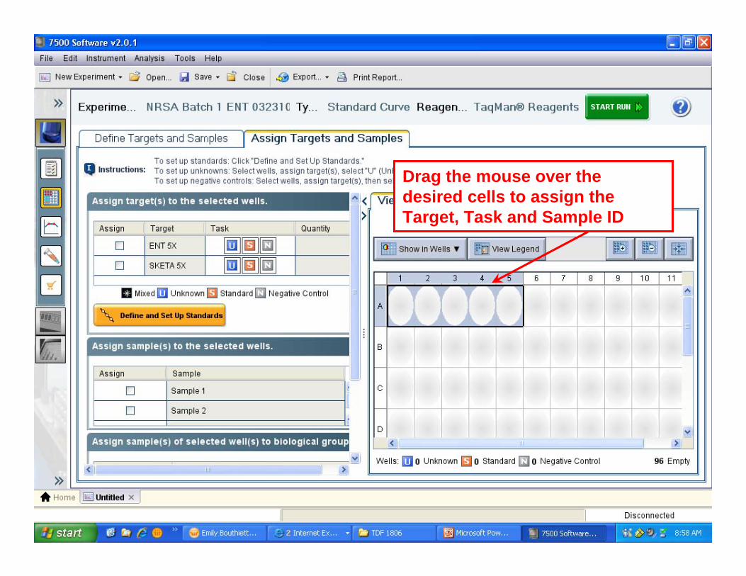

Analysis Menu- Amplification Plot
1 If the plot requires the display of the threshold and baseline select by checking the ldquoUSErdquo boxes in ldquoShowrdquo next to Threshold and Baseline
2 Select ldquoView Well Tablerdquo to view the results in a tabular format
3 Scroll down or sideways for more samples and analysis parameters
Analysis Menu- Standard Curve
Select ldquoStandard Curverdquo to view the results of the samples (if same target) and standards in the plot
Analysis Menu ndash Standard Curve
Standard curve parameters may be useful in data analysis
Click here to select a different Target (if the standards were analyzed in more than one target) or change the Plot Color
Analysis Menu ndash Multicomponent Plot
Select ldquoMulticomponent Plotrdquo to view the variation in the fluorescence of the wells targets or dyes used over the ascending repeat of the 45 thermo cycles
Click on the ldquoPlot Colorrdquo drop down menu to select the parameter based on which the graph required to be plotted
Analysis Menu ndash Raw Data Plot
Select ldquoRaw Data Plotrdquo to view the variation in the emission of fluorescence of the dyes in different filters present over the ascending repeat of the 45 thermo cycles
Drag the pointer on the cycle scale to the desired cycle number to view the variation in the fluorescence through filters of the samples at that cycle
Analysis Menu ndash QC Summary
Select ldquoQC Summaryrdquo to view the analysis summary of the samples in the experiment
Analysis Menu ndash Multiple Plots View
Select ldquoMultiple Plot Viewrdquo to view all the plots for the samples in one window
Each plot has a drop down menu located on the top to access various parameters required to displayed and also has the toolbar feature with various options of printing saving and other parameters
Analysis ndash To Print a Data Report
Click on ldquoPrint Reportrdquo to make a hard copy of the results with required plots
1 Select the required data and plots to be printed by checking the boxes next to the data and plot types in which results can be printed
2 Click ldquoPrint Reportrdquo to print the required data
Method B
Appendix B Cepheid Smart Cyclerreg Operation
Method B
Appendix B - qPCR analysis on Cepheid Smart Cyclerreg
10 Smart Cyclerreg Operation
11 This protocol is intended to provide only information about critical instrument settings required to perform EPA Method B Further details concerning the operation of the instrument can be obtained from the Smart Cyclerreg Operation Manual Cepheid Part D0190 Rev D
12 Turn on the Smart Cyclerreg then the computer
13 Double-click on the Smart Cyclerreg icon on the computer desktop
14 The following steps for defining a protocol are only required before the initial run of the instrument The protocol that is defined in these steps is used in all subsequent runs of the instrument
141 Click on the Define Protocols icon to go to Define Protocols screen
142 Click on the New Protocol button to open the Protocol Name dialog Enter ldquoEPA Method B for the new protocol name and click OK The protocol stages are defined in the series of boxes at the bottom of the Define Protocol screen Make sure the new protocol is highlighted and begin to choose state settings To define Stage 1 click on its drop-down box to display the menu of stage types then select Hold In the Temp column enter 500 and in Secs column enter 120 leaving the Optics setting as the default Off setting (Note This stage is performed to eliminate potential PCR carryover products in the reactions using the Amp-Erasereg UNG enzyme provided in the TaqManreg Universal PCR Master Mix) Note that the optical reading cannot be programmed during a Hold stage
143 To define Stage 2 click on its drop-down box to display the menu of stage types and again select Hold In the Temp column enter 950 and in Secs column enter 600 Again leave the Optics setting on Off (Note This stage is performed to inactivate the Amp-Erasereg UNG enzyme)
144 To define Stage 3 select 2-Temperature Cycle from its drop down menu For the first step enter 950 in the first row of the Temp column and 15 in the Secs column Optics column Off For the second step enter 600 in the second row of the Temp column 120 in the Secs column and click on the Optics cell to select On from the drop-down menu Note This sets the detection of the fluorescence signal to occur at the end of the second step in each cycle Enter 45 in the Repeat field at the top of the Stage 3 box to specify that it should be repeated for 45 cycles Click the Save Protocol button
145 To display primary curve graphs click Define Graphs Highlight FAM in Graph column Check the box for Automatically add to new runs Under Graph Type choose Optics from the pull down menu Under Channels check the box for Ch 1 (FAM) Under Show check the boxes for Primary Curve Threshold (Vertical) and Threshold (Horizontal) Under Axes check the box for Fluorescence vs Cycle At the bottom of the screen click on Save Graph
15 Click on the Create Run icon to open the Create Run screen For each new run enter a unique name in the Run Name field (Note The software does not allow duplicate run names)
16 Enter any additional information about the run in the Notes field Click the arrow in the Dye Set box to display a drop-down menu of the possible selections Select FTTC25 (Note This selects the dye set FAM TET Tex Red Cy5 and a 25 μL reaction)
B-1
Method B
17 Click the AddRemove Sites button The Select Protocols and Sites dialog will appear Highlight (click on) the ldquoEPA Method B protocol developed prior to the first run (Section 142) in the Protocols list In the Sites list highlight the sites on the instrument to be used with this protocol in the current run by clicking on them with the shift key held down (Note Sites refer to the I-core modules in the Smart Cyclerreg processing block in which reaction tubes will be placed a total of 16 are possible per block When using multiple blocks the site numbers will be preceded by the block letters eg A B C) then click the right pointing arrow to transfer the selected sites and protocol to the Selections table
18 Click on the OK button to save the selections and return to the Create Run screen
19 Place the loaded Smart Cyclerreg reaction tubes in the I-core module slots selected above for current run The tubes should snap into place Either the front or back of the caps can face the front of the processing block
110 In one of the View menus that is shown select Analysis Settings The displayed table includes one row for each of the four possible dye channels defined in the dye set Click on the cell in the FAM row under the Usage column heading and select Assay from the drop down menu Set the Usage cells for all other dyes to Unused in the same manner (Note All assays in this protocol use FAM as the reporter dye) All other cells in this table should be left at default settings (See Smart Cyclerreg Operation Manual)
111 In the other View menu that is shown select the Results Table Enter the sample identification information for each site in the Sample ID column (additional information can be entered into the Notes column) Leave the other columns as default settings (see Smart Cyclerreg Operation Manual)
112 Click on the Start Run button The orange LEDs on the Smart Cyclerreg processing block should turn on and the software will automatically switch to the View Results screen
113 To display the real time temperature profiles for all sites click Temperature in either of the View menus To display real time growth curves for all samples (ie the fluorescence signal vs cycle) click FAM in the other View menu
114 At the end of the run it is recommended to check the cycle threshold values calculated by the instrument for each sample by opening the Results Table window by clicking on this selection in the upper View menu It is also recommended to inspect the growth curves in the FAM window which can be opened in the same manner from the lower View menu The default threshold fluorescence value is shown in this window as a single horizontal red line and the cycle thresholds for each site are shown as vertical red lines To view the data for individual sites in this window click on that site number in the table to the right of the graph If the default threshold fluorescence line is well above all of the growth curve lines prior to visible amplification the threshold fluorescence value can be changed to a lower value This is done by reopening the Analysis Settings window from the upper View menu and entering a new value in the Manual Thresh Fluor Units cell in the FAM row Conversely if the default threshold fluorescence line is below any of the growth curve lines prior to visible amplification the threshold fluorescence value should be changed to a higher value in the same manner Previous studies have indicated that a threshold value of 8 works well for most analyses Click on the Update Analysis button to view the new threshold line in the FAM window The cycle threshold values will be automatically updated in the Results Table
115 Once the threshold fluorescence value is adjusted to an optimal value click the Save Run button (Note The Smart Cyclerreg Software does not give a prompt to save changes before printing or exporting Therefore it is possible to make changes to the Results Table or Analysis Settings and immediately print or export the data then close the run without saving the changes In this case
B-2
Method B
the data saved in the Smart Cyclerreg database will not match the printed or exported data If no changes are made in the threshold fluorescence value the run data is automatically saved as it is when the program is closed or a new run is created)
116 To set up automatic export of raw data (see ldquoHow To Set Up Automatic Export of Raw Datardquo for screen shots) from the main menu click on Setup then System Defaults then Export Settings From the Export Settings dialog box check the box beside Results Table and Analysis Settings Click the Browse button to select the folder where you want your raw data saved Click on the radio button next to Automatic export on run completion then click the OK button
117 To manually save the Results Table and Analysis setting containing the instrument-calculated cycle threshold values for each sample (see ldquoHow to Manually Export Raw Datardquo for screen shots) click the Export button to display the Export Data dialog box Check the box next to the heading Export Results Table and Analysis Settings by clicking on it Leave all other boxes unchecked Click on Export A box labeled Export Data will appear with the run name in the file name box Click on the drop down menu to the right of Save In at the top left of the screen to change the directory where you want your data saved Always save to the hard drive Click on Save Data are exported as comma-delimited text (cvs) files in MS Excel-compatible files to the Export folder in the Smart Cyclerreg folder CSmart CyclerregExport Analysts will late save the file as an XLS file
118 To archive a run in the Smart Cyclerreg program click on Tools From the drop down menu click on Data Management and then Archive Runs Click Proceed Select the run to be archived by clicking on its name in the database list Click OK and then Proceed A box labeled Archive Run will appear on the screen There will be a line labeled Save in Input which directory you would like the run to be saved in There will be a line File Name Enter a file name Click Save Click OK
119 To print run data (see ldquoHow to Print Run Datardquo for screen shots) after the run is completed right click on the graph area and select Print then Print Graph with Results Table An Optics Graph print preview screen will pop up click Print The screen will switch back to the post run screen To print the generated report click Report A Run Report print preview screen will pop up click Print
120 To set up a new analysis (see ldquoHow to Set Up a New Runrdquo for screen shots) from the post run screen click Create Run at the top left The results of your just completed will disappear and an AddRemove Sites button will appear in the middle of the screen ndash click it A Select Protocols and Sites screen will pop up select EPA Method B in the Protocols box and highlight the amount of sites needed for the assay (A1-A16) in the Sites box Click the right arrow to the right of the sites box to move the sights to the Selections box After double checking that the correct protocol is highlighted click OK Add the Run Name in the Run Name box The Site ID Protocol Sample ID Sample Type Notes (etc) box will pop up Enter the Sample ID for each site Under this box find the Usage column and click on Assay to select Unused for Cy3 TxR and Cy5 (leave Assay for FAM) In the same box find the Manual Thresh Fluor Units and click on the units for FAM to change it from 300 to 80 (leave the units at 300 for Cy3 TxR and Cy5) After loading the Smart Cycler with tubes click Start Run A red light should appear on sites that are in use
B-3
How to Set Up a New Experiment Using the Smart Cyclerreg (Software Version 20)
1 Click on ldquoNew Protocolrdquo
2 This screen will appear - type in the name of the new protocol
3 Click on OK when done
1 New Protocol name will appear in list Make sure new protocol is highlighted and begin to choose stage settings
2 Set the Temperature in the ldquoHOLDrdquo stage to 500 degrees and 120 seconds NOTE optical readings cannot be programmed during a HOLD stage
In Stage 2 set the temperature to 950 degrees and 600 seconds
1 In Stage 3 set the drop down menu at ldquo2-Temperature Cyclerdquo to repeat 45 times (cycles)
2 For the first temp cycle set the temp at 95 degrees for 15 seconds with optics OFF
3 In the second Temp cycle set the temp for 60 degrees for 120 seconds with the optics ON
4 Click Save Protocol when finished
How To Set Up Automatic Export of Raw Data
To set up automatic export of Raw Data into computer click on ldquoSETUPrdquo then ldquoSystem Defaultsrdquo then ldquoExport Settingsrdquo
1 Check Results Table and Analysis settings box
3 Be sure that Automatic export on run completion is checked
2 Choose browse to select a folder where the raw data will export to
4 Click OK when finished
How To Manually Export Raw Data
Once run is finished click Export
Check the Export Results Table and Analysis Settings box then click ldquoExportrdquo
Choose the appropriate file folder to save the Raw Data to and click SAVE NOTE All raw data will export in the form of a CSV file Analysts will later save file as an ldquoXLSrdquo file
How to Print Run Data
Right click on graph area and select ldquoPrintrdquo then ldquoPrint Graph with Results Tablerdquo
This sheet will pop up Click ldquoPrintrdquo to print file
To print the generated report click on ldquoReportrdquo
Click ldquoPrintrdquo to print out the generated run data report
How to Set Up a New Run
Click ldquoCreate Runrdquo
Click ldquoAddRemoverdquo Sites
1 Be sure the correct protocol is highlighted before selecting sites
2 Highlight the amount of sites needed for assay (A1-A16)
Click ldquorightrdquo arrow to move sites to the ldquoSelectionsrdquo column
Sites have been moved to selections column Double check that the correct protocol is selected and click on ldquoOKrdquo
The Sample IDs and run name can be entered at this point
Under the ldquoUsagerdquo column select ldquoUnusedrdquo from the drop down menu for Cy3 TxR and Cy5 Leave the ldquoAssayrdquo on the FAM line for this particular protocol
1 Set the Manual Threshold Fluorescence Units to 80 on the FAM line
2 When smart cycler tubes have been put in to appropriate sites click ldquoStart Runrdquo - a red light should appear on sites that are in use

Method B
the data saved in the Smart Cyclerreg database will not match the printed or exported data If no changes are made in the threshold fluorescence value the run data is automatically saved as it is when the program is closed or a new run is created)
116 To set up automatic export of raw data (see ldquoHow To Set Up Automatic Export of Raw Datardquo for screen shots) from the main menu click on Setup then System Defaults then Export Settings From the Export Settings dialog box check the box beside Results Table and Analysis Settings Click the Browse button to select the folder where you want your raw data saved Click on the radio button next to Automatic export on run completion then click the OK button
117 To manually save the Results Table and Analysis setting containing the instrument-calculated cycle threshold values for each sample (see ldquoHow to Manually Export Raw Datardquo for screen shots) click the Export button to display the Export Data dialog box Check the box next to the heading Export Results Table and Analysis Settings by clicking on it Leave all other boxes unchecked Click on Export A box labeled Export Data will appear with the run name in the file name box Click on the drop down menu to the right of Save In at the top left of the screen to change the directory where you want your data saved Always save to the hard drive Click on Save Data are exported as comma-delimited text (cvs) files in MS Excel-compatible files to the Export folder in the Smart Cyclerreg folder CSmart CyclerregExport Analysts will late save the file as an XLS file
118 To archive a run in the Smart Cyclerreg program click on Tools From the drop down menu click on Data Management and then Archive Runs Click Proceed Select the run to be archived by clicking on its name in the database list Click OK and then Proceed A box labeled Archive Run will appear on the screen There will be a line labeled Save in Input which directory you would like the run to be saved in There will be a line File Name Enter a file name Click Save Click OK
119 To print run data (see ldquoHow to Print Run Datardquo for screen shots) after the run is completed right click on the graph area and select Print then Print Graph with Results Table An Optics Graph print preview screen will pop up click Print The screen will switch back to the post run screen To print the generated report click Report A Run Report print preview screen will pop up click Print
120 To set up a new analysis (see ldquoHow to Set Up a New Runrdquo for screen shots) from the post run screen click Create Run at the top left The results of your just completed will disappear and an AddRemove Sites button will appear in the middle of the screen ndash click it A Select Protocols and Sites screen will pop up select EPA Method B in the Protocols box and highlight the amount of sites needed for the assay (A1-A16) in the Sites box Click the right arrow to the right of the sites box to move the sights to the Selections box After double checking that the correct protocol is highlighted click OK Add the Run Name in the Run Name box The Site ID Protocol Sample ID Sample Type Notes (etc) box will pop up Enter the Sample ID for each site Under this box find the Usage column and click on Assay to select Unused for Cy3 TxR and Cy5 (leave Assay for FAM) In the same box find the Manual Thresh Fluor Units and click on the units for FAM to change it from 300 to 80 (leave the units at 300 for Cy3 TxR and Cy5) After loading the Smart Cycler with tubes click Start Run A red light should appear on sites that are in use
B-3
How to Set Up a New Experiment Using the Smart Cyclerreg (Software Version 20)
1 Click on ldquoNew Protocolrdquo
2 This screen will appear - type in the name of the new protocol
3 Click on OK when done
1 New Protocol name will appear in list Make sure new protocol is highlighted and begin to choose stage settings
2 Set the Temperature in the ldquoHOLDrdquo stage to 500 degrees and 120 seconds NOTE optical readings cannot be programmed during a HOLD stage
In Stage 2 set the temperature to 950 degrees and 600 seconds
1 In Stage 3 set the drop down menu at ldquo2-Temperature Cyclerdquo to repeat 45 times (cycles)
2 For the first temp cycle set the temp at 95 degrees for 15 seconds with optics OFF
3 In the second Temp cycle set the temp for 60 degrees for 120 seconds with the optics ON
4 Click Save Protocol when finished
How To Set Up Automatic Export of Raw Data
To set up automatic export of Raw Data into computer click on ldquoSETUPrdquo then ldquoSystem Defaultsrdquo then ldquoExport Settingsrdquo
1 Check Results Table and Analysis settings box
3 Be sure that Automatic export on run completion is checked
2 Choose browse to select a folder where the raw data will export to
4 Click OK when finished
How To Manually Export Raw Data
Once run is finished click Export
Check the Export Results Table and Analysis Settings box then click ldquoExportrdquo
Choose the appropriate file folder to save the Raw Data to and click SAVE NOTE All raw data will export in the form of a CSV file Analysts will later save file as an ldquoXLSrdquo file
How to Print Run Data
Right click on graph area and select ldquoPrintrdquo then ldquoPrint Graph with Results Tablerdquo
This sheet will pop up Click ldquoPrintrdquo to print file
To print the generated report click on ldquoReportrdquo
Click ldquoPrintrdquo to print out the generated run data report
How to Set Up a New Run
Click ldquoCreate Runrdquo
Click ldquoAddRemoverdquo Sites
1 Be sure the correct protocol is highlighted before selecting sites
2 Highlight the amount of sites needed for assay (A1-A16)
Click ldquorightrdquo arrow to move sites to the ldquoSelectionsrdquo column
Sites have been moved to selections column Double check that the correct protocol is selected and click on ldquoOKrdquo
The Sample IDs and run name can be entered at this point
Under the ldquoUsagerdquo column select ldquoUnusedrdquo from the drop down menu for Cy3 TxR and Cy5 Leave the ldquoAssayrdquo on the FAM line for this particular protocol
1 Set the Manual Threshold Fluorescence Units to 80 on the FAM line
2 When smart cycler tubes have been put in to appropriate sites click ldquoStart Runrdquo - a red light should appear on sites that are in use

1 Set the Manual Threshold Fluorescence Units to 80 on the FAM line
2 When smart cycler tubes have been put in to appropriate sites click ldquoStart Runrdquo - a red light should appear on sites that are in use