Method for Bias Field Correction of Brain T1-Weighted Magnetic

Method for Bias Field Correction of BrainT1-Weighted Magnetic Resonance Images

Minimizing Segmentation Error

Juan D. Gispert, Santiago Reig, Javier Pascau, Juan J. Vaquero,Pedro Garcıa-Barreno, and Manuel Desco*

Laboratorio de Imagen Medica, Medicina y Cirugıa Experimental, Hospital General Universitario“Gregorio Maranon,” Madrid, Spain

� �

Abstract: This work presents a new algorithm (nonuniform intensity correction; NIC) for correction ofintensity inhomogeneities in T1-weighted magnetic resonance (MR) images. The bias field and a bias-freeimage are obtained through an iterative process that uses brain tissue segmentation. The algorithm wasvalidated by means of realistic phantom images and a set of 24 real images. The first evaluation phase wasbased on a public domain phantom dataset, used previously to assess bias field correction algorithms. NICperformed similar to previously described methods in removing the bias field from phantom images,without introduction of degradation in the absence of intensity inhomogeneity. The real image datasetwas used to compare the performance of this new algorithm to that of other widely used methods (N3,SPM’99, and SPM2). This dataset included both low and high bias field images from two different MRscanners of low (0.5 T) and medium (1.5 T) static fields. Using standard quality criteria for determiningthe goodness of the different methods, NIC achieved the best results, correcting the images of the real MRdataset, enabling its systematic use in images from both low and medium static field MR scanners. Alimitation of our method is that it might fail if the bias field is so high that the initial histogram does notshow bimodal distribution for white and gray matter. Hum. Brain Mapp. 22:133–144, 2004.© 2004 Wiley-Liss, Inc.

Key words: nonuniform intensity correction; NIC; magnetic resonance imaging; bias field; intensityinhomogeneities; segmentation algorithms

� �

INTRODUCTION

Segmentation of magnetic resonance (MR) images is afundamental procedure for the quantitative study of differ-ent brain pathologies such as multiple sclerosis [Miller et al.,2002], Alzheimer’s disease [Good et al., 2002], or schizophre-nia [Lawrie and Abukmeil, 1998; Weinberger and McClure,2002]. Automatic segmentation of MR scans is very usefulfor these applications, although it may be hindered by sev-eral acquisition-related artifacts.

One such artifact is the lack of homogeneity of the radio-frequency (RF) or B1 field, also known as “illuminationartifact” or “bias field,” which consists of a smooth multi-plicative variation of intensity levels across the MR image. Ina standard 1.5 T MR scanner, the magnitude of this intensityvariation may even exceed 30% of the signal value [Guil-

Contract grant sponsor: Communidad de Madrid; Contract grantnumber: III-PRICIT; Contract grant sponsor: FIS, Ministerio deSanidad; Contract grant numbers: Red Timatica IM3, PI-021178;Contract grant sponsor: Ministeri de Ciencia y Tecnologia; Contractgrant number: TIC-2001-3697-C03.*Correspondence to: Dr. Manuel Desco, Medicina y Cirugıa Exper-imental, Hospital General Universitario “Gregorio Maranon,” Dr.Esquerdo, 46 Madrid, E-28007 Spain. E-mail: [email protected] for publication 17 April 2003; Accepted 1 December 2003DOI 10.1002/hbm.20013

� Human Brain Mapping 22:133–144(2004) �

© 2004 Wiley-Liss, Inc.

lemaud and Brady, 1997]. Although this artifact may beunnoticeable to the eye, it can clearly degrade the volumetricquantification of cerebral tissues, particularly when usingautomatic segmentation algorithms based on intensity lev-els. For this reason, bias field correction algorithms are usedmainly to reduce classification error rates (CER) when seg-menting images into different tissue types.

This artifact may have several causes, such as lack ofuniform sensitivity of the RF emitting and receiving coils,static field (B0) inhomogeneities, gradient-induced eddy cur-rents, magnetic susceptibility of tissue, interslice cross-talk,RF standing wave effects, and attenuation of the RF signalinside the object [Simmons et al., 1994; Sled and Pike, 1998].Magnitude of the bias field is stronger in high static fieldmachines because of the higher RF frequencies used. Acorrective calibration, as is usually carried out with mag-netic field inhomogeneity [Cusack et al., 2003], is not feasiblebecause the attenuation depends on every individual sampleand precludes any static correction. Some methods devel-oped for the measurement of the RF inhomogeneity in vivoare not practical for the clinical routine, as they requirespecific equipment and are time consuming [Sled and Pike,1998]. Correction of the bias field therefore is addressedusually by post-acquisition mathematical algorithms.

The different correction strategies proposed can be classi-fied roughly into two types, depending on whether they usesegmentation or not. Many examples can be found of differ-ent algorithms for correcting intensity inhomogeneities thatdo not use any segmentation. Homomorphic filtering meth-ods [Brinkmann et al., 1998; Johnston et al., 1996] assumedno overlapping between the low-frequency bias field andthe high-frequency image information. Dawant et al. [1993]proposed a method to correct image intensities based on aprevious selection (either manual or automatic) of referencepoints in white matter. The method in DeCarli et al. [1996]was based on differences between local and global medians.Vokurka et al. [1999] combined two methods to correct intra-and interslice intensity nonuniformity, whose effect on sur-face coil images was studied further [Vokurka et al., 2001].Cohen et al. [2000] applied a gaussian filtering scheme,minimizing filtering artifacts by assigning the mean signalintensity to the background voxels. The methods by Mangin[2000] and Likar et al. [2001] fitted the bias field with para-metric basis functions whose coefficients were determinedthrough entropy minimization. Another approach has beento take the intensity inhomogeneity artifact into accountduring the MR reconstruction process [Schomberg, 1999].

All these methods do not make use of any tissue segmen-tation; however, the bias field correction can be improvednoticeably by taking advantage of a tissue classification.Following this strategy, different methods have been devel-oped that simultaneously carry out the tissue segmentationand the field correction. An iterative method based on theexpectation-maximization (EM) algorithm was proposed byWells et al. [1996] and improved by Guillemaud and Brady[1997]. All these methods involve the following steps: (1)classification of the image voxels into a set of predefined

tissue classes; (2) calculation of a bias-free image by assign-ing voxels in each class its mean tissue intensity; (3) calcu-lation of a residual image as the subtraction of the bias-freeimage from the original image; (4) estimation of the biasfield by smoothing the residual image; and (5) correction ofthe original image using this estimated bias field. The wholeprocess is iterated until no improvement is observed in acertain quality parameter.

The method in Ashburner and Friston [1997] introducedprior spatial information into the classification step by mak-ing use of a probabilistic template. This method, detailedfurther by Ashburner and Friston [2000], was included in theSPM99 software package, and a newer version of the algo-rithm (SPM2) has been released recently [Ashburner, 2002].Van Leemput et al. [1999a,b] modified the algorithm byadding a Markov model to steer the tissue classification.Several other methods have adopted similar strategies: TheN3 algorithm [nonparametric nonuniform intensity normal-ization; Sled et al., 1998] used an iterative algorithm toestimate both the multiplicative bias field (represented by acombination of smooth B-splines) and the distribution of thetrue tissue intensities in the MR volume. Shattuck et al.[2001] followed an analogous scheme, also fitting B-splinesto local estimates of the bias field. Pham and Prince [1999]and Ahmed et al. [2002] estimated the bias field using anadaptive fuzzy C-means classification together with a mul-tiscale pyramidal algorithm. Zhang et al. [2001] made use ofa hidden Markov model to simultaneously carry out thesegmentation and the correction. Marroquin et al. [2002]modeled separately the intensity inhomogeneity of each tis-sue class using parametric models.

The lack of an optimal solution is thus highlighted bymany bias field correction strategies in the literature. Unfor-tunately, evaluation and testing of all these algorithms havenot received the same attention. Velthuizen et al. [1998]carried out a review of MRI intensity nonuniformity correc-tion methods and an evaluation of their impact on measure-ments of brain tumor volumes. They reported that tumorsegmentation was not improved by these methods, and theresult was attributed to the fact that tumors are usually verylocalized. Another comprehensive article by Arnold et al.[2001] showed a quantitative comparison of the six mostrepresentative algorithms used currently to correct inhomo-geneity artifacts. Their main conclusion was that none of themethods performed ideally in all cases, particularly consid-ering that some methods were not robust with images show-ing little or no bias field effect. Locally adaptive methodsprovided more accurate corrections than did non-adaptivetechniques, suggesting that the former are more efficientwhen dealing with some features of brain anatomical vari-ability, like the asymmetry between left and right hemi-spheres. Chard et al. [2002] investigated the reproducibilityof the SPM99 segmentation method for the assessment ofbrain volume measurements and concluded that the biasfield correction markedly improved the repeatability of tis-sue segmentation.

� Gispert et al. �

� 134 �

Despite its unquestionable interest, the use of real imagedatasets to measure the efficiency and robustness of theinhomogeneity correction raises the problem of establishingappropriate goodness criteria. The use of phantom imagessimplifies evaluation of correction algorithms, because a biasfield of known magnitude can be added easily. When mea-suring the efficiency of correction algorithms with real im-age datasets, the actual bias field in the images is not known.

Our work presents a new, locally adaptive algorithm forcorrection of the bias field artifact in T1-weighted MR scansbased on minimization of the CER between different cere-bral tissues. The algorithm has been validated with an avail-able realistic phantom, used previously in the study byArnold et al. [2001]. Our results were compared to thosereported in that work. In addition, the usefulness of ouralgorithm for segmentation has been evaluated on real im-ages obtained by scanning a set of subjects in two MRmachines of low (0.5 T) and medium (1.5 T) field. Thealgorithm was compared to three of the most widely usedcorrection methods (N3 [Sled et al., 1998], SPM99 [Ash-burner and Friston, 2000], and SPM2 [Ashburner, 2002]),using commonly accepted criteria.

MATERIAL AND METHODS

The rationale of our algorithm (NIC; nonuniform intensitycorrection) is to make use of the estimated error rate of atissue segmentation as a goodness parameter for correctionof the bias field. The algorithm estimates a CER by modelingtissue intensities with a mixture of basis functions and mea-suring their overlap.

Description of the NIC Algorithm

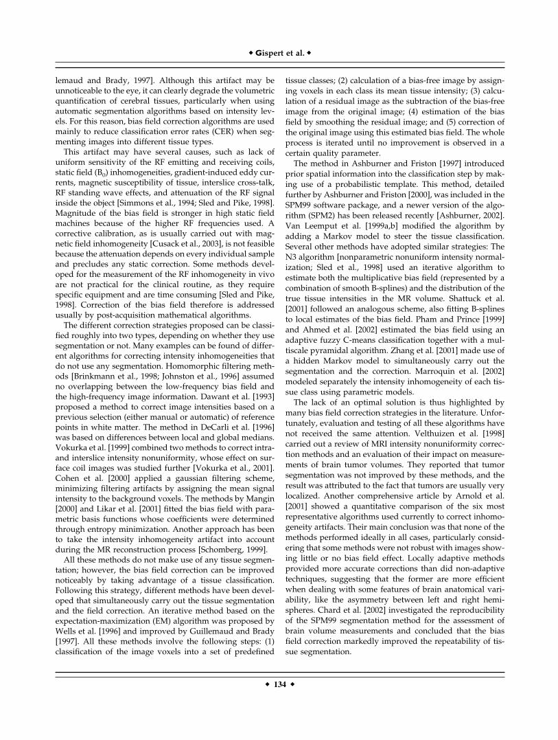
The NIC algorithm iterates two major stages, “tissue clas-sification” and “bias field estimation.” The tissue classifica-tion stage provides information to create a bias-free image,used in the second stage to obtain both an estimation of theinhomogeneity field in the original image and a CER. Be-cause the bias field is assumed to be smooth and multipli-cative, it can be estimated as the quotient between smoothedversions of the original and bias-free images. The algorithmiterates until no improvement of the CER is achieved inthree successive steps. Figure 1 shows a flowchart of thewhole process.

Tissue Classification

For the algorithm to operate properly, no more than threetissues types must appear: gray matter, white matter, andcerebrospinal fluid (CSF). This makes it necessary to excludeall the extracranial voxels using a segmentation method. Inour case, this segmentation, available previously, had beenobtained by thresholding the original image and manuallyediting the extracranial mask obtained. This task is not crit-ical, however, and could be accomplished using any of themany different automatic methods available [Atkins andMackiewich, 1998; Brummer et al., 1993; Shattuck et al., 2001;Stokking et al., 2000]. The histogram of the masked image is

modeled with five basis functions: three gaussians corre-sponding to pure cerebral tissues (white and gray matterand CSF) and two additional probability densities for partialvolume voxels, assumed to contain only two pure tissues(gray–white matter and CSF–gray matter). Different statis-tical models for partial volume voxels are thoroughly de-scribed in Santago and Gage [1995]. Following the notationof Ruan et al. [2000], the partial volume density functions aredefined by

p(ym) � �0

1

p(ym,a) da (1)

where

p(ym,a) �1

�2��a2�12 � (1 � a)2�2

2 �

exp��[ym � (a�1 � �1 � a)�2)]2

2[a2�12 � (1 � a)2�2

2] � (2)

Figure 1.Flowchart of the NIC algorithm.

� Bias Field Correction of T1-Weighted MR Images �

� 135 �

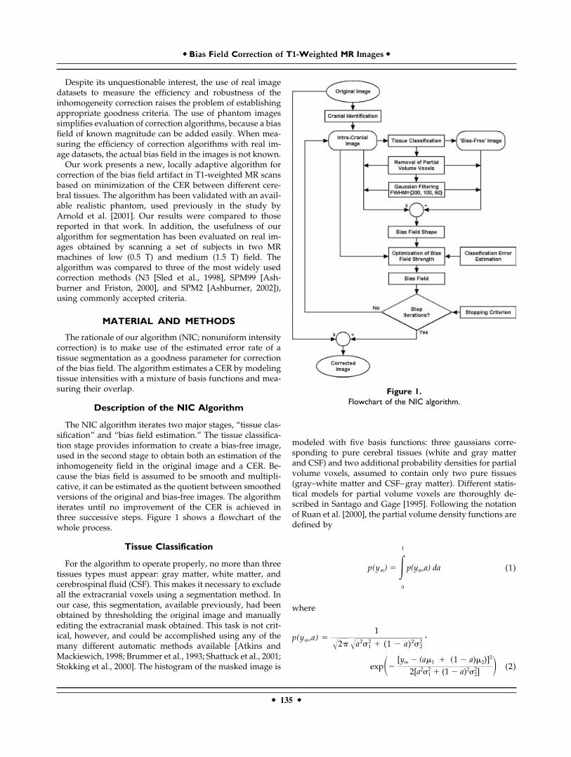
being p(ym, a) the probability of a voxel with proportions ofpure tissues a and (1 � a) to present an intensity level ym.Mean and standard deviation of the intensity levels of thepure tissues are represented by (�1, �2) and (�1, �2) respec-tively (Fig. 2a). This model assumes that all a values occurwith the same probability, because partial volume voxelsmay consist of any fraction of pure tissue classes. Parametersof the basis functions are estimated iteratively with an EM(expectation-maximization) algorithm [Dempster et al.,1977]. At each EM iteration, a Bayesian approach is used tocalculate the classification thresholds that yield the mini-mum error rate. This error rate is estimated as the overlapbetween pure tissue distributions (Fig. 2b). The EM algo-rithm stops when the segmentation thresholds do notchange in 10 consecutive iterations. The result of this stage isan estimation of the parameters of basis functions thatmodel the image histogram.

Bias Field Estimation

In this stage, the parameters of the basis functionsprovided by the tissue classification are used to create abias-free image. Those intracranial voxels with an inten-sity level within the 95% confidence intervals (95% CI) ofany of the two partial volume basis functions are classi-fied as partial volume. The remaining intracranial voxelsare considered pure tissue and classified into gray matter,white matter, and CSF using the minimum error-rateclassification thresholds obtained in the tissue classifica-tion stage. The value of these pure tissue voxels ischanged to the mean intensity of their correspondingtissue class (Fig. 3b), thus producing a bias-free image.Following the strategy proposed by Cohen et al. [2000] toreduce filtering artifacts, the values of all extracranial andpartial volume voxels are set to the mean intracranial

Figure 2.a: Example of a theoretical density distributionfor the partial volume voxels according to themodel implemented in the NIC algorithm.Probability density functions of two tissuetypes and of their partial volume voxels areshown (Tissue 1 mean � 200 � 50; Tissue 2mean � 800 � 100). b: Example of real MRhistogram fitted by five basis functions. Puretissue and partial volume voxel basis functionsare highlighted. The segmentation error canbe estimated as the overlap between the basisfunctions.


� 136 �

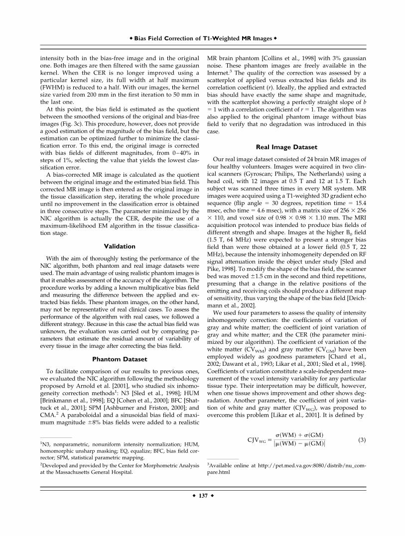
intensity both in the bias-free image and in the originalone. Both images are then filtered with the same gaussiankernel. When the CER is no longer improved using aparticular kernel size, its full width at half maximum(FWHM) is reduced to a half. With our images, the kernelsize varied from 200 mm in the first iteration to 50 mm inthe last one.

At this point, the bias field is estimated as the quotientbetween the smoothed versions of the original and bias-freeimages (Fig. 3c). This procedure, however, does not providea good estimation of the magnitude of the bias field, but theestimation can be optimized further to minimize the classi-fication error. To this end, the original image is correctedwith bias fields of different magnitudes, from 0–40% insteps of 1%, selecting the value that yields the lowest clas-sification error.

A bias-corrected MR image is calculated as the quotientbetween the original image and the estimated bias field. Thiscorrected MR image is then entered as the original image inthe tissue classification step, iterating the whole procedureuntil no improvement in the classification error is obtainedin three consecutive steps. The parameter minimized by theNIC algorithm is actually the CER, despite the use of amaximum-likelihood EM algorithm in the tissue classifica-tion stage.

Validation

With the aim of thoroughly testing the performance of theNIC algorithm, both phantom and real image datasets wereused. The main advantage of using realistic phantom images isthat it enables assessment of the accuracy of the algorithm. Theprocedure works by adding a known multiplicative bias fieldand measuring the difference between the applied and ex-tracted bias fields. These phantom images, on the other hand,may not be representative of real clinical cases. To assess theperformance of the algorithm with real cases, we followed adifferent strategy. Because in this case the actual bias field wasunknown, the evaluation was carried out by comparing pa-rameters that estimate the residual amount of variability ofevery tissue in the image after correcting the bias field.

Phantom Dataset

To facilitate comparison of our results to previous ones,we evaluated the NIC algorithm following the methodologyproposed by Arnold et al. [2001], who studied six inhomo-geneity correction methods1: N3 [Sled et al., 1998]; HUM[Brinkmann et al., 1998]; EQ [Cohen et al., 2000]; BFC [Shat-tuck et al., 2001]; SPM [Ashburner and Friston, 2000]; andCMA.2 A paraboloidal and a sinusoidal bias field of maxi-mum magnitude �8% bias fields were added to a realistic

MR brain phantom [Collins et al., 1998] with 3% gaussiannoise. These phantom images are freely available in theInternet.3 The quality of the correction was assessed by ascatterplot of applied versus extracted bias fields and itscorrelation coefficient (r). Ideally, the applied and extractedbias should have exactly the same shape and magnitude,with the scatterplot showing a perfectly straight slope of b� 1 with a correlation coefficient of r � 1. The algorithm wasalso applied to the original phantom image without biasfield to verify that no degradation was introduced in thiscase.

Real Image Dataset

Our real image dataset consisted of 24 brain MR images offour healthy volunteers. Images were acquired in two clin-ical scanners (Gyroscan; Philips, The Netherlands) using ahead coil, with 12 images at 0.5 T and 12 at 1.5 T. Eachsubject was scanned three times in every MR system. MRimages were acquired using a T1-weighted 3D gradient echosequence (flip angle � 30 degrees, repetition time � 15.4msec, echo time � 4.6 msec), with a matrix size of 256 256 110, and voxel size of 0.98 0.98 1.10 mm. The MRIacquisition protocol was intended to produce bias fields ofdifferent strength and shape. Images at the higher B0 field(1.5 T, 64 MHz) were expected to present a stronger biasfield than were those obtained at a lower field (0.5 T, 22MHz), because the intensity inhomogeneity depended on RFsignal attenuation inside the object under study [Sled andPike, 1998]. To modify the shape of the bias field, the scannerbed was moved �1.5 cm in the second and third repetitions,presuming that a change in the relative positions of theemitting and receiving coils should produce a different mapof sensitivity, thus varying the shape of the bias field [Deich-mann et al., 2002].

We used four parameters to assess the quality of intensityinhomogeneity correction: the coefficients of variation ofgray and white matter; the coefficient of joint variation ofgray and white matter; and the CER (the parameter mini-mized by our algorithm). The coefficient of variation of thewhite matter (CVWM) and gray matter (CVGM) have beenemployed widely as goodness parameters [Chard et al.,2002; Dawant et al., 1993; Likar et al., 2001; Sled et al., 1998].Coefficients of variation constitute a scale-independent mea-surement of the voxel intensity variability for any particulartissue type. Their interpretation may be difficult, however,when one tissue shows improvement and other shows deg-radation. Another parameter, the coefficient of joint varia-tion of white and gray matter (CJVWG), was proposed toovercome this problem [Likar et al., 2001]. It is defined by

CJVWG ��WM � ��GM

��WM � ��GM� (3)1N3, nonparametric, nonuniform intensity normalization; HUM,homomorphic unsharp masking; EQ, equalize; BFC, bias field cor-rector; SPM, statistical parametric mapping.2Developed and provided by the Center for Morphometric Analysisat the Massachusetts General Hospital.

3Available online at http://pet.med.va.gov:8080/distrib/nu_com-pare.html


� 137 �

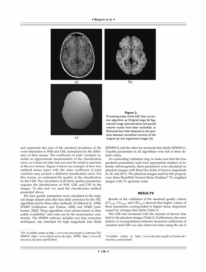
and represents the sum of the standard deviations of thevoxel intensities in WM and GM, normalized by the differ-ence of their means. The coefficient of joint variation re-mains an approximate measurement of the classificationerror, as it does not take into account the relative amountsof the two tissues. Figure 4 shows an example of how twoartificial tissue types with the same coefficient of jointvariation may present a different classification error. Forthis reason, we estimated the quality of the classificationby the CER. The calculation of all these quality parametersrequires the identification of WM, GM, and CSF in theimages. To this end, we used the classification methodpresented above.

The four quality parameters were calculated in the origi-nal image dataset and after bias field correction by the NICalgorithm and by three other methods: N3 [Sled et al., 1998],SPM99 [Ashburner and Friston, 2000] and SPM2 [Ash-burner, 2002]. These algorithms were chosen based on theirpublic availability4 and wide use by the neuroscience com-munity. The SPM99 software includes two bias correctiontechniques, one intended for high magnitude bias fields

(SPM99-S) and the other for moderate bias fields (SPM99-L).Tunable parameters in all algorithms were left at their de-fault values.

As a preceding validation step, to make sure that the fourgoodness parameters used were appropriate markers of in-tensity inhomogeneity, these parameters were calculated onphantom images with three bias fields of known magnitude(0, 20, and 40%). The phantom images used for this purposewere three BrainWeb Normal Brain Database5 T1-weightedimages with 3% gaussian noise.

RESULTS

Results of the validation of the standard quality criteria(CVGM, CVWM, and CJVWG) showed that higher values ofthese parameters corresponded to higher tissue dispersioncaused by stronger bias fields (Table I).

The CER also increased with the amount of known biasfield in the phantom images (Table I). Furthermore, the samepattern of correspondence between increased coefficients ofvariation and CER was also observed when using the set of

4N3: Available online at http://www.bic.mni.mcgill.ca/software/N3;SPM’99: http://www.fil.ion.ucl.ac.uk/spm; SPM2: http://www.fil.ion.ucl.ac.uk/spm/spm2b.html

5Available online at http://www.bic.mni.mcgill.ca/brainweb/selection_normal.html

Figure 3.Processing steps of the NIC bias correc-tion algorithm. a: Original image. b: Seg-mented image (extracerebral and partialvolume voxels have been excluded). c:Estimated bias field obtained as the quo-tient between smoothed versions of theoriginal (a) and segmented images (b).


� 138 �

real images (Table II). These results support the validity ofusing the CER criterion as a measurement of the amount ofbias field in the images.

Validation of NIC Using Phantom Images

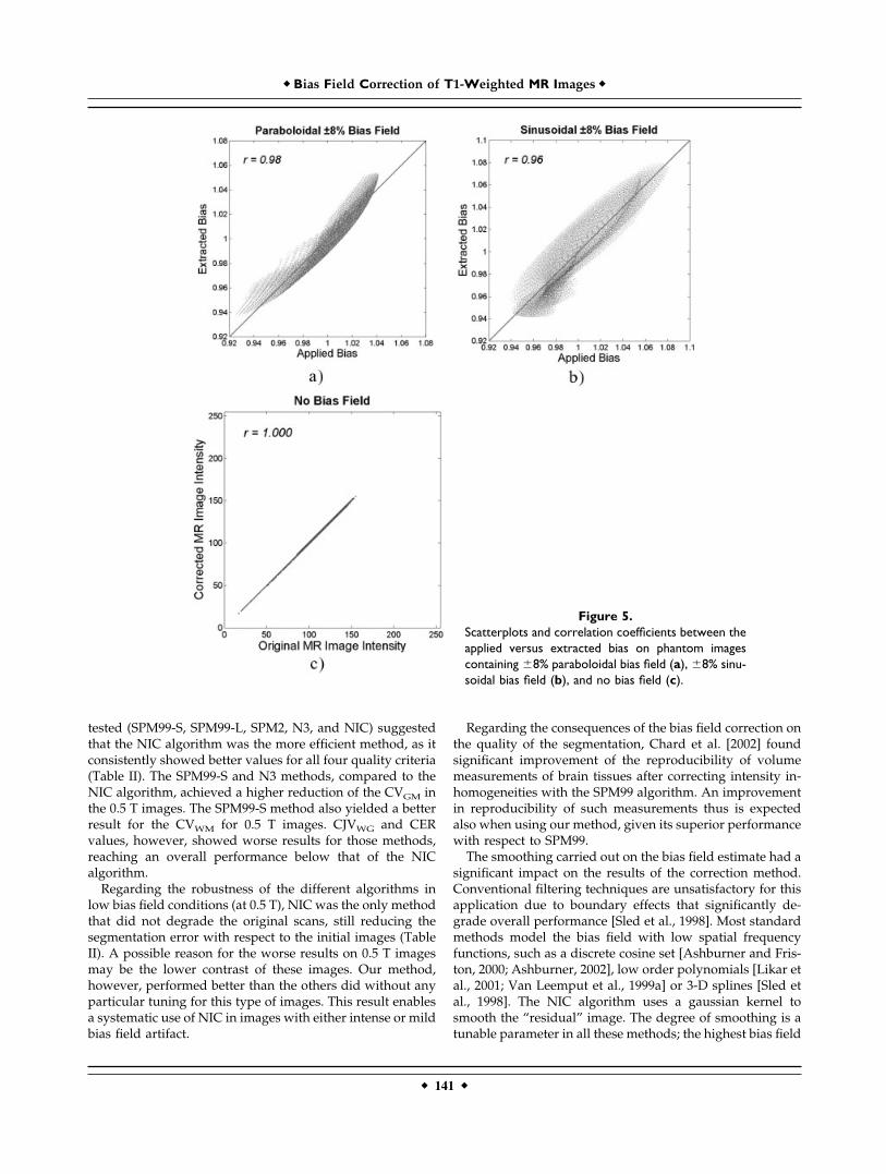
Scatterplots of the applied versus extracted bias field (Fig.5a,b) showed a slightly higher coefficient of correlation (r� 0.98) for the paraboloidal bias than for the sinusoidal one(r � 0.96). In the case of no bias field, the NIC algorithmproved to be robust: correlation between the original andcorrected intensity values showed perfect agreement (r� 1.000) (Fig. 5c).

Figure 4.Examples of probability density functions with thesame mean, variance (thus presenting the samecoefficient of variation CV), and coefficient of jointvariation (CJV). CER, however, is higher when therelative amounts of the two tissues (�1 and �2) arecloser.

TABLE I. Quality criteria measured on the Brain Webphantom with 0, 20, and 40% bias field magnitude

Brain Web CVWM (%) CVGM (%) CJVWG (%) CER (%)

0% bias field 4.84 7.03 43.02 0.6520% bias field 5.89 8.97 48.91 1.3240% bias field 7.56 12.26 59.84 3.22

All quality parameters represent the amount of bias field in theimages. CVWM, coefficient of variation of white matter; CVGM, co-efficient of variation of the gray matter; CJVWG, coefficient of jointvariation of white and gray matter; CER, classification error rate.


� 139 �

Comparison to Other Methods Using Real Images

Maximum values of estimated bias field in the 0.5 T and1.5 T images were 13.03 � 3.03% and 17.92 � 4.61%, respec-tively. The CER obtained after segmentation of these rawimages without any bias correction showed a mean value of10.29 � 1.68% and 9.08 � 1.33%, respectively, for the 0.5 Tand 1.5 T image sets. Segmentation error was lower for the1.5 T images, probably because of their better signal-to-noiseratio as compared to the 0.5 T images.

To assess improvement in segmentation due to reductionof bias field artifact, the four quality parameters were calcu-lated in the original image and after correction with the N3,SPM’99, SPM2, and NIC algorithms.

The NIC algorithm achieved the highest reduction in theCJVWG and in the CER (Table II). This lower segmentationerror reflects a more efficient reduction of the bias fieldartifact by the NIC algorithm. Although the reduction of thesegmentation error achieved by the NIC algorithm (Table II)might seem too small to be relevant, it represents an im-provement of 4.86% and 11.45% for the 0.5 and 1.5 T images,respectively, with respect to the original segmentation errorsof the uncorrected images.

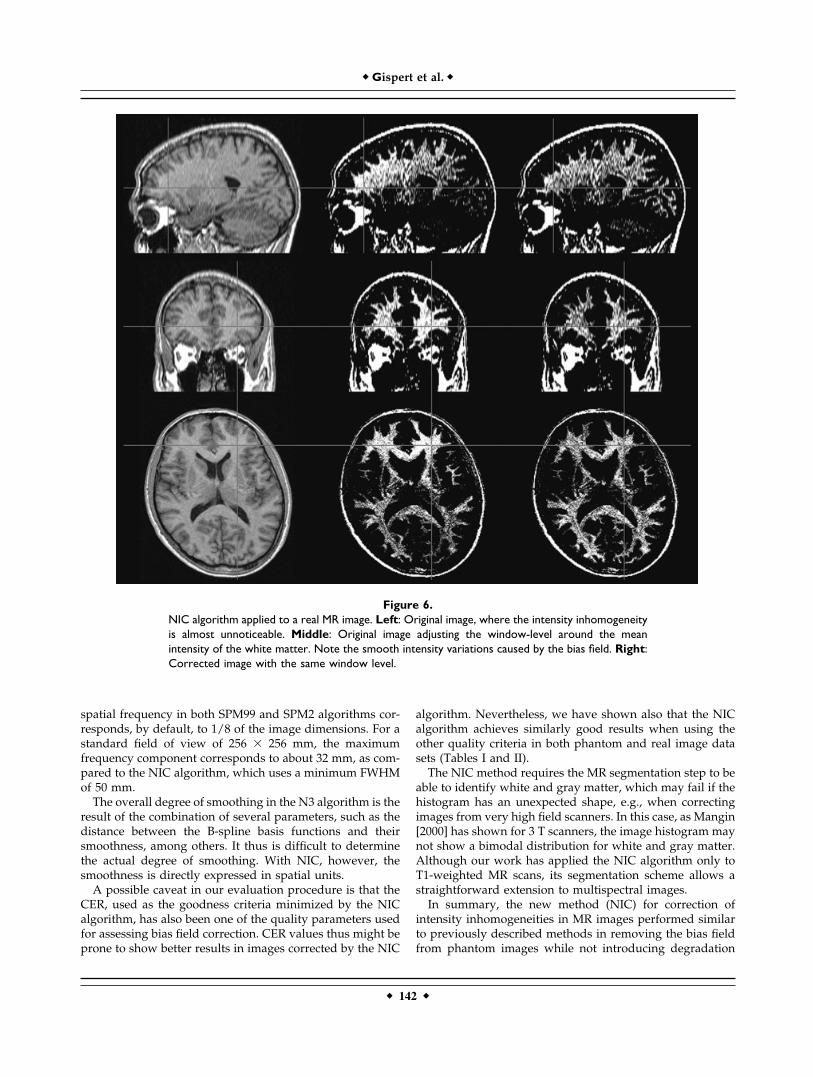
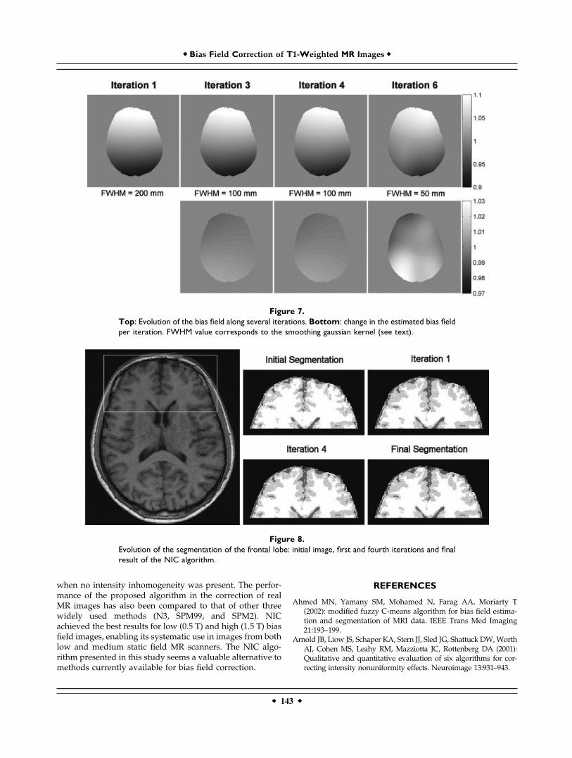
Figure 6 shows an example of MR scan corrected by theNIC algorithm. Figure 7 shows the evolution of the bias fieldestimation through several iterations, and the evolution ofthe corresponding segmentation can be seen in Figure 8.

DISCUSSION

Performance of NIC on Phantom Images

The validation with phantom images used the same meth-odology and datasets used in the reference work of Arnoldet al. [2001], thus enabling a direct comparison with ourresults for the NIC algorithm. Arnold et al. [2001] showed

that both N3 and BFC achieved the best performance whencorrecting the paraboloidal bias field (correlation coefficientbetween applied versus extracted fields, r � 0.98). N3yielded the best results in the removal of the sinusoidal field(r � 0.96), and the HUM method introduced lower degra-dation when correcting phantom images without bias field(r � 0.999).

Comparing the applied versus extracted bias fields (Fig.5), the NIC algorithm obtained the same correlation coeffi-cient (r � 0.98) as N3 and BFC did for the �8% parabolic biasfield. The NIC algorithm also achieved the same quality asthat of the N3 method in the correction of the �8% sinusoi-dal bias field (r � 0.96). When correcting phantom imageswithout bias field, the NIC method showed better results (r� 1.000) than did HUM (r � 0.999) and N3 (r � 0.997).Although it is debatable whether such small differences inthe performance of the different methods on phantom im-ages are relevant in practice, the performance of NIC hasproven to be as good as that of the best available methods.

Summarizing the phantom-based evaluation in a varietyof bias field conditions, it can be stated that the NIC algo-rithm showed better performance in correcting the bias fieldthan did the methods evaluated in Arnold et al. [2001] andwas the only one that did not introduce degradation whenno bias field was present.

Performance of NIC on Real Images

Regardless of the promising results obtained using phan-tom images, the potential usefulness of the NIC algorithmshould be evaluated in the scope of practical applications oftissue segmentation of real sets of images. Our experimentalsetup allowed us to test the algorithm in high and low biasfield conditions. The comparison of the performance in re-ducing the segmentation error achieved by the five methods

TABLE II. Mean and range of the four quality criteria

Method CVWM (%) CVGM (%) CJVWG (%) CER (%)

0.5 T (n � 12)Uncorrected 5.39 (4.81, 5.96) 15.12 (13.27, 17.36) 108.75 (100.50, 138.71) 10.29 (9.40, 13.81)SPM99-L 9.14 (5.03, 34.77) 14.59 (10.60, 20.40) 129.15 (116.17, 177.92) 11.14 (10.49, 16.15)SPM99-S 10.13 (4.71, 33.82) 13.54 (10.17, 17.48) 132.03 (110.65, 170.94) 10.83 (9.63, 17.37)SPM2 5.29 (4.63, 6.24) 19.19 (10.73, 25.72) 122.17 (102.62, 156.21) 10.53 (9.38, 15.34)N3 5.15 (4.55, 5.42) 14.29 (12.90, 16.71) 113.65 (105.27, 135.79) 10.51 (9.73, 14.36)NIC 5.02 (4.39, 5.29) 14.48 (12.73, 16.56) 105.81 (99.84, 126.69) 9.79 (8.86, 13.44)1.5 T (n � 12)Uncorrected 6.52 (5.79, 7.59) 16.75 (12.74, 20.74) 83.92 (76.37, 97.10) 9.08 (8.74, 12.79)SPM99-L 6.26 (4.70, 7.41) 17.34 (14.44, 21.49) 105.97 (86.30, 135.33) 12.90 (10.08, 18.87)SPM99-S 5.53 (4.57, 6.22) 16.31 (13.80, 19.89) 93.40 (78.19, 107.37) 10.61 (8.99, 14.64)SPM2 7.50 (5.39, 8.67) 15.97 (12.00, 20.52) 88.69 (76.80, 99.76) 9.77 (8.69, 12.37)N3 5.88 (5.36, 6.45) 16.47 (14.75, 19.82) 83.95 (77.03, 91.37) 8.84 (8.15, 11.39)NIC 5.84 (5.30, 6.57) 15.70 (12.32, 19.88) 80.77 (74.95, 88.85) 8.04 (7.18, 10.96)

Coefficient of variation of white matter (CVWM), coefficient of variation of the gray matter (CVGM), coefficient of joint variation of white andgray matter (CJVWG), and classification error rate (CER) in the uncorrected original and corrected real images when using the SPM99, SPM2,N3, and NIC methods. Lower values denote lower bias field in the images.


� 140 �

tested (SPM99-S, SPM99-L, SPM2, N3, and NIC) suggestedthat the NIC algorithm was the more efficient method, as itconsistently showed better values for all four quality criteria(Table II). The SPM99-S and N3 methods, compared to theNIC algorithm, achieved a higher reduction of the CVGM inthe 0.5 T images. The SPM99-S method also yielded a betterresult for the CVWM for 0.5 T images. CJVWG and CERvalues, however, showed worse results for those methods,reaching an overall performance below that of the NICalgorithm.

Regarding the robustness of the different algorithms inlow bias field conditions (at 0.5 T), NIC was the only methodthat did not degrade the original scans, still reducing thesegmentation error with respect to the initial images (TableII). A possible reason for the worse results on 0.5 T imagesmay be the lower contrast of these images. Our method,however, performed better than the others did without anyparticular tuning for this type of images. This result enablesa systematic use of NIC in images with either intense or mildbias field artifact.

Regarding the consequences of the bias field correction onthe quality of the segmentation, Chard et al. [2002] foundsignificant improvement of the reproducibility of volumemeasurements of brain tissues after correcting intensity in-homogeneities with the SPM99 algorithm. An improvementin reproducibility of such measurements thus is expectedalso when using our method, given its superior performancewith respect to SPM99.

The smoothing carried out on the bias field estimate had asignificant impact on the results of the correction method.Conventional filtering techniques are unsatisfactory for thisapplication due to boundary effects that significantly de-grade overall performance [Sled et al., 1998]. Most standardmethods model the bias field with low spatial frequencyfunctions, such as a discrete cosine set [Ashburner and Fris-ton, 2000; Ashburner, 2002], low order polynomials [Likar etal., 2001; Van Leemput et al., 1999a] or 3-D splines [Sled etal., 1998]. The NIC algorithm uses a gaussian kernel tosmooth the “residual” image. The degree of smoothing is atunable parameter in all these methods; the highest bias field

Figure 5.Scatterplots and correlation coefficients between theapplied versus extracted bias on phantom imagescontaining �8% paraboloidal bias field (a), �8% sinu-soidal bias field (b), and no bias field (c).


� 141 �

spatial frequency in both SPM99 and SPM2 algorithms cor-responds, by default, to 1/8 of the image dimensions. For astandard field of view of 256 256 mm, the maximumfrequency component corresponds to about 32 mm, as com-pared to the NIC algorithm, which uses a minimum FWHMof 50 mm.

The overall degree of smoothing in the N3 algorithm is theresult of the combination of several parameters, such as thedistance between the B-spline basis functions and theirsmoothness, among others. It thus is difficult to determinethe actual degree of smoothing. With NIC, however, thesmoothness is directly expressed in spatial units.

A possible caveat in our evaluation procedure is that theCER, used as the goodness criteria minimized by the NICalgorithm, has also been one of the quality parameters usedfor assessing bias field correction. CER values thus might beprone to show better results in images corrected by the NIC

algorithm. Nevertheless, we have shown also that the NICalgorithm achieves similarly good results when using theother quality criteria in both phantom and real image datasets (Tables I and II).

The NIC method requires the MR segmentation step to beable to identify white and gray matter, which may fail if thehistogram has an unexpected shape, e.g., when correctingimages from very high field scanners. In this case, as Mangin[2000] has shown for 3 T scanners, the image histogram maynot show a bimodal distribution for white and gray matter.Although our work has applied the NIC algorithm only toT1-weighted MR scans, its segmentation scheme allows astraightforward extension to multispectral images.

In summary, the new method (NIC) for correction ofintensity inhomogeneities in MR images performed similarto previously described methods in removing the bias fieldfrom phantom images while not introducing degradation

Figure 6.NIC algorithm applied to a real MR image. Left: Original image, where the intensity inhomogeneityis almost unnoticeable. Middle: Original image adjusting the window-level around the meanintensity of the white matter. Note the smooth intensity variations caused by the bias field. Right:Corrected image with the same window level.


� 142 �

when no intensity inhomogeneity was present. The perfor-mance of the proposed algorithm in the correction of realMR images has also been compared to that of other threewidely used methods (N3, SPM99, and SPM2). NICachieved the best results for low (0.5 T) and high (1.5 T) biasfield images, enabling its systematic use in images from bothlow and medium static field MR scanners. The NIC algo-rithm presented in this study seems a valuable alternative tomethods currently available for bias field correction.

REFERENCES

Ahmed MN, Yamany SM, Mohamed N, Farag AA, Moriarty T(2002): modified fuzzy C-means algorithm for bias field estima-tion and segmentation of MRI data. IEEE Trans Med Imaging21:193–199.

Arnold JB, Liow JS, Schaper KA, Stern JJ, Sled JG, Shattuck DW, WorthAJ, Cohen MS, Leahy RM, Mazziotta JC, Rottenberg DA (2001):Qualitative and quantitative evaluation of six algorithms for cor-recting intensity nonuniformity effects. Neuroimage 13:931–943.

Figure 8.Evolution of the segmentation of the frontal lobe: initial image, first and fourth iterations and finalresult of the NIC algorithm.

Figure 7.Top: Evolution of the bias field along several iterations. Bottom: change in the estimated bias fieldper iteration. FWHM value corresponds to the smoothing gaussian kernel (see text).


� 143 �

Ashburner J (2002): Another MRI bias correction approach. In: 8thInternational Conference on Functional Mapping of the HumanBrain, 25–28 September, Sendai, Japan.

Ashburner J, Friston K (1997): Multimodal image coregistration andpartitioning: a unified framework. Neuroimage 6:209–217.

Ashburner J, Friston KJ (2000): Voxel-based morphometry: themethods. Neuroimage 11:805–821.

Atkins MS, Mackiewich BT (1998): Fully automatic segmentation ofthe brain in MRI. IEEE Trans Med Imaging 17:98–107.

Brinkmann BH, Manduca A, Robb RA (1998): Optimized homomor-phic unsharp masking for MR grayscale inhomogeneity correc-tion. IEEE Trans Med Imaging 17:161–171.

Brummer ME, Mersereau RM, Eisner RL, Lewine RR (1993): Auto-matic detection of brain contours in MRI datasets. IEEE TransMed Imaging 12:153–166.

Chard DT, Parker GJ, Griffin CMB, Thompson AJ, Miller DH (2002):The reproducibility and sensitivity of brain tissue volume mea-surements derived from an SPM-based segmentation methodol-ogy. J Magn Reson Imaging 15:259–267.

Cohen MS, DuBois RM, Zeineh MM (2000): Rapid and effectivecorrection of RF inhomogeneity for high field magnetic reso-nance imaging. Hum Brain Mapp 10:204–211.

Collins DL, Zijdenbos AP, Kollokian V, Sled JG, Kabani NJ, HolmesCJ, Evans AC (1998): Design and construction of a realisticdigital brain phantom. IEEE Trans Med Imaging 17:463–468.

Cusack R, Brett M, Osswald K (2003): An evaluation of the use ofmagnetic field maps to undistort echo-planar images. Neuroim-age 18:127–142.

Dawant BM, Zijdenbos AP, Margolin RA (1993): Correction of in-tensity variations in MR images for computer-aided tissue clas-sification. IEEE Trans Med Imaging 12:770–781.

DeCarli C, Murphy DGM, Teichberg D, Campbell G, Sobering GS(1996): Local histogram correction of MRI spatially dependentimage pixel intensity nonuniformity. J Magn Reson Imaging6:519–528.

Deichmann R, Good CD, Turner R (2002): RF inhomogeneity compen-sation in structural brain imaging. Magn Reson Med 47:398–402.

Dempster AP, Laird NM, Rubin DB (1977): Maximum likelihood fromincomplete data via the EM algorithm. J R Stat Soc 39:1–38.

Good CD, Scahill RI, Fox NC, Ashburner J, Friston KJ, Chan D,Crum WR, Rossor MN, Frackowiak RS (2002): Automatic differ-entiation of anatomical patterns in the human brain: validationwith studies of degenerative dementias. Neuroimage 17:29–46.

Guillemaud R, Brady M (1997): Estimating the bias field of MRimages. IEEE Trans Med Imaging 16:238–251.

Johnston B, Atkins MS, Mackiewich B, Anderson M (1996): Segmen-tation of multiple sclerosis lesions in intensity corrected multi-spectral MRI. IEEE Trans Med Imaging 15:154–169.

Lawrie SM, Abukmeil SS (1998): Brain abnormality in schizophre-nia. A systematic and quantitative review of volumetric mag-netic resonance imaging studies. Br J Psychiatry 172:110–120.

Likar B, Viergever MA, Pernus F (2001): Retrospective correction ofMR intensity inhomogeneity by information minimization. IEEETrans Med Imaging 20:1398–1410.

Mangin JF (2000): Entropy minimization for automatic correction ofintensity nonuniformity. In: IEEE workshop in mathematicalmethods in biomedical image analysis. Hilton Head Island. SC:IEEE Press. p 162–169.

Marroquin JL, Vemuri BC, Botello S, Calderon F, Fernandez-BouzasA (2002): An accurate and efficient bayesian method for auto-matic segmentation of brain MRI. IEEE Trans Med Imaging21:934–945.

Miller DH, Barkhof F, Frank JA, Parker GJ, Thompson AJ (2002):Measurement of atrophy in multiple sclerosis: pathological ba-sis, methodological aspects and clinical relevance. Brain 125:1676–1695.

Pham DL, Prince JL (1999): Adaptive fuzzy segmentation of mag-netic resonance images. IEEE Trans Med Imaging 18:737–752.

Ruan S, Jaggi C, Xue J, Fadili J, Bloyet D (2000): Brain tissue classi-fication of magnetic resonance images using partial volumemodeling. IEEE Trans Med Imaging 19:1179–1187.

Santago P, Gage HD (1995): Statistical models of partial volumeeffect. IEEE Trans Image Process 4:1531–1540.

Schomberg H (1999): Off-resonance correction of MR images. IEEETrans Med Imaging 18:481–495.

Shattuck DW, Sandor-Leahy SR, Schaper KA, Rottenberg DA,Leahy RM (2001): Magnetic resonance image tissue classificationusing a partial volume model. Neuroimage 13:856–876.

Simmons A, Tofts PS, Barker GJ, Arridge SR (1994): Sources ofintensity nonuniformity in spin echo images at 1.5 T. MagnReson Med 32:121–128.

Sled JG, Pike GB (1998): Standing-wave and RF penetration artifactscaused by elliptic geometry: an electrodynamic analysis of MRI.IEEE Trans Med Imaging 17:653–662.

Sled JG, Zijdenbos AP, Evans AC (1998): A nonparametric methodfor automatic correction of intensity nonuniformity in MRI data.IEEE Trans Med Imaging 17:87–97.

Stokking R, Vincken KL, Viergever MA (2000): Automatic morphol-ogy-based brain segmentation (MBRASE) from MRI-T1 data.Neuroimage 12:726–738.

Van Leemput K, Maes F, Vandermeulen D, Suetens P (1999a):Automated model-based bias field correction of MR images ofthe brain. IEEE Trans Med Imaging 18:885–896.

Van Leemput K, Maes F, Vandermeulen D, Suetens P (1999b):Automated model-based tissue classification of MR images ofthe brain. IEEE Trans Med Imaging 18:897–908.

Velthuizen RP, Cantor AB, Lin H, Fletcher LM, Clarke LP (1998):Review and evaluation of MRI nonuniformity correction forbrain tumor response measurements. Med Phys 25:1655–1666.

Vokurka EA, Thacker NA, Jackson A (1999): A fast model indepen-dent method for automatic correction of intensity nonuniformityin MRI data. J Magn Reson Imaging 10:550–562.

Vokurka EA, Watson NA, Watson Y, Thacker NA, Jackson A (2001):Improved high resolution MR imaging for surface coils usingautomated intensity non-uniformity correction: feasibility studyin the orbit. J Magn Reson Imaging 14:540–546.

Weinberger DR, McClure RK (2002): Neurotoxicity, neuroplastic-ity, and magnetic resonance imaging morphometry: what ishappening in the schizophrenic brain? Arch Gen Psychiatry59:553–558.

Wells WM, Grimson WEL, Kikinis R, Jolesz FA (1996): Adaptivesegmentation of MRI data. IEEE Trans Med Imaging 15:429 –442.

Zhang Y, Brady M, Smith S (2001): Segmentation of brain MRimages through a hidden Markov random field model and theexpectation-maximization algorithm. IEEE Trans Med Imaging20:45–57.


� 144 �

Documents

Method for Bias Field Correction of Brain T1-Weighted Magnetic