Gaspar and Breen BMC Bioinformatics (2019) 20:116 https://doi.org/10.1186/s12859-019-2680-1

METHODOLOGY ARTICLE Open Access

Probabilistic ancestry maps: a methodto assess and visualize populationsubstructures in geneticsHéléna A. Gaspar1,2* and Gerome Breen1,2

Abstract

Background: Principal component analysis (PCA) is a standard method to correct for population stratification inancestry-specific genome-wide association studies (GWASs) and is used to cluster individuals by ancestry. Using the1000 genomes project data, we examine how non-linear dimensionality reduction methods such as t-distributedstochastic neighbor embedding (t-SNE) or generative topographic mapping (GTM) can be used to provide improvedancestry maps by accounting for a higher percentage of explained variance in ancestry, and how they can help toestimate the number of principal components necessary to account for population stratification. GTM generatesposterior probabilities of class membership which can be used to assess the probability of an individual to belong to agiven population - as opposed to t-SNE, GTM can be used for both clustering and classification.

Results: PCA only partially identifies population clusters and does not separate most populations within a givencontinent, such as Japanese and Han Chinese in East Asia, or Mende and Yoruba in Africa. t-SNE and GTM, taking intoaccount more data variance, can identify more fine-grained population clusters. GTM can be used to buildprobabilistic classification models, and is as efficient as support vector machine (SVM) for classifying 1000 GenomesProject populations.

Conclusion: The main interest of probabilistic GTM maps is to attain two objectives with only one map: provide abetter visualization that separates populations efficiently, and infer genetic ancestry for individuals or populations.This paper is a first application of GTM for ancestry classification models. Our code (https://github.com/hagax8/ancestry_viz) and interactive visualizations (https://lovingscience.com/ancestries) are available online.

Keywords: Generative topographic mapping, Ancestry, Genetics, Population stratification

BackgroundAs of 2018, most genome-wide association studies(GWASs) have used populations of European ancestry.However, larger sample sizes are now available and bothsocietal need and funders are mandating more studiesfocused on other populations. Visualizing and accuratelydefining complex population structure is therefore ofparamount importance. In this paper, we have three aims:to find a better way to visualize population substructures,

*Correspondence: helena.gaspar@kcl.ac.uk1King’s College London; Institute of Psychiatry, Psychology and Neuroscience;Social, Genetic and Developmental Psychiatry (SGDP) Centre, 16 De CrespignyPark, SE5 8AF London, UK2National Institute for Health Research Biomedical Research Centre; SouthLondon and Maudsley National Health Service Trust, London, UK

to define a new procedure to estimate the optimal numberof principal components accounting for population strati-fication, and to obtain an ancestry classification algorithmwhich can also estimate probabilities to belong to differentancestry groups. This paper focuses on global (genome-wide) ancestry rather than local ancestry defined withinchromosome segments.Principal component analysis (PCA) is widely used

to investigate population structure in genetics [1], andto account for population stratification in GWASs (cf.EIGENSTRAT software [2]). However, the 2 or 3 principalcomponents used to build a PCA plot generally accountfor a small percentage of variance explained and leadto a simplified visualization of population substructures,focused on major continental ancestry, with only partial

© The Author(s). 2019 Open Access This article is distributed under the terms of the Creative Commons Attribution 4.0International License (http://creativecommons.org/licenses/by/4.0/), which permits unrestricted use, distribution, andreproduction in any medium, provided you give appropriate credit to the original author(s) and the source, provide a link to theCreative Commons license, and indicate if changes were made. The Creative Commons Public Domain Dedication waiver(http://creativecommons.org/publicdomain/zero/1.0/) applies to the data made available in this article, unless otherwise stated.

Gaspar and Breen BMC Bioinformatics (2019) 20:116 Page 2 of 11

sensitivity for the identification of admixed individualsor more complex ancestry. Model-based methods suchas STRUCTURE [3] and ADMIXTURE [4] provide maxi-mum likelihood estimations of ancestry based on ancestryproportions and allele frequencies but do not provide thesimple 2D maps that can be obtained with PCA, multidi-mensional scaling (MDS), and other multivariate analysismethods.A PCA ancestry map is constructed from a genotype

matrix G of dimension N × D, where the N instances areindividuals and the D features correspond to genetic vari-ants - typically single nucleotide polymorphisms (SNPs)which are pruned to remove SNPs in high linkage dise-quilibrium with each other so that the identified principalcomponents do not reflect local haplotype structure, butinstead reflect genome-wide ancestry. For example, Gndcould be the minor allele count for SNP d in individualn. For visualization purposes, PCA is used to map G to amore interpretable latent or hidden space of 2 or 3 dimen-sions: G → X, where X has dimension N × 2 or N × 3.The new variables - typically two for a PCA plot - are thefirst principal components, which account for the high-est percentage of the overall variance. However, the totalpercentage of variance explained by such a small numberof principal components can be low for high-dimensionalgenotype matrices.More complex visualization methods such as t-

distributed stochastic neighbor embedding (t-SNE) [5]or generative topographic mapping (GTM) [6], whichare manifold-based and non-linear dimensionality reduc-tion algorithms, are able to capture more information byembedding a D-dimensional space in a low-dimensionallatent space, where D can be any number of features.Instead of two or three principal components, any numberof principal components can be used with these methods.To assess the percentage of variance to account for pop-ulation substructures, we propose to execute two map-pings, first carrying out PCA to select principal compo-nents and then using t-SNE or GTM:G → X’ → X, whereX’ is the matrix of F principal components (F > 2), and Xis the final t-SNE or GTM projection in a 2-dimensionalspace. The performance of ancestry classification modelsbuilt withX or the visual assessment of clusters inX couldthen provide a way to estimate the number of principalcomponents to account for population stratification.Both t-SNE and GTM are used for clustering tasks.

However, new instances cannot be projected onto a t-SNEmap without training the map once again. GTM, on theother hand, not only allows for the projection of new datapoints, but comes with a probabilistic framework to builda comprehensive classification model and assign proba-bilities of class membership. t-SNE is now widely used ingenetics, and has already been applied to visual popula-tion stratification [7], transcriptome visualization [8], and

single-cell analysis [9]. GTM is more popular in chemin-formatics, and was used to classify chemical compounds[10] or to compare chemical libraries [11]. GTM couldeasily be transposed to genetics and used to predict ances-try and relative degree of admixture in an individual or agroup.In this paper, 1000 Genomes Project Phase III [12]

data is used to build the genotype matrix G. The 1000Genomes Project has gathered genotypes from 26 dif-ferent populations corresponding to 5 superpopulations:Africans (AFR), Admixed Americans (AMR), East Asians(EAS), Europeans (EUR) and South Asians (SAS). We sep-arated these populations into a training set of 20 popula-tions, and an external test set of 6 populations: Americansof African ancestry in Southwest USA (ASW); AfricanCaribbeans in Barbados (ACB); Mexican ancestry fromLos Angeles USA (MXL); Gujarati Indian from Hous-ton, Texas (GIH); Sri Lankan Tamil from the UK (STU);and Indian Telugu from the UK (ITU). Ancestry mapsare investigated to cluster and visualize superpopulationsand populations using PCA, t-SNE, and GTM. t-SNE andGTM maps accounting for 3 to 1000 principal compo-nents are compared to a simple PCA plot. We also com-pare GTM ancestry classification models to two differentalgorithms: k-nearest neighbors (k-NN) models based onthe 2D PCA plot, and linear Support Vector Machine(SVM), a classical machine learning algorithm [13]. Wealso demonstrate how to assess probabilities of ancestrymembership in individuals and populations using GTM.

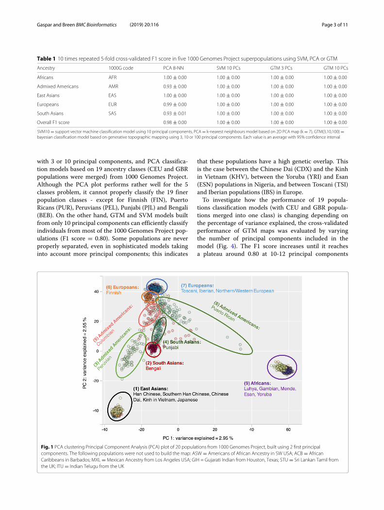
ResultsClassification of 5 superpopulationsVisualizations and complete model performance statisticscan be found in Additional files 1, 2, 3, 4, 5, 6, 7, 8, 9, 10, 11,12, 13, 14. PCA clusters and predicts the 5 superpopula-tions in 1000Genomes Project efficiently (F1 score= 0.98,cf. Table 1 and Fig. 1): Europeans, Africans, South Asians,East Asians, and Admixed Americans. However, SVM andGTM models with 3 or 10 principal components havehigher recall for Admixed Americans and higher precisionfor South Asians (cf. Additional files 13 and 14). Opti-mal performances can be achieved by including a thirdprincipal component.From Figs. 2 and 3, it can be seen that t-SNE and GTM

recognize the same clusters. However, GTM suffers froma packing effect, which results in data points being packedtogether on amap. t-SNE remedies this situation with Stu-dent’s t-distributions in the latent space, which allow smalldistances between data points in the original space to betranslated into larger distances in the 2D latent space.

Classification performances for 19 ancestry classesIn Table 2, we report performance measures (10 timesrepeated 5-fold cross-validated F1 score) for SVM, GTM

Gaspar and Breen BMC Bioinformatics (2019) 20:116 Page 3 of 11

Table 1 10 times repeated 5-fold cross-validated F1 score in five 1000 Genomes Project superpopulations using SVM, PCA or GTM

Ancestry 1000G code PCA 8-NN SVM 10 PCs GTM 3 PCs GTM 10 PCs

Africans AFR 1.00 ± 0.00 1.00 ± 0.00 1.00 ± 0.00 1.00 ± 0.00

Admixed Americans AMR 0.93 ± 0.00 1.00 ± 0.00 1.00 ± 0.00 1.00 ± 0.00

East Asians EAS 1.00 ± 0.00 1.00 ± 0.00 1.00 ± 0.00 1.00 ± 0.00

Europeans EUR 0.99 ± 0.00 1.00 ± 0.00 1.00 ± 0.00 1.00 ± 0.00

South Asians SAS 0.93 ± 0.01 1.00 ± 0.00 1.00 ± 0.00 1.00 ± 0.00

Overall F1 score 0.98 ± 0.00 1.00 ± 0.00 1.00 ± 0.00 1.00 ± 0.00

SVM10 = support vector machine classification model using 10 principal components, PCA = k-nearest neighbours model based on 2D PCA map (k = 7), GTM{3,10,100} =bayesian classification model based on generative topographic mapping using 3, 10 or 100 principal components. Each value is an average with 95% confidence interval

with 3 or 10 principal components, and PCA classifica-tion models based on 19 ancestry classes (CEU and GBRpopulations were merged) from 1000 Genomes Project.Although the PCA plot performs rather well for the 5classes problem, it cannot properly classify the 19 finerpopulation classes - except for Finnish (FIN), PuertoRicans (PUR), Peruvians (PEL), Punjabi (PJL) and Bengali(BEB). On the other hand, GTM and SVM models builtfrom only 10 principal components can efficiently classifyindividuals from most of the 1000 Genomes Project pop-ulations (F1 score = 0.80). Some populations are neverproperly separated, even in sophisticated models takinginto account more principal components; this indicates

that these populations have a high genetic overlap. Thisis the case between the Chinese Dai (CDX) and the Kinhin Vietnam (KHV), between the Yoruba (YRI) and Esan(ESN) populations in Nigeria, and between Toscani (TSI)and Iberian populations (IBS) in Europe.To investigate how the performance of 19 popula-

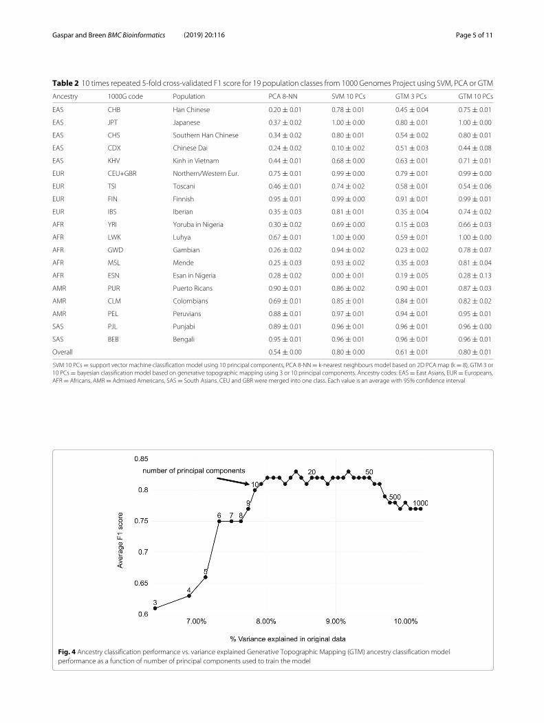
tions classification models (with CEU and GBR popula-tions merged into one class) is changing depending onthe percentage of variance explained, the cross-validatedperformance of GTM maps was evaluated by varyingthe number of principal components included in themodel (Fig. 4). The F1 score increases until it reachesa plateau around 0.80 at 10-12 principal components

Fig. 1 PCA clustering Principal Component Analysis (PCA) plot of 20 populations from 1000 Genomes Project, built using 2 first principalcomponents. The following populations were not used to build the map: ASW = Americans of African Ancestry in SW USA; ACB = AfricanCaribbeans in Barbados; MXL = Mexican Ancestry from Los Angeles USA; GIH = Gujarati Indian from Houston, Texas; STU = Sri Lankan Tamil fromthe UK; ITU = Indian Telugu from the UK

Gaspar and Breen BMC Bioinformatics (2019) 20:116 Page 4 of 11

Fig. 2 GTM clustering with 10 principal components Generative Topographic Mapping (GTM) plot of 20 populations from 1000 Genomes Project,built using 10 first principal components. The following populations were not used to build the map: ASW = Americans of African Ancestry in SWUSA; ACB = African Caribbeans in Barbados; MXL = Mexican Ancestry from Los Angeles USA; GIH = Gujarati Indian from Houston, Texas; STU = SriLankan Tamil from the UK; ITU = Indian Telugu from the UK

Fig. 3 t-SNE clustering with 10 principal components t-distributed stochastic neighbor embedding (t-SNE) plot of 20 populations from 1000Genomes Project, built using 10 first principal components. The following populations were not used to build the map: ASW = Americans of AfricanAncestry in SW USA; ACB = African Caribbeans in Barbados; MXL = Mexican Ancestry from Los Angeles USA; GIH = Gujarati Indian from Houston,Texas; STU = Sri Lankan Tamil from the UK; ITU = Indian Telugu from the UK

Gaspar and Breen BMC Bioinformatics (2019) 20:116 Page 5 of 11

Table 2 10 times repeated 5-fold cross-validated F1 score for 19 population classes from 1000 Genomes Project using SVM, PCA or GTM

Ancestry 1000G code Population PCA 8-NN SVM 10 PCs GTM 3 PCs GTM 10 PCs

EAS CHB Han Chinese 0.20 ± 0.01 0.78 ± 0.01 0.45 ± 0.04 0.75 ± 0.01

EAS JPT Japanese 0.37 ± 0.02 1.00 ± 0.00 0.80 ± 0.01 1.00 ± 0.00

EAS CHS Southern Han Chinese 0.34 ± 0.02 0.80 ± 0.01 0.54 ± 0.02 0.80 ± 0.01

EAS CDX Chinese Dai 0.24 ± 0.02 0.10 ± 0.02 0.51 ± 0.03 0.44 ± 0.08

EAS KHV Kinh in Vietnam 0.44 ± 0.01 0.68 ± 0.00 0.63 ± 0.01 0.71 ± 0.01

EUR CEU+GBR Northern/Western Eur. 0.75 ± 0.01 0.99 ± 0.00 0.79 ± 0.01 0.99 ± 0.00

EUR TSI Toscani 0.46 ± 0.01 0.74 ± 0.02 0.58 ± 0.01 0.54 ± 0.06

EUR FIN Finnish 0.95 ± 0.01 0.99 ± 0.00 0.91 ± 0.01 0.99 ± 0.01

EUR IBS Iberian 0.35 ± 0.03 0.81 ± 0.01 0.35 ± 0.04 0.74 ± 0.02

AFR YRI Yoruba in Nigeria 0.30 ± 0.02 0.69 ± 0.00 0.15 ± 0.03 0.66 ± 0.03

AFR LWK Luhya 0.67 ± 0.01 1.00 ± 0.00 0.59 ± 0.01 1.00 ± 0.00

AFR GWD Gambian 0.26 ± 0.02 0.94 ± 0.02 0.23 ± 0.02 0.78 ± 0.07

AFR MSL Mende 0.25 ± 0.03 0.93 ± 0.02 0.35 ± 0.03 0.81 ± 0.04

AFR ESN Esan in Nigeria 0.28 ± 0.02 0.00 ± 0.01 0.19 ± 0.05 0.28 ± 0.13

AMR PUR Puerto Ricans 0.90 ± 0.01 0.86 ± 0.02 0.90 ± 0.01 0.87 ± 0.03

AMR CLM Colombians 0.69 ± 0.01 0.85 ± 0.01 0.84 ± 0.01 0.82 ± 0.02

AMR PEL Peruvians 0.88 ± 0.01 0.97 ± 0.01 0.94 ± 0.01 0.95 ± 0.01

SAS PJL Punjabi 0.89 ± 0.01 0.96 ± 0.01 0.96 ± 0.01 0.96 ± 0.00

SAS BEB Bengali 0.95 ± 0.01 0.96 ± 0.01 0.96 ± 0.01 0.96 ± 0.01

Overall 0.54 ± 0.00 0.80 ± 0.00 0.61 ± 0.01 0.80 ± 0.01

SVM 10 PCs = support vector machine classification model using 10 principal components, PCA 8-NN= k-nearest neighbours model based on 2D PCA map (k = 8), GTM 3 or10 PCs = bayesian classification model based on generative topographic mapping using 3 or 10 principal components. Ancestry codes: EAS = East Asians, EUR = Europeans,AFR = Africans, AMR = Admixed Americans, SAS = South Asians. CEU and GBR were merged into one class. Each value is an average with 95% confidence interval

Fig. 4 Ancestry classification performance vs. variance explained Generative Topographic Mapping (GTM) ancestry classification modelperformance as a function of number of principal components used to train the model

Gaspar and Breen BMC Bioinformatics (2019) 20:116 Page 6 of 11

accounting for around 8% variance explained. Interest-ingly, beyond 100-200 principal components the perfor-mance starts decreasing. This could be due to includingmore individual-level variance, which would dispersepopulation clusters, or to the curse of dimensionality,which occurs when the number of variables increasesbut not enough data points are provided to populatethe high-dimensional space. This indicates that the num-ber of principal components should be optimized - ourcurve suggests to use 10-12 components for this prunedgenotype matrix.A final map was built with 10 principal components and

the complete training set of 20 populations (cf. Fig. 5). Thesix populations that were not used to build the GTMmapwere used to generate posterior probabilities of super-population membership, which can be interpreted as theprobability for a tested population pop to belong to asuperpopulation: P(AFR|pop) would be the probability ofAfrican ancestry for tested population pop. Results arepresented in Table 3. Indian Telugu from the UK (ITU),Sri Lankan Tamil from the UK (STU), and Gujarati Indianfrom Houston (GIH) are all predicted as South Asianswith P(SAS|pop) = 1 - none of them is mapped to anotherancestry group. Individuals with Mexican ancestry from

Los Angeles (MXL) are mostly mapped as AdmixedAmericans with a small European membership probabil-ity, whereas Americans of African ancestry in SouthwestUSA (ASW) and African Caribbeans in Barbados (ACB)show more mixed results - with high probabilities forboth African and Admixed American superpopulations.Figure 5 shows how Americans of African ancestry inSouthwest USA are distributed on the map: most of themare mapped near the African ancestry group but areassigned to empty nodes, where no African individual inthe training set was mapped; some others are close to theColombian/Peruvian group (AMR 1) and others to thePuerto Rican group (AMR 2).

Additional analysis 1: African-only GTMA separate GTMwas built with African populations exclu-sively (cf. Additional file 15). Americans of African ances-try in Southwest USA (ASW) and Africans Caribbeansin Barbados (ACB) were excluded from the training set,which included: Esan in Nigeria (ESN); Yoruba in Ibadan,Nigeria (YRI); Gambian in Western Divisions in TheGambia (GWD); Luhya in Webuye, Kenya (LWK); andMende in Sierra Leone (MSL). We projected onto thisAfrican-only map ASW and ACB populations, but also

Fig. 5 Projected Americans of African ancestry in Southwest USA (ASW) on a GTMmap. Generative Topographic Map (GTM) trained with 10principal components. Coloured points represent individuals coloured by ancestry or superpopulation (AFR, AMR, EAS, EUR, SAS). Squares representGTM nodes coloured by most probable ancestry. The highlighted black points represent mean positions of ASW individuals projected onto themap. Grey lines map mean positions of individuals on the map to their most probable node. Ancestry codes: EAS = East Asians, EUR = Europeans,AFR = Africans, AMR = Admixed Americans, SAS = South Asians

Gaspar and Breen BMC Bioinformatics (2019) 20:116 Page 7 of 11

Table 3 Posterior probabilities of superpopulation membershipsin 6 test populations obtained by a GTMmodel trained with allsuperpopulations

Population(pop)

P(AFR|pop) P(AMR|pop) P(EAS|pop) P(EUR|pop) P(SAS|pop)

ASW 0.55 0.45 0 0 0

ACB 0.89 0.11 0 0 0

MXL 0 0.98 0 0.02 0

GIH 0 0 0 0 1

STU 0 0 0 0 1

ITU 0 0 0 0 1

NB: GTM classification models are restricted by an applicability domain defined bythe training set. Here, the training set contains twenty 1000 Genomes Project,excluding [ASW, ACB, MXL, GIH, STU, ITU]. These posterior probabilities should beconsidered as a similarity measure between test populations and populations usedto build the map, and not as an absolute measure of population admixture.Abbreviations: ASW = Americans of African Ancestry in SW USA; ACB = AfricanCaribbeans in Barbados; MXL = Mexican Ancestry from Los Angeles USA; GIH =Gujarati Indian from Houston, Texas; STU = Sri Lankan Tamil from the UK; ITU =Indian Telugu from the UK; EUR = Europeans; EAS = East Asians; AMR = AdmixedAmericans; SAS = South Asians

other superpopulations (EUR, EAS, SAS, AMR), in orderto distinguish populations based on their African varia-tion. ASW and ACB are both mapped near Nigerian pop-ulations, whereas all other superpopulations (EUR, EAS,SAS, and AMR) are mapped in the same approximatelocation near the Luhya (LWK) - posterior probabilitiesof ancestry membership are provided in Table 4. How-ever, these superpopulations are mapped in locations thatare not populated by the training set; no strong conclu-sion should be inferred from these results. Moreover, the1000 Genomes Project does not contain many Africanethnic groups. Constructing an African-only map with

Table 4 Posterior probabilities of African ethnicity membershipin 6 test populations obtained by a GTMmodel trained onAfrican populations exclusively

Population(pop)

P(ESN|pop) P(YRI|pop) P(GWD|pop) P(LWK|pop) P(MSL|pop)

ASW 0.24 0.37 0.11 0.13 0.14

ACB 0.29 0.42 0.07 0.07 0.15

EUR 0.04 0.10 0.21 0.62 0.04

EAS 0.09 0.19 0.21 0.44 0.07

AMR 0.07 0.15 0.23 0.49 0.06

SAS 0.06 0.13 0.21 0.53 0.05

NB: GTM classification models are restricted by an applicability domain defined bythe training set. Here, the training set contains only African populations, excludingASW and ACB subsets. These posterior probabilities should be considered as asimilarity measure between test populations and populations used to build themap, and not as an absolute measure of population admixture. Abbreviations: ASW= Americans of African Ancestry in SW USA; ACB = African Caribbeans in Barbados;ESN = Esan in Nigeria; YRI = Yoruba in Ibadan; Nigeria; GWD = Gambian in WesternDivisions in the Gambia; LWK = Luhya in Webuye, Kenya; MSL = Mende in SierraLeone; EUR = Europeans; EAS = East Asians; AMR = Admixed Americans; SAS =South Asians

more ethnic groups would be an interesting follow-up tothis analysis.

Additional analysis 2: Arabidopsis thalianaTo test our methods on non-human genomes, we gener-ated GTM, t-SNE and PCA maps for 1135 Arabidopsisthaliana genomes (a model plant organism) from the 1001Genomes Consortium [14]. Visualizations are available inAdditional files 16 and 17. PCA can separate the strainsby continent but not by individual countries, as opposedto GTM and t-SNE, which find more fine-grained clusterscorresponding to individual countries or regions, suchas Spain, Southern Sweden, Northern Sweden, SouthernItaly, or Northern Italy.

DiscussionDefining the training setOur classification models were trained using knownancestry labels and a reference population (1000 GenomesProject). However, any other reference population couldbe used as a training set. In this application, populationsexpected to be more homogeneous were included in thetraining set. The choice of training set populations couldalso depend on the goal of the study, such as distinguishingbetween African populations in an African-only dataset,in which case a better classification model could be builtusing exclusively African samples.

Testing new dataTo predict the ancestry of new individuals (test set) usinga model trained on a reference population (training set),SNPs in the test matrix should correspond to the SNPs inthe train matrix. This was not an issue in this paper, wherepopulations from 1000 Genomes Project were used forboth training and test. But in the more general case, manyof the SNPs in the training set will be missing from the testset. Missing values in the test matrix should be imputedusing the reference population, which can be achievedusing genome imputation softwares such asMaCH [15] orIMPUTE2 [16].

OutliersGTM or t-SNE maps can also be used to identify ancestryoutliers, i.e. mislabeled individuals. Outliers are typicallymapped to single points far away from their expectedclusters. These data points should be removed from thetraining set used to build the classification model. Byobserving t-SNE and GTM maps, outliers can readily beidentified in the 1000 Genomes Project.

Hyperparameter optimizationOne major drawback of GTM and t-SNE is hyperparam-eter optimization. GTM has at least four hyperparam-eters to optimize, and t-SNE at least three. The maps

Gaspar and Breen BMC Bioinformatics (2019) 20:116 Page 8 of 11

presented in this paper have fixed hyperparameters (cf.Methods). However, hyperparameters might have a sig-nificant impact on the shape of the map, and can beoptimized to obtain better visualization and classifica-tion performance. For GTM classification models, typicalperformance measures such as the F1 score, balancedaccuracy, area under the curve (AUC) or Matthews corre-lation coefficient (MCC) can be used to select the optimalvalues for these hyperparameters.

ConclusionPCA provides a good visualization of the superpopula-tions in the 1000 Genomes Project (AFR, AMR, EUR,EAS, SAS), but is not ideal for more fine-grained cluster-ing and does not provide probabilistic models for admixedpopulations. On the other hand, both t-SNE and GTMprovide a way to cluster and visualize more complex pop-ulation substructures. GTM, as opposed to t-SNE, can beharnessed to generate comprehensive ancestry classifica-tion models. Moreover, new individuals can be directlyprojected onto a pre-constructed GTM map - whichmakes it the ideal choice to cluster individuals based onpre-defined panels. We showed how to assess ancestrymembership probabilities using GTM and interpret themthrough visualization. By generating t-SNE or GTMmapswith increasing number of principal components, we canestimate the percentage of variance explained to iden-tify population substructures - this could also be usefulto account for population stratification in genome-wideassociation studies.

MethodsData and quality controlGenotypes of 2504 people in the 1000 GenomesProject Phase III were downloaded fromftp://ftp.1000genomes.ebi.ac.uk/vol1/ftp/release/20130502[12]. Variants were removed based on a Hardy-Weinbergequilibrium exact test p-value filter (< 0.001) andgenotyping rate filter (> 0.02). The Hardy-Weinbergequilibrium test measures whether the ratio betweenhomozygous and heterozygous genotypes differs sig-nificantly from prediction under HWE assumptions.SNPs from the major histocompatibility complex (MHC)on chromosome 6 and in the chromosome 8 inversionregion were excluded. The remaining SNPs were prunedtwice using plink 1.9 [17, 18] with windows of 1000variants and step size 10, pair-wise squared correlationthreshold = 0.02, and minor allele frequency > 0.05.The pruning operation deals with linkage desequilibriumor non-random association of alleles at different loci:it reduces the number of SNPs, keeps SNPs in linkageequilibrium, and thereby reduces data dimensionality. Atraining set was built by removing the following popula-tions: Americans of African ancestry in Southwest USA

(code = ASW); African Caribbeans in Barbados (ACB);Mexican ancestry from Los Angeles USA (MXL); GujaratiIndian from Houston, Texas (GIH); Sri Lankan Tamilfrom the UK (STU); and Indian Telugu from the UK(ITU). We used these populations as an external test setto predict the degree of relative admixture in individualsand populations. For the classification models, we alsomerged British in England and Scotland (GBR) and UtahResidents with Northern and Western European Ances-try (CEU) to obtain a single category for Northern andWestern European Ancestry.

Additional dataset: Arabidopsis thalianaWe used an additional dataset of 1135 Arabidopsisthaliana genomes extracted from the 1001 GenomesProject [14]; the genotypes and an imputed SNP matrixcould be downloaded from 1001genomes.org. Arabidop-sis thaliana was the first plant genome to be sequencedand is a commonly used model organism. Variants wereremoved using a permissive genotyping rate filter (> 0.2).SNPs were pruned using plink 1.9 [17, 18] with windowsof 100 variants and step size 10, pair-wise squared corre-lation threshold = 0.1, and minor allele frequency >0.05.We merged the imputed SNP matrix with our filtered listof SNPs to obtain a filtered imputed SNP matrix.

Visualization of ancestry clusters using t-SNE and GTMt-SNE [5] translates similarities between points into prob-abilities; Gaussian joint probabilities in the original inputspace and Student’s t-distributions in the latent space. TheKullback-Leibler divergence between data distributions inthe input and latent space is minimized with gradientdescent. t-SNE has several parameters to optimize: thelearning rate for gradient descent, the perplexity of dis-tributions in the initial space, and the early exaggeration.In this paper, we used the scikit-learn v0.19.1 implemen-tation for t-SNE [19], with default learning rate = 200,perplexity = 30, and early exaggeration = 12. The maindisadvantage of t-SNE is its lack of a framework to projectnew points onto a pre-trained map - a feature available inPCA and GTM.The core principle of GTM [6] is to fit a manifold into

the high-dimensional initial space. The points yk on themanifold Y in the initial space are the centers of normalprobability distributions of g, which here are individualsdescribed by the genotype matrix G:

p(g|xk ,W,β) = β

2π

D/2exp

(−β

2‖yk − g‖2

)(1)

where β is the common inverse variance of these dis-tributions and W is the parameters matrix of the map-ping function y(x;W) which maps nodes xk in the latentspace to yk : y(xk ;W) = Wφ(xk), where φ(xk) is a setof radial basis functions. W and β are optimized with

Gaspar and Breen BMC Bioinformatics (2019) 20:116 Page 9 of 11

an expectation-maximization (EM) algorithm maximiz-ing the overall data likelihood. The responsibility or pos-terior probability that the individual gn in the originalgenotype space is generated from the kth node in thelatent space is computed using Bayes theorem:

Rkn = p(xk|gn,W,β) = p(gn|xk ,W,β)p(xk)∑Kk′=1 p(gn|xk′ ,W,β)p(xk′)

(2)

These responsibilities are used to compute the mean posi-tion of an individual on the map x(gn), by averaging overall nodes on the map:

x(gn) =K∑

k=1xkRkn (3)

We used the python package ugtm v1.1.4 [20] for gen-erative topographic mapping, and scripts used for ances-try classification are available online (https://github.com/hagax8/ancestry_viz). GTM has several hyperparametersto tune, which might have a high impact on the shape ofthe map: the number of radial basis functions, a width fac-tor for these functions, map grid size, and a regularizationparameter.

Ancestry classification modelsPCA does not provide a comprehensive framework tobuild a probabilistic classification model. However, a sim-ple classification model associated with the 2-dimensionalplot can be built using the k-NN approach in three steps:(1) a PCA plot is constructed from a training set, (2) a testset is projected on the plot, and (3) each test individual isassigned the predominant ancestry amongst its k nearestneighbors in the training set. We did not construct k-NNmodels for t-SNE since it is not straightforward to projectnew points onto a t-SNE map. On the other hand, GTMprovides a probabilistic framework which can be used tobuild classification models and generate class member-ship probabilities [10]. GTM responsibilities can be seenas feature vectors: they encode individuals depending ontheir position on the map, which is discretized into a finitenumber of nodes (positions). They can be used to estimatethe probability of a specific ancestry given the position onmap, using Bayes’ theorem

P(a|xk) = P(xk|a) × P(a)∑a P(xk|a) × P(a)

(4)

where P(xk|a) is computed as follows:

P(xk|a) =∑

n RknNa

(5)

where Rkn is the responsibility of node xk for an individualbelonging to population a, which countsNa individuals. It

is then possible to predict the ancestry profile P(a|gi) of anew individual with associated responsibilities {Rki}

P(a|gi) =∑k

P(a|xk) × Rki (6)

GTM nodes xk can be represented as points coloured bymost probable ancestry amax using P(amax|xk). We com-pared performances of visual classifications (PCA andGTM) with linear support vector machine classification(SVM), a classical machine learning algorithm. LinearSVM is only dependent on C, the penalty hyperparame-ter. Increasing C increases the variance of the model anddecreases its bias. In this application, classification per-formance is estimated by the average F1 score over allancestry classes in a 5-fold cross-validation experiment(5-CV) repeated 10 times. The F1 score is a harmonicmean of precision and recall. For each of the 10 repe-titions, labels are predicted for 5 partitions of the data,which are concatenated to obtain predicted values for theentire dataset. From these, F1 scores are computed foreach class a and repetition j. The per-class performancemeasure is computed across the 10 repetitions:

F1scorea =

10∑j=1

F1scoreaj

10(7)

The overall model performance measure is a weightedaverage across per-class F1 scores, with weights equal tothe number of individuals in the class:

F1score =⎛⎝ 10∑

j=1

∑aF1scoreaj × Na

Ntotal

⎞⎠ ÷ 10 (8)

This procedure is performed for each parameter combina-tion and for each algorithm (PCA, GTM, SVM). The bestmodel for each algorithm is defined as having the largestoverall F1 score. Only the performance of the best modelis reported in the Results section. For PCA, we vary k (thenumber of neighbours) from 1 to 10. For GTM, we set themap grid size (number of nodes) = 16*16, the number ofRBFs = 4*4, regularization = 0.1 and rbf width factor =0.3. For linear SVM, the penalty parameter is set toC = 2rwhere r runs from -5 to 10.

Posterior probabilities of ancestry membership for wholepopulationsAll our models are trained with only twenty 1000Genomes Project populations. Six populations are used asan external test set (cf. foregoing section Data and qualitycontrol). Posterior probabilities of ancestry membershipare estimated for all individuals in these test populations(Eq. 6) based on observed superpopulation distributions

Gaspar and Breen BMC Bioinformatics (2019) 20:116 Page 10 of 11

(Eq. 5). We also generate probabilities of belonging to asuperpopulation for each population as a whole, by replac-ing individual responsibilities {Rki} in equation 6 by anoverall population responsibility {Rkp}

Rkp =∑

i RkiNi

(9)

It should be noted that these responsibilities {Rkp} corre-spond to the averaged distribution of the population onthe map, and can be used to compare populations andestimate their diversity.

Additional files

Additional file 1: GTMmap of twenty 1000 Genomes Projectpopulations. Interactive GTM map of twenty 1000 Genomes Projectpopulations. File name: 1000G_GTM_20populations.html. The file can beviewed in a web browser with internet access. (HTML 2416 kb)

Additional file 2: t-SNE map of twenty 1000 Genomes Projectpopulations. Interactive t-SNE map of twenty 1000 Genomes Projectpopulations. File name: 1000G_t-SNE_20populations.html. The file can beviewed in a web browser with internet access. (HTML 589 kb)

Additional file 3: GTM projection, test set 1: Americans of African ancestryin SW USA (ASW). Projection of Americans of African ancestry in SW USA(black points) onto a GTM map trained with 10 principal components. Filename: 1000G_GTM_projection_ASW.html. The file can be viewed in a webbrowser with internet access. (HTML 437 kb)

Additional file 4: GTM projection, test set 2: African Caribbeans inBarbados (ACB). Projection of African Caribbeans in Barbados (black points)onto a GTM map trained with 10 principal components. File name:1000G_GTM_projection_ACB.html. The file can be viewed in a webbrowser with internet access. (HTML 471 kb)

Additional file 5: GTM projection, test set 3: Mexican Ancestry from LosAngeles USA (MXL). Projection of individuals of Mexican ancestry from LosAngeles USA (black points) onto a GTM map trained with 10 principalcomponents. File name: 1000G_GTM_projection_MXL.html. The file can beviewed in a web browser with internet access. (HTML 439 kb)

Additional file 6: GTM projection, test set 4: Gujarati Indian from Houston,Texas (GIH). Projection of Gujarati Indian from Houston (black points) ontoa GTM map trained with 10 principal components. File name:1000G_GTM_projection_GIH.html. The file can be viewed in a webbrowser with internet access. (HTML 483 kb)

Additional file 7: GTM projection, test set 5: Sri Lankan Tamil from the UK(STU). Projection of Sri Lankan Tamil from the UK (black points) onto a GTMmap trained with 10 principal components. File name:1000G_GTM_projection_STU.html. The file can be viewed in a webbrowser with internet access. (HTML 482 kb)

Additional file 8: GTM projection, test set 6: Indian Telugu from the UK(ITU). Projection of Indian Telugu from the UK (black points) onto a GTMmap trained with 10 principal components. File name:1000G_GTM_projection_ITU.html. The file can be viewed in a web browserwith internet access. (HTML 482 kb)

Additional file 9: 1000 Genomes Project populations. Table of 1000Genomes Project populations and superpopulations and the number ofindividuals in each category. File name: 1000G_populations.html. (HTML 7kb)

Additional file 10: Variance explained in first principal components ofgenotype matrix. Variance explained in 100 first principal components ofthe genotype matrix for twenty 1000 Genomes Projects Populations, whichwere used as a training set to build our models. File name:varianceExplained.html. (HTML 13 kb)

Additional file 11: 5-fold cross-validated precision for twenty 1000Genomes Project populations (19 classes) using SVM, PCA or GTM.Precision of optimized models for the following algorithms: SVM 10 PCs =support vector machine classification model using 10 principalcomponents, PCA 8-NN = k-nearest neighbours model based on 2D PCAmap (k = 8), GTM 3 or 10 PCs = bayesian classification model based ongenerative topographic mapping using 3 or 10 principal components. Filename: precision_crossvalidation_19classes.html. (HTML 7 kb)

Additional file 12: 5-fold cross-validated recall for twenty 1000 GenomesProject populations (19 classes) using SVM, PCA or GTM. Recall ofoptimized models for the following algorithms: SVM 10 PCs = supportvector machine classification model using 10 principal components, PCA8-NN = k-nearest neighbours model based on 2D PCA map (k = 8), GTM 3or 10 PCs = bayesian classification model based on generativetopographic mapping using 3 or 10 principal components. File name:recall_crossvalidation_19classes.html. (HTML 8 kb)

Additional file 13: 5-fold cross-validated precision for five 1000 GenomesProject superpopulations (5 classes). Precision of optimized models for thefollowing algorithms: SVM 10 PCs = support vector machine classificationmodel using 10 principal components, PCA 8-NN = k-nearest neighboursmodel based on 2D PCA map (k = 8), GTM 3 or 10 PCs = bayesianclassification model based on generative topographic mapping using 3 or10 principal components. File name:precision_crossvalidation_5classes.html. (HTML 3 kb)

Additional file 14: 5-fold cross-validated recall for five 1000 GenomesProject superpopulations (5 classes). Recall of optimized models for thefollowing algorithms: SVM 10 PCs = support vector machine classificationmodel using 10 principal components, PCA 8-NN = k-nearest neighboursmodel based on 2D PCA map (k = 8), GTM 3 or 10 PCs = bayesianclassification model based on generative topographic mapping using 3 or10 principal components. File name: recall_crossvalidation_5classes.html.(HTML 3 kb)

Additional file 15: African-only GTM map. Interactive GTM map for AFRsuperpopulation (1000 Genomes Project), excluding ASW and ACBpopulations, and projections of following test sets: two African ancestrypopulations (ASW and ACB), and 1000 Genomes superpopulations (EUR,EAS, AMR, and SAS) on the AFR map).File name: AFR_maps.pdf. (PDF 1414kb)

Additional file 16: Arabidopsis map coloured by country. Interactive mapof 1135 Arabidopsis thaliana genomes from the 1001 Genomes project.File name: worldmap_arabidopsis_countries.html. The file can be viewedin a web browser with internet access. (HTML 571 kb)

Additional file 17: Arabidopsis map coloured by admixture group.Interactive map of 1135 Arabidopsis thaliana genomes from the 1001Genomes project, coloured by admixture group. File name:worldmap_arabidopsis_admixed.html. The file can be viewed in a webbrowser with internet access. (HTML 571 kb)

AbbreviationsAFR: African; AMR: Admixed American; EAS: East Asian; EUR: European; GTM:Generative topographic mapping; GWAS: Genome-wide assocation study;PCA: Principal component analysis; SAS: South Asian; SNP: Single nucleotidepolymorphism; SVM: Support vector machine; t-SNE: t-distributed stochasticneighbor embedding

AcknowledgementsWe thank Dr. Jonathan Coleman from our team at King’s College London forhis advice on preparing 1000 Genomes Project data. Arabidopsis thalianasequence data were produced by the Weigel laboratory at the Max PlanckInstitute for Developmental Biology.

FundingHG and GB acknowledge funding from the US National Institute of MentalHealth (PGC3: U01 MH109528). This work was also supported in part by theNational Institute for Health Research (NIHR) Biomedical Research Centre atSouth London and Maudsley NHS Foundation Trust and King’s CollegeLondon. The views expressed are those of the authors and not necessarilythose of the NHS, the NIHR or the Department of Health. High performance

Gaspar and Breen BMC Bioinformatics (2019) 20:116 Page 11 of 11

computing facilities were funded with capital equipment grants from theGSTT Charity (STR130505) and Maudsley Charity (980). The funders had no rolein study design, data collection and analysis, decision to publish, orpreparation of the manuscript.

Availability of data andmaterialsResults supporting the conclusions of this article are included within thearticle and its additional files. Visualizations can also be accessed on adedicated web platefrom (https://lovingscience.com/ancestries). We providethe code to reproduce our results for both 1000 Genomes Project (https://github.com/hagax8/ancestry_viz) and Arabidopsis thaliana (https://github.com/hagax8/arabidopsis_viz). The ugtm python package used to build theGTM models is also accessible online (https://github.com/hagax8/ugtm).

Authors’ contributionsHG designed the study, conducted the analyses, and wrote the original draft.GB contributed to the writing of the manuscript. Both authors read andapproved the final manuscript.

Ethics approval and consent to participateNot applicable.

Consent for publicationNot applicable.

Competing interestsThe authors declare that they have no competing interests.

Publisher’s NoteSpringer Nature remains neutral with regard to jurisdictional claims inpublished maps and institutional affiliations.

Received: 1 August 2018 Accepted: 14 February 2019

References1. Tian C, Gregersen PK, Seldin MF. Accounting for ancestry: population

substructure and genome-wide association studies. Hum Mol Genet.2008;17(R2):143–50.

2. Price AL, Patterson NJ, Plenge RM, Weinblatt ME, Shadick NA, Reich D.Principal components analysis corrects for stratification in genome-wideassociation studies. Nat Genet. 2006;38(8):904–9.

3. Pritchard JK, Stephens M, Donnelly P. Inference of population structureusing multilocus genotype data. Genetics. 2000;155(2):945–59.

4. Alexander DH, Novembre J, Lange K. Fast model-based estimation ofancestry in unrelated individuals. Genome Res. 2009;19(9):1655–64.

5. Maaten L. Visualizing High-Dimensional data using t-SNE. J Mach LearnRes. 2008;9:2579–605.

6. Bishop CM, Svensén M, Williams CKI. GTM: The generative topographicmapping. Neural Comput. 1998;10(1):215–34.

7. Li W, Cerise JE, Yang Y, Han H. Application of t-SNE to human geneticdata. J Bioinform Comput Biol. 2017;15(4):1750017.

8. Bushati N, Smith J, Briscoe J, Watkins C. An intuitive graphicalvisualization technique for the interrogation of transcriptome data.Nucleic Acids Res. 2011;39(17):7380–9.

9. Amir E-AD, Davis KL, Tadmor MD, Simonds EF, Levine JH, Bendall SC,Shenfeld DK, Krishnaswamy S, Nolan GP, Pe’er D. viSNE enablesvisualization of high dimensional single-cell data and reveals phenotypicheterogeneity of leukemia. Nat Biotechnol. 2013;31(6):545–52.

10. Gaspar HA, Marcou G, Horvath D, Arault A, Lozano S, Vayer P, Varnek A.Generative topographic mapping-based classification models and theirapplicability domain: application to the biopharmaceutics drugdisposition classification system (BDDCS). J Chem Inf Model. 2013;53(12):3318–25.

11. Gaspar HA, Baskin II, Marcou G, Horvath D, Varnek A. Chemical datavisualization and analysis with incremental generative topographicmapping: big data challenge. J Chem Inf Model. 2015;55(1):84–94.

12. 1000 Genomes Project Consortium, Auton A, Brooks LD, Durbin RM,Garrison EP, Kang HM, Korbel JO, Marchini JL, McCarthy S, McVean GA,Abecasis GR. A global reference for human genetic variation. Nature.2015;526(7571):68–74.

13. Cortes C, Vapnik V. Support-vector networks. Mach Learn. 1995;20(3):273–97.

14. 1001 Genomes Consortium. Electronic address:magnus.nordborg@gmi.oeaw.ac.at, 1001 Genomes Consortium. 1135genomes reveal the global pattern of polymorphism in arabidopsisthaliana. Cell. 2016;166(2):481–91.

15. Li Y, Willer CJ, Ding J, Scheet P, Abecasis GR. MaCH: using sequence andgenotype data to estimate haplotypes and unobserved genotypes.Genet Epidemiol. 2010;34(8):816–34.

16. Howie BN, Donnelly P, Marchini J. A flexible and accurate genotypeimputation method for the next generation of genome-wide associationstudies. PLoS Genet. 2009;5(6):1000529.

17. Purcell S, Neale B, Todd-Brown K, Thomas L, Ferreira MAR, Bender D,Maller J, Sklar P, de Bakker PIW, Daly MJ, Sham PC. PLINK: a tool set forwhole-genome association and population-based linkage analyses. Am JHum Genet. 2007;81(3):559–75.

18. Chang CC, Chow CC, Tellier LC, Vattikuti S, Purcell SM, Lee JJ.Second-generation PLINK: rising to the challenge of larger and richerdatasets. Gigascience. 2015;4:7.

19. Pedregosa F, Varoquaux G, Gramfort A, Michel V, Thirion B, Grisel O, etal. Scikitlearn: Machine Learning in Python. J Mach Learn Res. 2011;12:2825–30.

20. Gaspar HA. ugtm: A Python Package for Data Modeling and VisualizationUsing Generative Topographic Mapping. J Open Res Softw. 2018;6:21 5.