Embed Size (px)
Citation preview

Methods and Algorithms for Economic MPC inPower Production Planning
Leo Emil Sokoler
Ph.D. DefenseKgs. Lyngby, Denmark. March 2016
1 / 40

Presentation Outline
1 Background & Introduction
2 Economic MPC of Energy Systems
3 Optimization Algorithms
4 Integrated Planning and Control
5 Optimal Reserve Planning
6 Conclusions & Future Work
2 / 40

Background & Introduction
3 / 40

The Future Power GridI The penetration of wind, solar and hydro power is increasing
significantlyBE BG CZ D
K DE EE IE EL ES FR HR IT CY LV LT LU HU
MT NL
AT PL PT RO SI SK FI SE UK
0
20
40
Rene
wabl
eEn
ergy
[%] 2020 Target
2004 Progress2012 Progress
I New planning methodologies are required to accommodatethe intermittency of renewable energy resources
4 / 40
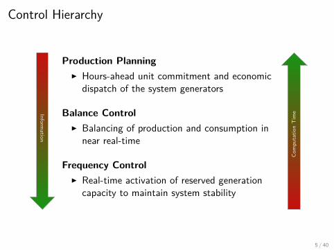
Control Hierarchy
Information
Production PlanningI Hours-ahead unit commitment and economic
dispatch of the system generators
Balance ControlI Balancing of production and consumption in
near real-time
Frequency ControlI Real-time activation of reserved generation
capacity to maintain system stability
Com
puta
tion
Tim
e
5 / 40

Case Study: The Faroe Islands
I Population of about 50,000people
I No interconnectors to othercountries (isolated power system)
I Some of the worlds bestconditions for wind power
I Target: 100% renewable energyby 2030
I Flexibility on both the productionand the consumption side ofenergy
Current challenges for the Faroe Islands are future challenges forlarger interconnected power systems
6 / 40

Key Contributions
I Proof of concept for balance and frequency EMPC-basedcontrol schemes
I Mean-Variance EMPC accounts for the inherent uncertaintyand variability of renewable energy sources
I Integrated planning and control using a hierarchical EMPCalgorithm
I Computationally efficient algorithms overcome tractabilityissues of the proposed EMPC schemes
I An optimal reserve planning problem for unit commitment andeconomic dispatch in small isolated power systems
7 / 40

Economic MPC of Energy Systems
8 / 40

Economic MPC (EMPC)
Optimal Control Problem
min.u,x ,z
φ (u, x , z)
s.t. xk+1 = Axk + Buk , k ∈ N0
zk = Czxk , k ∈ N1
(u, x , z) ∈ X
I Prediction horizon Ni = {0 + i , 1 + i , . . . ,N − 1 + i}
I Input vector u = (uT0 , uT
1 , uT2 , . . . , uT
N−1)T ∈ RNnu
I State vector x = (xT1 , xT
2 , xT3 , . . . , xT
N )T ∈ RNnx
I Output vector z = (zT1 , zT
2 , zT3 , . . . , zT
N )T ∈ RNnz
Assumption: Cost function φ is a convex function and constraintset X is a convex set
9 / 40
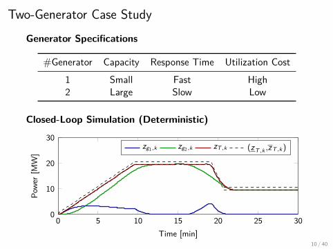
Two-Generator Case Study
Generator Specifications
#Generator Capacity Response Time Utilization Cost
1 Small Fast High2 Large Slow Low
Closed-Loop Simulation (Deterministic)
0 5 10 15 20 25 300
10
20
30
Time [min]
Powe
r[M
W]
zg1,k zg2,k zT ,k (zT ,k ,zT ,k )
10 / 40

Uncertainty Management
Closed-Loop Simulation (Stochastic)
0 5 10 15 20 25 300
10
20
30
Powe
r[M
W]
zg1,k zg2,k zT ,k (zT ,k ,zT ,k )
Certainty-Equivalent EMPC does not perform well in the presenceof uncertainty
11 / 40

Certainty-Equivalent EMPC (CE-EMPC)
I Linear stochastic system
xk+1 = Axk + Buk + wk , k ∈ N0
yk = Cy xk + vk , k ∈ N1
zk = Czxk , k ∈ N1
I Affine functions
x = Lx (u; x0,w)z = Lz(u; x0,w)
I Cost function
ψ(u; x0,w) = φ (u, Lx (u; x0,w), Lz(u; x0,w))
I Optimal control problemmin.u∈U
ΨCE = ψ(u; x0,E [w ])
12 / 40

Mean-Variance EMPC (MV-EMPC)
I CE-EMPC does not minimize the expected costψ(u; x0,E [w ]) 6= E [ψ(u; x0,w)]
670 680 690 700 710 720 7300
200
400
600
800
ψ(u∗CE ; x0,w)
Coun
ts
ψ(u∗CE ; x0,E [w ])
I MV-EMPCmin.u∈U
ΨMV = αE [ψ(u; x0,w)] + (1− α)V [ψ(u; x0,w)]
with risk-aversion parameter α ∈ [0; 1]13 / 40

Monte-Carlo Approximation
I Uncertainty scenarios S = {1, 2, . . . ,S}
I Optimal control problem
min.u∈U ,{x s ,zs ,ψs}s∈S ,µ
αµ+ 1−αS−1
∑s∈S
(ψs − µ)2 ,
s.t. x sk+1 = Ax s
k + Buk + w sk , k ∈ N0, s ∈ S
zsk = Czx s
k , k ∈ N1, s ∈ Sψs = φ(u, x s , zs), s ∈ Sµ = 1
S∑s∈S
ψs
I Two-stage extension with non-anticipative constraints can beapplied for less conservative closed-loop performance
I Large-scale optimization problem even for small systems14 / 40

Performance of MV-EMPC
0 5 10 15 20 25 30 35
210
220
230
240
α = 0α = 1
s
µ
MV-EMPCCE-EMPC
Computationally Attractive Alternatives
I Safety margin using constraint back-off
I Augmented objective function, e.g. setpoint-based penaltyterms and/or regularization terms
MV-EMPC provides a baseline for performance evaluation15 / 40

Frequency Control via EMPC
I Objective 1: Avoid critical frequency fluctuations
0 5 10 15 20 25 30 35 40
48
49
50
Time [sec]
Freq
uenc
y[H
z]
I Objective 2: Minimize cost of operations
16 / 40
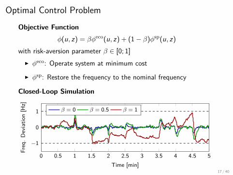
Optimal Control Problem
Objective Functionφ(u, z) = βφeco(u, z) + (1− β)φsp(u, z)
with risk-aversion parameter β ∈ [0; 1]I φeco: Operate system at minimum cost
I φsp: Restore the frequency to the nominal frequency
Closed-Loop Simulation
0 0.5 1 1.5 2 2.5 3 3.5 4 4.5 5
−1
0
1
Time [min]
Freq
.D
evia
tion
[Hz]
β = 0 β = 0.5 β = 1
17 / 40

Optimization Algorithms
18 / 40

Computational Aspects of EMPC
Problem structure is utilized for real-time solution of the OCPs
s1 s2 s3
(a) Scenario Coupling
g1 g2 g3
(b) Generator Coupling
t1 t2 t3
(c) Temporal Coupling
I Case (a) and (b) are handled by decomposition methods
I Case (c) is handled using Riccati-based methods
I Nested structures occur (c)→(b)→(a)
19 / 40

EMPC Decomposition Algorithms
Schematic Diagram
Aggregator (Master Problem)
Subproblem 1 Subproblem 2 Subproblem 3 Subproblem 4
Subproblems can be solved in parallel and warm-start is applicable
Methods
Method Problem Class Iterations Accuracy DimensionsDWD LPs Few High IncreasingADMM CPs Many Low Constant
20 / 40

Example: Block-Angular LPs
I Problem formulation
mint
{∑j∈J
cTj tj | Gjtj ≤ gj , j ∈ J ,
∑j∈J
Hjtj ≤ h}
I DWD: Extreme point representation
I ADMM: Problem splitting using auxiliary variables
vj = Hjtj , j ∈ J
Formulation of modified problem and simplified recursion ischallenging
21 / 40

Benchmark
CPU Time to Solve the OCP
101 102 103
10−1
10−2
100
101
102
No. of Generators
CPU
Tim
e[se
c]
DWempc ADMMempc GurobiCPLEX MOSEK
I Memory issue around M = 3000 for centralized solves
I The performance of ADMM is very problem dependent22 / 40

Further ADMM Results
MV-EMPC
Step Description
1 Solve a single OCP for each uncertainty scenario2 Minimize variance s.t. non-anticipative constraints
Input-Constrained EMPC
Step Description
1 Solve unconstrained OCP2 Solve input-constrained OCP with no dynamics
A speedup in computational speed of more than an order ofmagnitude is achieved for both cases
23 / 40

Homogeneous and Self-Dual Interior-Point Method
I Solution of the OCP minx{gT x |Ax = b, Cx ≤ d} is obtained
from solution of (z , s, τ, κ) ≥ 0 and
AT y + CT z + gτ = 0, Ax − bτ = 0Cx − dτ + s = 0, −gT x − bT y − dT z + κ = 0
I Warm-start works well for homogeneous and self-dual IPMs
tk Time
Inpu
t
u∗(k − 1) u∗(k)
I Search direction is computed using a Riccati-iterationprocedure
24 / 40

LP Solver Comparison
101 10210−2
10−1
100
101
102
103
104
No. of Generators
CPU
Tim
e[se
c]
LPempc
Gurobi
CPLEX
MOSEK
FORCES
101 10210−2
10−1
100
101
102
103
Horizon Length
Warm-start reduces the CPU time by further 40% on average25 / 40

Integrated Planning and Control
26 / 40

Production Planning
I Binary decisions b = (bT0 , bT
1 , . . . , bTL )T
I Problem formulation (simplified)min.
u,x ,z,bfR(u, x , z , b) + fZ(b)
s.t. xk+1 = Axk + Buk + Edk , k ∈ N0
zk = Czxk + Fzdk , k ∈ N1
cR(u, x , z , b) ≤ 0cZ(b) ≤ 0
I Two time scales
τ0 τ1 τ2 τL−1 τL
t0 t1 t2 t3 t4 tf−2 tf−1 tf
∆t
∆τ27 / 40

Hierarchical Algorithm
0 2 4 6 8 10 12 14 16 18 20
horizon of LL-OCP
Time [min]
Gene
rato
rSe
tpoi
nt[M
W]
UL-OCPLL-OCP
I The UL-OCP (MIQP/MILP) is closely related to the unitcommitment problem
I The UL-OCP may be solved with a low frequency
I Tailored algorithms can solve the LL-OCP (QP/LP) efficiently28 / 40

Three-Generator Example
0 20 40 60 80 100 120 140 160 1800
20
40
Time [min]
Powe
r[M
W]
r d d0 d900
I Direct solution of the full OCP is 15 minutes
I Solution times are 2s (UL-OCP) and 0.1s (LL-OCP)
I Single resolve of the UL-OCP is performed
I Cost increase is less than 1% for the hierarchical approach29 / 40

Optimal Reserve Planning
30 / 40
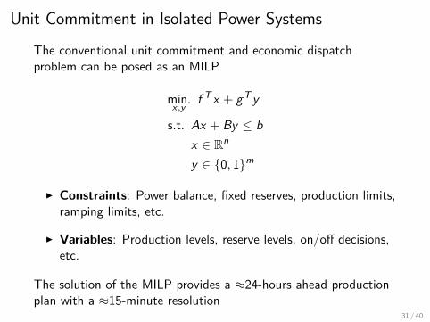
Unit Commitment in Isolated Power Systems
The conventional unit commitment and economic dispatchproblem can be posed as an MILP
min.x ,y
f T x + gT y
s.t. Ax + By ≤ bx ∈ Rn
y ∈ {0, 1}m
I Constraints: Power balance, fixed reserves, production limits,ramping limits, etc.
I Variables: Production levels, reserve levels, on/off decisions,etc.
The solution of the MILP provides a ≈24-hours ahead productionplan with a ≈15-minute resolution
31 / 40

Operational Reserves
t = 0
Post-contingentstate (stationary)
f ′(t) ≈ 1K ∆P(t) (ttr, f tr)
f nom
Pre-contingentstate
Post-contingentstate (transient)
Time [sec]
Freq
uenc
y[H
z]
I Primary reserves are critical to avoid power outages(blackouts) in the event of a contingency ∆P(t) 6= 0
I Primary reserves are activated in direct proportion to thefrequency deviation from the nominal frequency
32 / 40

Minimum Frequency Constraint
It is critical that f (t) ≥ f for some cut-off frequency f
I Large interconnected systemsSystem inertia is large and approximately constant⇒ A fixed amount of primary reserve is sufficient
I Small isolated power systemsSystem inertia is small and varies considerably⇒ Minimum frequency constraints are required
The constraint f (t) ≥ f is intractable to handle usingmixed-integer linear programming
33 / 40

Alternative Formulation
The minimum frequency constraint
f (t) ≥ f
may be expressed as
EPR(t) + ∆E rot ≥ P lostt
I EPR(t) =∫ t
0 PPR(τ)dτ is the energy contribution from theactivation of primary reserves
I ∆E rot is the energy contribution from the system inertia
I P lostt is the energy lost as a result of the contingency(generator trip)
34 / 40

Sufficient Conditions
I Minimum frequency occurs no later than time tc
PPR(tc) ≥ P lost
I Satisfy f (t) ≥ f for t ≤ tc, i.e.EPR(t) + ∆E rot ≥ P lostt, t ≤ tc
t = 0 t = tc
ff tr
Time [sec]
Freq
uenc
y[H
z]
35 / 40

Optimal Reserve Planning Problem (ORPP)
I Unit commitment and economic dispatch problem withminimum frequency constraints
I Compared to a conventional production and reserve planningproblem (BLUC)
I Simulations show that several potential blackouts are avoidedat a cost increase of 3%
I Tested in the Faroe Islands in 2015
36 / 40

Conclusions & Future Work
37 / 40

Conclusions
MethodsI MV-EMPC overcomes performance issues of CE-EMPC in
operation of uncertain systemsI MV-EMPC provides a baseline for approximate methods
AlgorithmsI Tailored decomposition schemes significantly reduces
computational requirements of the proposed EMPC methodsI Additional speedup is achieved using Riccati-based IPMs
ApplicationsI Simulations demonstrate that EMPC-based methods for
balance and frequency control reduce cost and riskI Unifying framework for balance control and unit commitmentI Frequency-constrained planning in isolated power systems
38 / 40

Future Work
Feedback From ExperimentsI Use feedback from the Faroe Islands to improve the proposed
planning and control methods
Risk Measures in MV-EMPCI Employ other risk measures than the varianceI Increase sensitive to the tail shape of the cost distributionI Develop algorithms to solve the resulting OCPs efficiently
Algorithms for EMPCI Quadratic programming extensions of LP solversI Tuned and parallel implementationsI Scenario reduction in MV-EMPC
39 / 40

Thanks! Questions and Comments?
40 / 40