Methods for analysis and control of dynamical systems ...o.sename/docs/AUTO_E7... · Case of PID controllers Lead compensation Lag compensation Matlab examples Methods for analysis

Control ofdynamicalsystems

O.Sename

Introduction

Concept

Rules

DynamiccompensationSpecifications

Case of PID controllers

Lead compensation

Lag compensation

Matlab examples

Methods for analysis and control ofdynamical systems

Lecture 4: The root locus design method

O. Sename1

1Gipsa-lab, CNRS-INPG, [email protected]

www.lag.ensieg.inpg.fr/sename

17th March 2010


O.Sename

Introduction

Concept

Rules



Lead compensation

Lag compensation

Matlab examples

Outline

Introduction

Concept

Rules

Dynamic compensationSpecificationsCase of PID controllersLead compensationLag compensation

Matlab examples


O.Sename

Introduction

Concept

Rules



Lead compensation

Lag compensation

Matlab examples

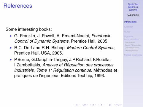
References

Some interesting books:I G. Franklin, J. Powell, A. Emami-Naeini, Feedback

Control of Dynamic Systems, Prentice Hall, 2005I R.C. Dorf and R.H. Bishop, Modern Control Systems,

Prentice Hall, USA, 2005.I P.Borne, G.Dauphin-Tanguy, J.P.Richard, F.Rotella,

I.Zambettakis, Analyse et Regulation des processusindustriels. Tome 1: Regulation continue, Methodes etpratiques de l’ingenieur, Editions Technip, 1993.


O.Sename

Introduction

Concept

Rules



Lead compensation

Lag compensation

Matlab examples

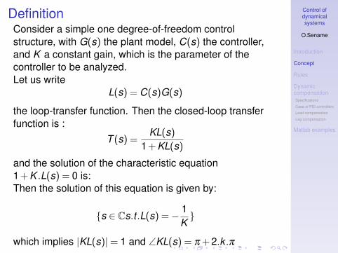
DefinitionConsider a simple one degree-of-freedom controlstructure, with G(s) the plant model, C(s) the controller,and K a constant gain, which is the parameter of thecontroller to be analyzed.Let us write

L(s) = C(s)G(s)

the loop-transfer function. Then the closed-loop transferfunction is :

T (s) =KL(s)

1+KL(s)

and the solution of the characteristic equation1+K .L(s) = 0 is:Then the solution of this equation is given by:

{s ∈ Cs.t .L(s) =− 1K}

which implies |KL(s)|= 1 and ∠KL(s) = π +2.k .π


O.Sename

Introduction

Concept

Rules



Lead compensation

Lag compensation

Matlab examples

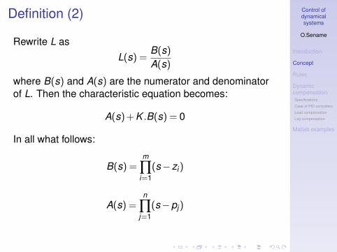
Definition (2)

Rewrite L asL(s) =

B(s)

A(s)

where B(s) and A(s) are the numerator and denominatorof L. Then the characteristic equation becomes:

A(s)+K .B(s) = 0

In all what follows:

B(s) =m

∏i=1

(s−zi)

A(s) =n

∏j=1

(s−pj)


O.Sename

Introduction

Concept

Rules



Lead compensation

Lag compensation

Matlab examples

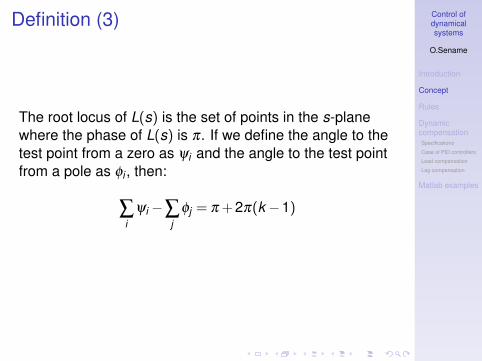
Definition (3)

The root locus of L(s) is the set of points in the s-planewhere the phase of L(s) is π. If we define the angle to thetest point from a zero as ψi and the angle to the test pointfrom a pole as φi , then:

∑i

ψi −∑j

φj = π +2π(k −1)


O.Sename

Introduction

Concept

Rules



Lead compensation

Lag compensation

Matlab examples

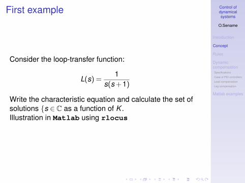
First example

Consider the loop-transfer function:

L(s) =1

s(s +1)

Write the characteristic equation and calculate the set ofsolutions {s ∈ C as a function of K .Illustration in Matlab using rlocus


O.Sename

Introduction

Concept

Rules



Lead compensation

Lag compensation

Matlab examples

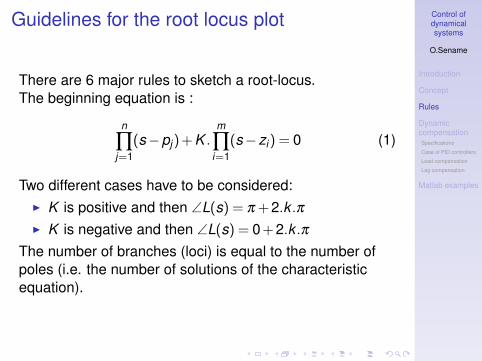
Guidelines for the root locus plot

There are 6 major rules to sketch a root-locus.The beginning equation is :

n

∏j=1

(s−pj)+K .m

∏i=1

(s−zi) = 0 (1)

Two different cases have to be considered:I K is positive and then ∠L(s) = π +2.k .π

I K is negative and then ∠L(s) = 0+2.k .π

The number of branches (loci) is equal to the number ofpoles (i.e. the number of solutions of the characteristicequation).


O.Sename

Introduction

Concept

Rules



Lead compensation

Lag compensation

Matlab examples

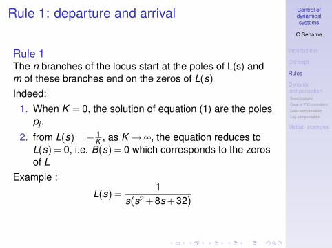
Rule 1: departure and arrival

Rule 1The n branches of the locus start at the poles of L(s) andm of these branches end on the zeros of L(s)

Indeed:1. When K = 0, the solution of equation (1) are the poles

pj .

2. from L(s) =− 1K , as K → ∞, the equation reduces to

L(s) = 0, i.e. B(s) = 0 which corresponds to the zerosof L

Example :

L(s) =1

s(s2 +8s +32)


O.Sename

Introduction

Concept

Rules



Lead compensation

Lag compensation

Matlab examples

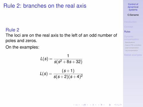
Rule 2: branches on the real axis

Rule 2The loci are on the real axis to the left of an odd number ofpoles and zeros.On the examples:

L(s) =1

s(s2 +8s +32)

L(s) =(s +1)

s(s +2)(s +4)2


O.Sename

Introduction

Concept

Rules



Lead compensation

Lag compensation

Matlab examples

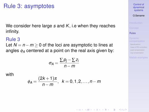
Rule 3: asymptotes

We consider here large s and K , i.e when they reachesinfinity.

Rule 3Let N = n−m ≥ 0 of the loci are asymptotic to lines atangles φA centered at a point on the real axis given by:

σA =∑pj −∑zi

n−m

withφA =

(2k +1)π

n−m, k = 0,1,2, . . . ,n−m


O.Sename

Introduction

Concept

Rules



Lead compensation

Lag compensation

Matlab examples

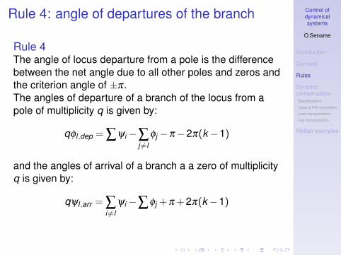
Rule 4: angle of departures of the branch

Rule 4The angle of locus departure from a pole is the differencebetween the net angle due to all other poles and zeros andthe criterion angle of ±π.The angles of departure of a branch of the locus from apole of multiplicity q is given by:

qφl ,dep = ∑ψi −∑j 6=l

φj −π−2π(k −1)

and the angles of arrival of a branch a a zero of multiplicityq is given by:

qψl ,arr = ∑i 6=l

ψi −∑φj +π +2π(k −1)


O.Sename

Introduction

Concept

Rules



Lead compensation

Lag compensation

Matlab examples

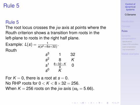
Rule 5

Rule 5The root locus crosses the jω axis at points where theRouth criterion shows a transition from roots in theleft-plane to roots in the right half plane.Example: L(s) = 1

s(s2+8s+32).

Rouths3 1 32s2 8 Ks1 8×32−K

8 0s0 K

For K = 0, there is a root at s = 0.No RHP roots for 0 < K < 8×32 = 256.When K = 256 roots on the jω axis (ωc = 5.66).


O.Sename

Introduction

Concept

Rules



Lead compensation

Lag compensation

Matlab examples

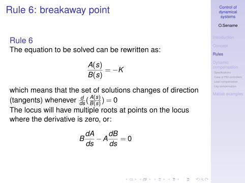
Rule 6: breakaway point

Rule 6The equation to be solved can be rewritten as:

A(s)

B(s)=−K

which means that the set of solutions changes of direction(tangents) whenever d

ds (A(s)B(s)) = 0

The locus will have multiple roots at points on the locuswhere the derivative is zero, or:

BdAds−A

dBds

= 0


O.Sename

Introduction

Concept

Rules



Lead compensation

Lag compensation

Matlab examples

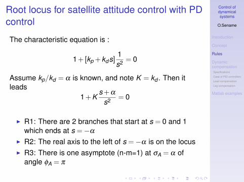
Root locus for satellite attitude control with PDcontrol

The characteristic equation is :

1+[kp +kds]1s2 = 0

Assume kp/kd = α is known, and note K = kd . Then itleads

1+Ks +α

s2 = 0

I R1: There are 2 branches that start at s = 0 and 1which ends at s =−α

I R2: The real axis to the left of s =−α is on the locusI R3: There is one asymptote (n-m=1) at σA = α of

angle φA = π


O.Sename

Introduction

Concept

Rules



Lead compensation

Lag compensation

Matlab examples

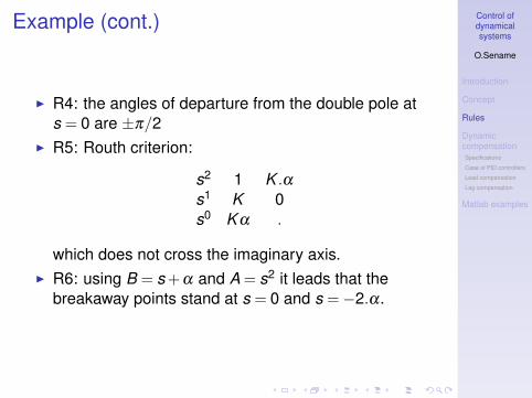
Example (cont.)

I R4: the angles of departure from the double pole ats = 0 are ±π/2

I R5: Routh criterion:

s2 1 K .α

s1 K 0s0 K α .

which does not cross the imaginary axis.I R6: using B = s +α and A = s2 it leads that the

breakaway points stand at s = 0 and s =−2.α.


O.Sename

Introduction

Concept

Rules



Lead compensation

Lag compensation

Matlab examples

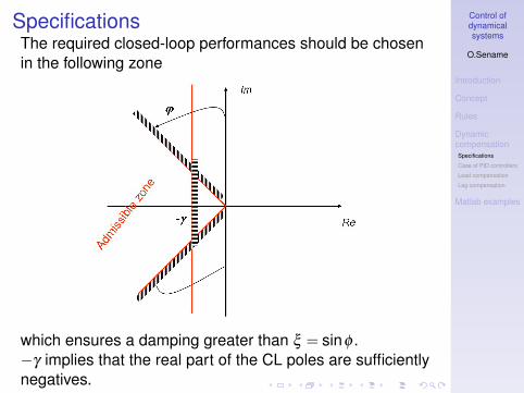
SpecificationsThe required closed-loop performances should be chosenin the following zone

which ensures a damping greater than ξ = sinφ .−γ implies that the real part of the CL poles are sufficientlynegatives.


O.Sename

Introduction

Concept

Rules



Lead compensation

Lag compensation

Matlab examples

Specifications (2)

Some useful rules for selection the desired pole/zerolocations (for a second order system):

I Rise time : tr ' 1.8ωn

I Seetling time : ts ' 4.6ξ ωn

I Overshoot Mp = exp(−πξ/sqrt(1−ξ 2)):ξ = 0.3⇔Mp = 35%,ξ = 0.5⇔Mp = 16%,ξ = 0.7⇔Mp = 5%.


O.Sename

Introduction

Concept

Rules



Lead compensation

Lag compensation

Matlab examples

PID controller

A PID controller is given by:

C(s) = Kp(1+1

Ti s+Td s) = Kp +KD s +

KI

s

For convenience it will be rewritten as :

C(s) = KD(s +z1)(s +z2)

s

which has one pole at the origine and two stable zeros.


O.Sename

Introduction

Concept

Rules



Lead compensation

Lag compensation

Matlab examples

Lead compensation

C(s) = K (s +zs +p

)

with z < p .

I Derivative-type controller : if p is placed well outsidethe frequency range of the design, the controller lookslike a PD controller.

I The effect of the zero is to move the locus to the left(towards more stable zones). To be chosen directlybelow the desired root location.

I p should be located left far on the real axis. It shouldensure that the total angle at the desired root locationis π


O.Sename

Introduction

Concept

Rules



Lead compensation

Lag compensation

Matlab examples

Lag compensation

C(s) = K (s +zs +p

)

with z > p.I Integration-type controller:I p should be closed to the origine. z sufficiently far.I z/p is chosen to be between 3 and 10 (according to

the need of boosting the steady-state gain).


O.Sename

Introduction

Concept

Rules



Lead compensation

Lag compensation

Matlab examples

Matlab example

Control of a small airplane (pitch attitude):

θ = G(s)(δ +Md)

where

G(s) =160(s +2.5)(s +0.7)

(s2 +5s +40)(s2 +0.03s +0.06)

θ is the pitch attitude, δ the elevator angle and Md thedisturbance moment .Specifications:

I rise time ≤ 1sec and overshoot less than 10%

I Design an autopilot so that the steady state value of δ

is zero for an arbitrary constant moment.


O.Sename

Introduction

Concept

Rules



Lead compensation

Lag compensation

Matlab examples

Matlab example

tr ≤ 1sec implies ωn ≥ 1.8.Mp ≤ 0.1 implies ξ ' 0.6.Steps

I Polynomial controllerI lead CompensationI Lead-lag compensation

Documents

Methods for analysis and control of dynamical systems ...o.sename/docs/AUTO_E7... · Case of PID controllers Lead compensation Lag compensation Matlab examples Methods for analysis