Embed Size (px)
Citation preview

StatPlan Consulting Pty Ltd
Methods for Assessment of the Conservation Status of Australian Inshore Dolphins Final report to Department of the Environment
Lyndon Brooks, Emma Carroll and Kenneth H. Pollock 29th May 2014

Methods for assessment of the conservation status of Australian inshore dolphins
1
Contents
Background ............................................................................................................................................. 4
EPBC Act Criteria ................................................................................................................................. 4
Objectives ........................................................................................................................................... 4
Objective 1: Extent of occurrence and area of occupancy of snubfin dolphins ..................................... 5
Background ......................................................................................................................................... 5
Extent of occurrence – current knowledge .................................................................................... 5
Orientation to methods .................................................................................................................. 6
Presence/absence and effort .......................................................................................................... 6
Home ranges, core habitat and mobility ........................................................................................ 6
Groups ............................................................................................................................................. 7
Sampling efficiency ......................................................................................................................... 7
General approach to sampling ............................................................................................................ 8
Primary sampling units ....................................................................................................................... 8
Size .................................................................................................................................................. 8
Location – Sites of type A (Estuarine sites) and B (Other sites) ...................................................... 9
Site accessibility and indigenous sea-ranger participation ........................................................... 11
Sites where large scale development is expected and marine parks ........................................... 12
Development of GIS ...................................................................................................................... 12
Secondary sampling units and sample zone types ........................................................................... 13
Zone types for sites of type A (Estuarine sites) ............................................................................. 14
Zone types for sites of type B (Other sites) .................................................................................. 14
Comments on sampling in secondary sampling units ................................................................... 14
Tertiary sampling units ..................................................................................................................... 15
Selecting sites for survey .................................................................................................................. 15
A sampling frame for sites of type A (Estuarine sites) .................................................................. 15
A sampling frame for sites of type B (Other sites) ........................................................................ 16
Defining sites ................................................................................................................................. 17
Methods for assessment of the conservation status of Australian inshore dolphins
2
Statistical models .............................................................................................................................. 18
Models based on collapsing level 3 units to level 2 units ............................................................. 18
A model based on omitting level 1 units ...................................................................................... 20
A model for data at 3 levels .......................................................................................................... 21
Comment on detection probability and density ........................................................................... 22
Covariates for sampling units ........................................................................................................... 22
Covariates for primary sampling units (level 1) ............................................................................ 22
Covariates for secondary sampling units (level 2) ........................................................................ 23
Covariates for tertiary sampling units (level 3) ............................................................................. 23
Sample size estimation ..................................................................................................................... 24
Observed group detection rates and the probability of detection given occupancy ................... 24
Partitioning the total number of surveys between sites (level 1) and surveys (level 2) .............. 25
Recommended sample size .......................................................................................................... 26
Discussion.......................................................................................................................................... 26
Considering the potential of aerial survey methods..................................................................... 26
Considering the potential of citizen science data ......................................................................... 27
Objective 2: Abundance in selected sites ............................................................................................. 28
Background ....................................................................................................................................... 28
Capture-recapture studies ................................................................................................................ 28
Population closure and temporary emigration for coastal dolphin populations ......................... 29
General principles for sampling intensity in the robust design .................................................... 30
Photo quality, the marked proportion and matching ................................................................... 32
Selection of sites for intensive study ................................................................................................ 33
Abundance, trends in abundance and threatening processes ..................................................... 33
Advantages to selecting sites for intensive monitoring from sites previously surveyed for
occupancy ..................................................................................................................................... 34
Transect design for capture-recapture studies ................................................................................. 35
A sample ........................................................................................................................................ 35
Methods for assessment of the conservation status of Australian inshore dolphins
3
Transect layout.............................................................................................................................. 35
Objective 3: Spatial and temporal risk assessment of current and projected threatening processes 36
References ............................................................................................................................................ 37
Appendix A – Simulation study ............................................................................................................. 40
Detection rates in level 2 units based on collapsing over level 3 units ............................................ 40
Expectations for psi (Ψ) .................................................................................................................... 41
Partitioning the total number of surveys between sites (level 1) and surveys (level 2) .................. 41
The simulation set ............................................................................................................................. 42
Summary ........................................................................................................................................... 44

Methods for assessment of the conservation status of Australian inshore dolphins
4
Background
This document recommends sampling and statistical methods for assessment of the conservation
status of inshore dolphins in line with the Australian Inshore Dolphin Research Framework
(Framework: Department of the Environment 2013a).
Following a review of the Environment Protection and Biodiversity Conservation Act 1999 (EPBC Act)
criteria, a prioritised list of objectives and actions to implement the Framework was composed at a
technical workshop on the research strategy held in Melbourne on 10th and 11th December 2012
(Department of the Environment 2013b). The results of this meeting have been incorporated in the
Framework.
While the research is focused on Australian snubfin dolphins (Orcaella heinsohni), data will also be
collected on humpback dolphins (Sousa chinensis) and bottlenose dolphins (Tursiops species).
EPBC Act Criteria
Criterion 3(B) was considered the most suitable as a guide for this research (see Appendix 1 of the
Framework) and ranked as the primary candidate with high priority, while Criteria 1 (A3) and 2 (B)
were considered of medium priority. Criterion 3 (B) requires an estimated total abundance of less
than 10,000 mature individuals, and evidence of continued decline and a precarious geographic
distribution.
Objectives
The objectives for the project as specified in the Framework (pp. 3-4) are:
“Objective 1. To conduct a broad-scale assessment of the extent of occurrence and area of
occupancy of snubfin dolphins. This should include: a compilation of existing data sources; the
development of an indigenous engagement and knowledge sharing strategy; the development of a
temporally and spatially replicated presence/absence boat surveys covering a large geographic
range.”
“Objective 2. To conduct dedicated multi-year studies of the distribution, abundance and habitat use
of snubfin dolphins at selected sites across northern Australia with differing levels of threatening
processes. The studies would provide a plausible estimate of rate of change within sites and by
extension, across the entire range.”
“Objective 3. To undertake a spatial and temporal risk assessment of current and projected
threatening processes that impact snubfin dolphins.”
Methods for assessment of the conservation status of Australian inshore dolphins
5
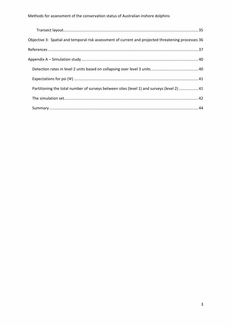
Collaboration was sought from a group of experienced inshore dolphin researchers and other
interested parties (Australian Inshore Dolphin Methods Working Group, AIDMWG) through an
electronic discussion process. This was to ensure that the sampling and statistical methods being
developed were viable in the field, consistent with existing knowledge and adequate to meet the
objectives of the Framework. Substantial feedback was received on several elements of the
proposed design.
Objective 1: Extent of occurrence and area of occupancy of snubfin
dolphins
Background
The Inshore Dolphin Research Framework summarises the current state of knowledge on snubfin
dolphins in the following terms:
“Australian snubfin dolphins (Orcaella heinsohni; hereafter snubfin dolphin) are found throughout
coastal waters of northern Australia. They live in small populations of approximately 50-100
individuals, inhabit shallow inshore and estuarine waters, exhibit fine-scale population structure and
have relatively small home ranges (Framework p.3).”
Snubfin dolphins appear to exist as a metapopulation with unknown levels of interaction between
sub-populations, some of which exhibit genetic differentiation over relatively short distances
(Framework pp. 6, 7).
Extent of occurrence – current knowledge
Current knowledge (Beasley et al. 2012) indicates that, apart from occasional vagrants, the extent of
occurrence of snubfin dolphins is limited to:
East coast southerly limit = Port Alma, QLD (-23.555625)
West coast southerly limit = Exmouth Gulf, Northwest Cape, WA (-21.791397)
Distance from land ≤ 20 km (including around islands < 35 km from mainland coast)
Water depth ≤ 20m
There is some evidence that, within this area, most snubfin dolphins are found within 20 km of a
river mouth and may frequently be found in estuarine areas (Parra et al. 2002, 2006). This may
reflect that most existing studies were located in such areas and that little information is available
from areas further from rivers.

Methods for assessment of the conservation status of Australian inshore dolphins
6
Orientation to methods
The geographic scale of the range of the species, the remoteness of much of the area, and that it
may include as few as 10,000 mature individuals overall, represent constraints on the sampling
design. In particular, the design needs to accommodate the expected low density and patchy
distribution of the species, and the relative accessibility of sites, including the cost of returning to re-
sample them. Additionally, that an argument for classification as vulnerable or endangered under
the EPBC Act will need to integrate information on distribution, abundance and threatening
processes requires that the methods proposed to meet each of the three objectives be optimally
compatible.
Presence/absence and effort
Objective 1 calls for presence/absence boat surveys. Strictly, when detection is imperfect,
‘presence/absence’ data can only be interpreted as detection/non-detection data because, while
detection indicates presence, non-detection cannot be taken to indicate absence. Statistical
methods that use repeat surveys to provide information on detection probability and tease apart the
occupancy and detection processes are required to estimate the proportion of sites that are
occupied (MacKenzie et al. 2006).
In addition to sampling with suitable replication to separate occupancy from detection, a reliable
measure of sampling effort is required to obtain data that are comparable between samples where
dolphins were and were not found and between survey sites.
Home ranges, core habitat and mobility
Current knowledge indicates that snubfin sub-populations occupy relatively small home ranges that
may often extend over less than 50 km of coastline (Cagnazzi et al. 2013). Sample sites defined over
stretches of coast of about this size will overlap with home ranges to varying degrees depending on
whether sub-populations are present in the areas, the locations of the cores (centroids) of their
activities (core habitat) relative to the locations of the sites, and the actual home range sizes of local
sub-populations.
We assume that, if a local population exists in the area, there is a non-zero probability of detecting
the species on survey within a site defined over 40-50 km of coast. The probability of detection will
vary with survey effort, sighting conditions and the density of the species on the survey site. The
density of the species on a survey site will in turn depend on the size of a local sub-population and
the extent of overlap between its home range and the survey area.

Methods for assessment of the conservation status of Australian inshore dolphins
7
We are not aware of any reason to suppose that sub-groups of animals in a local population
preferentially use different parts of its home range. Consequently, it’s reasonable to assume that
samples taken in different areas within the same 40-50 km of coast are random.
Groups
Snubfin, humpback and bottlenose dolphins typically travel in groups of varying sizes (1-20, mean =
approximately 5: Parra et al. 2002; Cagnazzi et al. 2013) and a presence/absence study will aim to
detect groups rather than individuals. Obviously, such groups need to be identified to species but,
because the EPBC Act Criteria are framed in terms of numbers of mature individuals, data are
required on group sizes so that information on the abundance (or sighting rates) of groups can be re-
expressed as the abundance (or sighting rates) of individuals. Information about fecundity is
inherent in counts of calves within groups and we recommend that these data be estimated in the
field along with group size.
Sampling efficiency
Many parts of the species’ range are remote and expensive to survey, and returning to re-sample
very remote sites would add greatly to the cost of the project. While replication is required to
separate the probability of occupancy (ψ) and the probability of detection in occupied sites (p|ψ),
replication may be achieved during a single survey session extending over a relatively short period
(days), or spatially rather than temporally by selecting spatial sub-samples within sites (Nichols et al.
2008; Kendall & White 2009; Guillera-Arroita 2011). With spatial replication detection is a
combination of the probability of dolphins being present in a sub-sample at the time of survey and
the probability that that they are detected if present.
A purely spatial approach to replication implies a one-off, cross-sectional survey that would not
permit modelling the influence of temporally variable factors on a site-by-site basis. Information on
this would be inherent, however, in across-site variation in the conditions prevailing at the time each
site was surveyed. Replicate surveys on the same site would be taken over several days however,
permitting modelling of the influence of factors that may vary over relatively short time spans.
Further insight into temporal effects could be obtained from data on a sub-set of sites selected for
intensive study under Objective 2 of the Framework. Temporally variable factors are unlikely to
greatly affect estimates of occupancy for sites defined on the approximate scale of a sub-population
home range although they may influence the rates of use of different habitat types within a site.
On-water boat-time is expensive and it is desirable that as much as possible is spent ‘on-effort’ and
as little as possible spent ‘off-effort’ travelling between transect segments. This requires that within-
Methods for assessment of the conservation status of Australian inshore dolphins
8
day sets of transect segments be contiguous and that such non-independence between detections
on adjacent segments as exists be accounted for statistically if necessary. An occupancy model for
this was described by Hines et al. (2010).
General approach to sampling
We recommended a general approach to sampling with 3 nested levels of sampling units:
1. Primary sampling units. Approximately home range sized primary sampling units (sites) of
40-50 km of coast plus inshore, sheltered area > 100 km2.
2. Secondary sampling units. Sets of contiguous 10km long transect segments within sites.
These units are independent replicates of the primary sampling units (sites). Each is as long
(includes as many segments) as can be sampled in a day.
3. Tertiary sampling units. Individual 10 km long transect segments. These units are serially
dependent replicates of the level 2 units.
While the secondary sampling units may be considered to be spatial replicates of sites because their
within-site locations will vary, they will generally be sampled on different days and may also be
considered to be temporal replicates.
Primary sampling units
Size
We recommend that areas of approximately the expected size of a sub-population home range be
selected as the primary sampling units for this research. In this situation, if such an area is occupied,
it is reasonable to expect that members of the local sub-population will be present there at all times.
Consequently, an estimate of the probability of occupancy of primary sampling units defined on the
approximately home range sized scale may be interpreted as an estimate of the probability of
residency. Smaller areas within a home range will be used with some frequency but may not be
continuously occupied, and estimates of occupancy at this level should be interpreted as indicating
rates of use rather than residency.
It is not necessary that all primary sampling units be the same size, although operationally it is
recommended that their sizes be similar. For primary sampling units of varying sizes, it is necessary
that each unit is spatially defined and its area calculated.
While current knowledge limits the extent of occurrence of snubfin dolphins to within 20 km from
land (Beasley et al. 2012), we recommend that sampling not be undertaken further than 10 km from
land in the interests of the safety of crews operating small boats and to minimise travel time to and

Methods for assessment of the conservation status of Australian inshore dolphins
9
from sampling sites. We assume that dolphins that may use areas between 10 and 20 km from land
will also use (and probably more often use) adjacent areas within 10 km from land. If part of a local
sub-population is more than 10 km from land at the time of sampling, we expect this to reduce the
probability of detection but not substantially affect the probability of occupancy.
Note that we do not employ water depth as a basis for defining primary sampling units. As
subsequently described, we recommend that depth be measured on transect (or derived from
bathymetry maps), for use as a covariate.
In sum, primary sampling units will typically extend over approximately 40-50 km of coast and out to
10 km from land, although their areas will vary depending upon the areas of within river (or inshore
sheltered area) included.
While the proposal to define sites on the approximate scale of sub-population home ranges, there is
little information on their actual sizes and they may be highly variable. Consequently, it should not
be assumed that an estimate of occupancy will provide a reliable basis for estimating the number of
sub-populations. It is possible that such areas could include members of more than one sub-
population and likely that some sub-populations range over areas that are larger than the survey
sites. The main objective of specifying sites on the suggested scale is to increase the probability that,
if such an area were occupied, members of the local sub-population would be present and available
for detection in the area at all times.
Location – Sites of type A (Estuarine sites) and B (Other sites)
The search area lies between Exmouth Gulf, Northwest Cape, WA and Port Alma, Queensland on the
mainland, includes islands up to 35 km from the mainland, and extends up to 10 km from land.
Ideally, each primary sampling unit would be centred on a point of expected focal habitat (centroid
of use) within a site. There is little information about snubfin habitat selection (Framework pp.6-7)
however, and it will be necessary select potentially arbitrary points on the coast to act as centres of
primary sampling units.
Rivers
While definitive information on the species’ preference for areas near river mouths is lacking across
the range, there is evidence for this on the coast of Queensland (Parra et al. 2002, 2006). The
locations of the mouths of major and minor rivers (e.g., Geofabric V2 data from Geofabric FTP site;
http://www.ga.gov.au/topographic-mapping/national-surface-water-information.html) also offer a
basis for identifying points around which primary sampling units (sites) can be defined.

Methods for assessment of the conservation status of Australian inshore dolphins
10
We recommend identification of river mouths to serve as focal points for defining most primary
sampling units, and that two broad site types are defined as follows:
A. Sites of type A. Estuarine sites. Major rives/Estuaries/Large, sheltered bays/Ports/Harbours.
Sites centred on the mouths of major rivers (and some additional focal points of comparable
sites, such as large sheltered bays, as described below) with at least 100 km2 of navigable
inshore, sheltered area.
B. Sites of type B. Other sites.
We recommend that large, sheltered bays, including harbours, be included among sites of type A. An
example of a large, sheltered bay that supports a relatively large population of snubfin dolphins, and
shares many of the features of a major river or estuary but without substantial freshwater inflow, is
Port Essington located on the Cobourg Peninsula, NT ( -11.256 , 132.150) (Palmer et al. 2014). A
rationale for inclusion of these sorts of areas among sites of type A is that they may provide
preferred, sheltered habitat for dolphins, and may also be attractive as sites for port or other coastal
development.
That estuaries and large sheltered bays are preferred habitat for snubfin dolphins represents a
hypothesis of interest when such sites are prime candidates for coastal development.
While adjacency to a river mouth is not a criterion for sites of type B, minor rivers are widely
distributed around the coast and their locations might be employed as a basis for composing a list of
potential points around which to define these sites. Only a small length of coast is greater than 50
km from the mouth of any river, large or small and exclusion of this area from the site selection
process is unlikely to introduce systematic bias in the estimated probability of occupancy.
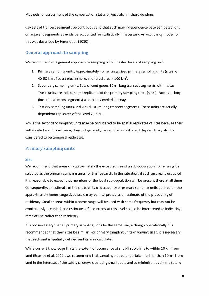
The terminus points (mouths) of major and minor rivers around the coast within the search area are
plotted in Figure 1. This plot was generated from a GIS constructed as an initial focus for the project
(Alana Grech). A subset of the list of major rivers from the GIS consisting of those that include at
least 100 km2 of inshore, sheltered area (essentially, an area of adequate size to contain at least 40
km of transect), supplemented with suitable bays and harbours, may be used to compose a sampling
frame for sites of type A.
A sampling frame for sites of type B might be composed by listing major rivers that do not meet the
inshore, sheltered area criterion for sites of type A together with the list of minor rivers, perhaps
supplemented with a subset of other arbitrary locations.
Methods for assessment of the conservation status of Australian inshore dolphins
11
Figure 1: Locations of mouths of major and minor rivers within the known snubfin range
Identification and definition of individual sites will need to be made following a fine-scaled
investigation of the coastline using the site-type category descriptions above as a guide. An estimate
of the total areas of sites of types A and B will be required for expansion of model estimates of the
probabilities of occupancy of these site types to estimate the total area of occupancy of the species.
One approach to this would be to create buffers around the sites in the two lists that extend 20-25
km either side of their focal points. While it may be difficult to calculate the total area of sites of
type A precisely as within-river areas are seasonally and tidally variable, and do not seem to be
systematically mapped, some basis needs to be devised for reasonable estimation of the total area
of the site types.
Site accessibility and indigenous sea-ranger participation
We considered construction of an accessibility-weighted sampling frame to try to maximise the
average accessibility of sample sites and to maximise the potential for participation by indigenous
sea-ranger groups. Investigation of roads to the coast identified very large sections that were
inaccessible by this means and we judged that it the credibility of an estimate of the probability of
occupancy over the whole range would be compromised by excluding these areas from sampling.

Methods for assessment of the conservation status of Australian inshore dolphins
12
While it was intended that, as far as possible, sampling work would be conducted from small, land
based vessels, an implication of including sites in the sampling frame that are inaccessible by road is
that a proportion of the sites selected for sampling would need to be accessed by larger vessels that
could safely travel there by sea. This may not be required for very many sites however, as a
reasonably large proportion of sites of type A may be accessible by road, although the proportion
may be lower for sites of type B.
We recommend that the minimum required number of sites of each site type (see Sample size
estimation below) be randomly selected from the sampling frame and that sea-ranger sites that
were not included be added.
This would mean that a suitably sized sample would be randomly selected and inference could be
based on that sample in the event that adding the non-randomly selected sites (e.g., sea-ranger
sites) substantially changed the estimated probability of occupancy.
A map of the locations of sea-ranger groups may be found here:
(http://www.environment.gov.au/indigenous/workingoncountry/projects/pubs/woc-projects-
map.pdf).
Sites where large scale development is expected and marine parks
Monitoring programs for large-scale developments are often commissioned too late for a pilot study
to be completed or for an accurate baseline assessment to be made. If sites where large-scale
developments are expected are included in the sample, the data collected there would constitute a
valuable pilot study for the design of subsequent capture-recapture monitoring programs. If such
sites can be identified they might be added to the sample as suggested above for inclusion of
indigenous sea-ranger sites.
It should be obvious that data from a preliminary survey for occupancy, while useful in designing a
capture-recapture study, would not provide a baseline estimate of abundance.
Selection of paired, potentially ‘impacted’ and ‘non-impacted’ sites is recommended for intensive
monitoring of a subset of sites (see Objective 2). Marine parks may be good candidates for ‘non-
impacted’ sites and might be paired with comparable ‘impacted’ sites for inclusion in the sample.
Development of GIS
More work is required to further develop the GIS to ensure consistency in identification of sites and
to maintain as much clarity to the distinction between site of types A and B as possible. Preliminary
investigation of the suggested approach has been examined in the Northern Territory and less
Methods for assessment of the conservation status of Australian inshore dolphins
13
intensively in WA, and while the approach is viable, further specification is recommended. A
systematic process of spatial definition of the site types is necessary for calculation of the total areas
of each type for expansion of the occupancy estimates up to an estimate of the total area of
occupancy. This is to emphasise that sites need to be selected from a sampling frame built on clear
decision rules prior to sample selection so that it is possible to identify sites that meet the rules but
were not surveyed so that estimates from those that were surveyed can be applied across the range.
Secondary sampling units and sample zone types
We recommend that zone types be defined within the primary sample sites and that the sets of
contiguous 10 km transect lengths composing secondary units be located within them. This is to
provide spatial and environmental coherence to each set of transect segments and to ensure
reasonable coverage of primary units.
It is necessary to define these zone types somewhat differently for primary sample sites of the
different types because primary sample sites of type A include substantial areas of inshore, sheltered
environment by definition, while sites of type B do not.
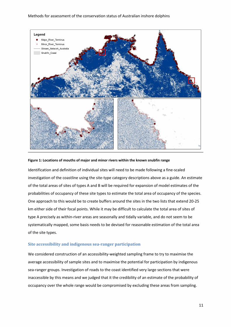
We initially defined two lines parallel to land at 5 km and 10 km from land. These lines are plotted in
Figure 2.
Figure 2: Lines representing distances of 5 km and 10 km from land
Methods for assessment of the conservation status of Australian inshore dolphins
14
Zone types for each site type are now elaborated using these lines as a basis and unifying factor.
Zone types for sites of type A (Estuarine sites)
Three zone types for sites of type A are defined in reference to the two distance from land lines and
a virtual line across the river mouth or the ‘mouth line’ (a line demarcating the inshore, sheltered
area from the oceanic environment):
1. Seaward from and within 5 km of the mouth line
2. Seaward from and between 5 and 10 km of the mouth line
3. The navigable, sheltered inshore zone (inside mouth line)
Zone types for sites of type B (Other sites)
Generally only two zones types are defined for sites of type B:
1. Within 5 km from land
2. Between 5 and 10 km from land
Comments on sampling in secondary sampling units
The total length of transect composing a secondary sampling unit will depend upon the total length
of transect that can be surveyed in a day. Anticipating subsequent discussion of sighting rates and
sample size estimation, 40 km should be considered to be a minimum target length of transect for
survey on a secondary sampling unit. This is because it may be necessary to aggregate over tertiary
sampling units to achieve a suitable detection rate for modelling. While secondary sampling unit
transect lengths of less than 40 km could occasionally be accommodated, longer lengths would
contribute to a more powerful analysis. In general, the length of transect that can be surveyed in a
day will depend upon the weather conditions, the distance of the first and last segments from ‘home
base’, and the efficiency of the crew.
This latter will depend at least partly upon what information the crew is sampling for apart from
group sightings and estimates of group size. The distribution study (Objective 1) does not require
information on individual dolphins, either photo-id or biopsy data.
If data from sets of tertiary sampling units are aggregated to single measures for secondary sampling
units, the principal data to be collected on a survey of a secondary sampling unit is whether at least
one group was detected or not. While covariate data and information on each sighting would also be
collected and used in modelling, only the presence or absence of at least one group is required for
the response variable. The shape of the set of transect line segments that constitute a survey of a
level 2 unit may vary: they could form a straight line, follow a zig-zag pattern, or compose a curve or
a loop. In terms of sampling efficiency, any pattern of transect line that maximises its length is
Methods for assessment of the conservation status of Australian inshore dolphins
15
appropriate. Zig-zag transects may be the most effective way to increase the length of transect in
the zone, and a loop may be of value in avoiding off-effort boat time when travelling up and back a
river, or in order to return to home base.
When sightings beyond the first in a set of transect segments are to be collapsed into a single
presence-absence point for analysis, it is not important that resights of the same group be avoided
or identified for the main occupancy study. This is important however, if the transect segment data
are to be used in analysis (see statistical models below) or counts are to be employed in a Royle
(2004) type of model, and some effort should be directed to identifying groups under circumstances
in which repeated sightings of the same groups are possible, perhaps by the features of one
distinctively-marked individual, or group size and composition. We recommend, therefore, that
effort be made to avoid or detect resights when they occur so that more informative models can be
fitted should they be justified by the data obtained.
Tertiary sampling units
Each level 3 unit is a length of transect, a contiguous set of which defines a level 2 unit and is
consequently located in a zone type. We recommend that a standard length be specified for these
units and have chosen 10 km on the assumption that, typically, between 4 and 8 could be surveyed
in a day, and in order to use this length as a basic, standard measure of effort.
Selecting sites for survey
A sampling frame for sites of type A (Estuarine sites)
A sampling frame for sites of type A could be constructed by beginning with a list of major rivers
within the search range. A list of large, sheltered bays, ports and harbours would be appended to the
list of major rivers to make a list of potential sites of type A. Each site on the list of potential sites of
type A would be assessed to determine whether it meets the criterion of at least 100 km2 of inshore,
sheltered area (or it’s possible to include at least 40 km of transect in the inshore, sheltered zone).
The sampling frame for sites of type A is the subset of the list of potential sites of type A that meet
the minimum inshore, sheltered water zone criterion.
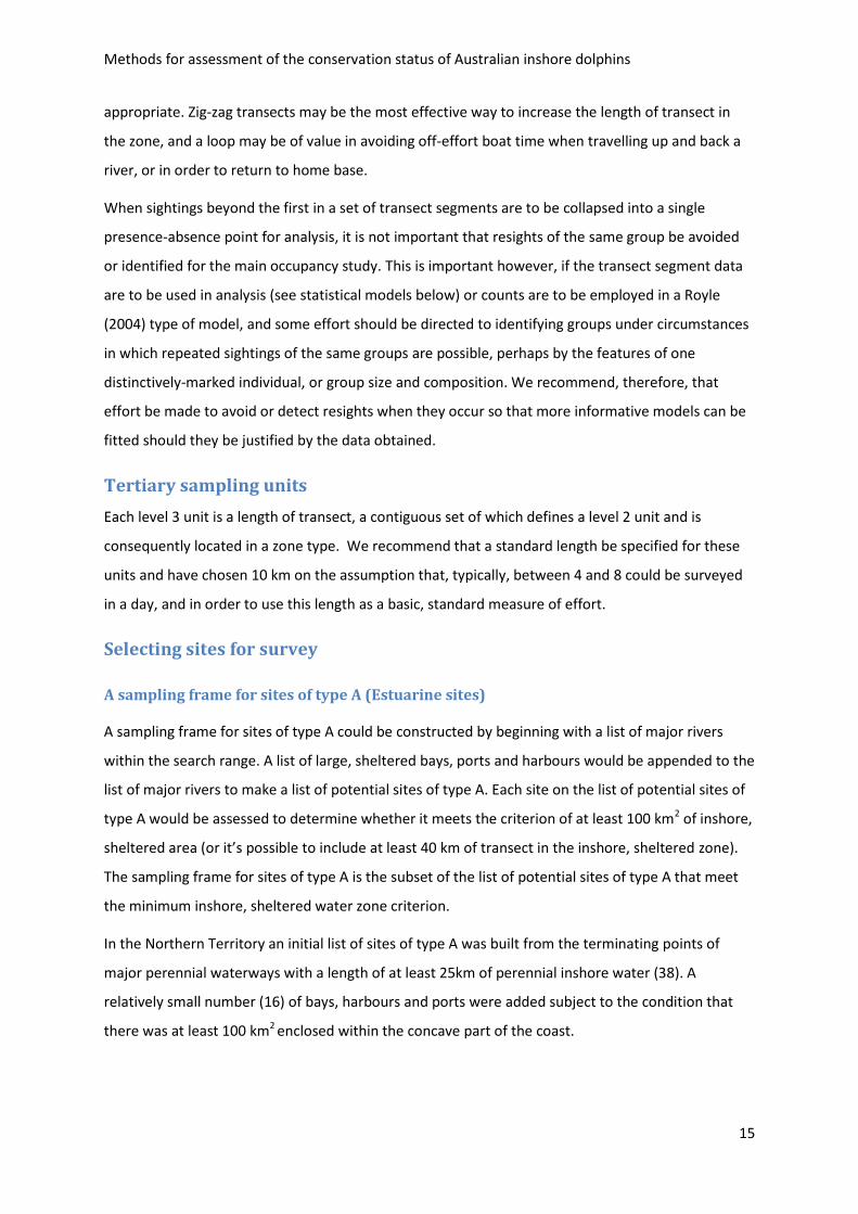
In the Northern Territory an initial list of sites of type A was built from the terminating points of
major perennial waterways with a length of at least 25km of perennial inshore water (38). A
relatively small number (16) of bays, harbours and ports were added subject to the condition that
there was at least 100 km2 enclosed within the concave part of the coast.
Methods for assessment of the conservation status of Australian inshore dolphins
16
Selection from the sampling frame for sites of type A
The sampling frame for sites of type A is sorted into random order. The first site on the ordered list is
chosen for sampling. The next site on the ordered list is chosen subject to the condition that its focal
point is not closer than 80 km from the focal point of the previously selected site, otherwise the next
site is chosen from the ordered list. The process is continued until the target number of sites of type
A is selected.
The minimum distance criterion is calculated on an ‘as the dolphin swims’ basis.
In the Northern Territory the list of potential sites of type A was sorted into random order and the
first selected for sampling. The next and subsequent sites were selected in order subject to the
condition that no site of type A was within 80 km of any other site of type A until 20 sites were
identified.
A sampling frame for sites of type B (Other sites)
A sampling frame for sites of type B could be constructed by beginning with a list of minor rivers
within the search range (this is a large list). The list of potential sites of type A that did not meet the
minimum sheltered water criterion would be appended to the list of minor rivers to make the
sampling frame for sites of type B.
In the Northern Territory an initial list of sites of type B was built from a list of the terminating points
of minor waterways (1108) supplemented with major perennial waterways that did not meet the
criteria for a site of type A (13).
Selection from the sampling frame for sites of type B
The sampling frame for sites of type B is sorted into random order. The first site on the ordered list is
chosen for sampling, subject to the condition that its focal point is not closer than 55 km from the
focal point of a site of type A. The next site on the ordered list is chosen subject to the condition that
its focal point is not closer than 55 km from the focal point of any previously selected site of either
type A or type B, otherwise the next site is chosen from the ordered list. The process is continued
until the target number of sites of type B is selected.
In the Northern Territory the list of potential sites of type B was sorted into random order and the
first selected for sampling subject to the condition that it was not closer than 55 km from a site of
type A. The next and subsequent sites were selected in order subject to the condition that no site
was within 55 km of any other site until 20 sites were identified.
Methods for assessment of the conservation status of Australian inshore dolphins
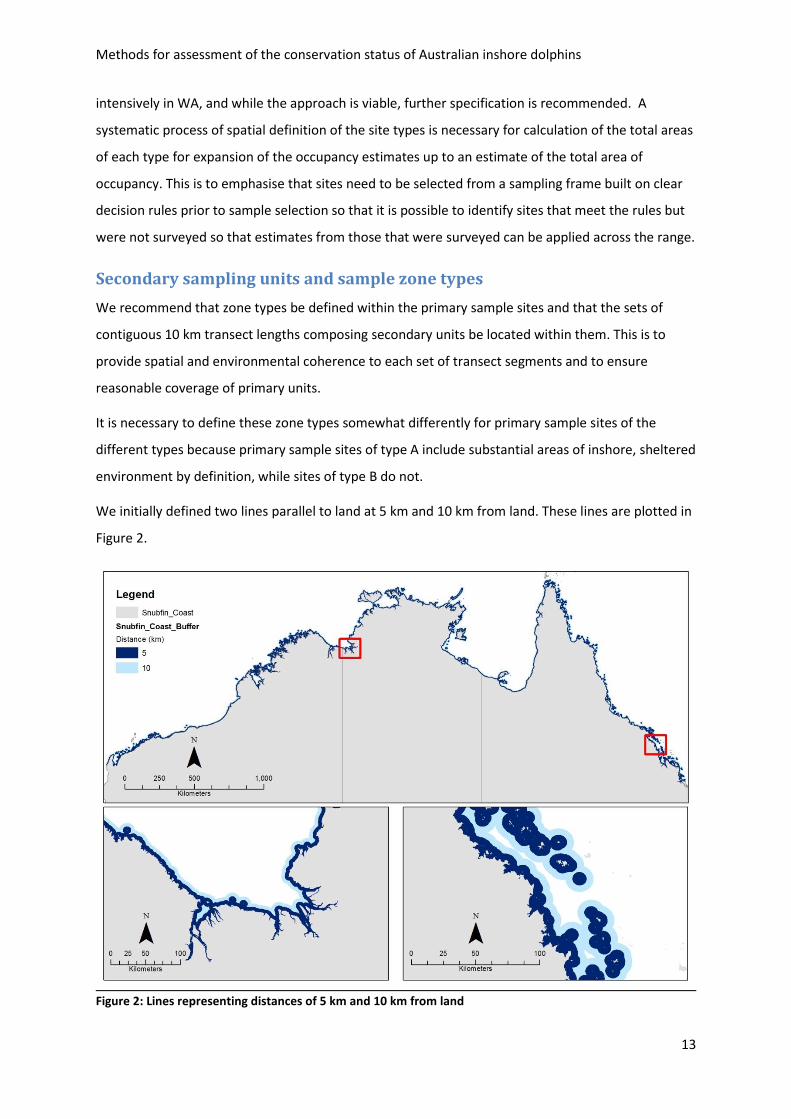
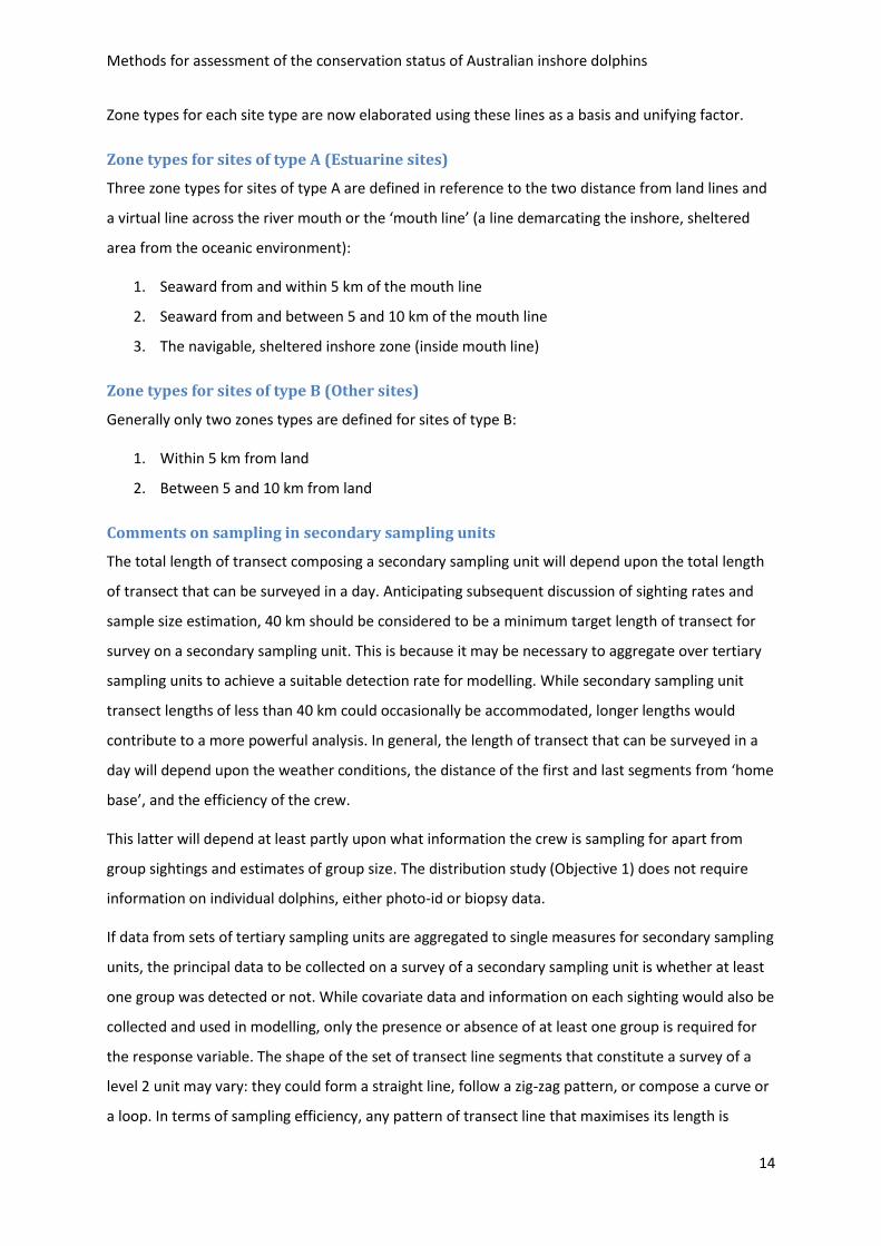
17
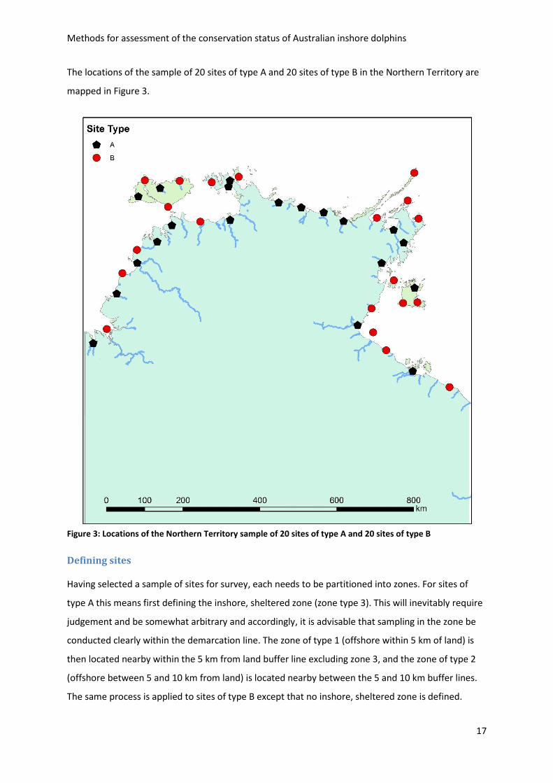
The locations of the sample of 20 sites of type A and 20 sites of type B in the Northern Territory are
mapped in Figure 3.
Figure 3: Locations of the Northern Territory sample of 20 sites of type A and 20 sites of type B
Defining sites
Having selected a sample of sites for survey, each needs to be partitioned into zones. For sites of
type A this means first defining the inshore, sheltered zone (zone type 3). This will inevitably require
judgement and be somewhat arbitrary and accordingly, it is advisable that sampling in the zone be
conducted clearly within the demarcation line. The zone of type 1 (offshore within 5 km of land) is
then located nearby within the 5 km from land buffer line excluding zone 3, and the zone of type 2
(offshore between 5 and 10 km from land) is located nearby between the 5 and 10 km buffer lines.
The same process is applied to sites of type B except that no inshore, sheltered zone is defined.

Methods for assessment of the conservation status of Australian inshore dolphins
18
Occasionally, in some sites, one or more of the zones will not be continuous in space and may
consist of two or more areas, this would occur for example when the 5 km from shore line intersects
the mouth line. The total area of each site and the areas of each of the zones within the sites should
be recorded.
Statistical models
The book by MacKenzie et al. (2006) is the core general reference for occupancy modelling. The
development of occupancy models has been rapid since publication of the paper MacKenzie et al.
(2002). Occupancy models may be fitted in the software programs Presence (http://www.mbr-
pwrc.usgs.gov/software/presence.shtml) and Mark (http://www.phidot.org/software/mark/).
While we have recommended a 3-level sampling structure, two-level data may be derived under
either of two scenarios:
1. Scenario 1 - collapsing over the level 3 units (transect segments) within each level 2 unit for
a model using levels 1 (sites) and 2 (replicates or surveys), or
2. Scenario 2 - omitting the level 1 units and using levels 2 (zone-type samples) and 3 (transect
segments) and constructing a spatial dependence model to accommodate the non-
independence in the series of contiguous transect segments (Hines et al. 2010) under an
approach that accommodates the clustering of level 2 units within level 1 units (sites).
One implication of aggregating over level 3 units (transect segments) to compose level 2 units is the
loss of within-day variation in environmental characters and detection covariates. Location of level 2
samples in zone types should ensure that covariate values are reasonably consistent within samples
and that mean values provide reasonable measures for the units as wholes. Although unlikely to be
employed directly in analysis, the transect segment level 3 units remain useful as providing a
consistent measure of effort and a basis for measurement of covariates. Alternative models that
employ the level 3 data directly were briefly described above for the event that detection rates are
greater than anticipated, as they may be for humpback or possibly bottlenose dolphins.
Models based on collapsing level 3 units to level 2 units
Here we describe three, two-level models based on Scenario 1 (collapsing level 3 data to level 2):
A standard ‘single season’ occupancy model for data at levels 1 (site) and 2 (replicates, or
surveys) (MacKenzie et al. 2002) – the recommended model
A single season occupancy model for more than one species (MacKenzie et al. 2004)
A N-Mixture model for abundance in which the derived level 2 data are binomial counts
rather than presence/absence (Royle 2004)
Methods for assessment of the conservation status of Australian inshore dolphins
19
The standard two-level (single season) occupancy model
For models fitted to data derived by collapsing over the level 3 units (transect segments) within each
level 2 unit, occupancy estimates apply to the primary sampling units of which level 2 units are
replicates.
These are highly mobile animals that are expected to range widely within their home ranges; we also
expect groups to be distributed widely throughout the site at any time, although there may be a
general pattern of movement with tides or other factors. To apply this model, we assume that, while
rates of use of the zone types may vary, there is a non-zero probability of their detection in all zones
during the course of any day, or in any zone on the day it is sampled. The appropriate model in this
case is a standard single season occupancy model (MacKenzie et al. 2006; see Kendall & White 2009
and Guillera-Arroita 2011 for considerations relating to spatial rather than temporal replication).
The parameters of the model are
{ , },
probability of occupancy of sites, and
probability of detection given site is occupied
p
where
p
In fitting this model, zone type would be assessed as a covariate on detection probability p to adjust
for variation in rates of use among zone-types, along with the mean sea state during the day and
possibly other detection covariates.
As discussed below, detection probability is a function of the density (or abundance) of animals or
groups in the surveyed area. Detection probabilities will be heterogeneous and the probability of
occupancy biased downwards to the extent that the density of snubfin groups varies from site to
site. Models that account for heterogeneity of detection probabilities should be assessed (e.g., Royle
and Nichols 2003, MacKenzie et al. 2006, Ch. 5) and fitted if required.
A two-level occupancy model for multiple species
MacKenzie et al. (2004) describe a model for two species. The advantage of this model over separate
models for each species is that it while it yields estimates of the probabilities of occupancy of the
two species it also yields the probability of their co-occurrence, potentially yielding insight into
sympatry and allopatry.
A two-level model for abundance?
Royle (2004) describes a model (an N-Mixture model) in which the data at the replicate (survey) level
are counts rather than presence/absence which permits estimation of total abundance and the

Methods for assessment of the conservation status of Australian inshore dolphins
20
distribution of abundances across sites. The model requires satisfaction of several assumptions and
may be sensitive to relatively small violations.
It may be worthwhile to attempt to fit this model given the value placed on abundance estimates
but a sensitivity analysis should be conducted and the results should be compared with those from
capture-recapture data collected in the intensively-studied sites described under Objective 2.
When groups of varying sizes rather than individuals are being detected, the model would provide
an estimate of the number of groups which would need to be expanded up using the field estimates
of group sizes to obtain an estimate of the number of individuals.
When the relative sizes of the sites and the home ranges of local populations are unknown, an
unknown proportion of local populations are likely to be outside the site area at the time of survey
and would not be included in an abundance estimate from this model.
While it may be sensible to attempt to fit and assess the results from this model, it should not be
assumed at the outset that it will provide reliable abundance estimates in the context of this project.
As indicated above, however, detection probability is likely to be a function of group density. If
group density varies over sites but is not accounted for, heterogeneity of detection probabilities and
downward bias in the estimated probability of occupancy would be introduced. As indicated above,
the presence of density-dependent heterogeneity should be assessed and accounted for whether or
not it is intended to use this information to estimate abundance (see MacKenzie et al. 2006, Ch.5).
A model based on omitting level 1 units
Subject to adequate detection rates, models might be fitted to data obtained by omitting sites and
estimating the probability of occupancy for the level 2 units of which the contiguous transect
segments that compose it (level 3 units) are replicates. Hines et al. (2010) describe a model to
accommodate the potential dependency within series’ of adjacent transect segments (Markovian
dependence). This model might potentially be employed when few sites (level 1 units) have been
surveyed, there are an adequate number of level 2 units and adequate detection rates.
The parameters of this model are
Methods for assessment of the conservation status of Australian inshore dolphins
21
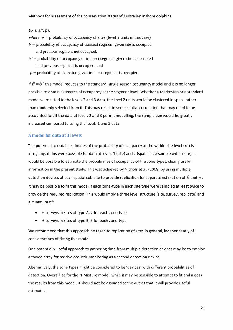
{ , , ', },
probability of occupancy of sites (level 2 units in this case),
probability of occupancy of transect segment given site is occupied
and previous segment not occupied,
' probab
p
where
ility of occupancy of transect segment given site is occupied
and previous segment is occupied, and
probability of detection given transect segment is occupiedp
If ' this model reduces to the standard, single season occupancy model and it is no longer
possible to obtain estimates of occupancy at the segment level. Whether a Markovian or a standard
model were fitted to the levels 2 and 3 data, the level 2 units would be clustered in space rather
than randomly selected from it. This may result in some spatial correlation that may need to be
accounted for. If the data at levels 2 and 3 permit modelling, the sample size would be greatly
increased compared to using the levels 1 and 2 data.
A model for data at 3 levels
The potential to obtain estimates of the probability of occupancy at the within-site level ( ) is
intriguing; if this were possible for data at levels 1 (site) and 2 (spatial sub-sample within site), it
would be possible to estimate the probabilities of occupancy of the zone-types, clearly useful
information in the present study. This was achieved by Nichols et al. (2008) by using multiple
detection devices at each spatial sub-site to provide replication for separate estimation of and p .
It may be possible to fit this model if each zone-type in each site type were sampled at least twice to
provide the required replication. This would imply a three level structure (site, survey, replicate) and
a minimum of:
6 surveys in sites of type A, 2 for each zone-type
6 surveys in sites of type B, 3 for each zone-type
We recommend that this approach be taken to replication of sites in general, independently of
considerations of fitting this model.
One potentially useful approach to gathering data from multiple detection devices may be to employ
a towed array for passive acoustic monitoring as a second detection device.
Alternatively, the zone types might be considered to be ‘devices’ with different probabilities of
detection. Overall, as for the N-Mixture model, while it may be sensible to attempt to fit and assess
the results from this model, it should not be assumed at the outset that it will provide useful
estimates.
Methods for assessment of the conservation status of Australian inshore dolphins
22
It should be recognised that within-site replication of zone types would be very limited and that
confidence intervals would be very wide, although experimenting with the model may provide some
useful insights.
Comment on detection probability and density
While it is not possible to estimate , the probability of occupancy at the secondary sample level, in
the standard, two level, ‘single season’ model, it is useful to note that the estimated probability of
detection p from the model is an estimate of 'p where 'p is the probability of detection given .
The probability of occupancy in a secondary sample is a measure of the rate of use of the
secondary unit and will depend upon the number of groups per unit area (density) present there.
Covariates for sampling units
Current knowledge identifies water depth as an important environmental feature associated with
snubfin habitat selection (Framework; Beasley et al. 2012) but it is not employed as a basic
component of the sampling design in terms of site types, zone types and transect segments. Water
depth and other environmental features may be measured on transect or extracted from available
electronic sources such as bathymetry maps to distinguish among sampling units at each level and
constitute a basis for modelling habitat selection. Covariates may be fitted to both the probability of
occupancy and the probability of detection in occupied sites. Detection covariates would generally
be measured at level 3.
As subsequently described, it is unlikely that data on the level 3 units will be employed directly in
analysis but will more likely be reduced to their means or totals or otherwise scaled for use in a
model for which replicate surveys are at level 2. When replicate surveys are at level 2 rather than
level 3, zone-type and possibly other variables would be employed as detection rather than
occupancy covariates, as described above.
Covariates for primary sampling units (level 1)
Covariates for level 1 units must measure characteristics of the units as wholes. Principally, these
are:
Site type (A, B)
Site area
Areas of each of the zones defined for the site type
Season (date)
Other relevant covariates include:

Methods for assessment of the conservation status of Australian inshore dolphins
23
Areas of water < 10 m and < 20 m deep adjacent to site and between 10 and 20 km from
land (as an indicator of the proportion of a local population that may be more than 10 km
from land at the time of sampling)
Type and extent of human use - recreation, fishing, onshore-offshore pollutant flow
The typical level of boat traffic on a site - this may be associated with detectability through
boat avoidance by populations with little exposure to boats
Bioregion ( http://www.environment.gov.au/resource/guide-integrated-marine-and-coastal-
regionalisation-australia-version-40-june-2006-imcra )
Tidal range, minimum and maximum SST, …
Covariates for secondary sampling units (level 2)
Covariates for level 2 units must measure characteristics of the units as wholes. Principally:
Zone type
Zone area
Length of transect
Characters that vary on a daily scale (see below)
Most fine scale habitat covariates and covariates for detection probability will be measured at level
3. Appropriate covariates for level 2 units may be calculated as totals or means of the values of
covariates measured at level 3:
Occupancy covariates. Mean depth, mean distance from shore, mean distance from nearest
river mouth, mean tidal height, mean tidal state, …
Detection covariates. Total length of transect, mean sea state, mean glare factor, …
Covariates for tertiary sampling units (level 3)
Covariates used to define level 3 units must apply to the units as wholes. This implies measurements
of habitat and detection covariates for each segment (level 3 unit) rather than simply at locations
where groups are detected. These are presence/absence (strictly, detection/non-detection) data and
covariate values are required for each unit of effort whether dolphins were or were not detected.
Two kinds of covariates are appropriate at level 3, those that are potential predictors of occupancy
(presence) and those that are potential predictors of detection when dolphins are present. These
represent within-zone, within-day variation in habitat characters and sighting conditions.
Habitat (occupancy) covariates
1. Distance from nearest river mouth
Methods for assessment of the conservation status of Australian inshore dolphins
24
2. Water depth, tidal state, tide height, distance from land, time of day, …
Detection covariates
3. Sea state (Beaufort), height of observation platform, number of observers, speed of travel,
turbidity, glare factor, …
The latitude and longitude of both the beginnings and ends of transect segments, and sightings
should be recorded. One measure of each covariate per segment should be adequate.
Sample size estimation
Reliable estimates can only be obtained with suitable replication and detection rates. We present
results from a simulation study (Appendix A) based on some available data on snubfin detection
rates using the simple ‘single-season’ occupancy model in the software program Genpres
(http://www.mbr-pwrc.usgs.gov/software/presence.html: Bailey et al. 2007). This model considers
only two levels of replication, sites and surveys (replicates). As indicated above, two-level data may
be derived under either of two scenarios:
1. Scenario 1 - collapsing over the level 3 units (transect segments) within each level 2 unit for
a model using levels 1 (sites) and 2 (replicates or surveys), or
2. Scenario 2 - omitting the level 1 units and using levels 2 (zone-type samples) and 3 (transect
segments) and constructing a spatial dependence model to accommodate the non-
independence in the series of contiguous transect segments (Hines et al. 2010) under an
approach that accommodates the clustering of level 2 units within level 1 units (sites).
We employed the single-season occupancy model (MacKenzie et al. 2002) in our simulations to
generate expectations under both scenarios.
Observed group detection rates and the probability of detection given occupancy
We have summary data from two robust design capture-recapture studies on snubfin dolphins in
which group detections were recorded as part of the sampling protocol:
1. Darwin Harbour and adjacent Bynoe Harbour and Shoal Bay, NT (NT Government Darwin
Harbour Dolphin Monitoring Program: Brooks & Pollock 2013). Estimated abundance = 25,
area = 1000 km2, Group sighting rate = 1 group/195 km transect.
2. Port Essington, Cobourg Peninsula, NT (Palmer et al. 2014). Estimated abundance = 180,
area = 350 km2, Group sighting rate = 1 group/29 km transect.
As the simulation results presented subsequently show, models with detection rates < 0.2 per survey
are very unstable and should be avoided. If the rates of detection per 10 km transect segment in

Methods for assessment of the conservation status of Australian inshore dolphins
25
Darwin and Port Essington (~ 0.05 and ~ 0.30 groups per 10 km respectively) represent extremes
either side of a typical expected value, models based on transect segment data are probably not
viable except in rare circumstances and it should be assumed that level 3 data will need to be
collapsed to level 2 units for analysis (Scenario 1 above) and we proceed on that assumption.
Our interest here is primarily in estimating a minimum number of sites and number of repeat
surveys (level 2) per site to provide estimates of the probability of occupancy with relative standard
errors (or coefficients of variation = ˆ ˆ( ) /SE ) of less than or equal to 0.2. We would like sites like
Darwin which are known to be occupied to have a high probability of being observed to be occupied:
i.e., that there is a low probability that no groups will be observed in any of the set of k repeat
surveys each of a given length of transect. If, as subsequently recommended, each repeat survey is
of a minimum of 40 km of transect, the observed group detection rate d in Darwin would be 40/195
= ~ 0.2 per repeat survey of 40 km.
Each length of transect surveys an area of unknown width depending on how far from the transect
line it is possible for a group to be detected and the probability of detecting a group within that
width. We do not attempt to estimate the effective search width or the effective area surveyed here
but it should be clear that d is associated with the density of groups in the survey area.
Our purpose in this section was to estimate the minimum length of transect required to yield a
detection probability of approximately 0.2 per survey in sites like Darwin which appears to be near
the more thinly populated end of a distribution of site densities. To do this we have made some
unrealistic assumptions such as that groups are uniformly distributed in space so that there is a
probability of sighting one group per 200 km of transect or 0.2 groups per survey of 40 km of
transect wherever a repeat survey is located on the site or whenever it is conducted. Accordingly,
the observed group detection rate d is only an approximate estimate of the parameter of interest,
the probability of detection given occupancy |p .
Partitioning the total number of surveys between sites (level 1) and surveys (level 2)
MacKenzie and Royle (2005) suggest that, for rare species, one should survey more sites less
intensively. While this is sensible for a fixed cost per survey, costs in this study are likely to be
greater in sampling many remote sites less intensively than fewer sites more intensively. MacKenzie
et al. (2006) discuss these issues in their Chapter 6 and indicate that, while following the general
principal of more sites with fewer surveys per site for rare species, allocating relatively more surveys
among fewer sites reduces the false absence rate and is advantageous in identification of habitat
preferences. Some sensible compromise needs to be reached in making this decision; there are
Methods for assessment of the conservation status of Australian inshore dolphins
26
many potential sources of variation that may manifest in the data leaving a lot of room for intuition
and judgement.
For given numbers of sites and surveys per site, increasing the per survey detection rate above 0.2
(preferably to at least 0.4) by completing longer lengths of transect is the only and an effective
means of increasing the precision of the estimated probability of occupancy.
Recommended sample size
In sum, with lengths of transect of at least 40 km in each survey, reasonable relative standard errors
for the estimated probability of occupancy will be achieved when at least 90 sites are surveyed at
least 6 times each for probabilities of occupancy and detection rates per survey of at least 0.2. As
previously, we recommend 6 surveys in sites of type A, 2 for each zone-type, and 6 surveys in sites of
type B, 3 for each zone-type.
For given numbers of sites and surveys per site, increasing the per survey detection rate above 0.2
(preferably to at least 0.4) by completing longer lengths of transect is the only and an effective
means of increasing the precision of the estimated probability of occupancy.
It should be recognised that while 90 sites surveyed 6 times each is a reasonable estimate of the
required sampling intensity for a reasonably precise overall estimate of occupancy across the range,
samples of 30 sites surveyed six times each would probably not constitute a suitable basis for
separate, State-based estimates. With suitable detection rates and probabilities of occupancy
however, 30 sites per State, or 45 sites per site type, each surveyed six times may be adequate to
detect substantial differences in probabilities of occupancy between such categories of sites. This is
part of a general consideration about site covariates for occupancy: there will be limited ability to
model with many covariates simultaneously although a relatively small set of better-fitting
covariates might be selected for fitting in the final model.
We recommend that equal numbers of sites of types A and B be surveyed to maximise the power to
statistically distinguish between them.
Discussion
Considering the potential of aerial survey methods
While Objective 1 clearly specifies a boat-based survey and that is what we have addressed here, the
great size of the extent of occurrence of the species and the remoteness of much of the area
naturally prompt consideration of aerial survey methods. Aerial survey methods were considered at
the Melbourne workshop but much of the discussion was informal and is only briefly commented on

Methods for assessment of the conservation status of Australian inshore dolphins
27
in the workshop report (Department of Environment 2013b) where their ‘apparent unsuitability’ is
referred to (p.5) and they are described as being ‘very expensive and unlikely to be useful for
determining more than the presence/absence of snubfin dolphins’ (p.9).
The potential unreliability of species determination and group size estimation from the air without
extensive and potentially dangerous low-level flying were considered and may have been the
reasons why aerial methods were judged to be apparently unsuitable. This has however not been
carefully assessed for either fixed or rotating wing aircraft.
Determination of presence/absence in a well-defined survey design is the main focus of Objective 1
and it is not clear why not being able to determine more than presence/absence should be
considered a serious limitation of aerial methods provided the reliability of species identification and
group size estimation from the air were established. The relative cost of an aerial and a boat-based
approach to this objective is not obvious and might be the subject of a more formal evaluation.
While it may or may not be the case that an aerial approach would yield reliable data on species and
group sizes, or be more expensive than a boat-based approach to Objective 1, it would seem to
require that a considerable part of the funds to cover the cost of the project be available at once
before the work was undertaken. An aerial approach would also tend to focus the research effort in
the hands of a relatively small group of researchers and probably limit the involvement of
indigenous groups. At the same time, an aerial approach supported with pilot study data and a
financial evaluation may in the end be more efficient than a boat-based approach over such a large
and remote search area. As indicated by the expected group detection rates discussed above, a
boat-based search for such rare animals would involve a lot of searching for relatively few sightings
and be less than satisfying for researchers whose interest is in observing dolphins rather than large
areas of ocean.
Considering the potential of citizen science data
A large amount of data might be collected relatively cheaply in the form of opportunistic sightings by
tourists, fishers, offshore rig workers, indigenous sea ranger groups and others by means of websites
and phone applications. Unlike the sampling design presented here, such data would not be
randomly selected from a sampling frame nor be associated with a direct measure of effort across
the range. While these limitations mean that such data do not meet normal standards for sampling
required to support scientifically rigorous conclusions, potentially many observations could be
collected on an on-going basis.
This sort of opportunistic data may nonetheless be useful; at a minimum it could generate surprises
and fill in gaps in knowledge about the distribution of species of interest. The value of opportunistic

Methods for assessment of the conservation status of Australian inshore dolphins
28
data might be increased if surrogates for effort such as the sizes of and distances to human
populations, fishing fleet sizes and routes, or other data can be developed and incorporated in
models. The utility of such measures might be assessed or improved by calibration against formally
collected presence/absence data with a consistent measure of effort such as the data generated by
the approach described in this report. The results of models based on opportunistic data with
associated proxy measures of effort may become increasingly reliable with on-going calibration
against results from formally-sampled data.
Objective 2: Abundance in selected sites
Background
“Objective 2. To conduct dedicated multi-year studies of the distribution, abundance and habitat use
of snubfin dolphins at selected sites across northern Australia with differing levels of threatening
processes. The studies would provide a plausible estimate of rate of change within sites and by
extension, across the entire range” (Framework p. 3).
Capture-recapture studies
We assume that many marine mammal researchers are familiar with capture-recapture methods,
generally more so than with occupancy methods. Useful general texts for capture recapture models
are Amstrup et al. (2005) and Williams et al. (2002).
Two general types of models (closed and open population models) are used for capture-recapture
data collected over multiple sampling periods to estimate abundance and other demographic
parameters. Closed population models assume that the population remains unchanged for the
duration of the study (i.e. no gains through births or immigration, nor losses through deaths or
emigration). Closed models are applied to short-term studies and can accommodate and explicitly
model variation in capture probabilities by sampling occasion (time), individual animal response
(heterogeneity) and behavioural response to first capture (‘behaviour’ - ‘trap happy’ and ‘trap shy’
responses) (Otis et al. 1978). Un-modelled individual heterogeneity biases abundance estimates
downward, and un-modelled behavioural response to first capture biases abundance estimates
downward if animals became easier to capture (‘trap happy’) or upward if they became harder to
capture (‘trap shy’) following their first capture.
Open-population models allow for demographic changes in the population over time including gains
(births, immigration) and losses (mortality, emigration). Such models can be used to estimate
abundance at each sampling occasion (except the first and last unless a reduced parameter model is

Methods for assessment of the conservation status of Australian inshore dolphins
29
fitted) and the probability of apparent survival (alive and remaining in the sampling area) (Lebreton
et al. 1992) and apparent births (born or immigrated) between sampling occasions (Jolly 1965; Seber
1965; Crosbie & Manly 1985; Arnason & Schwarz 1996).
Open models cannot accommodate variation in capture probabilities except by time, and may
produce biased abundance estimates in the presence of individual heterogeneity or behavioural
response to first capture. As Pollock (1982) argued, apparent survival estimates are robust to these
forms of heterogeneity.
Pollock (1982) proposed a sampling regime (the robust design) of primary samples separated by
time scales that would allow gains and losses from the population, with each primary sample
composed of a set of sufficiently closely spaced secondary samples for population closure to be
assumed. The combination of both open and closed population models within the robust design
allows abundance to be accurately estimated for each primary sampling period in the presence of
heterogeneity and apparent survival to be estimated between primary sampling periods. Kendall et
al. (1995; 1997) and Kendall and Nichols (1997) further developed the robust design model and
incorporated estimation of temporary emigration between primary samples. This is an advance on
standard open-population models in which all immigration and emigration are assumed permanent.
Examples of robust design studies on coastal dolphins include Balmer et al. (2008), Rosel et al.
(2011) and Smith et al. (2013).
Population closure and temporary emigration for coastal dolphin populations
The sizes of the home ranges of local coastal dolphin populations are generally unknown prior to
sampling and the areas of study sites may often be smaller than the areas over which members
range. Movement into and out of the study area during sampling may occur at the two time scales of
a robust design study, between the secondary samples composing the primary sampling periods
(i.e., within primary samples) and between the primary sampling periods as wholes. Such
movements may be random in the sense that there is no temporal structure to the presences and
absences of individuals from the sample area or ‘Markovian’ in the sense that whether an animal is
present in the current period is dependent upon whether it was present in the preceding period.
Markovian movement may be associated with seasons and breeding cycles (Kendall & Bjorkland
2001; Smith et al. 2013).
Movement in and out of the study area within a primary sample constitutes a violation of the
assumption of population closure. An abundance estimate for the primary sample is unbiased
however, provided the movement is random rather than Markovian and the estimate is interpreted
Methods for assessment of the conservation status of Australian inshore dolphins
30
as the number of animals that used the sample area during the primary sampling period (Kendall
1999).
While there are no models for movements within primary samples, movement of portions of the
population in and out of the study area between primary samples may be modelled explicitly as
random or Markovian in the robust design. If such movement is suspected of being associated with
season it may be modelled as such (Smith et al. 2013). Alternatively, if primary samples are taken in
the same season on successive years, seasonal movement would be obviated and the series of
abundance estimates would not be compounded with season-associated temporary emigration. This
would reduce the variation around a trend line fitted to the series of abundance estimates and
increase the precision of the estimated rate of change.
Our assumption is that the large majority of a local population remain within their home range at all
times but may spend periods of time outside the study area. In this case a temporary emigration
estimate describes the proportion of the population that are off the study site (although they may
be nearby) the duration of a primary sample. This will depend on the proportion of the home range
that is within the study area and the relative rates of use of the study area and the remainder of the
home range, which may depend on the relative quality of the habitat in these parts of the home
range or factors influencing the distribution of prey.
General principles for sampling intensity in the robust design
Heterogeneity of capture probabilities due to behavioural response or individual
differences
Apparent behavioural response and apparent individual heterogeneity in capture-recapture studies
based on identification of animals from their natural marks (e.g., photo-id) may arise in the process
of capturing marks, assessing mark quality, and assigning marks to individuals (matching). This
process is subsequently discussed but suffice it to say here that it is preferable to eliminate this
potential source of behavioural and individual heterogeneity at that stage than to model it in the
data. Modelling these forms of heterogeneity comes at the cost of requiring more secondary
samples within each primary sample.
If individual animal characters are associated with their probabilities of capture (e.g., size), it is
preferable that these be measured and modelled as covariates than to employ models to account
for heterogeneity due to unknown sources. While mixture models (Norris & Pollock 1996; Pledger
2000) may be used for this purpose, their performance increases with the number of samples and
may not be viable for fewer than four secondary samples per primary sample.
Methods for assessment of the conservation status of Australian inshore dolphins
31
Number of secondary samples
We recommend that four and preferably more secondary samples be taken per primary sample.
Number of primary samples
While an initial abundance estimate may be made from one primary sample using a closed
population model and a robust design model can be fitted to two, the model becomes increasingly
informative about rates of apparent survival and temporary emigration as the number of primary
samples increases. As subsequently described, estimation of a trend in abundance will generally
require estimates with good precision and a relatively long period of monitoring. We expect reliable
estimates of apparent survival and temporary emigration, and trend to require at least five primary
samples.
Precision of abundance estimates
The two major influences on the precision of abundance estimates are the size of the population
(better precision for larger populations) and the capture rate. While sites where larger populations
are expected might be selected for monitoring, the expected abundances of snubfin populations are
relatively small, leaving increasing the capture probability by more intensive sampling as the only
practical way of increasing the precision of abundance estimates.
The relationship between the precision of a closed population model abundance estimate, relative
standard error (the ratio of the standard error of the estimate to the estimate itself), population size
and capture probability may be seen in Figure 4. These plots were based on sets of 200 simulations
for nine samples estimated with the Simulations facility in program Mark. Relative standard errors of
less than 0.2 represent a target for reasonable precision of abundance estimates but smaller relative
standard errors would increase the probability of detecting changes in abundance. We have
recommended at least four samples per primary period for this study and the estimated relative
standard errors shown in Figure 6 will be optimistic for fewer than nine samples.
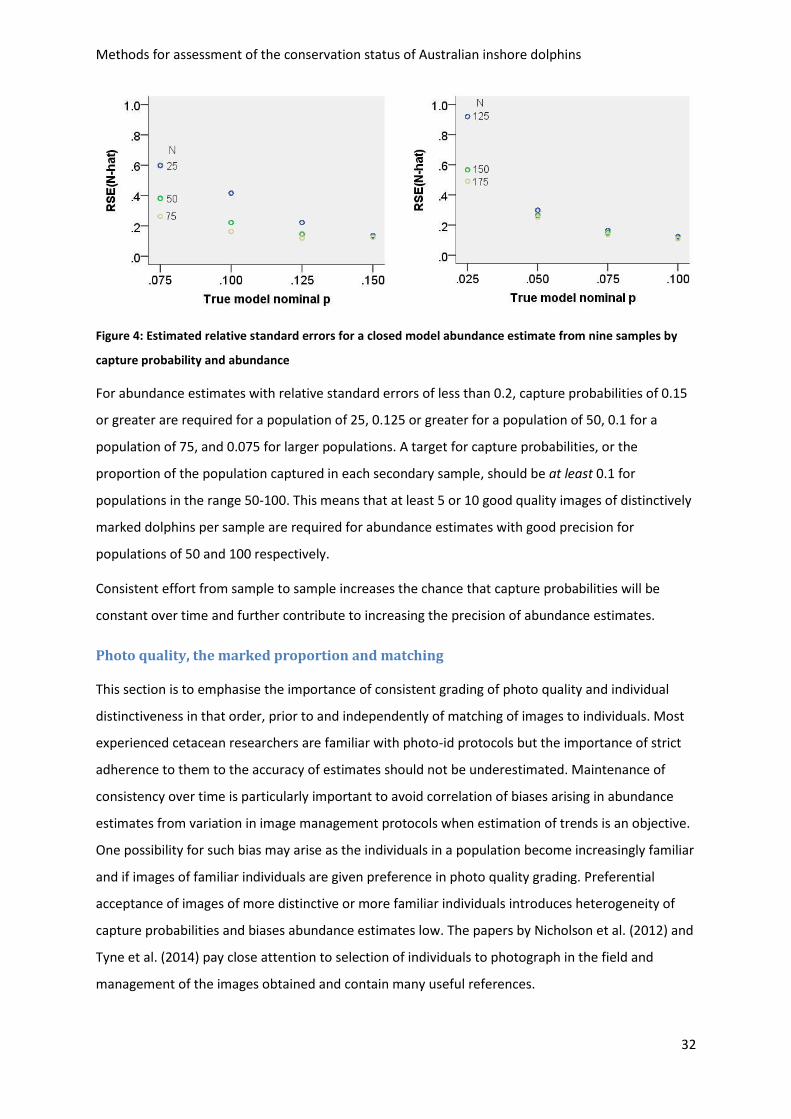
Methods for assessment of the conservation status of Australian inshore dolphins
32
Figure 4: Estimated relative standard errors for a closed model abundance estimate from nine samples by
capture probability and abundance
For abundance estimates with relative standard errors of less than 0.2, capture probabilities of 0.15
or greater are required for a population of 25, 0.125 or greater for a population of 50, 0.1 for a
population of 75, and 0.075 for larger populations. A target for capture probabilities, or the
proportion of the population captured in each secondary sample, should be at least 0.1 for
populations in the range 50-100. This means that at least 5 or 10 good quality images of distinctively
marked dolphins per sample are required for abundance estimates with good precision for
populations of 50 and 100 respectively.
Consistent effort from sample to sample increases the chance that capture probabilities will be
constant over time and further contribute to increasing the precision of abundance estimates.
Photo quality, the marked proportion and matching
This section is to emphasise the importance of consistent grading of photo quality and individual
distinctiveness in that order, prior to and independently of matching of images to individuals. Most
experienced cetacean researchers are familiar with photo-id protocols but the importance of strict
adherence to them to the accuracy of estimates should not be underestimated. Maintenance of
consistency over time is particularly important to avoid correlation of biases arising in abundance
estimates from variation in image management protocols when estimation of trends is an objective.
One possibility for such bias may arise as the individuals in a population become increasingly familiar
and if images of familiar individuals are given preference in photo quality grading. Preferential
acceptance of images of more distinctive or more familiar individuals introduces heterogeneity of
capture probabilities and biases abundance estimates low. The papers by Nicholson et al. (2012) and
Tyne et al. (2014) pay close attention to selection of individuals to photograph in the field and
management of the images obtained and contain many useful references.
Methods for assessment of the conservation status of Australian inshore dolphins
33
Selection of sites for intensive study
Abundance, trends in abundance and threatening processes
It is appropriate that intensive studies be carried out where substantial levels of potentially
anthropogenic impact may be occurring or are likely to occur in the future given that assessment of
the risk to inshore dolphin populations posed by coastal development and human activities is a
primary motivator for the proposed research.
Trends in marine mammal population abundance are extremely difficult to detect unless they are
large (Taylor et al. 2007), especially when populations are small and standard errors are large.
Consequently, it is prudent to select sites for monitoring where trends in abundance and
populations might be expected to be larger to maximise the chance of detecting them. While
estimates of declines in these kinds of sites would not be direct estimates of declines across the
range, selection of such sites for monitoring would target their most likely cause.
Sites might be selected in pairs to compare trends in sites potentially subject to substantial
anthropogenic impact and comparable sites that are not. While the chance of statistically detecting
an overall trend in the set of sites would be greater if the mean trend were greater, suggesting
monitoring only sites where greater declines might be expected, inference to the causes of the
decline would be somewhat stronger in a more experimental design in which trends in ‘impacted’
and ‘non-impacted’ sites were compared. If declines were observed in both anthropogenically-
impacted and non-anthropogenically impacted sites, an argument might be made for an overall
decline not entirely due to direct human impacts.
We recommend that the paired samples approach be adopted while recognising that this may be at
greater risk of not being able to statistically detect an overall trend in order that insight might be
gained into the extent and nature of anthropogenic effects. In doing so however, it should be
recognised that the sample of sites or pairs of sites for intensive monitoring is likely to be small and
statistical power to detect all but strong trends will be limited. If the intensive studies were
implemented on a State-by-State basis, 2 pairs per State would amount to 12 sites overall and 3
pairs per State would amount 18 sites overall.
Paired sites that are reasonably close together are likely to be subject to similar hydrological and
other conditions but may also provide an opportunity to study rates of movement between
populations through close-kin analysis of genetic data or comparison of photo-id catalogues.
Marine parks may be good choices for non-impacted comparison sites as they may be likely to be
accessible and have access to equipment and facilities.
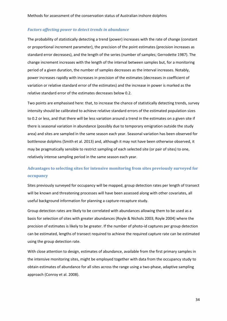
Methods for assessment of the conservation status of Australian inshore dolphins
34
Factors affecting power to detect trends in abundance
The probability of statistically detecting a trend (power) increases with the rate of change (constant
or proportional increment parameter), the precision of the point estimates (precision increases as
standard error decreases), and the length of the series (number of samples; Gerrodette 1987). The
change increment increases with the length of the interval between samples but, for a monitoring
period of a given duration, the number of samples decreases as the interval increases. Notably,
power increases rapidly with increases in precision of the estimates (decreases in coefficient of
variation or relative standard error of the estimates) and the increase in power is marked as the
relative standard error of the estimates decreases below 0.2.
Two points are emphasised here: that, to increase the chance of statistically detecting trends, survey
intensity should be calibrated to achieve relative standard errors of the estimated population sizes
to 0.2 or less, and that there will be less variation around a trend in the estimates on a given site if
there is seasonal variation in abundance (possibly due to temporary emigration outside the study
area) and sites are sampled in the same season each year. Seasonal variation has been observed for
bottlenose dolphins (Smith et al. 2013) and, although it may not have been otherwise observed, it
may be pragmatically sensible to restrict sampling of each selected site (or pair of sites) to one,
relatively intense sampling period in the same season each year.
Advantages to selecting sites for intensive monitoring from sites previously surveyed for
occupancy
Sites previously surveyed for occupancy will be mapped, group detection rates per length of transect
will be known and threatening processes will have been assessed along with other covariates, all
useful background information for planning a capture-recapture study.
Group detection rates are likely to be correlated with abundances allowing them to be used as a
basis for selection of sites with greater abundances (Royle & Nichols 2003; Royle 2004) where the
precision of estimates is likely to be greater. If the number of photo-id captures per group detection
can be estimated, lengths of transect required to achieve the required capture rate can be estimated
using the group detection rate.
With close attention to design, estimates of abundance, available from the first primary samples in
the intensive monitoring sites, might be employed together with data from the occupancy study to
obtain estimates of abundance for all sites across the range using a two-phase, adaptive sampling
approach (Conroy et al. 2008).
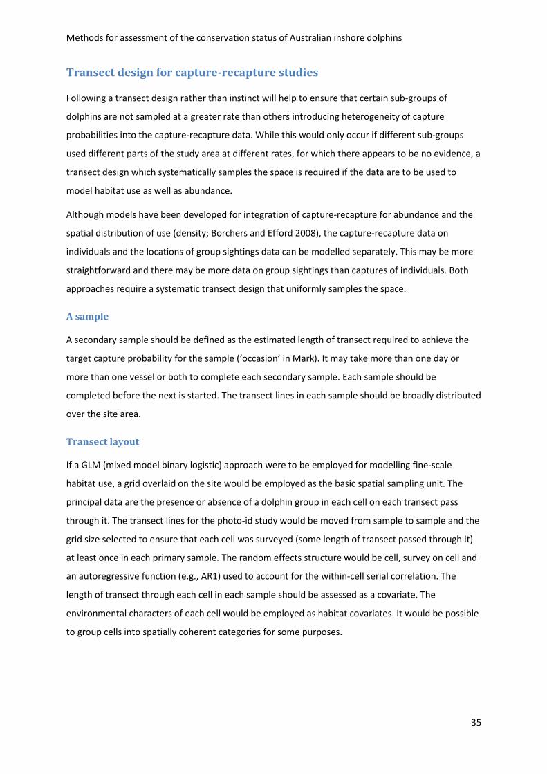
Methods for assessment of the conservation status of Australian inshore dolphins
35
Transect design for capture-recapture studies
Following a transect design rather than instinct will help to ensure that certain sub-groups of
dolphins are not sampled at a greater rate than others introducing heterogeneity of capture
probabilities into the capture-recapture data. While this would only occur if different sub-groups
used different parts of the study area at different rates, for which there appears to be no evidence, a
transect design which systematically samples the space is required if the data are to be used to
model habitat use as well as abundance.
Although models have been developed for integration of capture-recapture for abundance and the
spatial distribution of use (density; Borchers and Efford 2008), the capture-recapture data on
individuals and the locations of group sightings data can be modelled separately. This may be more
straightforward and there may be more data on group sightings than captures of individuals. Both
approaches require a systematic transect design that uniformly samples the space.
A sample
A secondary sample should be defined as the estimated length of transect required to achieve the
target capture probability for the sample (‘occasion’ in Mark). It may take more than one day or
more than one vessel or both to complete each secondary sample. Each sample should be
completed before the next is started. The transect lines in each sample should be broadly distributed
over the site area.
Transect layout
If a GLM (mixed model binary logistic) approach were to be employed for modelling fine-scale
habitat use, a grid overlaid on the site would be employed as the basic spatial sampling unit. The
principal data are the presence or absence of a dolphin group in each cell on each transect pass
through it. The transect lines for the photo-id study would be moved from sample to sample and the
grid size selected to ensure that each cell was surveyed (some length of transect passed through it)
at least once in each primary sample. The random effects structure would be cell, survey on cell and
an autoregressive function (e.g., AR1) used to account for the within-cell serial correlation. The
length of transect through each cell in each sample should be assessed as a covariate. The
environmental characters of each cell would be employed as habitat covariates. It would be possible
to group cells into spatially coherent categories for some purposes.

Methods for assessment of the conservation status of Australian inshore dolphins
36
Objective 3: Spatial and temporal risk assessment of current and
projected threatening processes
We don’t propose to say much about that here except to repeat that a description of the types and
kinds of potential threatening processes should be made prior to sampling so that
Their types and extents might be employed as covariates in the occupancy study under
Objective 1
Sites might be selected for intensive study to represent potentially ‘impacted’ areas under
Objective 2
Methods for assessment of the conservation status of Australian inshore dolphins
37
References
Amstrup, S., T. McDonald, and B. Manly. 2005. Handbook of capture-recapture analysis. Princeton University Press, Princeton, New Jersey, USA.
Arnason, A., and C. Schwarz. 1996. A general methodology for the analysis of capture-recapture experiments in open populations. Biometrics 52:860–873.
Bailey, L. L., J. E. Hines, J. D. Nichols, and D. I. MacKenzie. 2007. Sampling design trade-offs in occupancy studies with imperfect detection: examples and software. Ecological applications : a publication of the Ecological Society of America 17:281–90.
Balmer, B., R. S. Wells, D. Nowacek, L. Schwacke, W. Mclellan, F. Sharf, T. Rowles, L. Hansen, T. Spradlin, and D. Pabst. 2008. Seasonal abundance and distribution patterns of common bottlenose dolphins (Tursiops truncatus) near St. Joseph Bay, Florida, USA. Journal of Cetacean Research and Management 10:157–167.
Beasley, I., S. Allen, and G. J. Parra. 2012. Current status of inshore dolphins in Northern Australia. Final report to Department of Sustainability, Environment, Water, Population and Community.
Brooks, L., and K. H. Pollock. 2013. Abundance, movements and habitat use of coastal dolphins in the Darwin region: Analysis of the first four primary samples (October 2011 to April 2013). Draft report for the Northern Territory Government Department of Landcare Resource Management.
Cagnazzi, D., G. J. Parra, S. Westley, and P. L. Harrison. 2013. At the heart of the industrial boom: Australian snubfin dolphins in the Capricorn Coast, Queensland, need urgent conservation action. PloS one 8:e56729.
Conroy, M. J., J. P. Runge, R. J. Barker, M. R. Schofield, and C. J. Fonnesbeck. 2008. Efficient estimation of abundance for patchily distributed populations via two-phase, adaptive sampling. Ecology 89:3362–70.
Crosbie, S., and B. Manly. 1985. Parsimonious modelling of capture-mark-recapture studies. Biometrics 41:385–398.
Department of the Environment. 2013a. Coordinated research framework to assess the national conservation status of Australian snubfin dolphins (Orcaella heinsohni) and other tropical inshore dolphins.
Department of the Environment. 2013b. Report of the technical workshop on the research strategy to assess the status of the Australian snubfin dolphin (Orcaella heinsohni) and other inshore dolphins.
Gerrodette, T. 1987. A power analysis for detecting trends. Ecology 4:1365–1372.
Guillera-Arroita, G. 2011. Impact of sampling with replacement in occupancy studies with spatial replication. Methods in Ecology and Evolution 2:401–406.
Methods for assessment of the conservation status of Australian inshore dolphins
38
Hines, J. E., J. D. Nichols, J. a Royle, D. I. MacKenzie, a M. Gopalaswamy, N. S. Kumar, and K. U. Karanth. 2010. Tigers on trails: occupancy modeling for cluster sampling. Ecological Applications 20:1456–66.
Jolly, G. 1965. Explicit estimates from capture-recapture data with both death and immigration-stochastic model. Biometrika 52:225–247.
Kendall, K., J. D. Nichols, and J. E. Hines. 1997. Estimating temporary emigration using capture-recapture data with Pollock’s robust design. Ecology 78:563–578.
Kendall, W. L. 1999. Robustness of closed capture-recapture methods to violations of the closure assumption. Ecology 80:2517–2525.
Kendall, W. L., and R. Bjorkland. 2001. Using open robust design models to estimate temporary emigration from capture-recapture data. Biometrics 57:1113–1122.
Kendall, W. L., and J. D. Nichols. 1995. On the use of secondary capture-recapture samples to estimate temporary emigration and breeding proportion. Journal of Applied Statistics 22:751–762.
Kendall, W. L., and G. C. White. 2009. A cautionary note on substituting spatial subunits for repeated temporal sampling in studies of site occupancy. Journal of Applied Ecology:1182–1188.
Lebreton, J.-D., K. P. Burnham, J. Clobert, and D. R. Anderson. 1992. Modeling survival and testing biological hypotheses using marked animals: A unified approach with case studies. Ecological Monographs 62:67–118.
MacKenzie, D. I., L. L. Bailey, and J. D. Nichols. 2004. Investigating species co-occurrence patterns when species are detected imperfectly. Journal of Animal Ecology 73:546–555.
MacKenzie, D. I., J. D. Nichols, G. Lachman, S. Droege, J. A. Royle, and C. Langtimm. 2002. Estimating site occupancy rates when detection probabilities are less than one. Ecology 83:2248–2255.
MacKenzie, D. I., J. D. Nichols, J. A. Royle, K. H. Pollock, L. L. Bailey, and J. E. Hines. 2006. Occupancy estimation and modeling: Inferring patterns and dynamics of species occurrence. Elsevier Publishing Inc.
MacKenzie, D. I., and J. A. Royle. 2005. Designing occupancy studies: general advice and allocating survey effort. Journal of Applied Ecology 42:1105–1114.
Nichols, J. D., L. L. Bailey, F. Allan, O. C. Jr, N. W. Talancy, E. H. C. Grant, A. T. Gilbert, E. M. Annand, and P. Thomas. 2008. Multi-scale occupancy estimation and modelling using multiple detection methods. Journal of Applied Ecology:1321–1329.
Nicholson, K., L. Bejder, S. Allen, M. Krützen, and K. H. Pollock. 2012. Abundance, survival and temporary emigration of bottlenose dolphins (Tursiops sp.) off Useless Loop in the western gulf of Shark Bay, Western Australia. Marine and Freshwater Research 63:1059–1068.
Norris, J., and K. H. Pollock. 1996. Nonparametric MLE under two closed capture-recapture models with heterogeneity. Biometrics 52:639–649.
Methods for assessment of the conservation status of Australian inshore dolphins
39
Otis, D. L., K. P. Burnham, G. C. White, and D. R. Anderson. 1978. Statistical inference from capture data on closed animal populations. Wildlife Monographs 62:1–135.
Palmer, C., L. Brooks, G. J. Parra, T. Rogers, D. Glasgow, and J. Woinarski. 2014. Estimates of abundance and apparent survival of coastal dolphins in Port Essington harbour, Northern Territory, Australia. Wildlife Research In press.
Parra, G. J., C. Azuma, A. R. Preen, P. J. Corkeron, and H. Marsh. 2002. Distribution of Irrawaddy dolphins, Orcaella brevirostris, in Australian waters. Raffles Bulletin of Zoology Supplement 10:141–154.
Parra, G. J., P. J. Corkeron, and H. Marsh. 2006. Population sizes, site fidelity and residence patterns of Australian snubfin and Indo-Pacific humpback dolphins: Implications for conservation. Biological Conservation 129:167–180.
Pledger, S. A. 2000. Unified maximum likelihood estimates for closed capture-recapture models using mixtures. Biometrics 56:434–442.
Pollock, K. H. 1982. A capture-recaptre design robust to unequal probability of capture. Journal of Wildlife Management 46:757–760.
Rosel, P. E., K. D. Mullin, L. P. Garrison, L. Schwacke, J. Adams, B. C. Balmer, P. Conn, M. J. Conroy, T. Eguchi, A. Gorgone, A. Hohn, M. Mazzoil, C. Schwarz, C. Sinclair, T. Speakman, K. Urian, N. Vollmer, P. Wade, R. Wells, and E. Zolman. 2011. Photo-identification capture-mark-recapture techniques for estimating abundance of Bay, Sound and Estuary Populations of Bottlenose dolphins along the U.S. East Coast and Gulf of Mexico: A workshop report NOAA Technical Memorandum NMFS-SEFSC-621. 2011.
Royle, J. A. 2004. N-mixture models for estimating population size from spatially replicated counts. Biometrics 60:108–15.
Royle, J., and J. Nichols. 2003. Estimating abundance from repeated presence-absence data or point counts. Ecology 84:777–790.
Seber, G. 1965. A note on the multiple-recapture census. Biometrika 52:249–259.
Smith, H. C., K. Pollock, K. Waples, S. Bradley, and L. Bejder. 2013. Use of the robust design to estimate seasonal abundance and demographic parameters of a coastal bottlenose dolphin (Tursiops aduncus) population. PloS one 8:e76574.
Taylor, B. L., M. Martinez, T. Gerodette, and J. Barlow. 2007. Lessons from monitoring trends in abundance of marine mammals. Marine Mammal Science 23:157–175.
Tyne, J. a, K. H. Pollock, D. W. Johnston, and L. Bejder. 2014. Abundance and Survival Rates of the Hawai’i Island Associated Spinner Dolphin (Stenella longirostris) Stock. PloS one 9:e86132.
Williams, B. K., J. D. Nichols, and M. Conroy. 2002. Analysis and management of animal populations: modeling, estimation, and decision making. Academic Press.
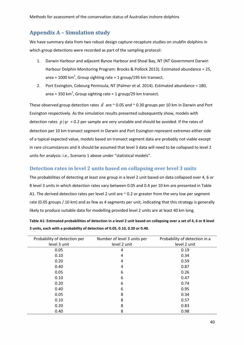
Methods for assessment of the conservation status of Australian inshore dolphins
40
Appendix A – Simulation study
We have summary data from two robust design capture-recapture studies on snubfin dolphins in
which group detections were recorded as part of the sampling protocol:
1. Darwin Harbour and adjacent Bynoe Harbour and Shoal Bay, NT (NT Government Darwin
Harbour Dolphin Monitoring Program: Brooks & Pollock 2013). Estimated abundance = 25,
area = 1000 km2, Group sighting rate = 1 group/195 km transect.
2. Port Essington, Cobourg Peninsula, NT (Palmer et al. 2014). Estimated abundance = 180,
area = 350 km2, Group sighting rate = 1 group/29 km transect.
These observed group detection rates d are ~ 0.05 and ~ 0.30 groups per 10 km in Darwin and Port
Essington respectively. As the simulation results presented subsequently show, models with
detection rates |p < 0.2 per sample are very unstable and should be avoided. If the rates of
detection per 10 km transect segment in Darwin and Port Essington represent extremes either side
of a typical expected value, models based on transect segment data are probably not viable except
in rare circumstances and it should be assumed that level 3 data will need to be collapsed to level 2
units for analysis: i.e., Scenario 1 above under “statistical models”.
Detection rates in level 2 units based on collapsing over level 3 units
The probabilities of detecting at least one group in a level 2 unit based on data collapsed over 4, 6 or
8 level 3 units in which detection rates vary between 0.05 and 0.4 per 10 km are presented in Table
A1. The derived detection rates per level 2 unit are ~ 0.2 or greater from the very low per segment
rate (0.05 groups / 10 km) and as few as 4 segments per unit, indicating that this strategy is generally
likely to produce suitable data for modelling provided level 2 units are at least 40 km long.
Table A1: Estimated probabilities of detection in a level 2 unit based on collapsing over a set of 4, 6 or 8 level
3 units, each with a probability of detection of 0.05, 0.10, 0.20 or 0.40.
Probability of detection per level 3 unit
Number of level 3 units per level 2 unit
Probability of detection in a level 2 unit
0.05 4 0.19 0.10 4 0.34 0.20 4 0.59 0.40 4 0.87 0.05 6 0.26 0.10 6 0.47 0.20 6 0.74 0.40 6 0.95 0.05 8 0.34 0.10 8 0.57 0.20 8 0.83 0.40 8 0.98
Methods for assessment of the conservation status of Australian inshore dolphins
41
Expectations for psi (Ψ)
The point of this exercise is to generate reasonable expectations for the required probability of
occupancy. These estimates can only be made on a highly speculative basis; the areas of sites are
unknown until the sites are defined, local sub-population sizes are likely to be highly variable, the
total number of snubfin is unknown and the proportion of individuals that are mature is not known
accurately.
While we may have different expectations for the probabilities of occupancy in site types A and B it
is useful to consider a typical probability of occupancy for a site and to place this in the context of
the objective of the occupancy study under Criterion 3 (B), in particular that this criterion requires an
estimated total abundance of less than 10,000 mature individuals.
A site extending over 50 km of coast to a distance of 10 km from land would have an area of 500 km2
but sites of type A will be larger as they include at least 100 km2 of within river or inshore, sheltered
area. There are approximately 225,000 km2 in the offshore part of the search area and perhaps
250,000 km2 including inshore sheltered areas. If a typical site were 575 km2, there would be 435
sites in the search area; and if each were occupied by a population of 65 mature individuals, there
would be total of 29,545 mature individuals occupying the search area and a probability of
occupancy of < 0.34 would be required to meet criterion 3 (B).
The sizes of local sub-populations are likely to be highly variable, there may fewer than 10,000
mature individuals and it is prudent to sample for probabilities of occupancy of considerably lower
than 0.35.
It should be clear that these estimates were based on very insecure assumptions (e.g., sub-
population sizes between 50 and 100 individuals, with perhaps 65 mature individuals on average)
and while they may provide an indication of a useful range of occupancy rates for the simulations, a
total abundance of less than or indeed more than 10,000 mature individuals could not be inferred
from the occupancy data alone.
Partitioning the total number of surveys between sites (level 1) and
surveys (level 2)
MacKenzie and Royle (2005) suggest that, for rare species, one should survey more sites less
intensively. While this is sensible for a fixed cost per survey, costs in this study are likely to be
greater in sampling many remote sites less intensively than fewer sites more intensively. MacKenzie
et al. (2006) discuss these issues in their Chapter 6 and indicate that, while following the general
principal of more sites with fewer surveys per site for rare species, allocating relatively more surveys
Methods for assessment of the conservation status of Australian inshore dolphins
42
among fewer sites reduces the false absence rate and is advantageous in identification of habitat
preferences. Some sensible compromise needs to be reached in making this decision; there are
many potential sources of variation that may manifest in the data leaving a lot of room for intuition
and judgement.
The simulation set
We assumed a broad range of values for each of the number of sites, the number of surveys per site
(replicates), the probability of occupancy, and detection rates, specifically:
Sites {15, 30, 45, 60, 90}
Surveys per site ( k ) {4, 6, 8}
Occupancy (ψ) {0.2, 0.3, 0.5}
Detection probability ( |p p ) {0.1, 0.2, 0.4, 0.6, 0.8}
One thousand (1000) simulations were run for each of the 225 combinations (simulation sets) of
these assumed true values. The results were summarised for each simulation set terms of:
The number of models for which psi was estimated as either 0 or 1. We considered these to
be failures (‘fail.psi’) and set an arbitrary maximum of 5% as a target for descriptive
purposes.
The mean estimated probability of occupancy ˆ( ( ))mean
The mean standard error of the estimated probability of occupancy ˆ( ( . ))mean se
The relative standard error (mean coefficient of variation) of the probability of occupancy
ˆ ˆ ˆ( . ( . ))rse mean se . We set an arbitrary maximum of 25% as a target for descriptive
purposes. Note that an alternative formula ˆ ˆ ˆ( . . ( ))rse sd mean produced very similar
results.
The relative standard error from each simulation set is plotted by the number of sites surveyed, the
number of surveys (replicates k ) per site, the probability of detection per survey ( |p ) and the
probability of occupancy ( ) in Figure A1. At a per survey probability of detection rate of 0.2, the
relative standard errors are reasonable (< 0.25) for as few as 90 sites each surveyed as few as six
times for probabilities of occupancy as low as 0.3. At a per survey detection rate of 0.4, the relative
standard errors are reasonable (< 0.25) for as few as 90 sites each surveyed at as few as six times for
probabilities of occupancy as low as 0.2
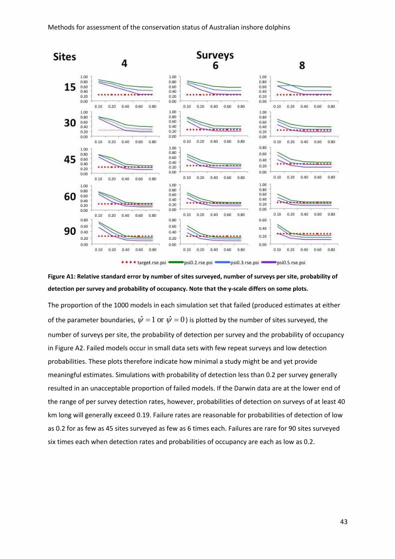
Methods for assessment of the conservation status of Australian inshore dolphins
43
Figure A1: Relative standard error by number of sites surveyed, number of surveys per site, probability of
detection per survey and probability of occupancy. Note that the y-scale differs on some plots.
The proportion of the 1000 models in each simulation set that failed (produced estimates at either
of the parameter boundaries, ˆ ˆ1 or 0 ) is plotted by the number of sites surveyed, the
number of surveys per site, the probability of detection per survey and the probability of occupancy
in Figure A2. Failed models occur in small data sets with few repeat surveys and low detection
probabilities. These plots therefore indicate how minimal a study might be and yet provide
meaningful estimates. Simulations with probability of detection less than 0.2 per survey generally
resulted in an unacceptable proportion of failed models. If the Darwin data are at the lower end of
the range of per survey detection rates, however, probabilities of detection on surveys of at least 40
km long will generally exceed 0.19. Failure rates are reasonable for probabilities of detection of low
as 0.2 for as few as 45 sites surveyed as few as 6 times each. Failures are rare for 90 sites surveyed
six times each when detection rates and probabilities of occupancy are each as low as 0.2.
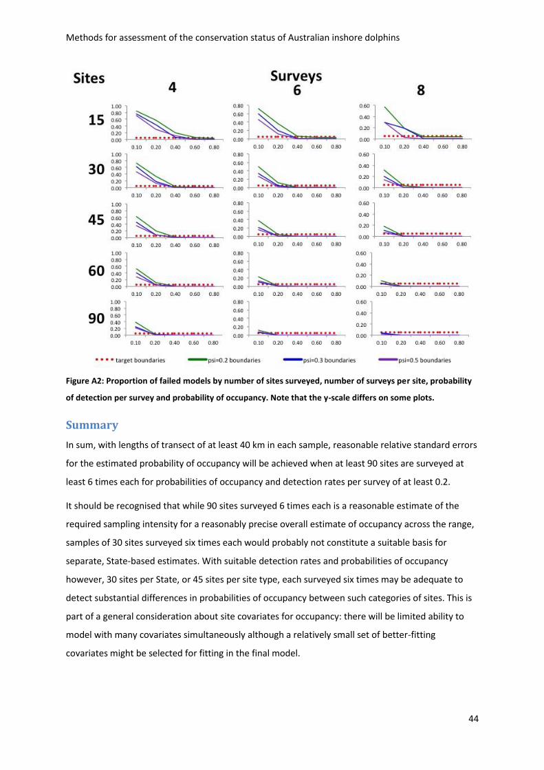
Methods for assessment of the conservation status of Australian inshore dolphins
44
Figure A2: Proportion of failed models by number of sites surveyed, number of surveys per site, probability
of detection per survey and probability of occupancy. Note that the y-scale differs on some plots.
Summary
In sum, with lengths of transect of at least 40 km in each sample, reasonable relative standard errors
for the estimated probability of occupancy will be achieved when at least 90 sites are surveyed at
least 6 times each for probabilities of occupancy and detection rates per survey of at least 0.2.
It should be recognised that while 90 sites surveyed 6 times each is a reasonable estimate of the
required sampling intensity for a reasonably precise overall estimate of occupancy across the range,
samples of 30 sites surveyed six times each would probably not constitute a suitable basis for
separate, State-based estimates. With suitable detection rates and probabilities of occupancy
however, 30 sites per State, or 45 sites per site type, each surveyed six times may be adequate to
detect substantial differences in probabilities of occupancy between such categories of sites. This is
part of a general consideration about site covariates for occupancy: there will be limited ability to
model with many covariates simultaneously although a relatively small set of better-fitting
covariates might be selected for fitting in the final model.