Embed Size (px)
Citation preview

Scholars' Mine Scholars' Mine
Masters Theses Student Theses and Dissertations
Summer 2013
Methods for evaluating effect of operators on drag line energy Methods for evaluating effect of operators on drag line energy
efficiency efficiency
Maryam Abdi Oskouei
Follow this and additional works at: https://scholarsmine.mst.edu/masters_theses
Part of the Mining Engineering Commons
Department: Department:
Recommended Citation Recommended Citation Abdi Oskouei, Maryam, "Methods for evaluating effect of operators on drag line energy efficiency" (2013). Masters Theses. 7141. https://scholarsmine.mst.edu/masters_theses/7141
This thesis is brought to you by Scholars' Mine, a service of the Missouri S&T Library and Learning Resources. This work is protected by U. S. Copyright Law. Unauthorized use including reproduction for redistribution requires the permission of the copyright holder. For more information, please contact [email protected].

METHODS FOR EVALUATING EFFECT OF OPERATORS ON DRAGLINE
ENERGY EFFICIENCY
by
MARY AM ABDI OSKOUEI
A THESIS
Presented to the Faculty of the Graduate School ofthe
MISSOURI UNIVERSITY OF SCIENCE AND TECHNOLOGY
In Partial Fulfillment of the Requirements for the Degree
MASTER OF SCIENCE IN MINING ENGINEERING
2013
Approved by
Kwame Awuah-Offei, Advisor Samuel Frimpong Mariesa L. Crow

lll
ABSTRACT
Draglines are dominant machines and the most significant electricity consumers
in surface coal mines. With the growing price of energy, environmental concerns, and the
high sensitivity of mine profitability to dragline productivity, any improvement in
efficiency of dragline will be beneficial for mines. Research has shown that operator
practices have a significant impact on energy efficiency of mining loading tools.
However, not enough work has been done to provide guidance on how to quantitatively
assess the effect of operator practices on dragline energy efficiency.
The objectives ofthis work were to: (i) test the hypothesis that dragline operator's
practices and skills significantly affect dragline energy efficiency; and ( ii) develop a
methodology to identify the critical parameters that explain the differences in operator
energy efficiency. Statistical tests are suggested to study the effect of operator practice
and skills on dragline energy efficiency to achieve the first research objective. The
second objective was achieved with a novel methodology based on sound statistical
principles. Both approaches were illustrated with a real-life dragline operation. The
suggested methodology was used on the data collected from an 85yd3 BE-1570w dragline
to compare the energy efficiency of five operators during a one month period.
Valid methods have been formulated for testing operator effects on dragline
energy efficiency and for identifying critical parameters that explain such differences.
Using the developed approaches, the case study shows that operator practices can affect
dragline energy efficiency. The tests show that there is a high probability that differences
in energy efficiency are due to dumping height, vertical and horizontal drag distances,
and spotting and dumping time among the surveyed operators.

lV
ACKNOWLEDGEMENTS
I would like to express my deepest gratitude to all who helped and supported me
to finish my thesis. First and foremost, I would like to appreciate my graduate advisor Dr.
Kwame Awuah-Offei for his constant support and guidance on pursuing my thesis.
Furthermore, I would like to acknowledge my graduate committee members: Dr.
Samuel Frimpong and Dr. Mariesa Crow for their support and interest in my research. I
would like to extend my sincere appreciation to Dr. Akim Adekpedjou for his corporation
and invaluable inputs.
Also, I would like to appreciate Department of Mining Engineering in Missouri
University of Science and Technology for giving me the opportunity to pursue my
graduate studies. Ms. Barbara Robertson, Ms. Shirley Hall, Ms. Leanne Nuckolls, Ms.
Diane Henke, and Mrs. Judy Russell for the technical support and other administrative
assistances
Last but not least, I would like to appreciate my mother for her unconditional
love, my father for his support, my sister and Ms. Negin Sobhani for their endless
encouragements at different stages of my life.

v
TABLE OF CONTENTS
Page
ABSTRACT .............................................................................................................. iii
ACKNOWLEDGEMENTS ....................................................................................... iv
LIST OF ILLUSTRATIONS ................................................................................... viii
LIST OF TABLES ...................................................................................................... x
NOMENCLATURE ................................................................................................. xii
SECTION
1. INTRODUCTION ................................................................................................ . 1
1.1. BACKGROUND ........................................................................................... I
1.2. STATEMENT OF PROBLEM ...................................................................... 3
1.3. OBJECTIVES AND SCOPE OF THIS RESEARCH .................................... 6
1.4. RESEARCH METHODOLOGY ................................................................... 7
1.5. STRUCTURE OF THE THESIS ................................................................... 9
2. LITERATURE REVIEW ...................................................................................... 10
2.1. DRAGLINE OPERATION ............................................................................ 10
2.2. SIGNIFICANCE OF ENERGY EFFICIENCY .............................................. 13
2.3. DRAG LINE ENERGY EFFICIENCY ........................................................... 17
2.4. DRAG LINE ENERGY MONITORING ......................................................... 20
2.5. FACTORS AFFECTING DRAGLINE ENERGY EFFICIENCY ................... 23
2.5.1. Important KPis ........................................................................................ 23
2.5.1.1 Payload .......................................................................................... 23
2.5.1.2 Cycle time ..................................................................................... 24

VI
2.5.1.3 Digging time and digging energy ................................................... 25
2.5.1.4 Fill factor ....................................................................................... 25
2.5.1.5 Engagement/disengagement position .............................................. 26
2.5.2. Governing Parameters ............................................................................. 26
2.5.2.1 Operating conditions ...................................................................... 26
2.5.2.2 Mine design and planning .............................................................. 27
2.5.2.3 Equipment characteristics .............................................................. 27
2.5.2.4 Operators practice .......................................................................... 27
2.6. ASSESSING THE EFFECT OF OPERA TOR'S PRACTICE ......................... 29
2.7. SUMMARY ................................................................................................... 32
3. FIELD DATA ACQUISITION FOR CASE STUDIES .......................................... 34
3.1. STUDY SITE ................................................................................................. 34
3.1.1. Geology .................................................................................................. 34
3.1.2. Mine Operations ..................................................................................... 36
3.2. FIELD EXPERIMENT .................................................................................. 37
3.3. SUMMARY ................................................................................................... 42
4. PRELIMINARY DATA ANALYSIS OF FIELD DATA ...................................... .43
4.1. STRUCTURE OF DATASET ........................................................................ 43
4.2. DETECTING AND REMOVING OUTLIERS ............................................. .46
4.3. DRAGLINE OPERATORS ........................................................................... 48
4.4. SUMMARY .................. ." ................................................................................ 52
5. EFFECTS OF OPEARTOR PRACTICE ON DRAGLINE ENERGY EFFICIENCY ....................................................................................................... 54
5.1. DRAGLINE ENERGY EFFICIENCY ........................................................... 54

Vll
5.2. EVALUATING THE EFFECT OF OPERATOR PRACTICE ON DRAG LINE ENERGY EFFICIENCY ............................................................................... 56
5.2.1. Preliminary Data Analysis ....................................................................... 57
5.2.2. Test for Equality ofMeans ...................................................................... 59
5.3. CASE STUDY ............................................................................................... 64
5.3.1. Preliminary Data Analysis ....................................................................... 64
5.3.1. Test for Equality ofMeans ...................................................................... 69
5.4. SUMMARY ................................................................................................... 71
6. IDENTIFYING PARAMETERS THAT CAUSE DIFFERENCES BETWEEN ENERGY EFFICIENCY OF OPERATORS ......................................................... 73
6.1. INTRODUCTION ......................................................................................... 73
6.2. CORRELATION ANALYSIS ....................................................................... 73
6.3. IDENTIFYING RESPONSIBLE PARAMETERS ......................................... 75
6.4. CASE STUDY ............................................................................................... 80
6.5. SUMMARY ................................................................................................... 89
7. CONCLUSIONS AND RECOMMENDATIONS ................................................. 91
7.1. SUMMARY ................................................................................................... 91
7.2. CONCLUSIONS ............................................................................................ 92
7.3. RECOMMENDATIONS FOR FUTURE WORK .......................................... 96
APPENDICES
A. LIST OF 44 PARAMETERS IN THE DATABASE ....................................... 98
B. EXPERIMANT AL FIELD DATA ................................................................ 1 00
BIBLIOGRAPHY ................................................................................................... 1 02
VITA ...................................................................................................................... 110

viii
LIST OF ILLUSTRATIONS
Page
Figure 1-1 Factors affecting energy efficiency (adapted from (K. Awuah-Offei et al., 2011)) ....................................................................................................................... 6
Figure 1-2 Activities/task in this research ........................................................................ 8
Figure 2-1 Schematic view of dragline ........................................................................... lO
Figure 2-2 Dragline cycle .............................................................................................. 11
Figure 2-3 Simple side casting method .......................................................................... 12
Figure 2-4 Energy Consumption 2011(Quadrillion Btu) (U.S. Energy Information Administration (EIA), 2011c) .................................................................................. 13
Figure 2-5 World energy demand, adapted from (Exxon Mobil, 2013) ........................... 15
Figure 2-6 Energy requirement for coal mining (TBtulton of coal) (U.S. Department of Energy(DOE), 2007) ............................................................................................... 17
Figure 2-7 Factors affecting dragline productivity and energy consumption ................... 24
Figure 3-1 Coal stratigraphy in the Gillette coalfield (adapted from (USGS, 2008)) ....... 36
Figure 3-2 Mining sequence in the mine ........................................................................ 39
Figure 3-3 Schematic representation of dragline drive .................................................. .40
Figure 4-1 Drag line cycle components .......................................................................... .44
Figure 4-2 Boxplot defmition in this work ..................................................................... 47
Figure 4-3 Boxplots ofrelevant parameters before removing any outlier ....................... .49
Figure 4-4 Boxplots ofrelevant parameters after removing outliers ............................... 50
Figure 4-5 Mean standard error and number of cycles of all operators ........................... 51
Figure 4-6 Mean standard error and number of cycles of eight operators ........................ 52
Figure 5-1 Process for evaluating operator effects on dragline energy efficiency ............ 57

lX
Figure 5-2 Algorithm of choosing an appropriate test of comparing the means (more than two groups) ............................................................................................................. 61
Figure 5-3 Algorithm of choosing an appropriate test of comparing the means (two groups) .................................................................................................................... 63
Figure 5-4 Histograms of energy efficiency of different operators .................................. 65
Figure 5-5 Histograms oflog-transformed energy efficiency of different operators ........ 66
Figure 5-6 Q-Q plot of energy efficiency ....................................................................... 69
Figure 5-7 Q-Q plot oflog-transformed data .................................................................. 70
Figure 6-1 Flow chart of the main algorithm .................................................................. 74
Figure 6-2 Algorithm of using linear regression of differences to find significant parameters ............................................................................................................... 81
Figure 6-3 Estimated probability for correlated parameters to be responsible parameter.85

X
LIST OF TABLES
Page
Table 1-1 Coal reserves, production and consumption by countries (2011) (British Petroleum (BP), 2012),(U.S. Energy Information Administration (EIA), 2011a) ....... 1
Table 1-2 U.S. coal consumption by end use sector (2011 and 2010) (U.S. Energy Information Administration (EIA), 2011b) ................................................................ 2
Table 1-3 Annual energy consumption by commodity type (U.S. Department of Energy(DOE), 2007) ................................................................................................. 4
Table 3-1 Operating specifications of a Bucyrus-Erie 1570W dragline .......................... 38
Table 3-2 Electrical configuration of dragline motors/generators ................................... 38
Table 4-1 Relevant Parameters ..................................................................................... .45
Table 4-2 Classification ofthe data based on number ofbucket reloads ....................... .46
Table 4-3 Operator activity ........................................................................................... .48
Table 4-4 Standard error ................................................................................................ 53
Table 5-1 Summary of operators performance ............................................................... 55
Table 5-2 Descriptive statistics of energy efficiency of operators ................................... 64
Table 5-3 Results ofthe statistical tests on original data and log-transfomed data .......... 67
Table 5-4 Result of the statistical test ............................................................................. 70
Table 6-1 Pattern of the data set ..................................................................................... 76
Table 6-2 Difference matrix of operator i and j .............................................................. 78
Table 6-3 Output of coefficient test for one pair.. ........................................................... 78
Table 6-4 Output of coefficient test and final conclusion of k runs (one pair) ................. 79
Table 6-5 Pearson correlation result ............................................................................... 82

Table 6-6 Results ofthe 30 times run of regression analysis. Numbers indicate the number of times that a parameter is recognized as a parameter with significant
xi
coefficient (responsible parameter) .......................................................................... 84
Table 6-7 Final result based on assigning 0 and 1 .......................................................... 87

Xll
NOMENCLATURE
Page
Eout_drag: Output energy of drag motors ...................................................................... 18
W drag_ bucket: Work done to drag the bucket ................................................................. 18
Wctrag_materiat: Work done to drag materal .................................................................... 18
Wresistance: Work done to overcome the resistance of the material ............................... 18
Wtriction: Work done to overcome the friction between material and the bucket ........... 18
Eout_hoist: Output energy of hoist motors ..................................................................... 18
Whoist_materiat: Work done to overcome the weight ofthe bucket .................................. 18
Whoist_bucket: Work done to overcome the weight ofthe bucket ................................... 18
Whoist_chains: Work done to overcome the weight ofthe chains .................................... 18
Eout_swing: Output energy of swing motors .................................................................. 19
'tswing :Swing motor torque ......................................................................................... 19
8swing: Angular displacement ofthe machine ............................................................. 19
11: Energy efficiecy .................................................................................................... 20
P: Payload ................................................................................................................. 20
E1: Total energy consumption .................................................................................... 20
nop: Number ofoperators .......................................................................................... 30
OPI: Operator performance indicator. ........................................................................ 31
Ss: Sample standard deviation ................................................................................... 31
OPis: mean sample mean .......................................................................................... 31
Q 1: First quartile ........................................................................................................ 46
Q3: Third quartile ...................................................................................................... 46

X Ill
SEi: Standard Error .................................................................................................... 52
nOc: Number ofcycles .............................................................................................. 52
Es: Swing energy ....................................................................................................... 55
Ect: Drag energy ......................................................................................................... 55
Eh: Hoist energy ........................................................................................................ 55
nOp: Number ofoprators ........................................................................................... 59
a: Significanct level. .................................................................................................. 60
cr: Standard deviation ................................................................................................. 75
p: Pearson correlation coefficient .............................................................................. 75
S1: Spot time ............................................................................................................. 83
00 : Swing out angle ................................................................................................... 83

1. INTRODUCTION
1.1. BACKGROUND
Coal has been known as an important energy source for years. Today, coal is
mostly used as a fuel for electric power generation, although, its significant historical role
in industrial, transportation, and domestic heating cannot be denied. The United States
(U. S.), Russia and China have the largest known coal reserves. 237 billion tonnes of
proven recoverable coal reserves (27.6% ofthe global total) is located in U.S. The total
coal consumption in the U.S. during 2011 was 909.9 million tonnes (U.S. Energy
Information Administration (EIA), 2011a) and the total production was 992.8. In 2010,
U.S. share oftotal global coal production was 13.5% (British Petroleum (BP), 2012).
Table 1-1 shows the coal reserves, production and consumption oftop five countries in
the world.
Table 1-1 Coal reserves, production and consumption by countries (2011) (British Petroleum (BP), 2012),(U.S. Energy Information Administration (EIA), 2011a)
Proven Reserves Coal Production Coal Consumption
Country (Million tonnes) (Million tonnes) (Million tonnes)
u.s. 237,295 992.8 909.9
Russia 57,010 333.5 237.7
China 114,500 3520 3,676.8
Australia 76,400 415.5 129.3
India 60,600 588.5 714.9
Total World 860,938 7,695.4 7,252.9

2
Coal end uses in the U.S. can be classified into three groups; steam coal,
metallurgical coal (coke), and industrial coal. Steam coal is used to produce heat or steam
for industrial processes in power plants and counts for about 90% of total coal
consumption. This share varies depending on natural gas price, which is a substitute fuel
for coal in power plants. Metallurgical coal or coke is used in blast furnaces in standard
iron smelting to produce steel. Industrial coal provides the heat for industrial processes in
manufacturing plants, papers mills, food processors, and cement and limestone plants
(World Energy Council, 2010). The recorded coal consumption in each group is
displayed in Table 1-2.
Table 1-2 U.S. coal consumption by end use sector (2011 and 2010) (U.S. Energy Information Administration (EIA), 2011b)
Metallurgical Industrial
End use sector Electric Power Coal (coke) Coal
Coal consumption (thousand 932,484 21,434 49,031
short tons)- 2011
Coal consumption (thousand 975,052 21,092 52,370
short tons)- 20 10
The coal mining method is chosen based on the depth, thickness and dip of coal
seams, economic studies, and environmental concerns. Coal mining methods generally
fall into two groups: surface and underground mining. In 1973, surface and underground
coal mines both had equal share in total U.S. coal production. Large scale mining
technology enabled coal mines to increase their production, especially in surface coal

3
mines. In 2011, 68% oftota1 coal was extracted using surface coal mines (U.S. Energy
Information Administration {EIA), 2011b). Increasing mine productivity helps the mining
industry to satisfy the growing demand for coal. Larger surface coal mines, utilizing
larger and more efficient equipment with advanced control systems are known factors
that improve mine productivity (Bonskowski, Watson, & Freme, 2006). The efficiency
and environmental impacts of surface coal mining is, therefore, very important for the
continued significance of coal.
1.2. STATEMENT OF PROBLEM
In 2007, the energy consumed in the U.S. mining industry is estimated to be 365
billion kWh (U.S. Department ofEnergy(DOE), 2007). Table 1-3 shows the estimated
annual energy consumption by commodity group. Energy consumption in coal mines is
estimated as 142 billion kWh per year. Electric equipment used for materials handling in
coal mines consumes 13.3 billion kWh, annually (U.S. Department ofEnergy(DOE),
2007). Considering the average price of electricity for industry ( 6.65 cents/kwh in 2011
(U.S. Energy Infromation Administration, 2012)), the cost of electricity for materials
handling in coal mines is $884 million each year. This accounts for 28% oftotal annual
energy cost in the U.S. mining industry.
Draglines are dominant machines and the most critical units in mines, with capital
cost of$50-100 million (Demirel & Frimpong, 2009; Kizil, 2010). The advantages of
dragline mining systems include low mining cost, high production rate, and compatibility
with wide range of overburden depth and material characteristics (Humphrey, 1990).
Draglines are the most significant electricity consumers in surface coal mines. With the

4
high capital investment, growing price of energy, and the high sensitivity ofmine
profitability to dragline productivity any improvement in efficiency and productivity of
draglines will be beneficial for mines. In the Australian coal mining industry, one percent
increase in dragline productivity is valued at $50,000 to $2,300,000, annually (G.
Lumley, 2005).
Table 1-3 Annual energy consumption by commodity type (U.S. Department of Energy(DOE), 2007)
Energy consumption Energy consumption
Commodity Type (Trillion Btulyr) (Million kWh/yr)
Coal 485.3 142.2
Metals 553.1 162.1
Minerals 208.9 61.2
Total 1246.3 365.2
U.S. Department ofEnergy (DOE) carried out studies to show the total energy
saving opportunities in energy-intensive industries, which can be achieved by improving
current processes by implementing energy efficient practices. Their studies show that 70
billion kWh (49% oftotal energy consumption in coal mining) or $3.7 billion can be
saved annually in the U.S. coal mining industry by improving energy efficiency and
implementing best practices (Bonskowski et al., 2006; Humphrey, 1990). Due to the
increasing cost of energy and growing concerns about energy availability and supply,
managing energy efficiency has become a serious issue in surface coal mines (K. Awuah-

5
Offei, Osei, & Askari-Nasab, 2011). Bogenovic (2008) indicated that reduction in energy
consumption and energy cost can be achieved by effective energy management systems
in the way of measuring that measure energy consumption to identify energy saving
opportunities and high-energy consumption units, and determining the relation between
production and energy consumption (Bogunovic, 2008).
Generally, energy efficiency is described as the ratio ofuseful work done (energy
output) to the input energy (Zhu & Yin, 2008). In cases where either energy output or
input cannot be measured easily, proxy parameters are used in their place. Dragline
energy efficiency is defined as the ratio oftotal weight of removed material (payload) to
total energy consumed to remove this amount of material. Dragline energy efficiency
depends on the equipment, operating conditions, and the operator (Figure 1-1).
For a given mine with a selected dragline, optimizing the dragline drive
mechanism for energy efficiency can be very expensive. Mine planning can be used to
reduce the effect of operating conditions on energy efficiency. However, due to the effect
of geology, which cannot be changed for a mine, operating conditions can only yield so
much energy efficiency. Research has shown that operator practices have a significant
impact on energy efficiency of mining loading tools (Bogunovic, Kecojevic, Lund,
Heger, & Mongeon, 2009; G. Lumley, 2005; Patnayak, Tannant, Parsons, Del Valle, &
Wong, 2007). For instance, Bogunovic (2008) and Komljenovic et al. (2010) showed
that dragline productivity can be significantly different for different operators under the
same operation conditions (Bogunovic, 2008; Komljenovic, Bogunovic, & Kecojevic,
201 0). Hence, a better understanding of the relationship between operator practices and
energy efficiency can easily yield significant improvements in energy efficiency and

costs. However, not enough work has been done to quantitatively assess the effect of
operator practices on dragline energy efficiency and the reasons for such variations.
Previous work has demonstrated the significant effect of operator's skills and practice on
dragline productivity. In this study the relation between operators' practice and dragline
energy efficiency is investigated using statistical tools. The goal is to develop a
methodology to evaluate the effect of operator practice on dragline energy efficiency.
Operator
Experiment
Preferences
Interaction with other equipment
Operating condition
Mine conditions
Age
Energy consumption
Technology
411 Energy source
Equipment
Figure 1-1 Factors affecting energy efficiency (adapted from (K. Awuah-Offei et al., 2011))
1.3. OBJECTIVES AND SCOPE OF THIS RESEARCH
The primary objective of this study was to describe the impact of operator
practices on dragline energy efficiency. The specific objectives of this project were to:
6

7
1. Test the hypothesis that dragline operator's practices and skills significantly affect
dragline energy efficiency; and
2. Develop a methodology to identify the critical parameters that explain the
differences in operator energy efficiency.
All the tests and studies in this work were carried out on a dataset obtained from a
specific dragline. The monitoring system ofthe dragline was limited in the number of
recording parameters. For this reason the results of the second objective is limited to the
recorded parameters in dragline's database.
1.4. RESEARCH METHODOLOGY
Figure 1-2 presents the research framework adopted in this work. Statistical tests
are suggested as a tool to study the effect of operator practice and skills on drag line
energy efficiency to achieve the first research objective. The second objective was
achieved with a novel methodology based on sound statistical principles. Both
approaches were illustrated with a real-life dragline operation. The data used as a case
study was collected from a Bucyrus-Erie 1570w (85 yd3 bucket) dragline operating in a
coal mine in Wyoming during one month. The suggested methodology was used on this
data to compare the energy efficiency of five operators during the one month period of
data collection. SAS® (SAS Institute inc., 2011) and MATLAB (The Math Works Inc.,
2011) were used to apply the methodology on the given data.
The methods proposed to evaluate operator effects on dragline energy efficiency
(objective one) make use of parametric and non-parametric statistical test for comparing
means of groups of data. The challenges for using such tests on field obtained dragline

energy efficiency data include data preparation, normality of data, and equality of
variances. The approach suggested in this work systematically checks all these
assumptions and minimizes their effect on the inferences drawn.
Study the effects of operator practice on
energy efficiency
Method to identify critical parameters
explaining the differences in
operator energy efficiency
Field study
Figure 1-2 Activities/task in this research
8

9
The methods proposed to identify key parameters that lead to differences in
operator performance make use of regression analysis of difference data to predict causes
of under- or over-performance. The main challenge in using this approach for field
obtained dragline energy efficiency data is the prevalence of missing data (Schafer &
Graham, 2002) when preparing the difference data. Theoretically sound techniques are
used to hypothesize the pattern or distribution of missingness, which is validated with the
case study data. Random sampling techniques are used to generate equal number of
samples for each pair of operators to generate the difference data for investigation. The
proposed methods are illustrated with the case study data.
1.5. STRUCTURE OF THE THESIS
This thesis contains seven sections. Section 2, literature review, covers a review
of relevant previous work. Information about the mine, the dragline and the dragline
monitoring system used for the case studies in this work is provided in Section 3. In
Section 4 the preliminary statistical analysis ofthe data used in the case studies, such as
analyzing the structure of the dataset, and detecting and removing outliers, is presented.
Section 5 discusses the effects of operator's skills on dragline energy efficiency
(objective one). The section presents a methodology and a case study to illustrate it.
Section 6 presents a methodology (and a case study) for examining which of the recorded
parameters is responsible for observed differences in operator energy efficiencies
(objective two). Section 7 provides the conclusions ofthis study and recommendations
for future work.

10
2. LITERATURE REVIEW
2.1. DRAGLINE OPERATION
Draglines are the most dominant and critical machines in strip mines, commonly
used for clearing the overburden to expose coal seams for extraction. Some properties of
dragline operation include simple and low cost operation, high production rate, simple
mine planning, and high capital and maintenance cost. Figure 2-1 shows a schematic
view of a dragline. The drag and hoist machinery enable the bucket to move horizontally
and vertically using electrical motors, gear reductions, wire ropes, and wire rope drums.
Swing units (each consists of vertically mounted DC motors, gear reductions, and a main
swing shaft) in swing machinery are mounted to a rotating frame. These units assist in
swinging the dragline in order to position the bucket properly for loading or dumping
(Humphrey, 1990).
Hoist rope \
' Drag rope
1 Hoist chain I
1 - Dump rope
-- Dragline bucket
- Drag chain
Figure 2-1 Schematic view of dragline

11
Dragline operation, not including the walking process, is a cyclic process. A cycle
of a drag line operation consist of filling the empty bucket by draggmg it on the (blasted)
material, hoisting the bucket, swinging out to the dumping pile, dumping, returning
(swinging in) to the digging spot, positioning the bucket to start the next cycle
(Figure 2-2). Bucket size ofwalking dragline varies from 10 to 220 yd3 (7 to 168m3)
with boom lengths of 120 to 420ft. (37 to 128m) (Humphrey, 1990). The size ofthis
machine, and its high production rate, makes it the main energy consumer in mines.
Fill t:~..---~ Hoist Bucket Bucket
II \ Spot
Bucket Swing
out
ll Swing in Dump (Return) ~ material
Figure 2-2 Dragline cycle
Simple side casting method is a common basic dragline mining method. In this
method the drag1ine removes the overburden above the coal seam and dumps it into the
space created by previous cuts (Figure 2-3).

12
'--r ... ---1 ' I ' I ~ ... _ .... _-
~~,- -- .~~~~-----1 ... "' ' ...... - - 'II! ~ . , .......... ~
-~ ~~.-"':::--~-------
~~-
Figure 2-3 Simple side casting method
Some ofthe other common stripping mining methods are; extended bench
method; split bench method; bench on spoil side method; and multi-pass methods (Baafi,
Mirabediny, & Whitchurch, 1995).

13
2.2. SIGNIFICANCE OF ENERGY EFFICIENCY
It is anticipated that from 2010 to 2040 the world population will rise by more
than 25% and the global economy will grow at an annual average rate of2.8% (Exxon
Mobil, 2013). If no change occurs in current practice, the world energy demand in 2020
will be 50-80% higher than the 1990 level (Orner, 2008). Given that the effects of
improving energy efficiency should take into consideration to reduce the rise of energy
demand. The share of the total energy production during 2011 provided by fossil fuels
was 77.60% (Figure 2-4) (U.S. Energy Information Administration (EIA), 2011c).
Combustion of fossil fuels emits greenhouse gases and also produces air pollutants such
as nitrogen oxides, sulfur dioxide, volatile organic compounds and heavy metals. Growth
in energy demand can potentially damage the environment and global health through
emission of pollutants such as CO, C02, S02, and NOx as well as contribute towards
global warming (Exxon Mobil, 2013; Orner, 2008).
Nuclear Electric
Power, 8.259
Renewable"""\. Energy, '\ 9.135
Figure 2-4 Energy Consumption 2011(Quadrillion Btu) (U.S. Energy Information Administration (EIA), 2011c)

14
Improving energy efficiency is a recognized and cost-effective approach to cut
carbon dioxide emission and reduce environmental impacts of energy generation while
keeping up with the world's growing energy demand. Major energy consuming countries
such as China, U.S., European Union (EU), and Japan have new policies for reducing
their energy consumption by improving energy efficiency(Intemational Energy Agency
(lEA), 2012; Orner, 2008). Improving energy efficiency will decrease the amount of
energy used to produce a unit ofGDP (Gross Domestic Product) output so the global
energy demand will not rise as dramatically as economic growth. Improving energy
efficiency with the existing technology can save 20% of the global energy demand (Ristic
& Jefteni, 2012). Figure 2-5 demonstrates the effects of energy efficiency on global
energy demand.
Coal mining industry plays an important role in the U.S. economy. In 2010, coal
mining accounted for 40% of the total value of U.S. mining output and contributed $90
billion to GDP (National Mining Association (NMA), 2012). In 2007, the U.S. mining
industry consumed about 365 billion kWh (1,246 trillion Btu) and coal mining accounted
for about 39% ofthis.
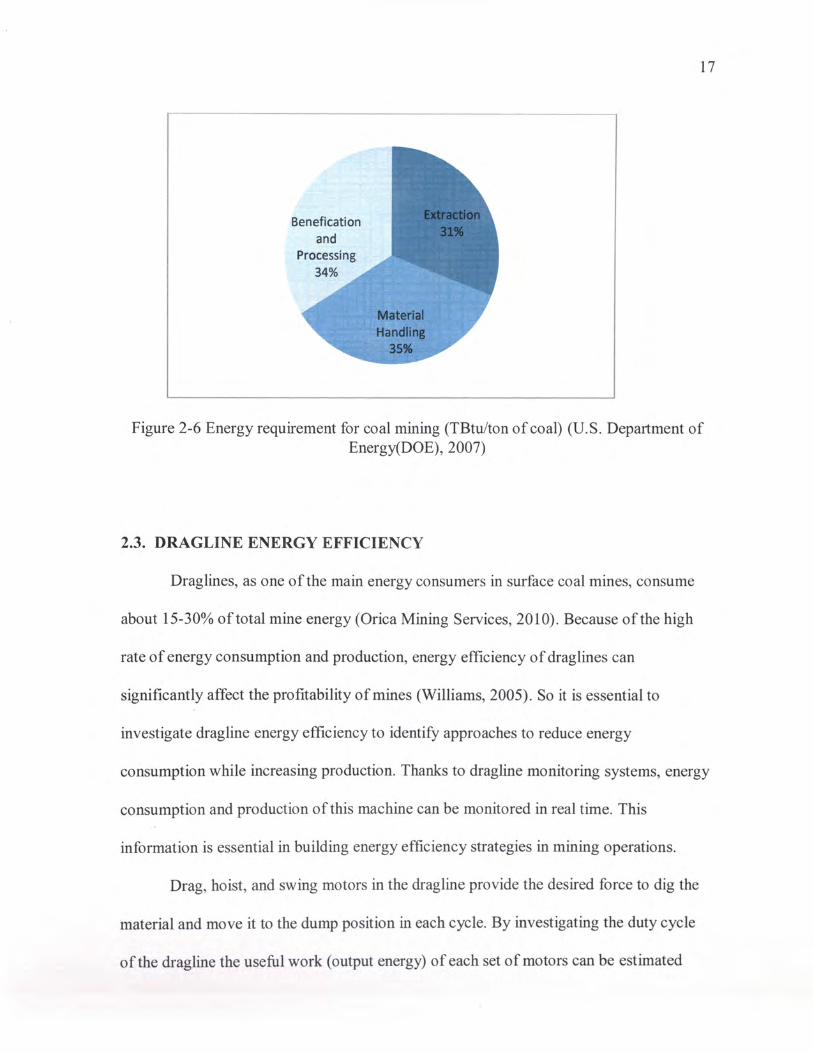
Generally, mining processes can be divided into three main stages; extraction,
material transportation and handling, and beneficiation and processing. Figure 2-6 shows
the share of energy requirement for each of these stages in coal mining, estimated by the
U.S. Department ofEnergy (DOE). Annual energy consumption of digging equipment
including hydraulic shovels, cable shovels, continuous mining machines, long-wall
mining machines, and draglines in coal mining industry is estimated as 7.7 billion kWh.
However, based on the DOE study, practical minimum energy required for digging

15
equipment in coal mines is 5.16 billion kWh. The DOE bandwidth analysis shows that
there is a potential of reducing the annual energy consumption to 169 billion kWh (579
Trillion Btu) which is about 46% of current annul energy consumption (U.S . Department
ofEnergy(DOE), 2007). The high potential for energy savings in mining has motivated
mining companies to identify opportunities for improving energy efficiency.
1400 .------------------
1200 -+------------------
1000 -+----------------·
Energy saving through -_______ ... Ill :::l efficiency gains ~ 800 -+---·------------c:
~ ·;:::: "C IV 600 1-----------::::::1 a
400
200
0 2000 2014
year
2040
Figure 2-5 World energy demand, adapted from (Exxon Mobil, 2013)

16
Energy costs account for 20 to 40 percent of typical mining operational costs
(Mielli & Wallace, 2012). Energy consumption is a key contributor to a business'
greenhouse gas emissions profile, which is currently voluntarily reported in the US (U.S.
Energy Information Administration (EIA), 2013), but may become compulsory in the
future. Improving energy efficiency in mining operations can reduce costs for energy,
increase profits and reduce emissions to meet government reporting requirements.
Efficient operations consume fewer resources for the same services or products (Dincer
& Rosen, 1999; Mielli, 2011; Steele & Sterling, 2011; World Energy Council, 2010).
An effective energy management system, that measures energy consumption to
identify energy saving opportunities and determines the relation between production and
energy consumption, is an important step to increase energy efficiency. Accurate
measurement of energy consumption is an important requirement for a successful energy
efficiency program. Limited information on energy consumption in mining operations is
one of the major challenges in identifying the best strategies to improve energy efficiency
(Bogunovic, 2008; Bush, Killingsworth, & Ruffel, 2002; Dessureault, 2007; Harney,
2007; Mielli, 2011).
Benefication and
17
Figure 2-6 Energy requirement for coal mining (TBtu/ton of coal) (U.S. Department of Energy(DOE), 2007)
2.3. DRAGLINE ENERGY EFFICIENCY
Draglines, as one of the main energy consumers in surface coal mines, consume
about 15-30% oftotal mine energy (Orica Mining Services, 2010). Because ofthe high
rate of energy consumption and production, energy efficiency of draglines can
significantly affect the profitability of mines (Williams, 2005). So it is essential to
investigate dragline energy efficiency to identify approaches to reduce energy
consumption while increasing production. Thanks to dragline monitoring systems, energy
consumption and production of this machine can be monitored in real time. This
information is essential in building energy efficiency strategies in mining operations.
Drag, hoist, and swing motors in the dragline provide the desired force to dig the
material and move it to the dump position in each cycle. By investigating the duty cycle
of the dragline the useful work (output energy) of each set of motors can be estimated

18
from engineering principles. Drag and hoist motors are mainly engaged in the digging
phase and elevating the material (Morley, Trutt, & Buchan, 1982). Eq. 2-1 describes the
work done by drag motors in each cycle.
Eout_drag = W drag_ bucket + W drag_ material + Wresistance + W friction 2-1
Where Eout_drag is the output energy of drag motors; W drag_ bucket is the work done to
drag the bucket; W drag_ material is the work done to drag the material; Wresistance is the work
done to overcome the resistance ofthe material to the cutting action; and Wrriction is the
work done to overcome the friction between material and the bucket.
The main duty ofhoist motors is to raise the material to the desired dumping
height. The useful work done by these motors can be written as in Eq. 2-2.
Eout_hoist = Whoist_material + Whoist_bucket + Whoist_chains 2-2
Where Eout_hoist is the output energy of hoist motors; Whoist_material is the work done
to overcome the weight ofthe material; Whoist_bucket is the work done to overcome the
weight of the bucket; and Whoist chains is the work done to overcome the weight ofthe
chains
Swing motors provide rotation of the machine from the digging to the dumping
position and return. The output energy of the swing motors can be calculated using
Eq. 2-3.

19
Eout_swing = Tswing X 8swing 2-3
Where Eout_swing is the output energy of swing motors; Tswing is swing torque; and
8swing is the angular displacement of the machine during the swing out and swing in.
Generally, energy efficiency is defined as the ratio ofuseful work done (energy
output) to the input energy (Zhu & Yin, 2008). In cases where either energy output or
input cannot be measured easily, proxy parameters are used in their place. Several
examples ofthis approach exist in the literature (Acaroglu, Ozdemir, & Asbury, 2008; K.
Awuah-Offei, Frimpong, & Askari-Nasab, 2005; K. Awuah-Offei et al., 2011; Cooley,
1955; Dupriest & Koederitz, 2005; Iai & Gertsch, 2013; Karpuz, C., Ceylanoglu &
Pa~amehmetoglu, 1992; Matuszak, 1982; Muro, Tsuchiya, & Kohno, 2002; Teale, 1965;
Torrance & Baldwin, 1990; Vynne, 2008). Vasilescu et al. (201 0) used work done in
carrying the payload from depth, d, for time, t, as a proxy for useful work done in their
work to design and control algorithms of an autonomous underwater vehicle capable of
missions of marine survey and monitoring (Vasilescu et al., 2010). Specific energy
(energy required to produce unit volume/mass of rock/soil) is widely used in excavation,
tunnel boring and soil cutting to measure efficiency ofthe excavation, boring, or cutting
process (Acaroglu et al., 2008; Muro et al., 2002). For instance, Muro et al. (2002) in
designing an experiment to estimate the steady state cutting performance, for varying
cutting depth for a disc cutter bit, used specific energy as the measure of performance
(Muro et al., 2002). Acaroglu et al. (2008) also used specific energy of a disc cutter for
predicting the performance ofTBM (Acaroglu et al., 2008). Specific energy has also been
used in drilling (Dupriest & Koederitz, 2005; Teale, 1965), shovel excavation (K.

20
Awuah-Offei et al., 2005; Karpuz, C., Ceylanoglu & Pa~amehmetoglu, 1992), and
ripping (lai & Gertsch, 2013). Specific energy is the inverse of energy efficiency, where
material produced (payload) is used as a proxy for energy output. Hence, higher specific
energy (or lower energy efficiency) is undesirable.
To fmd energy efficiency for loading and hauling operations, the amount of
material handled and fuel consumption are used as proxies for energy output and energy
input, respectively (Kwame Awuah-Offei, Osei, & Askari-Nasab, 2012). Dragline energy
efficiency can be defmed as the ratio oftotal weight of removed material to total energy
consumed to remove this amount of material (Eq.2-4).
. P tonnnes Energy Efficzency = 17 =-( )
E, kWh
2-4
Where Pis the payload and E1 is the energy consumption
2.4. DRAGLINE ENERGY MONITORING
A real-time monitoring system is an essential tool to reduce dragline energy
consumption. These monitoring systems can improve dragline performance and
productivity by displaying key performance indicators (KPis) such as payload, swing
angle, drag energy, cycle time, and its components. They also notify the operator when
the dragline is overloaded (payload exceeds recommended weight) or when certain alarm
conditions occur to reduce the maintenance cost. Providing operators with real-time
information helps them improve their performance and operate more efficiently (Vynne,
2008).

Prior to the 1980s, the mining industry was not motivated to conduct accurate
monitoring of dragline productivity because of the relatively smaller dragline sizes. At
that time, swing charts were used for collecting data manually. Tons of ore or coal or
overburden moved was used to describe dragline performance. However, these
parameters included the productivity of trucks, shovels and other material handling
systems as well as blasting performance into dragline performance (Cooley, 1955;
Matuszak, 1982).
21
In the 1980s, several different data loggers were developed; but it took time for
mining companies to realize the significant role these monitoring systems could play in
dragline monitoring. Data loggers are capable of reporting; total operating time,
productive operating time, machine motion performance, average swing angle, vertical
hoist to dump, average and maximum drag force, average bucket load, average maximum
lowering and payout speeds, etc. (Matuszak, 1982).
Tritronics 9000 Monitor is one ofthe oldest and most popular monitoring systems
and was first developed in 1983. Several technical challenges, such as proper detection of
all the different facets of dragline operation, strong computational power to convert all
the measured values to meaningful metrics and the ability to be left unattended while
collecting and storing data for later analysis, were solved to build this monitoring system.
It had an onboard computer for monitoring dragline operation and radio telemetry to
transfer the data to an offboard computer for storing and analyzing. The onboard
computer logs armature voltage and current of drag, hoist, and swing motors; swing
angle; hoist and drag rope length; position of drag and hoist master switches; indication
of propel mode; and number of steps in the walking process. This data is necessary for

22
quantitative measurements of production in each cycles and real-time analysis ofbucket
position. Operators logged in the digging modes and delay codes into system manually.
Parameters such as total number of swings since the shift began and the running total of
material moved were displayed for the operator via a digital readout. These inputs were
then converted into a record for each cycle, stored, and transferred into to the mine office
computer (Hawkes, Spathis, & Sengstock, 1995; Torrance & Baldwin, 1990).
These days several manufacturers produce different real-time monitoring
systems. Each uses a different method to evaluate the key parameters and operator
performance. AccuWiegh™ by Drives & Controls Services (DCS) and Virtual
Information Management System (VIMS) by Caterpillar® are other monitoring systems
that use raw data from the dragline and convert it into meaningful information with
supplied software. The data is then stored in different databases, using software such as;
MS Access, MS SQL, MySQL, and Oracle, for further analysis (Bogunovic et al., 2009;
Drives & Controls Services, 2003; Komljenovic et al., 2010).
A dragline monitoring system collects and stores different sets of parameters in
each cycle depending on the system set up and metrics. Monitoring dragline operation for
even a short period will result in a big data set. This data can be a great source for
assessing useful metrics such as productivity, dragline performance for different
operating conditions or tasks, and operator performance, as well as help identify the best
strategies to improve energy efficiency. However, only a small portion of the collected
information contributes to useful results, because of data overload and absence of post
processing software (Morrison & Scott, 2002). Despite the high potential of monitoring
systems to contribute in these analyses, not enough attention has been paid to analyzing

the data collected and post processing analyses by dragline monitoring systems
(Hettinger & Lumley, 1999; Morrison & Scott, 2002).
2.5. FACTORS AFFECTING DRAGLINE ENERGY EFFICIENCY
Eq. 2-4 implies payload or productivity and energy consumption are key
parameters that control dragline energy efficiency. In order to manage dragline energy
efficiency, it is essential to identify factors that affect dragline productivity and energy
consumption. This section provides a summary of previous work done to recognize
factors that affect energy consumption and productivity.
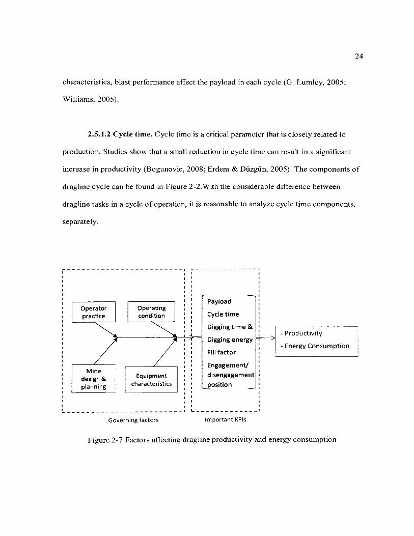
Payload, cycle time, digging time and energy, fill factor, engagement and
disengagement position are important KPis, which are closely linked to dragline
productivity and energy consumption (Figure 2-7). These parameters are controlled by
four main governing factors; operating condition, mine design and planning, equipment
characteristics, and operator's practice (K. Awuah-Offei et al., 2011; Bogunovic &
Kecojevic, 2011; Hettinger & Lumley, 1999; Kizil, 2010; G. Lumley, 2005).
23
2.5.1. Important KPis. Important KPis significantly affect dragline productivity,
energy consumption, and, consequently, dragline energy efficiency. These parameters
have been used in previous studies to assess dragline performance metrics such as
productivity and operators' performance.
2.5.1.1 Payload. The results ofthe correlation analysis between dragline KPis
and productivity shows that payload has a strong relation with dragline productivity.
Factors such as bucket design, material properties or geology, operators' skill, motor
24
characteristics, blast performance affect the payload in each cycle (G. Lumley, 2005;
Williams, 2005).
2.5.1.2 Cycle time. Cycle time is a critical parameter that is closely related to
production. Studies show that a small reduction in cycle time can result in a significant
increase in productivity (Bogunovic, 2008; Erdem & Diizgiin, 2005). The components of
dragline cycle can be found in Figure 2-2.With the considerable difference between
dragline tasks in a cycle of operation, it is reasonable to analyze cycle time components,
separately.
Operator practice
Mine design& planning
Operating condition
Equipment characteristics
-Payload
Cycle time
Digging time &
Digging energy • /
Fill factor
Engagement/
disengagement
position
~------------------------ L-------------Governing factors Important KPis
- Productivity
- Energy Consumption
Figure 2-7 Factors affecting dragline productivity and energy consumption

25
2.5.1.3 Digging time and digging energy. Many authors have found the digging
phase the most critical component in dragline cycle with the highest impact on energy
consumption and production rate. Different digging conditions such as digging near cut
walls, cut bottom or key cutting can significantly increase dig time. Dig time can be
reduced by proper bench blasting and proper angle of attack between the bucket teeth and
the ground, which is controlled by operator (Bogunovic & Kecojevic, 2011; Erdem &
Diizgiin, 2005; Rai, Ratnesh, & Nath, 2000; Rai, 2004; Torrance & Baldwin, 1990;
Williams, 2005). Bogunovic (2008) used the energy consumption of just digging phase to
evaluate operator performance (Bogunovic, 2008). Bogunovic (2011) concluded that dig
time is the only cycle time component that is influenced by operator performance
(Bogunovic & Kecojevic, 2011). The weakness ofthese assumptions and conclusions is
that they are made without considering other phases in the dragline operation cycle.
2.5.1.4 Fill factor. Bucket fill factor is found as a parameter that influences
production rate and energy consumption. Eq. 2-5 shows the defmition of bucket fill factor
FF= PxSF BVxMD
2-5
Where; FF is fill factor, W is payload, SF is swell factor, BV is volume of bucket,
and MD is material density.
The best fill factor for a given dragline should maximize payload and minimize
dig energy consumption. This factor is controlled by operator skill and performance.
Blast performance and material properties can also affect the dig energy consumption. A

26
study done on a Marion 8200 dragline, with the bucket capacity of82 yd3, indicated that
the optimal bucket fill factor (78%) reduces electricity used in digging phase by 36% and
improve production rate by 1.4% (Bogunovic & Kecojevic, 2011; Bogunovic, 2008).
2.5.1.5 Engagement/disengagement position. Specific functional analysis done
by Hettinger and Lumley (1999) shows that bucket engagement position, which is
influenced by mine plan and operator habit, affects dragline productivity. For each bucket
and rigging system there is a particular disengagement position at which payload is
maximized. Disengage positions away from this optimum point result in payload spillage,
increased cycle time and loss ofproductivity (Hettinger & Lumley, 1999).
2.5.2. Governing Parameters. Governing parameters are parameters that control
important KPis and consequently dragline production, energy consumption and energy
efficiency.
2.5.2.1 Operating conditions. Operating conditions, such as geology, material
properties, groundwater level, and weather condition, are known to be controlling
parameters. Each mine has its own operating condition, which makes the size ofthe
mine, mine plans and equipment selection unique for that specific mine. Based on the
operating conditions of a mine, dragline performance can vary, significantly (Bogunovic
& Kecojevic, 2011), (Rai et al., 2000), (Bogunovic, 2008). Operating conditions are not
changeable so mine designs should be compatible with these conditions to get the
maximum efficiency.

27
2.5.2.2 Mine design and planning. Digging method, mine strips and dumping
position affect swing angle, swing time, and, consequently, cycle time. An optimum mine
design should assign tasks to the dragline in proper timing to maximize mine productivity
and keep energy consumption, maintenance cost, and wasted time minimum. Assigning
inappropriate tasks, such as deep cuts, to dragline can increase energy consumption and
make the operation inefficient (Erdem & Diizgiin, 2005; Rai et al., 2000). For example,
Pippenger (1995) showed that changing dragline shift from seven-day, three-shift, eight
hour to two 12-hour shifts per day reduces lost operational times and increases
productivity (Pippenger, 1995).
2.5.2.3 Equipment characteristics. An appropriate bucket size, sufficient motor
power, and proper gear ratios can increase dragline productivity and reduce energy
consumption (Pippenger, 1995), (Rowlands & Just, 1992).
In cases where a mine purchases used draglines, the bucket size and drive system
may not be completely compatible with the operating condition. Thus, some
modifications may need to be done on draglines. However, modifying dragline drive
system or bucket is costly. In Australia, during 2003 and 2004, about $30 million was
spent on UDD (Universal-Dig-Dump) conservation: more than $20 million on new
buckets, boom upgrades, and electrical upgrades, etc. (G. Lumley, 2005).
2.5.2.4 Operators practice. Operators' skills and habits have been observed to be
important factors affecting dragline KPis, productivity, and energy consumption. An
operator's practice and skills are mostly measured by his/her performance and

28
productivity. Due to the important role of drag lines in mine profitability, assessing
operator performance is an important issue. Australian coal mines became more
profitable and efficient after the structural changes in their hiring policy in 1997. As a
major part of this, mines now have the ability to select operators and employees based on
their performance rather than seniority. Lumley (2004) detected the average difference of
35% between productivity of the best and the worst operator in GBI database (G. I.
Lumley, 2004; G. Lumley, 2005). Dragline productivity varies greatly between operators,
even in the same operating condition (K. Awuah-Offei et al., 2011; Bogunovic et al.,
2009; Bogunovic, 2008; Komljenovic et al., 2010; Norman, 2011; Patnayak et al., 2007).
Dragline production has always overshadowed dragline energy efficiency. The objective
function of most ofthe studies described in this section is to maximize dragline
productivity. However, with the growing concerns about reducing energy consumption
and improving energy efficiency more investigations need to be carried out on dragline
energy consumption and efficiency to help mining companies increase their productivity
whilst keeping their energy consumption and energy cost reasonable.
Of all the factors that affect dragline productivity and energy efficiency, operator
skill and performance is, probably, the most inexpensive factor to change. Operating
condition, mine design and planning, equipment characteristics and operators' skill are
factors that control dragline productivity, energy consumption and efficiency. In a given
mine, maximizing energy efficiency by changing operating condition is not possible.
Also optimizing dragline drive mechanism can be costly. Mine design should not assign
tasks to dragline in which its efficiency is low. But some ofthese circumstances are
unavoidable, for instance digging near cut walls, cut bottom or a key cutting. Operators

29
can be trained to improve their performance and increase productivity. Training operators
is a relatively cheap improvement and valid approach in comparison to other
modifications. To train operators, it is critical to understand the effect of operators
practice on dragline productivity, energy consumption and energy efficiency and quantify
this relationship.
2.6. ASSESSING THE EFFECT OF OPERA TOR'S PRACTICE
The importance of operator performance for profitability highlights the
significance of an operator performance assessment system. Multiple criteria have been
used to assess operator performance for different equipment in different industries.
Parameters such as course, altitude, speed, timing, and handling are used to assess the
performance of pilots in a flight simulator test in each flight task. These single dimension
values are then combined for evaluating the fmal score of each pilot (Johannes et al.,
2007). For haul trucks, operator training and performance evaluation focuses on
improving productivity, reducing maintenance cost, and improving safety (Vista, 2013).
Patnayak (2007) suggested using hoist energy consumption per tonne of material
excavated and number of required cycles to load a truck to assess operator performance
and productivity. He also used the one-way analysis of variance (ANOVA) to test the
hypothesis that the mean of hoist and crowd power between operators are equal in
electric shovels. The results ofthese tests indicated that hoist power is significantly
different between operators at a significance level ofO.Ol (Patnayak et al., 2007).
Although, the ANOV A test is a common and valid approach to compare the mean
between more than two groups, comparing the hoist power alone without considering the
30
productivity, is limited as a measurement of performance of different operators. In cases
where crowd and swing energy are significantly different, the inferences may be
misleading.
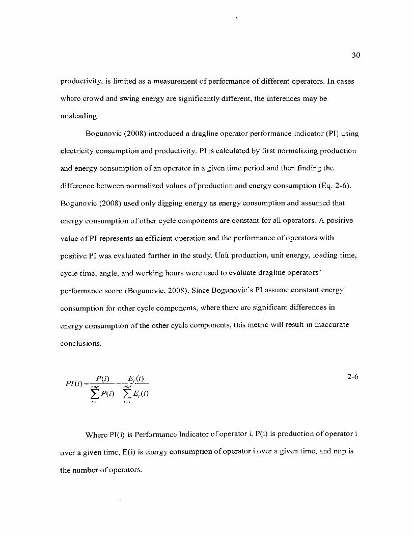
Bogunovic (2008) introduced a dragline operator performance indicator (PI) using
electricity consumption and productivity. PI is calculated by first normalizing production
and energy consumption of an operator in a given time period and then finding the
difference between normalized values of production and energy consumption (Eq. 2-6).
Bogunovic (2008) used only digging energy as energy consumption and assumed that
energy consumption of other cycle components are constant for all operators. A positive
value of PI represents an efficient operation and the performance of operators with
positive PI was evaluated further in the study. Unit production, unit energy, loading time,
cycle time, angle, and working hours were used to evaluate dragline operators'
performance score (Bogunovic, 2008). Since Bogunovic's PI assume constant energy
consumption for other cycle components, where there are significant differences in
energy consumption of the other cycle components, this metric will result in inaccurate
conclusions.
PI(i)= P(i) nop
:LP(i)
2-6 nop
:LEJi) i=l i=l
Where PI(i) is Performance Indicator of operator i, P(i) is production of operator i
over a given time, E(i) is energy consumption of operator i over a given time, and nap is
the number of operators.

31
Komljenovic et al. (2010) presented an operator performance indicator (OPI) that
specifically evaluates dragline productivity and energy consumption. OPI was defmed as
the dragline production over the dragline energy consumption in a given period of time
(Eq. 2-7). Different confidence intervals were used to create a classification system to
evaluate operators' performance based on OPI. Assuming that OPI follows t-distribution
(when number of operators are less than 30), Eq. 2-8 was used to defme the boundaries of
the classification system (Komljenovic et al., 2010).
OPI(i)= P(i) E(i)
Where OPI(i) is the Operator Performance Indicator of operator i
s OP/upper;lower =OP/s±ta. C
2,nop-l vnop
2-7
2-8
Where OPI upper;Iower is OPI boundaries, OPis is sample mean, Ss sample standard
deviation, tu~2;nop-J is the 1 OOa./2 percentage point of the Student distribution with (nop-1 ).
Bogunovic (2008) and Komljenovic et al. (2010) used single performance criteria
over a period. This prevents analysts from tracking the effect ofvariations in control
variables over the period of evaluation. In cases where such control variables vary
significantly over the evaluation period and between operators, wrong conclusions can be
made about operator performance. It is important to monitor variables that significantly
affect operator practice during performance assessment. Knowing which of these

32
variables are significantly different between operators with different performance
metrics, can help us to improve training systems. Intuitively, this approach is the basis for
crew coaching in many mines. For example at the Coal Creek Mine, a leader operator
(expert operator) spends time watching and evaluating oiler/groundman (operator with
less experience) and provides him/her with feedback to increase his/her performance,
based on observed sub-optimal practices (Norman, 2011).
2.7. SUMMARY
Improving energy efficiency is a cost-effective approach to meet the increasing
demand of energy whilst reducing environmental impacts of energy consumption.
Productivity and energy efficiency of the dragline, as a dominant machine in surface
mines, have a great impact on mine profitability. The real-time monitoring systems on
draglines provide us essential information to build energy efficiency strategies in mining
operations. Energy efficiency of dragline can be defmed by using payload and total
energy consumption as proxy parameters for useful work and input energy, respectively.
Identifying factors that affect dragline productivity and energy consumption is
essential to manage dragline energy efficiency. Key performance indicators, which are
closely linked to dragline productivity and energy consumption, include payload, cycle
time, digging time and energy, fill factor, engagement and disengagement position. Four
governing factors; operator practice, operating conditions, mine design and planning, and
equipment characteristics control these KPis. Among these governing factors operator
performance is the most inexpensive factor to modify in order to maximize energy
efficiency. In a given mine changing operating condition is not always possible,

33
optimizing dragline drive mechanism can be costly, and sometimes it is unavoidable to
assign inefficient tasks to dragline. Training operators to improve their performance can
be a relatively cheap improvement and a valid approach to improve energy efficiency.
It is critical to understand the effect of operator practice on dragline energy
efficiency and quantify this relationship. Identifying variables that are significantly
different between operators with different performance can help us to improve training
systems.

34
3. FIELD DATA ACQUISITION FOR CASE STUDIES
3.1. STUDY SITE
The methods presented in this work are illustrated with data from a real mine. The
data was collected from a mine 1 located in the Powder River Basin (PRB) in Wyoming.
PRB covers 20,000 mile square in north-central Wyoming and south-east Montana. It is
recognized as a valuable source of coal bed methane, coal, petroleum, conventional
natural gas and uranium oxide (United States Environmental Protection Agency (EPA),
2004).
3.1.1. Geology. PRB is a thick sequence of sedimentary rock ranged from
Paleozoic through Mesozoic and Tertiary. Paleocene Fort Union and Eocene Wasatch are
two formations in PRB containing coal beds (Wyoming State Geological Survey, 2010).
Wasatch formation covers 1/3 ofPRB and contains mostly continuous and thin (6
feet or less) coal beds with high heat values and agglomeration characteristics (United
States Environmental Protection Agency (EPA), 2004; Wyoming State Geological
Survey, 2010). Coal deposits in Fort Union formation are identified as the thickest and
most extensive deposits of low-sulfur subbituminous coal in the world and are mostly
formed in the upper Tongue River Member (United States Environmental Protection
Agency (EPA), 2004). They range from subbituminous C to A in apparent rank, in the
shallow part ofthe basin (surface to 1,000 ft. of depth) low rank coal (subbituminous C)
can be found. Middle rank coal (subbituminous B) and high rank coal (subbituminous A)
1 To protect the mine's identity no name will be used in this thesis.

are placed in intermediate depth (1,000 to 1,400 ft.) and deeper part ofthe basin (more
than 1,400 ft.), relatively (Stricker et al., 2007).
35
The average energy content in the PRB coal is 8,500 Btu/lb with low sulfur
content. Considering that the average energy content of coal produced in the U.S. in 2011
was nearly 9,800 Btu/lb., PRB coal has a low energy content (U.S. Energy Information
Administration (EIA), 2012). However, the low sulfur content enables power plants to
burn the PRB coal with no need for expensive emissions control equipment, which makes
PRB coal economic to extract ("PRB Coal Properties," 2013). The share ofthe coal
production from PRB was 37% of total coal production in the U.S. in 2011 (United States
Environmental Protection Agency (EPA), 2004).
US Geological Survey (USGS) (2008) divided PRB into three regional areas.
Gillette coalfield is the most significant area (covers about 2,000 mile squared); known as
the most prolific coalfield in the U.S. In 2006, nine out often largest coal mines were in
this coalfield. Tongue River member supply the 13 active mines operating in Gillette
coalfield, including the understudied mine (USGS, 2008). Figure 3-1 displays the
stratigraphy of coal in this coalfield. The Ronald coal bed, with the average thickness of
lOft, is the boundary between Wasatch and Fort Union formation. The maximum
thickness ofthis coal bed and maximum overburden are 52 ft. and 1,175 ft, respectively.
The mine extracts coal from this coal bed. The two main seams in this mine are Roland 1
and Ronald 3 with the average energy content of8,226 Btu and 5.67% of ash (USGS,
2008).

36
3.1.2. Mine Operations. Construction in the mine started in spring 1979 and the
first coal was shipped in May 1982. As at December 2011, the recoverable reserve is
estimated at 175.4 million tons (Arch Coal Inc., 2012).
Formation Bed name Average thickness
Wasatch
Figure 3-1 Coal stratigraphy in the Gillette coalfield (adapted from (USGS, 2008))
The total coal production of the mine in 2011 was about 11.4 million tons.
Average thickness of coal seams Roland 1 and 3 are 26 feet and 13 feet. The two seams
are separated by a thin interburden. Mining is done by strip mining with truck and shovel
pre-stripping. The average thickness of overburden is 90 feet. In places where the

37
thickness of overburden exceeds 1 00 feet shovels and trucks are used to clear the
overburden until an overburden thickness of 1 00 feet. The remaining 1 00-foot
overburden is removed with a Bucyrus-Erie 1570W dragline with a bucket capacity of 85
yd3.
The drag line is equipped with Accuweigh ™ monitoring system (by Drives &
Control Services 2) that collects raw machine signals, converts them to meaningful
parameters in each cycle and stores them in a database (Drives & Controls Services,
2003). The relevant parameters in the database were retrieved from the database for this
study. Table 3-1 shows the operating specifications ofthe dragline. Figure 3-2 displays a
typical mining sequence at the mine. Figure 3-3 shows the configuration of the dragline
drive mechanism and the list ofthe dragline's electrical drive components (motors and
generators) is displayed in Table 3-2.
3.2. FIELD EXPERIMENT
The field experiment involved a site visit, monitoring the dragline for one month
during which different operators run the machine under similar conditions, and data
retrieval for research. The mine visit (which was on June 19th and 201\ 20 12) involved
visiting the mine site, and surrounding area, and observing the dragline operation under
study and two other draglines in another mine in the area. The author observed working
draglines with different operators, operator habits, different operating conditions, and
dragline drive components, which helped to better understand the collected data.
2 http://www.drivesandcontrols.com/

Quantity
2
2
6
4
4
4
Table 3-1 Operating specifications of a Bucyrus-Erie 1570W drag1ine
Parameter Value
Clearance radius (Rear end) 21.4 m
Operating radius 87.5m
Boom length 99.1 m
Boom angle 38°
Clearance height (under frame) 2.4m
Tub Diameter 20.1 m
Dumping Clearance 45.7m
Boom point height 65.2m
Maximum digging depth 53.3 m
Width (shoe-shoe) 28.0m
Rated suspended load 176 tonnes
Step length (approx.) 2.6m
Table 3-2 Electrical configuration of dragline motors/generators
Motors/ Generators
2000 HP- 4 unit MG sets (Motor generator sets)
3000 HP- 5 unit MG sets (Motor generator sets)
1300 HP hoist motors
1300 HP drag motors
I 045 HP swing motors
500 HP propel motors
38

39
-- -----v
~
100ft.
Figure 3-2 Mining sequence in the mine

'
DRAG DRUM
~~~ rMl~ ~
~--~
HOIST DRUM
g·~IM~~ 0 0 0 0
Figure 3-3 Schematic representation of drag line drive
~Q -,: \)~'';/
1b~wil.J.:
~----'
16 )wi~'~_':, ~- ~n~t_,'
~-----, ~"-'i,,e- '
'' _ll~;~ - -
~ 0

41
The data used in this work was collected during one month (June 18th to July 18th,
2013). Accuweigh™ monitoring system was used as a remote observation tool. Such
micro-processor based data acquisition is cheaper (no labor costs), comprehensive (data
capture is continuous throughout the experimental period), and more accurate as human
errors are removed or minimized in the data collection. Accuweigh™ monitoring system
provides the operator with information such as position of the bucket on a map on the
digital screen, payload, swing angle, etc. in a real time. The monitoring system also keeps
track of over loading the machine and warns the operator. Not all the recorded parameters
are displayed to the operators, but they are all stored in the main data base. In order to
fully capture energy efficiency, there is a need to monitor the components of energy
consumption during a dragline cycle- drag, hoist, and drag energy. Since Accuweigh ™
does not store this data in the database, this work involved modifying the program to
store this data in the extra database fields of the database. The main data base also
contains information from shovels, trucks, draglines, etc. in separated tables. Information
such as operator's JD number, dragline activity code, operating shift and pit are recorded
in separate tables. By matching records in this table with records in the dragline table, the
author was able to verify that during the period of data collection the drag line worked in
the West Pit with thirteen different operators. The dragline activity during this time
included digging below grade (84.7 %), rehandling (15%), and other activities (0.3%).
The average recorded temperature during this time was 74°F.

42
3.3. SUMMARY
Data collected from a real mine was used in this work to illustrate the presented
methods. Data was collected from BE-1570w dragline with bucket capacity of85 yd3
equipped with Accuweigh™ monitoring system during one month. Some modification to
the program was necessary to store drag, hoist and swing energy in the database. The
main duty of the dragline in this mine is to remove the overburden (with average
thickness of90 ft.) from the coal seams. It is assumed that during the data collection the
material type remained constant as the dragline was operating in one pit. During this time
dragline spent 84.7% of its time for digging below grade, 15% rehandeling, and 0.3% for
other activities.

43
4. PRELIMINARY DATA ANALYSIS OF FIELD DATA
This section contains preliminary data analysis of the field data, which is used to
illustrate the methods formulated in this research. The preliminary data analysis is helpful
for studying the structure and behavior of the field data prior to analysis. In this section
the data collected from a Bucyrus-Erie 1570w (85 yd3 bucket) using Accuweigh™
monitoring system is studied graphically and quantitatively using SQL server
management studio (Microsoft, 2008), MATLAB, and SAS.
4.1. STRUCTURE OF DATASET
The dataset used in this study was retrieved from the main dragline monitoring
database of the mine. In one month 34,326 cycles were recorded. Each cycle contains 44
parameters regarding the working positions, time spent on the cycles and portions of
cycles, swinging angles, dumping heights, and energy consumed by drag, hoist and swing
motors (a list of all44 parameters and their defmitions are included in APPENDIX A).
The Accuweight TM monitoring system is designed to collect the total time spent on each
cycle and the tasks carried out in each cycle, separately. A cycle is defmed to start when
the last load was dumped and end when the current load is dumped. Components of a
cycle are swinging out, dumping, swinging in, spotting and loading (Figure 4-1 ).
Swinging out time is measured as the time elapsed from the moment the bucket is
detected to be full to the time it is detected to be empty. Dumping time is the time
between when the bucket is in the dump zone to when the bucket is detected as empty.
Swinging in time is the time between when the bucket is dumped and when a dig detect is
triggered. Spotting time is measured from the moment the swing velocity is less than a

given value to the moment when the dig detect is activated. The time between when the
bucket fill is detected and full hoist is detected is defmed as loading time.
Fill t:. .... --:> Hoist Bucket Bucket
II \ Spot
Bucket Swing
out
/) Swing in Dump (Return) ~ material
Figure 4-1 Dragline cycle components
Not all the 44 parameters recorded in the dataset were relevant to this work.
Fourteen parameters adjudged to be useful for studying dragline energy efficiency were
retrieved from the main database for further analysis. Table 4-1 shows a brief summary
ofthese parameters.
44

Swing out
Parameters time
Units Milliseconds
Minimum 1500
Maximum 2500
Mean 2.05e+4
Variance 5.17e+6
Parameters Angle swing
out
Units Degree
Minimum 1
Maximum 384
Mean 61.73
Variance 838.83
Table 4-1 Relevant Parameters
Load bucket
Swing in time time Dump time Cycle time
Milliseconds Milliseconds Milliseconds Milliseconds
13000 6000 6000 41000
34000 16000 13000 70000
2.15e+4 1.08e+4 9.1le+3 5.40e+4
1.97e+7 6.16e+6 1.74e+6 4.29e+7
Drag Drag
distance distance Dump height Drag energy
(horizontal) (vertical)
Inch Inch Inch Kw-s
0 -466 235 -7491
837 980 2299 20971
138.94 138.43 1.02e+3 3.25e+3
12267.66 18372.49 1.54e+5 3.44e+7
Spot time
Milliseconds
1000
16000
8.28e+3
6.98e+6
Hoist energy
Kw-s
14299
54859
3.23e+4
8.63e+7
Payload
Pounds
337833
501283
4.29e+5
1.12e+9
Swing
energy
Kw-s
1570
21065
6.6e+3
7.43e+6
.j::.. VI

46
The data was first classified based on the number of attempts operators made to
fill the bucket. In the majority (about 98%) of cycles, the operator successfully filled the
bucket on the first attempt {Table 4-2). All the cycles which took more than one attempt
were ignored in this study (some of these could be highwall chopping operations)
because they did not represent "normal" loading operations. APPENDIX B contains raw
data used in this work.
Table 4-2 Classification ofthe data based on number ofbucket reloads
Bucket Reload Count Proportion (%)
0 33,492 97.56
1 738 2.15
2 53 0.15
3 or more 43 0.13
4.2. DETECTING AND REMOVING OUTLIERS
Outliers must be removed prior to any analysis in order to prevent inaccurate
inferences. In this research, outliers arise from errors (values recorded during periods
when the dragline is not operating etc.) and anomalous operating cycles. The fourteen
parameters were examined for outliers. A common approach to detect outliers is to
determine the first (Q1) and third quartiles (Q3) and calculate the interquartile range using
Eq.4-1.
4-1

47
The points that are outside the quartiles by one and a half IQR (lower and upper
Whisker) are labeled as mild outliers. Boxplots are commonly used to display the outliers
graphically. In Figure 4-2 red crosses represent the outliers.
25%
25%
25%
25%
+
+ --------· Outlier + +
+
Upper whisker
Quartile group 4
------- Upperquartile
Quartile group 3
------- Median
Quartile group 2
_____ .Lower quartile
Quartile group 1 _ _ _ _ _ _ _ Lower whisker
Figure 4-2 Boxplot definition in this work
MATLAB was used to plot the boxplots of the fourteen parameters in the
database (Figure 4-3). Figure 4-4 shows the boxplots after removing mild outliers. Note
that new "outliers" are identified because the statistics (Q,, Qz, and IQR) have changed
with the new data set (i.e. data without the original outliers).

48
4.3. DRAGLINE OPERATORS
During the one month of data collection, thirteen different operators operated the
dragline. Table 4-3 shows the operating time and number of cycles for each operator. It is
essential to have equal support from all operators in the analysis to make reasonable
inferences. Not all operators worked sufficient amount of hours to be considered in the
statistical analysis.
Table 4-3 Operator activity
Operator #of cycles Total operating time (hr)
3,897 56.91
B 3,611 54.62
c 3,350 49.60
D 3,058 45.64
E 2,211 32.77
F 1,529 23.55
G 1,023 15.70
H 761 12.39
I 271 4.36
J 129 2.04
K 88 1.09
L 29 0.49
M 24 0.35

X 104 X 104 x 1 o• X 104 X 105 X 104
10[ + hol '*' ~ 1 or '*'
~ 10 [ + ~ sf '*'
~ 10t
Sf 1 8
I 8 8 4 :j: 8
+
'*' Sf 4; + +
6 6 6 3
j 6
+
4 f 4 4
t 2 4
4 I
2 f I 2 2 1 2
B I 2 E¥3 = T 9 0 ...!... 0 l 0 0 0 +
Swing out t(ms) Swing in t(ms) Load bucket t(ms) Dump t(ms) Cycle t(ms) Spot t(ms)
X 105 X 104 x 1 o' 4001 8
t I + 4
' + 10 +
2500
I + 1000
I 6 l 3.5 I
I 8
300 f
I 500 2000 I
I I 3 B 4 6 I
0 B 1500 I I
200 f
! I 2.5 4
I I B I I 2 -500 1000 I 2 I I
I 8 I I 2 I
100 f I -1000 8 I 1.5 0
~ 500 I I 0 I -1500 I 1 i Of ...!...
'*' 0 _I_ -2 -2
1 1 1 1 1 Swing angle(deg) Drag dis v(in.) Drag dis h(in.) Payload(lb) Drag en (kW-s) Hoist en (kW-s)
Figure 4-3 Boxplots of relevant parameters before removing any outlier
2500 • I
2000 I I I
1500 I
8 1000
500 I I I 0 I
.!..
Dump height(in.)
X 104
I 3
2
I 1 I
8 I
0 ! +
Swing en (kW-s)
..j::.. \0

2 .8
2 .6
2 .4
2 .2
2
1 .8
1.6
X 104
I I I I I I I I
~ I I I I
.!.
X 104 5
4
3
2
I I I I I I
B I I
_I_
I ~
I
!
X 104
+ +
T
I
2 ~ + 12000
I
+ I I
T I
I
I I
I I
1 . 5 ~ I 10000 I
I
~ I
H 8 8000 I I
I I I I I - 6000 .!.
., 1 -,- 1
X 104
+
9 ~ I 8 ~ I I
n I I I I
6 ~ 8 5 ~ I I
4 I -
Swing out t(ms)Swing in t(ms)Load bucket t(ms) Dump t(ms) Cycle t(ms)
X 105 500
I • 1600
' 3 .5 T 20000 T
200 ~ I I
400 I
I I I I 1400 I I I I
I I 15000 I I I I I
150 ~ 300 I 1200 I 3
~ I
I I 10000 I
I I I I I 1000 I
~ I 200
~ ~ 100 ~
I 5000 I 800 2.5 I I
8 100 I
600 I 0 I 50 ~ 0 I I I I
I 400 I I I I I I 2 I -5000 I I I I + I - -100 - 200 - -.,
I I I
X 104
+ 2000 I
2 .5 t I I
t I I
2 + I + 1500 I t I
I I 1.5 I
~ I I
1000 1 ~ 0 .5 I
I I I 500 I I I
0 - -1
Spot t(ms) Dump height(in .)
X 104 X 104
T
I I 2 5 I
I I I I 1.5
4 I
~ I I I
1 I 3 I
B I I 0 .5 2 I I I I I I - -I
Swing angle(deg)Drag dis v(in.) Drag dis h(in.) Payload(lb) Drag en (kW-~ist en (kW-s)Swing en (kW-s)
Figure 4-4 Boxplots of relevant parameters after removing outliers
Vl 0

51
The mean standard error of energy efficiency of each operator was calculated
using Eq. 4-2 (Biau, 2011). The gradient of the standard error increased after operator H
(Figure 4-5). Operators with mean standard error greater than 0.06 were removed from
the database. Figure 4-6 displays the mean standard error and the number of cycles of
eight operators. The increase in gradient of the standard error after operator D shows a
change in the mean standard error. Because ofthe sudden change the mean standard error
of operator D can be used as a cut-off value. Operator E was also included in the analysis,
based on the author's engineering judgment, to increase the number of operators in the
analysis while maintaining reasonable confidence in estimates ofthe mean energy
efficiency. Thus, 0.04 was chosen as the cut-off value to fmd the minimum required
number of cycles.
-+-Standard error ..... Cycles
0.35 .,....-------------------, 4,500
+IL:----------------J'-\------1 4,000 0.3
A B C D E F G H
Operator
K L M
3,500 Ill
Cll
3,000 ~ u
2,500 '0 2,000 ]
1,500 § 1,000 z 500
0
Figure 4-5 Mean standard error and number of cycles of all operators

....
0.07
0.06
e (jj 0.05
"C :; 0.04
"C r:: ~ 0.03 Ill
r:: ~ 0.02 ~
0.01
-.-standard Error - Number of cycles
4,500
4,000
3,500 Ill
Cll
3,000 ~ u
2,500 0
t-~~~.----.----~~--~~-------------1 2,000 ~ 1,500 § 1,000 z 500
0 +----.----~---,r---~----~--~----~---+ 0 A B c D E F G H
Operator
Figure 4-6 Mean standard error and number of cycles of eight operators
52
It can be concluded from Table 4-4 that operators with number of cycles less than
2000 have the relatively high standard error (greater than 0.04). Operators A, B, C, D,
and E with standard error less than 0.04 were included in the analysis.
SE = _!!j_ ' nOc;
4-2
Where SEi is the mean standard error of operator i energy efficiency; cri is
standard deviation of operator i energy efficiency; nOci is number of cycles of operator i.
4.4. SUMMARY
Preliminary data analysis in this work included; investigating the structure of the
data; removing the outliers; and identifying operators with sufficient working hours to be

53
considered in further analysis. Cycles in which the bucket was not filled successfully in
the first attempt were removed from the data since they did not represent normal loading
operation. Mild outliers were removed to reduce the chance of drawing wrong inferences.
Five operators with standard error of mean of energy efficiency less than 0.04 were used
for further analysis.
Table 4-4 Standard error
Mean Standard
Time energy deviation energy Standard
Operator #of cycles (hours) efficiency efficiency error
A 3,897 56.91 5.31 1.680 0.027
B 3,611 54.62 6.06 1.712 0.028
c 3,350 49.60 6.26 1.707 0.029
D 3,058 45.64 6.34 1.680 0.030
E 2,211 32.77 6.41 1.686 0.035
F 1,529 23.55 6.47 1.700 0.043
G 1,023 15.70 6.49 1.707 0.053
H 761 12.39 6.55 1.712 0.062
I 271 4.36 6.82 1.712 0.104
J 129 2.04 6.88 1.755 0.154
K 88 1.09 7.19 1.733 0.184
L 29 0.49 7.24 1.756 0.326
M 24 0.35 7.29 0.671 0.137

5. EFFECTS OF OPEARTOR PRACTICE ON DRAGLINE ENERGY
EFFICIENCY
5.1. DRAGLINE ENERGY EFFICIENCY
54
For mines to reduce their energy consumption while increasing their productivity
at the same time, they need to assess dragline operator performance measures that
consider both energy consumption and productivity. For example, the operator
performance indicator (OPI) presented by Komljenovic (2010) that specifically evaluates
both dragline productivity and energy consumption is a good metric. This OPI was
defmed as the dragline production over dragline energy consumption in a given period of
time (Eq. 5-1). The limitations of such a metric have been discussed in Section 2 ofthis
thesis.
OPI(i)= P(i) E(i)
In this study, dragline energy efficiency is introduced as an indicator of an
5-1
operator's performance. Energy efficiency is the inverse ofOPI; but is defined for each
cycle (5-2).
5-2

55
For the data used in this study payload, energy consumption of swing, drag, and
hoist motors were recorded by dragline monitoring system. The energy efficiency of the
five operators under review was calculated for each cycle using Eq. 5-3. Table 5-1 shows
the summary of operator performance during the data collection period.
5-3
Where 11(i) is energy efficiency in cycle i; P(i) is payload in cycle i; Es(i) is swing
energy in cycle i; Ed(i) is drag energy in cycle i; Eh(i) is hoist energy in cycle i.
Table 5-l Summary of operators performance
Material Energy Energy
No. of Time weight consumption Production Efficiency
Opr cycles (h) (tonnes) (kw-h) (tonnes/h) (tonnes/ KWh)
A 3,897 56.91 496,177 44,850 8,719 11.063
B 3,611 54.62 450,217 43,894 8,243 10.257
c 3,350 49.60 427,226 39,827 8,613 10.727
D 3,058 45.64 383,552 36,879 8,404 10.400
E 2,211 32.77 277,554 23,395 8,469 11.864
To achieve the first objective ofthis research (to test the hypothesis that dragline
operator's practices significantly affect dragline energy efficiency), statistical tests were
used to compare the energy efficiency of different operators. In the following sections the

56
methodology and the results of the approach when applied to the case study are
described.
5.2. EVALUATING THE EFFECT OF OPERATOR PRACTICE ON DRAGLINE ENERGY EFFICIENCY
Any approach to study the effect of operator practice on dragline energy
efficiency should be able to handle the high variability in the measured data on the
performance metric (as can be seen from the preliminary data analysis of the case study
data- Table 4-1). For example, a simple comparison of the means of the metric is invalid
because it does not address whether the difference in the means of the metric for the
operators is by chance (due to the sample) or is significant. To study the effect of
operator practice on drag line energy efficiency, in this work, hypothesis tests were
performed to test whether energy efficiency of different operators are significantly
different. Analysis ofVariance (ANOVA) and t-tests are commonly used to compare the
means of different groups. It is important to choose a statistical test which is compatible
with the nature ofthe data set. Each statistical test has specific assumptions and violating
these assumptions can lead into misapplication of the test (Herberich, Sikorski, &
Hathorn, 2010). Figure 5-1 shows the approach developed in this research.
Preliminary data analysis can help to better understand the data and check for the
assumptions of the tests. In the case of comparing the means between groups, preliminary
data analysis includes estimating summary statistics, testing for normality, and testing for
equality ofvariances. The best statistical test is chosen based on the result ofthe

preliminary data analysis. Rejecting the null hypothesis ofthe best test at a given
significant level (a) shows that the means are not equal at significant level of a.
Preliminary data analysis
• Estimate summary statistics • Test for normality • Test for equality of variance
Hypothesis testing (H0: sample means are equal)
• Choose the best statistical test • Test hypothesis using selected
test
Figure 5-1 Process for evaluating operator effects on dragline energy efficiency
5.2.1. Preliminary Data Analysis. Both Analysis ofVariance (ANOVA) and t-
test require three assumptions. First, the observations should be independent. This
assumption seems reasonable as we assume energy efficiency of one operator does not
affect the energy efficiency of other operators.
57
Second, the observations should follow a normal distribution. Graphical methods
and numerical methods can be used to test the normality of the data. In graphical methods
plots, such as histograms, Q-Q plots, etc., can be used to compare an empirical

58
distribution and a theoretical normal distribution. Numerical methods look at skewness
and kurtosis of data and also the result of statistical tests ofnormality (such as goodness
of-fit tests) to check the normality of the data (Park, 2008). In this work both numerical
methods and graphical methods were used to check the normality of energy efficiency of
each operator.
Shapiro-Wilk (W) test (S. S. Shapiro & Wilk, 1965), Kolmogorov-Smirnov (KS)
test, Anderson-Darling (AD) test (Anderson & Darling, 1952), and Cramer-vol Mises
(CM) test (Anderson, 1961 ), are some of the common tests that are used to test the
normality of a data. Shapiro-Wilk (W) test is the most powerful test; however, it is
limited in the sample size. The sample size should be greater than or equal to 7 and less
than or equal to 2,000 (S S Shapiro, Wilk, & Chen, 1968; Stephens, 1974) . In this case,
even for short periods of observation, the sample sizes are likely to exceed the range of
support ofthe Shapiro-Wilk test. KS, AD, and CM tests are recommended for the large
data. These tests are based on the empirical cumulative distribution (Park, 2008;
Schlotzhauer, 2009). When the KS test is rejected it can be concluded that the data does
not follow normal distribution with the sample mean and sample variance; however it can
be normal at other values ofthe mean and variance. AD and CM tests also share this
weakness (Drezner, Turel, & Zerom, 2010; Stephens, 1974). Given the weakness ofthese
statistical tests, it is helpful to consider the results of the both numerical methods and
graphical methods when testing for the normality.
Third, the variances of the samples should be equal. Several statistical tests,
including F-test, Bartlett's test and Levene's test, examine the differences in variation
among two or more samples. The F-test and the related Bartlett's test are too sensitive to

59
normality of data (Schultz, 1983). Levene's test, introduced by Levene ( 1960), was
modified by Van Valen (1978) and suggested as an alternative to the F -test. This test is
robust even when the data is not normally distributed (Levene, 1960; Van Val en, 1978).
Hence, Levene's test was used to test for equality of variances in this research.
Figure 5-2 describes the suggested algorithm of choosing the statistical test
compatible with the data set, when there are more than two operators to compare. In
cases when there is just one pair of operators to compare, the different tests are
recommended as in Figure 5-3.
5.2.2. Test for Equality of Means. Analysis of variance (AN OVA) and t-test are
the two most common tests for comparing the means of different samples. ANOV A is a
parametric analysis which tests the hypothesis of equality of means between two or more
groups.
The null hypothesis is that the mean values ofthe groups are the same. The
alternative hypothesis is that at least two groups have different means. T -test is used to
compare the means of two groups. This test is easy to conduct but can cause a type 1
error3 (Zhou, Gao, & Hui, 1997). Since the t-test is for pairwise comparison, when there
are more than two operators in the data set multiple pairwise tests are necessary. At each
run of the t-test, there is 5% chance oftype 1 error. For nOp operators, the probability of
Type 1 error is given by Eq. 5-4, where a is the significant level of the t-test. ANOV A
test can replace t-test in cases when there are more than two operators to reduce the
chance oftype 1 error.
3 Type 1 error is when a true null hypothesis is rejected (Sheskin, 2004)

60
(nOpJ Chance ofType I error =1-(1-a) 2
5-4
It is probable for the energy efficiency data to violate the assumption of normality
and equality of variances. One approach to handle the violation of the normality
assumption is to transform the data (typically using a natural log transformation).
Performing tests for comparing the means of different groups on log-transformed data
can cause its own problems.
The null hypothesis based on the log-transformed outcomes is not equivalent to
the null hypothesis based on the original outcomes, especially when the variances are not
equal. Zhou et al. (1997) showed that if the variances of two groups are not equal the null
hypothesis oft-test (equality ofmeans) performed on log-transformed data is not
equivalent to the original null hypothesis. Hence, it is possible to reject the equality of
means in the original data even after not rejecting the null hypothesis of log-transformed
data(Zhou et al., 1997). Therefore, data transformation should be used carefully, when
the normality assumption cannot be justified for the dragline energy efficiency data.
Welch ANOVA and Welch t-test, in which the third assumption (equality of
variances) is relaxed (Welch, 1947), can be used to address the problem caused by
violating the third assumption. Welch's test is a practical, simple and accurate test. It is
based on Student's distribution with degree of freedom depending on both sample size
and sample variance. In some cases, Welch's test is recommended as a replacement oft-
test even when the variances are equal (Krishnamoorthy, Lu, & Mathew, 2007; Rodgers
& Nicewander, 1988).

ANOVA
Transformation
Kruskai-Wallis (Non-para metric)
Figure 5-2 Algorithm of choosing an appropriate test of comparing the means (more than two groups)
To reduce the chance of misusing statistical tests, non-parametric tests can be
used alongside of parametric tests. Non-parametric tests have fewer assumptions in
comparison to parametric tests; however they are less powerful in detecting differences
(Schlotzhauer, 2009). The Kruskal-Wallis test, which is a non-parametric equivalent test
for ANOVA (Wilcoxon-Mann-Whitney a replacement fort-test), can be used instead of
61

62
ANOV A (t-test) (Cody, 2011). The null hypothesis ofthis test is that all groups (more
than two groups) have identical cumulative distribution function and the alternative
hypothesis is that at least two of the groups differ only with respect to location (median).
In this test the assumption of normality is relaxed. When performed on log-transformed
data the results may be invalid when the data is extremely skewed (McElduff, Cortina
Borja, Chan, & Wade, 2010).
To sum up, it is critical to check the assumptions of statistical tests prior to using
them. T-test and ANOVA are two common tests for comparing the means between two
or more than two groups, respectively. Data should follow a normal distribution for valid
results of ANOV A and t-test. Numerical and graphical methods can test the normality of
data. Non-parametric tests such as Kruskal-Wallis and Wilcoxon-Mann-Whitney can
replace ANOVA and t-test when the data is not normal. Equal variance between groups is
another assumption of ANOVA and t-test. Welch ANOVA and Welch t-tests are not
sensitive to equality of variances and can be used as replacement for ANOVA and t-test
when the assumption of homogeneity (equality of variances) is violated. The result of
valid statistical tests can be used to investigate the effect of operator practice on dragline
energy efficiency.

Welch t-test T-test
Transformation
Wilcoxon-Ma n n-Whitney (Non-para metric)
Figure 5-3 Algorithm of choosing an appropriate test of comparing the means (two groups)
63

5.3. CASE STUDY
5.3.1. Preliminary Data Analysis. Summarizing data from five operators can
provide a better understanding of the data and help to choose an appropriate test to
compare energy efficiency of operators. Descriptive statistics for energy efficiency of
each operator can be found in Table 5-2.
Table 5-2 Descriptive statistics of energy efficiency of operators
Statistical
measures OprA OprB OprC OprD OprE
N 3985 4550 4253 3427 2649
Mean 11.23 10.37 11.14 10.60 11.91
Median 10.78 9.96 10.64 10.17 11.60
Standard 2.80 2.62 2.74 2.71 2.98
deviation
Skewness 0.49 0.72 0.69 0.98 0.33
Variation 7.84 6.83 7.55 7.32 8.90
Kurtosis -0.46 0.37 0.13 1.21 -0.37
Coefficient of 24.9% 25.2% 24.7% 25.5% 25.0%
correlation
64
SAS® 9.3 was used to perform these tests on the data and the results can be found
in Table 5-3 .The results of the tests show that the null hypothesis in all tests (data
follows normal distribution) is rejected and energy efficiency of none of the operators
follows normal distribution (all p-values are less than 0.005). Given the weakness of

65
these statistical tests it is important to also use graphical methods to gain a better
understanding of the nature of the data. Histogram plots in Error! Reference source not
found. show right skewness in the data. The positive values of skewness in Table 5-2
also confirm this conclusion.
17.5
15 .0
12 .5
Cl 10.0
7.5
5.0
2.5
0
17.5
15 .0
c 125
c:o ~ 10.0 Cl. 7.5
5.0
2.5
17 .5
15 .0
LU i) 12 .5 ~ 10.0
" 7.5 Cl.
5.0
2.5
17 .5
15.0
'E 12 .5 <( ~ 10 .0
Cl. 7.5
5.0
2.5
17.5
15.0
'E 12 .5
u ~ 10.0
" 7.5 Cl.
5.0
2.5
4.5 5.5 6.5 7.5 8.5 9.5 10 .5 11 .5 12 .5 13.5 14 .5 15 .5 16 .5 17.5 18.5 19 .5 20 .5 21 .5 22 .5 23.5 245 25 .5 26 .5
Energy efficiency
Figure 5-4 Histograms of energy efficiency of different operators

66
Log-transformation is commonly used to reduce the skewness of the data (Zhou et
al., 1997) . Statistical test were performed on the log transformed data and the Table 5-3
shows the results ofthese tests. Again the results show that the log-transformed data is
not following the normal distribution. Because of the deficiencies of statistical tests
graphical methods were also used to study the effects of log-transformation. Figure 5-5
shows the histograms of log-transformed data and it can be concluded from the
histograms that the data is closer to normal distribution after log-transformation.
12
10
~ 8
Cl ~ 6 n.
12
10
]; 8
ca ~ 6 a.
0
UJ ) :i I 0
<(
j :i I 0
12
10
u li 8
~ 6 a.
0 .705 0 .735 0 .765 0 .705 0 .825 0.855 0.885 0 .015 0 .045 0 .075 1.005 1.035 1.065 1.005 1.125 1.155 1.185 1.215 1.245 1.275 1.305 1.335, 365 1.305 1.425
Log Energy efficiency
Figure 5-5 Histograms oflog-transformed energy efficiency of different operators

Table 5-3 Results of the statistical tests on original data and log-transfomed data
Energy efficiency Opr A OprB OprC OprD
Statistic P-value Statistic P-value Statistic P-value Statistic P-value
Kolmogorov-Smirnov (D) 0.07166 <0.010 0.06621 <0.010 0.07527 <0.010 0.07718 <0.010
Cramer-von Mises (W2) 6.02058 <0.005 6.34709 <0.005 7.68707 <0.005 7.18008 <0.005
Anderson-Darling (A2) 35.9658 <0.005 37.9851 <0.005 45.2889 <0.005 45.5553 <0.005
Log-energy efficiency OprA OprB OprC OprD
Statistic P-value Statistic P-value Statistic P-value Statistic P-value
Kolmogorov-Smirnov (D) 0.04082 <0.010 0.02514 <0.010 0.03724 <0.010 0.02766 <0.010
Cramer-von Mises (W2) 1.97118 <0.005 0.75778 <0.005 1.56015 <0.005 0.79087 <0.005
Anderson-Darling (A2) 11.7729 <0.005 4.53897 <0.005 9.07657 <0.005 5.66382 <0.005
OprE
Statistic
0.0426
1.2886
7.7490
OprE
Statistic
0.03113
0.66522
5.03061
P-value
<0.010
<0.005
<0.005
P-value
<0.010
<0.005
<0.005
0'1 -....)

68
Quantile-quantile plots (Q-Q) were also used to study the effect of log
transformation ofthe data. These plots compare ordered value of a variable with quantiles
of a normal distribution. The closer the data is to the normal distribution, the closer the
points will be to the linear pattern passing through the origin with the unit origin
(Johnson & Wichern, 2007). Figure 5-6 displays these Q-Q plots ofthe original data. Q
Q plots ofthe log-transformed data can be found in Figure 5-7 . The Comparison between
the Q-Q plots and also histograms indicates that log-transformation helped the data to get
closer to normal distribution.
The results ofthe statistical tests show that neither the original data nor the log
transformed data follows normal distribution. These statistical tests cannot always be
trusted. Graphical methods were utilized to confirm the results ofthe statistical tests.
Histograms and Q-Q plots indicate that the assumption of log-transformed data following
normal distribution may be valid.
SAS® 9.3 was used to perform Levene's test to examine the equality of variances
between log-transformed data from different operators. The p-value of0.0008 was
calculated. It can be concluded that at significance level of0.05 the null hypothesis of
equal variances was rejected. The result ofthe Levene's test showed that the third
assumption will be violated with the given data set. Performing the Levene's test on the
original data also indicated that the variances between energy efficiency of operators are
significantly different (p-value was less than 0.0001).

> u c Q)
u tt: Q)
> ~ Q) c
UJ
30
25
20
0 15
10
5
30
25
69
"t "t
---·~ -t + +-t·+tll-tt<HI ... dlltHt:::£!32-1!!! ________________ ... _ 1!'!'!!!1!!
~ ~~ "t"t~~~-------------------~··~1111~ 10
5
30
25
~ 20 "t"t~--~~~---------------------~· ~::+~·~· ~,~~-----15
10
5
30
25
20
u 15
10
5
0 ~-------------.--------------,--------------,--------------~ -4 -2
Normal Quantiles
Figure 5-6 Q-Q plot of energy efficiency
5.3.1. Test for Equality of Means. The results ofthe Welch ANOVA test at
significance level of0.05 showed that energy efficiency is significantly different between
operators (p-values <0.0001). Kruskal-Wallis also confirmed the results ofWelch
ANOV A test and indicated that energy efficiency of operators is significantly different
between operators (Table 5-4).

1.6
1.4
Cl 1.2
1.0
0.8
0.6 ~ 1.6
1.4
co 1.2
1.0
0.8
> 0.6 ~ u c
1.6 -~ u 1.4
iE LU 1.2
Q.)
> 1.0 ef-=1!!!"
e.o • 0.8
Q.) 0.6 c
LU 1.6 t:lO
1.4 0 <l: .....J 1.2
1.0
0.8
0.6 ~ 1.6
1.4
u 1.2
1.0
0.8
0.6
-4 -2
Normal Quantiles
Figure 5-7 Q-Q plot oflog-transformed data
Table 5-4 Result ofthe statistical test
Test Degree of freedom Statistics
F value Welch-ANOVA 4
Kruskal-Wallis test 4
154.63
Chi-square
614.38
70
,,,,,,~
.. ~
,,,,-.
I ~
.. ,, .. ~
P-value
<0.0001
<0.0001

71
In this study there were five operators for comparison. Considering that t-test can
handle a pair-wise comparison at each run, I 0 runs were needed to compare all the
operators. Therefore the chance of committing type 1 error was 40%. It was concluded
that the results of the t-test cannot be trusted because of the high risk of committing type
1 error and also the fact that the assumption ofhomogeneity (equality of variances)
between energy efficiency of operators (original and log-transformed data) was violated.
The fmal conclusion was drawn based on the result ofthe Welch ANOVA and Kruskal
Wallis test which indicates that the energy efficiency is significantly different between
different operators (at significance level of0.05) (Table 5-4).
5.4. SUMMARY
This research proposes a two stage process to evaluate the effect of operators on
dragline energy efficiency, given a dataset. The first stage involves evaluating the validity
of three basic assumptions- independence, normality, and equality of variances. It is
assumed that energy efficiency data for dragline cycles are independent since the energy
efficiency of cycles by one operator does not depend on another operator. Graphical and
numerical tests are suggested for testing whether the energy efficiency data, for each
operator, is normal or not. Levene's test is suggested for testing for equality of variances
due to low sensitivity to the normality ofthe data set. The second stage of the suggested
process involves tests for equality of means. Depending on the number of pairs of
operators to be compared, this work recommends two different processes for determining
the appropriate tests. Both parametric and non-parametric tests are considered, based on
the stage one analysis (test for independence, normality, and equality of variances). The
goal is to draw the right inference about the effect of operators on energy efficiency,

72
given the data properties and to reduce type 1 errors. The process is illustrated with a case
study using the field data in this research.
Five operators operated with sufficient working hours during the data collection
exercise. Due to the high chance oftype 1 error, t-test was not used. The results of the
numerical and graphical analysis showed that the assumption of log-transformed data
following normal distribution was valid. Levene's test rejected the hypothesis of equality
of variances. Therefore, Welch ANOV A was used to compare the means of energy
efficiency between five operators. The null hypothesis of Welch's test was rejected at
significant level of0.05. The result ofKruskal-Wallis test confirmed the result of the
Welch's test (Table 5-4). It can be concluded form the results of the statistical tests that
energy efficiency is significantly (significant level of0.05) different between the five
operators.

73
6. IDENTIFYING PARAMETERS THAT CAUSE DIFFERENCES BETWEEN
ENERGY EFFICIENCY OF OPERA TORS
6.1. INTRODUCTION
The results of Section 5 indicate that operator practices significantly affect
dragline energy efficiency. This section addresses the second objective of this study by
proposing a method to identify key parameters that lead to differences in operator energy
efficiency (responsible parameters). In this method, first, correlation analysis is used to
detect the parameters in the dataset that are correlated with energy efficiency. It is
assumed that this relationship is linear and Pearson correlation analysis is suggested as a
tool to measure the linear dependence between parameters and energy efficiency.
Difference matrices are then built for each pair of operators. Linear regression is then
used to determine the responsible parameters. This method is then illustrated with the
case study data. Figure 6-1 shows the flow chart of the proposed method.
6.2. CORRELATION ANALYSIS
Correlation analysis can be used to detect the parameters that affect dragline
energy efficiency. Correlation is a statistical tool to measure the dependence and
relationship between two random variables. Pearson correlation analysis is the most
popular method of measuring the linear relation between two variables (Rodgers &
Nicewander, 1988). Pearson correlation can be defmed as Eq. 6-1.

Correlation analysis
Create (n~p) pairs
of operators
Use linear regression of differences to find
responsible parameters
Use the results to determine responsible parameters across all
G) pairs
Figure 6-1 Flow chart ofthe main algorithm
74

75
Px,r cov(X,Y) 6-1
The Pearson correlation coefficient can take a value between -1 and I. Value of 1
indicates a perfect positive linear relationship and value of -1 indicates a perfect
decreasing linear relationship. When the variables are independent then p = 0 . The
parameters that are correlated with energy efficiency can be identified (correlated
parameters) based on the value of p and the desired confidence level. The p-value of the
null hypothesis (Ho: p = 0) can be estimated using the Student's t-distribution (Gibbons
& Chakraborti, 201 0). This allows one to make the inference, at a particular confidence
level, whether to accept or reject the null hypothesis of no correlation between the two
random variables under consideration.
6.3. IDENTIFYING RESPONSIBLE PARAMETERS
The proposed method is based on pair-wise comparison of operators. Assuming
nOp operators, there are (n~p) pairs of operators. The data from these pairs are then used
to create the difference matrix. Equal number of cycles for two operators is required in
order to build the difference matrix for operator i and operator}. In reality, because of
high variability in cycle time, the chance of getting equal number of cycles for two
operators even in equal working hours is very low. This results in a situation where there
is "missing data", an issue common in many scientific and engineering research (Schafer
& Graham, 2002). Assuming that the number of cycles for operator i is greater than

number cycles for operator j (ci > cj) the pattern ofthe data set and the missingness can
be displayed as Table 6-1.
Table 6-1 Pattern ofthe data set
Cycle I Cycle2
Cycle cj
Opr i Opr j
Cycle k xik
Cycle ci Xi ci
When the response mechanism is missing at random (MAR) then the probability
ofXik missing for cycle k (probability ofmissingness) may depend on the observed data
but not on the missing data. A special case ofMAR is missing completely at random
(MCAR), which describes a data set where the probability of missingness does not
depend on the observed data either (Schafer & Graham, 2002). There are different
approaches to handle missing data such as complete case analysis (CCA), multiple
imputation (MI), and maximum likelihood (ML). MI and ML are modem missing data
analysis methods. These methods estimate the value of missing data based on the values
of available data. For large data sets, such as the ones in this research, these methods are
computationally expensive and become ineffective (Graham, 2009).
76

77
In CCA, a case (in this work, cycle with all the recorded parameters) will be
deleted if any ofthe parameters in that case are missing. CCA assumes that the
missingness in the data is completely at random. Violating this assumption can result in
incorrect inferences. CCA is a robust method and the parameters estimated are unbiased
when the data is MCAR (Schafer & Graham, 2002; Truxillo, 2002). Little (1992) proved
that estimates are still unbiased in this method if observations are MAR (Little, 1992).
One disadvantage ofCCA is the inefficiency ofthis approach due to the loss of
information. Considering the large number of dragline cycles (samples) even for a short
period of operation this flaw ofCCA seems irrelevant to this work.
Considering the nature of the data (the missing cycles and the probability that
those cycles are not captured do not depend on the observed or unobserved cycles), it is
assumed that response mechanism is missing at random (MAR) and CCA is suggested to
handle the incompleteness of data. To have equal number of cycles for operator i and
operator}, ci- cj cycles need to be removed from operator i's data. With the assumption
of MAR, ci- cj cycles are selected at random for deletion. The difference matrix can then
be created using the treated data. Table 6-2 shows the difference matrix of operator i and
operator j. This matrix is calculated by finding differences between energy efficiency
(~11) and correlated parameters in each cycle.
Linear regression analysis is used to fit a linear model to the difference matrix
where ~11 is the dependent variable vector and ~par matrix contains the independent
variable (predictor variable) matrix. The significance of coefficient test with desired
confidence level identifies parameters with the significant values of coefficients. These
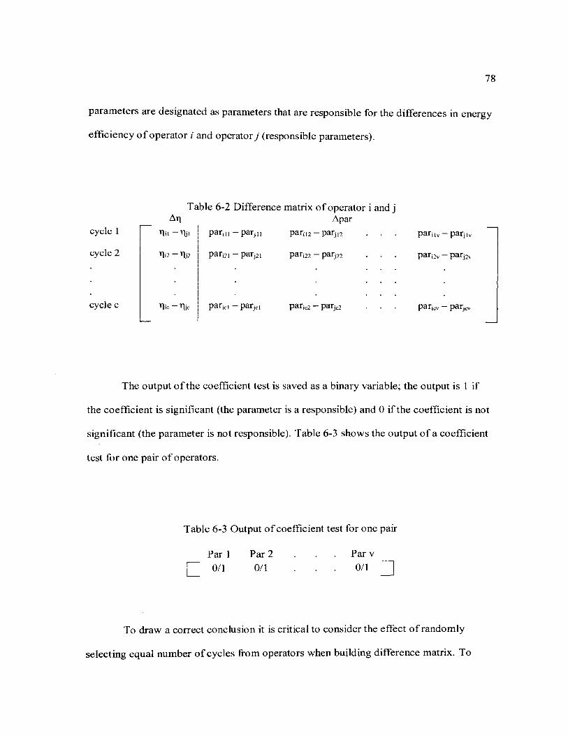
78
parameters are designated as parameters that are responsible for the differences in energy
efficiency of operator i and operator j (responsible parameters).
Table 6-2 Difference matrix of operator i and j ~11 ~par
cycle 1 llil -l]ji pari II - parj 11 paril2 - parj 12 parilv- parjlv
cycle 2 pari21 - parj2I pari22- parj22 pari2v - parj2v
cycle c llic -l]jc parici - parjci paric2 - parjc2
The output of the coefficient test is saved as a binary variable; the output is I if
the coefficient is significant (the parameter is a responsible) and 0 ifthe coefficient is not
significant (the parameter is not responsible). Table 6-3 shows the output of a coefficient
test for one pair of operators.
Table 6-3 Output of coefficient test for one pair
Par 1 c 011
Par 2
0/1
Parv
0/1 ~
To draw a correct conclusion it is critical to consider the effect of randomly
selecting equal number of cycles from operators when building difference matrix. To

79
reduce the effect of random sampling error, the process of selecting (ci-cj) cycles from
operator i for deletion and regression analysis is repeated k times. A parameter is a
responsible parameter, if in (1-a)% (at confidence level of a) ofruns it is recognized as a
responsible parameter (Table 6-4).
The algorithm of using linear regression of differences to fmd responsible
parameters can be found in Figure 6-2. In the main algorithm, the process of determining
responsible parameters using linear regression is repeated for each pair of operators
(Figure 6-1). From the result ofthe G) pair-wise comparisons the probability for a
parameter to be a responsible parameter (at confidence level of a) can be determined. The
case study is used to illustrate the suggested approach in the next section.
Table 6-4 Output of coefficient test and fmal conclusion of k runs (one pair)
Run 1 Run2
Runk
Final conclusion
Par 1
0/1 0/1
0/1
0/1 at
confidence level of a
Par 2 0/1 0/1
0/1
0/1 at
confidence level of a
Parv 0/1 0/1
0/1
0/1 at
confidence level of a

80
An example can help one to better understand the process of selecting equal
number of cycles and testing for being a responsible parameter. Let us say the purpose of
an experiment is to test whether the duration of warm up for a baseball player (a
parameter) is a contributor to differences in their batting average (energy efficiency). In
order to detect this relationship, k games of two players can be selected at random for
observation and to test the relationship. If in more than (1-a)% (at confidence level of a)
times the duration of warm up was a contributor to differences in the batting average
then it can be concluded that duration of warm up is a contributor, otherwise it is not a
contributor. The probability for duration of warm up to be a contributor can be calculated
by repeating this process for other pairs of players and counting the number of pairs in
which duration ofwarm up is recognized as a contributor. The case study is used to
illustrate the suggested approach in the next section.
6.4. CASE STUDY
To illustrate the suggested method the given data was used. The Accuweigh TM
monitoring system recorded 44 parameters for each cycle during the one month period of
data collection. Fourteen parameters were extracted from the data base as relevant
parameters for this work (see Section 4). MATLAB was used to perform Pearson
correlation analysis to detect the parameters correlated with dragline energy efficiency.

Select equal number of cycles
{at random)
Find the differences
Fit a linear regression model
Use the result of the significance
test of coefficients to determine
significant variables across 30
runs
Figure 6-2 Algorithm of using linear regression of differences to fmd significant parameters
81
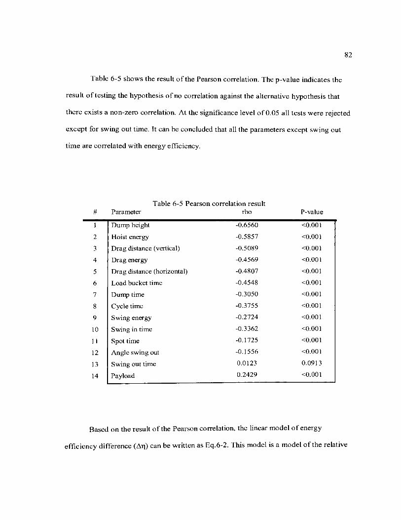
82
Table 6-5 shows the result of the Pearson correlation. The p-value indicates the
result oftesting the hypothesis of no correlation against the alternative hypothesis that
there exists a non-zero correlation. At the significance level of0.05 all tests were rejected
except for swing out time. It can be concluded that all the parameters except swing out
time are correlated with energy efficiency.
Table 6-5 Pearson correlation result # Parameter rho P-value
1 Dump height -0.6560 <0.001
2 Hoist energy -0.5857 <0.001
3 Drag distance (vertical) -0.5089 <0.001
4 Drag energy -0.4569 <0.001
5 Drag distance (horizontal) -0.4807 <0.001
6 Load bucket time -0.4548 <0.001
7 Dump time -0.3050 <0.001
8 Cycle time -0.3755 <0.001
9 Swing energy -0.2724 <0.001
10 Swing in time -0.3362 <0.001
11 Spot time -0.1725 <0.001
12 Angle swing out -0.1556 <0.001
13 Swing out time 0.0123 0.0913
14 Payload 0.2429 <0.001
Based on the result of the Pearson correlation, the linear model of energy
efficiency difference (~11) can be written as Eq.6-2. This model is a model ofthe relative

83
performance of the two operators. Drag, hoist, and swing energy consumption were not
included in the regression analysis, as energy efficiency is a representation of total energy
consumption and it is not necessary to include these parameters in the model.
~TJ=k0 +k1 x!VJh +k2 x!!JJDv +k3 x~Dh +k4 xl:!lb, +
k 5 x !!JJ, + k6 x ~c, + k7 x Mi, + k8 x M, + k9 x ~B" + k10 x M 6-2
Where Dh is dump height; DDv is drag distance (vertical); DDh is drag distance
(horizontal); lbt is load bucket time; Dt is dump time; C1 is cycle time; Si1 is swing in
time; St is Spot time; 9o is angle swing out; and P is payload.
Equal numbers of samples were selected at random for each pair of operators to
build the difference matrices (30 matrices per pair) ofthe pair. Linear regression was
used to fit Eq. 6-2 to the difference matrix data. The dependent variable is the difference
between energy efficiency and the differences between correlated parameters ( 1 0
parameters) were the independent variables. Testing for significance of coefficient was
carried out at 95% confidence level.
The process of linear regression analysis is repeated 30 times for each pair to
reduce the effect of random sampling. The result ofthe 30 runs for each pair can be found
in Table 6-6. Numbers in this table show the number of times in 30 runs that a parameter
in a pair-wise comparison is recognized as a parameter with significant coefficient or a
responsible parameter (i.e. the coefficient was non-zero at 95% confidence).

1
2
3
4
5
6
7
8
9
10
1
2
3
4
5
6
7
8
9
10
84
Table 6-6 Results ofthe 30 times run of regression analysis. Numbers indicate the number of times that a parameter is recognized as a parameter with significant
coefficient (responsible parameter)
Correlated parameters D,B D,E D,A D,C B,E
Dump height 30 30 30 30 30
Drag distance (vertical) 30 30 30 30 30
Drag distance (horizontal) 30 30 30 30 30
Load bucket time 4 30 26 30 0
Dump time 30 30 8 30 30
Cycle time 3 16 6 2 2
Swing in time 3 16 28 10 16
Spot time 30 30 30 30 30
Angle swing out 14 30 4 8 18
Payload 14 3 15 12 2
B,A B,C E,A E,C A,C
Dump height 30 30 30 30 30
Drag distance (vertical) 30 30 30 30 30
Drag distance (horizontal) 30 30 30 30 30
Load bucket time 8 20 5 22 30
Dump time 8 30 30 30 30
Cycle time 26 0 10 5 27
Swing in time 29 30 3 6 7
Spot time 30 30 21 30 30
Angle swing out 30 30 22 30 2
Payload 13 1 6 8 30

85
A parameter is recognized as a responsible parameter in each pair-wise
comparison if the number of having significant coefficient in 30 runs is more than 28
(confidence level of95%). Table 6-7 and Figure 6-3 show the results using the cut-off
value of28. The value of 1 is assigned to responsible parameters in each pair. The
probability column in Table 6-7and Figure 6-3 shows the estimated probability that a
parameter is a responsible parameter. Dump height, drag distance (vertical), and drag
distance (horizontal) have a 100% probability. It can be concluded that there is more than
95% chance of these parameters being responsible for differences in energy efficiency for
all 10 pairs of operators in the given dataset.
100% ... ~ 90% Q)
E ro ... ro 0. Q)
.0
80%
70%
60%
~ 50% 0 5r 40% Q) ... 30% ro ~ 20%
~ 10%
b -~ .0 ro
.0 0 ... a..
0%
Correlated Parameters
Figure 6-3 Estimated probability for correlated parameters to be responsible parameter

86
It can be concluded from Figure 6-3 and Table 6-7 that there is a high chance for
dump height, drag distance (v), drag distance (h), spot time, and dump time to be a
responsible parameter. On the other hand, for parameters such as cycle time, payload and,
swing in time the probability ofbeing a responsible parameter is relatively low.
Previous studies (Bogunovic & Kecojevic, 2011; Bogunovic, 2008; Erdem &
Diizgiin, 2005; Hettinger & Lumley, 1999; G. Lumley, 2005; Rai et al., 2000; Rai, 2004;
Torrance & Baldwin, 1990; Williams, 2005) have shown that payload, cycle time,
digging time and digging energy, fill factor, engagement and disengaeegement position
affect dragline productivity and energy consumption and, consequently, energy
efficiency. Also, Bogunovic and colleagues (Bogunovic & Kecojevic, 2011; Bogunovic,
2008) show that digging time (or loading bucket time in this work) was introduced as the
most important component of dragline cycle. The case study confirms these parameters
as important explanatory variables of drag line energy efficiency (Table 6-5). Dumping
height is shown to be highly correlated to energy efficiency (p = -0.6560, p < 0.001). This
has never been shown with experimental data, to the best of this author's knowledge. It
must be noted, however, that the fact that these parameters are correlated to energy
efficiency does not necessarily mean they are responsible for differences in operator
performance. Any of the parameters, that energy efficiency is sensitive to, can cause
differences in energy efficiency, if it varies significantly between operators.

D,B D,E
Dump height 1 1
Drag distance (vertical) 1 1
Drag distance (horizontal) I 1
Spot time I 1 Dump time I 1 Load bucket time 0 1 Angle swing out 0 1
Swing in time 0 0 Payload 0 0 Cycle time 0 0
Table 6-7 Final result based on assigning 0 and 1
D,A D,C B,E B,A B,C E,A E,C
1 1 1 1 1 1 1
1 1 1 1 1 1 1
I 1 1 1 1 1 1
I I 1 1 I 0 1 0 1 I 0 1 1 1 1 1 0 0 0 0 0 0 0 0 I I 0 1
1 0 0 0 I 0 0
0 0 0 0 0 0 0 0 0 0 0 0 0 0
A,C total
I 10
1 10
1 10
1 9 1 8 1 4 0 4
0 2 1 I
0 0
probability
100%
100%
100%
90% 80% 40% 40%
20% 10% 0%
00 -.l

88
In this case study, dumping height, vertical and horizontal drag distance, and
spotting and dump time are shown to be the primary parameters driving differences in
energy efficiency. Surprisingly, digging time, which has been identified by many
researchers as a key discriminator between operators (Bogunovic & Kecojevic, 2011;
Erdem & Diizgiin, 2005; Rai et al., 2000; Torrance & Baldwin, 1990; Williams, 2005),
was not found to be a significant factor between the five operators included in this study.
The result of this work shows that there is only a 40% probability that energy efficiency
of cycles from these operators is significantly different because of differences in digging
time. This probability is less than other cycle time components such as spotting and
dumping time. This shows that operator performance evaluation, which is based solely
on digging time or other parameters ofthe digging cycle (e.g. digging energy)
(Bogunovic, 2008; Komljenovic et al., 2010) can be misleading. On the other hand, drag
distance (vertical and horizontal) has a high chance ofbeing a responsible parameter.
This confirms the point that engagement and disengagement parameters are important
parameters and affect dragline performance (Hettinger & Lumley, 1999).
Payload and cycle time have been shown to affect productivity (Bogunovic, 2008;
Erdem & Diizgiin, 2005; G. Lumley, 2005; Williams, 2005). In the case study data set,
the correlation coefficients between energy efficiency and payload and cycle time are low
(0.2429 and -0.3755, respectively). However the results in Table 6-7 show that among the
five operators payload and cycle time have a low chance ofbeing a responsible parameter
and are not likely to cause differences in energy efficiency. It can be concluded that,
given a particular group of operators, not all parameters that are correlated with energy
efficiency are necessarily correlated to the difference of energy efficiency between

89
operators. That is, not all correlated parameters are the source of differences between
energy efficiency of operators. Hence, the methods proposed in this work are necessary
to fmd out which parameters are actually responsible for the differences in performance,
so that operator training can focus on these responsible parameters.
As discussed in Section 2, it is important to consider both productivity and energy
consumption in assessing dragline performance. Displaying energy efficiency, which
captures both production and energy consumption, in real-time on the screens in the cabin
can help operators to improve their performance. Identifying the parameters that affect
energy efficiency can be used as a guideline to improve the performance through operator
training and peer coaching.
6.5. SUMMARY
IdentifYing parameters that are responsible for the differences between energy
efficiency of operators can be used in operator training programs along with the crew
coaching method. The methodology proposed in this section is robust and can be used to
:fmd the probability for a parameter to be a responsible parameter. Correlation analysis
between parameters and energy efficiency can identify the correlated parameters. The
response mechanism, with respect to the missing data, is assumed to be missing at
random, in the worst case, and missing completely at random, in the best case. Hence,
complete case analysis can be used to handle the missing data issues associated with the
fact that pairs of operators will not, most likely, have equal number of cycles during the
observation period. Difference matrix of a pair of operators is built by subtracting
correlated parameters and energy efficiency of two operators in each cycle. Equal number

of cycles is selected at random, since having equal number of cycles in each pair is
required in order to create the difference matrix. Fitting linear model to the difference
matrix and testing the significance of coefficient can be used to identifY responsible
parameters (those parameters responsible for differences in energy efficiency).
90
The results achieved by applying the proposed method to the case study partially
confirm established results discussed in the literature review. Spotting and dumping time
were found to be more likely to be a responsible parameter than digging time (load
bucket time), contrary to some previous work. Engagement and disengagement position
of the bucket, as components of digging phase which have been found to be parameters
that affect productivity, were found to be very likely to cause differences in operator
energy efficiencies. No prior work (to the best of the author's knowledge) has discussed
the effect of dumping height on productivity or energy consumption. This work has
shown that dumping height is highly correlated to energy efficiency (p = -0.6560, p <
0.001) and also likely to be a responsible parameter (i.e. the source of differences in
operator energy efficiency).

91
7. CONCLUSIONS AND RECOMMENDATIONS
7.1. SUMMARY
Draglines are dominant machines and the most significant electricity consumers
in surface coal mines. With the growing price of energy and environmental concerns and
the high sensitivity of mines' profitability to dragline production, any improvement in
efficiency of dragline operations will be beneficial for mines. Training operators to
improve their performance can be a relatively cheap improvement and valid approach to
improve energy efficiency. The goals of this work were to: (i) test the hypothesis that
dragline operator's practices and skills significantly affect dragline energy efficiency; (ii)
develop a methodology to identify the critical parameters that explain the differences in
operator energy efficiency (responsible parameters).
To achieve the first objective of this work a two stage process was proposed. The
process is based on statistical tests to compare the mean of energy efficiency between
operators. The first stage involves evaluating the validity of assumptions underlying the
relevant statistical tests. This to ensure the analyst draws the right inferences about the
effect of operators on dragline energy efficiency given the data properties and to reduce
type I error. The second stage of the suggested process involved testing the equality of
means between energy efficiency of operators. Depending on the number ofthe operators
(two or more than two) two different processes for determining the appropriate test were
recommended.
A methodology was proposed to achieve the second goal of this work and to
identifY key parameters that lead to differences in operator energy efficiency (responsible
parameters). In this method, first, correlation analysis is used to detect the parameters in

92
the dataset that are correlated with energy efficiency. Difference matrices are then built
for each pair of operators. Linear regression is then used to determine the responsible
parameters. Data collected from a real mine was used to illustrate the presented methods
and tests. The data was recorded from a BE-1570w dragline with bucket capacity of85
yd3 during one month.
7.2. CONCLUSIONS
From the work it can be concluded that:
• Mean standard error of energy efficiency can be used to find the minimum
working hours required for an operator to be considered in the analysis in
order to have the same support from all operators. This approach is superior to
the previous approach suggested by Komlejenovi et al. (20 I 0) because it truly
goes to the heart ofthe problem (equal support for the different data sets).
Also, the approach suggested by Komlejenovi et al. (20I 0) fails (the lower
limit becomes negative) with highly variable working hours of operators
(Komljenovic et al., 20 I 0)
• Due to the high variability of dragline energy efficiency data (coefficient of
variation more than 25% in the case study) testing for normality can be
challenging. Considering the result ofboth numerical and graphical methods
can help to test the normality of the data or transformed data more precisely.

93
• Using t-test to compare the equality of means between more than two
operators can increase the chance of getting type 1 error. Therefore, pair-wise
t-tests are proposed in previous work increases the likelihood of type I error
as the number of operators in the study increases. However, AN OVA can
handle multiple (more than two) operators without increasing chance of
getting type 1 error.
• A valid method is proposed in this work facilitate accurate inferences on the
effect of operators on dragline energy efficiency in the presence of high
variability and data skewness. This method recommends the right statistical
test to draw the desired inferences based on observed data properties and
addresses the short comings, related to type 1 errors, of some of the previous
work. This novel method is illustrated successfully with real-life data.
• A novel and valid method is proposed in this work to evaluate the causes of
differences in energy efficiency, once operator effects on energy efficiency
have been established. The method is based on a linear model of the
differences in energy performance. The difference matrix (a matrix of the
differences in energy efficiency and explanatory variables) is calculated using
sound missing data theory to overcome the challenges of using real field data
in such analysis. This work is a novel attempt to combine statistical random
sampling, complete case analysis (missing data theory), and linear models of

relative energy efficiencies to establish causes of operator effects on energy
efficiency.
• The methods developed in this research were illustrated with a case study.
Several conclusions can be drawn based on this study of a single drag line.
Although these conclusions cannot be said to be widely applicable, they are
worth mentioning here:
94
o It was concluded from the result ofthe statistical tests, histograms, and Q
Q plots that energy efficiency of operators is not normality distributed and
the data has a right skewness. Log-transformation of data reduced the
skewness and it was concluded that log transformed data follows normal
distribution.
o The Levene's test with the null hypothesis of equality of variances on the
data was rejected. This result shows that using the ANOVA test could
result in wrong inferences since a key underlying assumption of ANOV A
tests is the equality of variances. This shows that in some cases the
previous approaches presented in the literature (Patnayak et al., 2007) can
lead to wrong inferences ifno systematic approach, like the methodology
developed in this research, is used to choose the right statistical test.

o The result ofthe Welch-ANOVA and Kruskal-Wallis tests on the data
proved that dragline energy efficiency is different between operators at
significant level of0.05.
95
o The parameters that are correlated with energy efficiency may not
necessarily be responsible for the differences between energy efficiency of
operators. Cycle time and payload were found to be correlated (p < 0.001)
with energy efficiency but not responsible for differences in operator
energy efficiencies.
o The results ofthe proposed method shows that there is a high chance for
dumping height, vertical and horizontal drag distances, spotting time, and
dumping time to be a responsible parameter. On the other hand, cycle
time, payload and, swing in time the probability of being a responsible
parameter is relatively low.
o For the first time (to the best of this author's knowledge) the effect of
dumping height on energy efficiency has been examined with field data
and found to be significant. The case study shows that it is highly
correlated to energy efficiency (p = -0.6560, p < 0.001) and also likely to
be a responsible parameter (100% ofthe time among the five operators
used in the case study).

96
o The case study shows that operator performance evaluation, based solely
on digging time or other parameters of the digging cycle alone (e.g.
digging energy) (Komljenovic et al., 201 0) can be misleading. Digging
time was not found to be a significant factor between the five operators
included in this study (only a 40% probability that energy efficiency of
cycles from the five operators are significantly different because of
differences in digging time). This probability is less than other cycle time
components such as spotting (90%) and dumping (80%) time.
7.3. RECOMMENDATIONS FOR FUTURE WORK
The following recommendations are made for future work:
• This work is limited because a linear model is used for the relative
energy efficiency of operators. In the future, the non-linear model
should be investigated to examine the effect of such a model on the
inferences. The proposed methodology will still be valid with a non
linear model, so long as a test for the significance of the coefficients of
the non-linear model can be formulated.
• A model for dragline energy efficiency can be built using additional
information on the characteristics of dragline motors such as gear
ratio, torque and etc. and more data on current and voltage signals.
This model can help to predict dragline energy efficiency in different

operating conditions. The model can be used to simulate different
operator practices and their effect on energy efficiency.
97
• Although care was taken during the field experiment to ensure similar
working conditions, parameters ofthe working conditions were not
recorded due to budget constraints that forced remote data collection.
Future experiments should endeavor to record working condition
parameters such as material properties, bench height, and weather
conditions to ensure operators are compared while working in the
same conditions.
• The proposed methods should be tested with data from other
draglines in other operations. This could include data collected from
other draglines with different bucket sizes, boom lengths, and drive
characteristics to observe the effect of data nuances that may not have
been observed in the test data.

APPENDIX A
LIST OF 44 PARAMETERS IN THE DATABASE

99
1. INTRODUCTION
APPENDIX A contains the list of 44 parameters in the database. The document
has been prepared as Microsoft Word 2010.

APPENDIXB
EXPERIMANTAL FIELD DATA

101
1. INTRODUCTION
APPENDIX B contains the experimental field data, collected from BE-1570w
dragline. The documents have been prepared as a Microsoft Excel2010.

102
BIBLIOGRAPHY
Acarog1u, 0., Ozdemir, L., & Asbury, B. (2008). A fuzzy logic model to predict specific energy requirement for TBM performance prediction. Tunnelling and Underground Space Technology, 23(5), 600--608. doi:l0.1016/j.tust.2007.11.003
Anderson, T. W. (1961). On the distribution of the two-sample Cramer-von Mises critetion. Annals of Mathematical Statisics.
Anderson, T. W., & Darling, D. A. (1952). Asymptotic theory of certain "goodness offit" criteria based on stochastic processes. Annals of mathematical statisitcs, 23(2).
Arch Coal Inc. (2012). Visitors Presentation in Coal Creek Mine.
Awuah-Offei, K., Frimpong, S., & Askari-Nasab, H. (2005). Dynamic simulation of cable shovel specific energy in oil sands excavation. Computer Applications in the Minerals Industry (CAM!).
Awuah-Offei, K., Osei, B., & Askari-Nasab, H. (2011). Modeling truck I shovel energy efficiency under uncertainty. Transactions of the society for mining, metallurgy and exploration, 330, 573-584.
Awuah-Offei, Kwame, Osei, B., & Askari-Nasab, H. (2012). Improving truck-shovel energy efficiency through discrete event modeling. SME Annual Meeting, (2010), 1-6.
Baafi, E. V, Mirabediny, H., & Whitchurch, K. (1995). A Simulation Model for Selecting Suitable Digging Method for a Dragline Operation. APCOM XXV, 9-14.
Biau, D. J. (2011). In brief: Standard deviation and standard error. Clinical orthopaedics and related research, 469(9), 2661-4. doi:10.1007/s11999-011-1908-9
Bogunovic, D. (2008). INTEGRATED DATA ENVIRONMENT FOR ANALYSIS AND CONTROL OF ENERGY CONSUMPTION (IDE-ACE) IN SURFACE COAL MINING. The Pennsylvania State University.
Bogunovic, D., & Kecojevic, V. (2011). Impact ofbucket fill factor on dragline production rate and energy consumption. Mining Engineering, 63(8), 48-53.
Bogunovic, D., Kecojevic, V., Lund, V., Heger, M., & Mongeon, P. (2009). ANALYSIS AND CONTROL OF ENERGY CONSUMPTION IN SURFACE COAL MINING. SME Annual Meeting, 1-7.

103
Bonskowski, R., Watson, W. D., & Freme, F. (2006). Coal production in the united states -an historical overview (pp. 1-19). Retrieved from http://www.eia.gov/cneaf/coal/page/coalyroduction_review.pdf
British Petroleum (BP). (2012). BP Statistical Review of World Energy June 2012. Retrieved from http://www.bp.com/statisticalreview
Bush, V., Killingsworth, T. G., & Ruffe1, E. P. (2002). Leveraging Your Energy Management Resources: Applications For The Mining Industry. SME Annual Meeting.
Cody, R. (2011). SAS Statistics by Example (p. 274). SAS Institute.
Cooley, C. M. (1955). Report on Akremite. Mining Engineering (pp. 25-28). AIME.
Demire1, N., & Frimpong, S. (2009). Drag1ine dynamic modelling for efficient excavation. International Journal of Mining, Reclamation and Environment, 2 3( 1 ), 4-20. doi:10.1080/17480930802091166
Dessureault, S. (2007). DATA MINING, MINING DATA: ENERGY CONSUMPTION MODELING Sean Dessureault. Proceedings of 33rd Symposium on Application of Computers and Operations Research in the Mineral Industry.
Dincer, I., & Rosen, M. A. (1999). Energy, environment and sustainable development. Applied Energy, 64, 1999.
Drezner, Z., Turel, 0., & Zerom, D. (2010). A Modified Kolmogorov-Smirnov Test for Normality. Communications in Statistics- Simulation and Computation, 39(4), 693-704. doi: 10.1080/03610911003615816
Drives & Controls Services. (2003). AccuWeigh production monitoring systems. Retrieved from http://www.drivesandcontrols.com/Assets/AccuWeigh Flyer.pdf
Dupriest, F., & Koederitz, W. (2005). Maximizing drill rates with real-time surveillance of mechanical specific energy. SPEIIADC Drilling Conference.
Erdem, B., & DUzgUn, H. ~- B. (2005). Dragline cycle time analysis. Journal of Scientific & Industrial Research, 64(January), 19-29.
Exxon Mobil. (2013). The outlook for energy: A view to 2040.
Gibbons, J.D., & Chakraborti, S. (2010). Nonparametric Statistical Inference (Fifth.).
Graham, J. W. (2009). Missing data analysis: making it work in the real world. Annual review of psychology, 60,549-76. doi:10.1146/annurev.psych.58.110405.085530

104
Harney, D. (2007). Measuring and controlling energy utilization. SME Annual Meeting.
Hawkes, P. J., Spathis, A. T., & Sengstock, G. W. (1995). Monitoring Equipment Productivity Improvements in Coal Mines. EXPLO Conference, (September).
Herberich, E., Sikorski, J., & Hathorn, T. (2010). A robust procedure for comparing multiple means under heteroscedasticity in unbalanced designs. PloS one, 5(3), e9788. doi:l 0.13 71/journal.pone.0009788
Hettinger, D., & Lumley, G. (1999). Using data analysis to improve dragline productivity. Coal Age.
Humphrey, J.D. (1990). The fundamentals of the dragline (pp. 1-28).
Iai, M., & Gertsch, L. (2013). EXCAVATION OF LUNAR REGOLITH WITH RAKES I RIPPERS FOR IMPROVED EXCAVATION EFFICIENCY. Journal of Aerospace Engineering, 26.
International Energy Agency (lEA). (2012). WORLD ENERGY OUTLOOK.
Johannes, B., Salnitski, V., SoU, H., Rauch, M., Goeters, K.-M., Maschke, P., Stelling, D., et al. (2007). Performance assessment in a flight simulator test-Validation of a space psychology methodology. Acta Astronautica, 60(4-7), 379-382. doi: 10.10 16/j.actaastro.2006.09 .006
Johnson, R. A., & Wichern, D. W. (2007). Applied Multivariate Statistical Analysis. Prentice Hall.
Karpuz, C., Ceylanoglu, A., & Pa~amehmetoglu, A. G. ( 1992). An investigation on the influence of depth of cut and blasting on shovel digging performance. International Journal ofSuiface Mining, Reclamation and Environment, 6(4), 161-167.
Kizil, M. (2010). improving Dragline Productivity using a Diggability index as an indicator. Society for Mining, Metallurgy & Exploration, Inc. (SME), 134-141.
Komljenovic, D., Bogunovic, D., & Kecojevic, V. (2010). Dragline operator performance indicator. International Journal of Mining, Reclamation and Environmet, 24(1), 34-43.
Krishnamoorthy, K., Lu, F., & Mathew, T. (2007). A parametric bootstrap approach for ANOV A with unequal variances: Fixed and random models. Computational Statistics & Data Analysis, 5I(l2), 5731-5742. doi: 10.1 016/j.csda.2006.09.039
Levene, H. (1960). Robust test for equality of variances. Stanford University Press, 278-
292.

Little, R. J. A. (1992). Regression With Missing X's: A Review. Journal~~ American Statistical Association, 87(420), 1227-1237.
105
Lumley, G. (2005). Reducing the Variability in Dragline Operator Performance Reducing the Variability in Dragline Operator Performance. Coal Operaotrs' Conference, 97-106.
Lumley, G. I. (2004). How to increase dragline productivity without spending too much money. Sixth Annual AJM Open Cut Coal Mining Conference.
Matuszak, R. A. (1982). How do you measure your dragline output? First Internationa SME-AIME Fall Meeting, (D).
McElduff, F., Cortina-Borja, M., Chan, S.-K., & Wade, A. (2010). When t-tests or Wilcoxon-Mann-Whitney tests won't do. Advances in physiology education, 34(3 ), 128-33. doi:10.1152/advan.00017.2010
Microsoft. (2008). SQL Server Management Studio.
Mielli, F. (2011). Three major mining challenges and their technological solutions. Minin, (september), 69-72.
Mielli, F., & Wallace, S. (2012). Energy plan for mining operations. Mining Engineering.
Morley, L.A., Trutt, F. C., & Buchan, G. M. (1982). ELECTRICAL· SHOCK PREVENTION VOLUME III- FAULT PROTECTION FOR MOTION· DRIVE EQUIPMENT.
Morrison, R., & Scott, A. (2002). Maximising the Value of" A Wealth oflnformation ". Value Tracking Symposium, (October), 7-8.
Muro, T., Tsuchiya, K., & Kohno, K. (2002). Experimental considerations for steady state edge excavation under a constant cutting depth for a mortar specimen using a disk cutter bit. Journal ofTerramechanics, 39(3), 143-159. doi: 10.1 016/S0022-4898(02)00021-6
National Mining Association (NMA). (2012). The Economic Contributions ofU.S. Mining in 2010, (September). Retrieved from http://www.nma.org/pdfi'economic_contributions.pdf
Norman, S. (2011). VARIABILITY REDUCTION IN DRAGLINE OPERATOR PERFORMANCE. SME Annual Meeting, 1-2.
Orner, A. M. (2008). Energy, environment and sustainable development. Renewable and Sustainable Energy Reviews, I 2(9), 2265-2300. doi: 10.1016/j.rser.2007.05.001

Orica Mining Services. (2010). Energy and Emissions: Initiatives towards a more sustainable future. Retrieved from https://www .oricaminingservices. com/up loads/Collateral/Coal/Resource Value Maximisation/Minimise Coal Loss/Products and Services/6. I. Sustainabi lity Brochure.pdf
106
Park, H. M. (2008). Analysis and Normality Test Using SAS, Stata, and SPSS. Indiana University, University Information Technology Services Univariate.
Patnayak, S., Tannant, D. D., Parsons, I., Del Valle, V., & Wong, J. (2007). Operator and dipper tooth influence on electric shovel performance during oil sands mining. International Journal of Mining, Reclamation and Environment, 1-26. doi: 10.1080/17480930701482961
Pippenger, J. G. (1995). Competing with the big boys: Productivity and innovation at the Freedom lignite mine, 3-6.
PRB Coal Properties. (2013). Retrieved from http://www.cbassd.com/Applications/knowledgeBase/PRBcoal!PRBcoalProperty.htm
Rai, P. (2004). Performance assessment of draglines in opencast mines. Indian Journal !f Engineering & Material Sciences, JJ(December), 493-498.
Rai, P., Ratnesh, T., & Nath, R. (2000). Cycle time and idle time analysis of draglines for increased productivity--A case study. Indian Journal of Engineering & Material Sciences, 7, 77-81.
Ristic, L. B., & Jefteni, B. I. (2012). Implementation of Fuzzy Control to Improve Energy Efficiency ofVariable Speed Bulk Material Transportation, 59(7), 2959-2969.
Rodgers, J. L., & Nicewander, A. W. (1988). Thirteen Ways to Look at the Correlation Coefficient. The American Statistician, 42(1), 59-66.
Rowlands, C., & Just, G. D. (1992). Performance Characteristics ofDragline Buckets. Third Large Open Pit Conference, (September), 89-92.
SAS Institute inc. (2011). SAS® 9.3.
Schafer, J. L., & Graham, J. W. (2002). Missing data: Our view of the state of the art. Psychological Methods, 7(2), 147-177. doi: 1 0.1037//1082-989X.7.2.147
Schlotzhauer, S. D. (2009). Elementary Statistics Using SAS®. SAS Institute.
Schultz, B. B. (1983). On Levene's test and other statistics ofvariation. Evolutionary Theory.

107
Shapiro, S S, Wilk, M. B., & Chen, H. J. (1968). A Comparative Study ofYarious Tests for Normality, 63(324), 1343-1372.
Shapiro, S. S., & Wilk, M. B. (1965). An analysis of variance test for normality (complete samples). Biometrika Trust, 52(3), 591-611.
Sheskin, D. J. (2004). Handbook ofParametric and Nonparametric Statistical Procedures. Chapman & Hall. Retrieved from http:/ /books.google.com/books?id=bmwhcJqqO 1 cC&pg=P A59#v=onepage&q&f=fa lse
Steele, R., & Sterling, D. (2011). Identifying opportunities to reduce the consumption of energy across mining and mineral processing plants. SME Annual Meeting.
Stephens, M.A. (1974). EDF Statistics for Goodness ofFit and Some Comparisons. Theory and Methods Section, 69(347), 730-737.
Stricker, G. D., Flores, R. M., Trippi, M. H., Ellis, M. S., Olson, C. M., Sullivan, J. E., & Takahashi, K. I. (2007). Coal Quality and Major, Minor, and Trace Elements in the Powder River, Green River, and Williston Basins, Wyoming and North Dakota. Retrieved from http:l/pubs.usgs.gov/o£'2007/1116/
Teale, R. (1965). The concept of specific energy in rock drilling. International Journal of Rock Mechanics and Mining Sciences & Geomechanics, 2, 57-73.
The MathWorks Inc. (2011). MATLAB (R2011a).
Torrance, A., & Baldwin, G. (1990). Blast Performance Assessment using a Dragline Monitor. Third International Symposium on Rock Fragmentation by Blasting, 219-224.
Truxillo, C. (2002). Maximum Likelihood Parameter Estimation with Incomplete Data. SUGI 30, 1-19.
U.S. Department ofEnergy(DOE). (2007). Mining Industry Energy Bandwidth Study. U.S. Department of Energy.
U.S. Energy Information Administration (EIA). (2011a). International Energy Statistics. Retrieved from http://www .eia.gov/cfapps/ipdbproject/IEDindex3 .cfm ?tid= 1 &pid= 1 &aid=2
U.S. Energy Information Administration (EIA). (2011b). Annual Coal Report (Vol. 2010).
U.S. Energy Information Administration (EIA). (2011c). Annual Energy Review 2011.

108
U.S. Energy Information Administration (EIA). (2012). What is the average heat (Btu) content of US. coal? Retrieved from http://www.eia.gov/tools/faqs/faq.cfin?id=72&t=2
U.S. Energy Information Administration (EIA). (2013). Voluntary Reporting of Greenhouse Gases Program. Retrieved from http://www.eia.gov/oia£11605/
U.S. Energy Infromation Administration. (2012). Electric Power Monthly. Retrieved from http://www.eia.gov/electricity/monthly/
United States Environmental Protection Agency (EPA). (2004). Attachment 5 The Powder River Basin (pp. 1-20).
USGS. (2008). Assessment of Coal Geology, Resources, and Reserves in the Gillette Coalfield, Powder River Basin , Wyoming Assessment of Coal Geology , Resources , and Reserves in the Gillette Coalfield, Powder River Basin, Wyoming.
Van Valen, L. (1978). The statistics ofvariation. Evolutionary Theory, 33-43.
Vasilescu, I., Detweiler, C., Doniec, M., Gurdan, D., Sosnowski, S., Stumpf, J., & Rus, D. (2010). AMOUR V: A Hovering Energy Efficient Underwater Robot Capable of Dynamic Payloads. International Journal Of Robotics Research, 547-570.
Vista. (2013). A More Intelligent Approach to Haul Truck Operator Training. Retrieved from http://www.vista-training.com/assets/pdflbrochures/vista-trucklogicbrochure. pdf
Vynne, J. F .. (2008). Innovative Dragline Monitoring Systems and Technologies. CIM Conference.
Welch, B. L. (1947). The Generalization of'Student's' Problem when Several Different Population Variances are Involved. Biometrika Trust, 34(1), 28-35.
Williams, G. (2005). Achievements through the dragline improvement group (DIG) in Anglo coal. Institute of quarrying southern Africa.
World Energy Council. (2010). 2010 Survey of Energy Resources (p. 618).
Wyoming State Geological Survey. (2010). Wyoming State Geological Survey. Retrieved January 19, 2013, from http://www.wsgs.uwyo.edu/datalgis/PRB-Info.aspx
Zhou, X. H., Gao, S., & Hui, S. L. (1997). Methods for comparing the means oftwo independent log-normal samples. Biometrics, 53(3), 1129-35. Retrieved from http://www .ncbi. nlm.nih.gov/pubmed/9290231

Zhu, Y. Q., & Yin, Z. D. (2008). A new evaluation system for energy saving based on energy efficiency and loss ratio. International Conference on Sustainable Energy Technologies (ICSET), Singapore: IEEE, 121-124.
109

110
VITA
Maryam Abdioskouei was born in Tehran, Iran, on 22 March 1988. After
completing her degree at Farzanegan high school under supervision ofNational
Organization for Development of Exceptional Talents (NODET) in 2006, she went on to
Amirkabir University of Technology (Formerly called Tehran Polytechnic),where she
studied mining engineering and received her Bachelor of Science in April 2011. In 2011,
she entered graduate college at Missouri University of Science and Technology at Rolla,
Missouri where she is studying Mining Engineering. She hopes to receive her Master's
degree in August 2013. Maryam has been a member ofthe Society of Mining and
Metallurgical Engineers (SME) since 2011.