Methods for performance evaluation and optimization on modern HPC systems

Felix Wolf 08-06-2011

Objectives

•  Learn about basic performance measurement and analysis methods and techniques for HPC applications

•  Get to know Scalasca, a scalable and portable performance analysis tool

Performance tuning: an old problem

“The most constant difficulty in contriving the engine has arisen from the desire to reduce the time in which the calculations were executed to the shortest which is possible.”

Charles Babbage 1791 - 1871

Outline

•  Principles of parallel performance •  Performance analysis techniques •  Practical performance analysis using Scalasca

Mo#va#on  

Source:  Wikipedia  

Why parallelism at all? Moore's Law is still in charge…

Mo#va#on  Free lunch is over…

Parallelism

•  System/application level –  Server throughput can be improved by spreading workload

across multiple processors or disks –  Ability to add memory, processors, and disks is called scalability

•  Individual processor –  Pipelining –  Depends on the fact that many instructions do not depend on the

results of their immediate predecessors

•  Detailed digital design –  Set-associative caches use multiple banks of memory –  Carry-lookahead in modern ALUs

Amdahl’s Law for parallelism

•  Assumption – program can be parallelized on p processors except for a sequential fraction f with

•  Speedup limited by sequential fraction

€

0 ≤ f ≤1

€

Speedup(p) =1

f +1− fp

<1f

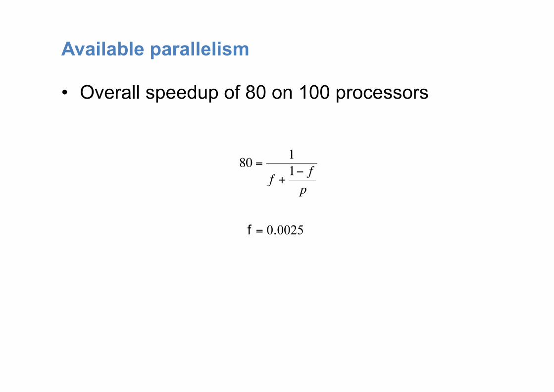
Available parallelism

•  Overall speedup of 80 on 100 processors

€

80 =1

f +1− fp

Law of Gustafson

•  Amdahl’s Law ignores increasing problem size –  Parallelism often applied to calculate bigger problems instead of

calculating a given problem faster

•  Fraction of sequential part may be function of problem size

•  Assumption –  Sequential part has constant runtime –  Parallel part has runtime

•  Speedup

If    parallel  part  can  be  perfectly  parallelized  

Parallel efficiency

•  Metric for cost of parallelization (e.g., communication) •  Without super-linear speedup

•  Super-linear speedup possible –  Critical data structures may fit into the aggregate cache

Scalability

•  Weak scaling –  Ability to solve a larger input problem by using more resources

(here: processors) –  Example: larger domain, more particles, higher resolution

•  Strong scaling –  Ability to solve the same input problem faster as more resources

are used –  Usually more challenging –  Limited by Amdahl’s Law and communication demand

Serial vs. parallel performance

•  Serial programs –  Cache behavior and ILP

•  Parallel programs –  Amount of parallelism –  Granularity of parallel tasks –  Frequency and nature of inter-task communication –  Frequency and nature of synchronization

•  Number of tasks that synchronize much higher → contention

Goals of performance analysis

•  Compare alternatives –  Which configurations are best under which conditions?

•  Determine the impact of a feature –  Before-and-after comparison

•  System tuning –  Find parameters that produce best overall performance

•  Identify relative performance –  Which program / algorithm is faster?

•  Performance debugging –  Search for bottlenecks

•  Set expectations –  Provide information for users

Analysis techniques (1)

•  Analytical modeling –  Mathematical description of the system –  Quick change of parameters –  Often requires restrictive assumptions rarely met in practice

•  Low accuracy –  Rapid solution –  Key insights

•  Validation of simulations / measurements

•  Example –  Memory delay

–  Parameters obtained from manufacturer or measurement

Analysis techniques (2)

•  Simulation –  Program written to model important features of the system being

analyzed –  Can be easily modified to study the impact of changes –  Cost

•  Writing the program •  Running the program

–  Impossible to model every small detail •  Simulation refers to “ideal” system •  Sometimes low accuracy

•  Example –  Cache simulator –  Parameters: size, block size, associativity, relative cache and

memory delays

Analysis techniques (3)

•  Measurement –  No simplifying assumptions –  Highest credibility –  Information only on specific system being measured –  Harder to change system parameters in a real system –  Difficult and time consuming –  Need for software tools

•  Should be used in conjunction with modeling –  Can aid the development of performance models –  Performance models set expectations against which

measurements can be compared

Metrics of performance

•  What can be measured? –  A count of how many times an event occurs

•  E.g., Number of input / output requests –  The duration of some time interval

•  E.g., duration of these requests –  The size of some parameter

•  Number of bytes transmitted or stored

•  Derived metrics –  E.g., rates / throughput –  Needed for normalization

Primary performance metrics

•  Execution time, response time –  Time between start and completion of a program or event –  Only consistent and reliable measure of performance –  Wall-clock time vs. CPU time

•  Throughput –  Total amount of work done in a given time

•  Performance =

•  Basic principle: reproducibility •  Problem: execution time is slightly non-deterministic

–  Use mean or minimum of several runs

1  

Execu:on  :me  

Alternative performance metrics

•  Clock rate •  Instructions executed

per second •  FLOPS

–  Floating-point operations per second

•  Benchmarks –  Standard test program(s) –  Standardized methodology –  E.g., SPEC, Linpack

•  QUIPS / HINT [Gustafson and Snell, 95] –  Quality improvements per second –  Quality of solution instead of effort to reach it

“Math” operations? HW operations?

HW instructions? Single or double

precision?

Comparison of analysis techniques

Analytical modeling

Simulation Measurement

Flexibility High High Low

Cost Low Medium High

Credibility Low Medium High

Accuracy Low Medium High

Peak performance

•  Peak performance is the performance a computer is guaranteed not to exceed

Source:  Hennessy,  Pa@erson:  Computer  Architecture,  4th  edi:on,  Morgan  Kaufmann  

64  processors  

Performance tuning cycle

Instrumenta:on  

Measurement  

Analysis  

Presenta:on  

Op:miza:on  

Performance measurement cycle (2)

•  Instrumentation –  Insertion of extra code (probes) into application

•  Measurement –  Collection of data relevant to performance analysis

•  Analysis –  Calculation of metrics –  Identification of performance bottlenecks

•  Presentation –  Transformation of the results into a representation that can be

easily understood by a human user

•  Optimization –  Elimination of bottlenecks

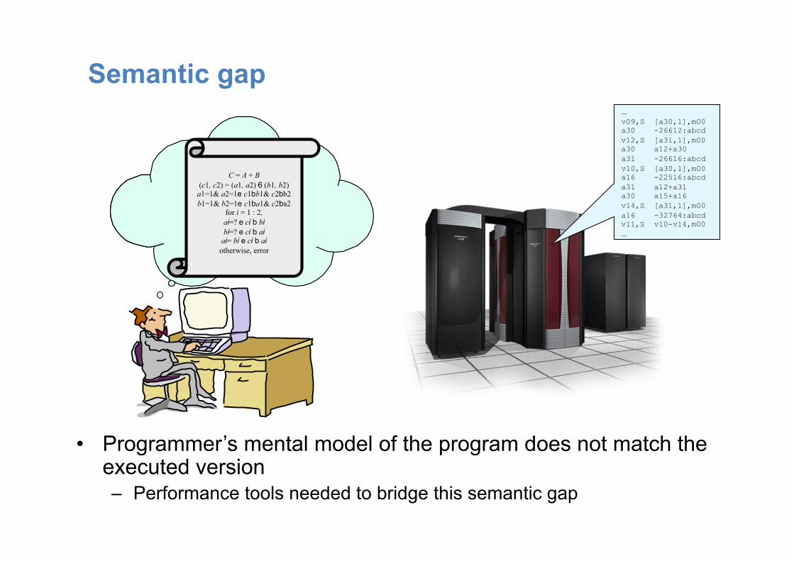
Semantic gap

•  Programmer’s mental model of the program does not match the executed version –  Performance tools needed to bridge this semantic gap

C = A + B (c1, c2) = (a1, a2) 6 (b1, b2)

a1=1& a2=1e c1bb1& c2bb2 b1=1& b2=1e c1ba1& c2ba2

for i = 1 : 2, ai=? e ci b bi bi=? e ci b ai

ai= bi e ci b ai otherwise, error

... v09,S [a30,1],m00 a30 -26612:abcd v12,S [a31,1],m00 a30 a12+a30 a31 -26616:abcd v10,S [a30,1],m00 a16 -22516:abcd a31 a12+a31 a30 a15+a16 v14,S [a31,1],m00 a16 -32764:abcd v11,S v10-v14,m00 ...

Semantic performance mapping

•  Instrumentation levels –  Source code –  Library –  Runtime system –  Object code –  Operating system –  Runtime image –  Virtual machine

•  Problem –  Every level provides different information –  Often instrumentation on multiple levels required

•  Challenge –  Mapping performance data onto application-level abstraction

Instrumentation techniques

•  Static instrumentation –  Program is instrumented prior to execution

•  Dynamic instrumentation –  Program is instrumented at runtime

•  Code is inserted –  Manually –  Automatically

•  By preprocessor •  By compiler •  By linking against preinstrumented (interposition) library •  By binary-rewrite / dynamic instrumentation tool

Measurement

Typical performance data include •  Counts •  Durations

•  Communication cost •  Synchronization cost •  IO accesses •  System calls •  Hardware events

inclusive  dura:on  

exclusive  dura:on  

int foo() { int a;

a = a + 1;

bar();

a = a + 1; }

Critical issues

•  Accuracy –  Perturbation

•  Measurement alters program behavior •  E.g., memory access pattern

–  Intrusion overhead •  Measurement itself needs time and thus lowers performance

–  Accuracy of timers, counters

•  Granularity –  How many measurements

•  Pitfall: short but frequently executed functions –  How much information / work during each measurement

•  Tradeoff –  Accuracy ⇔ expressiveness of data

Single-node performance

•  Huge gap between CPU and memory speed

•  Internal operation of a microprocessor potentially complex –  Pipelining –  Out-of-order instruction issuing –  Branch prediction –  Non-blocking caches

Source:  Hennessy,  Pa@erson:  Computer  Architecture,  4th  edi:on,  Morgan  Kaufmann  

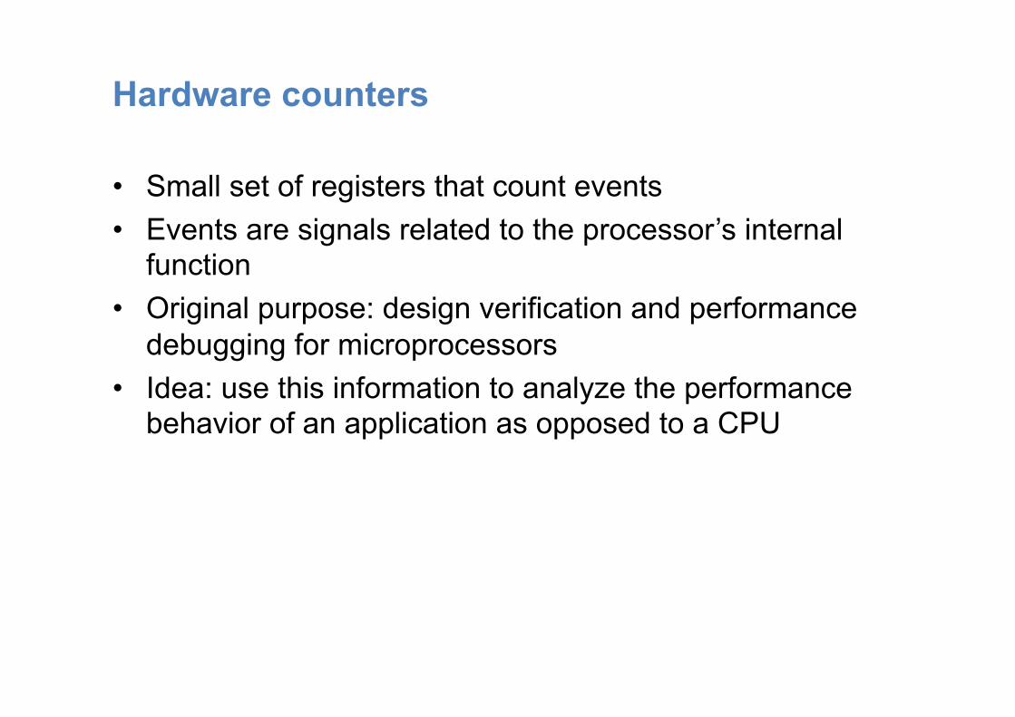
Hardware counters

•  Small set of registers that count events •  Events are signals related to the processor’s internal

function •  Original purpose: design verification and performance

debugging for microprocessors •  Idea: use this information to analyze the performance

behavior of an application as opposed to a CPU

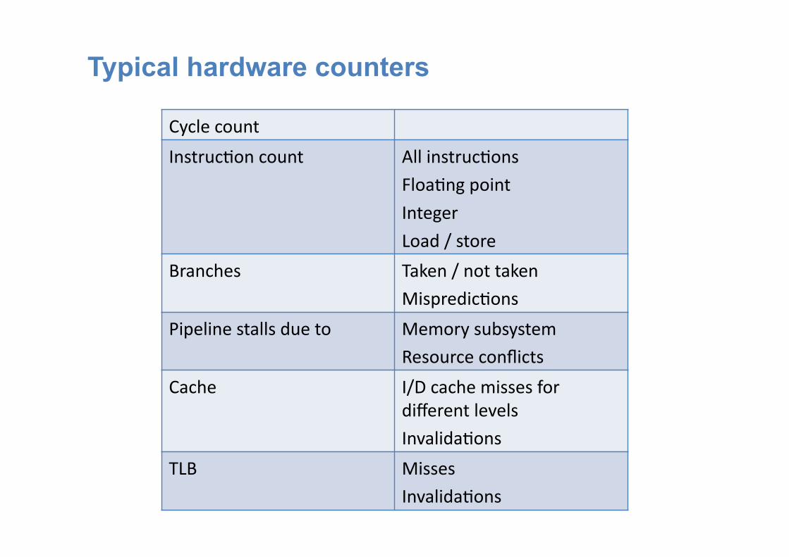
Typical hardware counters

Cycle  count Instruc:on  count All  instruc:ons  

Floa:ng  point  

Integer  

Load  /  store Branches Taken  /  not  taken  

Mispredic:ons Pipeline  stalls  due  to Memory  subsystem  

Resource  conflicts Cache I/D  cache  misses  for  

different  levels  

Invalida:ons TLB Misses  

Invalida:ons

Profiling

•  Mapping of aggregated information –  Time –  Counts

•  Calls •  Hardware counters

•  Onto program and system entities –  Functions, loops, call paths –  Processes, threads

•  Methods to create a profile –  PC sampling (statistical approach) –  Interval timer / direct measurement (deterministic approach)

Profiling (2)

•  Sampling –  Statistical measurement technique

•  Based on the assumption that a subset of a population being examined is representative for the whole population

•  Requires long-running programs –  Periodic operating system signal interrupts the running program –  Interrupt service routine examines return-address stack to find

address of instruction being executed when interrupt occurred –  Using symbol-table information this address is mapped onto

specific subroutine

•  Interval timing –  Time measurement at beginning and end of a code region –  Requires high-resolution / low-overhead clock

Call-path profiling

•  Behavior of a function may depend on caller (i.e., parameters)

•  Flat function profile often not sufficient

•  How to determine call path at runtime? –  Runtime stack walk –  Maintain shadow stack

•  Requires tracking of function calls

main() { A( ); B( ); }

A( ) B( ) { { X(); Y(); Y(); } }

main  

A  

B  

X  

Y  

Y  

Event tracing

Section on display

•  Typical events –  Entering and leaving a function –  Sending and receiving a message

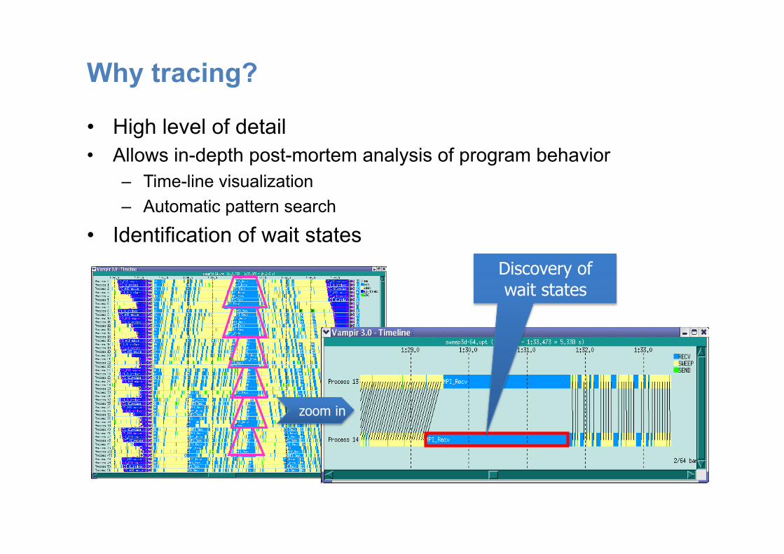
Why tracing?

•  High level of detail •  Allows in-depth post-mortem analysis of program behavior

–  Time-line visualization –  Automatic pattern search

•  Identification of wait states Discovery of wait states

zoom in

Obstacle: trace size

•  Problem: width and length of event trace

Number of processes

t

Wid

th

Execution time

t

t

long

short

Event frequency

t

t

high

low

Tracing vs. profiling

•  Advantages of tracing –  Event traces preserve the temporal and spatial relationships

among individual events –  Allows reconstruction of dynamic behavior of application

on any required abstraction level –  Most general measurement technique

•  Profile data can be constructed from event traces

•  Disadvantages –  Traces can become very large –  Writing events to a file at runtime can cause perturbation –  Writing tracing software is complicated

•  Event buffering, clock synchronization, …

•  Scalable performance-analysis toolset for parallel codes –  Focus on communication & synchronization

•  Integrated performance analysis process –  Performance overview on call-path level via call-path profiling –  In-depth study of application behavior via event tracing

•  Supported programming models –  MPI-1, MPI-2 one-sided communication –  OpenMP (basic features)

•  Available for all major HPC platforms

Joint project of

The team

www.scalasca.org

Installations and users •  Companies

–  Bull (France) –  Dassault Aviation (France) –  Efield Solutions (Sweden) –  GNS (Germany) –  INTES (Germany) –  MAGMA (Germany) –  RECOM (Germany) –  SciLab (France) –  Shell (Netherlands) –  Sun Microsystems (USA, Singapore, India) –  Qontix (UK)

•  Research/supercomputing centers –  ANL (USA)BSC (Spain) –  CASPUR (Italy) –  CEA (France) –  CERFACS (France) –  CINECA (Italy) –  CSC (Finland) –  CSCS (Switzerland) –  DLR (Germany) –  DKRZ (Germany) –  EPCC (UK) –  FZJ (Germany) –  HLRN (Germany) –  HLRS (Germany) –  ICHEC (Ireland) –  IDRIS (France) –  KIT (Germany) –  LLNL (USA)

•  Research/supercomputing centers (cont.) –  LRZ (Germany) –  MCH (Switzerland) –  NCAR (USA) –  NCSA (USA) –  ORNL (USA) –  PIK (Germany) –  PSC (USA) –  RZG (Germany) –  SARA (Netherlands) –  SAITC (Bulgaria) –  TACC (USA)

•  Universities –  Lund University (Sweden) –  MSU (Russia) –  RPI (USA) –  RWTH (Germany) –  TUD (Germany) –  UOregon (USA) –  UTK (USA)

•  DoD/MoD computing centers –  AFRL DSRC (USA) –  ARL DSRC (USA) –  ARSC DSRC (USA) –  AWE (UK) –  ERDC DSRC (USA) –  Navy DSRC (USA) –  MHPCC DSRC (USA) –  SSC-Pacific (USA) –  MetOffice (UK)

Which  problem?  Where  in  the  program?  

Which  process?  

Parallel  wait-­‐state  search  

Summary  report  

Wait-­‐state  report  

Instr.  target  applica:on    

Measurement  library  

HWC   Local  event  traces  

Op:mized  measurement  configura:on  

Instrumenter  compiler  /  linker  

Instrumented  executable  

Source  modules  

Repo

rt    

manipula:

on  

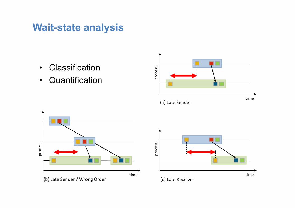
Wait-state analysis

•  Classification •  Quantification

:me  

process  

(a)  Late  Sender  

:me  

process  

(c)  Late  Receiver  :me  

process  

(b)  Late  Sender  /  Wrong  Order  

XNS CFD simulation application

•  Computational fluid dynamics code –  Developed by Chair for Computational Analysis of Technical

Systems, RWTH Aachen University –  Finite-element method on unstructured 3D meshes –  Parallel implementation based on message passing –  >40,000 lines of Fortran & C –  DeBakey blood pump test case

•  Scalability of original version limited <1024 CPUs

Par::oned  finite-­‐element  mesh  

Call-path profile: Computation

Execu:on  :me  excl.  MPI  comm  

Just  30%  of  simula:on  

Widely  spread  in  code  

Widely  spread  in  code  

Widely  spread  in  code  

Call-path profile: P2P messaging

P2P  comm  66%  of  

simula:on   Primarily  in  sca@er  &  gather  

Primarily  in  sca@er  &  gather  

MPI  point-­‐  to-­‐point    communic-­‐  a:on  :me  

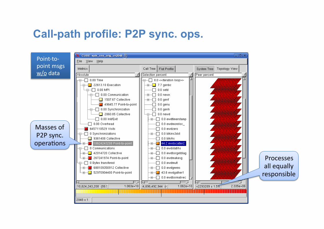
Call-path profile: P2P sync. ops.

Masses  of  P2P  sync.  opera:ons  

Processes  all  equally  responsible  

Point-­‐to-­‐  point  msgs  w/o  data  

Trace analysis: Late sender

Half  of  the  send  :me      is  wai:ng  

Significant  process  imbalance  

Wait  :me  of  receivers  blocked  for  late  sender  

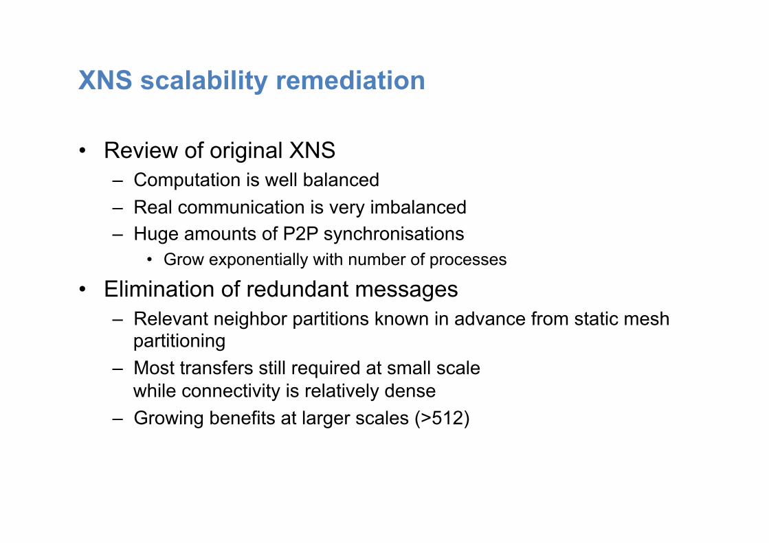
XNS scalability remediation

•  Review of original XNS –  Computation is well balanced –  Real communication is very imbalanced –  Huge amounts of P2P synchronisations

•  Grow exponentially with number of processes

•  Elimination of redundant messages –  Relevant neighbor partitions known in advance from static mesh

partitioning –  Most transfers still required at small scale

while connectivity is relatively dense –  Growing benefits at larger scales (>512)

After removal of redundant messages

Original  performance  peaked  at    132  ts/hr  

Revised  version  con:nues  to  scale  

XNS wait-state analysis of tuned version

MAGMAfill by MAGMASOFT® GmbH

•  Simulates mold-filling in casting processes

•  Scalasca used –  To identify communication

bottleneck –  To compare alternatives using

performance algebra utility

•  23% overall runtime improvement

INDEED by GNS® mbh

•  Finite-element code for the simulation of material-forming processes

–  Focus on creation of element-stiffness matrix

•  Tool workflow –  Scalasca identified serialization in critical

section as bottleneck –  In-depth analysis using Vampir

•  Speedup of 30-40% after optimization

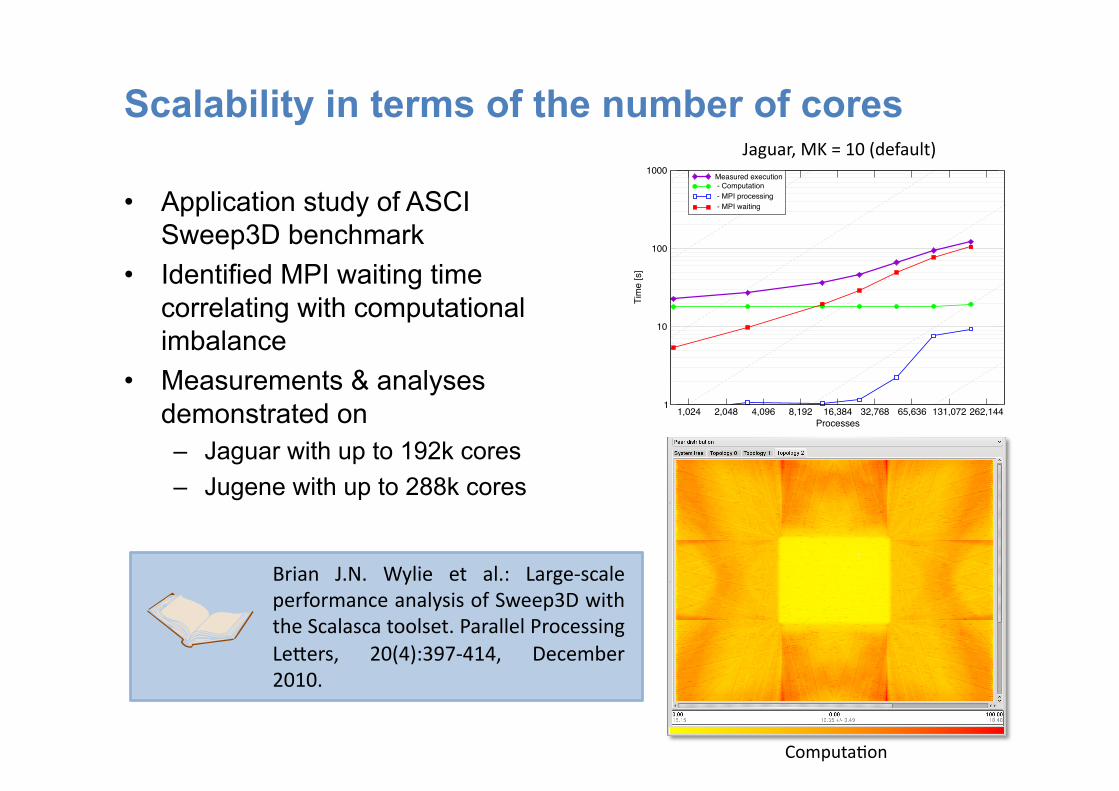
Scalability in terms of the number of cores

•  Application study of ASCI Sweep3D benchmark

•  Identified MPI waiting time correlating with computational imbalance

•  Measurements & analyses demonstrated on –  Jaguar with up to 192k cores –  Jugene with up to 288k cores

1,024 2,048 4,096 8,192 16,384 32,768 65,636 131,072 262,144Processes

1

10

100

1000

Tim

e [s

]

Measured execution - Computation - MPI processing - MPI waiting

Brian   J.N.   Wylie   et   al.:   Large-­‐scale  performance  analysis  of  Sweep3D  with  the  Scalasca  toolset.  Parallel  Processing  Le@ers,   20(4):397-­‐414,   December  2010.  

Jaguar,  MK  =  10  (default)  

Computa:on  

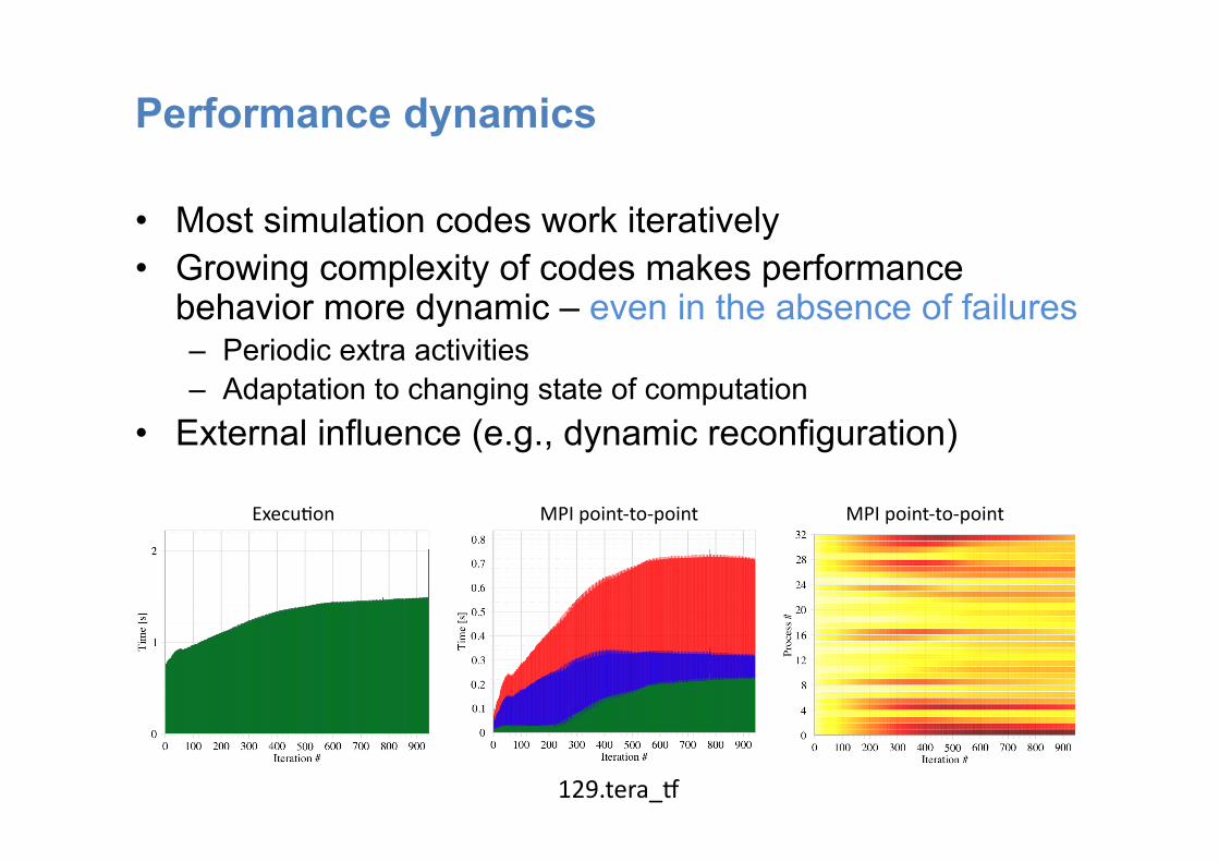
Performance dynamics

•  Most simulation codes work iteratively •  Growing complexity of codes makes performance

behavior more dynamic – even in the absence of failures –  Periodic extra activities –  Adaptation to changing state of computation

•  External influence (e.g., dynamic reconfiguration)

129.tera_i  

MPI  point-­‐to-­‐point   MPI  point-­‐to-­‐point  Execu:on  

P2P communication in SPEC MPI 2007 suite

107.leslie3d   113.GemsFDTD   115.fds4   121.pop2  

126.leslie3d   128.GAPgeofem   129.tera_i  127.wrf2  

130.socorro   132.zeusmp2   137.lu  

Scalasca’s approach to performance dynamics

•  Capture overview of performance dynamics via time-series profiling –  Time and count-based metrics

•  Identify pivotal iterations –  If reproducible

•  In-depth analysis of these iterations via tracing –  Analysis of wait-state formation

including root cause analysis –  Tracing restricted to iterations of interest

New  

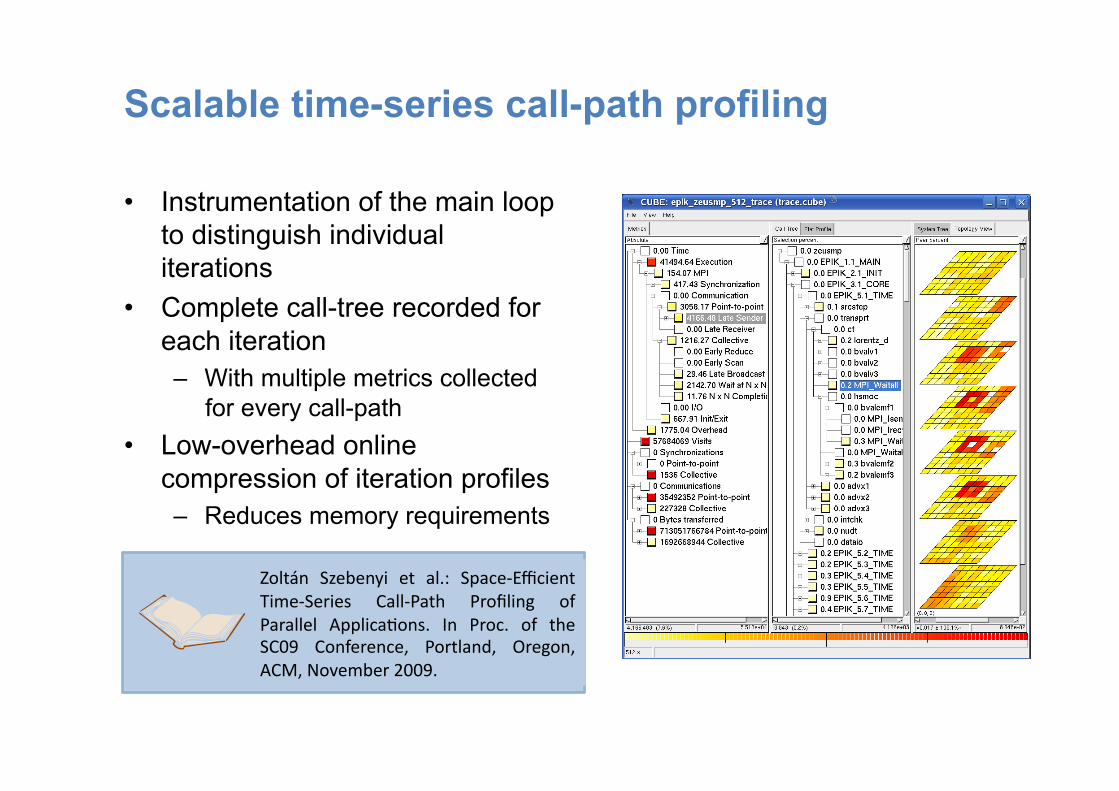
Scalable time-series call-path profiling

•  Instrumentation of the main loop to distinguish individual iterations

•  Complete call-tree recorded for each iteration –  With multiple metrics collected

for every call-path •  Low-overhead online

compression of iteration profiles –  Reduces memory requirements

Zoltán   Szebenyi   et   al.:   Space-­‐Efficient  Time-­‐Series   Call-­‐Path   Profiling   of  Parallel   Applica:ons.   In   Proc.   of   the  SC09   Conference,   Portland,   Oregon,  ACM,  November  2009.  

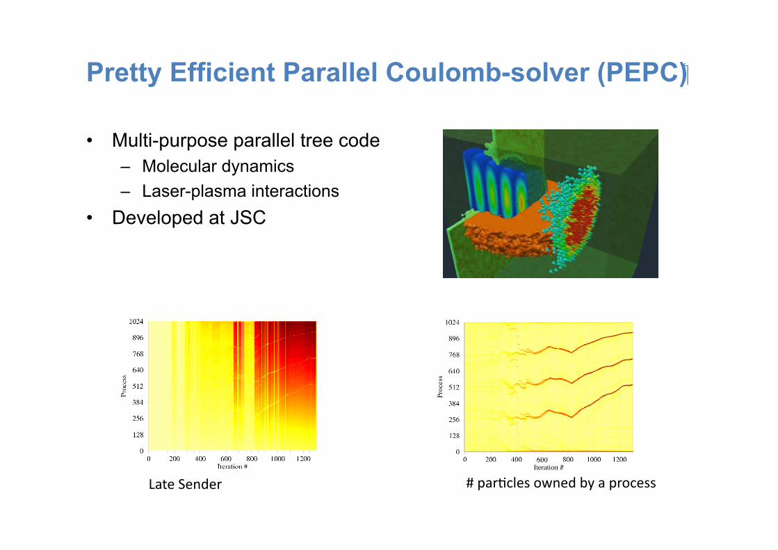
Pretty Efficient Parallel Coulomb-solver (PEPC)‏

•  Multi-purpose parallel tree code –  Molecular dynamics –  Laser-plasma interactions

•  Developed at JSC

Late  Sender   #  par:cles  owned  by  a  process  

Reconciling sampling and direct instrumentation

•  Semantic compression needs direct instrumentation to capture communication metrics and to track the call path

•  Direct instrumentation may result in excessive overhead •  New hybrid approach

–  Applies low-overhead sampling to user code –  Intercepts MPI calls via direct instrumentation –  Relies on efficient stack unwinding –  Integrates measurements in statistically sound manner

Zoltan   Szebenyi   et   al.:   Reconciling   sampling   and   direct   instrumenta:on   for  unintrusive  call-­‐path  profiling  of  MPI  programs.  In  Proc.  of  IPDPS,  Anchorage,  AK,  USA.  IEEE  Computer  Society,  May  2011.  (to  appear)    

Joint  work  with  

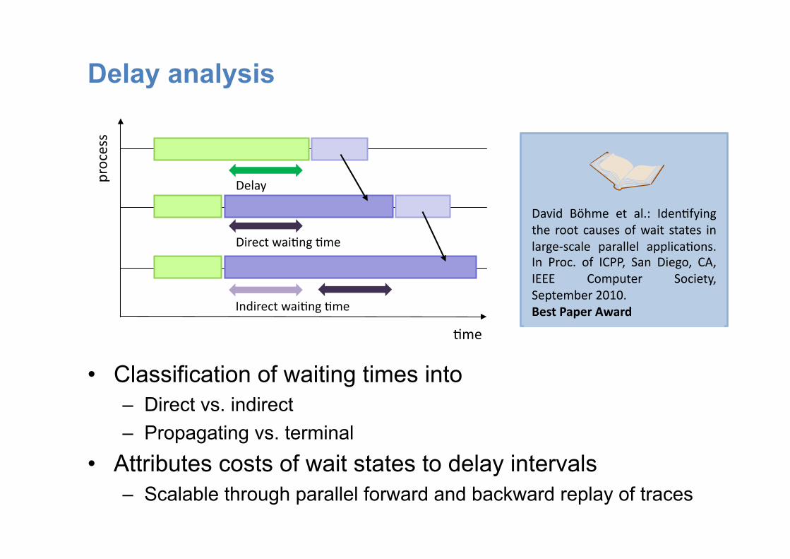
Delay analysis

•  Classification of waiting times into –  Direct vs. indirect –  Propagating vs. terminal

•  Attributes costs of wait states to delay intervals –  Scalable through parallel forward and backward replay of traces

:me  

process  

Delay  

Direct  wai:ng  :me  

   Indirect  wai:ng  :me    

David   Böhme   et   al.:   Iden:fying  the   root   causes  of  wait   states   in  large-­‐scale   parallel   applica:ons.  In   Proc.   of   ICPP,   San   Diego,   CA,  IEEE   Computer   Society,  September  2010.    Best  Paper  Award  

Delay analysis of code Illumination

•  Particle physics code (laser-plasma interaction) •  Delay analysis identified inefficient communication

behavior as cause of wait states

Computa:on     Propaga:ng  wait  states:  Original  vs.  op:mized  code  

Costs  of  direct  delay  in  op:mized  code  

Score-P measurement system

Applica:on  (MPI,  OpenMP,  accelerator,  PGAS,  hybrid)  

Score-­‐P  measurement  infrastructure  

Online  interface  Profiling  Tracing  

Interac:ve  trace  

explora:on  

Vampir  Performance  dynamics  &  wait  states  

Scalasca  Automa:c  online  

classifica:on  

Periscope  Performance  data  base  &  data  mining  

TAU  

Future work

•  Further scalability improvements •  Emerging architectures and programming models

–  PGAS languages –  Accelerator architectures

•  Interoperability with 3rd-party tools –  Common measurement library for several performance tools

Virtual Institute – High Productivity Supercomputing

The virtual institute in a… •  Partnership to develop advanced programming tools for complex simulation codes

•  Goals •  Improve code quality •  Speed up development

•  Activities •  Tool development and

integration •  Training •  Support •  Academic workshops

•  www.vi-hps.org

Thank you!