METHODS FOR THE QUANTIFICATION OF AIRCRAFT LOADS IN DLR-PROJECT ILOADS

Sunpeth Cumnuantip1, Thiemo Kier2, Kristof Risse3 and Gabriel P. Chiozzotto1

German Aerospace Center (DLR) 1Institute of Aeroelasticity, 2Institute of System Dynamics and Control, 3Institute of Aerodynamics

and Flow Technology

Abstract

This work presents the assessment of the methods for the quantification of aircraft loads within the second work package, “Methods for the Quantification of Aircraft Loads”, in the German Aerospace Center (DLR) project, iLOADS. This paper assesses and compares different aircraft loads analysis methods with different levels of complexity. Three topics relevant for aircraft loads analysis are addressed in this paper: aerodynamic methods for aircraft loads analysis, dynamic loads analysis methods and effects of the aircraft controls on the aircraft loads. These disciplines are analyzed both for the whole aircraft design level and for an aircraft component design level. Results from these analyses are compared with reference data. An important result of the work is information on the precision and conservativeness of the loads result from each of these approaches. 1. INTRODUCTION

An aircraft loads determination is one of the important disciplines during an aircraft design. Aircraft loads analysis serves as the major input for the aircraft structural dimensioning and for the proof of the aircraft safety such as during the certification process the maximum aircraft loads must not exceed the maximum allowable loads.

The German Aerospace Center, DLR, has certain experience in different projects concerned with aircraft design and assessment. DLR also has its own research aircraft fleet [1] such as the HALO, operated by DLR, and and the DLR FALCON, where the installation of DLR specific external research instruments must be certified. These activities require the fundamental knowledge on the aircraft loads analysis process both for the aircraft design and for the aircraft instrument certification. Various DLR institutes have contributed their knowledge in this discipline into these activities. This paper describes the DLR capability in this field. It assesses the state of the art methods with different levels of complexity that are implemented by DLR institutes during the process of the above mentioned projects.

The first section of this paper focuses on the aerodynamic methods. Various Euler-based methods, e.g. a linear-potential method and a full potential method are compared for the aerodynamic loads analysis of the DLR D150 transport aircraft. The distributed and the concentrated span-wise load distribution are the major result of interest for the comparison. The second section is concerned with the aircraft dynamic loads analysis. Methods for gust loads analysis and ground loads determination are evaluated. The Pratt’s (quasi-static) method [2] is verified for a special test case of a simplified wing fulfilling Pratt’s assumptions. Results for the Pratt approach are compared with a fully dynamic gust loads analysis method (within MSC NASTRAN) for the DLR D150 reference aircraft. In the case of the ground loads analysis, an empirical method and the multibody simulation method, MBS, are compared for the determination of ground loads of the

VFW 614 reference aircraft. The third section describes the analysis of the effect of a flight control system on dynamic loads. The focus is on the analysis of the lateral dynamic maneuver loads. The effect of the control surface deflections and their dependence on control parameters, e.g. yaw-damper parameters on the dynamic loads of the vertical tailplane is investigated.

Finally, the result of this paper will serve as fundamental information for the implementation of the proper aircraft loads analysis process and methods that suit the requirement of different aircraft design phases and certification.

2. AERODYNAMIC LOADS ANALYSIS METHOD

In the iLOADS project, systematic aerodynamic simulations have been performed for short range reference aircraft configuration. Methods and tools of different fidelity levels have been used for varying input parameters, aircraft configurations and flight conditions to analyse applicability limits and prediction accuracies for aerodynamic characteristics with specific focus on subsequent loads analyses. The discussion herein therefore focuses on the prediction and comparison of spanwise distributions of aerodynamic coefficients and their gradients with respect to the angle of attack.

2.1. Reference Configuration

The reference aircraft configuration used for the aerodynamic simulations is based on the DLR D150, which has similar characteristics as an Airbus A320. To allow transonic 3D flow computations using Euler- or Navier-Stokes-based methods, the 3D wing shape of the DLR-F6 configuration is used [9], while fuselage and tails have been manually adapted to the D150 configuration. The new configuration is called D150-F6. The CAD geometry has also been exported to the standardized DLR XML file format CPACS [10].

Deutscher Luft- und Raumfahrtkongress 2016DocumentID: 420145

1©2016

2.2. Aerodynamic Simulations

Different aerodynamic methods and programs have been compared during the iLOADS project, from which the following three are presented within this paper:

• LIFTING_LINE (multi-lifting-line code) [11], [12] • VSAERO (3D panel code) [13] • TAU (3D RANS1 solver) [14]

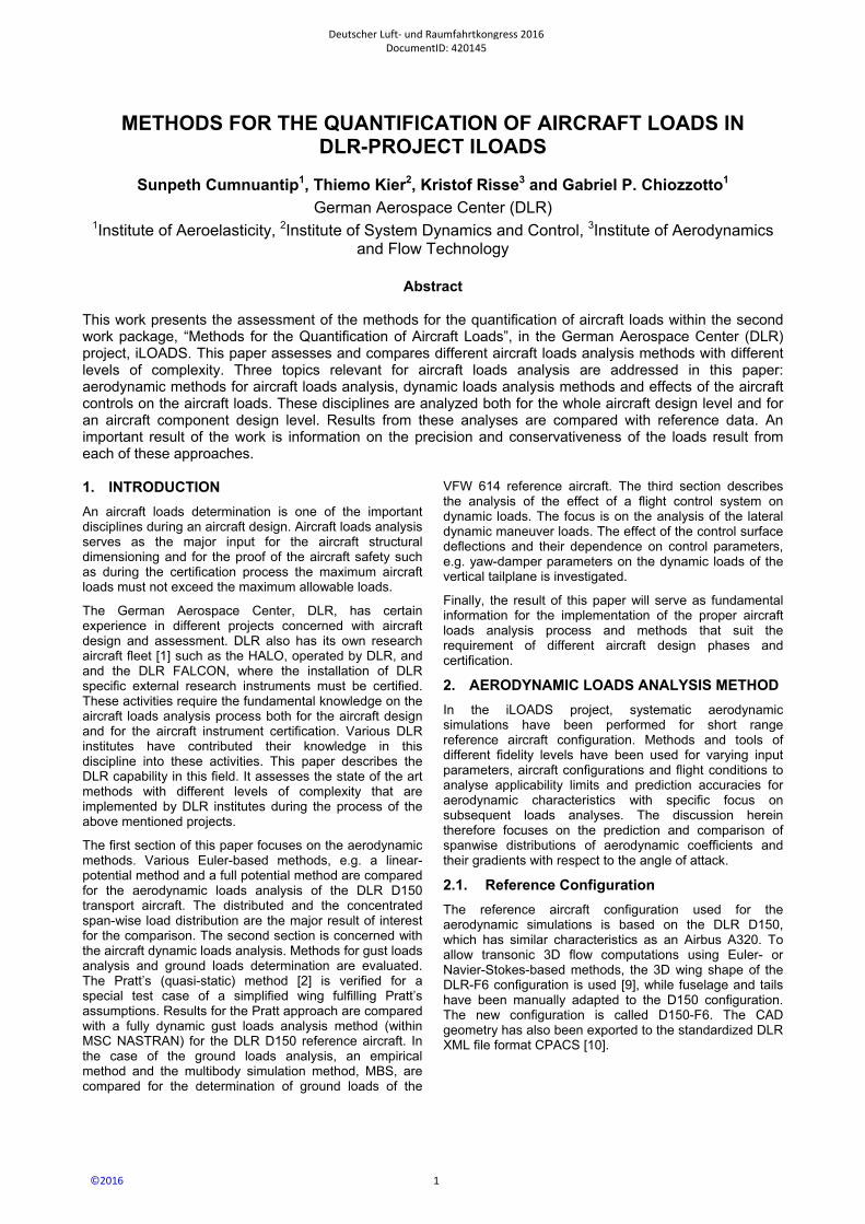
For LIFTING_LINE and VSAERO, tool wrappers based on the DLR CPACS format are used that are being developed at the DLR Institute of Aerodynamics and Flow Technology (DLR-AS). It has to be noted that in their current version, the wrappers model only wing and tail geometries, i.e. the aerodynamic influence of the fuselage is neglected. For the LIFTING_LINE and VSAERO CPACS wrappers, systematic variations of panel number and surface distribution in chord- and spanwise directions have been performed first to derive suitable parameter settings. While the distribution of local lift coefficients Cl converges already for small panel numbers, the sensitivity of the local pitching moment coefficient Cmy towards wing panelling is significantly stronger, which is mainly due to the changes in the local centre of pressure.

For the derived panel settings, Figure 1 shows the spanwise distribution of Cl as well as its local gradients with respect to the total angle of attack αtot at the transonic Mach number M = 0.75. The small absolute deviations also confirm the agreement of the (subsonic) compressibility corrections implemented in both tools. The good agreement for the Cl gradients could also be shown for wing-tail configurations, and only changed marginally with selection of different reference values to compute the gradients.

Figure 1: Comparison of Cl distributions between LIFTING_LINE (LILI) and VSAERO (VSA)

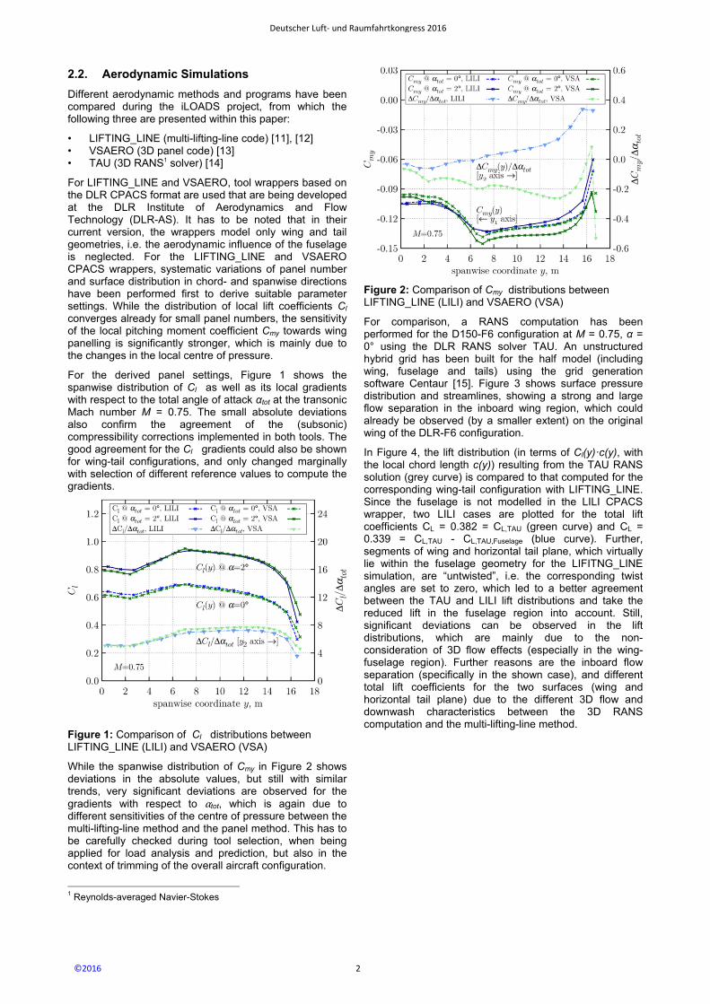
While the spanwise distribution of Cmy in Figure 2 shows deviations in the absolute values, but still with similar trends, very significant deviations are observed for the gradients with respect to ⍺tot, which is again due to different sensitivities of the centre of pressure between the multi-lifting-line method and the panel method. This has to be carefully checked during tool selection, when being applied for load analysis and prediction, but also in the context of trimming of the overall aircraft configuration.

1 Reynolds-averaged Navier-Stokes

Figure 2: Comparison of Cmy distributions between LIFTING_LINE (LILI) and VSAERO (VSA)

For comparison, a RANS computation has been performed for the D150-F6 configuration at M = 0.75, α = 0° using the DLR RANS solver TAU. An unstructured hybrid grid has been built for the half model (including wing, fuselage and tails) using the grid generation software Centaur [15]. Figure 3 shows surface pressure distribution and streamlines, showing a strong and large flow separation in the inboard wing region, which could already be observed (by a smaller extent) on the original wing of the DLR-F6 configuration.

In Figure 4, the lift distribution (in terms of Cl(y)·c(y), with the local chord length c(y)) resulting from the TAU RANS solution (grey curve) is compared to that computed for the corresponding wing-tail configuration with LIFTING_LINE. Since the fuselage is not modelled in the LILI CPACS wrapper, two LILI cases are plotted for the total lift coefficients CL = 0.382 = CL,TAU (green curve) and CL = 0.339 = CL,TAU - CL,TAU,Fuselage (blue curve). Further, segments of wing and horizontal tail plane, which virtually lie within the fuselage geometry for the LIFITNG_LINE simulation, are “untwisted”, i.e. the corresponding twist angles are set to zero, which led to a better agreement between the TAU and LILI lift distributions and take the reduced lift in the fuselage region into account. Still, significant deviations can be observed in the lift distributions, which are mainly due to the non-consideration of 3D flow effects (especially in the wing-fuselage region). Further reasons are the inboard flow separation (specifically in the shown case), and different total lift coefficients for the two surfaces (wing and horizontal tail plane) due to the different 3D flow and downwash characteristics between the 3D RANS computation and the multi-lifting-line method.

Deutscher Luft- und Raumfahrtkongress 2016

2©2016

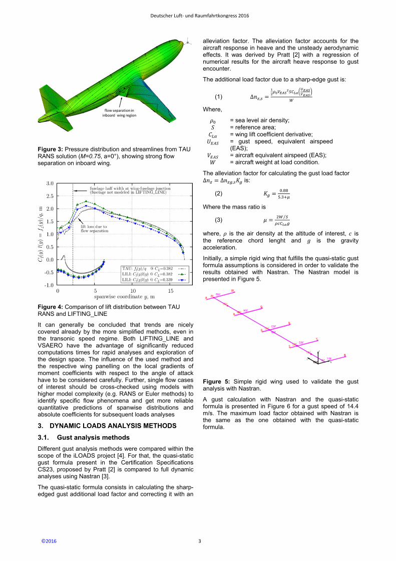
Figure 3: Pressure distribution and streamlines from TAU RANS solution (M=0.75, a=0°), showing strong flow separation on inboard wing.

Figure 4: Comparison of lift distribution between TAU RANS and LIFTING_LINE

It can generally be concluded that trends are nicely covered already by the more simplified methods, even in the transonic speed regime. Both LIFTING_LINE and VSAERO have the advantage of significantly reduced computations times for rapid analyses and exploration of the design space. The influence of the used method and the respective wing panelling on the local gradients of moment coefficients with respect to the angle of attack have to be considered carefully. Further, single flow cases of interest should be cross-checked using models with higher model complexity (e.g. RANS or Euler methods) to identify specific flow phenomena and get more reliable quantitative predictions of spanwise distributions and absolute coefficients for subsequent loads analyses

3. DYNAMIC LOADS ANALYSIS METHODS

3.1. Gust analysis methods

Different gust analysis methods were compared within the scope of the iLOADS project [4]. For that, the quasi-static gust formula present in the Certification Specifications CS23, proposed by Pratt [2] is compared to full dynamic analyses using Nastran [3].

The quasi-static formula consists in calculating the sharp-edged gust additional load factor and correcting it with an

alleviation factor. The alleviation factor accounts for the aircraft response in heave and the unsteady aerodynamic effects. It was derived by Pratt [2] with a regression of numerical results for the aircraft heave response to gust encounter.

The additional load factor due to a sharp-edge gust is:

(1) ∆ ,

Where,

= sea level air density; = reference area; = wing lift coefficient derivative; = gust speed, equivalent airspeed

(EAS); = aircraft equivalent airspeed (EAS);

= aircraft weight at load condition.

The alleviation factor for calculating the gust load factor ∆ ∆ , is:

(2) .

.

Where the mass ratio is

(3) ⁄

where, is the air density at the altitude of interest, is the reference chord lenght and is the gravity acceleration.

Initially, a simple rigid wing that fulfills the quasi-static gust formula assumptions is considered in order to validate the results obtained with Nastran. The Nastran model is presented in Figure 5.

Figure 5: Simple rigid wing used to validate the gust analysis with Nastran.

A gust calculation with Nastran and the quasi-static formula is presented in Figure 6 for a gust speed of 14.4 m/s. The maximum load factor obtained with Nastran is the same as the one obtained with the quasi-static formula.

Deutscher Luft- und Raumfahrtkongress 2016

3©2016

Figure 6: Gust response for simple rigid wing comparison between Nastran dynamic results and quasi-static gust formula.

A short-range aircraft for 150 passengers, D150, was used as a representative configuration to perform detailed gust analyses. The aircraft Nastran model is shown in Figure 7.

Figure 7: D150 model used for gust analysis.

The gust response results for a selected mass case at three different altitudes and different gust lengths are shown in Figure 8. There is a good agreement between the Nastran dynamic response and the quasi-static formula (dashed line) results.

Figure 8: D150 gust response results for different altitudes and gust lengths. Comparison between Nastran dynamic results and quasi-static formula.

Several load cases for different mass cases, altitudes, design speeds and gust lengths have been considered to calculate the aircraft gust load envelope. The calculations were performed with the dynamic Nastran solution and the quasi-static formula. The results are presented in Figure 9 for the wing bending and in Figure 10 for the wing torsion envelopes. The bending envelopes are very similar for both methods but some differences appear in the torsional load envelope inboard of the engine attachment. The differences are likely caused by the dynamic response of the aircraft in other degrees-of-freedom different than the heave motion, e.g. aircraft pitching acceleration and wing flexible modes.

Figure 9: D150 gust bending moment at the wing load reference axis envelope.

Deutscher Luft- und Raumfahrtkongress 2016

4©2016

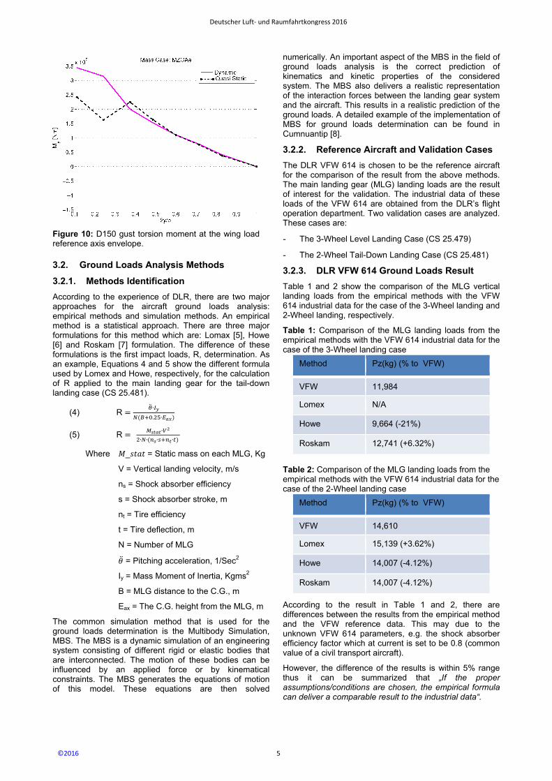
Figure 10: D150 gust torsion moment at the wing load reference axis envelope.

3.2. Ground Loads Analysis Methods

3.2.1. Methods Identification

According to the experience of DLR, there are two major approaches for the aircraft ground loads analysis: empirical methods and simulation methods. An empirical method is a statistical approach. There are three major formulations for this method which are: Lomax [5], Howe [6] and Roskam [7] formulation. The difference of these formulations is the first impact loads, R, determination. As an example, Equations 4 and 5 show the different formula used by Lomex and Howe, respectively, for the calculation of R applied to the main landing gear for the tail-down landing case (CS 25.481).

(4) R ∙

. ∙

(5) R ∙

∙ ∙ ∙ ∙

Where _ = Static mass on each MLG, Kg

V = Vertical landing velocity, m/s

ns = Shock absorber efficiency

s = Shock absorber stroke, m

nt = Tire efficiency

t = Tire deflection, m

N = Number of MLG

= Pitching acceleration, 1/Sec2

Iy = Mass Moment of Inertia, Kgms2

B = MLG distance to the C.G., m

Eax = The C.G. height from the MLG, m

The common simulation method that is used for the ground loads determination is the Multibody Simulation, MBS. The MBS is a dynamic simulation of an engineering system consisting of different rigid or elastic bodies that are interconnected. The motion of these bodies can be influenced by an applied force or by kinematical constraints. The MBS generates the equations of motion of this model. These equations are then solved

numerically. An important aspect of the MBS in the field of ground loads analysis is the correct prediction of kinematics and kinetic properties of the considered system. The MBS also delivers a realistic representation of the interaction forces between the landing gear system and the aircraft. This results in a realistic prediction of the ground loads. A detailed example of the implementation of MBS for ground loads determination can be found in Cumnuantip [8].

3.2.2. Reference Aircraft and Validation Cases

The DLR VFW 614 is chosen to be the reference aircraft for the comparison of the result from the above methods. The main landing gear (MLG) landing loads are the result of interest for the validation. The industrial data of these loads of the VFW 614 are obtained from the DLR’s flight operation department. Two validation cases are analyzed. These cases are:

- The 3-Wheel Level Landing Case (CS 25.479)

- The 2-Wheel Tail-Down Landing Case (CS 25.481)

3.2.3. DLR VFW 614 Ground Loads Result

Table 1 and 2 show the comparison of the MLG vertical landing loads from the empirical methods with the VFW 614 industrial data for the case of the 3-Wheel landing and 2-Wheel landing, respectively.

Table 1: Comparison of the MLG landing loads from the empirical methods with the VFW 614 industrial data for the case of the 3-Wheel landing case

Method Pz(kg) (% to VFW)

VFW 11,984

Lomex N/A

Howe 9,664 (-21%)

Roskam 12,741 (+6.32%)

Table 2: Comparison of the MLG landing loads from the empirical methods with the VFW 614 industrial data for the case of the 2-Wheel landing case

Method Pz(kg) (% to VFW)

VFW 14,610

Lomex 15,139 (+3.62%)

Howe 14,007 (-4.12%)

Roskam 14,007 (-4.12%)

According to the result in Table 1 and 2, there are differences between the results from the empirical method and the VFW reference data. This may due to the unknown VFW 614 parameters, e.g. the shock absorber efficiency factor which at current is set to be 0.8 (common value of a civil transport aircraft).

However, the difference of the results is within 5% range thus it can be summarized that „If the proper assumptions/conditions are chosen, the empirical formula can deliver a comparable result to the industrial data“.

Deutscher Luft- und Raumfahrtkongress 2016

5©2016

Concerning the simulation result, Figure 11 shows the comparison of the MLG vertical landing loads result from the empirical method, the simulation method and the VFW 614 reference data for the 3 Wheel-Landing case.

Figure 11: An MBS model of VFW 614 for the 3 Wheel-Landing case and the comparison of main landing gear attachment loads result from the empirical method and from the MBS

It can be observed from Figure 11 that the result from the MBS is closer to industrial data than the result from the empirical method. However, the results from both methods deliver comparable results (within 5% difference) to the reference industrial data. This can be expected for the conventional aircraft like the VFW 614 where the parameters of an empirical method are also valid.

However, for unconventional landing gear or aircraft configurations, statistical methods cannot be expected to give reliable results because of the missing data base.

4. THE EFFECT OF A FLIGHT CONTROL SYSTEM ON AIRCRAFT DYNAMIC LOADS.

All modern transport aircraft make use of an electronic flight control system. Its main purpose is to beneficially influence the flight dynamics in terms of handling qualities or preventing upset conditions. The presence of flight control laws can have a major impact on the resulting loads acting on the aircraft structure. The focus in this part of the iLOADS project was on simulating lateral dynamic manoeuvres of controlled aircraft and assessing the differences to simple trim calculations.

The dynamic simulations and trim calculations were implemented in the loads analysis environment VarLoads [17], [18]. The methods developed in the iLOADS project were also applied in other projects, e.g. in the loads process for the MDO applications [21].

4.1. The Yaw Manoeuvre

The yaw manoeuvre is described in paragraph CS 25.351 of the regulations [20]. This manoeuvre is usually the dimensioning load condition for the Vertical Tail Plane (VTP). It can be characterized by four different phases:

1. “Onset”: Starting from level flight, the rudder is deflected by a sudden pilot pedal command.

2. “Overswing”: As a result of the rudder command the aircraft starts to yaw and a dynamic overswing resulting in a maximum sideslip angle occurs.

3. “Equilibrium Yaw”: Continuing the full rudder command, a state of constant sideslip is reached.

4. “Rudder Return”: Form the steady sideslip condition, the rudder command is returned to zero.

The individual phases are illustrated in Figure 11

Figure 12: Yaw manoeuvre according to CS 25.351

4.1.1. Controller for Yaw Damping

The yaw manoeuvre is heavily influenced by the characteristics of the yaw damper function of the flight control system. The main purpose of this function is to damp out the unfavorable flight mechanical dutch roll mode. A so called rudder travel limitation unit (RTLU), reduces the maximum possible control surface deflection scheduled with airspeed in order to avoid excessive loads. Further a controller function acting as pilot model is employed to keep the wings level during the manoeuvre by using the ailerons to counter act the induced rolling moment. A cascading controller implementation according to [16] was chosen. The yaw damper function includes a parameter k which can be used to adjust the degree of damping. A value of k=0 corresponds to the undamped case.

4.1.2. Dynamic Yaw Simulations

To illustrate the influence of the control law of the yaw damper, a parametric study was carried out varying the parameter k between 0 (undamped) and 2 (highly damped).

A time series of the closed loop dynamic simulation for a moderately damped case (k=0.5) is depicted in Figure 13. The pilot command is a step input in the rudder pedals. The resulting rudder deflection r and the resulting sideslip angle are depicted in the lower left graph of Figure 13. The influence of the yaw damper control function and the RTLU are clearly visible. The bending (upper left) and torsion (lower right) loads of the VTP root are aggregated in the so called correlated loads (upper right), which is sometimes referred to as “potato” plot. The convex hull determines the critical loads. This is the so called loads envelope and the structure has to be designed accordingly.

Deutscher Luft- und Raumfahrtkongress 2016

6©2016

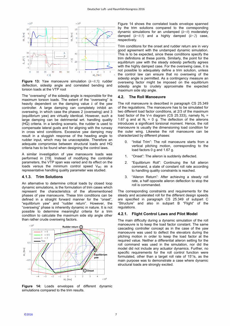
Figure 13: Yaw manoeuvre simulation (k=0.5): rudder deflection, sideslip angle and correlated bending and torsion loads at the VTP root

The “overswing” of the sideslip angle is responsible for the maximum torsion loads. The extent of the “overswing” is heavily dependent on the damping value k of the yaw controller. A large damping can completely inhibit an overswing, in which case the phases 2 (overswing) and 3 (equilibrium yaw) are virtually identical. However, such a large damping can be detrimental wrt. handling quality (HQ) criteria. In a landing scenario, the rudder is used to compensate lateral gusts and for aligning with the runway in cross wind conditions. Excessive yaw damping may result in a sluggish response of the heading angle to rudder input, which may be unacceptable. Therefore an adequate compromise between structural loads and HQ criteria has to be found when designing the control laws.

A similar investigation of yaw manoeuvre loads was performed in [19]. Instead of modifying the controller parameters, the VTP span was varied and its effect on the loads versus the minimum control speed VMC as a representative handling quality parameter was studied.

4.1.3. Trim Solutions

An alternative to determine critical loads by closed loop dynamic simulations, is the formulation of trim cases which represent the characteristics of the aforementioned phases of yaw manoeuvre. These trim conditions can be defined in a straight forward manner for the “onset”, “equilibrium yaw” and “rudder return”. However, the “overswing” phase is inherently dynamic in nature. It is not possible to determine meaningful criteria for a trim condition to calculate the maximum side slip angle other than rather crude overswing factors.

Figure 14: Loads envelopes of different dynamic simulations compared to the trim results.

Figure 14 shows the correlated loads envelope spanned by the trim solutions compared to the corresponding dynamic simulations for an undamped (k=0) moderately damped (k=0.5) and a highly damped (k=2) case, respectively.

Trim conditions for the onset and rudder return are in very good agreement with the undamped dynamic simulation. This is to be expected, since these conditions specify the trim definitions at these points. Similarly, the point for the equilibrium yaw with the steady sideslip perfectly agrees with the highly damped case. For the overswing case, it is not possible to adequately define a trim solution, unless the control law can ensure that no overswing of the sideslip angle is permitted. As a contingency measure an overswing factor might be imposed on the equilibrium sideslip angle to crudely approximate the expected maximum side slip angle.

4.2. The Roll Manoeuvre

The roll manoeuvre is described in paragraph CS 25.349 of the regulations. The manoeuvre has to be simulated for two different load factor conditions, at 2/3 of the maximum load factor of the V-n diagram (CS 25.333), namely Nz = 1.67 g and at Nz = 0 g. The deflection of the ailerons introduces a significant torsional moment. Hence, the roll manoeuvre is usually the dimensioning load condition for the outer wing. Likewise the roll manoeuvre can be characterized by different phases:

0. “Initial Trim”: The roll manoeuvre starts from a vertical pitching motion, corresponding to the load factors 0 g and 1.67 g.

1. “Onset”: The aileron is suddenly deflected.

2. “Equilibrium Roll”: Continuing the full aileron command, a state of constant roll rate according to handling quality constraints is reached.

3. “Aileron Return”: After achieving a steady roll rate, a half opposite aileron deflection to stop the roll is commanded.

The corresponding constraints and requirements for the steady and accelerated roll for the different design speeds are specified in paragraph CS 25.349 of subpart C “Structure” and also in subpart B “Flight” of the regulations.

4.2.1. Flight Control Laws and Pilot Model

The main difficulty during a dynamic simulation of the roll manoeuvre is to keep the load factor constant. The same cascading controller concept as in the case of the yaw manoeuvre was used to deflect the elevators during the pitching motion in order to keep the load factor at the required value. Neither a differential aileron setting for the roll command was used in the simulation, nor did the model did not include any actuator dynamics. Further, no specific requirements for the roll control function were formulated, other than a target roll rate of 15°/s, as the main purpose was to demonstrate a case where dynamic structural loads are strongly excited.

Deutscher Luft- und Raumfahrtkongress 2016

7©2016

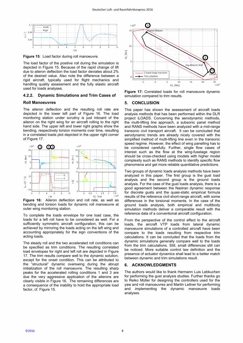
Figure 15: Load factor during roll manoeuvre.

The load factor of the positive roll during the simulation is depicted in Figure 15. Because of the rapid change of lift due to aileron deflection the load factor deviates about 2% of the desired value. Also note the difference between a rigid aircraft, typically used for flight mechanics and handling quality assessment and the fully elastic aircraft used for loads analyses.

4.2.2. Dynamic Simulations and Trim Cases of

Roll Manoeuvres

The aileron deflection and the resulting roll rate are depicted in the lower left part of Figure 16. The load monitoring station under scrutiny is just inboard of the aileron on the right wing for an aircraft rolling to the right hand side. The upper left and lower right graphs show the bending, respectively torsion moments over time, resulting in a correlated loads plot depicted in the upper right corner of Figure 17.

Figure 16: Aileron deflection and roll rate, as well as bending and torsion loads for dynamic roll manoeuvre at outer wing monitoring station.

To complete the loads envelope for one load case, the loads for a left roll have to be considered as well. For a sufficiently symmetric aircraft configuration, this can be achieved by mirroring the loads acting on the left wing and accounting appropriately for the sign conventions of the acting loads.

The steady roll and the two accelerated roll conditions can be specified as trim conditions. The resulting correlated load envelopes for right and left roll are depicted in Figure 17. The trim results compare well to the dynamic solution, except for the onset condition. This can be attributed to the “structural” dynamic overswing during the abrupt initialization of the roll manoeuvre. The resulting sharp peaks for the accelerated rolling conditions 1 and 3 are due the very aggressive application of the ailerons are clearly visible in Figure 16. The remaining differences are a consequence of the inability to hold the appropriate load factor, cf. Figure 15.

Figure 17: Correlated loads for roll manoeuvre dynamic simulation compared to trim results.

5. CONCLUSION

This paper has shown the assessment of aircraft loads analysis methods that has been performed within the DLR project iLOADS. Concerning the aerodynamic methods, the multi-lifting line approach, a subsonic panel method and RANS methods have been analyzed with a mid-range transonic civil transport aircraft. It can be concluded that aerodynamic trends are already nicely covered with the simplified method of multi-lifting line even in the transonic speed regime. However, the effect of wing panelling has to be considered carefully. Further, single flow cases of interest such as the flow at the wing-fuselage region should be cross-checked using models with higher model complexity such as RANS methods to identify specific flow phenomena and get more reliable quantitative predictions.

Two groups of dynamic loads analysis methods have been analyzed in this paper. The first group is the gust load analysis and the second group is the ground loads analysis. For the case of the gust loads analysis, there is a good agreement between the Nastran dynamic response for discrete gusts and the quasi-static empirical formula results of the reference civil short-range aircraft, with some differences in the torsional moments. In the case of the ground loads analysis, both empirical and multibody simulation methods deliver a comparable result with the reference data of a conventional aircraft configuration.

From the perspective of the control effect to the aircraft loads, the aircraft VTP loads from lateral dynamic manoeuvre simulations of a controlled aircraft have been compare to the loads resulting from respective trim calculations. It can be concluded that the loads from the dynamic simulations generally compare well to the loads from the trim calculations. Still, small differences still can be noticed. More suitable control law definition and the presence of actuator dynamics shall lead to a better match between dynamic and trim simulations result.

6. ACKNOWLEDGMENTS

The authors would like to thank Hermann Luis Lebkuchen for performing the gust analysis studies. Further thanks go to Reiko Müller for designing the controllers used for the yaw and roll manoeuvres and Martin Leitner for performing and implementing the dynamic manoeuvre loads analyses.

Deutscher Luft- und Raumfahrtkongress 2016

8©2016

7. REFERENCES

1. DLR-Flugzeugflotte: http:// http://www.dlr.de/dlr/ desktopdefault.aspx/tabid-10203/. Last visited 11.09, 2016.

2. Pratt, K. G., A revised formula for the calculation of gust loads. NACA TN-2964, 1953.

3. MSC Software Corporation: MSC.Nastran Version 68

– Aeroelastic Analysis User's Guide. 2004. 4. Lebkuchen, L. H., „Gust Loads Analysis on a Civil

Transport Airliner“, IB 232-2015 J 12, DLR, Göttingen, 2015.

5. Lomax, L. Ted., Structural Loads Analysis for

Commercial Transport Aircraft: Theory and Practice. AIAA Education Series, Washington, 1995.

6. Howe, D., Aircraft Loading and Structural Layout.

Professional Engineering Publishing, United Kingdom, 2004.

7. Roskam, J., Airplane Design Part IV: Layout Design

of Landing Gear and Systems. Roskam Aviation and Engineering Corporation, Kansas, 1986.

8. Cumnuantip, S., Landing Gear Positioning and

Structural Mass Optimization for a Large Blended Wing Body Aircraft. PhD Thesis. Technical University of Munich, Germany, 2014.

9. Brodersen, O., “Drag Prediction of Engine-Airframe

Interference Effects Using Unstructured Navier-Stokes Calculations, Journal of Aircraft, Vol. 39, No. 6, 2002.

10. German Aerospace Center (DLR): CPACS—A

Common Language for Aircraft Design (2014). https://software.dlr.de/p/cpacs/home/

11. Horstmann, K.-H., “Ein Mehrfach-Traglinienverfahren und seine Verwendung für Entwurf und Nachrechnung nichtplanarer Flügelanordnungen”, Ph.D. Dissertation, Technical University of Braunschweig, Braunschweig, Germany, 1987; see also: Tech. Rep. FB 87-51, DFVLR, Braunschweig, Germany, 1987.

12. Horstmann, K.-H., Engelbrecht, T., and Liersch, C.

M., “LIFTING_LINE v2.3 Handbook [user guide]”, DLR Institute of Aerodynamics and Flow Technology, Braunschweig, Germany, 2010.

13. Analytical Methods, “VSERO – A Code for Calculating

the Nonlinear Aerodynaimc Characteristics of Arbitrary ConFigureruation”, User’s Manual Version 7.2, Redmond, WA, 2007.

14. Gerhold, T., “Overview of the Hybrid RANS Code

TAU,” MEGAFLOW—Numerical Flow Simulation for Aircraft Design, edited by Kroll, N. and Fassbender, J. K., Vol. 89 of Notes on Numerical Fluid Mechanics and Multidisciplinary Design, Springer, Berlin and Heidelberg, Germany, 2005, pp. 81–92.

15. CentaurSoft, “CENTAUR: Mesh (Grid) Generation for CFD and Computational Simulations [Software],” CentaurSoft, Austin, TX. URL: https://www.centaursoft.com.

16. Brockhaus, R., Alles, W. and Luckner, R. „Flugregelung“. Springer, 2011.

17. Hofstee, J., Kier, T., Cerulli, C. and Looye, G., “A variable, fully flexible dynamic response tool for special investigations (VarLoads),” International Forum on Aeroelasticity and Structural Dynamics, 2003.

18. Kier, T. and Hofstee, J., „VarLoads - eine Simulations-

umgebung zur Lastenberechnung eines voll flexible, freifliegenden Flugzeugs“, Deutscher Luft- und Raumfahrtkongress, 2004.

19. Kier, T., Looye, G. and Hofstee, J., “Development of

Aircraft Flight Loads Analysis Models with Uncertainties for Pre-Design Studies”, International Forum on Aeroelasticity and Structural Dynamics, 2005.

20. European Aviation Safety Agency, “Certification

Specifications and Acceptable Means of Compliance for Large Aeroplanes, CS-25,” 2015.

21. Leitner, M., Liepelt, R., Kier, T., Klimmek, T., Müller,

R. and Schulze, M., „A Fully Automatic Structural Optimization Framework to Determine Critical Design Loads”, Deutscher Luft- und Raumfahrtkongress, 2016.

Deutscher Luft- und Raumfahrtkongress 2016

9©2016