Embed Size (px)
Citation preview
17
Methods for Transient Stability AnalysisAnalyzing the stability of a power system as a nonlinear system modeled by DAEs (differential-algebraic equations) or DEs (differential equations) under a large disturbance.
where x are u are respectively the vectors of the state and non-state variables
• Direct methods, based on Lyapunov’s 2nd method, judge stability without solving the DAEs or DEs explicitly. One example is the EAC method for SMIB:
1. Define Transient Energy Function V(x) =Vpe+Vke (=|A1|+|A3| for SMIB)2. The system is considered stable if V(x) critical energy Vcr (=|A2|+|A3| for SMIB)
• Numerical methods (time-domain simulation) solves an Initial Value Problem of the nonlinear DAEs or DEs with known initial values x(t0)=x0 by step-by-step numerical integrations– The objective is to solve x as a function of time t.– There are two types of integration methods: explicit and implicit
( ) DEs
0 ( ) AEs
d fdt
g
x = x,u
= x,u
( ( DEs ))d fdtx = x,u x
If u can be solved as u(x) and then
eliminated
18
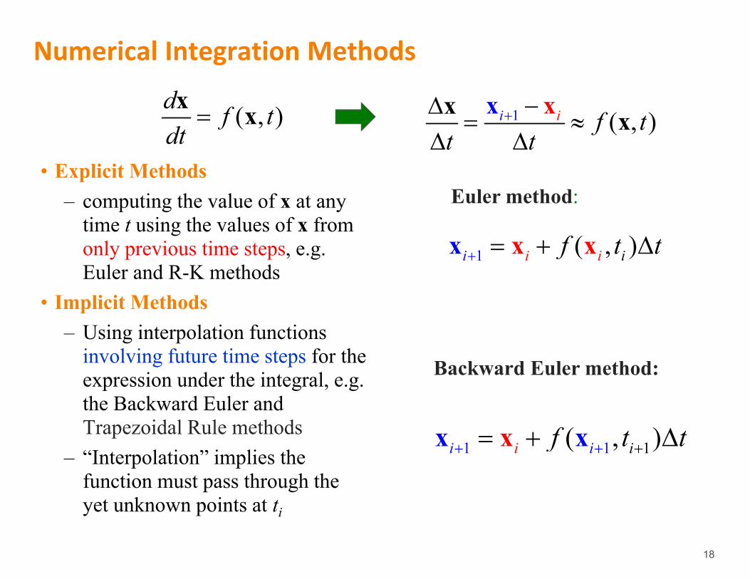
• Explicit Methods– computing the value of x at any
time t using the values of x from only previous time steps, e.g. Euler and R-K methods
• Implicit Methods– Using interpolation functions
involving future time steps for the expression under the integral, e.g. the Backward Euler and Trapezoidal Rule methods
– “Interpolation” implies the function must pass through the yet unknown points at ti
Numerical Integration Methods
( , )x xd f tdt
1 ( , )ii ii f t t x xx
1 1 1( , )i ii if t t xx x
Euler method:
Backward Euler method:
1 ( , )i i f tt t
x xxx
19
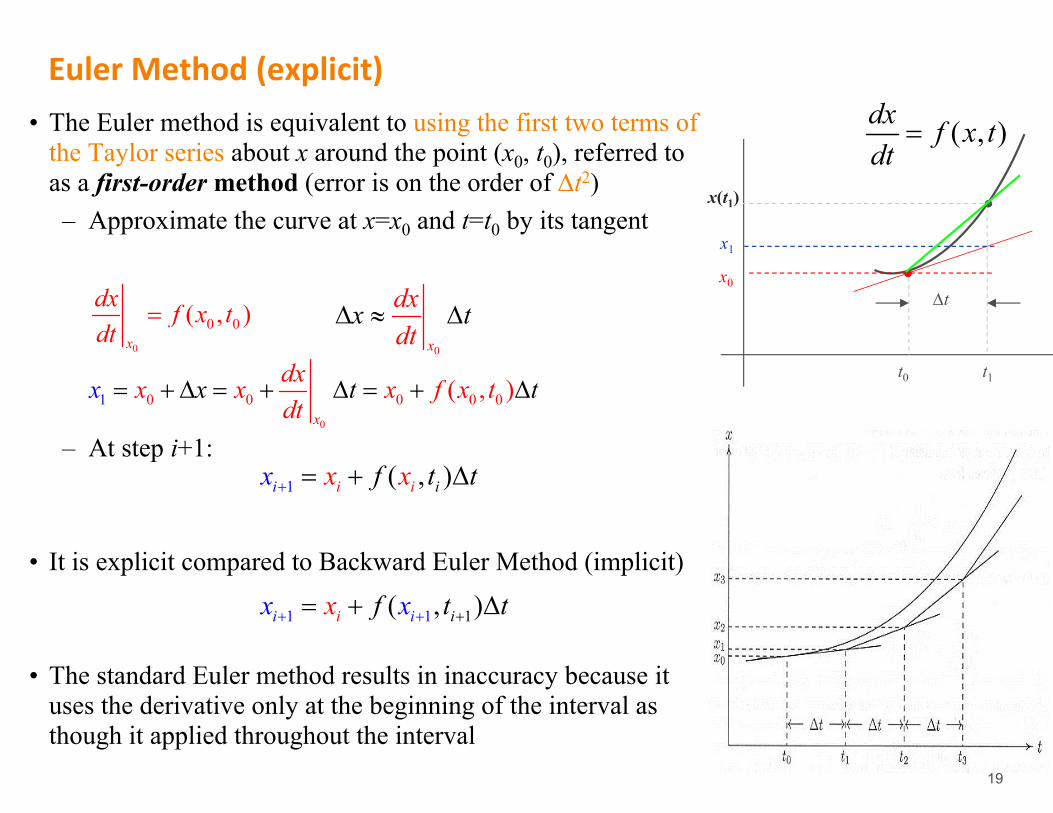
Euler Method (explicit)• The Euler method is equivalent to using the first two terms of
the Taylor series about x around the point (x0, t0), referred to as a first-order method (error is on the order of t2)– Approximate the curve at x=x0 and t=t0 by its tangent
– At step i+1:
• It is explicit compared to Backward Euler Method (implicit)
• The standard Euler method results in inaccuracy because it uses the derivative only at the beginning of the interval as though it applied throughout the interval
0
0 0( , )x
dx f x tdt
( , )dx f x tdt
0
0 0 0 0 01 ( , )x
x dxx x x f x td
x t tt
0x
dxd
xt
t
1 ( , )ii i ix x tx f t
t0 t1
x0t
x1
x(t1)
1 1 1( , )i ii if t tx x x

20
Modified Euler (ME) Method (explicit)
• Modified Euler method consists of two steps:(a) Predictor step:
The derivative at the end of the t is estimated using x1p
(b) Corrector step:
• It is a second-order method (error is on the order of t3)
0
1 0 0 0 0( , )x
p tdxx x f x tdt
x t
1
1
1( , )px
pf xdxt
td
0 1
1 0 00 0 1 1( , ) ( , )
2 2
p px xc
dx dxdt
x tdt f x t f tx x x t
1
1 1( , ) ( , )2i
pc i i i i
if x t f x tx x t
t0 t1
x0t
x1p
x1c
x (t1)
( , )dx f x tdt
Slope at the beginning of t
Estimated slope at the end of t
• Step size t must be small enough to obtain a reasonably accurate solution, but at the same time, large enough to avoid the numerical instability with the computer.
21
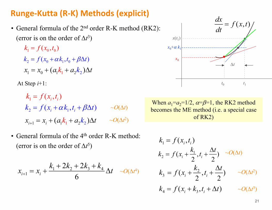
Runge‐Kutta (R‐K) Methods (explicit)
• General formula of the 2nd order R-K method (RK2): (error is on the order of t3)
• General formula of the 4th order R-K method:(error is on the order of t5)
1 1 1 2 2( )i i kx kx a a t
1 ( , )i ik f x t
2 1( , )i ik f x k t t
1 1 1 20 2( )k kx x a a t
1 0 0( , )k f x t
2 0 1 0( , )k f x k t t
When a1=a2=1/2, ==1, the RK2 method becomes the ME method (i.e. a special case
of RK2)
t0 t1
x0t
x0+ k1
( , )dx f x tdt
x(t1)
At Step i+1:
1 2 3 41
2 26i i
k k k kx x t
1 ( , )i ik f x t1
2 ( , )2 2i ik tk f x t
23 ( , )
2 2i ik tk f x t
4 3( , )i ik f x k t t
~O(t2)
~O(t)
~O(t2)
~O(t3)
~O(t4)
~O(t)
22
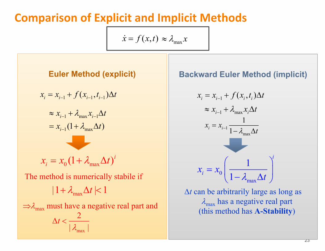
Numerical Stability of Explicit Integration Methods
• Numerical stability is related to the stiffness of the set of differential equations representing the system
• The stiffness is measured by the ratio of the largest to smallest time constant, or more precisely by |max/min| of the linearized system.
• Stiffness in a transient stability simulation increases with more details (more smaller time constants) being modeled.
• Explicit integration methods have weak stability numerically; with stiff systems, the solution “blows up” unless a small step size is used. Even after the fast modes die out, small time steps continue to be required to maintain numerical stability
23
Backward Euler Method (implicit)
t can be arbitrarily large as long as max has a negative real part
(this method has A-Stability)
Euler Method (explicit)
The method is numerically stabile if
max must have a negative real part and
Comparison of Explicit and Implicit Methods
1 1 1( , )i i i ix x f x t t
( , )x f x t
1 ( , )i i i ix x f x t t
maxx
1 max 1
1 max(1 )i i
i
x x tx t
1 maxi ix x t
1max
11i ix x
t
0 max(1 )iix x t 0
max
11
i
ix xt
max|1 | 1 t
max
2| |
t
24
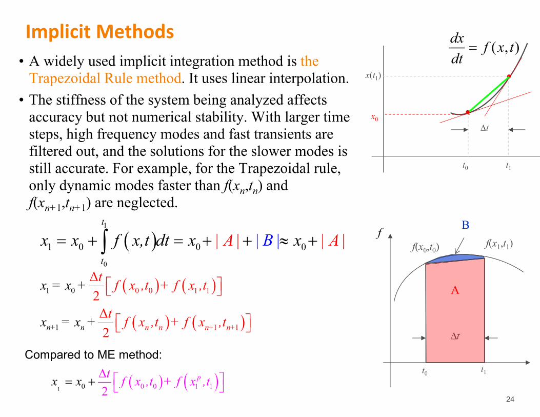
Implicit Methods• A widely used implicit integration method is the
Trapezoidal Rule method. It uses linear interpolation.• The stiffness of the system being analyzed affects
accuracy but not numerical stability. With larger time steps, high frequency modes and fast transients are filtered out, and the solutions for the slower modes is still accurate. For example, for the Trapezoidal rule, only dynamic modes faster than f(xn,tn) and f(xn+1,tn+1) are neglected.
1 0
1
0 0 1 1
1 1
Δ2Δ2 n n nn + n+n+
x = x +
x =
t f x ,t + f x ,t
t f x ,t +x f x+ ,t
1 0 0 10 12
pt f x ,t + f x ,x tx
Compared to ME method:t0 t1
f(x0,t0) f(x1,t1)
t
A
Bf
t0 t1
x0t
( , )dx f x tdt
x(t1)
1
0
1 0 0 0| | | || |t
t
x x f x,t dt x AxA B
25
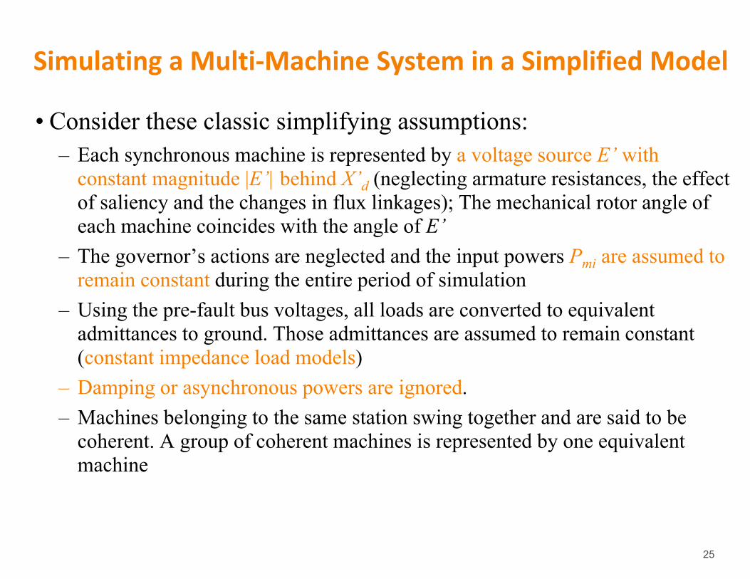
Simulating a Multi‐Machine System in a Simplified Model
• Consider these classic simplifying assumptions:– Each synchronous machine is represented by a voltage source E’ with
constant magnitude |E’| behind X’d (neglecting armature resistances, the effect of saliency and the changes in flux linkages); The mechanical rotor angle of each machine coincides with the angle of E’
– The governor’s actions are neglected and the input powers Pmi are assumed to remain constant during the entire period of simulation
– Using the pre-fault bus voltages, all loads are converted to equivalent admittances to ground. Those admittances are assumed to remain constant (constant impedance load models)
– Damping or asynchronous powers are ignored.– Machines belonging to the same station swing together and are said to be
coherent. A group of coherent machines is represented by one equivalent machine
26
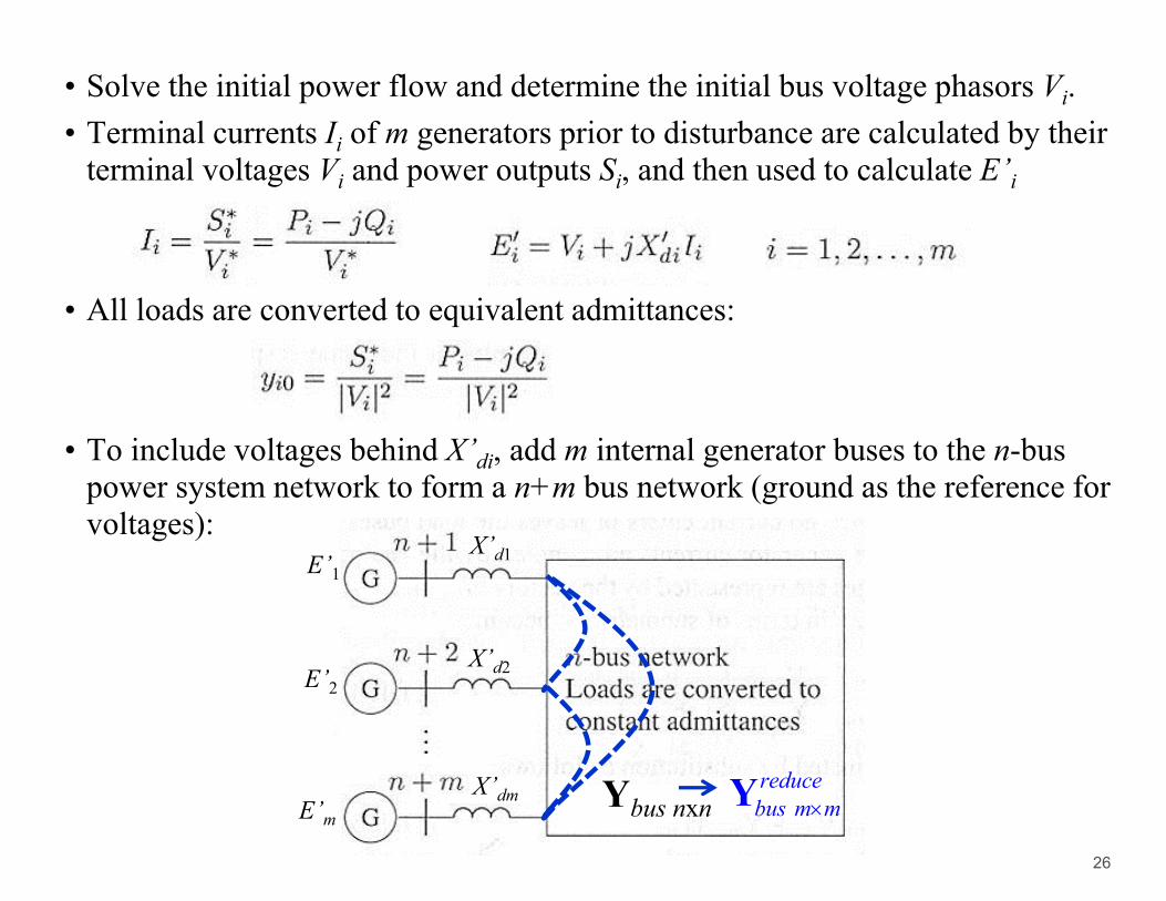
• Solve the initial power flow and determine the initial bus voltage phasors Vi. • Terminal currents Ii of m generators prior to disturbance are calculated by their
terminal voltages Vi and power outputs Si, and then used to calculate E’i
• All loads are converted to equivalent admittances:
• To include voltages behind X’di, add m internal generator buses to the n-bus power system network to form a n+m bus network (ground as the reference for voltages):
X’d1
X’d2
X’dm
E’1
E’2
E’mYbus nxn
reducebus m mY
27
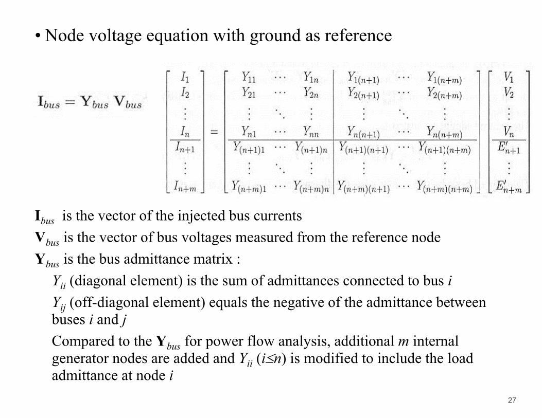
• Node voltage equation with ground as reference
Ibus is the vector of the injected bus currentsVbus is the vector of bus voltages measured from the reference nodeYbus is the bus admittance matrix :Yii (diagonal element) is the sum of admittances connected to bus iYij (off-diagonal element) equals the negative of the admittance between buses i and jCompared to the Ybus for power flow analysis, additional m internal generator nodes are added and Yii (in) is modified to include the load admittance at node i
28
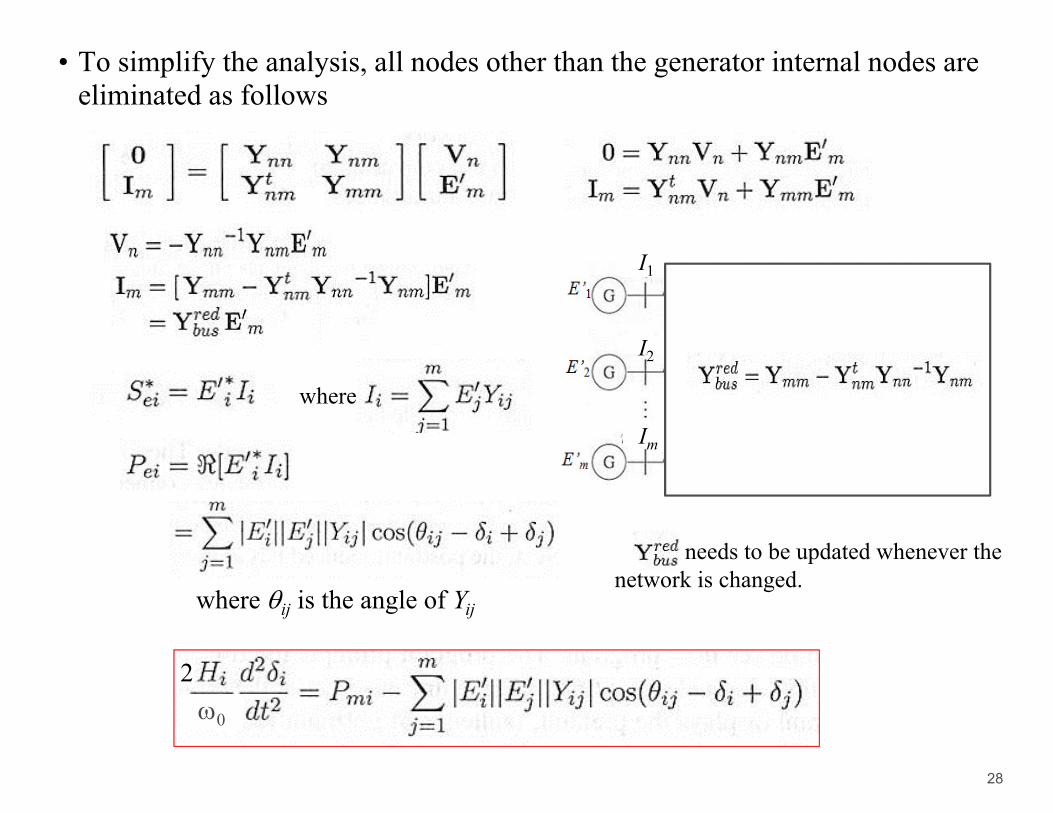
• To simplify the analysis, all nodes other than the generator internal nodes are eliminated as follows
where
where ij is the angle of Yij
I1
I2
Im
20
needs to be updated whenever the network is changed.