Embed Size (px)
Citation preview
Balázs Vajna, Erika Tóth, Tamás Felföldi
Methods in Environmental Microbiology
and Bacterial Taxonomy
Eötvös Loránd University
Department of Microbiology
Budapest, 2016
‘Supported by the Higher Education Restructuring Fund allocated to ELTE by the Hungarian Government’
2
Professional and language assistant: Károly Márialigeti
The authors would like to say special thanks to Balázs Könnyű for advices concerning
Chapter VI.
Copyright © 2016 Eötvös Loránd University
ISBN 978-963-284-806-8

3
Table of contents
List of Exercises ........................................................................................................................................... 5
List of Figures ............................................................................................................................................... 7
I. INTRODUCTION ................................................................................................................................ 9
II. CLASSICAL PHENOTYPICAL METHODS USED IN BACTERIAL TAXONOMY
(Erika Tóth) ........................................................................................................................................... 11
II.1. Morphotypes of bacteria ............................................................................................................... 11
Simple staining .................................................................................................................................... 11
Study the Gram staining preparations of pathogenic microbes by using the Gram stain-
tutorTM .................................................................................................................................................. 13
II.2. Rapid identification of bacteria - multi-test systems ................................................................ 13
III. CHEMOTAXONOMICAL METHODS USED IN BACTERIAL IDENTIFICATION
AND MICROBIAL ECOLOGY (Erika Tóth) ............................................................................... 16
III.1. The peptidoglycan structure of the cell wall of Bacteria ........................................................ 16
III.2. Study of isoprenoid quinones ..................................................................................................... 20
III.3. Study of the fatty acid profile of bacteria ................................................................................. 22
III.4. Study of the volatile fermentation end products ..................................................................... 24
III.6. Mass spectrometric methods in bacterial identification ......................................................... 25
MALDI-TOF MS (Matrix Assisted Laser Desorption/Ionization Time-Of-Flight Mass
Spectrometry) ..................................................................................................................................... 26
III.7. Community level chemotaxonomic analysis ............................................................................ 28
IV. NUCLEIC ACID BASED TECHNIQUES USED IN BACTERIAL TAXONOMY AND
MICROBIAL ECOLOGY (Balázs Vajna, Tamás Felföldi) ........................................................... 29
IV.1. Separation of nucleic acids .......................................................................................................... 29
IV.2. DNA extraction ............................................................................................................................ 36
IV.3. DNA amplification with PCR .................................................................................................... 42
Metabolic genes .................................................................................................................................. 45
IV.4. DNA sequencing .......................................................................................................................... 54
IV.5. Phylogenetic analyses ................................................................................................................... 60
IV.6. Other genotyping methods ......................................................................................................... 62
ARDRA (Amplified Ribosomal DNA Restriction Analysis) ...................................................... 62
RAPD (Random Amplification of Polymorphic DNA) .............................................................. 64
LH-PCR (Length-Heterogeneity PCR) ........................................................................................... 66
4
IV.7. Analysis of bacterial communities based on nucleic acids ..................................................... 70
DGGE (Denaturing Gradient Gel Electrophoresis) .................................................................... 70
T-RFLP (Terminal Restriction Fragment Length Polymorphism) ............................................. 74
Preparing clone libraries .................................................................................................................... 78
Microbial community analyses with NGS technologies ............................................................... 81
IV.8. Study of environmental samples in practice ............................................................................. 82
V. QUANTIFICATION OF BACTERIA (Erika Tóth) .................................................................... 84
V.1. Microscopic cell counting ............................................................................................................. 84
V.2. Quantification of different bacteria based on MPN method .................................................. 86
Quantification of hygienically relevant bacteria – study of faecal indicator organisms ........... 86
VI. DATA ANALYSIS (Balázs Vajna) ................................................................................................... 92
VI.1. Visualizing relationship among samples ................................................................................... 94
Hundred-percent stacked column chart ......................................................................................... 94
Diversity indices ................................................................................................................................. 94
Ordination ........................................................................................................................................... 95
VI.2. Identifying group of samples ...................................................................................................... 98
VI.3. Hypothesis testing ........................................................................................................................ 99
Testing the separation of groups in multivariate dataset.............................................................. 99
Testing differences among data with less dimensions ................................................................ 100
VI.4. Linking different datasets to each other ................................................................................. 102
VII. SPECIES IDENTIFICATION IN PRACTICE (Erika Tóth) ................................................ 103
Source of figures ....................................................................................................................................... 105
References ................................................................................................................................................. 106
5
List of Exercises
EXERCISE II/1.: Simple staining of bacterial strains ......................................................................... 12
EXERCISE II/2.: API test to determine biochemical activity of different bacteria ....................... 14
EXERCISE III/1.: Determination the DAP content of bacterial cells from whole cell lysate ..... 18
EXERCISE III/2.: Determination the isoprenoid quinone composition of bacterial cells ........... 20
EXERCISE III/3.: Determination the fatty acid profile of bacteria ................................................. 23
EXERCISE III/4.: Determination of the volatile fermentation end products (volatile fatty acids)
of food samples ..................................................................................................................................... 24
EXERCISE IV/1.: Agarose gel electrophoresis ................................................................................... 31
EXERCISE IV/2.: Polyacrylamide gel electrophoresis (PAGE) ....................................................... 32
EXERCISE IV/3.: Separation of DNA molecules with a model 2100 Bioanalyzer (Agilent
Technologies) ........................................................................................................................................ 33
EXERCISE IV/4.: Capillary electrophoresis of fluorescently labelled DNA .................................. 35
EXERCISE IV/5.: DNA extraction from bacterial cells with different techniques ....................... 39
EXERCISE IV/6.: DNA extraction from environmental samples with different techniques ...... 40
EXERCISE IV/7.: DNA purification with ethanol precipitation ...................................................... 41
EXERCISE IV/8.: PCR amplification of the 16S rRNA gene and its purification ........................ 44
EXERCISE IV/9.: PCR amplification of the pheU gene ..................................................................... 47
EXERCISE IV/10.: PCR amplification of the nifH gene .................................................................... 48
EXERCISE IV/11.: PCR amplification of the nodD gene .................................................................. 49
EXERCISE IV/12.: PCR amplification of the atpD gene ................................................................... 50
EXERCISE IV/13.: PCR amplification of the glnII gene .................................................................... 52
EXERCISE IV/14.: PCR amplification of the recA gene .................................................................... 53
EXERCISE IV/15.: Sanger sequencing of DNA molecules (and analysis of the obtained
chromatograms) .................................................................................................................................... 55
EXERCISE IV/16.: Phylogenetic analysis using the MEGA software ............................................. 61
EXERCISE IV/17.: Restriction digestion of PCR products and pattern analysis ........................... 63
EXERCISE IV/18.: Distinguishing bacterial strains using the RAPD fingerprinting technique .. 65
EXERCISE IV/19.: Genetic characterization of Synechococcus isolates with LH-PCR..................... 67
EXERCISE IV/20.: Grouping bacterial strains based on the length heterogeneity of the
ribosomal ITS region ............................................................................................................................ 69
EXERCISE IV/21.: DGGE analysis of environmental DNA samples ............................................ 71
EXERCISE IV/22.: T-RFLP analysis of environmental DNA samples .......................................... 75
EXERCISE IV/23.: Preparing and analysing clone libraries .............................................................. 79
EXERCISE V/1.: Enumeration of microbes with DAPI staining .................................................... 85

6
EXERCISE V/2.: Determination the total germ count of surface waters with the MPN method
................................................................................................................................................................. 86
EXERCISE V/3.: Enumeration of coliform bacteria and Escherichia coli with the Colilert system87
EXERCISE V/4.: Determination the number of enterococci with the MPN method .................. 89
EXERCISE V/5.: Determination of Clostridium perfringens from surface waters .............................. 90
7
List of Figures
Fig. II/1. Bacterial colonies on the surface of nutrient medium ......................................................... 11
Fig. II/2. Scanning electron micrograph of mycelia of Streptomyces sp. .............................................. 12
Fig. II/3. Morphological cell cycle of Aquipuribacter hungaricus ............................................................ 12
Fig. II/4. Biolog Gram-negative microplate test result after 24 hrs incubation at 37 °C ................ 14
Fig. II/5. Result of API ZYM test of different bacterial strains after 6 hours of incubation
at 37 °C ................................................................................................................................................... 15
Fig. III/1. Cell wall structure of Bacteria ................................................................................................ 16
Fig. III/2. Basic peptidoglycan structure of different bacteria ............................................................ 17
Fig. III/3. Analysis of peptidoglycan in Bacteria ................................................................................... 18
Fig. III/4. Molecular structure of quinones ........................................................................................... 20
Fig. III/5. Fatty acid profile of a novel species candidate bacterial strain, closely related to the
genus Brevundimonas ............................................................................................................................... 22
Fig. III/6. Principle of mass spectrometry ............................................................................................. 26
Fig. III/7. Basic principle of MALDI ..................................................................................................... 27
Fig. III/8. Steps of community level chemotaxonomical analysis ...................................................... 28
Fig. IV/1. DNA markers used for gel electrophoresis ......................................................................... 30
Fig. IV/2. The Agilent 2100 Bioanalyzer on-chip electrophoresis system ........................................ 34
Fig. IV/3. ABI PrismTM 310 Genetic Analyser ...................................................................................... 36
Fig. IV/4. Mixer mill (model MM301, Retsch) ...................................................................................... 37
Fig. IV/5. Amplification of a DNA fragment with Polymerase Chain Reaction (PCR) ................. 43
Fig. IV/6. Regions of the 16S rRNA gene and binding sites of selected universal primers ........... 43
Fig. IV/7. DNA sequence determination based on the Sanger method ........................................... 55
Fig. IV/8. A chromatogram generated after Sanger sequencing of DNA......................................... 55
Fig. IV/9. The Ion Torrent PGMTM (Life Technologies) next-generation DNA sequencing system
................................................................................................................................................................. 58
Fig. IV/10. The GS Junior (Roche) next-generation DNA sequencing system ............................... 59
Fig. IV/11. Picotiter plate and semiconductor chip used for next-generation DNA sequencing . 59
Fig. IV/12. A pyrosequencing flowgram generated on a Roche GS Junior system ......................... 60
Fig. IV/13. Amplified Ribosomal DNA Restriction Analysis (ARDRA) pattern of PCR products
................................................................................................................................................................. 62
Fig. IV/14. Clustering of strains with the RAPD fingerprinting technique. ..................................... 64
Fig. IV/15. Position of genes encoding phycobilisome proteins ........................................................ 66
Fig. IV/16. Outline of the DGGE technique ........................................................................................ 71
8
Fig. IV/17. Result of DGGE analysis of environmental DNA samples based on the partial
16S rRNA gene...................................................................................................................................... 74
Fig. IV/18. Outline of the T-RFLP technique ...................................................................................... 75
Fig. IV/19. T-RFLP electropherogram of environmental DNA samples based on the partial
16S rRNA gene...................................................................................................................................... 78
Fig. IV/20. Outline of preparing and analysing clone libraries ........................................................... 79
Fig. IV/21. Methods in the analysis of microbial community structure ............................................ 82
Fig. IV/22. General process workflow of T-RFLP-, DGGE- and cloning and sequencing-based
environmental microbiological studies .............................................................................................. 83
Fig. V/1. Epifluorescence microscopic image of DAPI stained cells from a water sample ........... 84
Fig. V/2. Detection of coliform and E. coli in Quanti-Tray bags ....................................................... 88
Fig. V/3. Enumeration of C. perfringens on the surface of TSC medium ........................................... 91
Fig. VI/1. Part of our example T-RFLP data matrix ............................................................................ 92
Fig. VI/2. Hundred-percent stacked column chart of our example T-RFLP dataset ..................... 94
Fig. VI/3. Simpson and Shannon indices of the samples based on our example T-RFLP dataset
................................................................................................................................................................. 95
Fig. VI/4. Principal component analysis (PCA) of our example T-RFLP dataset ........................... 96
Fig. VI/5. Non-metric multidimensional scaling (NMDS) based on Bray-Curtis distances of our
example T-RFLP dataset ..................................................................................................................... 97
Fig. VI/6. Dendrogram resulting from Bray-Curtis distances based UPGMA cluster analysis of
our example T-RFLP dataset .............................................................................................................. 98
Fig. VI/7. Bray-Curtis distances among samples in our example dataset .......................................... 99
Fig. VI/8. Physicochemical parameters of the Stage 7 samples in our example dataset ............... 100
Fig. VI/9. Shannon index of samples in our example dataset grouped according to stages ........ 101
Fig. VI/10. Analysing linear correlations among physicochemical variables in our example dataset
............................................................................................................................................................... 101
Fig. VI/11. Comparing T-RFLP fingerprints and diversity indices in our example dataset ......... 102
Fig. VII/1. Basic steps of description of novel taxa ........................................................................... 104
9
I. INTRODUCTION
Methods applied for the analysis of bacterial strains and also those applied for the study of
microbial communities inhabiting different environments have been changed significantly in the
last decades, and therefore some of these methods were not introduced in many of general
microbiological laboratories. Nevertheless, basic techniques used for the determination of general
physiological properties (e.g. cell and colony morphology; basic cell wall structure; temperature,
pH and salt tolerance of individual bacterial strains or their carbon source utilization and
antibiotics resistance profile) are still in use and play an important role in several fields of
microbiology (e.g. in the description of new taxa or in clinical microbiology). The most important
ones among these techniques have been incorporated in our recent practical entitled ‘Practical
Microbiology’ (2013, Edited by: E.M. Tóth and K. Márialigeti). The purpose of that guide was to
give a collection of exercises covering the most important fields of general microbiology, and to
introduce the students into the work in a microbiological laboratory, to acquire the skills needed
for aseptic work, to learn how to handle living cultures and to get familiar with the general
techniques of microbiology. Therefore, the major aim to compile this practical was to give a
collection of such a set of methods, which are applied currently in bacterial taxonomic analyses
(e.g. description of new species and genera or revision of existing taxa) and those applied for the
study of microbial communities in various environments.
At first sight, the two above mentioned fields (taxonomy and environmental microbiology) may
be unrelated and gathering exercises related to these areas of microbiology may look constrained,
although, the basis of many of environmental investigations is the correct identification of
bacterial/microbial taxa, which serves as a link between taxonomy and environmental
microbiology. Furthermore, many techniques suitable for the study of individual strains can be
applied (with some modification and supplementation) also for the analysis of complex microbial
communities. Therefore, in this practical book, we provide an overview of the procedures used in
environmental microbiological studies and in bacterial taxonomy. Although this collection of
methods is not exhaustive, most common classical phenotypic, chemotaxonomic and nucleic
acid-based techniques, methods applied for the enumeration of bacteria and a survey of data
analysis are presented here with a short note on the integration of these methods in the
microbiological study of environmental samples and in bacterial taxonomy.
The Authors

10
Please consult Chapter 2 of ‘Practical Microbiology’ (2013, Edited by: E.M. Tóth and K. Márialigeti) for the
safety regulations that should be applied during the work in a microbiological laboratory.
11
II. CLASSICAL PHENOTYPICAL METHODS USED
IN BACTERIAL TAXONOMY (Erika Tóth)
II.1. Morphotypes of bacteria
The morphological characteristics of bacteria have diagnostic value.
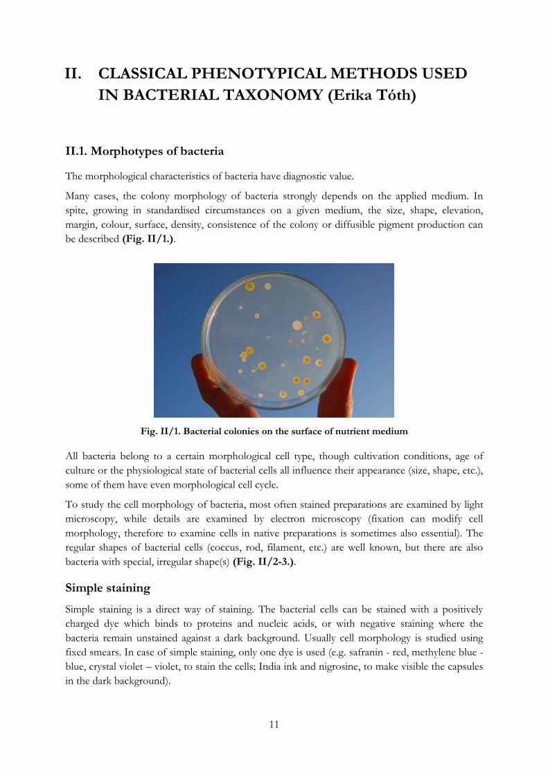
Many cases, the colony morphology of bacteria strongly depends on the applied medium. In
spite, growing in standardised circumstances on a given medium, the size, shape, elevation,
margin, colour, surface, density, consistence of the colony or diffusible pigment production can
be described (Fig. II/1.).
Fig. II/1. Bacterial colonies on the surface of nutrient medium
All bacteria belong to a certain morphological cell type, though cultivation conditions, age of
culture or the physiological state of bacterial cells all influence their appearance (size, shape, etc.),
some of them have even morphological cell cycle.
To study the cell morphology of bacteria, most often stained preparations are examined by light
microscopy, while details are examined by electron microscopy (fixation can modify cell
morphology, therefore to examine cells in native preparations is sometimes also essential). The
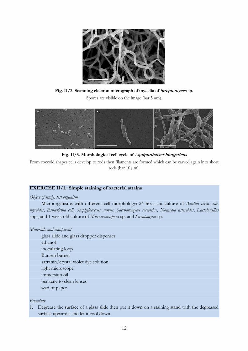
regular shapes of bacterial cells (coccus, rod, filament, etc.) are well known, but there are also
bacteria with special, irregular shape(s) (Fig. II/2-3.).
Simple staining
Simple staining is a direct way of staining. The bacterial cells can be stained with a positively
charged dye which binds to proteins and nucleic acids, or with negative staining where the
bacteria remain unstained against a dark background. Usually cell morphology is studied using
fixed smears. In case of simple staining, only one dye is used (e.g. safranin - red, methylene blue -
blue, crystal violet – violet, to stain the cells; India ink and nigrosine, to make visible the capsules
in the dark background).
12
Fig. II/2. Scanning electron micrograph of mycelia of Streptomyces sp.
Spores are visible on the image (bar 5 µm).
Fig. II/3. Morphological cell cycle of Aquipuribacter hungaricus
From coccoid shapes cells develop to rods then filaments are formed which can be carved again into short
rods (bar 10 µm).
EXERCISE II/1.: Simple staining of bacterial strains
Object of study, test organism
Microorganisms with different cell morphology: 24 hrs slant culture of Bacillus cereus var.
mycoides, Eshcerichia coli, Staphylococcus aureus, Saccharomyces cerevisiae, Nocardia asteroides, Lactobacillus
spp., and 1 week old culture of Micromomospora sp. and Streptomyces sp.
Materials and equipment
glass slide and glass dropper dispenser
ethanol
inoculating loop
Bunsen burner
safranin/crystal violet dye solution
light microscope
immersion oil
benzene to clean lenses
wad of paper
Procedure
1. Degrease the surface of a glass slide then put it down on a staining stand with the degreased
surface upwards, and let it cool down.
13
2. When it is cooled, label the degreased slide adequately.
3. Put a small drop of water onto the slide, then suspend a small loopful of bacterial culture in
it. Thereafter make a film layer (smear) with the needle of the inoculating loop and let it dry.
4. Fix your preparation with heat over the Bunsen burner: move the slide over the flame
carefully 2-4 times, do not warm it up strongly.
5. Drop safranin/crystal violet dye onto the fixed smear until it is fully covered and stain for 1
minute.
6. Wash the smear with tap water to remove excess dye solution.
7. Dry the slide.
8. During microscopy, first use 40×, then 100× objective lenses. In the latter case, use
immersion oil.
9. Observe the morphology of the cells and draw the microscopic picture to be able to identify
the bacterium after given standard preparations.
10. After finishing microscopic observation, clean all used objective lenses with benzene (do not
use ethanol for this purpose as it can dissolve lens adhesives).
Study the Gram staining preparations of pathogenic microbes by using the
Gram stain-tutorTM
Gram staining preparations can be studied in tutor software, e.g. by Gram stain-tutorTM. This
software is adequate to check the morphology and possible staining characteristics of pathogenic
bacteria. The software presents Gram staining micrographs of different microbes, including pure
cultures and also that of complex samples (e.g. human/animal tissues).
II.2. Rapid identification of bacteria - multi-test systems
Many rapid multi-test systems for identifying bacteria are available nowadays (Table II/1.).
These systems offer the advantages of miniaturization and are usually used in connection with a
computerized setup for the identification of (micro)organisms. Most are based on the
biochemical reactions of strains. It is important to know that these systems are designed for the
identification of particular taxa though multi-test systems can provide useful information on the
physiological characteristics of microorganisms. The reactions may not always agree with the
results from classical characterization tests or with the results obtained with other multi-test
systems. Using multitest systems care should be taken to adhere to the instructions (e.g. inoculum
age and size, incubation temperature) to retain adequate results.
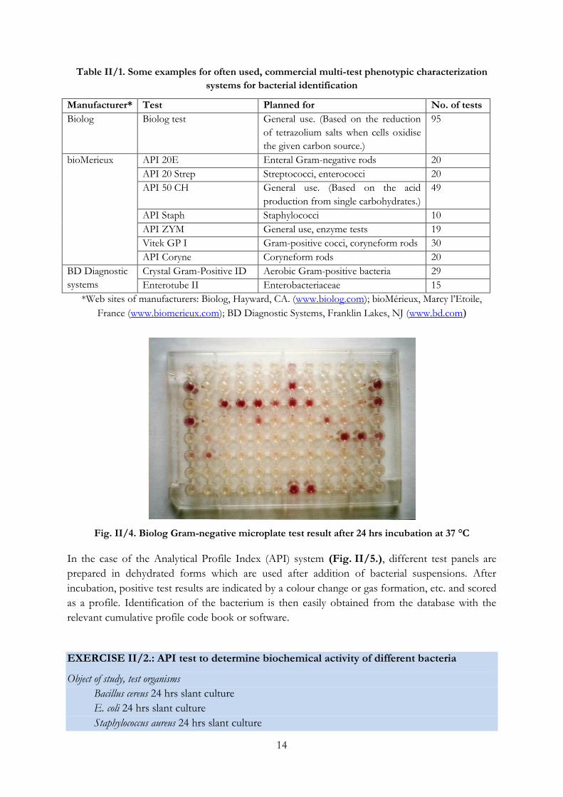
The BIOLOG rapid identification system (Fig. II/4.) is based on the utilization of 95 different
carbon sources, which could be used as sole source of carbon or energy for the tested
microorganism. The result of the test is a kind of metabolic fingerprint of the given bacterium.
The microtiter plates contain the carbon sources, a buffer, and also a redox dye (tetrazolium) in
lyophilized form: when a compound is utilized, the redox dye is reduced and turns from
colourless into violet colour (formazan) indicating the oxidation of the carbon source. The
system can be connected to a microplate reader and computer database and analysis software.
Based on its oxidation pattern the unknown bacterium strain can be identified.
14
Table II/1. Some examples for often used, commercial multi-test phenotypic characterization
systems for bacterial identification
Manufacturer* Test Planned for No. of tests
Biolog Biolog test General use. (Based on the reduction
of tetrazolium salts when cells oxidise
the given carbon source.)
95
bioMerieux API 20E Enteral Gram-negative rods 20
API 20 Strep Streptococci, enterococci 20
API 50 CH General use. (Based on the acid
production from single carbohydrates.)
49
API Staph Staphylococci 10
API ZYM General use, enzyme tests 19
Vitek GP I Gram-positive cocci, coryneform rods 30
API Coryne Coryneform rods 20
BD Diagnostic
systems
Crystal Gram-Positive ID Aerobic Gram-positive bacteria 29
Enterotube II Enterobacteriaceae 15
*Web sites of manufacturers: Biolog, Hayward, CA. (www.biolog.com); bioMérieux, Marcy l’Etoile,
France (www.biomerieux.com); BD Diagnostic Systems, Franklin Lakes, NJ (www.bd.com)
Fig. II/4. Biolog Gram-negative microplate test result after 24 hrs incubation at 37 °C
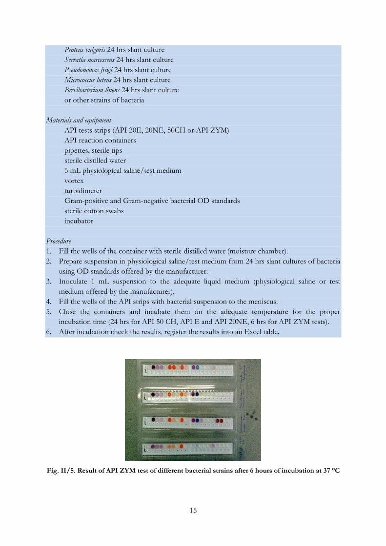
In the case of the Analytical Profile Index (API) system (Fig. II/5.), different test panels are
prepared in dehydrated forms which are used after addition of bacterial suspensions. After
incubation, positive test results are indicated by a colour change or gas formation, etc. and scored
as a profile. Identification of the bacterium is then easily obtained from the database with the
relevant cumulative profile code book or software.
EXERCISE II/2.: API test to determine biochemical activity of different bacteria
Object of study, test organisms
Bacillus cereus 24 hrs slant culture
E. coli 24 hrs slant culture
Staphylococcus aureus 24 hrs slant culture
15
Proteus vulgaris 24 hrs slant culture
Serratia marcescens 24 hrs slant culture
Pseudomonas fragi 24 hrs slant culture
Micrococcus luteus 24 hrs slant culture
Brevibacterium linens 24 hrs slant culture
or other strains of bacteria
Materials and equipment
API tests strips (API 20E, 20NE, 50CH or API ZYM)
API reaction containers
pipettes, sterile tips
sterile distilled water
5 mL physiological saline/test medium
vortex
turbidimeter
Gram-positive and Gram-negative bacterial OD standards
sterile cotton swabs
incubator
Procedure
1. Fill the wells of the container with sterile distilled water (moisture chamber).
2. Prepare suspension in physiological saline/test medium from 24 hrs slant cultures of bacteria
using OD standards offered by the manufacturer.
3. Inoculate 1 mL suspension to the adequate liquid medium (physiological saline or test
medium offered by the manufacturer).
4. Fill the wells of the API strips with bacterial suspension to the meniscus.
5. Close the containers and incubate them on the adequate temperature for the proper
incubation time (24 hrs for API 50 CH, API E and API 20NE, 6 hrs for API ZYM tests).
6. After incubation check the results, register the results into an Excel table.
Fig. II/5. Result of API ZYM test of different bacterial strains after 6 hours of incubation at 37 °C
16
III. CHEMOTAXONOMICAL METHODS USED IN
BACTERIAL IDENTIFICATION AND
MICROBIAL ECOLOGY (Erika Tóth)
Chemotaxonomy in general is a method in taxonomy based on similarities/differences in the
composition of certain compounds among the organisms, based on the analysis of chemical
markers of the cell. Chemical data often can be used to define relationships at all levels of the
taxonomic hierarchy (qualitative and quantitative analysis). It is possible to view all systematics as
‘chemosystematics’ since morphological characters, pigmentation, serology or the biochemical
properties of organisms reflect their chemical composition.
These studied markers show discontinuous distribution among different taxonomic ranks. They
must be characters which are more or less independent from cultivation conditions. At the same
time there must exist a practical, simple method for isolation and characterisation of these marker
molecules. In case of microorganisms the main chemotaxonomical biomarkers are present in the
cell wall (peptidoglycan and derivatives, teichoic acids and derivatives, mycolic acids in many
Gram-positive bacteria, etc.) and in the cytoplasmic membrane (lipid soluble pigments,
isoprenoid quinones, polar lipids, fatty acids, etc.). Chemotaxonomy also deals with techniques
yielding fingerprints or signatures of whole organisms (pyrolysis gas chromatography, mass
spectrometry, infrared spectrometry, Raman spectroscopy, etc.).
III.1. The peptidoglycan structure of the cell wall of Bacteria
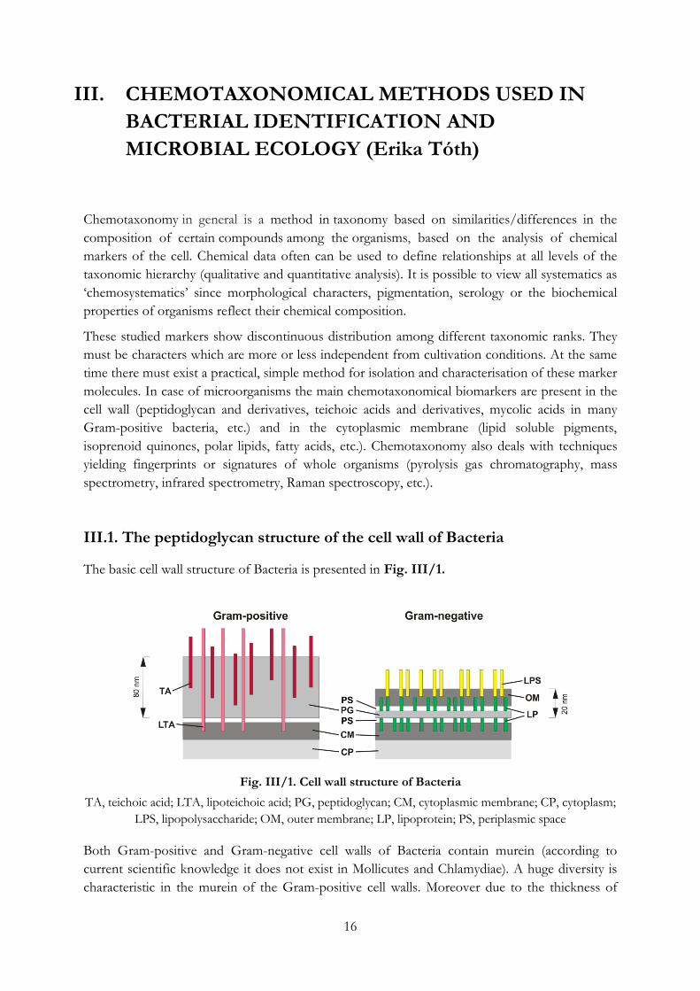
The basic cell wall structure of Bacteria is presented in Fig. III/1.
Fig. III/1. Cell wall structure of Bacteria
TA, teichoic acid; LTA, lipoteichoic acid; PG, peptidoglycan; CM, cytoplasmic membrane; CP, cytoplasm;
LPS, lipopolysaccharide; OM, outer membrane; LP, lipoprotein; PS, periplasmic space
Both Gram-positive and Gram-negative cell walls of Bacteria contain murein (according to
current scientific knowledge it does not exist in Mollicutes and Chlamydiae). A huge diversity is
characteristic in the murein of the Gram-positive cell walls. Moreover due to the thickness of

17
peptidoglycan layer, the whole wall of Gram-positive cells can be isolated and analysed relatively
easily. Peptidoglycan constitutes between 40-80% of the wall weight, it is a covalently linked net
structure, the remainder is made up of other covalently-bound macromolecules.
Peptidoglycan has a constant amino sugar backbone (as depicted below) and amino acid side
chain (Fig III/2.). These oligopeptides of the peptidoglycan can be connected to one another
and can form a net-like structure, called as murein. The most important and variable
characteristic in cell wall structure is the composition of connecting oligopeptides and the
structure of interpeptide bridges within the murein layer.
Fig. III/2. Basic peptidoglycan structure of different bacteria
NAM (N-acetylmuramic acid), NAG (N-acetylglucosamine), DAP (Diaminopimelic acid)
Different taxonomic ranks can be characterised based on that: if the diaminoacid of the cell wall
of two bacteria differs, they cannot belong even to the same genus.
There are two basic types of peptidoglycan.
Peptidoglycan A-type:
In the 3rd position of the amino acid side chain, the diamino acid binds to a D-alanine in the 4th
position of another oligopeptide chain: directly or through a bridge peptide. If there is an
interpeptide bridge, it can show also characteristic variations.
Peptidoglycan B-type:
A D-glutamic acid of the oligopeptide in the 2nd position binds to a D-alanine of the other
oligopeptide in 4th position through an interpeptide bridge.
During the characterisation of the cell wall of a given taxon the following questions are raised:
18
Which diamino acid is present in the cell wall (TLC – thin layer chromatography
determination)?
Which other amino acids are present (TLC determination)?
What is the quantitative ratio of amino acids (GC-MS determination)?
Which enantiomers exist in the peptide chains (derivatisation - N-pentafluoropropionyl
amino acid isopropyl esters, then GC determination)?
What is the sequence of amino acids (determination of N-terminal amino acid)?
Glycolyl or acetyl group on muramic acid occur in the molecule (colorimetric
determination)?
Which diagnostic sugars exist in the cell wall (TLC determination)?
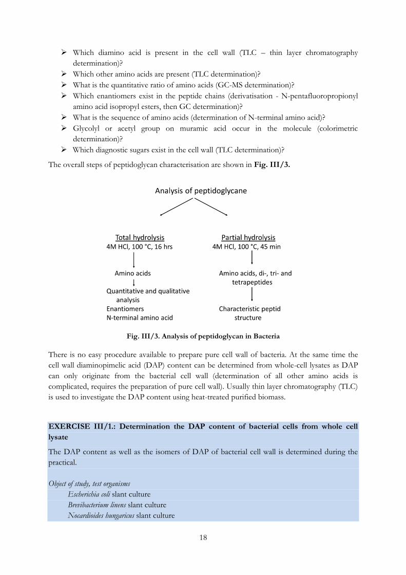
The overall steps of peptidoglycan characterisation are shown in Fig. III/3.
Fig. III/3. Analysis of peptidoglycan in Bacteria
There is no easy procedure available to prepare pure cell wall of bacteria. At the same time the
cell wall diaminopimelic acid (DAP) content can be determined from whole-cell lysates as DAP
can only originate from the bacterial cell wall (determination of all other amino acids is
complicated, requires the preparation of pure cell wall). Usually thin layer chromatography (TLC)
is used to investigate the DAP content using heat-treated purified biomass.
EXERCISE III/1.: Determination the DAP content of bacterial cells from whole cell
lysate
The DAP content as well as the isomers of DAP of bacterial cell wall is determined during the
practical.
Object of study, test organisms
Escherichia coli slant culture
Brevibacterium linens slant culture
Nocardioides hungaricus slant culture
19
Tsukamurella paurometabolum slant culture
Arthrobacter variabilis slant culture
Bacillus cereus slant culture
Nocardioides sp. slant culture
Pseudomonas fragi slant culture
or other strains of bacteria
Materials and equipment
4 mL glass screw capped sample tubes with Teflon-lined screw cap
containing 300 L 6 M HCl solution
dry block thermostat with thermometer
laboratory oven
activated carbon powder
pipette, pipette tips, filter paper
cellulose TLC plate
glass developing tank for running TLC
solvents (methanol, distilled water, 6 M HCl solution, pyridine)
DAP standard solution (0.01 g/mL)
ninhydrin reagent (0.2 w/v% solution in butanol)
Procedure
1. Place 10 loopful of bacteria into a glass sample tube containing 6 M HCl solution, and close it
tightly with the Teflon-lined screw cap.
2. For the destruction of cells (and cell walls), incubate it at 121 °C for 20 min in a dry block
thermostat.
3. Spill the content into a watch glass and evaporate the remaining HCl at 70 °C in a laboratory
oven.
4. Add 100-150 L distilled water and dissolve the brownish precipitate.
5. To purify the precipitate, prepare a filter from a 1 mL pipette tip (using filter paper and
activated carbon powder) and then filter the lysate through this filter tip.
6. Prepare the TLC plate by marking the starting line with a soft pencil, apply 8 μL lysate using
a small pipette tip and hairdryer to get as small spots as possible. As standard, use 1% DAP
solution (positive control).
7. Run TLC plates (using methanol : distilled water : 6 M HCl : pyridine in 80:26:4:10 ratio as
solvent mixture) for 2-2.5 hours in a cooled room or in a refrigerator (at 4-10 °C). (To
prepare solvent mixture use rubber gloves!)
8. For the visualisation of the chromatogram, spray it with ninhydrin reagent, and incubate the
plates in an oven at 100 °C for 5 minutes. DAP forms greyish-coloured spots.
9. Evaluate the results, compare the DAP content of different bacterial strains. The
stereoisomers of DAP will be separated, their retention factors differ strongly.
20
III.2. Study of isoprenoid quinones
Isoprenoid quinones are found in the vast majority of the aerobic or anaerobic respiring
organisms and are located in their cytoplasmic membrane as mobile proton and electron carriers
of their electron transport chains. In bacteria the two most important quinone groups are the
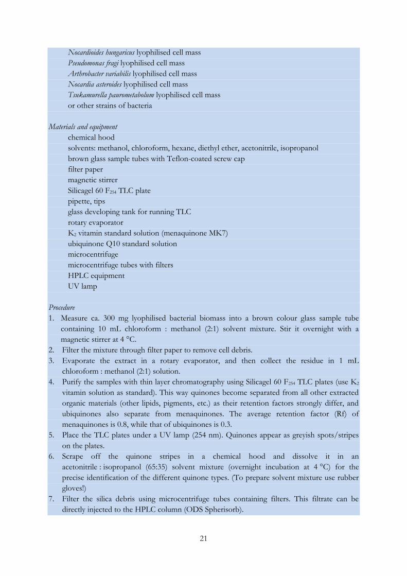
ubiquinones and menaquinones. Based on their chemical structures, ubiquinones are 2,3-
dimethoxy-5-methyl-1,4-benzoquinone molecules or its derivatives while menaquinones have 2-
methyl-3-phytyl-1,4-naphthoquinone type structures (Fig. III/4.).
The respiratory quinones have great taxonomic significance as the type of quinone present in an
organism and the isoprenoid chain length often reflect the phylogenetic affiliation of a given
bacterial taxon. Ubiquinones are widespread in nature, occur in plants, animals and many
microbes, among them in most Gram-negative bacteria but never occur in Gram-positives or
Archaea. Menaquinones are present both in Bacteria and Archaea: wholly unsaturated forms
occur in Bacteria with peptidoglycan B-type and low G+C Gram-positives; partially saturated
menaquinones occur in high G+C Bacteria (Actinobacteria) and bacteria with A-type
peptidoglycan and also in some Gram-negative bacteria; completely saturated menaquinones
appear only in Archaea (e.g. in Pyrobaculum islandicum). Cyclic menaquinones are genus-specific
markers of genera Nocardia and Skermania.
Most organisms produce mixtures of either menaquinones or ubiquinones with different
polyprenyl lengths, though one is generally the major respiratory quinone. When facultative
anaerobic Gram-negative bacteria change their respiration to anaerobic from aerobic, they change
also their quinone profile (e.g. Escherichia coli produces primarily ubiquinone-8 under aerobic
condition, but menaquinone-8 is produced when it grows anaerobically on nitrate).
(a) (b)
Fig. III/4. Molecular structure of quinones
(a) ubiquinone, (b) unsaturated menaquinone, ‘n’ is the number of isoprenoid units within the side chain
Isoprenoid quinones are sensitive molecules, can be easily degraded, so all extraction steps must
be performed in protection from light, preferably in brown glass tubes to prevent photo-
oxidation, and if possible under N2 atmosphere.
EXERCISE III/2.: Determination the isoprenoid quinone composition of bacterial cells
Object of study, test organisms
Escherichia coli lyophilised cell mass
Brevibacterium linens lyophilised cell mass
21
Nocardioides hungaricus lyophilised cell mass
Pseudomonas fragi lyophilised cell mass
Arthrobacter variabilis lyophilised cell mass
Nocardia asteroides lyophilised cell mass
Tsukamurella paurometabolum lyophilised cell mass
or other strains of bacteria
Materials and equipment
chemical hood
solvents: methanol, chloroform, hexane, diethyl ether, acetonitrile, isopropanol
brown glass sample tubes with Teflon-coated screw cap
filter paper
magnetic stirrer
Silicagel 60 F254 TLC plate
pipette, tips
glass developing tank for running TLC
rotary evaporator
K2 vitamin standard solution (menaquinone MK7)
ubiquinone Q10 standard solution
microcentrifuge
microcentrifuge tubes with filters
HPLC equipment
UV lamp
Procedure
1. Measure ca. 300 mg lyophilised bacterial biomass into a brown colour glass sample tube
containing 10 mL chloroform : methanol (2:1) solvent mixture. Stir it overnight with a
magnetic stirrer at 4 °C.
2. Filter the mixture through filter paper to remove cell debris.
3. Evaporate the extract in a rotary evaporator, and then collect the residue in 1 mL
chloroform : methanol (2:1) solution.
4. Purify the samples with thin layer chromatography using Silicagel 60 F254 TLC plates (use K2
vitamin solution as standard). This way quinones become separated from all other extracted
organic materials (other lipids, pigments, etc.) as their retention factors strongly differ, and
ubiquinones also separate from menaquinones. The average retention factor (Rf) of
menaquinones is 0.8, while that of ubiquinones is 0.3.
5. Place the TLC plates under a UV lamp (254 nm). Quinones appear as greyish spots/stripes
on the plates.
6. Scrape off the quinone stripes in a chemical hood and dissolve it in an
acetonitrile : isopropanol (65:35) solvent mixture (overnight incubation at 4 °C) for the
precise identification of the different quinone types. (To prepare solvent mixture use rubber
gloves!)
7. Filter the silica debris using microcentrifuge tubes containing filters. This filtrate can be
directly injected to the HPLC column (ODS Spherisorb).
22
8. Use the chromatograms of other authentic strains and standard Q10 as well as MK7 solution
for data evaluation. There is a linear correlation between the logarithm of retention times and
the number of isoprenoid units in the quinone side chain. This helps to identify the peaks on
the chromatograms.
9. Evaluate your data on a semi-logarithmic paper (or with use of Microsoft Excel) and
compare the quinone profiles of the different bacterial strains.
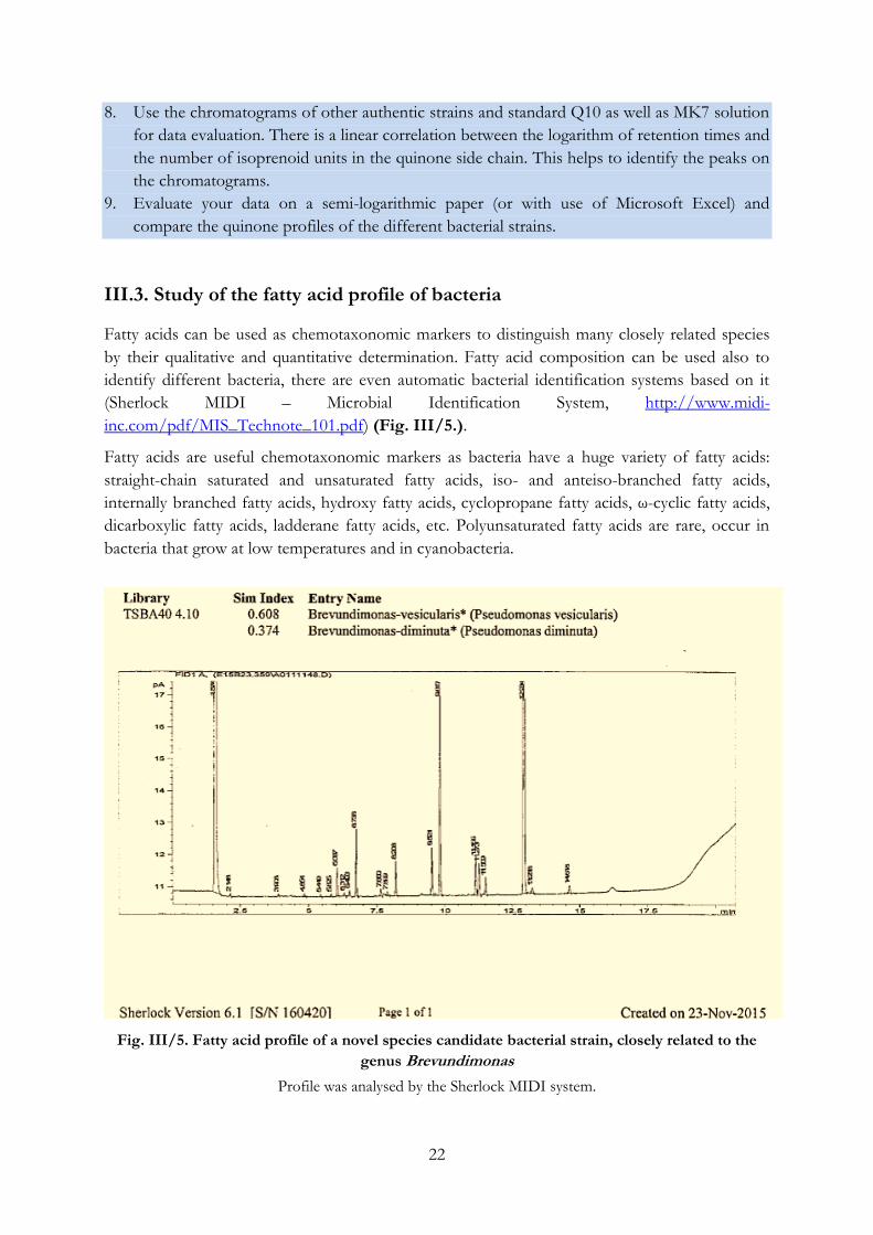
III.3. Study of the fatty acid profile of bacteria
Fatty acids can be used as chemotaxonomic markers to distinguish many closely related species
by their qualitative and quantitative determination. Fatty acid composition can be used also to
identify different bacteria, there are even automatic bacterial identification systems based on it
(Sherlock MIDI – Microbial Identification System, http://www.midi-
inc.com/pdf/MIS_Technote_101.pdf) (Fig. III/5.).
Fatty acids are useful chemotaxonomic markers as bacteria have a huge variety of fatty acids:
straight-chain saturated and unsaturated fatty acids, iso- and anteiso-branched fatty acids,
internally branched fatty acids, hydroxy fatty acids, cyclopropane fatty acids, ω-cyclic fatty acids,
dicarboxylic fatty acids, ladderane fatty acids, etc. Polyunsaturated fatty acids are rare, occur in
bacteria that grow at low temperatures and in cyanobacteria.
Fig. III/5. Fatty acid profile of a novel species candidate bacterial strain, closely related to the
genus Brevundimonas
Profile was analysed by the Sherlock MIDI system.
23
The most important factor to obtain reproducible and comparable fatty acid composition of
different bacteria is to standardize the growth conditions of the organisms being examined, since
the levels of the different fatty acids vary with the growth temperature, the phase of growth and
the medium composition, etc.
Obtaining pure fatty acids contains four steps: after standardised cultivation wet bacterial
biomass used directly for saponification (liberation of fatty acids from fats and oils), esterification
(to form fatty acid methyl esters), extraction (of fatty acid methyl esters with solvents) and
purification of the extract (washing step).
Fatty acid composition is revealed by gas chromatography (GC) at the end and by comparison of
the peak retention times of samples with those of known standards (BAME: Bacterial Methyl
Ester). If a peak remains still unidentified, mass spectrometry can be used (GC-MS). The use of
Sherlock Microbial Identification Systems (MIDI) (www.midi-inc.com) is common, as this system
provides a highly standardized methodology.
EXERCISE III/3.: Determination the fatty acid profile of bacteria
Object of study, test organisms
Log-phase cultures (usually 24 hours) grown on TSA medium at 28 °C:
Escherichia coli
Brevibacterium linens
Nocardioides hungaricus
Pseudomonas fragi
Arthrobacter variabilis
or other strains of bacteria
Materials and equipment
10 mL glass sample tubes with Teflon-lined screw caps
Reagent 1 - for saponification (NaOH, methanol, distilled water),
Reagent 2 - for methylation (6 M HCl, methanol)
Reagent 3 – for extraction (hexane, tert-methyl-buthyl-ether)
Reagent 4 – for base wash (NaOH, distilled water)
vortex mixer
overhead mixer
degreased glass tubes
water bath
slush ice
degreased Pasteur pipettes
1 mL glass tubes for sample storage
microliter syringe
gas chromatograph (GC)
BAME (Bacterial Methyl Ester) standard solution
24
Procedure
1. Add 1 mL Reagent 1 to 2-3 loopful of bacteria in glass sample tubes, close with Teflon-lined
screw caps.
2. Vortex and incubate at 100 °C in a water bath for 5 minutes (saponification).
3. Vortex again and put the tubes back to the 100 °C water bath for 25 min, then cool them
down suddenly in slush ice.
4. Add 2 mL Reagent 2 and vortex.
5. Incubate it in 80 °C water bath for 10 minutes, then cool them suddenly in slush ice.
6. After this methylation process, add 1.25 mL Reagent 3 and mix with overhead mixer for 10
minutes.
7. Discard the lower phase using Pasteur pipette and add 3 mL Reagent 4 to the upper, ‘solvent’
phase, mix for 5 minutes. Storage of these fatty acid samples is possible in 1 mL sample
tubes at -20 °C for a few weeks.
8. 1 L from this liquid can be directly injected into a gas chromatograph. [(Conditions of GC
analysis: splitless injection, capillary column (SPB-1, 30 × 32 mm id.), FID detector, 280 °C.)]
Evaluate the data with the help of BAME (Bacterial Methyl Ester) standard and compare the
results of different bacteria.
III.4. Study of the volatile fermentation end products
Short chain fatty acids are the most important intermediates or end-products of different
fermentation processes. Fermentation pathways can be mapped with the study of these
molecules. Such analyses have importance in the food industry and support also the classification
of anaerobic, fermentative bacteria. The different types of fermentations are characteristic to a
given taxon.
EXERCISE III/4.: Determination of the volatile fermentation end products (volatile fatty
acids) of food samples
Object of study, test organisms
various cheeses and other dairy products (e.g. yoghurt)
Materials and equipment
microcentrifuge with tubes
vortex mixer
freezer
50% H2SO4 solution
methyl-t-butyl-ether (MTBE)
CaCl2 crystals
microliter syringe
standard solution (formic acid, acetic acid, propionic acid, isobutyric acid, butyric acid,
valeric acid, isovaleric acid; Table III/1.)
gas chromatograph
25
Procedure
1. Pipette 1-2 g homogenised food product (cheese/yoghurt) into a microcentrifuge tube, and
then add 0.05 mL 50% H2SO4 and 0.5 mL methyl-t-butyl-ether solution.
2. Vortex for 5-10 sec.
3. Centrifuge the mixture to break the emulsion.
4. Transfer the upper phase (ether-phase) to a clean microcentrifuge tube, then put it into the
freezer (-20 °C) to freeze the remaining water.
5. Rapidly transfer the liquid phase to a clean microcentrifuge tube and put CaCl2 crystals into
the tube to extract all residual water.
6. Inject 1 L to a GC from each sample and also from the control solution and determine the
volatile acid-composition (GC parameters are given in Table III/1.).
7. Evaluate your data and compare the volatile compounds of different food products.
Table III/1. Chromatography parameters during VFA (volatile fatty acid) determination
Chromatography Standard
(in 100 mL distilled water)
Column type 19001c-003
6 ft 10% FFAP
1% H3PO4
formic acid (50%) 0.114 mL
acetic acid (96%) 0.037 mL
propionic acid 0.075 mL
Detector type FID (Flame ionisation detector) isobutyric acid 0.092 mL
Column temp. 145 °C butyric acid 0.091 mL
Injector temp. 180 °C valeric acid 0.109 mL
Detector temp. 190 °C isovaleric acid 0.109 mL
III.6. Mass spectrometric methods in bacterial identification
Mass spectrometry is the branch of analytical chemistry which runs on the determination of the
mass of charged particles. It can be applied for the direct study of organic compounds or can be
connected to different separation techniques (e.g. GC-MS, LC-MS). The charged particles are
arisen in the ion source then in the mass-analyser they are transferred via an electromagnetic field
meanwhile they are separated based on their mass/charge. Ions are detected and from the
detected signal a mass spectrum is generated.
Ionisation can be reached on different ways. To study biological material, usually soft ionisation
methods are used which do not fragment the studied molecule (e.g. Electrospray Ionisation –
ESI; Matrix Assisted Laser Desorption Ionization – MALDI).
Characteristics and steps of mass spectrometry analysis:
Sample transfer to gas phase
Ionization of gas-phase particles
Separation in an electromagnetic field by m/z (mass/charge)
Detection
26
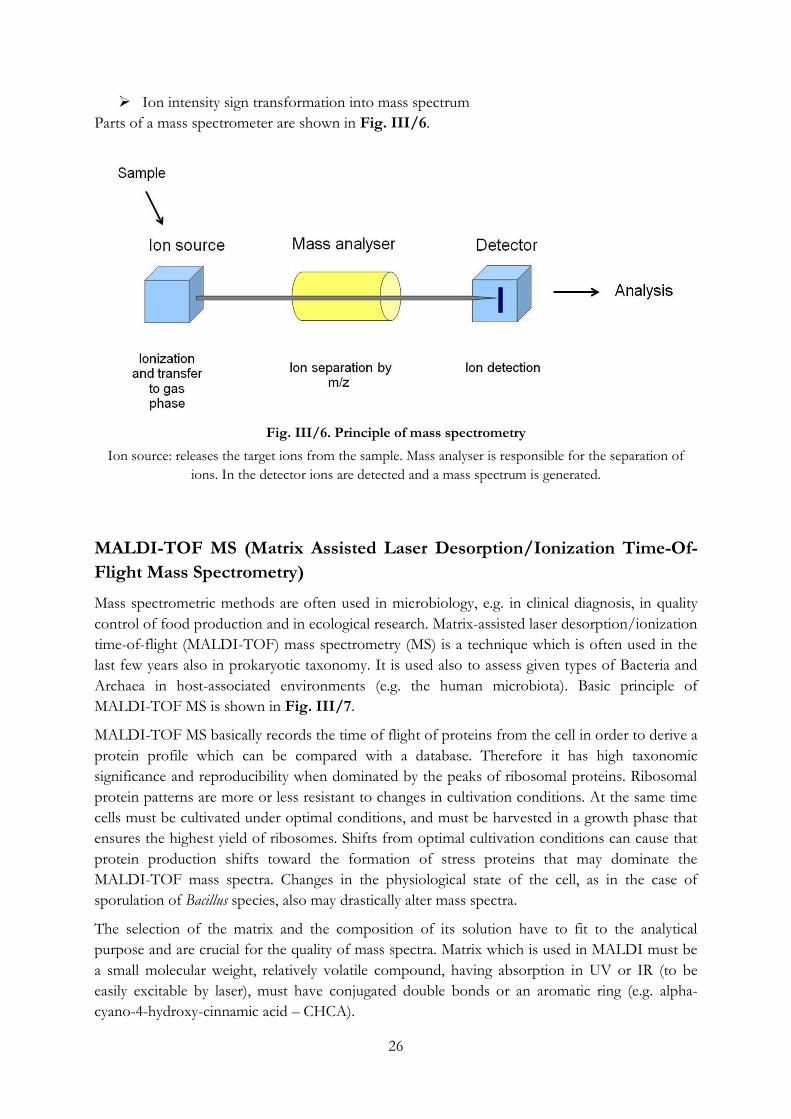
Ion intensity sign transformation into mass spectrum
Parts of a mass spectrometer are shown in Fig. III/6.
Fig. III/6. Principle of mass spectrometry
Ion source: releases the target ions from the sample. Mass analyser is responsible for the separation of
ions. In the detector ions are detected and a mass spectrum is generated.
MALDI-TOF MS (Matrix Assisted Laser Desorption/Ionization Time-Of-
Flight Mass Spectrometry)
Mass spectrometric methods are often used in microbiology, e.g. in clinical diagnosis, in quality
control of food production and in ecological research. Matrix-assisted laser desorption/ionization
time-of-flight (MALDI-TOF) mass spectrometry (MS) is a technique which is often used in the
last few years also in prokaryotic taxonomy. It is used also to assess given types of Bacteria and
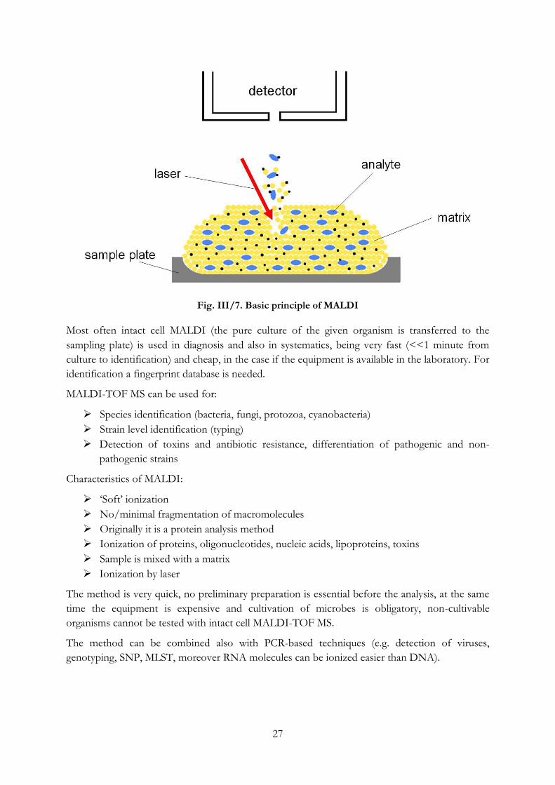
Archaea in host-associated environments (e.g. the human microbiota). Basic principle of
MALDI-TOF MS is shown in Fig. III/7.
MALDI-TOF MS basically records the time of flight of proteins from the cell in order to derive a
protein profile which can be compared with a database. Therefore it has high taxonomic
significance and reproducibility when dominated by the peaks of ribosomal proteins. Ribosomal
protein patterns are more or less resistant to changes in cultivation conditions. At the same time
cells must be cultivated under optimal conditions, and must be harvested in a growth phase that
ensures the highest yield of ribosomes. Shifts from optimal cultivation conditions can cause that
protein production shifts toward the formation of stress proteins that may dominate the
MALDI-TOF mass spectra. Changes in the physiological state of the cell, as in the case of
sporulation of Bacillus species, also may drastically alter mass spectra.
The selection of the matrix and the composition of its solution have to fit to the analytical
purpose and are crucial for the quality of mass spectra. Matrix which is used in MALDI must be
a small molecular weight, relatively volatile compound, having absorption in UV or IR (to be
easily excitable by laser), must have conjugated double bonds or an aromatic ring (e.g. alpha-
cyano-4-hydroxy-cinnamic acid – CHCA).
27
Fig. III/7. Basic principle of MALDI
Most often intact cell MALDI (the pure culture of the given organism is transferred to the
sampling plate) is used in diagnosis and also in systematics, being very fast (<<1 minute from
culture to identification) and cheap, in the case if the equipment is available in the laboratory. For
identification a fingerprint database is needed.
MALDI-TOF MS can be used for:
Species identification (bacteria, fungi, protozoa, cyanobacteria)
Strain level identification (typing)
Detection of toxins and antibiotic resistance, differentiation of pathogenic and non-
pathogenic strains
Characteristics of MALDI:
‘Soft’ ionization
No/minimal fragmentation of macromolecules
Originally it is a protein analysis method
Ionization of proteins, oligonucleotides, nucleic acids, lipoproteins, toxins
Sample is mixed with a matrix
Ionization by laser
The method is very quick, no preliminary preparation is essential before the analysis, at the same
time the equipment is expensive and cultivation of microbes is obligatory, non-cultivable
organisms cannot be tested with intact cell MALDI-TOF MS.
The method can be combined also with PCR-based techniques (e.g. detection of viruses,
genotyping, SNP, MLST, moreover RNA molecules can be ionized easier than DNA).
28
III.7. Community level chemotaxonomic analysis
Chemotaxonomic analyses can be used to study also microbial communities of various sources
(e.g. soils, wastewaters) where their biomass is high enough, as in chemotaxonomy there is no
amplification of the target molecules. Markers are extracted directly from the samples and after
purification of the components chromatographic analysis is applied (GC, HPLC). Fatty acids and
respiratory quinones can be examined in more details. There are some universal markers, which
do not give information about the structure of the community, as they are present also in plants,
fungi and other eukaryotic cells. But there are some specific molecules which can be
characteristic for different ranks of bacteria (e.g. OH-fatty acids are markers of Gram-negative
bacteria, iso and anteiso branching fatty acids are characteristic for Gram-positives). The analysis
of quinone compounds can give information also about the activity of a given community: being
parts of the respiratory chain of different organisms, in detectable amounts they can be
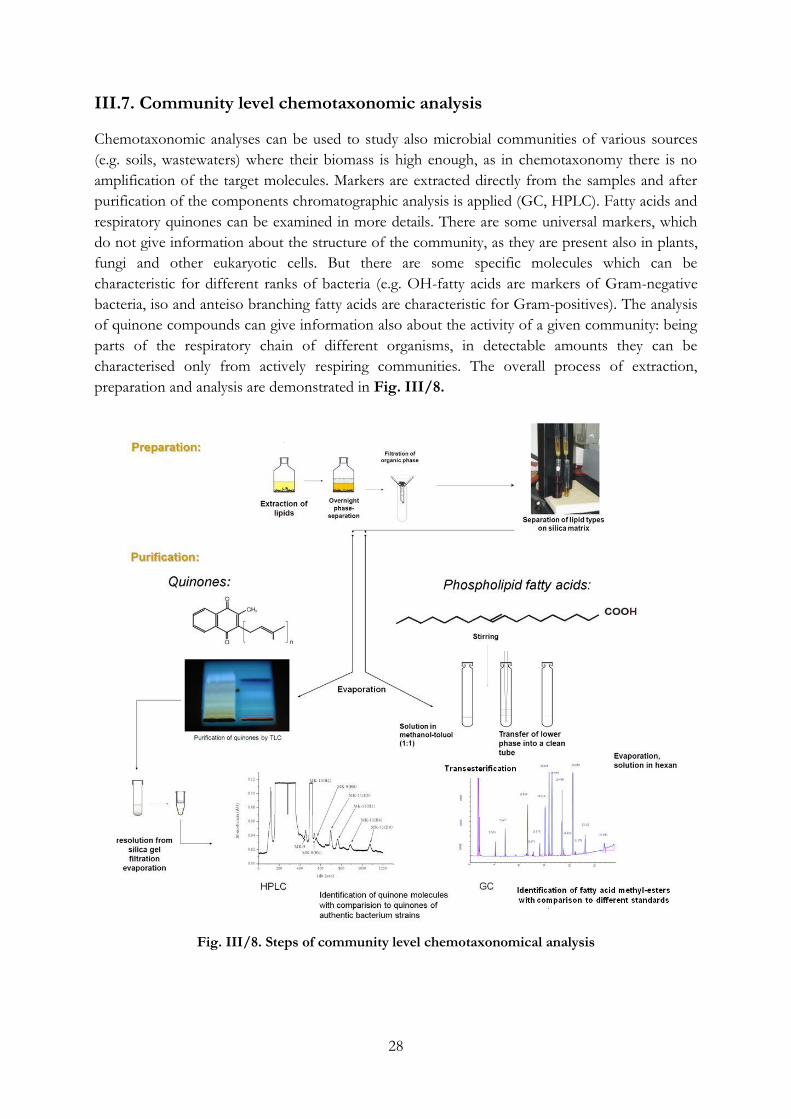
characterised only from actively respiring communities. The overall process of extraction,
preparation and analysis are demonstrated in Fig. III/8.
Fig. III/8. Steps of community level chemotaxonomical analysis
29
IV. NUCLEIC ACID BASED TECHNIQUES USED IN
BACTERIAL TAXONOMY AND MICROBIAL
ECOLOGY (Balázs Vajna, Tamás Felföldi)
Nucleic acids are the information carrying molecules of all living creatures. While DNA stands
for long-term information storage within the cell, RNA shows the actually expressed information.
In other words, DNA represents possibilities, while RNA represents realisation. But it should be
noted that there are several steps from transcribed RNA to functional proteins, which means, not
even RNA should be regarded as direct functional information. From most samples both DNA
and RNA can be extracted but in this practical guide we will focus mainly on DNA-based
analysis.
Nucleic acid based information can be used for two basic approaches. First approach is to
identify bacterial strains or community members mainly on the basis of the 16S rRNA gene.
Identifying bacteria from communities is extremely important since we know that usually less
than 1-10% of bacteria can be cultivated from most of the environments. Second approach is a
functional one, when the possible functions of a bacterial community or a strain are checked
based on the presence of genes coding the function.
In the following we describe the basic steps from the isolation of nucleic acids till the analysis of
sequence information. Most of the steps are applicable both on community and on strain level.
We summarize separate pipelines for species description and for studies of environmental
samples in Chapter VII and IV.8.
List of materials and equipment necessary for every exercise in Chapter IV. Thus they will not be listed at each
exercise again.
micropipettes, sterile pipette tips
microcentrifuge and PCR tubes
microcentrifuge tube rack
microcentrifuge
vortex mixer
molecular biology grade water (marked simply H2O in this chapter)
IV.1. Separation of nucleic acids
Separation of nucleic acids has several aims. Usually the size of the DNA should be determined
and compared with the expected length of the molecule, but these methods can be used also for
fingerprint generation and purification. Three main techniques are applied: agarose,
polyacrylamide and capillary gel electrophoresis.
30
Agarose is a polysaccharide polymer built up from agarobiose disaccharides forming helical
fibres, which aggregate into supercoiled structure. The resulted three-dimensional mesh forms
channels with diameters depending on the concentration of the used agarose. By polyacrylamide
and capillary gel electrophoresis the gel is built up from polymerised and partially covalently
crosslinked acrylamide and bisacrylamide molecules. In both cases the higher the percentage of
agarose or acrylamide is, the higher the resolution of the gel is.
Agarose has the lowest resolution, not more than 10 bp for 1 kb range, but it is the easiest gel to
handle. Capillary electrophoresis on the other side has a 1 bp resolution but it needs much more
equipment. The required resolution of the electrophoresis usually depends on the question to be
answered. For confirmation of the proper size of a desired PCR product agarose gel
electrophoresis is generally satisfactory, whereas for high resolution pattern-analysis or separation
of cycle sequencing products polyacrylamide (with a resolution of 1 bp) or capillary gel
electrophoresis is needed.
Agarose and polyacrylamide gel electrophoresis can also be used for purification of the DNA
sample, where the nucleic acid band with the desired size can be excised and purified from the
gel. A specific DNA sequence can be identified with agarose gel electrophoresis via Southern
blot.
DNA is visualized during or after the agarose and polyacrylamide gel electrophoresis with
fluorescent nucleic acid dyes (such as ethidium bromide, SYBR Green, GR safe), usually
intercalating into nucleic acids. Ethidium bromide is highly mutagenic, thus it is rarely used
nowadays. Nevertheless every dye should be handled with care because their ability of binding to
the DNA. At capillary electrophoresis, DNA fragments are fluorescently labelled and detected
near to the end of the capillary via laser-induced fluorescence.
It should be noted, that nucleic acids can be separated via column chromatography, as well. This
technique is used also as a part of the purification of the isolated nucleic acid and will be detailed
in Chapter IV.2.
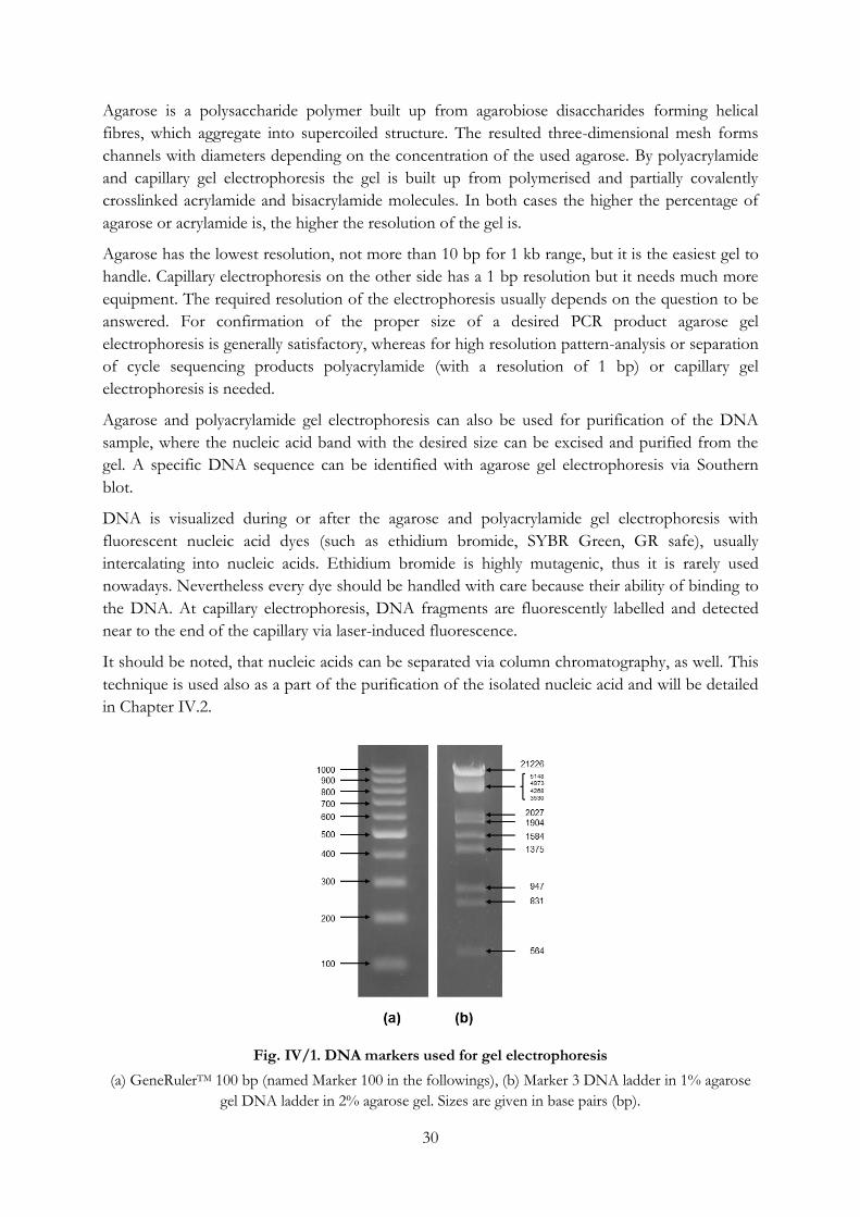
Fig. IV/1. DNA markers used for gel electrophoresis
(a) GeneRulerTM 100 bp (named Marker 100 in the followings), (b) Marker 3 DNA ladder in 1% agarose
gel DNA ladder in 2% agarose gel. Sizes are given in base pairs (bp).
31
EXERCISE IV/1.: Agarose gel electrophoresis
This technique is used for checking the integrity and intensity of isolated genomic or
environmental DNA, comparing the size of the PCR product with the desired value, checking its
intensity and analysing basic fingerprints (ARDRA, RAPD, etc.).
Object of study
bacterial genomic DNA, environmental DNA samples, PCR products
Materials and equipment
laboratory scales
measuring cylinder
250 mL flask
horizontal agarose gel electrophoresis system
gel casting system
agarose
1× TBE (Tris-Borate-EDTA) buffer
DNA stain (GR Safe nucleic acid stain)
loading buffer
Parafilm
DNA ladder (e.g. Marker 3, GeneRulerTM 100 bp DNA ladder, Fig. IV/1.)
gel documentation system
Procedure
1. The first step of agarose gel electrophoresis is gel preparation and casting. The percentage of
agarose depends on the required resolution (see below). In case of 1% agarose gel, add 80
mL 1× TBE solution to 0.8 g agarose. Boil it until the agarose is completely dissolved, cool
to approx. 60 °C, and add 1.5 μL DNA stain to the solution and mix. Insert combs into the
gel casting system, and pour the agarose solution into it without creating bubbles.
2. When the gel has solidified (requires 30-40 minutes), remove combs, and place the gel into
the buffer tank of the electrophoresis apparatus filled previously with 1× TBE solution.
3. Mix 5 μL DNA sample with 3 μL loading buffer on a piece of Parafilm, and load this
mixture into the wells of the gel. To achieve a semi-quantitative measurement of the intensity
and size of DNA, load 2 μL appropriate DNA ladder next to the samples.
4. Run electrophoresis for the desired time at the desired voltage.
Type of
electrophoresis
% of the gel (agarose in
80 mL 1× TBE buffer)
Length of the
electrophoresis1
Voltage of the
electrophoresis1
General 1% (0.8 g) 20 min. 100 V
ARDRA 2% (1.6 g) 80 min. 80 V
RAPD, ITS-PCR 2% (1.6 g) 180 min. 80 V
1when using 14 cm long gel
5. Detect the presence and quantity of DNA under UV light. Compare the quality (discrete
bands or smears; size of the DNA) and quantity (intensity of the signal) of the DNA samples
with the ladder. Obtain a digital image if needed for documentation or image analysis.
32
EXERCISE IV/2.: Polyacrylamide gel electrophoresis (PAGE)
This technique is preferred, when higher resolution than agarose gel electrophoresis is needed
(<10 bp), and/or the dominant DNA bands from a sample with many bands are needed to be
separated and isolated. Traditionally polyacrylamide gel was used for Sanger sequencing. A
modified version, DGGE (Chapter IV.7.) is used for comparing complex environmental
fingerprints.
Object of study
bacterial genomic DNA, environmental DNA samples, PCR products
Materials and equipment
measuring cylinder
50-mL Falcon tube
40% acrylamide solution (acrylamide : bisacrylamide – 37.5:1)
50× TAE (Tris-Acetate-EDTA) buffer
ddH2O (double distilled water)
TEMED (tetramethylethylenediamine)
20% ammonium-persulfate (APS) solution
polyacrylamide gel electrophoresis system (Ingeny phorU-2) with gel casting system
loading dye
Hamilton syringe
DNA ladder (e.g. Marker 3, Marker 100, Fig. IV/1.)
gel staining box
DNA stain (ethidium-bromide solution)
scalpel
gel documentation system
computer with Totallab software
Procedure
1. Assemble the electrophoresis system as described in its manual.
2. Prepare 30 mL of 10% acrylamide solution in a 50-mL Falcon tube: mix 7.5 mL 40%
acrylamide solution, 0.6 mL 50× TAE buffer and 21.9 mL ddH2O. Add 60 µL APS solution
and 25 µL TEMED to it, load it to the gel casting system and insert combs. Wait 2 hours for
the polymerisation. (Acrylamide is toxic! Handle it carefully according to its safety data
sheet!)
3. Put the gel casting system into the buffer tank of the electrophoresis apparatus filled
previously with 1× TAE solution, and remove gently the combs. Wash the wells with
1× TAE solution using a Hamilton syringe in order to remove unpolymerised acrylamide
particles.
4. Mix 10 µL DNA sample with 2 µL loading dye and load it with a Hamilton syringe into the
wells of the gel. To achieve a semi-quantitative measurement of the intensity and size of
DNA, load 10 μL appropriate DNA ladder next to the samples.
5. Run the electrophoresis at 250 V for 105 minutes.
33
6. After electrophoresis disassemble the gel electrophoresis system, stain the gel in ethidium-
bromide solution for 20 minutes, and destain it for two times with incubation for 15-15
minutes in 1× TAE buffer. (Ethidium-bromide is toxic! Handle it carefully according to its
safety data sheet!)
7. Detect the presence and quantity of DNA under UV light and obtain a digital image. The
image can be analysed with adequate software (e.g. Totallab).
8. If excision of dominant bands is needed, cut them out with a sterile scalpel, and put them
into 30 µL H2O in an Eppendorf tube. Incubate at 4 °C overnight, thereafter transfer the
liquid part into a new tube. Now it is ready for PCR or store at -20 °C for longer time.
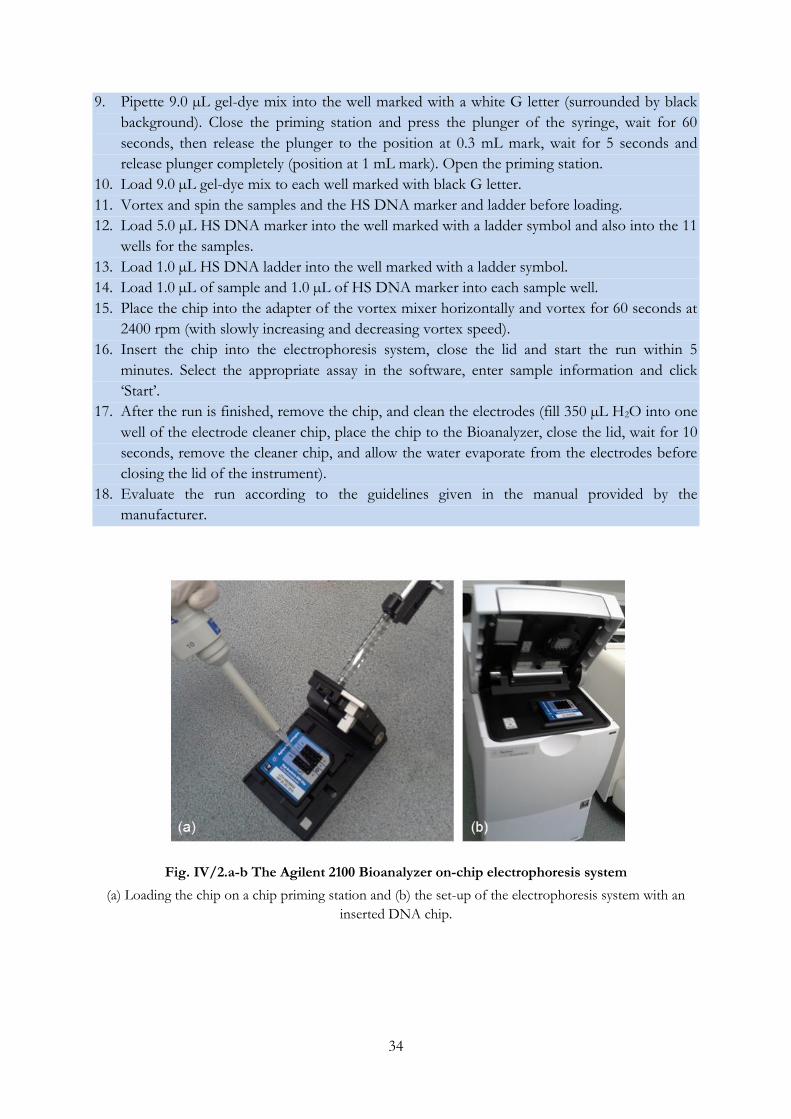
EXERCISE IV/3.: Separation of DNA molecules with a model 2100 Bioanalyzer (Agilent
Technologies)
Agilent 2100 Bioanalyzer is an on-chip capillary electrophoresis system (Fig. IV/2.), which
provides sizing, quantitation and quality control of DNA. Chips are commercially available for
the analysis of RNA molecules and proteins, as well. In the case of DNA analysis, usually only 1
µL of sample is required and the resolution of ~5 bp can be achieved.
Object of study
bacterial genomic DNA, environmental DNA samples, PCR products
Materials and equipment
Agilent 2100 Bioanalyzer
chip priming station
Agilent High Sensitivity (HS) DNA kit:
DNA chips, electrode cleaner, DNA marker (mixture of two marker with sizes of
35 and 10,380 bp), dye concentrate, syringe, gel matrix, DNA ladder (mixture of 13 DNA
fragments having different size), spin filters, electrode cleaner chip
vortex mixer (IKA Model MS3 equipped with the proper chip adapter)
PC equipped with the adequate software (2100 Expert)
Procedure
1. Allow the HS DNA dye concentrate and HS DNA gel matrix to equilibrate to room
temperature (this takes approximately 30 minutes, protect from light).
2. Replace the syringe in the chip priming station: unscrew and discard the old syringe, remove
the plastic cap of the new syringe and insert it into the clip, then screw the new syringe to the
chip priming station.
3. Adjust the base plate in the chip priming station to position C and slide the lever of the clip
down to the lowest position. The plunger of the syringe should be positioned at 1 mL mark.
4. Start the 2100 Expert software on the PC, check the connection between the instrument and
the PC.
5. Vortex HS DNA dye concentrate for 10 seconds and then spin down.
6. Pipette 15 µL HS DNA dye concentrate into the HS DNA gel matrix and mix by vortexing.
7. Transfer the mixture to the spin filter, centrifuge for 13 minutes at 5500 g. Discard the filter.
8. Take a new chip out of the sealed bag and place it to the chip priming station.
34
9. Pipette 9.0 µL gel-dye mix into the well marked with a white G letter (surrounded by black
background). Close the priming station and press the plunger of the syringe, wait for 60
seconds, then release the plunger to the position at 0.3 mL mark, wait for 5 seconds and
release plunger completely (position at 1 mL mark). Open the priming station.
10. Load 9.0 µL gel-dye mix to each well marked with black G letter.
11. Vortex and spin the samples and the HS DNA marker and ladder before loading.
12. Load 5.0 µL HS DNA marker into the well marked with a ladder symbol and also into the 11
wells for the samples.
13. Load 1.0 µL HS DNA ladder into the well marked with a ladder symbol.
14. Load 1.0 µL of sample and 1.0 µL of HS DNA marker into each sample well.
15. Place the chip into the adapter of the vortex mixer horizontally and vortex for 60 seconds at
2400 rpm (with slowly increasing and decreasing vortex speed).
16. Insert the chip into the electrophoresis system, close the lid and start the run within 5
minutes. Select the appropriate assay in the software, enter sample information and click
‘Start’.
17. After the run is finished, remove the chip, and clean the electrodes (fill 350 µL H2O into one
well of the electrode cleaner chip, place the chip to the Bioanalyzer, close the lid, wait for 10
seconds, remove the cleaner chip, and allow the water evaporate from the electrodes before
closing the lid of the instrument).
18. Evaluate the run according to the guidelines given in the manual provided by the
manufacturer.
Fig. IV/2.a-b The Agilent 2100 Bioanalyzer on-chip electrophoresis system
(a) Loading the chip on a chip priming station and (b) the set-up of the electrophoresis system with an
inserted DNA chip.
35
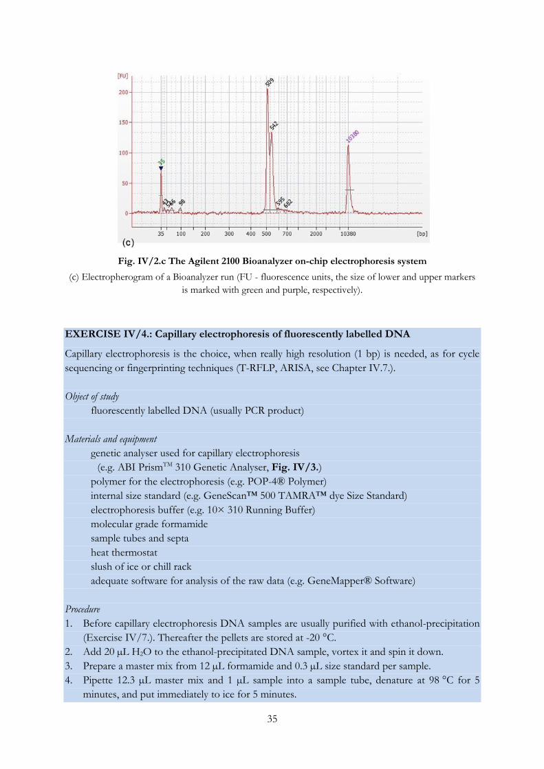
Fig. IV/2.c The Agilent 2100 Bioanalyzer on-chip electrophoresis system
(c) Electropherogram of a Bioanalyzer run (FU - fluorescence units, the size of lower and upper markers
is marked with green and purple, respectively).
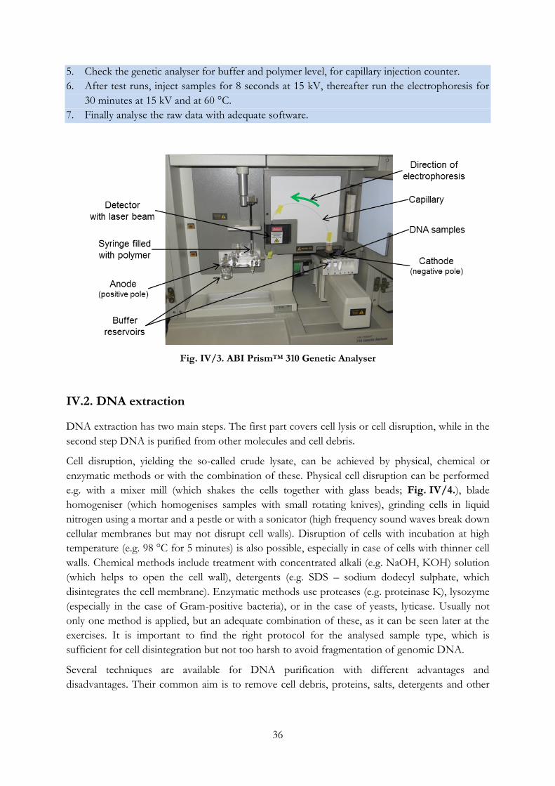
EXERCISE IV/4.: Capillary electrophoresis of fluorescently labelled DNA
Capillary electrophoresis is the choice, when really high resolution (1 bp) is needed, as for cycle
sequencing or fingerprinting techniques (T-RFLP, ARISA, see Chapter IV.7.).
Object of study
fluorescently labelled DNA (usually PCR product)
Materials and equipment
genetic analyser used for capillary electrophoresis
(e.g. ABI PrismTM 310 Genetic Analyser, Fig. IV/3.)
polymer for the electrophoresis (e.g. POP-4® Polymer)
internal size standard (e.g. GeneScan™ 500 TAMRA™ dye Size Standard)
electrophoresis buffer (e.g. 10× 310 Running Buffer)
molecular grade formamide
sample tubes and septa
heat thermostat
slush of ice or chill rack
adequate software for analysis of the raw data (e.g. GeneMapper® Software)
Procedure
1. Before capillary electrophoresis DNA samples are usually purified with ethanol-precipitation
(Exercise IV/7.). Thereafter the pellets are stored at -20 °C.
2. Add 20 µL H2O to the ethanol-precipitated DNA sample, vortex it and spin it down.
3. Prepare a master mix from 12 µL formamide and 0.3 µL size standard per sample.
4. Pipette 12.3 µL master mix and 1 µL sample into a sample tube, denature at 98 °C for 5
minutes, and put immediately to ice for 5 minutes.
36
5. Check the genetic analyser for buffer and polymer level, for capillary injection counter.
6. After test runs, inject samples for 8 seconds at 15 kV, thereafter run the electrophoresis for
30 minutes at 15 kV and at 60 °C.
7. Finally analyse the raw data with adequate software.
Fig. IV/3. ABI PrismTM 310 Genetic Analyser
IV.2. DNA extraction
DNA extraction has two main steps. The first part covers cell lysis or cell disruption, while in the
second step DNA is purified from other molecules and cell debris.
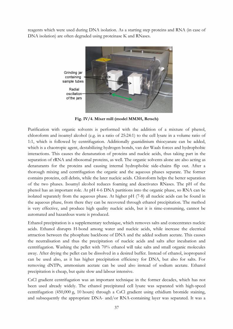
Cell disruption, yielding the so-called crude lysate, can be achieved by physical, chemical or
enzymatic methods or with the combination of these. Physical cell disruption can be performed
e.g. with a mixer mill (which shakes the cells together with glass beads; Fig. IV/4.), blade
homogeniser (which homogenises samples with small rotating knives), grinding cells in liquid
nitrogen using a mortar and a pestle or with a sonicator (high frequency sound waves break down
cellular membranes but may not disrupt cell walls). Disruption of cells with incubation at high
temperature (e.g. 98 °C for 5 minutes) is also possible, especially in case of cells with thinner cell
walls. Chemical methods include treatment with concentrated alkali (e.g. NaOH, KOH) solution
(which helps to open the cell wall), detergents (e.g. SDS – sodium dodecyl sulphate, which
disintegrates the cell membrane). Enzymatic methods use proteases (e.g. proteinase K), lysozyme
(especially in the case of Gram-positive bacteria), or in the case of yeasts, lyticase. Usually not
only one method is applied, but an adequate combination of these, as it can be seen later at the
exercises. It is important to find the right protocol for the analysed sample type, which is
sufficient for cell disintegration but not too harsh to avoid fragmentation of genomic DNA.
Several techniques are available for DNA purification with different advantages and
disadvantages. Their common aim is to remove cell debris, proteins, salts, detergents and other
37
reagents which were used during DNA isolation. As a starting step proteins and RNA (in case of
DNA isolation) are often degraded using proteinase K and RNases.
Fig. IV/4. Mixer mill (model MM301, Retsch)
Purification with organic solvents is performed with the addition of a mixture of phenol,
chloroform and isoamyl alcohol (e.g. in a ratio of 25:24:1) to the cell lysate in a volume ratio of
1:1, which is followed by centrifugation. Additionally guanidinium thiocyanate can be added,
which is a chaotropic agent, destabilizing hydrogen bonds, van der Waals forces and hydrophobic
interactions. This causes the denaturation of proteins and nucleic acids, thus taking part in the
separation of rRNA and ribosomal proteins, as well. The organic solvents alone are also acting as
denaturants for the proteins and causing internal hydrophobic side-chains flip out. After a
thorough mixing and centrifugation the organic and the aqueous phases separate. The former
contains proteins, cell debris, while the later nucleic acids. Chloroform helps the better separation
of the two phases. Isoamyl alcohol reduces foaming and deactivates RNases. The pH of the
phenol has an important role. At pH 4-6 DNA partitions into the organic phase, so RNA can be
isolated separately from the aqueous phase. At higher pH (7-8) all nucleic acids can be found in
the aqueous phase, from there they can be recovered through ethanol precipitation. The method
is very effective, and produce high quality nucleic acids, but it is time-consuming, cannot be
automated and hazardous waste is produced.
Ethanol precipitation is a supplementary technique, which removes salts and concentrates nucleic
acids. Ethanol disrupts H-bond among water and nucleic acids, while increase the electrical
attraction between the phosphate backbone of DNA and the added sodium acetate. This causes
the neutralisation and thus the precipitation of nucleic acids and salts after incubation and
centrifugation. Washing the pellet with 70% ethanol will take salts and small organic molecules
away. After drying the pellet can be dissolved in a desired buffer. Instead of ethanol, isopropanol
can be used also, as it has higher precipitation efficiency for DNA, but also for salts. For
removing dNTPs, ammonium acetate can be used also instead of sodium acetate. Ethanol
precipitation is cheap, but quite slow and labour intensive.
CsCl gradient centrifugation was an important technique in the former decades, which has not
been used already widely. The ethanol precipitated cell lysate was separated with high-speed
centrifugation (450,000 g, 10 hours) through a CsCl gradient using ethidium bromide staining,
and subsequently the appropriate DNA- and/or RNA-containing layer was separated. It was a
38
suitable method to separate nuclear and mitochondrial DNA, as the DNA was protected from
fragmentation. After a further ethanol precipitation of the target, the method yielded very pure
DNA. On the other hand, the procedure was time-consuming, expertise and special equipment
were required, and hazardous waste was produced.
One of the most widespread techniques today is the silicate-based methods applied in many
commercial kits as final purification steps. It exploits the selective binding of nucleic acids to a
silicate gel at high concentration of chaotropic salts (e.g. sodium persulphate, lithium chloride). In
the next steps a selective washing procedure is used. First washing contains low amount of
chaotropic salt to remove proteins and coloured contaminants. The second washing is usually
ethanol to remove salts. After proper drying of the gel, nucleic acids could be eluted. In case of
RNA isolation, elution is achieved by application of a buffer with pH 4-5, while for DNA the pH
of the buffer is typically 8-9. This means also, that both nucleic acids can be eluted selectively
after each other with the adequate buffers. The silicate-based methods yield pure DNA, free
from small fragments, but the method is not suitable for the purification of very large DNA
molecules.
New techniques for nucleic acid purification are developed constantly. One approach uses
magnetic beads that bind DNA conditionally and can be immobilized on a magnet to separate
the DNA from the rest of the sample. The beads are positively charged at low pH, and will
therefore bind to DNA, but at high pH they are negatively charged and release the DNA. It is
fast, uses no chaotrophic salts or organic washing solutions, and yields high purity DNA. Its
disadvantages are that the initial outlay for the magnets is relative high and the procedure is a bit
tricky when handling multiple samples.
Further aspects should be considered when nucleic acids are isolated not from cell cultures but
from environmental samples. Two basic approaches exist. One is the a priori separation of cells
from the sample with e.g. Nycodenz® gradient centrifugation. Less fragmented and less
contaminated DNA can be obtained, but a fraction of the cells is lost during separation. The
second approach is direct lysis of the bacterial cells in the sample matrix, thereafter isolation and
purification of the released nucleic acids happen as described above. Sample matrix can cause
problem, as e.g. humic substances, clay minerals in soil tend to bind DNA, which inhibit
downstream reaction. Therefore the application of different inhibitor removing steps is required.
PVPP (polyvinylpolypyrrolidone), which is a highly cross-linked modification of the polymerised
N-vinylpyrrolidone, for example binds phenolic compounds, which can be removed thereafter
with centrifugation. Another problem is, that direct lysis does not distinguish between cellular
and free DNA, the later derive from previously dead cells. Direct lysis yields generally higher
amount of DNA, but could be more fragmented.
If using a new type of sample, it is worth comparing the result of different DNA isolation and
purification techniques. Often some kind of optimisation or fine tuning of the previously applied
protocol is needed. When we handle environmental samples, we should be aware that there is no
method, which is equally efficient for all kind of bacteria. Thus every DNA isolation method
distorts the original community composition in some degree. As DNA extraction is the first step
in every nucleic acid based technique, its accuracy or at least its reproducibility has utmost
importance.
39
Final task of DNA isolation is the quality- and quantity-check. Low quality DNA contains other
molecules from the original sample (e.g. proteins, humic substances) or contaminants from the
isolation workflow (e.g. salts, phenols, ethanol or detergents). All these substances can hinder
subsequent applications. DNA purity can be checked by e.g. spectrophotometric analysis, and
described with the ratio of measured absorbance at 260 and 280 nm. If this value is higher than
1.7, the purity of the DNA can be accepted. The result of DNA extraction can be checked with
agarose gel electrophoresis, as well, especially if fragmentation is important. For really higher
resolution, the Bioanalyzer should be used. To avoid degradation, DNA should be kept in a
freezer (at -20 °C).
Different DNA characterisation methods need different DNA quantities. Also the copy number
of the target gene is important. rRNA operons (containing 16S rRNA gene) usually occurs in
more than one copy in the genome, which means, lower amount of DNA is enough to reach the
threshold of detection in a PCR. The quantity of sample used for DNA extraction depends on
the DNA content of the individual cells. Recommended cell numbers used for DNA isolation are
109 cells for bacteria, 107 cells for yeasts and 106 cells for animal cell cultures.
EXERCISE IV/5.: DNA extraction from bacterial cells with different techniques
Object of study
slant cultures of bacteria
Materials and equipment
inoculating loop
0.5 M NaOH solution
1 M TRIS [Tris(hydroxymethyl)aminomethane] buffer (pH 8.0)
mixer mill (bead beater)
thermocycler or water bath
sterile glass beads
DNA isolation kit (e.g. G-spin™ Total DNA Extraction Mini Kit)
Procedure
Three DNA isolation procedures differing in their cell lysis and purification steps are performed
in parallel.
Chemical lysis with NaOH solution:
1. Measure 25 μL 0.5 M NaOH solution into a 1.5 mL microcentrifuge tube that is labelled
with the name of the bacterium strain.
2. Suspend a loopful of bacteria in the solution, vortex thoroughly, spin it down and incubate
for 15 minutes at room temperature.
3. Add 25 μL 1 M TRIS buffer and 300 μL H2O.
Physical lysis with thermal denaturation:
1. Measure 100 μL sterile glass beads, 8 μL 1 M TRIS buffer and 100 μL H2O into a 600 μL
microcentrifuge tube that is labelled with the name of the bacterium strain.
2. Suspend a loopful of bacteria and shake the tubes for 1 minute at 30 Hz in a mixer mill.
40
3. Spin the tubes quickly, and incubate for 5 minutes at 98 °C (in a thermocycler or in a water
bath).
4. Vortex for 5 seconds, centrifuge the tubes for 5 minutes at 10,000 g and transfer the
supernatant (approx. 70 μL) to a new, labelled microcentrifuge tube.
Using a commercial DNA isolating kit:
This kit is based on enzymatic lysis of the cells followed by a silica-column purification of the
DNA.
To complete the procedure, follow the instructions given by the manufacturer at protocol F.
Check the DNA quality of all samples with agarose gel electrophoresis (Exercise IV/1.).
Store isolated DNA at -20 °C for further analysis.
EXERCISE IV/6.: DNA extraction from environmental samples with different
techniques
Object of study
environmental samples
Materials and equipment
sterile spatula and tweezer
0.45 μm cellulose nitrate membrane filter
sterile, membrane filtration equipment (Millipore)
DNA isolation kit (e.g. UltraClean® Soil DNA Isolation Kit)
mixer mill (bead beater)
thermocycler or water bath
liquid N2
sterile mortar and pestle
lysis buffer (CLS-TC or CLS-Y, component of the FastDNA® Kit)
PVPP
DNA isolation kit (e.g. G-spin™ Total DNA Extraction Mini Kit)
Procedure
Two DNA isolation procedures are performed in parallel that differ in their cell lysis and
purification steps.
UltraClean® Soil DNA Isolation Kit for soil and water samples:
This kit is based on physical and chemical lysis using ceramic beads and SDS, thereafter patented
inhibitor removal techniques and silica-column purification are applied.
1. Soil sample can be added directly to the kit.
2. Cells from water samples (0.1-10 L depending on density) should be concentrated by
filtration through a 0.22 µm pore-sized cellulose nitrate membrane filter. Then filters cut into
smaller pieces can be added to the bead tube of the kit.
3. Then follow the instructions given by the manufacturer.
4. The only modification is, that instead a vortex adapter, use a mixer mill for 2 minute at 30
Hz.
41
Physical lysis using liquid N2:
This procedure can be used as an alternative for the above kit, when we have samples with many
endospores or thick cell-wall bacteria.
1. For each sample, pipette 1 mL CLS-TC or CLS-Y lysis buffer into a 1600 μL labelled
microcentrifuge tube and add about 50 mg PVPP powder to it. CLS-TC is a lysis buffer
developed for bacteria and cells from tissue cultures, whereas CLS-Y for yeast, algae and
fungi.
2. Pour liquid N2 into the sterile mortar. (Handle liquid N2 always carefully according to safety
regulations.)
3. With sterile tweezer and spatula add 1 g sample into the mortar filled with the liquid N2 and
ground it thoroughly.
4. Refill the mortar with liquid N2 if evaporated and continue the grinding until the sample will
form a homogenous powder. (At the first application of the method, the length of the
homogenisation should be optimized, to reach sufficient cell disintegration without
fragmentation of genomic DNA, as mentioned above in the introduction.)
5. Centrifuge the sample tubes for 8 minutes at 15,500 g and transfer supernatant (the crude
lysate) to a new labelled microcentrifuge tube.
6. The crude lysate can be purified in several ways. One option is to use the G-spin™ Total
DNA Extraction Mini Kit protocol F from step 4.
Check the DNA quality of all samples with agarose gel electrophoresis (Exercise IV/1.).
Store isolated DNA at -20 °C for further analysis.
EXERCISE IV/7.: DNA purification with ethanol precipitation
Object of study
bacterial genomic DNA, environmental DNA samples, PCR products
Materials and equipment
3 M Na-acetate solution (pH 4.6)
95% ethanol and 70% ethanol
microcentrifuge (refrigerated)
vacuum centrifuge
Procedure
1. Prepare a master mix: add 62.5 μL 95% ethanol, 3.0 μL 3 M Na-acetate and 14.5 μL H2O per
reaction into a 1.5 mL microcentrifuge tube, multiply the given amount by sample number
plus one.
2. Pipette 80 μL from this master mix to each labelled 0.6 mL microcentrifuge tube containing
the DNA sample.
3. Vortex the tubes vigorously, then incubate at room temperature for 15 minutes.
4. Centrifuge the tubes for 20 minutes at 18,000 g at 4 °C, and carefully remove the supernatant
by pipetting.
5. Add 250 μL 70% ethanol, vortex the tubes vigorously, and centrifuge at 18,000 g for 10
minutes. Remove the supernatant by pipetting.
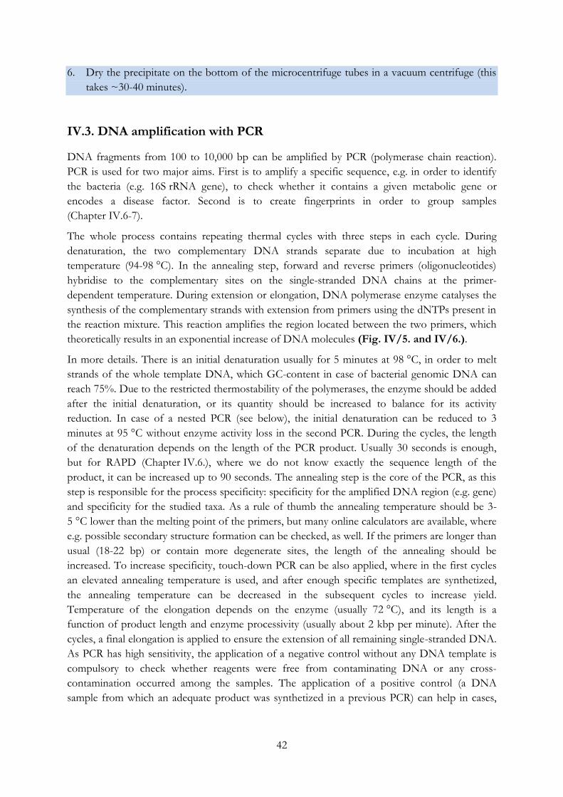
42
6. Dry the precipitate on the bottom of the microcentrifuge tubes in a vacuum centrifuge (this
takes ~30-40 minutes).
IV.3. DNA amplification with PCR
DNA fragments from 100 to 10,000 bp can be amplified by PCR (polymerase chain reaction).
PCR is used for two major aims. First is to amplify a specific sequence, e.g. in order to identify
the bacteria (e.g. 16S rRNA gene), to check whether it contains a given metabolic gene or
encodes a disease factor. Second is to create fingerprints in order to group samples
(Chapter IV.6-7).
The whole process contains repeating thermal cycles with three steps in each cycle. During
denaturation, the two complementary DNA strands separate due to incubation at high
temperature (94-98 °C). In the annealing step, forward and reverse primers (oligonucleotides)
hybridise to the complementary sites on the single-stranded DNA chains at the primer-
dependent temperature. During extension or elongation, DNA polymerase enzyme catalyses the
synthesis of the complementary strands with extension from primers using the dNTPs present in
the reaction mixture. This reaction amplifies the region located between the two primers, which
theoretically results in an exponential increase of DNA molecules (Fig. IV/5. and IV/6.).
In more details. There is an initial denaturation usually for 5 minutes at 98 °C, in order to melt
strands of the whole template DNA, which GC-content in case of bacterial genomic DNA can
reach 75%. Due to the restricted thermostability of the polymerases, the enzyme should be added
after the initial denaturation, or its quantity should be increased to balance for its activity
reduction. In case of a nested PCR (see below), the initial denaturation can be reduced to 3
minutes at 95 °C without enzyme activity loss in the second PCR. During the cycles, the length
of the denaturation depends on the length of the PCR product. Usually 30 seconds is enough,
but for RAPD (Chapter IV.6.), where we do not know exactly the sequence length of the
product, it can be increased up to 90 seconds. The annealing step is the core of the PCR, as this
step is responsible for the process specificity: specificity for the amplified DNA region (e.g. gene)
and specificity for the studied taxa. As a rule of thumb the annealing temperature should be 3-
5 °C lower than the melting point of the primers, but many online calculators are available, where
e.g. possible secondary structure formation can be checked, as well. If the primers are longer than
usual (18-22 bp) or contain more degenerate sites, the length of the annealing should be
increased. To increase specificity, touch-down PCR can be also applied, where in the first cycles
an elevated annealing temperature is used, and after enough specific templates are synthetized,
the annealing temperature can be decreased in the subsequent cycles to increase yield.
Temperature of the elongation depends on the enzyme (usually 72 °C), and its length is a
function of product length and enzyme processivity (usually about 2 kbp per minute). After the
cycles, a final elongation is applied to ensure the extension of all remaining single-stranded DNA.
As PCR has high sensitivity, the application of a negative control without any DNA template is
compulsory to check whether reagents were free from contaminating DNA or any cross-
contamination occurred among the samples. The application of a positive control (a DNA
sample from which an adequate product was synthetized in a previous PCR) can help in cases,
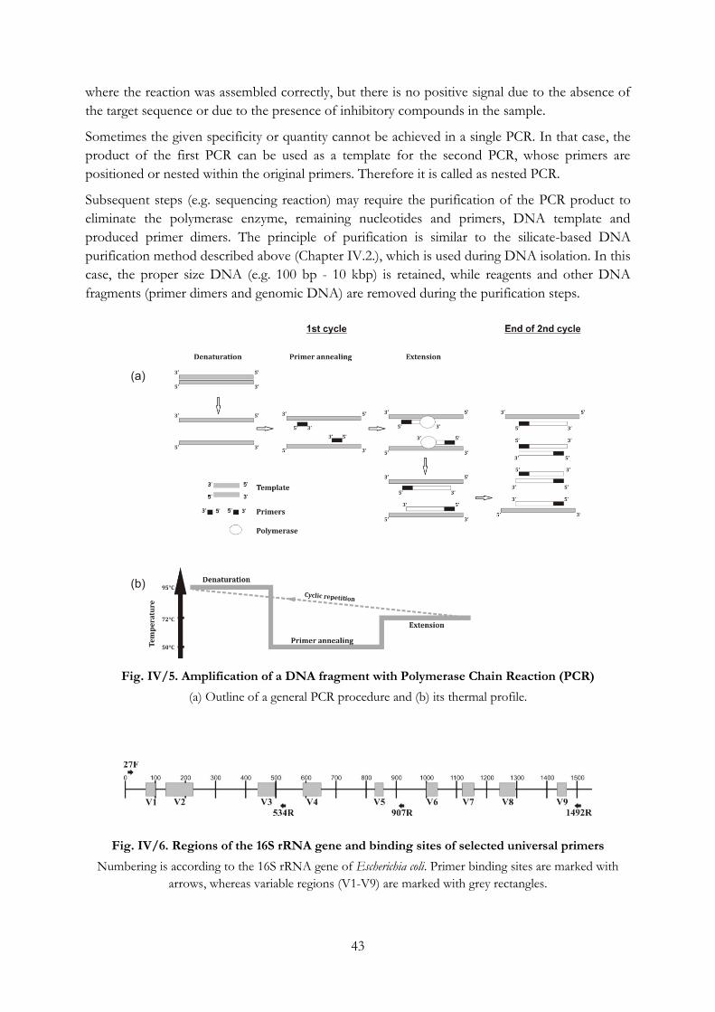
43
where the reaction was assembled correctly, but there is no positive signal due to the absence of
the target sequence or due to the presence of inhibitory compounds in the sample.
Sometimes the given specificity or quantity cannot be achieved in a single PCR. In that case, the
product of the first PCR can be used as a template for the second PCR, whose primers are
positioned or nested within the original primers. Therefore it is called as nested PCR.
Subsequent steps (e.g. sequencing reaction) may require the purification of the PCR product to
eliminate the polymerase enzyme, remaining nucleotides and primers, DNA template and
produced primer dimers. The principle of purification is similar to the silicate-based DNA
purification method described above (Chapter IV.2.), which is used during DNA isolation. In this
case, the proper size DNA (e.g. 100 bp - 10 kbp) is retained, while reagents and other DNA
fragments (primer dimers and genomic DNA) are removed during the purification steps.
Fig. IV/5. Amplification of a DNA fragment with Polymerase Chain Reaction (PCR)
(a) Outline of a general PCR procedure and (b) its thermal profile.
Fig. IV/6. Regions of the 16S rRNA gene and binding sites of selected universal primers
Numbering is according to the 16S rRNA gene of Escherichia coli. Primer binding sites are marked with
arrows, whereas variable regions (V1-V9) are marked with grey rectangles.
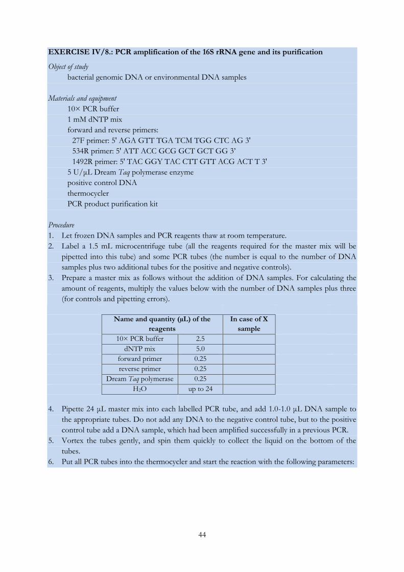
44
EXERCISE IV/8.: PCR amplification of the 16S rRNA gene and its purification
Object of study
bacterial genomic DNA or environmental DNA samples
Materials and equipment
10× PCR buffer
1 mM dNTP mix
forward and reverse primers:
27F primer: 5' AGA GTT TGA TCM TGG CTC AG 3'
534R primer: 5' ATT ACC GCG GCT GCT GG 3’
1492R primer: 5' TAC GGY TAC CTT GTT ACG ACT T 3'
5 U/μL Dream Taq polymerase enzyme
positive control DNA
thermocycler
PCR product purification kit
Procedure
1. Let frozen DNA samples and PCR reagents thaw at room temperature.
2. Label a 1.5 mL microcentrifuge tube (all the reagents required for the master mix will be
pipetted into this tube) and some PCR tubes (the number is equal to the number of DNA
samples plus two additional tubes for the positive and negative controls).
3. Prepare a master mix as follows without the addition of DNA samples. For calculating the
amount of reagents, multiply the values below with the number of DNA samples plus three
(for controls and pipetting errors).
Name and quantity (µL) of the
reagents
In case of X
sample
10× PCR buffer 2.5
dNTP mix 5.0
forward primer 0.25
reverse primer 0.25
Dream Taq polymerase 0.25
H2O up to 24
4. Pipette 24 μL master mix into each labelled PCR tube, and add 1.0-1.0 μL DNA sample to
the appropriate tubes. Do not add any DNA to the negative control tube, but to the positive
control tube add a DNA sample, which had been amplified successfully in a previous PCR.
5. Vortex the tubes gently, and spin them quickly to collect the liquid on the bottom of the
tubes.
6. Put all PCR tubes into the thermocycler and start the reaction with the following parameters:
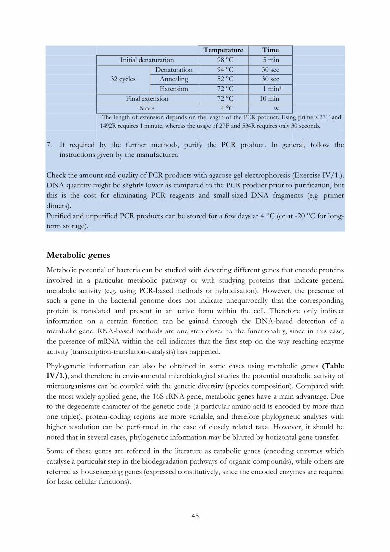
45
Temperature Time
Initial denaturation 98 °C 5 min
32 cycles
Denaturation 94 °C 30 sec
Annealing 52 °C 30 sec
Extension 72 °C 1 min1s
Final extension 72 °C 10 min
Store 4 °C ∞
1The length of extension depends on the length of the PCR product. Using primers 27F and
1492R requires 1 minute, whereas the usage of 27F and 534R requires only 30 seconds.
7. If required by the further methods, purify the PCR product. In general, follow the
instructions given by the manufacturer.
Check the amount and quality of PCR products with agarose gel electrophoresis (Exercise IV/1.).
DNA quantity might be slightly lower as compared to the PCR product prior to purification, but
this is the cost for eliminating PCR reagents and small-sized DNA fragments (e.g. primer
dimers).
Purified and unpurified PCR products can be stored for a few days at 4 °C (or at -20 °C for long-
term storage).
Metabolic genes
Metabolic potential of bacteria can be studied with detecting different genes that encode proteins
involved in a particular metabolic pathway or with studying proteins that indicate general
metabolic activity (e.g. using PCR-based methods or hybridisation). However, the presence of
such a gene in the bacterial genome does not indicate unequivocally that the corresponding
protein is translated and present in an active form within the cell. Therefore only indirect
information on a certain function can be gained through the DNA-based detection of a
metabolic gene. RNA-based methods are one step closer to the functionality, since in this case,
the presence of mRNA within the cell indicates that the first step on the way reaching enzyme
activity (transcription-translation-catalysis) has happened.
Phylogenetic information can also be obtained in some cases using metabolic genes (Table
IV/1.), and therefore in environmental microbiological studies the potential metabolic activity of
microorganisms can be coupled with the genetic diversity (species composition). Compared with
the most widely applied gene, the 16S rRNA gene, metabolic genes have a main advantage. Due
to the degenerate character of the genetic code (a particular amino acid is encoded by more than
one triplet), protein-coding regions are more variable, and therefore phylogenetic analyses with
higher resolution can be performed in the case of closely related taxa. However, it should be
noted that in several cases, phylogenetic information may be blurred by horizontal gene transfer.
Some of these genes are referred in the literature as catabolic genes (encoding enzymes which
catalyse a particular step in the biodegradation pathways of organic compounds), while others are
referred as housekeeping genes (expressed constitutively, since the encoded enzymes are required
for basic cellular functions).
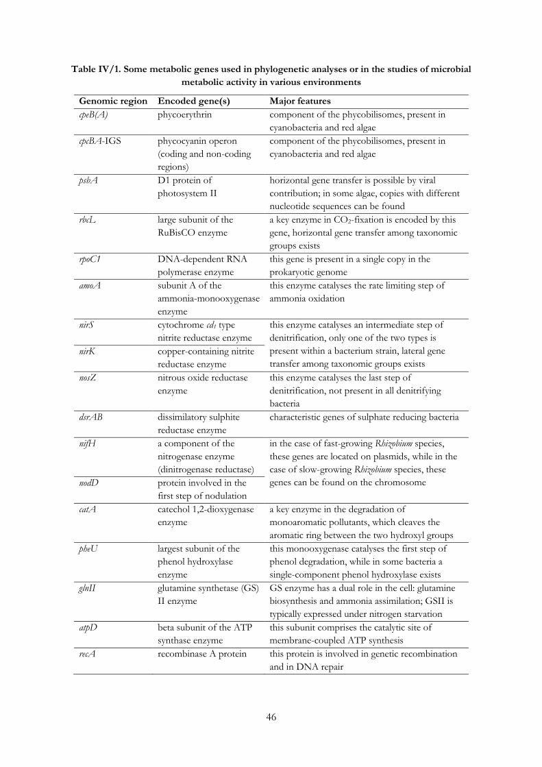
46
Table IV/1. Some metabolic genes used in phylogenetic analyses or in the studies of microbial
metabolic activity in various environments
Genomic region Encoded gene(s) Major features
cpeB(A) phycoerythrin component of the phycobilisomes, present in
cyanobacteria and red algae
cpcBA-IGS phycocyanin operon
(coding and non-coding
regions)
component of the phycobilisomes, present in
cyanobacteria and red algae
psbA D1 protein of
photosystem II
horizontal gene transfer is possible by viral
contribution; in some algae, copies with different
nucleotide sequences can be found
rbcL large subunit of the
RuBisCO enzyme
a key enzyme in CO2-fixation is encoded by this
gene, horizontal gene transfer among taxonomic
groups exists
rpoC1 DNA-dependent RNA
polymerase enzyme
this gene is present in a single copy in the
prokaryotic genome
amoA subunit A of the
ammonia-monooxygenase
enzyme
this enzyme catalyses the rate limiting step of
ammonia oxidation
nirS cytochrome cd1 type
nitrite reductase enzyme
this enzyme catalyses an intermediate step of
denitrification, only one of the two types is
present within a bacterium strain, lateral gene
transfer among taxonomic groups exists
nirK copper-containing nitrite
reductase enzyme
nosZ nitrous oxide reductase
enzyme
this enzyme catalyses the last step of
denitrification, not present in all denitrifying
bacteria
dsrAB dissimilatory sulphite
reductase enzyme
characteristic genes of sulphate reducing bacteria
nifH a component of the
nitrogenase enzyme
(dinitrogenase reductase)
in the case of fast-growing Rhizobium species,
these genes are located on plasmids, while in the
case of slow-growing Rhizobium species, these
genes can be found on the chromosome nodD protein involved in the
first step of nodulation
catA catechol 1,2-dioxygenase
enzyme
a key enzyme in the degradation of
monoaromatic pollutants, which cleaves the
aromatic ring between the two hydroxyl groups
pheU largest subunit of the
phenol hydroxylase
enzyme
this monooxygenase catalyses the first step of
phenol degradation, while in some bacteria a
single-component phenol hydroxylase exists
glnII glutamine synthetase (GS)
II enzyme
GS enzyme has a dual role in the cell: glutamine
biosynthesis and ammonia assimilation; GSII is
typically expressed under nitrogen starvation
atpD beta subunit of the ATP
synthase enzyme
this subunit comprises the catalytic site of
membrane-coupled ATP synthesis
recA recombinase A protein this protein is involved in genetic recombination
and in DNA repair
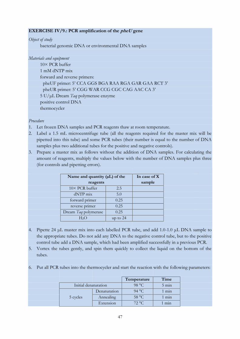
47
EXERCISE IV/9.: PCR amplification of the pheU gene
Object of study
bacterial genomic DNA or environmental DNA samples
Materials and equipment
10× PCR buffer
1 mM dNTP mix
forward and reverse primers:
pheUF primer: 5’ CCA GGS BGA RAA RGA GAR GAA RCT 3’
pheUR primer: 5’ CGG WAR CCG CGC CAG AAC CA 3’
5 U/μL Dream Taq polymerase enzyme
positive control DNA
thermocycler
Procedure
1. Let frozen DNA samples and PCR reagents thaw at room temperature.
2. Label a 1.5 mL microcentrifuge tube (all the reagents required for the master mix will be
pipetted into this tube) and some PCR tubes (their number is equal to the number of DNA
samples plus two additional tubes for the positive and negative controls).
3. Prepare a master mix as follows without the addition of DNA samples. For calculating the
amount of reagents, multiply the values below with the number of DNA samples plus three
(for controls and pipetting errors).
Name and quantity (µL) of the
reagents
In case of X
sample
10× PCR buffer 2.5
dNTP mix 5.0
forward primer 0.25
reverse primer 0.25
Dream Taq polymerase 0.25
H2O up to 24
4. Pipette 24 μL master mix into each labelled PCR tube, and add 1.0-1.0 μL DNA sample to
the appropriate tubes. Do not add any DNA to the negative control tube, but to the positive
control tube add a DNA sample, which had been amplified successfully in a previous PCR.
5. Vortex the tubes gently, and spin them quickly to collect the liquid on the bottom of the
tubes.
6. Put all PCR tubes into the thermocycler and start the reaction with the following parameters:
Temperature Time
Initial denaturation 98 °C 5 min
5 cycles
Denaturation 94 °C 1 min
Annealing 58 °C 1 min
Extension 72 °C 1 min
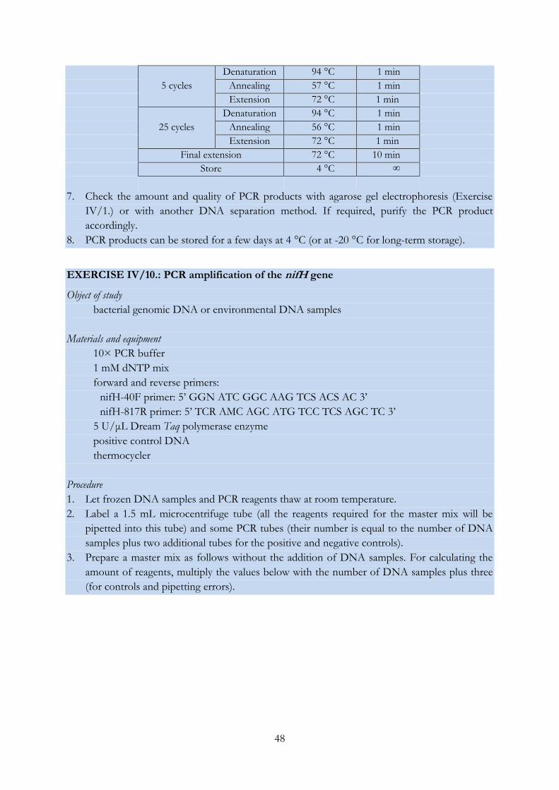
48
5 cycles
Denaturation 94 °C 1 min
Annealing 57 °C 1 min
Extension 72 °C 1 min
25 cycles
Denaturation 94 °C 1 min
Annealing 56 °C 1 min
Extension 72 °C 1 min
Final extension 72 °C 10 min
Store 4 °C ∞
7. Check the amount and quality of PCR products with agarose gel electrophoresis (Exercise
IV/1.) or with another DNA separation method. If required, purify the PCR product
accordingly.
8. PCR products can be stored for a few days at 4 °C (or at -20 °C for long-term storage).
EXERCISE IV/10.: PCR amplification of the nifH gene
Object of study
bacterial genomic DNA or environmental DNA samples
Materials and equipment
10× PCR buffer
1 mM dNTP mix
forward and reverse primers:
nifH-40F primer: 5’ GGN ATC GGC AAG TCS ACS AC 3’
nifH-817R primer: 5’ TCR AMC AGC ATG TCC TCS AGC TC 3’
5 U/μL Dream Taq polymerase enzyme
positive control DNA
thermocycler
Procedure
1. Let frozen DNA samples and PCR reagents thaw at room temperature.
2. Label a 1.5 mL microcentrifuge tube (all the reagents required for the master mix will be
pipetted into this tube) and some PCR tubes (their number is equal to the number of DNA
samples plus two additional tubes for the positive and negative controls).
3. Prepare a master mix as follows without the addition of DNA samples. For calculating the
amount of reagents, multiply the values below with the number of DNA samples plus three
(for controls and pipetting errors).
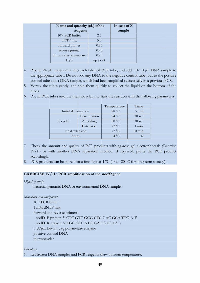
49
Name and quantity (µL) of the
reagents
In case of X
sample
10× PCR buffer 2.5
dNTP mix 5.0
forward primer 0.25
reverse primer 0.25
Dream Taq polymerase 0.25
H2O up to 24
4. Pipette 24 μL master mix into each labelled PCR tube, and add 1.0-1.0 μL DNA sample to
the appropriate tubes. Do not add any DNA to the negative control tube, but to the positive
control tube add a DNA sample, which had been amplified successfully in a previous PCR.
5. Vortex the tubes gently, and spin them quickly to collect the liquid on the bottom of the
tubes.
6. Put all PCR tubes into the thermocycler and start the reaction with the following parameters:
Temperature Time
Initial denaturation 98 °C 5 min
35 cycles
Denaturation 94 °C 30 sec
Annealing 50 °C 30 sec
Extension 72 °C 1 min
Final extension 72 °C 10 min
Store 4 °C ∞
7. Check the amount and quality of PCR products with agarose gel electrophoresis (Exercise
IV/1.) or with another DNA separation method. If required, purify the PCR product
accordingly.
8. PCR products can be stored for a few days at 4 °C (or at -20 °C for long-term storage).
EXERCISE IV/11.: PCR amplification of the nodD gene
Object of study
bacterial genomic DNA or environmental DNA samples
Materials and equipment
10× PCR buffer
1 mM dNTP mix
forward and reverse primers:
nodD1F primer: 5’ CTC GTC GCG CTC GAC GCA TTG A 3’
nodD1R primer: 5’ TGC CCC ATG GAC ATG TA 3’
5 U/μL Dream Taq polymerase enzyme
positive control DNA
thermocycler
Procedure
1. Let frozen DNA samples and PCR reagents thaw at room temperature.
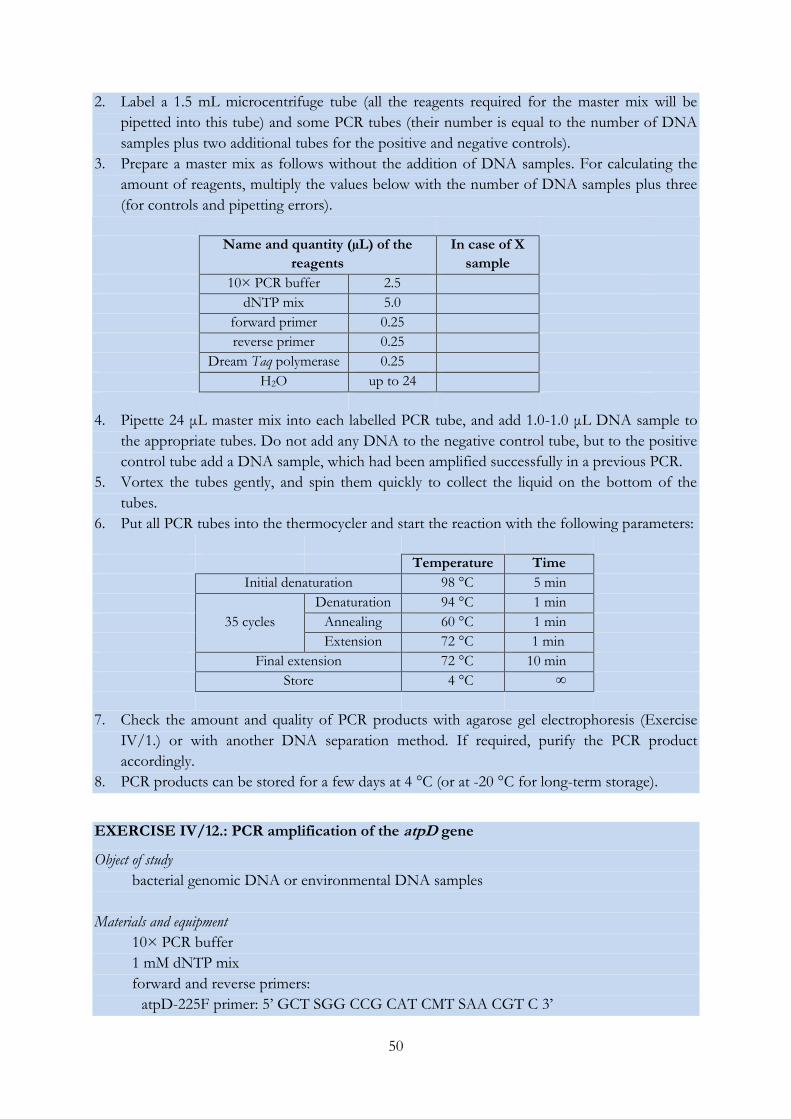
50
2. Label a 1.5 mL microcentrifuge tube (all the reagents required for the master mix will be
pipetted into this tube) and some PCR tubes (their number is equal to the number of DNA
samples plus two additional tubes for the positive and negative controls).
3. Prepare a master mix as follows without the addition of DNA samples. For calculating the
amount of reagents, multiply the values below with the number of DNA samples plus three
(for controls and pipetting errors).
Name and quantity (µL) of the
reagents
In case of X
sample
10× PCR buffer 2.5
dNTP mix 5.0
forward primer 0.25
reverse primer 0.25
Dream Taq polymerase 0.25
H2O up to 24
4. Pipette 24 μL master mix into each labelled PCR tube, and add 1.0-1.0 μL DNA sample to
the appropriate tubes. Do not add any DNA to the negative control tube, but to the positive
control tube add a DNA sample, which had been amplified successfully in a previous PCR.
5. Vortex the tubes gently, and spin them quickly to collect the liquid on the bottom of the
tubes.
6. Put all PCR tubes into the thermocycler and start the reaction with the following parameters:
Temperature Time
Initial denaturation 98 °C 5 min
35 cycles
Denaturation 94 °C 1 min
Annealing 60 °C 1 min
Extension 72 °C 1 min
Final extension 72 °C 10 min
Store 4 °C ∞
7. Check the amount and quality of PCR products with agarose gel electrophoresis (Exercise
IV/1.) or with another DNA separation method. If required, purify the PCR product
accordingly.
8. PCR products can be stored for a few days at 4 °C (or at -20 °C for long-term storage).
EXERCISE IV/12.: PCR amplification of the atpD gene
Object of study
bacterial genomic DNA or environmental DNA samples
Materials and equipment
10× PCR buffer
1 mM dNTP mix
forward and reverse primers:
atpD-225F primer: 5’ GCT SGG CCG CAT CMT SAA CGT C 3’
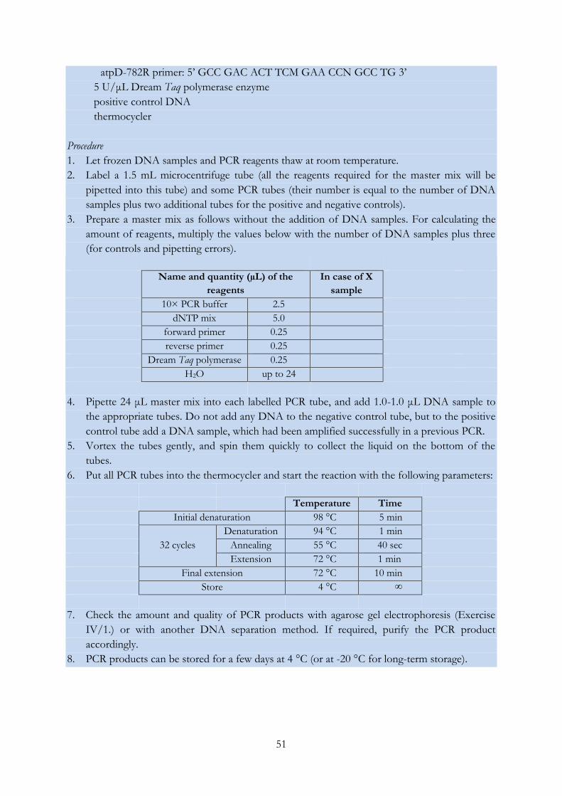
51
atpD-782R primer: 5’ GCC GAC ACT TCM GAA CCN GCC TG 3’
5 U/μL Dream Taq polymerase enzyme
positive control DNA
thermocycler
Procedure
1. Let frozen DNA samples and PCR reagents thaw at room temperature.
2. Label a 1.5 mL microcentrifuge tube (all the reagents required for the master mix will be
pipetted into this tube) and some PCR tubes (their number is equal to the number of DNA
samples plus two additional tubes for the positive and negative controls).
3. Prepare a master mix as follows without the addition of DNA samples. For calculating the
amount of reagents, multiply the values below with the number of DNA samples plus three
(for controls and pipetting errors).
Name and quantity (µL) of the
reagents
In case of X
sample
10× PCR buffer 2.5
dNTP mix 5.0
forward primer 0.25
reverse primer 0.25
Dream Taq polymerase 0.25
H2O up to 24
4. Pipette 24 μL master mix into each labelled PCR tube, and add 1.0-1.0 μL DNA sample to
the appropriate tubes. Do not add any DNA to the negative control tube, but to the positive
control tube add a DNA sample, which had been amplified successfully in a previous PCR.
5. Vortex the tubes gently, and spin them quickly to collect the liquid on the bottom of the
tubes.
6. Put all PCR tubes into the thermocycler and start the reaction with the following parameters:
Temperature Time
Initial denaturation 98 °C 5 min
32 cycles
Denaturation 94 °C 1 min
Annealing 55 °C 40 sec
Extension 72 °C 1 min
Final extension 72 °C 10 min
Store 4 °C ∞
7. Check the amount and quality of PCR products with agarose gel electrophoresis (Exercise
IV/1.) or with another DNA separation method. If required, purify the PCR product
accordingly.
8. PCR products can be stored for a few days at 4 °C (or at -20 °C for long-term storage).
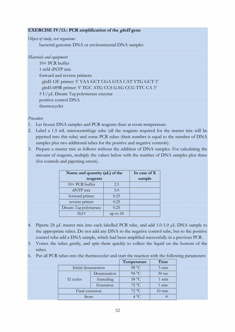
52
EXERCISE IV/13.: PCR amplification of the glnII gene
Object of study, test organisms
bacterial genomic DNA or environmental DNA samples
Materials and equipment
10× PCR buffer
1 mM dNTP mix
forward and reverse primers:
glnII-12F primer: 5’ YAA GCT CGA GTA CAT YTG GCT 3’
glnII-689R primer: 5’ TGC ATG CCS GAG CCG TTC CA 3’
5 U/μL Dream Taq polymerase enzyme
positive control DNA
thermocycler
Procedure
1. Let frozen DNA samples and PCR reagents thaw at room temperature.
2. Label a 1.5 mL microcentrifuge tube (all the reagents required for the master mix will be
pipetted into this tube) and some PCR tubes (their number is equal to the number of DNA
samples plus two additional tubes for the positive and negative controls).
3. Prepare a master mix as follows without the addition of DNA samples. For calculating the
amount of reagents, multiply the values below with the number of DNA samples plus three
(for controls and pipetting errors).
Name and quantity (µL) of the
reagents
In case of X
sample
10× PCR buffer 2.5
dNTP mix 5.0
forward primer 0.25
reverse primer 0.25
Dream Taq polymerase 0.25
H2O up to 24
4. Pipette 24 μL master mix into each labelled PCR tube, and add 1.0-1.0 μL DNA sample to
the appropriate tubes. Do not add any DNA to the negative control tube, but to the positive
control tube add a DNA sample, which had been amplified successfully in a previous PCR.
5. Vortex the tubes gently, and spin them quickly to collect the liquid on the bottom of the
tubes.
6. Put all PCR tubes into the thermocycler and start the reaction with the following parameters:
Temperature Time
Initial denaturation 98 °C 5 min
32 cycles
Denaturation 94 °C 30 sec
Annealing 58 °C 1 min
Extension 72 °C 1 min
Final extension 72 °C 10 min
Store 4 °C ∞
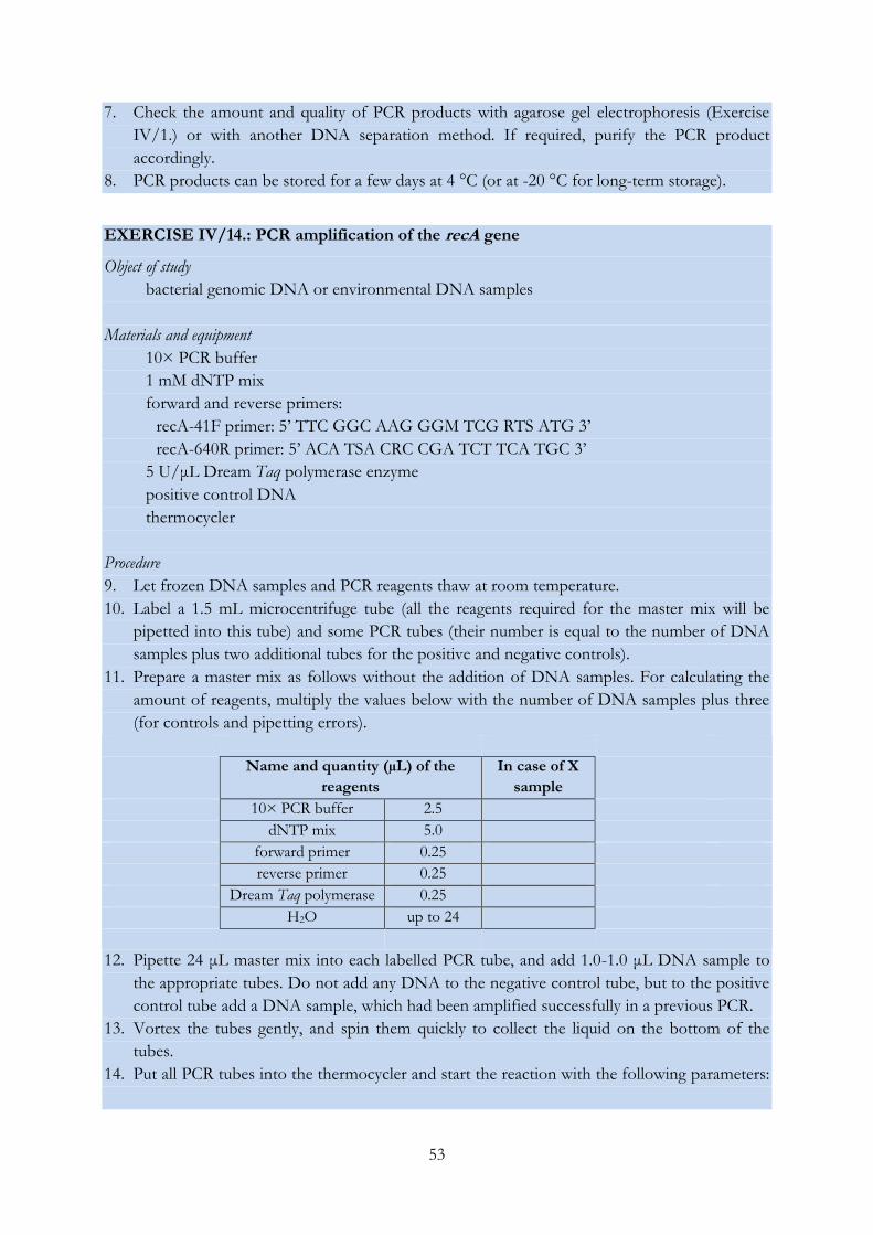
53
7. Check the amount and quality of PCR products with agarose gel electrophoresis (Exercise
IV/1.) or with another DNA separation method. If required, purify the PCR product
accordingly.
8. PCR products can be stored for a few days at 4 °C (or at -20 °C for long-term storage).
EXERCISE IV/14.: PCR amplification of the recA gene
Object of study
bacterial genomic DNA or environmental DNA samples
Materials and equipment
10× PCR buffer
1 mM dNTP mix
forward and reverse primers:
recA-41F primer: 5’ TTC GGC AAG GGM TCG RTS ATG 3’
recA-640R primer: 5’ ACA TSA CRC CGA TCT TCA TGC 3’
5 U/μL Dream Taq polymerase enzyme
positive control DNA
thermocycler
Procedure
9. Let frozen DNA samples and PCR reagents thaw at room temperature.
10. Label a 1.5 mL microcentrifuge tube (all the reagents required for the master mix will be
pipetted into this tube) and some PCR tubes (their number is equal to the number of DNA
samples plus two additional tubes for the positive and negative controls).
11. Prepare a master mix as follows without the addition of DNA samples. For calculating the
amount of reagents, multiply the values below with the number of DNA samples plus three
(for controls and pipetting errors).
Name and quantity (µL) of the
reagents
In case of X
sample
10× PCR buffer 2.5
dNTP mix 5.0
forward primer 0.25
reverse primer 0.25
Dream Taq polymerase 0.25
H2O up to 24
12. Pipette 24 μL master mix into each labelled PCR tube, and add 1.0-1.0 μL DNA sample to
the appropriate tubes. Do not add any DNA to the negative control tube, but to the positive
control tube add a DNA sample, which had been amplified successfully in a previous PCR.
13. Vortex the tubes gently, and spin them quickly to collect the liquid on the bottom of the
tubes.
14. Put all PCR tubes into the thermocycler and start the reaction with the following parameters:
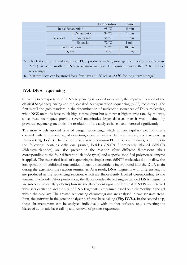
54
Temperature Time
Initial denaturation 98 °C 5 min
32 cycles
Denaturation 94 °C 1 min
Annealing 58 °C 1 min
Extension 72 °C 1 min
Final extension 72 °C 10 min
Store 4 °C ∞
15. Check the amount and quality of PCR products with agarose gel electrophoresis (Exercise
IV/1.) or with another DNA separation method. If required, purify the PCR product
accordingly.
16. PCR products can be stored for a few days at 4 °C (or at -20 °C for long-term storage).
IV.4. DNA sequencing
Currently two major types of DNA sequencing is applied worldwide, the improved version of the
classical Sanger sequencing and the so-called next-generation sequencing (NGS) techniques. The
first is still the gold standard in the determination of nucleotide sequences of DNA molecules,
while NGS methods have much higher throughput but somewhat higher error rate. By the way,
since these techniques provide several magnitudes larger datasets than it was obtained by
previous sequencing methods, the resolution of the analyses have been increased significantly.
The most widely applied type of Sanger sequencing, which applies capillary electrophoresis
coupled with fluorescent signal detection, operates with a chain-terminating cycle sequencing
reaction (Fig. IV/7.). The reaction is similar to a common PCR in several features, but differs in
the following: contains only one primer, besides dNTPs fluorescently labelled ddNTPs
(dideoxynucleotides) are also present in the reaction (four different fluorescent labels
corresponding to the four different nucleotide types) and a special modified polymerase enzyme
is applied. The theoretical basis of sequencing is simple: since ddNTP molecules do not allow the
incorporation of additional nucleotides, if such a nucleotide is incorporated into the DNA chain
during the extension, the reaction terminates. As a result, DNA fragments with different lengths
are produced in the sequencing reaction, which are fluorescently labelled corresponding to the
terminal nucleotide. After purification, the fluorescently-labelled single-stranded DNA fragments
are subjected to capillary electrophoresis: the fluorescent signals of terminal ddNTPs are detected
with laser excitation and the size of DNA fragments is measured based on their motility in the gel
within the capillary. The created sequencing chromatograms are analysed in two separate steps.
First, the software in the genetic analyser performs base-calling (Fig. IV/8.). In the second step,
these chromatograms can be analysed individually with another software (e.g. correcting the
biases of automatic base-calling and removal of primer sequences).
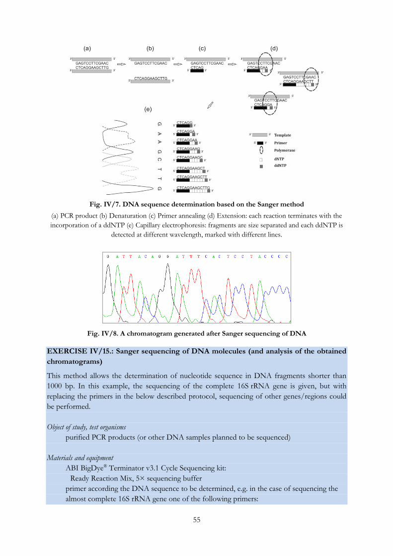
55
Fig. IV/7. DNA sequence determination based on the Sanger method
(a) PCR product (b) Denaturation (c) Primer annealing (d) Extension: each reaction terminates with the
incorporation of a ddNTP (e) Capillary electrophoresis: fragments are size separated and each ddNTP is
detected at different wavelength, marked with different lines.
Fig. IV/8. A chromatogram generated after Sanger sequencing of DNA
EXERCISE IV/15.: Sanger sequencing of DNA molecules (and analysis of the obtained
chromatograms)
This method allows the determination of nucleotide sequence in DNA fragments shorter than
1000 bp. In this example, the sequencing of the complete 16S rRNA gene is given, but with
replacing the primers in the below described protocol, sequencing of other genes/regions could
be performed.
Object of study, test organisms
purified PCR products (or other DNA samples planned to be sequenced)
Materials and equipment
ABI BigDye® Terminator v3.1 Cycle Sequencing kit:
Ready Reaction Mix, 5× sequencing buffer
primer according the DNA sequence to be determined, e.g. in the case of sequencing the
almost complete 16S rRNA gene one of the following primers:
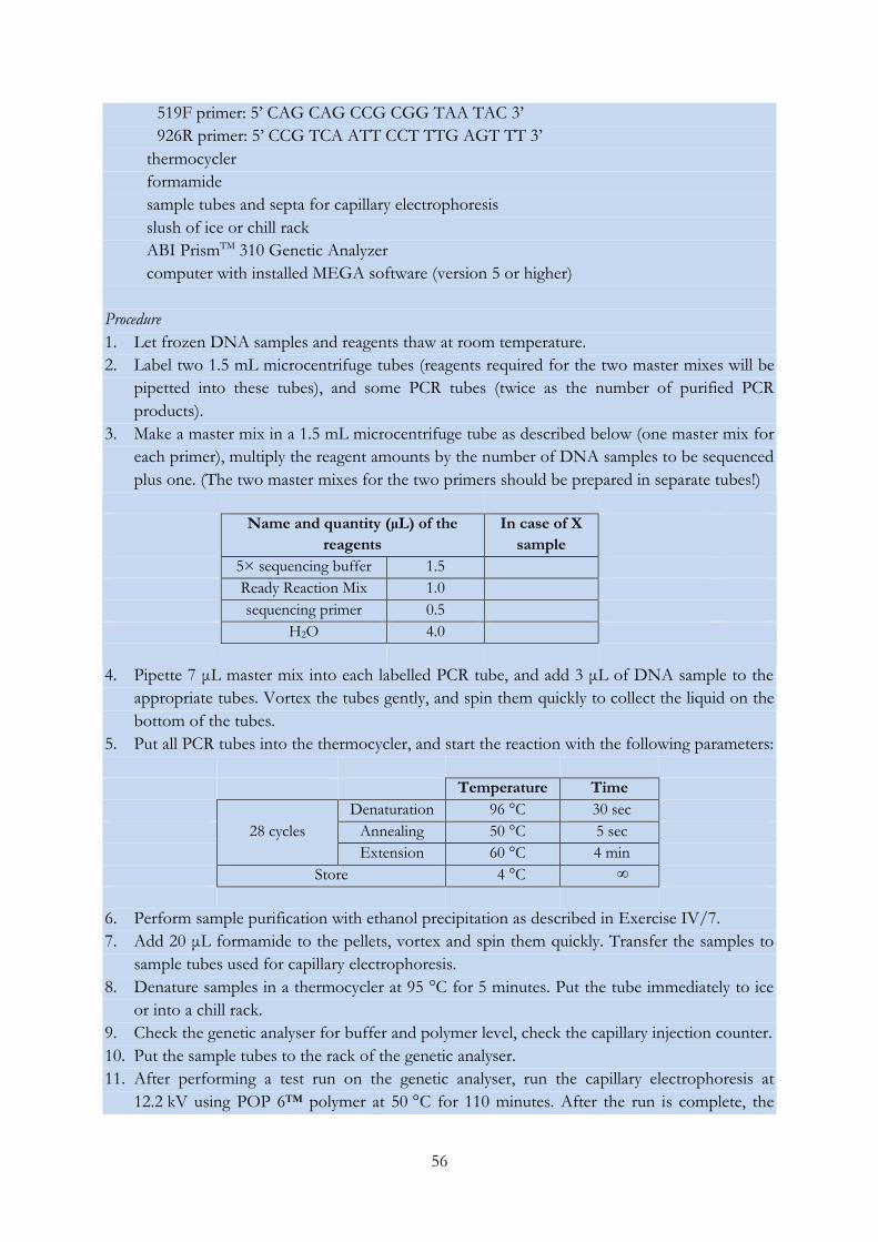
56
519F primer: 5’ CAG CAG CCG CGG TAA TAC 3’
926R primer: 5’ CCG TCA ATT CCT TTG AGT TT 3’
thermocycler
formamide
sample tubes and septa for capillary electrophoresis
slush of ice or chill rack
ABI PrismTM 310 Genetic Analyzer
computer with installed MEGA software (version 5 or higher)
Procedure
1. Let frozen DNA samples and reagents thaw at room temperature.
2. Label two 1.5 mL microcentrifuge tubes (reagents required for the two master mixes will be
pipetted into these tubes), and some PCR tubes (twice as the number of purified PCR
products).
3. Make a master mix in a 1.5 mL microcentrifuge tube as described below (one master mix for
each primer), multiply the reagent amounts by the number of DNA samples to be sequenced
plus one. (The two master mixes for the two primers should be prepared in separate tubes!)
Name and quantity (µL) of the
reagents
In case of X
sample
5× sequencing buffer 1.5
Ready Reaction Mix 1.0
sequencing primer 0.5
H2O 4.0
4. Pipette 7 μL master mix into each labelled PCR tube, and add 3 μL of DNA sample to the
appropriate tubes. Vortex the tubes gently, and spin them quickly to collect the liquid on the
bottom of the tubes.
5. Put all PCR tubes into the thermocycler, and start the reaction with the following parameters:
Temperature Time
28 cycles
Denaturation 96 °C 30 sec
Annealing 50 °C 5 sec
Extension 60 °C 4 min
Store 4 °C ∞
6. Perform sample purification with ethanol precipitation as described in Exercise IV/7.
7. Add 20 μL formamide to the pellets, vortex and spin them quickly. Transfer the samples to
sample tubes used for capillary electrophoresis.
8. Denature samples in a thermocycler at 95 °C for 5 minutes. Put the tube immediately to ice
or into a chill rack.
9. Check the genetic analyser for buffer and polymer level, check the capillary injection counter.
10. Put the sample tubes to the rack of the genetic analyser.
11. After performing a test run on the genetic analyser, run the capillary electrophoresis at
12.2 kV using POP 6™ polymer at 50 °C for 110 minutes. After the run is complete, the
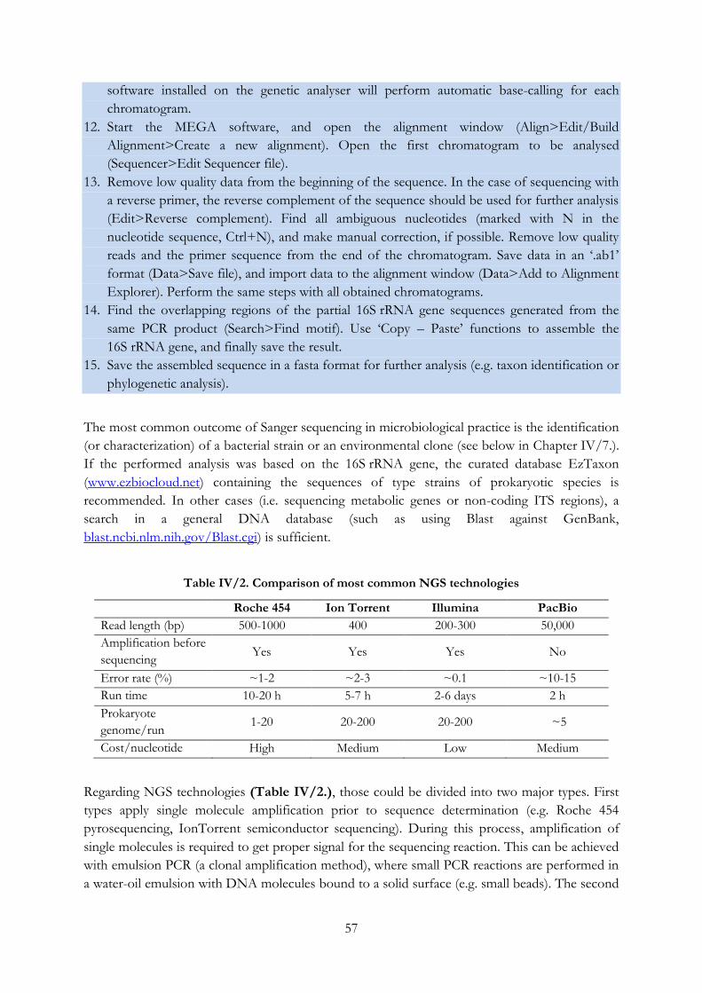
57
software installed on the genetic analyser will perform automatic base-calling for each
chromatogram.
12. Start the MEGA software, and open the alignment window (Align>Edit/Build
Alignment>Create a new alignment). Open the first chromatogram to be analysed
(Sequencer>Edit Sequencer file).
13. Remove low quality data from the beginning of the sequence. In the case of sequencing with
a reverse primer, the reverse complement of the sequence should be used for further analysis
(Edit>Reverse complement). Find all ambiguous nucleotides (marked with N in the
nucleotide sequence, Ctrl+N), and make manual correction, if possible. Remove low quality
reads and the primer sequence from the end of the chromatogram. Save data in an ‘.ab1’
format (Data>Save file), and import data to the alignment window (Data>Add to Alignment
Explorer). Perform the same steps with all obtained chromatograms.
14. Find the overlapping regions of the partial 16S rRNA gene sequences generated from the
same PCR product (Search>Find motif). Use ‘Copy – Paste’ functions to assemble the
16S rRNA gene, and finally save the result.
15. Save the assembled sequence in a fasta format for further analysis (e.g. taxon identification or
phylogenetic analysis).
The most common outcome of Sanger sequencing in microbiological practice is the identification
(or characterization) of a bacterial strain or an environmental clone (see below in Chapter IV/7.).
If the performed analysis was based on the 16S rRNA gene, the curated database EzTaxon
(www.ezbiocloud.net) containing the sequences of type strains of prokaryotic species is
recommended. In other cases (i.e. sequencing metabolic genes or non-coding ITS regions), a
search in a general DNA database (such as using Blast against GenBank,
blast.ncbi.nlm.nih.gov/Blast.cgi) is sufficient.
Table IV/2. Comparison of most common NGS technologies
Roche 454 Ion Torrent Illumina PacBio
Read length (bp) 500-1000 400 200-300 50,000
Amplification before
sequencing Yes Yes Yes No
Error rate (%) ~1-2 ~2-3 ~0.1 ~10-15
Run time 10-20 h 5-7 h 2-6 days 2 h
Prokaryote
genome/run 1-20 20-200 20-200 ~5
Cost/nucleotide High Medium Low Medium
Regarding NGS technologies (Table IV/2.), those could be divided into two major types. First
types apply single molecule amplification prior to sequence determination (e.g. Roche 454
pyrosequencing, IonTorrent semiconductor sequencing). During this process, amplification of
single molecules is required to get proper signal for the sequencing reaction. This can be achieved
with emulsion PCR (a clonal amplification method), where small PCR reactions are performed in
a water-oil emulsion with DNA molecules bound to a solid surface (e.g. small beads). The second
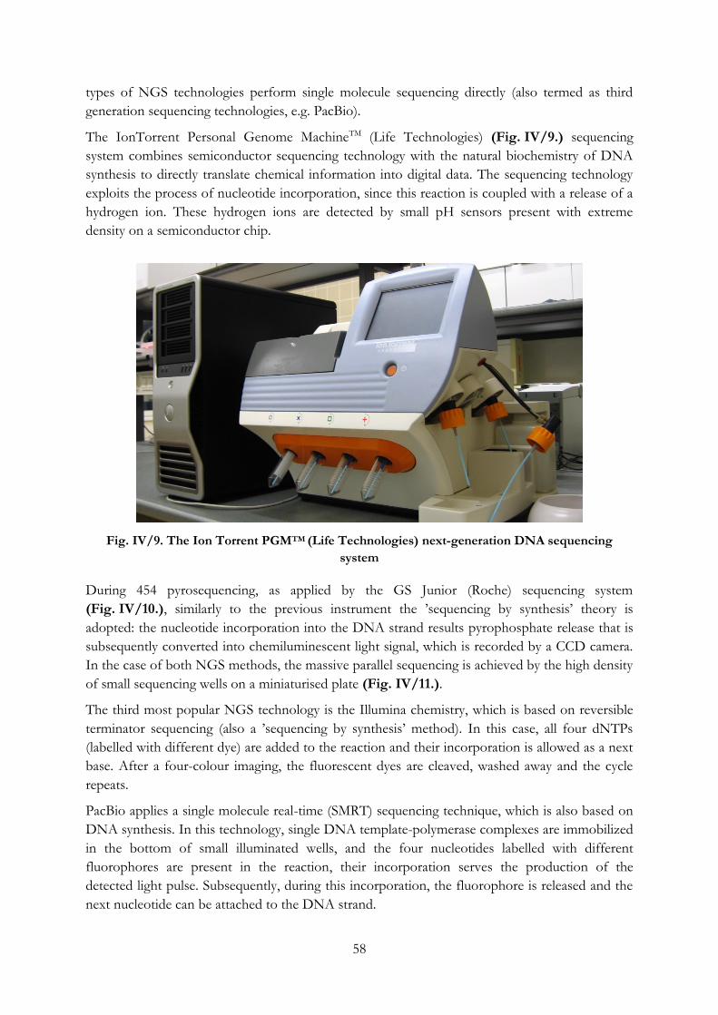
58
types of NGS technologies perform single molecule sequencing directly (also termed as third
generation sequencing technologies, e.g. PacBio).
The IonTorrent Personal Genome MachineTM (Life Technologies) (Fig. IV/9.) sequencing
system combines semiconductor sequencing technology with the natural biochemistry of DNA
synthesis to directly translate chemical information into digital data. The sequencing technology
exploits the process of nucleotide incorporation, since this reaction is coupled with a release of a
hydrogen ion. These hydrogen ions are detected by small pH sensors present with extreme
density on a semiconductor chip.
Fig. IV/9. The Ion Torrent PGMTM (Life Technologies) next-generation DNA sequencing
system
During 454 pyrosequencing, as applied by the GS Junior (Roche) sequencing system
(Fig. IV/10.), similarly to the previous instrument the ’sequencing by synthesis’ theory is
adopted: the nucleotide incorporation into the DNA strand results pyrophosphate release that is
subsequently converted into chemiluminescent light signal, which is recorded by a CCD camera.
In the case of both NGS methods, the massive parallel sequencing is achieved by the high density
of small sequencing wells on a miniaturised plate (Fig. IV/11.).
The third most popular NGS technology is the Illumina chemistry, which is based on reversible
terminator sequencing (also a ’sequencing by synthesis’ method). In this case, all four dNTPs
(labelled with different dye) are added to the reaction and their incorporation is allowed as a next
base. After a four-colour imaging, the fluorescent dyes are cleaved, washed away and the cycle
repeats.
PacBio applies a single molecule real-time (SMRT) sequencing technique, which is also based on
DNA synthesis. In this technology, single DNA template-polymerase complexes are immobilized
in the bottom of small illuminated wells, and the four nucleotides labelled with different
fluorophores are present in the reaction, their incorporation serves the production of the
detected light pulse. Subsequently, during this incorporation, the fluorophore is released and the
next nucleotide can be attached to the DNA strand.
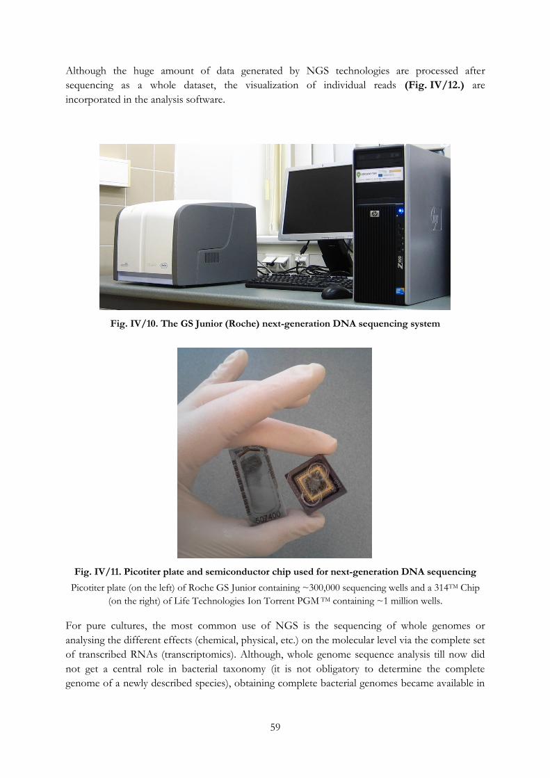
59
Although the huge amount of data generated by NGS technologies are processed after
sequencing as a whole dataset, the visualization of individual reads (Fig. IV/12.) are
incorporated in the analysis software.
Fig. IV/10. The GS Junior (Roche) next-generation DNA sequencing system
Fig. IV/11. Picotiter plate and semiconductor chip used for next-generation DNA sequencing
Picotiter plate (on the left) of Roche GS Junior containing ~300,000 sequencing wells and a 314TM Chip
(on the right) of Life Technologies Ion Torrent PGM TM containing ~1 million wells.
For pure cultures, the most common use of NGS is the sequencing of whole genomes or
analysing the different effects (chemical, physical, etc.) on the molecular level via the complete set
of transcribed RNAs (transcriptomics). Although, whole genome sequence analysis till now did
not get a central role in bacterial taxonomy (it is not obligatory to determine the complete
genome of a newly described species), obtaining complete bacterial genomes became available in
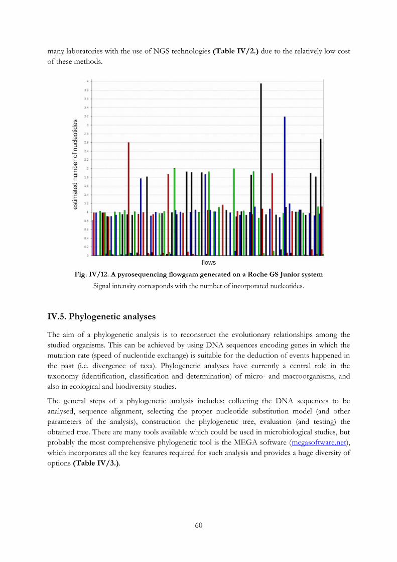
60
many laboratories with the use of NGS technologies (Table IV/2.) due to the relatively low cost
of these methods.
Fig. IV/12. A pyrosequencing flowgram generated on a Roche GS Junior system
Signal intensity corresponds with the number of incorporated nucleotides.
IV.5. Phylogenetic analyses
The aim of a phylogenetic analysis is to reconstruct the evolutionary relationships among the
studied organisms. This can be achieved by using DNA sequences encoding genes in which the
mutation rate (speed of nucleotide exchange) is suitable for the deduction of events happened in
the past (i.e. divergence of taxa). Phylogenetic analyses have currently a central role in the
taxonomy (identification, classification and determination) of micro- and macroorganisms, and
also in ecological and biodiversity studies.
The general steps of a phylogenetic analysis includes: collecting the DNA sequences to be
analysed, sequence alignment, selecting the proper nucleotide substitution model (and other
parameters of the analysis), construction the phylogenetic tree, evaluation (and testing) the
obtained tree. There are many tools available which could be used in microbiological studies, but
probably the most comprehensive phylogenetic tool is the MEGA software (megasoftware.net),
which incorporates all the key features required for such analysis and provides a huge diversity of
options (Table IV/3.).
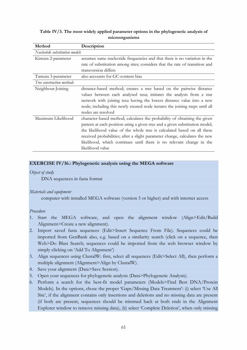
61
Table IV/3. The most widely applied parameter options in the phylogenetic analysis of
microorganisms
Method Description
Nucleotide substitution models
Kimura 2-parameter assumes same nucleotide frequencies and that there is no variation in the
rate of substitution among sites; considers that the rate of transition and
transversion differs
Tamura 3-parameter also accounts for GC-content bias
Tree construction methods
Neighbour-Joining distance-based method; creates a tree based on the pairwise distance
values between each analysed taxa; initiates the analysis from a star
network with joining taxa having the lowest distance value into a new
node; including this newly created node iterates the joining steps until all
nodes are resolved
Maximum Likelihood character-based method; calculates the probability of obtaining the given
pattern at each position using a given tree and a given substitution model;
the likelihood value of the whole tree is calculated based on all these
received probabilities; after a slight parameter change, calculates the new
likelihood, which continues until there is no relevant change in the
likelihood value
EXERCISE IV/16.: Phylogenetic analysis using the MEGA software
Object of study
DNA sequences in fasta format
Materials and equipment
computer with installed MEGA software (version 5 or higher) and with internet access
Procedure
1. Start the MEGA software, and open the alignment window (Align>Edit/Build
Alignment>Create a new alignment).
2. Import saved fasta sequences (Edit>Insert Sequence From File). Sequences could be
imported from GenBank also, e.g. based on a similarity search (click on a sequence, then
Web>Do Blast Search; sequences could be imported from the web browser window by
simply clicking on ‘Add To Alignment’)
3. Align sequences using ClustalW: first, select all sequences (Edit>Select All), then perform a
multiple alignment (Alignment>Align by ClustalW).
4. Save your alignment (Data>Save Session).
5. Open your sequences for phylogenetic analysis (Data>Phylogenetic Analysis).
6. Perform a search for the best-fit model parameters (Models>Find Best DNA/Protein
Models). In the options, chose the proper ‘Gaps/Missing Data Treatment’: (i) select ‘Use All
Site’, if the alignment contains only insertions and deletions and no missing data are present
(if both are present, sequences should be trimmed back at both ends in the Alignment
Explorer window to remove missing data), (ii) select ‘Complete Deletion’, when only missing
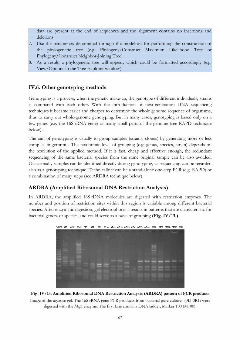
62
data are present at the end of sequences and the alignment contains no insertions and
deletions.
7. Use the parameters determined through the modeltest for performing the construction of
the phylogenetic tree (e.g. Phylogeny/Construct Maximum Likelihood Tree or
Phylogeny/Construct Neighbor-Joining Tree).
8. As a result, a phylogenetic tree will appear, which could be formatted accordingly (e.g.
View/Options in the Tree Explorer window).
IV.6. Other genotyping methods
Genotyping is a process, when the genetic make-up, the genotype of different individuals, strains
is compared with each other. With the introduction of next-generation DNA sequencing
techniques it became easier and cheaper to determine the whole genome sequence of organisms,
thus to carry out whole-genome genotyping. But in many cases, genotyping is based only on a
few genes (e.g. the 16S rRNA gene) or many small parts of the genome (see RAPD technique
below).
The aim of genotyping is usually to group samples (strains, clones) by generating more or less
complex fingerprints. The taxonomic level of grouping (e.g. genus, species, strain) depends on
the resolution of the applied method. If it is fast, cheap and effective enough, the redundant
sequencing of the same bacterial species from the same original sample can be also avoided.
Occasionally samples can be identified directly during genotyping, as sequencing can be regarded
also as a genotyping technique. Technically it can be a stand-alone one-step PCR (e.g. RAPD) or
a combination of many steps (see ARDRA technique below).
ARDRA (Amplified Ribosomal DNA Restriction Analysis)
In ARDRA, the amplified 16S rDNA molecules are digested with restriction enzymes. The
number and position of restriction sites within this region is variable among different bacterial
species. After enzymatic digestion, gel electrophoresis results in patterns that are characteristic for
bacterial genera or species, and could serve as a basis of grouping (Fig. IV/13.).
Fig. IV/13. Amplified Ribosomal DNA Restriction Analysis (ARDRA) pattern of PCR products
Image of the agarose gel. The 16S rRNA gene PCR products from bacterial pure cultures (0I3-0R1) were
digested with the MspI enzyme. The first lane contains DNA ladder, Marker 100 (M100).
63
The patterns are determined only by the position of the restriction sites, and it does not account
for sequence variations outside the recognition positions. Hence it might occur that sequences
without closer relation end up in the same ARDRA group. This bias can be reduced by the
application of more restriction enzymes. During enzymatic digestion, many smaller DNA
fragments are produced, whose separation requires higher resolution than in the case of normal
PCR products. This could be achieved by increasing the electrophoresis time and gel
concentration, and lowering the voltage applied for electrophoresis (see Chapter IV/1).
EXERCISE IV/17.: Restriction digestion of PCR products and pattern analysis
Grouping samples based on the restriction patterns of their PCR products
Object of study
PCR products (e.g. 16S rRNA gene)
Materials and equipment
10× buffer of restriction enzymes
restriction enzymes
water bath
computers with adequate software
Procedure
1. Let frozen PCR products and enzyme buffers thaw at room temperature.
2. Label a 1.5 mL microcentrifuge tube (all the reagents required for the master mix will be
pipetted into this tube) and some 0.6 mL microcentrifuge tubes (the number is equal to the
number of PCR products).
3. Prepare a master mix as follows without the addition of PCR products. For calculating the
amount of reagents, multiply the values below with the number of samples plus one (for
pipetting errors).
Name and quantity (µL) of the
reagents
In case of X
sample
10× enzyme buffer 2.0
enzyme (10 U/µL) 0.15
H2O 9.85
4. Pipette 12 μL master mix into each labelled 0.6 mL microcentrifuge tube, and add 8-8 μL
PCR product to the appropriate tubes.
5. Vortex the tubes gently, and spin them quickly to collect the liquid on the bottom of the
tubes.
6. Incubate the samples in a water bath at the given temperature for 3 hours.
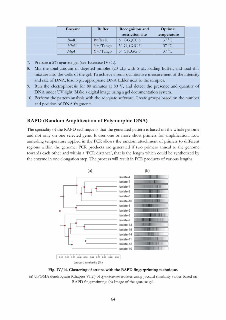
64
Enzyme Buffer Recognition and
restriction site
Optimal
temperature
BsuRI Buffer R 5’ GG↓CC 3’ 37 °C
Hin6I Y+/Tango 5’ G↓CGC 3’ 37 °C
MspI Y+/Tango 5’ C↓CGG 3’ 37 °C
7. Prepare a 2% agarose gel (see Exercise IV/1.).
8. Mix the total amount of digested samples (20 μL) with 5 μL loading buffer, and load this
mixture into the wells of the gel. To achieve a semi-quantitative measurement of the intensity
and size of DNA, load 5 μL appropriate DNA ladder next to the samples.
9. Run the electrophoresis for 80 minutes at 80 V, and detect the presence and quantity of
DNA under UV light. Make a digital image using a gel documentation system.
10. Perform the pattern analysis with the adequate software. Create groups based on the number
and position of DNA fragments.
RAPD (Random Amplification of Polymorphic DNA)
The speciality of the RAPD technique is that the generated pattern is based on the whole genome
and not only on one selected gene. It uses one or more short primers for amplification. Low
annealing temperature applied in the PCR allows the random attachment of primers to different
regions within the genome. PCR products are generated if two primers anneal to the genome
towards each other and within a ‘PCR distance’, that is the length which could be synthetized by
the enzyme in one elongation step. The process will result in PCR products of various lengths.
Fig. IV/14. Clustering of strains with the RAPD fingerprinting technique.
(a) UPGMA dendrogram (Chapter VI.2.) of Synechococcus isolates using Jaccard similarity values based on
RAPD fingerprinting. (b) Image of the agarose gel.
65
The prerequisite of a RAPD analysis is an intact genome, therefore such a DNA extraction
procedure must be chosen that does not significantly fragment genomic DNA (e.g. extraction
based on enzymatic lysis). To achieve the appropriate result, PCR should be performed in three
replicates, since some intra-sample variability may be observed due to the random annealing of
primers to the genomic DNA. After the electrophoresis of the PCR products, dendrogram can
be constructed from the resulting patterns using an image and data analysis software
(Fig. IV/14.).
EXERCISE IV/18.: Distinguishing bacterial strains using the RAPD fingerprinting
technique
Object of study
bacterial genomic DNA
Materials and equipment
10× PCR buffer
1 mM dNTP mix
M13 primer: 5' GAG GGT GGC GGT TCT 3'
5 U/μL Dream Taq polymerase enzyme
positive control DNA
thermocycler
computers with adequate software
Procedure
1. Let frozen DNA samples and PCR reagents thaw at room temperature.
2. Label a 1.5 mL microcentrifuge tube (all the reagents required for the master mix will be
pipetted into this tube) and some PCR tubes (the number is equal to the number of DNA
samples plus two additional tubes for the positive and negative controls).
3. Prepare a master mix as follows without the addition of DNA samples. For calculating the
amount of reagents, multiply the values below with the number of DNA samples plus three
(for controls and pipetting errors).
Name and quantity (µL) of the
reagents
In case of X
sample
10× PCR buffer 2.5
dNTP mix 6.0
M13 primer 2.0
Dream Taq polymerase 0.25
H2O up to 24
4. Pipette 24 μL master mix into each labelled PCR tube, and add 1.0-1.0 μL DNA sample to
the appropriate tubes. Do not add any DNA to the negative control tube, but to the positive
control tube add a DNA sample, which had been amplified successfully in a previous PCR.
5. Vortex the tubes gently, and spin them quickly to collect the liquid on the bottom of the
tubes.
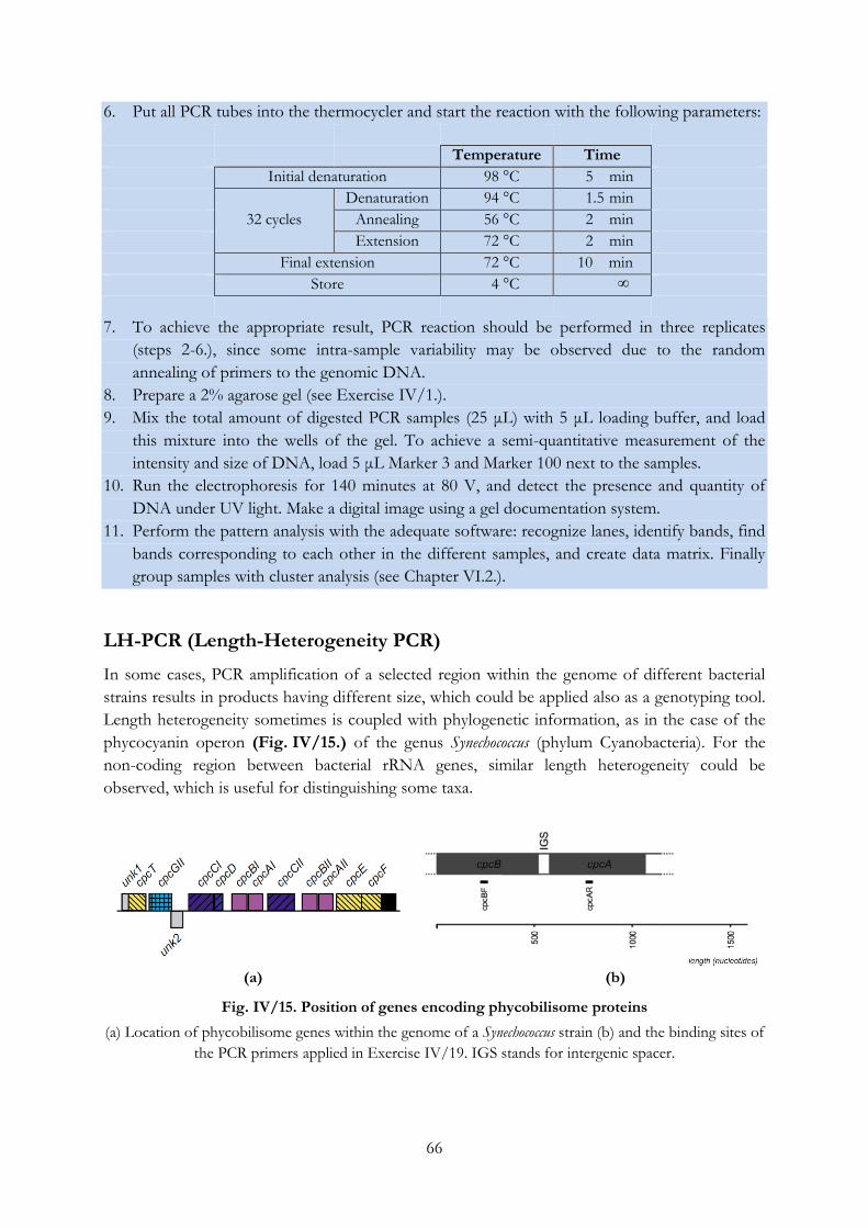
66
6. Put all PCR tubes into the thermocycler and start the reaction with the following parameters:
Temperature Time
Initial denaturation 98 °C 5 min
32 cycles
Denaturation 94 °C 1.5 min
Annealing 56 °C 2 min
Extension 72 °C 2 min
Final extension 72 °C 10 min
Store 4 °C ∞
7. To achieve the appropriate result, PCR reaction should be performed in three replicates
(steps 2-6.), since some intra-sample variability may be observed due to the random
annealing of primers to the genomic DNA.
8. Prepare a 2% agarose gel (see Exercise IV/1.).
9. Mix the total amount of digested PCR samples (25 μL) with 5 μL loading buffer, and load
this mixture into the wells of the gel. To achieve a semi-quantitative measurement of the
intensity and size of DNA, load 5 μL Marker 3 and Marker 100 next to the samples.
10. Run the electrophoresis for 140 minutes at 80 V, and detect the presence and quantity of
DNA under UV light. Make a digital image using a gel documentation system.
11. Perform the pattern analysis with the adequate software: recognize lanes, identify bands, find
bands corresponding to each other in the different samples, and create data matrix. Finally
group samples with cluster analysis (see Chapter VI.2.).
LH-PCR (Length-Heterogeneity PCR)
In some cases, PCR amplification of a selected region within the genome of different bacterial
strains results in products having different size, which could be applied also as a genotyping tool.
Length heterogeneity sometimes is coupled with phylogenetic information, as in the case of the
phycocyanin operon (Fig. IV/15.) of the genus Synechococcus (phylum Cyanobacteria). For the
non-coding region between bacterial rRNA genes, similar length heterogeneity could be
observed, which is useful for distinguishing some taxa.
(a) (b)
Fig. IV/15. Position of genes encoding phycobilisome proteins
(a) Location of phycobilisome genes within the genome of a Synechococcus strain (b) and the binding sites of
the PCR primers applied in Exercise IV/19. IGS stands for intergenic spacer.
67
EXERCISE IV/19.: Genetic characterization of Synechococcus isolates with LH-PCR
Prepare phycocianin operon LH-PCR from DNA isolated from Synechococcus isolates and/or from
lake water samples. The expected size of the PCR product will be determined for different
Synechococcus groups in silico using computational data analysis. Subsequently, the identity of the
unknown isolates and environmental samples will be determined based on the length of the
obtained PCR product.
Object of study
DNA from Synechococcus isolates and lake water samples
Materials and equipment
10× PCR buffer
1 mM dNTP mix
forward and reverse primers:
cpcBF primer: 5' TAG TGT AAA ACG ACG GCC AGT TGY YTK
CGC GAC ATG GA 3'
cpcAR primer: 5' TAG CAG GAA ACA GCT ATG ACG TGG TGT
ARG GGA AYT T 3'
5 U/μL Dream Taq polymerase enzyme
positive control DNA
thermocycler
computer with internet connection
Procedure
1. Let frozen DNA samples and PCR reagents thaw at room temperature.
2. Label a 1.5 mL microcentrifuge tube (all the reagents required for the master mix will be
pipetted into this tube) and some PCR tubes (the number is equal to the number of DNA
samples plus two additional tubes for the positive and negative controls).
3. Prepare a master mix as follows without the addition of DNA samples. For calculating the
amount of reagents, multiply the values below with the number of DNA samples plus three
(for controls and pipetting errors).
Name and quantity (µL) of the
reagents
In case of X
sample
10× PCR buffer 2.5
dNTP mix 5.0
forward primer 0.25
reverse primer 0.25
Dream Taq polymerase 0.25
H2O up to 24
4. Pipette 24 μL master mix into each labelled PCR tube, and add 1.0-1.0 μL DNA sample to
the appropriate tubes. Do not add any DNA to the negative control tube, but to the positive
control tube add a DNA sample, which had been amplified successfully in a previous PCR.
68
5. Vortex the tubes gently, and spin them quickly to collect the liquid on the bottom of the
tubes.
6. Put all PCR tubes into the thermocycler and start the reaction with the following parameters:
Temperature Time
Initial denaturation 98 °C 5 min
32 cycles
Denaturation 94 °C 45 sec
Annealing 45 °C 45 sec
Extension 72 °C 45 sec
Final extension 72 °C 10 min
Store 4 °C ∞
7. Prepare 1 % agarose gel (see Exercise IV/1.), and check the amount and quality of PCR
products in the same way as for general PCR samples.
8. If there are visible PCR products, perform the electrophoresis in a 2% agarose gel to get
better separation of the DNA.
9. Mix the total amount of PCR products (25 μL) with 5 μL loading buffer, and load this
mixture into the wells of the gel. To achieve a semi-quantitative measurement of the intensity
and size of DNA, load 5 μL Maker 100 next to the samples.
10. Run the electrophoresis for 140 minutes at 80 V, and detect the presence and quantity of
DNA under UV light. Make a digital image using a gel documentation system.
11. Calculate the expected size of PCR products of the following reference genotypes. First, find
primer binding sites in the genome of Synechococcus sp. CC9605 (GenBank Acc. No.
NC_007516) and make calculation for the size of the in silico PCR product. Identify and
calculate the size of the overhanging region (which does not contain the IGS) of this virtual
PCR product. Fill the following table with IGS length data retrieved from GenBank in the
case of all reference isolates. Calculate the expected size of cpcBA-IGS PCR products.
Phylogenetic
group Isolate Acc. No. Origin
IGS length (bp)
Length of PCR
product (bp)
A
LS0590 DQ526403 Lake Superior, USA
ACT 1025 HQ859453 Lake Fertő, Austria
ACT 9801 GQ888571 Lake Balaton, Hungary
ACT 9804 GQ888574 Lake Balaton, Hungary
B
BO8807 AY224202 Lake Constance, Europe
PS725 AF223446 Lake Kasumigaura, Japan
MW4C3 AY151213 Mondsee, Austria
MW74D3 AY151220 Hallstattersee, Austria
ACT 9807 GQ888576 Lake Balaton, Hungary
MI0507A FJ763790 Lake Mikolajske, Poland
C
PS684 AF223454 Lake Abashiri, Japan
BE0807F FJ763817 Lake Beldany, Poland
D
PS673 AF223434 Lake Harutori, Japan
PS678 AF223441 Lake Kojima, Japan
M
PS724 AF223436 Lake Tsukui, Japan
MA0607I FJ763810 Lake Majcz, Poland
MA0607J FJ763811 Lake Majcz, Poland
69
12. Calculate the expected size of PCR products for each phylogenetic group. Finally, try to
identify the unknown isolates (and the composition of environmental samples) based on the
size-distribution data.
Phylogenetic
group
Length of PCR product
(bp, from… to…)
Code of unknown
isolates
A
B
C
D
M
EXERCISE IV/20.: Grouping bacterial strains based on the length heterogeneity of the
ribosomal ITS region
Object of study
bacterial genomic DNA
Materials and equipment
10× PCR buffer
1 mM dNTP mix
forward and reverse primers:
926F primer: 5' GGT TAA AAC TYA AAK GAA TTG ACG G3'
115R/23S primer: 5' CCG GGT TBC CCC ATT CGG 3'
positive control DNA
5 U/μL Dream Taq polymerase enzyme
thermocycler
Procedure
1. Let frozen DNA samples and PCR reagents thaw at room temperature.
2. Label a 1.5 mL microcentrifuge tube (all the reagents required for the master mix will be
pipetted into this tube) and some PCR tubes (the number is equal to the number of DNA
samples plus two additional tubes for the positive and negative controls).
3. Prepare a master mix as follows without the addition of DNA samples. For calculating the
amount of reagents, multiply the values below with the number of DNA samples plus three
(for controls and pipetting errors).
Name and quantity (µL) of the
reagents
In case of X
sample
10× PCR buffer 2.5
dNTP mix 5.0
forward primer 0.25
reverse primer 0.25
Dream Taq polymerase 0.25
H2O up to 24
4. Pipette 24 μL master mix into each labelled PCR tube, and add 1.0-1.0 μL DNA sample to
the appropriate tubes. Do not add any DNA to the negative control tube, but to the positive
control tube add a DNA sample, which had been amplified successfully in a previous PCR.
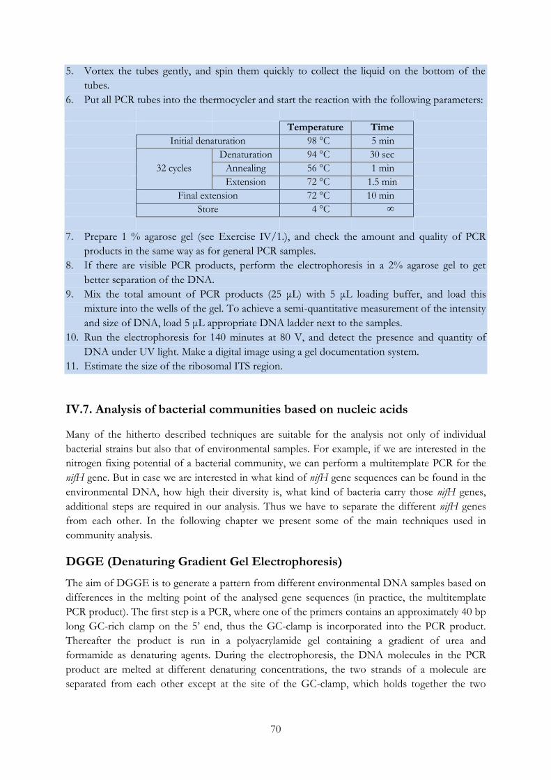
70
5. Vortex the tubes gently, and spin them quickly to collect the liquid on the bottom of the
tubes.
6. Put all PCR tubes into the thermocycler and start the reaction with the following parameters:
Temperature Time
Initial denaturation 98 °C 5 min
32 cycles
Denaturation 94 °C 30 sec
Annealing 56 °C 1 min
Extension 72 °C 1.5 mins
Final extension 72 °C 10 min
Store 4 °C ∞
7. Prepare 1 % agarose gel (see Exercise IV/1.), and check the amount and quality of PCR
products in the same way as for general PCR samples.
8. If there are visible PCR products, perform the electrophoresis in a 2% agarose gel to get
better separation of the DNA.
9. Mix the total amount of PCR products (25 μL) with 5 μL loading buffer, and load this
mixture into the wells of the gel. To achieve a semi-quantitative measurement of the intensity
and size of DNA, load 5 μL appropriate DNA ladder next to the samples.
10. Run the electrophoresis for 140 minutes at 80 V, and detect the presence and quantity of
DNA under UV light. Make a digital image using a gel documentation system.
11. Estimate the size of the ribosomal ITS region.
IV.7. Analysis of bacterial communities based on nucleic acids
Many of the hitherto described techniques are suitable for the analysis not only of individual
bacterial strains but also that of environmental samples. For example, if we are interested in the
nitrogen fixing potential of a bacterial community, we can perform a multitemplate PCR for the
nifH gene. But in case we are interested in what kind of nifH gene sequences can be found in the
environmental DNA, how high their diversity is, what kind of bacteria carry those nifH genes,
additional steps are required in our analysis. Thus we have to separate the different nifH genes
from each other. In the following chapter we present some of the main techniques used in
community analysis.
DGGE (Denaturing Gradient Gel Electrophoresis)
The aim of DGGE is to generate a pattern from different environmental DNA samples based on
differences in the melting point of the analysed gene sequences (in practice, the multitemplate
PCR product). The first step is a PCR, where one of the primers contains an approximately 40 bp
long GC-rich clamp on the 5’ end, thus the GC-clamp is incorporated into the PCR product.
Thereafter the product is run in a polyacrylamide gel containing a gradient of urea and
formamide as denaturing agents. During the electrophoresis, the DNA molecules in the PCR
product are melted at different denaturing concentrations, the two strands of a molecule are
separated from each other except at the site of the GC-clamp, which holds together the two
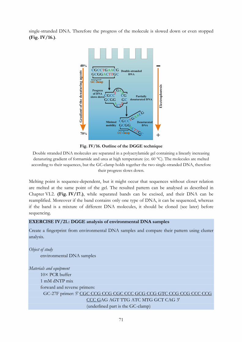
71
single-stranded DNA. Therefore the progress of the molecule is slowed down or even stopped
(Fig. IV/16.).
Fig. IV/16. Outline of the DGGE technique
Double stranded DNA molecules are separated in a polyacrylamide gel containing a linearly increasing
denaturing gradient of formamide and urea at high temperature (cc. 60 °C). The molecules are melted
according to their sequences, but the GC-clamp holds together the two single-stranded DNA, therefore
their progress slows down.
Melting point is sequence-dependent, but it might occur that sequences without closer relation
are melted at the same point of the gel. The resulted pattern can be analysed as described in
Chapter VI.2. (Fig. IV/17.), while separated bands can be excised, and their DNA can be
reamplified. Moreover if the band contains only one type of DNA, it can be sequenced, whereas
if the band is a mixture of different DNA molecules, it should be cloned (see later) before
sequencing.
EXERCISE IV/21.: DGGE analysis of environmental DNA samples
Create a fingerprint from environmental DNA samples and compare their pattern using cluster
analysis.
Object of study
environmental DNA samples
Materials and equipment
10× PCR buffer
1 mM dNTP mix
forward and reverse primers:
GC-27F primer: 5' CGC CCG CCG CGC CCC GCG CCG GTC CCG CCG CCC CCG
CCC GAG AGT TTG ATC MTG GCT CAG 3'
(underlined part is the GC-clamp)
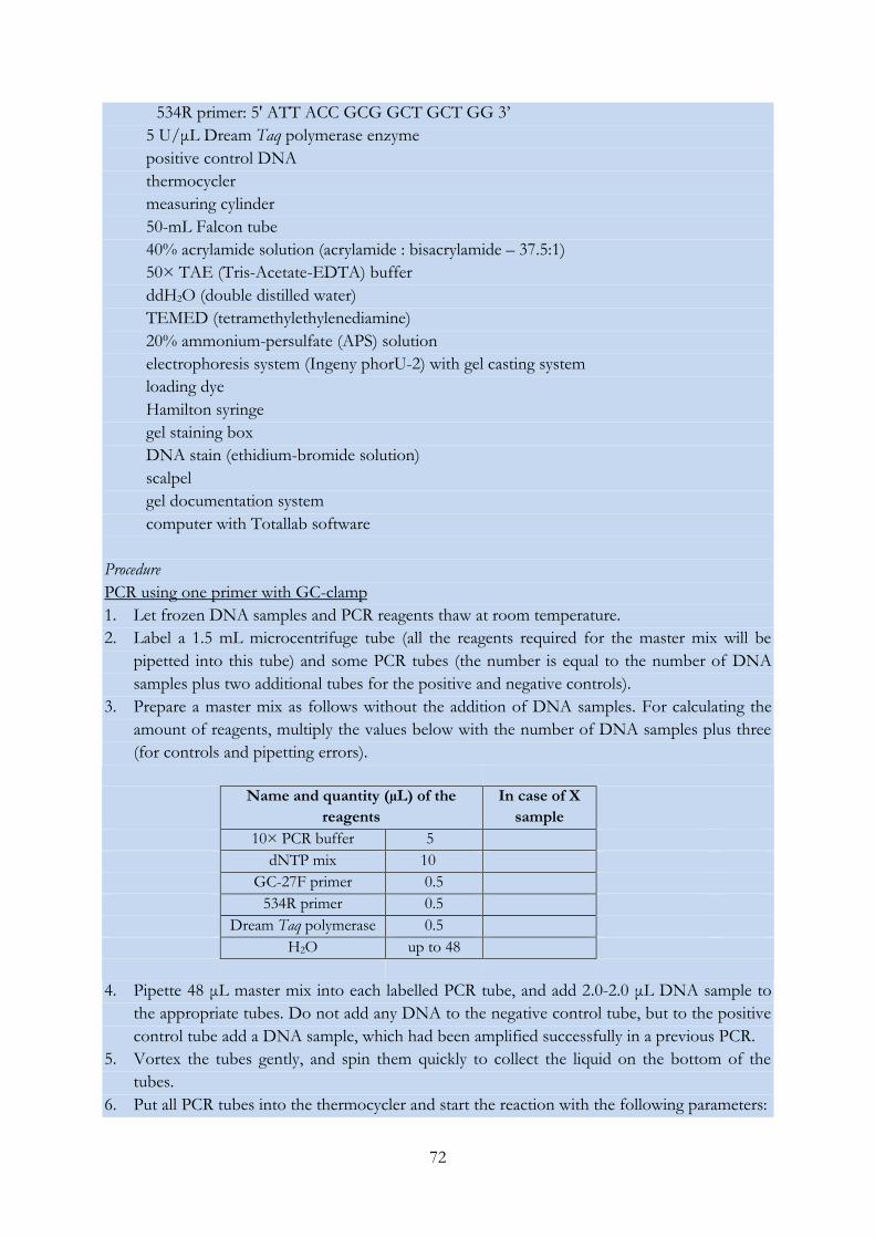
72
534R primer: 5' ATT ACC GCG GCT GCT GG 3’
5 U/μL Dream Taq polymerase enzyme
positive control DNA
thermocycler
measuring cylinder
50-mL Falcon tube
40% acrylamide solution (acrylamide : bisacrylamide – 37.5:1)
50× TAE (Tris-Acetate-EDTA) buffer
ddH2O (double distilled water)
TEMED (tetramethylethylenediamine)
20% ammonium-persulfate (APS) solution
electrophoresis system (Ingeny phorU-2) with gel casting system
loading dye
Hamilton syringe
gel staining box
DNA stain (ethidium-bromide solution)
scalpel
gel documentation system
computer with Totallab software
Procedure
PCR using one primer with GC-clamp
1. Let frozen DNA samples and PCR reagents thaw at room temperature.
2. Label a 1.5 mL microcentrifuge tube (all the reagents required for the master mix will be
pipetted into this tube) and some PCR tubes (the number is equal to the number of DNA
samples plus two additional tubes for the positive and negative controls).
3. Prepare a master mix as follows without the addition of DNA samples. For calculating the
amount of reagents, multiply the values below with the number of DNA samples plus three
(for controls and pipetting errors).
Name and quantity (µL) of the
reagents
In case of X
sample
10× PCR buffer 5
dNTP mix 10
GC-27F primer 0.5
534R primer 0.5
Dream Taq polymerase 0.5
H2O up to 48
4. Pipette 48 μL master mix into each labelled PCR tube, and add 2.0-2.0 μL DNA sample to
the appropriate tubes. Do not add any DNA to the negative control tube, but to the positive
control tube add a DNA sample, which had been amplified successfully in a previous PCR.
5. Vortex the tubes gently, and spin them quickly to collect the liquid on the bottom of the
tubes.
6. Put all PCR tubes into the thermocycler and start the reaction with the following parameters:
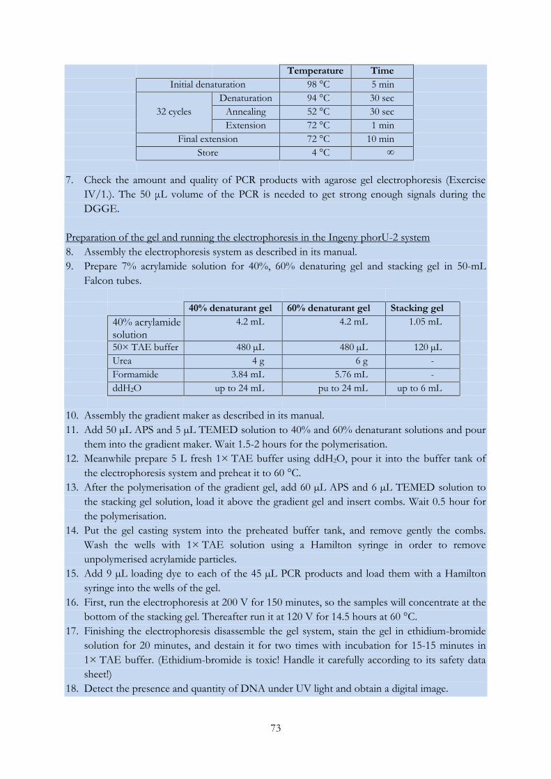
73
Temperature Time
Initial denaturation 98 °C 5 min
32 cycles
Denaturation 94 °C 30 sec
Annealing 52 °C 30 sec
Extension 72 °C 1 min
Final extension 72 °C 10 min
Store 4 °C ∞
7. Check the amount and quality of PCR products with agarose gel electrophoresis (Exercise
IV/1.). The 50 μL volume of the PCR is needed to get strong enough signals during the
DGGE.
Preparation of the gel and running the electrophoresis in the Ingeny phorU-2 system
8. Assembly the electrophoresis system as described in its manual.
9. Prepare 7% acrylamide solution for 40%, 60% denaturing gel and stacking gel in 50-mL
Falcon tubes.
40% denaturant gel 60% denaturant gel Stacking gel
40% acrylamide solution
4.2 mL 4.2 mL 1.05 mL
50× TAE buffer 480 µL 480 µL 120 µL
Urea 4 g 6 g -
Formamide 3.84 mL 5.76 mL -
ddH2O up to 24 mL pu to 24 mL up to 6 mL
10. Assembly the gradient maker as described in its manual.
11. Add 50 µL APS and 5 µL TEMED solution to 40% and 60% denaturant solutions and pour
them into the gradient maker. Wait 1.5-2 hours for the polymerisation.
12. Meanwhile prepare 5 L fresh 1× TAE buffer using ddH2O, pour it into the buffer tank of
the electrophoresis system and preheat it to 60 °C.
13. After the polymerisation of the gradient gel, add 60 µL APS and 6 µL TEMED solution to
the stacking gel solution, load it above the gradient gel and insert combs. Wait 0.5 hour for
the polymerisation.
14. Put the gel casting system into the preheated buffer tank, and remove gently the combs.
Wash the wells with 1× TAE solution using a Hamilton syringe in order to remove
unpolymerised acrylamide particles.
15. Add 9 µL loading dye to each of the 45 µL PCR products and load them with a Hamilton
syringe into the wells of the gel.
16. First, run the electrophoresis at 200 V for 150 minutes, so the samples will concentrate at the
bottom of the stacking gel. Thereafter run it at 120 V for 14.5 hours at 60 °C.
17. Finishing the electrophoresis disassemble the gel system, stain the gel in ethidium-bromide
solution for 20 minutes, and destain it for two times with incubation for 15-15 minutes in
1× TAE buffer. (Ethidium-bromide is toxic! Handle it carefully according to its safety data
sheet!)
18. Detect the presence and quantity of DNA under UV light and obtain a digital image.
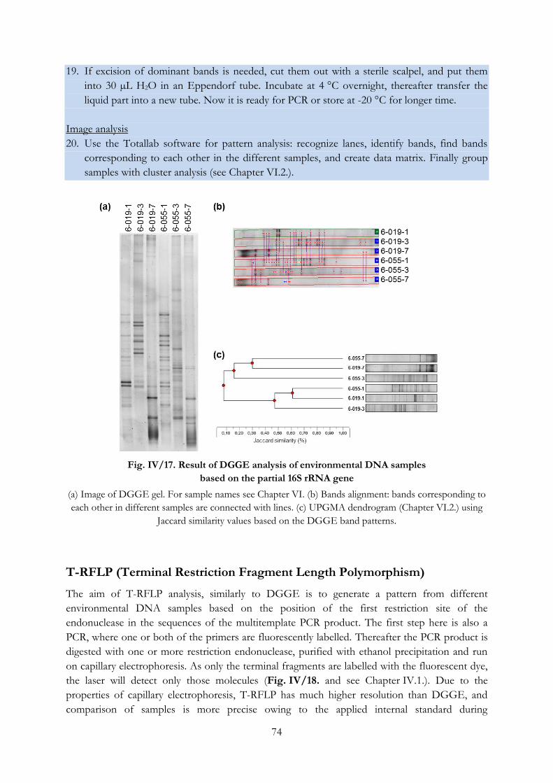
74
19. If excision of dominant bands is needed, cut them out with a sterile scalpel, and put them
into 30 µL H2O in an Eppendorf tube. Incubate at 4 °C overnight, thereafter transfer the
liquid part into a new tube. Now it is ready for PCR or store at -20 °C for longer time.
Image analysis
20. Use the Totallab software for pattern analysis: recognize lanes, identify bands, find bands
corresponding to each other in the different samples, and create data matrix. Finally group
samples with cluster analysis (see Chapter VI.2.).
Fig. IV/17. Result of DGGE analysis of environmental DNA samples
based on the partial 16S rRNA gene
(a) Image of DGGE gel. For sample names see Chapter VI. (b) Bands alignment: bands corresponding to
each other in different samples are connected with lines. (c) UPGMA dendrogram (Chapter VI.2.) using
Jaccard similarity values based on the DGGE band patterns.
T-RFLP (Terminal Restriction Fragment Length Polymorphism)
The aim of T-RFLP analysis, similarly to DGGE is to generate a pattern from different
environmental DNA samples based on the position of the first restriction site of the
endonuclease in the sequences of the multitemplate PCR product. The first step here is also a
PCR, where one or both of the primers are fluorescently labelled. Thereafter the PCR product is
digested with one or more restriction endonuclease, purified with ethanol precipitation and run
on capillary electrophoresis. As only the terminal fragments are labelled with the fluorescent dye,
the laser will detect only those molecules (Fig. IV/18. and see Chapter IV.1.). Due to the
properties of capillary electrophoresis, T-RFLP has much higher resolution than DGGE, and
comparison of samples is more precise owing to the applied internal standard during
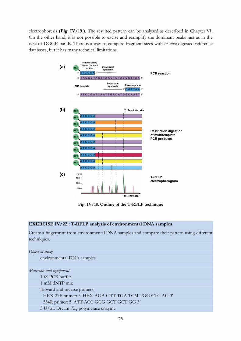
75
electrophoresis (Fig. IV/19.). The resulted pattern can be analysed as described in Chapter VI.
On the other hand, it is not possible to excise and reamplify the dominant peaks just as in the
case of DGGE bands. There is a way to compare fragment sizes with in silico digested reference
databases, but it has many technical limitations.
Fig. IV/18. Outline of the T-RFLP technique
EXERCISE IV/22.: T-RFLP analysis of environmental DNA samples
Create a fingerprint from environmental DNA samples and compare their pattern using different
techniques.
Object of study
environmental DNA samples
Materials and equipment
10× PCR buffer
1 mM dNTP mix
forward and reverse primers:
HEX-27F primer: 5' HEX-AGA GTT TGA TCM TGG CTC AG 3'
534R primer: 5' ATT ACC GCG GCT GCT GG 3’
5 U/μL Dream Taq polymerase enzyme
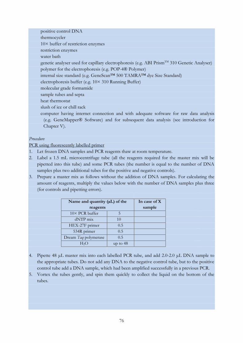
76
positive control DNA
thermocycler
10× buffer of restriction enzymes
restriction enzymes
water bath
genetic analyser used for capillary electrophoresis (e.g. ABI PrismTM 310 Genetic Analyser)
polymer for the electrophoresis (e.g. POP-4® Polymer)
internal size standard (e.g. GeneScan™ 500 TAMRA™ dye Size Standard)
electrophoresis buffer (e.g. 10× 310 Running Buffer)
molecular grade formamide
sample tubes and septa
heat thermostat
slush of ice or chill rack
computer having internet connection and with adequate software for raw data analysis
(e.g. GeneMapper® Software) and for subsequent data analysis (see introduction for
Chapter V).
Procedure
PCR using fluorescently labelled primer
1. Let frozen DNA samples and PCR reagents thaw at room temperature.
2. Label a 1.5 mL microcentrifuge tube (all the reagents required for the master mix will be
pipetted into this tube) and some PCR tubes (the number is equal to the number of DNA
samples plus two additional tubes for the positive and negative controls).
3. Prepare a master mix as follows without the addition of DNA samples. For calculating the
amount of reagents, multiply the values below with the number of DNA samples plus three
(for controls and pipetting errors).
Name and quantity (µL) of the
reagents
In case of X
sample
10× PCR buffer 5
dNTP mix 10
HEX-27F primer 0.5
534R primer 0.5
Dream Taq polymerase 0.5
H2O up to 48
4. Pipette 48 μL master mix into each labelled PCR tube, and add 2.0-2.0 μL DNA sample to
the appropriate tubes. Do not add any DNA to the negative control tube, but to the positive
control tube add a DNA sample, which had been amplified successfully in a previous PCR.
5. Vortex the tubes gently, and spin them quickly to collect the liquid on the bottom of the
tubes.
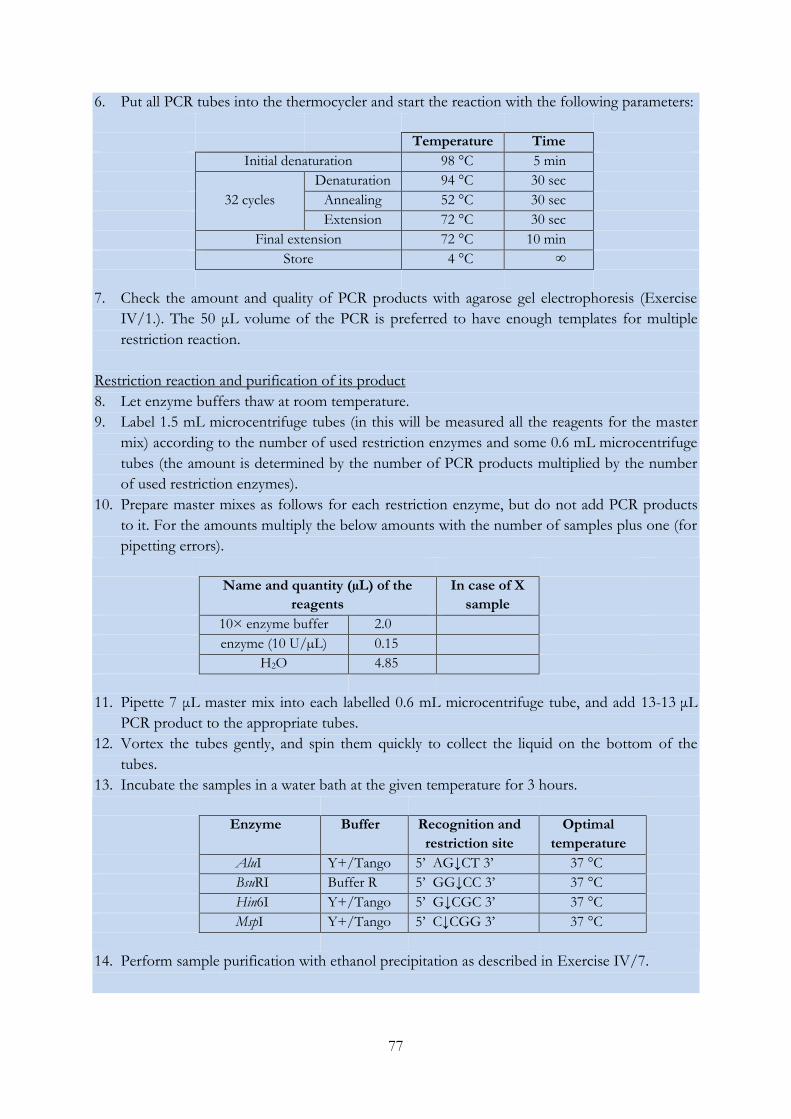
77
6. Put all PCR tubes into the thermocycler and start the reaction with the following parameters:
Temperature Time
Initial denaturation 98 °C 5 min
32 cycles
Denaturation 94 °C 30 sec
Annealing 52 °C 30 sec
Extension 72 °C 30 sec
Final extension 72 °C 10 min
Store 4 °C ∞
7. Check the amount and quality of PCR products with agarose gel electrophoresis (Exercise
IV/1.). The 50 μL volume of the PCR is preferred to have enough templates for multiple
restriction reaction.
Restriction reaction and purification of its product
8. Let enzyme buffers thaw at room temperature.
9. Label 1.5 mL microcentrifuge tubes (in this will be measured all the reagents for the master
mix) according to the number of used restriction enzymes and some 0.6 mL microcentrifuge
tubes (the amount is determined by the number of PCR products multiplied by the number
of used restriction enzymes).
10. Prepare master mixes as follows for each restriction enzyme, but do not add PCR products
to it. For the amounts multiply the below amounts with the number of samples plus one (for
pipetting errors).
Name and quantity (µL) of the
reagents
In case of X
sample
10× enzyme buffer 2.0
enzyme (10 U/µL) 0.15
H2O 4.85
11. Pipette 7 μL master mix into each labelled 0.6 mL microcentrifuge tube, and add 13-13 μL
PCR product to the appropriate tubes.
12. Vortex the tubes gently, and spin them quickly to collect the liquid on the bottom of the
tubes.
13. Incubate the samples in a water bath at the given temperature for 3 hours.
Enzyme Buffer Recognition and
restriction site
Optimal
temperature
AluI Y+/Tango 5’ AG↓CT 3’ 37 °C
BsuRI Buffer R 5’ GG↓CC 3’ 37 °C
Hin6I Y+/Tango 5’ G↓CGC 3’ 37 °C
MspI Y+/Tango 5’ C↓CGG 3’ 37 °C
14. Perform sample purification with ethanol precipitation as described in Exercise IV/7.
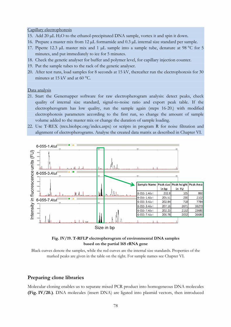
78
Capillary electrophoresis
15. Add 20 µL H2O to the ethanol-precipitated DNA sample, vortex it and spin it down.
16. Prepare a master mix from 12 µL formamide and 0.3 µL internal size standard per sample.
17. Pipette 12.3 µL master mix and 1 µL sample into a sample tube, denature at 98 °C for 5
minutes, and put immediately to ice for 5 minutes.
18. Check the genetic analyser for buffer and polymer level, for capillary injection counter.
19. Put the sample tubes to the rack of the genetic analyser.
20. After test runs, load samples for 8 seconds at 15 kV, thereafter run the electrophoresis for 30
minutes at 15 kV and at 60 °C.
Data analysis
21. Start the Genemapper software for raw electropherogram analysis: detect peaks, check
quality of internal size standard, signal-to-noise ratio and export peak table. If the
electropherogram has low quality, run the sample again (steps 16-20.) with modified
electrophoresis parameters according to the first run, so change the amount of sample
volume added to the master mix or change the duration of sample loading.
22. Use T-REX (trex.biohpc.org/index.aspx) or scripts in program R for noise filtration and
alignment of electropherograms. Analyse the created data matrix as described in Chapter VI.
Fig. IV/19. T-RFLP electropherogram of environmental DNA samples
based on the partial 16S rRNA gene
Black curves denote the samples, while the red curves are the internal size standards. Properties of the
marked peaks are given in the table on the right. For sample names see Chapter VI.
Preparing clone libraries
Molecular cloning enables us to separate mixed PCR product into homogeneous DNA molecules
(Fig. IV/20.). DNA molecules (insert DNA) are ligated into plasmid vectors, then introduced
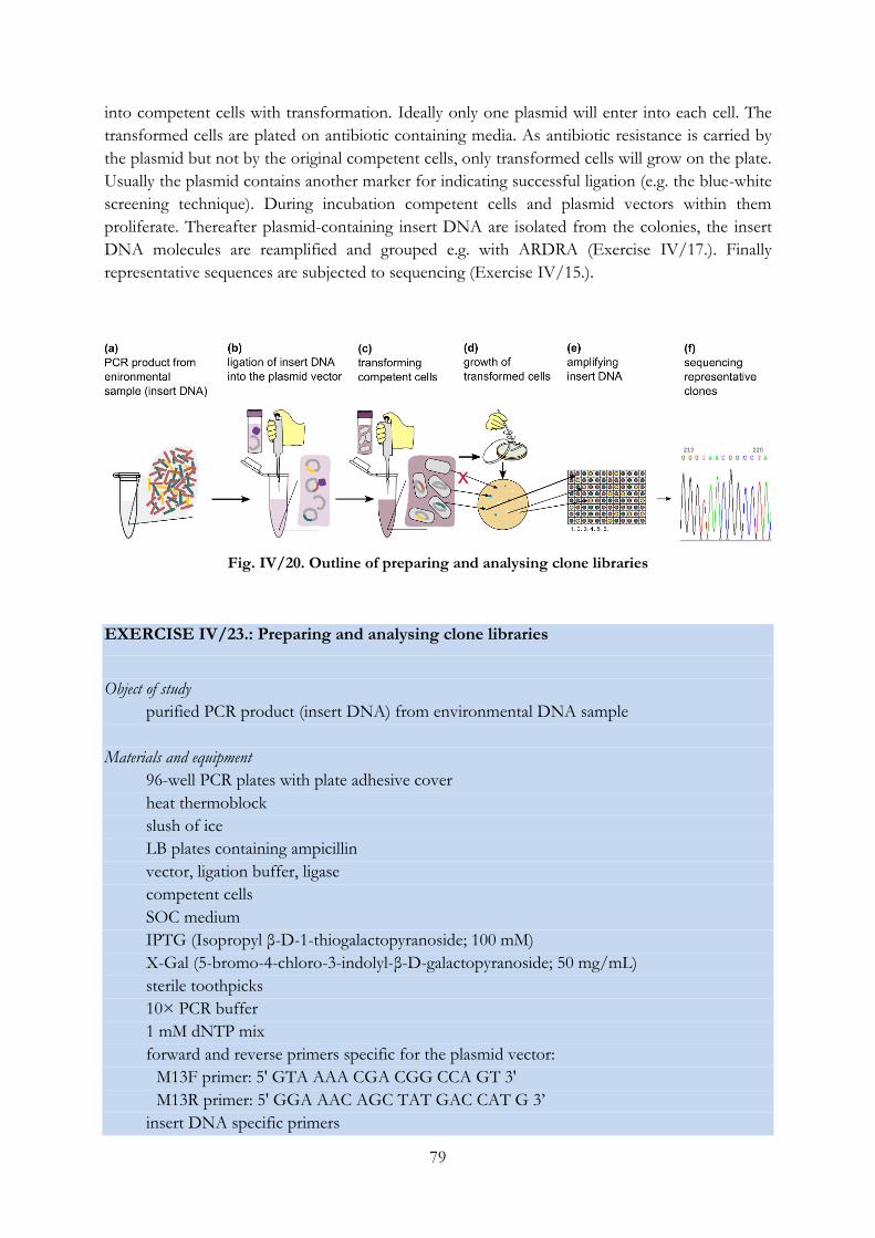
79
into competent cells with transformation. Ideally only one plasmid will enter into each cell. The
transformed cells are plated on antibiotic containing media. As antibiotic resistance is carried by
the plasmid but not by the original competent cells, only transformed cells will grow on the plate.
Usually the plasmid contains another marker for indicating successful ligation (e.g. the blue-white
screening technique). During incubation competent cells and plasmid vectors within them
proliferate. Thereafter plasmid-containing insert DNA are isolated from the colonies, the insert
DNA molecules are reamplified and grouped e.g. with ARDRA (Exercise IV/17.). Finally
representative sequences are subjected to sequencing (Exercise IV/15.).
Fig. IV/20. Outline of preparing and analysing clone libraries
EXERCISE IV/23.: Preparing and analysing clone libraries
Object of study
purified PCR product (insert DNA) from environmental DNA sample
Materials and equipment
96-well PCR plates with plate adhesive cover
heat thermoblock
slush of ice
LB plates containing ampicillin
vector, ligation buffer, ligase
competent cells
SOC medium
IPTG (Isopropyl β-D-1-thiogalactopyranoside; 100 mM)
X-Gal (5-bromo-4-chloro-3-indolyl-β-D-galactopyranoside; 50 mg/mL)
sterile toothpicks
10× PCR buffer
1 mM dNTP mix
forward and reverse primers specific for the plasmid vector:
M13F primer: 5' GTA AAA CGA CGG CCA GT 3'
M13R primer: 5' GGA AAC AGC TAT GAC CAT G 3’
insert DNA specific primers
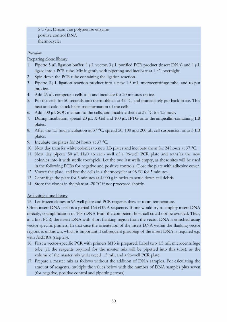
80
5 U/μL Dream Taq polymerase enzyme
positive control DNA
thermocycler
Procedure
Preparing clone library
1. Pipette 5 µL ligation buffer, 1 µL vector, 3 µL purified PCR product (insert DNA) and 1 µL
ligase into a PCR tube. Mix it gently with pipetting and incubate at 4 °C overnight.
2. Spin down the PCR tube containing the ligation reaction.
3. Pipette 2 µL ligation reaction product into a new 1.5 mL microcentrifuge tube, and to put
into ice.
4. Add 25 µL competent cells to it and incubate for 20 minutes on ice.
5. Put the cells for 50 seconds into thermoblock at 42 °C, and immediately put back to ice. This
heat and cold shock helps transformation of the cells.
6. Add 500 µL SOC medium to the cells, and incubate them at 37 °C for 1.5 hour.
7. During incubation, spread 20 µL X-Gal and 100 µL IPTG onto the ampicillin-containing LB
plates.
8. After the 1.5 hour incubation at 37 °C, spread 50, 100 and 200 µL cell suspension onto 3 LB
plates.
9. Incubate the plates for 24 hours at 37 °C.
10. Next day transfer white colonies to new LB plates and incubate them for 24 hours at 37 °C.
11. Next day pipette 50 µL H2O to each well of a 96-well PCR plate and transfer the new
colonies into it with sterile toothpick. Let the two last wells empty, as these sites will be used
in the following PCRs for negative and positive controls. Close the plate with adhesive cover.
12. Vortex the plate, and lyse the cells in a thermocycler at 98 °C for 5 minutes.
13. Centrifuge the plate for 3 minutes at 4,000 g in order to settle down cell debris.
14. Store the clones in the plate at -20 °C if not processed shortly.
Analysing clone library
15. Let frozen clones in 96-well plate and PCR reagents thaw at room temperature.
Often insert DNA itself is a partial 16S rDNA sequence. If one would try to amplify insert DNA
directly, coamplification of 16S rDNA from the competent host cell could not be avoided. Thus,
in a first PCR, the insert DNA with short flanking region from the vector DNA is enriched using
vector specific primers. In that case the orientation of the insert DNA within the flanking vector
regions is unknown, which is important if subsequent grouping of the insert DNA is required e.g.
with ARDRA (step 23).
16. First a vector-specific PCR with primers M13 is prepared. Label two 1.5 mL microcentrifuge
tube (all the reagents required for the master mix will be pipetted into this tube), as the
volume of the master mix will exceed 1.5 mL, and a 96-well PCR plate.
17. Prepare a master mix as follows without the addition of DNA samples. For calculating the
amount of reagents, multiply the values below with the number of DNA samples plus seven
(for negative, positive control and pipetting errors).
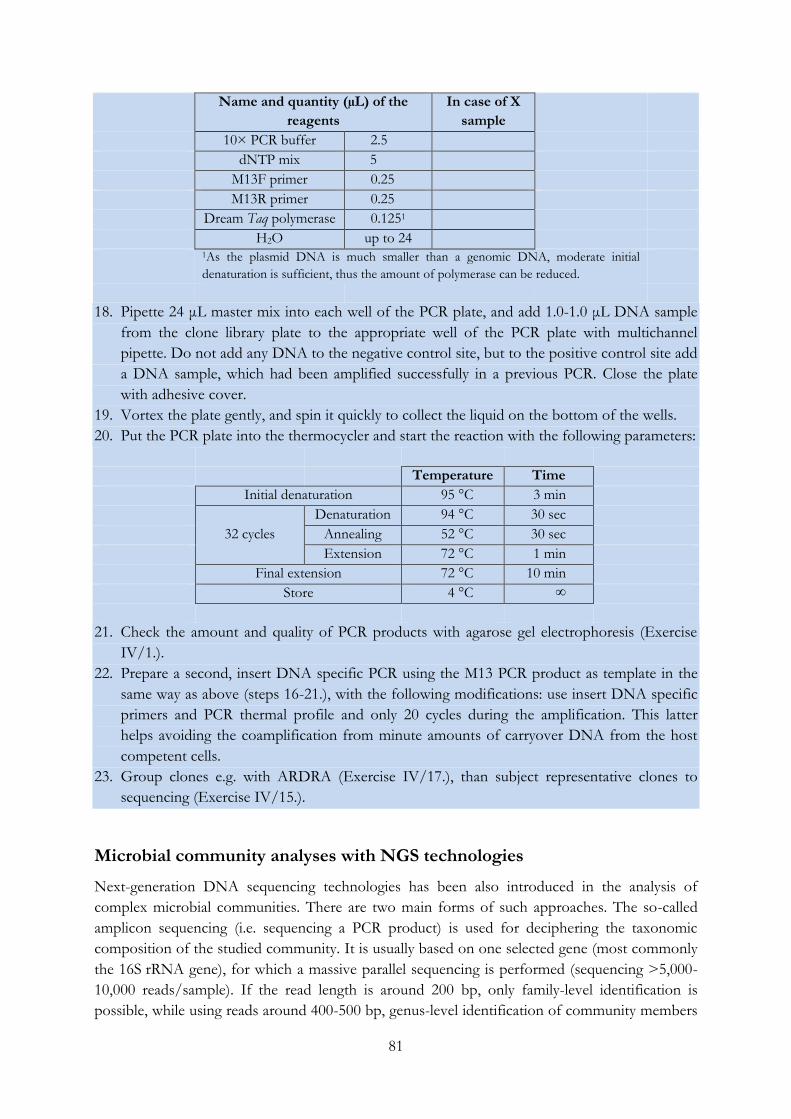
81
Name and quantity (µL) of the
reagents
In case of X
sample
10× PCR buffer 2.5
dNTP mix 5
M13F primer 0.25
M13R primer 0.25
Dream Taq polymerase 0.1251
H2O up to 24
1As the plasmid DNA is much smaller than a genomic DNA, moderate initial
denaturation is sufficient, thus the amount of polymerase can be reduced.
18. Pipette 24 μL master mix into each well of the PCR plate, and add 1.0-1.0 μL DNA sample
from the clone library plate to the appropriate well of the PCR plate with multichannel
pipette. Do not add any DNA to the negative control site, but to the positive control site add
a DNA sample, which had been amplified successfully in a previous PCR. Close the plate
with adhesive cover.
19. Vortex the plate gently, and spin it quickly to collect the liquid on the bottom of the wells.
20. Put the PCR plate into the thermocycler and start the reaction with the following parameters:
Temperature Time
Initial denaturation 95 °C 3 min
32 cycles
Denaturation 94 °C 30 sec
Annealing 52 °C 30 sec
Extension 72 °C 1 min
Final extension 72 °C 10 min
Store 4 °C ∞
21. Check the amount and quality of PCR products with agarose gel electrophoresis (Exercise
IV/1.).
22. Prepare a second, insert DNA specific PCR using the M13 PCR product as template in the
same way as above (steps 16-21.), with the following modifications: use insert DNA specific
primers and PCR thermal profile and only 20 cycles during the amplification. This latter
helps avoiding the coamplification from minute amounts of carryover DNA from the host
competent cells.
23. Group clones e.g. with ARDRA (Exercise IV/17.), than subject representative clones to
sequencing (Exercise IV/15.).
Microbial community analyses with NGS technologies
Next-generation DNA sequencing technologies has been also introduced in the analysis of
complex microbial communities. There are two main forms of such approaches. The so-called
amplicon sequencing (i.e. sequencing a PCR product) is used for deciphering the taxonomic
composition of the studied community. It is usually based on one selected gene (most commonly
the 16S rRNA gene), for which a massive parallel sequencing is performed (sequencing >5,000-
10,000 reads/sample). If the read length is around 200 bp, only family-level identification is
possible, while using reads around 400-500 bp, genus-level identification of community members
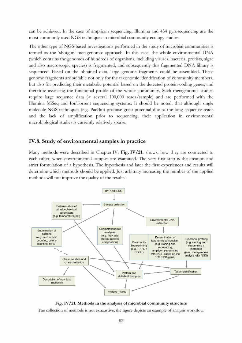
82
can be achieved. In the case of amplicon sequencing, Illumina and 454 pyrosequencing are the
most commonly used NGS techniques in microbial community ecology studies.
The other type of NGS-based investigations performed in the study of microbial communities is
termed as the ’shotgun’ metagenomic approach. In this case, the whole environmental DNA
(which contains the genomes of hundreds of organisms, including viruses, bacteria, protists, algae
and also macroscopic species) is fragmented, and subsequently this fragmented DNA library is
sequenced. Based on the obtained data, large genome fragments could be assembled. These
genome fragments are suitable not only for the taxonomic identification of community members,
but also for predicting their metabolic potential based on the detected protein-coding genes, and
therefore assessing the functional profile of the whole community. Such metagenomic studies
require large sequence data (> several 100,000 reads/sample) and are performed with the
Illumina MiSeq and IonTorrent sequencing systems. It should be noted, that although single
molecule NGS techniques (e.g. PacBio) promise great potential due to the long sequence reads
and the lack of amplification prior to sequencing, their application in environmental
microbiological studies is currently relatively sparse.
IV.8. Study of environmental samples in practice
Many methods were described in Chapter IV. Fig. IV/21. shows, how they are connected to
each other, when environmental samples are examined. The very first step is the creation and
strict formulation of a hypothesis. The hypothesis and later the first experiences and results will
determine which methods should be applied. Just arbitrary increasing the number of the applied
methods will not improve the quality of the results!
Fig. IV/21. Methods in the analysis of microbial community structure
The collection of methods is not exhaustive, the figure depicts an example of analysis workflow.
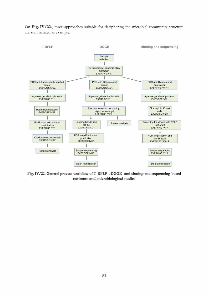
83
On Fig. IV/22., three approaches suitable for deciphering the microbial community structure
are summarized as example.
Fig. IV/22. General process workflow of T-RFLP-, DGGE- and cloning and sequencing-based
environmental microbiological studies
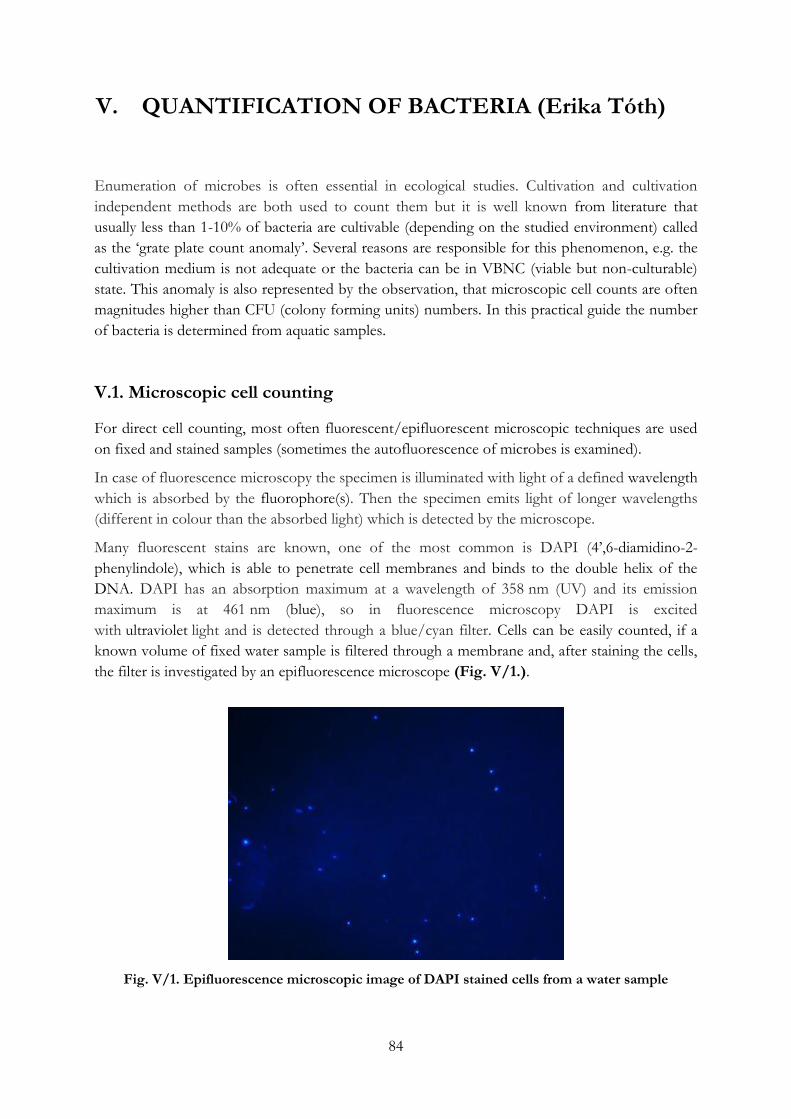
84
V. QUANTIFICATION OF BACTERIA (Erika Tóth)
Enumeration of microbes is often essential in ecological studies. Cultivation and cultivation
independent methods are both used to count them but it is well known from literature that
usually less than 1-10% of bacteria are cultivable (depending on the studied environment) called
as the ‘grate plate count anomaly’. Several reasons are responsible for this phenomenon, e.g. the
cultivation medium is not adequate or the bacteria can be in VBNC (viable but non-culturable)
state. This anomaly is also represented by the observation, that microscopic cell counts are often
magnitudes higher than CFU (colony forming units) numbers. In this practical guide the number
of bacteria is determined from aquatic samples.
V.1. Microscopic cell counting
For direct cell counting, most often fluorescent/epifluorescent microscopic techniques are used
on fixed and stained samples (sometimes the autofluorescence of microbes is examined).
In case of fluorescence microscopy the specimen is illuminated with light of a defined wavelength
which is absorbed by the fluorophore(s). Then the specimen emits light of longer wavelengths
(different in colour than the absorbed light) which is detected by the microscope.
Many fluorescent stains are known, one of the most common is DAPI (4’,6-diamidino-2-
phenylindole), which is able to penetrate cell membranes and binds to the double helix of the
DNA. DAPI has an absorption maximum at a wavelength of 358 nm (UV) and its emission
maximum is at 461 nm (blue), so in fluorescence microscopy DAPI is excited
with ultraviolet light and is detected through a blue/cyan filter. Cells can be easily counted, if a
known volume of fixed water sample is filtered through a membrane and, after staining the cells,
the filter is investigated by an epifluorescence microscope (Fig. V/1.).
Fig. V/1. Epifluorescence microscopic image of DAPI stained cells from a water sample
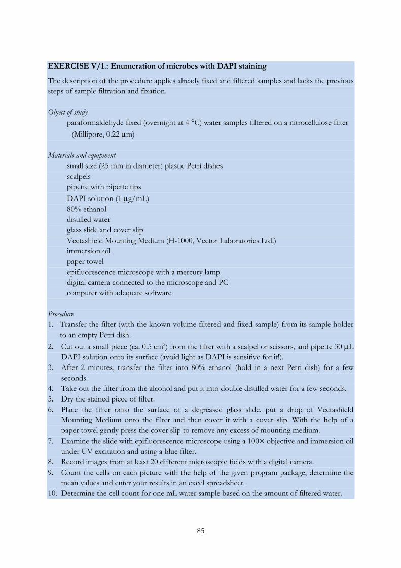
85
EXERCISE V/1.: Enumeration of microbes with DAPI staining
The description of the procedure applies already fixed and filtered samples and lacks the previous
steps of sample filtration and fixation.
Object of study
paraformaldehyde fixed (overnight at 4 °C) water samples filtered on a nitrocellulose filter
(Millipore, 0.22 m)
Materials and equipment
small size (25 mm in diameter) plastic Petri dishes
scalpels
pipette with pipette tips
DAPI solution (1 g/mL)
80% ethanol
distilled water
glass slide and cover slip
Vectashield Mounting Medium (H-1000, Vector Laboratories Ltd.)
immersion oil
paper towel
epifluorescence microscope with a mercury lamp
digital camera connected to the microscope and PC
computer with adequate software
Procedure
1. Transfer the filter (with the known volume filtered and fixed sample) from its sample holder
to an empty Petri dish.
2. Cut out a small piece (ca. 0.5 cm2) from the filter with a scalpel or scissors, and pipette 30 L
DAPI solution onto its surface (avoid light as DAPI is sensitive for it!).
3. After 2 minutes, transfer the filter into 80% ethanol (hold in a next Petri dish) for a few
seconds.
4. Take out the filter from the alcohol and put it into double distilled water for a few seconds.
5. Dry the stained piece of filter.
6. Place the filter onto the surface of a degreased glass slide, put a drop of Vectashield
Mounting Medium onto the filter and then cover it with a cover slip. With the help of a
paper towel gently press the cover slip to remove any excess of mounting medium.
7. Examine the slide with epifluorescence microscope using a 100× objective and immersion oil
under UV excitation and using a blue filter.
8. Record images from at least 20 different microscopic fields with a digital camera.
9. Count the cells on each picture with the help of the given program package, determine the
mean values and enter your results in an excel spreadsheet.
10. Determine the cell count for one mL water sample based on the amount of filtered water.

86
V.2. Quantification of different bacteria based on MPN method
MPN (Most Probable Number) is often used to quantify different types of bacteria from natural
waters. The test is able to estimate the number of viable (and growing) microorganisms in a
sample after borderline dilutions, After the incubation period, estimation of microbial germ count
is possible using statistical tables based on the number of positive tubes/wells (showing
characteristic microbial growth: change in optical density, shifting of pH, changing of redox
values and subsequently colour, etc.). This method presumes that in the liquid medium the
distribution of cells is uniform, cells do not clump together and that there is detectable growth
even if only one viable microbial cell is present in the tube/well. The applied medium determines
which type of bacteria can be enumerated (total germ count, coliform bacteria, etc.).
EXERCISE V/2.: Determination the total germ count of surface waters with the MPN
method
Object of study
water sample from a natural aquatic habitat (e.g. Danube)
Materials and equipment
pipette, sterile tips
sterile Eppendorf tubes
sterile microtiter plate
medium for cultivation (adequate to cultivate heterotrophic bacteria, e.g. nutrient,
R2A medium)
microplate reader (Tecan Sunrise)
MPN table to evaluate data
Procedure
1. Measure 1350 L medium to 8 different Eppendorf tubes.
2. Make a dilution series in the medium (1350 L medium and 150 L sample).
3. From all dilutions pipette 250 L to the wells of the microtiter plate in 5 parallels in each
case.
4. Incubate it at room temperature for several days.
5. Check the optical density (OD) of the wells at 620 nm with a microplate reader after 24 and
48 hrs (if possible even later).
6. Calculate the cell number values with Garthright and Blodgett’s MPN-calculator
(www.fda.gov/downloads/Food/FoodScienceResearch/UCM164329.zip).
Quantification of hygienically relevant bacteria – study of faecal indicator
organisms
In hygienic practise, indicator organisms are used to qualify the pollution of different waters
(natural waters, drinking waters, etc.). Their presence in the water indicates whether the water is
contaminated by faeces or not. Indicator organisms must be present everywhere where pathogens
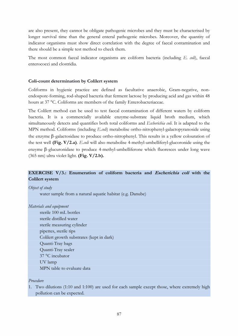
87
are also present, they cannot be obligate pathogenic microbes and they must be characterised by
longer survival time than the general enteral pathogenic microbes. Moreover, the quantity of
indicator organisms must show direct correlation with the degree of faecal contamination and
there should be a simple test method to check them.
The most common faecal indicator organisms are coliform bacteria (including E. coli), faecal
enterococci and clostridia.
Coli-count determination by Colilert system
Coliforms in hygienic practice are defined as facultative anaerobic, Gram-negative, non-
endospore-forming, rod-shaped bacteria that ferment lactose by producing acid and gas within 48
hours at 37 °C. Coliforms are members of the family Enterobacteriaceae.
The Colilert method can be used to test faecal contamination of different waters by coliform
bacteria. It is a commercially available enzyme-substrate liquid broth medium, which
simultaneously detects and quantifies both total coliforms and Escherichia coli. It is adapted to the
MPN method. Coliforms (including E.coli) metabolise ortho-nitrophenyl-galactopyranoside using
the enzyme -galactosidase to produce ortho-nitrophenyl. This results in a yellow colouration of
the test well (Fig. V/2.a). E.coli will also metabolise 4-methyl-umbelliferyl-glucoronide using the
enzyme -glucuronidase to produce 4-methyl-umbelliferone which fluoresces under long wave
(365 nm) ultra violet light. (Fig. V/2.b).
EXERCISE V/3.: Enumeration of coliform bacteria and Escherichia coli with the
Colilert system
Object of study
water sample from a natural aquatic habitat (e.g. Danube)
Materials and equipment
sterile 100 mL bottles
sterile distilled water
sterile measuring cylinder
pipettes, sterile tips
Colilert growth substrates (kept in dark)
Quanti-Tray bags
Quanti-Tray sealer
37 °C incubator
UV lamp
MPN table to evaluate data
Procedure
1. Two dilutions (1:10 and 1:100) are used for each sample except those, where extremely high
pollution can be expected.
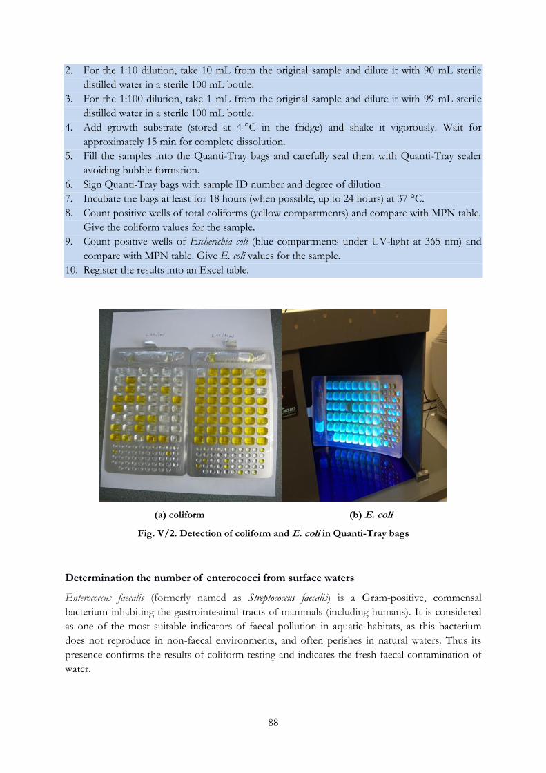
88
2. For the 1:10 dilution, take 10 mL from the original sample and dilute it with 90 mL sterile
distilled water in a sterile 100 mL bottle.
3. For the 1:100 dilution, take 1 mL from the original sample and dilute it with 99 mL sterile
distilled water in a sterile 100 mL bottle.
4. Add growth substrate (stored at 4 °C in the fridge) and shake it vigorously. Wait for
approximately 15 min for complete dissolution.
5. Fill the samples into the Quanti-Tray bags and carefully seal them with Quanti-Tray sealer
avoiding bubble formation.
6. Sign Quanti-Tray bags with sample ID number and degree of dilution.
7. Incubate the bags at least for 18 hours (when possible, up to 24 hours) at 37 °C.
8. Count positive wells of total coliforms (yellow compartments) and compare with MPN table.
Give the coliform values for the sample.
9. Count positive wells of Escherichia coli (blue compartments under UV-light at 365 nm) and
compare with MPN table. Give E. coli values for the sample.
10. Register the results into an Excel table.
(a) coliform (b) E. coli
Fig. V/2. Detection of coliform and E. coli in Quanti-Tray bags
Determination the number of enterococci from surface waters
Enterococcus faecalis (formerly named as Streptococcus faecalis) is a Gram-positive, commensal
bacterium inhabiting the gastrointestinal tracts of mammals (including humans). It is considered
as one of the most suitable indicators of faecal pollution in aquatic habitats, as this bacterium
does not reproduce in non-faecal environments, and often perishes in natural waters. Thus its
presence confirms the results of coliform testing and indicates the fresh faecal contamination of
water.
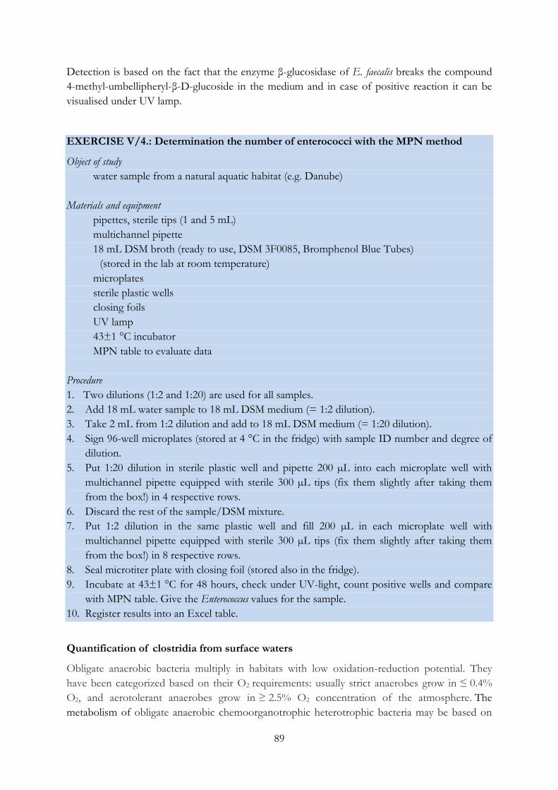
89
Detection is based on the fact that the enzyme β-glucosidase of E. faecalis breaks the compound
4-methyl-umbellipheryl-β-D-glucoside in the medium and in case of positive reaction it can be
visualised under UV lamp.
EXERCISE V/4.: Determination the number of enterococci with the MPN method
Object of study
water sample from a natural aquatic habitat (e.g. Danube)
Materials and equipment
pipettes, sterile tips (1 and 5 mL)
multichannel pipette
18 mL DSM broth (ready to use, DSM 3F0085, Bromphenol Blue Tubes)
(stored in the lab at room temperature)
microplates
sterile plastic wells
closing foils
UV lamp
43±1 °C incubator
MPN table to evaluate data
Procedure
1. Two dilutions (1:2 and 1:20) are used for all samples.
2. Add 18 mL water sample to 18 mL DSM medium (= 1:2 dilution).
3. Take 2 mL from 1:2 dilution and add to 18 mL DSM medium (= 1:20 dilution).
4. Sign 96-well microplates (stored at 4 °C in the fridge) with sample ID number and degree of
dilution.
5. Put 1:20 dilution in sterile plastic well and pipette 200 µL into each microplate well with
multichannel pipette equipped with sterile 300 µL tips (fix them slightly after taking them
from the box!) in 4 respective rows.
6. Discard the rest of the sample/DSM mixture.
7. Put 1:2 dilution in the same plastic well and fill 200 µL in each microplate well with
multichannel pipette equipped with sterile 300 µL tips (fix them slightly after taking them
from the box!) in 8 respective rows.
8. Seal microtiter plate with closing foil (stored also in the fridge).
9. Incubate at 43±1 °C for 48 hours, check under UV-light, count positive wells and compare
with MPN table. Give the Enterococcus values for the sample.
10. Register results into an Excel table.
Quantification of clostridia from surface waters
Obligate anaerobic bacteria multiply in habitats with low oxidation-reduction potential. They
have been categorized based on their O2 requirements: usually strict anaerobes grow in ≤ 0.4%
O2, and aerotolerant anaerobes grow in ≥ 2.5% O2 concentration of the atmosphere. The
metabolism of obligate anaerobic chemoorganotrophic heterotrophic bacteria may be based on
90
fermentation or anaerobic respiration. The appropriate method for the cultivation of these
bacteria should be chosen with considering the sensitivity of the given organism to oxygen
concentration and/or redox value within the media.
C. perfringens is a Gram-positive, rod-shaped, anaerobic, pathogenic bacterium. Due to its
endospores it survives in surface waters for a relatively long period, therefore its presence can
indicate old faecal pollution of surface waters.
EXERCISE V/5.: Determination of Clostridium perfringens from surface waters
Object of study
water sample from a natural aquatic habitat (e.g. Danube)
Materials and equipment
250 mL sterile bottle
60 °C water bath
0.45 μm pore-size cellulose nitrate membrane filter
sterile filtration equipment
distilled water
pipettes, sterile tips
tweezers
TSC (Tryptose Sulphite Cycloserine) agar medium (ready to use)
anaerobic indicator strip
anaerobic bags with stick
Procedure
1. Pasteurise 120 mL water sample in a sterile 250 mL glass bottle in a water bath (60 °C, for 15
min).
2. Filter 100 mL, 10 mL and 1 mL (amended with at least 10 mL of sterile distilled water)
through sterile 0.45 µm pore-size cellulose nitrate membrane filters in separate sterile
filtration units.
3. Put filters with sterile tweezers onto pre-dried TSC agar plates. Put the agar plates into
anaerobic bags, add an anaerobic indicator strip dipped in water and oxygen-binding sachet
(open carefully - there are different types of sachets, the one which is needed to fill with
water, you have to add 8 mL distilled water).
4. After it immediately close the bag with stick. Incubate at 44 °C for 21 hours.
5. Count light brown, brown, black colonies immediately after opening the anaerobic bag.
6. Take photographs of appropriate dilutions (Fig. V/3.). Give the number of clostridia in the
sample.
7. Register results into an Excel table.
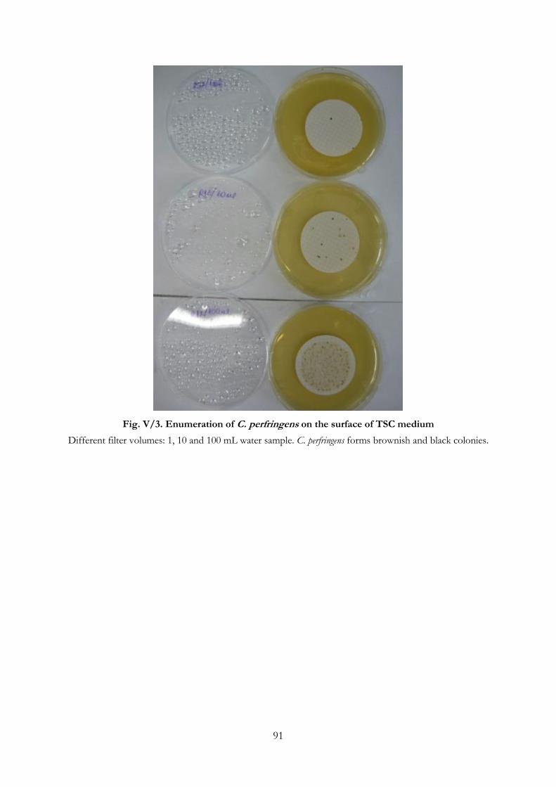
91
Fig. V/3. Enumeration of C. perfringens on the surface of TSC medium
Different filter volumes: 1, 10 and 100 mL water sample. C. perfringens forms brownish and black colonies.
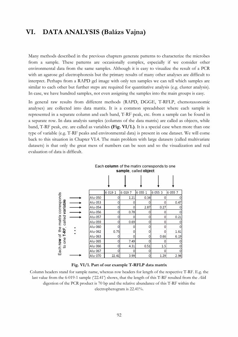
92
VI. DATA ANALYSIS (Balázs Vajna)
Many methods described in the previous chapters generate patterns to characterize the microbes
from a sample. These patterns are occasionally complex, especially if we consider other
environmental data from the same samples. Although it is easy to visualize the result of a PCR
with an agarose gel electrophoresis but the primary results of many other analyses are difficult to
interpret. Perhaps from a RAPD gel image with only ten samples we can tell which samples are
similar to each other but further steps are required for quantitative analysis (e.g. cluster analysis).
In case, we have hundred samples, not even assigning the samples into the main groups is easy.
In general raw results from different methods (RAPD, DGGE, T-RFLP, chemotaxonomic
analyses) are collected into data matrix. It is a common spreadsheet where each sample is
represented in a separate column and each band, T-RF peak, etc. from a sample can be found in
a separate row. In data analysis samples (columns of the data matrix) are called as objects, while
band, T-RF peak, etc. are called as variables (Fig. VI/1.). It is a special case when more than one
type of variable (e.g. T-RF peaks and environmental data) is present in one dataset. We will come
back to this situation in Chapter VI.4. The main problem with large datasets (called multivariate
datasets) is that only the great mess of numbers can be seen and so the visualization and real
evaluation of data is difficult.
Fig. VI/1. Part of our example T-RFLP data matrix
Column headers stand for sample name, whereas row headers for length of the respective T-RF. E.g. the
last value from the 6-019-1 sample (‘22.41’) shows, that the length of this T-RF resulted from the AluI
digestion of the PCR product is 70 bp and the relative abundance of this T-RF within the
electropherogram is 22.41%.
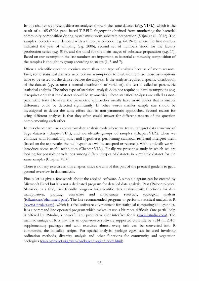
93
In this chapter we present different analyses through the same dataset (Fig. VI/1.), which is the
result of a 16S rRNA gene based T-RFLP fingerprint obtained from monitoring the bacterial
community composition during oyster mushroom substrate preparation (Vajna et al., 2012). The
samples (objects) were denoted with a three-parted-code (e.g. 6-019-1), where the first number
indicated the year of sampling (e.g. 2006), second set of numbers stood for the factory
production series (e.g. 019), and the third for the main stages of substrate preparation (e.g. 1st).
Based on our assumption the last numbers are important, as bacterial community composition of
the samples is thought to group according to stages (1, 3 and 7).
Often a scientific question requires more than one type of analysis because of more reasons.
First, some statistical analyses need certain assumptions to evaluate them, so those assumptions
have to be tested on the dataset before the analysis. If the analysis requires a specific distribution
of the dataset (e.g. assume a normal distribution of variables), the test is called as parametric
statistical analysis. The other type of statistical analysis does not require so hard assumptions (e.g.
it requires only that the dataset should be symmetric). These statistical analyses are called as non-
parametric tests. However the parametric approaches usually have more power that is smaller
difference could be detected significantly. In other words smaller sample size should be
investigated to detect the same effect than in non-parametric approaches. Second reason for
using different analyses is that they often could answer for different aspects of the question
complementing each other.
In this chapter we use exploratory data analysis tools where we try to interpret data structure of
large datasets (Chapter VI.1.), and we identify groups of samples (Chapter VI.2.). Then we
continue with formulating strict null hypotheses performing statistical tests and interpret them
(based on the test results the null hypothesis will be accepted or rejected). Without details we will
introduce some useful techniques (Chapter VI.3.). Finally we present a study in which we are
looking for possible correlations among different types of datasets in a multiple dataset for the
same samples (Chapter VI.4.).
There is not any exercise in this chapter, since the aim of this part of the practical guide is to get a
general overview in data analysis.
Finally let us give a few words about the applied software. A simple diagram can be created by
Microsoft Excel but it is not a dedicated program for detailed data analysis. Past (Paleontological
Statistics) is a free, user friendly program for scientific data analysis with functions for data
manipulation, plotting, univariate and multivariate statistics, ecological analysis
(folk.uio.no/ohammer/past). The last recommended program to perform statistical analysis is R
(www.r-project.org), which is a free software environment for statistical computing and graphics.
It is a command line operated program which makes its use a bit more difficult. One partial help
is offered by RStudio, a powerful and productive user interface for R (www.rstudio.com). The
main advantage of R is that it is an open-source software supported currently by 7814 (in 2016)
supplementary packages and with exercises almost every task can be converted into R
commands, the so-called scripts. For special analysis, package vegan can be used involving
ordination methods, diversity analysis and other functions for community and vegetation
ecologists (cran.r-project.org/web/packages/vegan/index.html).
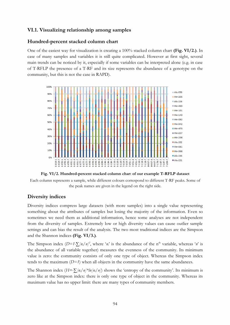
94
VI.1. Visualizing relationship among samples
Hundred-percent stacked column chart
One of the easiest way for visualization is creating a 100% stacked column chart (Fig. VI/2.). In
case of many samples and variables it is still quite complicated. However at first sight, several
main trends can be noticed by it, especially if some variables can be interpreted alone (e.g. in case
of T-RFLP the presence of a T-RF and its size represents the abundance of a genotype on the
community, but this is not the case in RAPD).
Fig. VI/2. Hundred-percent stacked column chart of our example T-RFLP dataset
Each column represents a sample, while different colours correspond to different T-RF peaks. Some of
the peak names are given in the legend on the right side.
Diversity indices
Diversity indices compress large datasets (with more samples) into a single value representing
something about the attributes of samples but losing the majority of the information. Even so
sometimes we need them as additional information, hence some analyses are not independent
from the diversity of samples. Extremely low or high diversity values can cause outlier sample
settings and can bias the result of the analysis. The two most traditional indices are the Simpson
and the Shannon indices (Fig. VI/3.).
The Simpson index (D=1-∑[ni/n]2, where ‘ni’ is the abundance of the nth variable, whereas ‘n’ is
the abundance of all variable together) measures the evenness of the community. Its minimum
value is zero: the community consists of only one type of object. Whereas the Simpson index
tends to the maximum (D=1) when all objects in the community have the same abundances.
The Shannon index (H=-∑[ni/n]*ln[ni/n]) shows the ‘entropy of the community’. Its minimum is
zero like at the Simpson index: there is only one type of object in the community. Whereas its
maximum value has no upper limit: there are many types of community members.
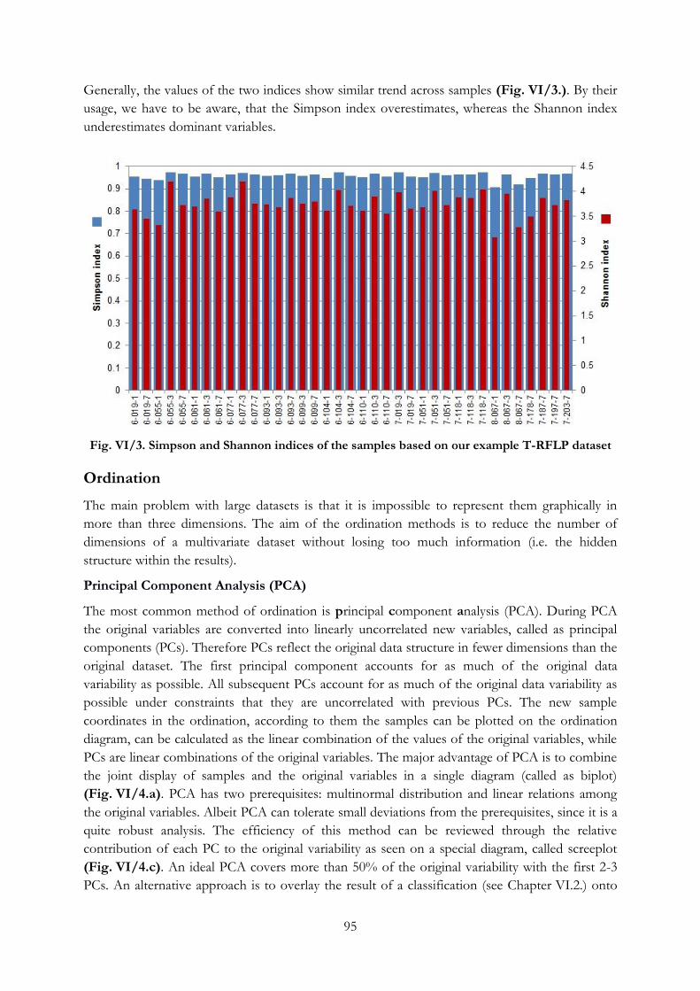
95
Generally, the values of the two indices show similar trend across samples (Fig. VI/3.). By their
usage, we have to be aware, that the Simpson index overestimates, whereas the Shannon index
underestimates dominant variables.
Fig. VI/3. Simpson and Shannon indices of the samples based on our example T-RFLP dataset
Ordination
The main problem with large datasets is that it is impossible to represent them graphically in
more than three dimensions. The aim of the ordination methods is to reduce the number of
dimensions of a multivariate dataset without losing too much information (i.e. the hidden
structure within the results).
Principal Component Analysis (PCA)
The most common method of ordination is principal component analysis (PCA). During PCA
the original variables are converted into linearly uncorrelated new variables, called as principal
components (PCs). Therefore PCs reflect the original data structure in fewer dimensions than the
original dataset. The first principal component accounts for as much of the original data
variability as possible. All subsequent PCs account for as much of the original data variability as
possible under constraints that they are uncorrelated with previous PCs. The new sample
coordinates in the ordination, according to them the samples can be plotted on the ordination
diagram, can be calculated as the linear combination of the values of the original variables, while
PCs are linear combinations of the original variables. The major advantage of PCA is to combine
the joint display of samples and the original variables in a single diagram (called as biplot)
(Fig. VI/4.a). PCA has two prerequisites: multinormal distribution and linear relations among
the original variables. Albeit PCA can tolerate small deviations from the prerequisites, since it is a
quite robust analysis. The efficiency of this method can be reviewed through the relative
contribution of each PC to the original variability as seen on a special diagram, called screeplot
(Fig. VI/4.c). An ideal PCA covers more than 50% of the original variability with the first 2-3
PCs. An alternative approach is to overlay the result of a classification (see Chapter VI.2.) onto
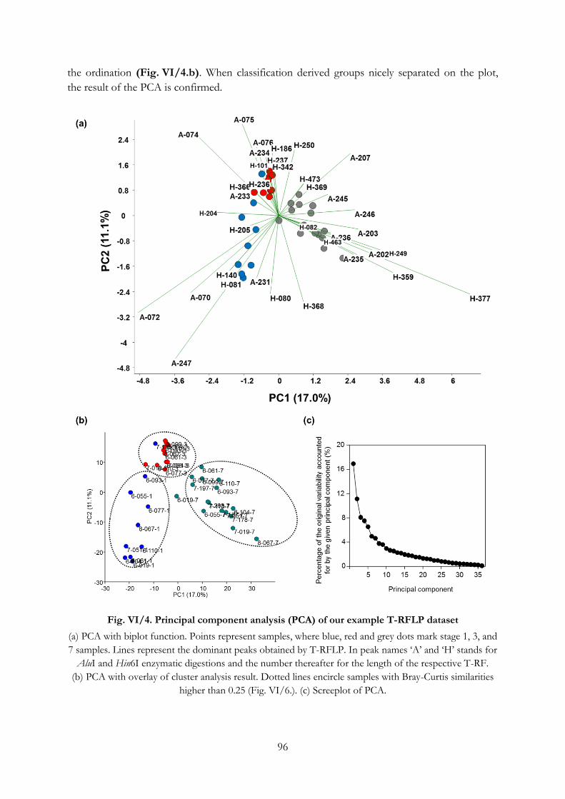
96
the ordination (Fig. VI/4.b). When classification derived groups nicely separated on the plot,
the result of the PCA is confirmed.
Fig. VI/4. Principal component analysis (PCA) of our example T-RFLP dataset
(a) PCA with biplot function. Points represent samples, where blue, red and grey dots mark stage 1, 3, and
7 samples. Lines represent the dominant peaks obtained by T-RFLP. In peak names ‘A’ and ‘H’ stands for
AluI and Hin6I enzymatic digestions and the number thereafter for the length of the respective T-RF.
(b) PCA with overlay of cluster analysis result. Dotted lines encircle samples with Bray-Curtis similarities
higher than 0.25 (Fig. VI/6.). (c) Screeplot of PCA.
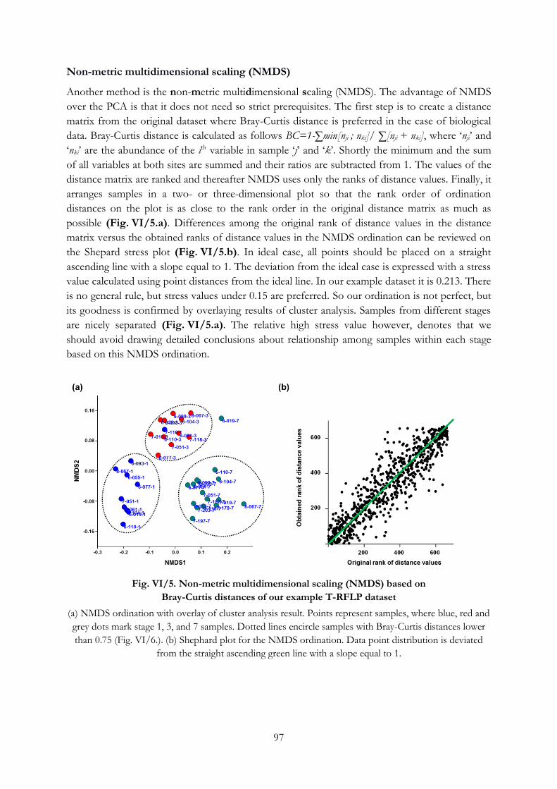
97
Non-metric multidimensional scaling (NMDS)
Another method is the non-metric multidimensional scaling (NMDS). The advantage of NMDS
over the PCA is that it does not need so strict prerequisites. The first step is to create a distance
matrix from the original dataset where Bray-Curtis distance is preferred in the case of biological
data. Bray-Curtis distance is calculated as follows BC=1-∑min[nji ; nki]/ ∑[nji + nki], where ‘nji’ and
‘nki’ are the abundance of the ith variable in sample ‘j’ and ‘k’. Shortly the minimum and the sum
of all variables at both sites are summed and their ratios are subtracted from 1. The values of the
distance matrix are ranked and thereafter NMDS uses only the ranks of distance values. Finally, it
arranges samples in a two- or three-dimensional plot so that the rank order of ordination
distances on the plot is as close to the rank order in the original distance matrix as much as
possible (Fig. VI/5.a). Differences among the original rank of distance values in the distance
matrix versus the obtained ranks of distance values in the NMDS ordination can be reviewed on
the Shepard stress plot (Fig. VI/5.b). In ideal case, all points should be placed on a straight
ascending line with a slope equal to 1. The deviation from the ideal case is expressed with a stress
value calculated using point distances from the ideal line. In our example dataset it is 0.213. There
is no general rule, but stress values under 0.15 are preferred. So our ordination is not perfect, but
its goodness is confirmed by overlaying results of cluster analysis. Samples from different stages
are nicely separated (Fig. VI/5.a). The relative high stress value however, denotes that we
should avoid drawing detailed conclusions about relationship among samples within each stage
based on this NMDS ordination.
Fig. VI/5. Non-metric multidimensional scaling (NMDS) based on
Bray-Curtis distances of our example T-RFLP dataset
(a) NMDS ordination with overlay of cluster analysis result. Points represent samples, where blue, red and
grey dots mark stage 1, 3, and 7 samples. Dotted lines encircle samples with Bray-Curtis distances lower
than 0.75 (Fig. VI/6.). (b) Shephard plot for the NMDS ordination. Data point distribution is deviated
from the straight ascending green line with a slope equal to 1.
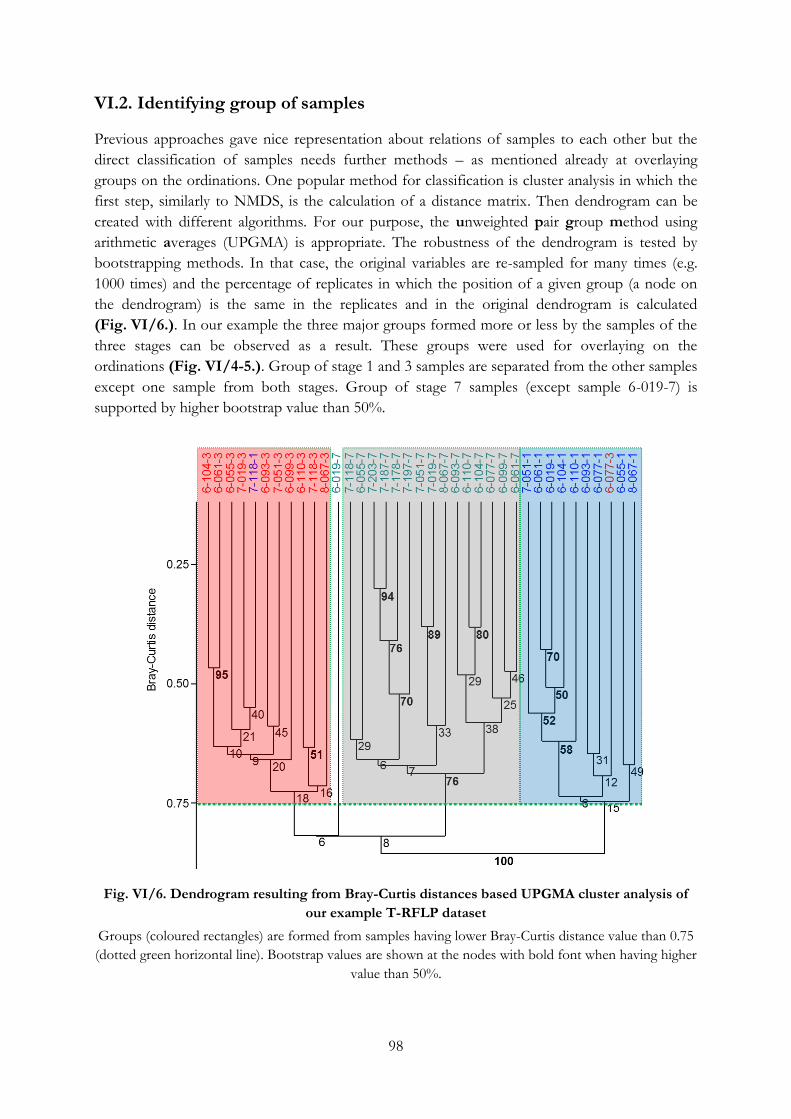
98
VI.2. Identifying group of samples
Previous approaches gave nice representation about relations of samples to each other but the
direct classification of samples needs further methods – as mentioned already at overlaying
groups on the ordinations. One popular method for classification is cluster analysis in which the
first step, similarly to NMDS, is the calculation of a distance matrix. Then dendrogram can be
created with different algorithms. For our purpose, the unweighted pair group method using
arithmetic averages (UPGMA) is appropriate. The robustness of the dendrogram is tested by
bootstrapping methods. In that case, the original variables are re-sampled for many times (e.g.
1000 times) and the percentage of replicates in which the position of a given group (a node on
the dendrogram) is the same in the replicates and in the original dendrogram is calculated
(Fig. VI/6.). In our example the three major groups formed more or less by the samples of the
three stages can be observed as a result. These groups were used for overlaying on the
ordinations (Fig. VI/4-5.). Group of stage 1 and 3 samples are separated from the other samples
except one sample from both stages. Group of stage 7 samples (except sample 6-019-7) is
supported by higher bootstrap value than 50%.
Fig. VI/6. Dendrogram resulting from Bray-Curtis distances based UPGMA cluster analysis of
our example T-RFLP dataset
Groups (coloured rectangles) are formed from samples having lower Bray-Curtis distance value than 0.75
(dotted green horizontal line). Bootstrap values are shown at the nodes with bold font when having higher
value than 50%.

99
VI.3. Hypothesis testing
Testing the separation of groups in multivariate dataset
Our example dataset consists of three main groups according to stage 1, 3 and 7 (that is the last
number of sample names). As we have already seen above the samples are separated according to
the stages. But the question is whether it is a statistically significant separation or not?
One way is to make a distance matrix among the samples and to tag distance values (Fig. VI/7.),
whether they represent the distances within one group (orange on the figure) or distances
between samples belong to different groups (green on the figure). We will end up in two lists of
distances which are plotted for better understanding. It shows that the range of distance values
overlaps in our example but the distance values are higher between groups than within groups.
Therefore our null hypothesis, what can be checked by two-sample t-test, is that ‘the means of
these two lists are the same’ (that is, means of the samples – within a group and between groups
– have the same distances from each other). The first step, in the evaluation of the test is to
define the null hypothesis. The second step, is to calculate the statistical p-value beside the truth
of the null hypothesis. In the case of the t-test it calculates the difference of means of the lists
and produce a probability value (p, which in our case is p = 1.7532 × 10-89). p value promotes to
reject or accept the null hypothesis: if p value is very low we make a small mistake if we reject the
null hypothesis, which denotes that the means of the two groups are quite different. We have to
note that variable thresholds (levels of significance, e.g. α < 0.01) are used for marking limit
under which p value is regarded as a statistically significant result. We always have to be aware
that at which level was the significance stated.
Fig. VI/7. Bray-Curtis distances among samples in our example dataset
The upper right triangle shows the distance matrix based on Bray-Curtis distances. Orange background
denotes within, while green background denotes between group distances. The two type of distance values
are plotted on the lower left graph.
Another analysis is the Anosim (analyis of similarity) which is based on similarities or distances
among samples (within and between groups as well). These values are converted to ranks to
compare the groups in a non-parametric statistical method. The null hypothesis is that ‘there are
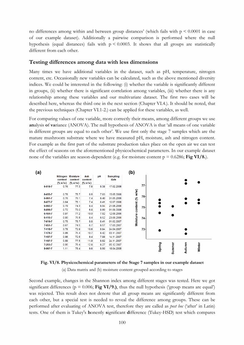
100
no differences among within and between group distances’ (which fails with p < 0.0001 in case
of our example dataset). Additionally a pairwise comparison is performed where the null
hypothesis (equal distances) fails with p < 0.0003. It shows that all groups are statistically
different from each other.
Testing differences among data with less dimensions
Many times we have additional variables in the dataset, such as pH, temperature, nitrogen
content, etc. Occasionally new variables can be calculated, such as the above mentioned diversity
indices. We could be interested in the following: (i) whether the variable is significantly different
in groups, (ii) whether there is significant correlation among variables, (iii) whether there is any
relationship among these variables and our multivariate dataset. The first two cases will be
described here, whereas the third one in the next section (Chapter VI.4.). It should be noted, that
the previous techniques (Chapter VI.1-2.) can be applied for these variables, as well.
For comparing values of one variable, more correctly their means, among different groups we use
analysis of variance (ANOVA). The null hypothesis of ANOVA is that ‘all means of one variable
in different groups are equal to each other’. We use first only the stage 7 samples which are the
mature mushroom substrate where we have measured pH, moisture, ash and nitrogen content.
For example as the first part of the substrate production takes place on the open air we can test
the effect of seasons on the aforementioned physicochemical parameters. In our example dataset
none of the variables are season-dependent (e.g. for moisture content p = 0.6286; Fig VI/8.).
Fig. VI/8. Physicochemical parameters of the Stage 7 samples in our example dataset
(a) Data matrix and (b) moisture content grouped according to stages
Second example, changes in the Shannon index among different stages was tested. Here we got
significant differences (p = 0.006; Fig VI/9.), thus the null hypothesis (‘group means are equal’)
was rejected. This result does not denote that all group means are significantly different from
each other, but a special test is needed to reveal the difference among groups. These can be
performed after evaluating of ANOVA test, therefore they are called as post hoc (‘after’ in Latin)
tests. One of them is Tukey's honestly significant difference (Tukey-HSD) test which compares
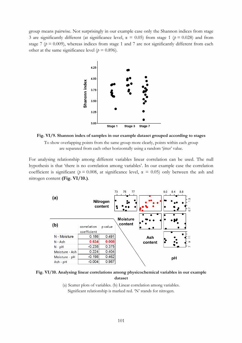
101
group means pairwise. Not surprisingly in our example case only the Shannon indices from stage
3 are significantly different (at significance level, α = 0.05) from stage 1 (p = 0.028) and from
stage 7 (p = 0.009), whereas indices from stage 1 and 7 are not significantly different from each
other at the same significance level (p = 0.896).
Fig. VI/9. Shannon index of samples in our example dataset grouped according to stages
To show overlapping points from the same group more clearly, points within each group
are separated from each other horizontally using a random ‘jitter’ value.
For analysing relationship among different variables linear correlation can be used. The null
hypothesis is that ‘there is no correlation among variables’. In our example case the correlation
coefficient is significant (p = 0.008, at significance level, α = 0.05) only between the ash and
nitrogen content (Fig. VI/10.).
Fig. VI/10. Analysing linear correlations among physicochemical variables in our example
dataset
(a) Scatter plots of variables. (b) Linear correlation among variables.
Significant relationship is marked red. ‘N’ stands for nitrogen.
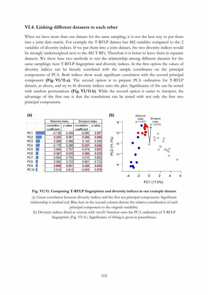
102
VI.4. Linking different datasets to each other
When we have more than one dataset for the same sampling, it is not the best way to put them
into a joint data matrix. For example the T-RFLP dataset has 482 variables compared to the 2
variables of diversity indices. If we put them into a joint dataset, the two diversity indices would
be strongly underweighted next to the 482 T-RFs. Therefore it is better to leave them in separate
datasets. We show here two methods to test the relationship among different datasets for the
same samplings: here T-RFLP fingerprints and diversity indices. In the first option the values of
diversity indices can be linearly correlated with the sample coordinates on the principal
components of PCA. Both indices show weak significant correlation with the second principal
component (Fig. VI/11.a). The second option is to prepare PCA ordination for T-RFLP
dataset, as above, and try to fit diversity indices onto the plot. Significance of fits can be tested
with random permutations (Fig. VI/11.b). While the second option is easier to interpret, the
advantage of the first one is that the correlations can be tested with not only the first two
principal components.
Fig. VI/11. Comparing T-RFLP fingerprints and diversity indices in our example dataset
(a) Linear correlation between diversity indices and the first ten principal components. Significant
relationship is marked red. Blue bars in the second column denote the relative contribution of each
principal component to the original variability.
(b) Diversity indices fitted as vectors with ‘envfit’ function onto the PCA ordination of T-RFLP
fingerprints (Fig. VI/4.). Significance of fitting is given in parentheses.
103
VII. SPECIES IDENTIFICATION IN PRACTICE (Erika
Tóth)
Systematics works with grouping, describing and nominating living organisms. There are three
separate but related disciplines in taxonomy:
Classification: groups living organisms into taxa based on their similarity and evolutionary
relationship
Nomenclature: nominates living organisms
Identification: places a given organism into an existing taxonomical group
In phenetic systems taxonomists group organisms based on mutual similarity of phenotypic
characteristics (numerical taxonomy). In phylogenetic systems groups are created based on shared
evolutionary relatedness.
In case of prokaryotes even to define the ‘species’ is not univoque:
A species at higher level eukaryotes is defined as the group of organisms capable of interbreeding
and producing fertile progeny, which is reproductively separated from other groups.
Bacteria of the same species must share many phenotypic properties – though many phenotypic
data are variable even within a species! Bacteria belonging to the same taxon must have similar
mol % G+C but two strains having the same mol % G+C are not necessarily belonging to the
same species. The DNA from organisms of the same species should show a minimum of 70%
reassociation (total genome DNA-DNA hybridisation value). Moreover 16S rRNA gene
sequence similarity between the two strains should be above 98% in case they belong to the same
species (but there are also some exceptions!). Describing a novel taxon in microbiology must be
done on a polyphasic approach - which means complete phenotypic characterisation (including
chemotaxonomy) and also genotypic studies.
Characters to be studied in case of description a novel taxon:
1. Phenotypic characters
Cell and colony morphology - light microscope and TEM (Transmission Electron
Microscopy) (cell size, shape, cell cycle, heterocyst, etc.); appearance in liquid culture, on
solid medium (colour, colony size, elevation, shape, consistency, mycelium production,
etc.), motility (flagellation type), presence of endospores, capsule, inclusions, etc.
Staining properties (Gram staining, acid fast staining, endospore staining, etc.)
Physiological characteristics (temperature, pH tolerance, ecophysiological markers,
pathogenicity, etc.)
Biochemical properties (enzyme reactions - classical tests and fast kits)
Complete chemotaxonomy (cell wall type, lipoquinones, fatty acids, polar lipid profiles,
MALDI-TOF MS, etc.)
Immunological characterisation (when necessary)
2. Nucleic acid studies
Determination of the G+C content of DNA
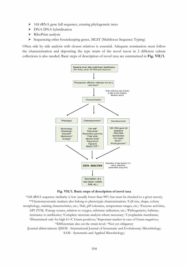
104
16S rRNA gene full sequence, creating phylogenetic trees
DNA-DNA hybridisation
RiboPrint analysis
Sequencing other housekeeping genes, MLST (Multilocus Sequence Typing)
Often side by side analysis with closest relatives is essential. Adequate nomination must follow
the characterisation and depositing the type strain of the novel taxon in 2 different culture
collections is also needed. Basic steps of description of novel taxa are summarized in Fig. VII/1.
Fig. VII/1. Basic steps of description of novel taxa
*16S rRNA sequence similarity is low (usually lower than 98% but must be checked to a given taxon);
**Chemotaxonomic markers also belong to phenotypic characterisation; 1Cell size, shape, colony
morphology, staining characteristics, etc.; 2Salt, pH tolerance, temperature ranges, etc.; 3Enzyme activities,
API ZYM; 4Energy source, relation to oxygen, substrate utilisation, etc.; 5Pathogenicity, habitats,
resistance to antibiotics; 6Complete structure analysis where necessary; 7Cytoplasmic membrane; 8Determined only for high G+C Gram-positives; 9Important marker in case of Gram-negatives;
10Differentiate also on the strain level; 12Not yet obligatory
(Journal abbreviations: IJSEM - International Journal of Systematic and Evolutionary Microbiology;
SAM - Systematic and Applied Microbiology)
105
Source of figures
Adapted from Tóth and Márialigeti, 2013: III/1-4., IV/5-7., IV/14.
Attila Szabó: IV/2., IV/9-12.
Balázs Vajna: IV/1., IV/3-4., IV/13., IV/17., IV/19., VI/1-11.
Erika Tóth: II/1., II/4-5., III/8., V/1-3., VII/1.
Judit Makk and Erika Tóth: II/3.
Judit Makk: II/2.
Márta Vargha: III/6-7.
Rita Sipos: IV/16., IV/18.
Sauer and Kliem, 2010: III/5.
Six et al., 2007: IV/15.a
Tamás Felföldi: IV/8., IV/15.b, IV/21., IV/22.
Tamás Felföldi and Balázs Vajna: cover
Zsuzsanna Pohner: IV/20.
106
References
Borsodi, A., Felföldi, T., Jáger, K., Makk, J., Márialigeti, K. (Ed), Romsics, Cs., Tóth, E., Bánfi,
R., Pohner, Zs., Vajna, B. 2013. ‘Bevezetés a prokarióták világába’ (Introduction to the world
of prokaryotes). ELTE, Budapest
http://www.eltereader.hu/media/2014/04/Bevezetes_a_prokariotak_vilagaba.pdf
Garthright, W.E., Blodgett, R.J., 2003. FDA’s preferred MPN methods for standard, large or
unusual tests, with a spreadsheet. Food Microbiology 20, 439-445.
Goodfellow, M., Sutcliffe, I., Chun J. (Eds.) 2014. New Approaches to Prokaryotic Systematics.
Methods in Microbiology, Volume 41. Academic Press, London.
Rainey, F., Oren, A. (Eds.) 2014. Taxonomy of Prokaryotes. Methods in Microbiology, Volume
38. Academic Press, London.
Sauer, S., Kliem, M. 2010. Mass spectrometry tools for the classification and identification of
bacteria. Nature Reviews Microbiology 8, 74-82.
Six, C., Thomas, J.C., Garczarek, L., Ostrowski, M., Dufresne, A., Blot, N., Scanlan, D.J.,
Partensky, F. 2007. Diversity and evolution of phycobilisomes in marine Synechococcus spp.: a
comparative genomics study. Genome Biology 8, R259.
Tóth, E.M., Márialigeti, K. (Eds.) 2013. Practical Microbiology, ELTE, Budapest
http://www.eltereader.hu/media/2014/05/Practical_microbiology_READER.pdf
Vajna, B., Szili, D., Nagy, A., Márialigeti, K. 2012. An improved sequence aided T-RFLP analysis
of bacterial succession during oyster mushroom substrate preparation. Microbial Ecology,
64, 702-713.