Metode şi Algoritmi de Planificareandrei.clubcisco.ro/cursuri/5master/g-map/12_AplicatiiMAP.pdfUniversitatea Politehnica Bucureşti - Facultatea de Automatica si Calculatoare Scheduling

Universitatea Politehnica Bucureşti - Facultatea de Automatica si Calculatoare

1

Metode şi Algoritmi de Planificare

(MAP)

2009-2010

Curs 12

Aplicaţii ale algoritmilor şi metodelor de

planificare

12.01.2010 Metode si Algoritmi de Planificare – Curs 12


Application of Scheduling

• Exam Timetabling

• Traveling Salesman Problem

• Sports Scheduling

– An Assessment of Various Approaches to Solving the n-Round

Robin Tournament

• Employee Scheduling

• Car Sequencing

• Job-Shop Scheduling

12.01.2010 Metode si Algoritmi de Planificare – Curs 12 2


Scheduling problem

• Scheduling is the allocation, subject to constraints, of resources to objects being placed in space-time, in such a way as to minimize the total cost of some set of the resources used.

• Sequencing is the construction, subject to constraints, of an order in which activities are to be carried out or objects to be placed in some representation of a solution.

Examples: – traveling salesman problem,

– car sequencing.



EXAM TIMETABLING



5

EXAM TIMETABLING

• The problem can be defined as assigning a set

of examinations to a fixed number of time

periods so that no student is required to take

more than one examination at any time.

• There are two tasks:

– Exam time period assignment

– Room assignment



6

Requirements• Exams

– All student groups taking the same exam must be arranged to sit the exam at the same time. (hard)

– Some specific exams should be assigned to a fixed date or a fixed time interval. (soft)

• Time periods

– Students can not attend several exams at a time. (hard)

– Release date or due date of an exam may be predetermined. (soft)

– One exam is not allowed to elapse more than a haft day. (hard)

• Rooms

– When there are several student groups taking the same exam, rooms for that exam should be arranged near to one another. (soft)

– Not more than 2 exams can be assigned to the same room. (hard)

– The rooms are assigned to exams in order that we can maximum the room utilization, i.e. we want to minimize the room waste. (soft)

– Each student’s exams should be spread over the exam season. (soft)



7

Problem Formulation

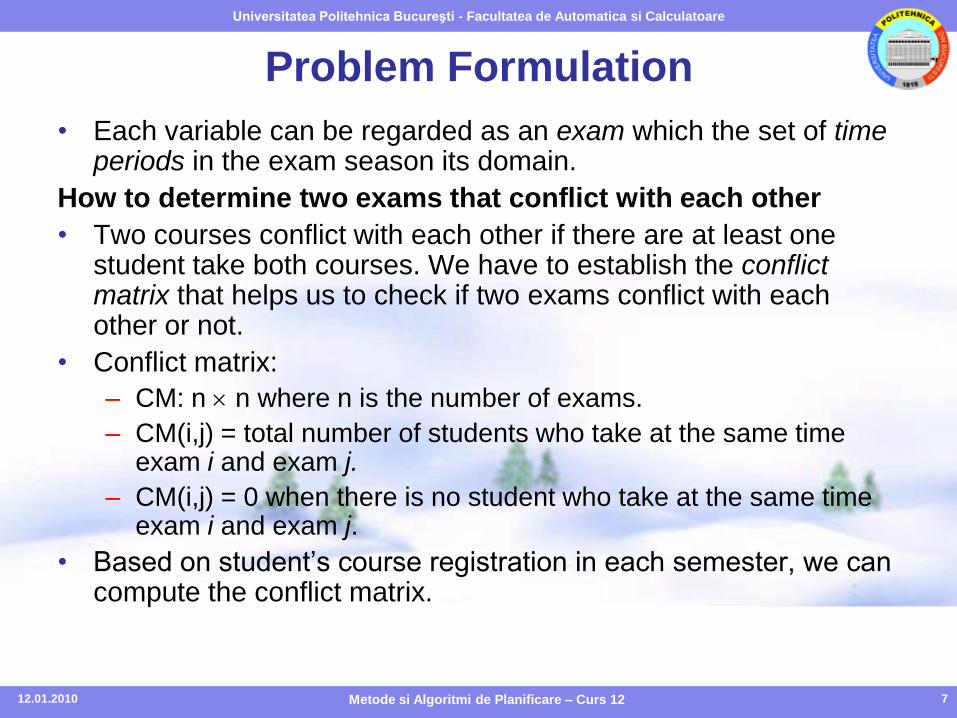
• Each variable can be regarded as an exam which the set of time periods in the exam season its domain.

How to determine two exams that conflict with each other

• Two courses conflict with each other if there are at least one student take both courses. We have to establish the conflict matrix that helps us to check if two exams conflict with each other or not.

• Conflict matrix:

– CM: n n where n is the number of exams.

– CM(i,j) = total number of students who take at the same time exam i and exam j.

– CM(i,j) = 0 when there is no student who take at the same time exam i and exam j.

• Based on student’s course registration in each semester, we can compute the conflict matrix.



8

Solving Method

• The approach we take to the exam timetabling problem consists of two stages:

– 1. Backtracking with Forward Checking (BC-FC) algorithm: to obtain an initial feasible timetable.

– 2. A Local Search algorithm (Tabu search or Simulated Annealing) : to improve the quality of the timetable.

• The first stage is used to obtain an initial schedule satisfying all the hard constraints.

• The second stage aims to improve the quality of the schedule, taking the soft constraints into account. The method used in the second stage is optimization method, which will seek to minimize a given objective function (the cost function).



9

Phase I (Generating Initial Feasible

Solution)

• The Backtracking with Forward Checking algorithm (BC-FC) is used to generate an initial feasible solution.

• In BC-FC, the variable ordering heuristic is based on the degrees of difficulty of the exams. This degree of difficulty is defined as follow:

markFail = x domainSize / markDomain + y markConflict + z markStudent

domainSize: number of legal timeslots to which the remaining exams can be assigned.

markDomain: number of legal timeslots to which the current exam can be assigned

markConflict: number of exams to which the current exam is conflicting

markStudent: number of students that attend the current exam

x, y, z : the parameters will be defined

• The most difficult exam will have the highest priority to be selected.

• In BC-FC, we also use value-ordering heuristic which bases on the cost function that helps to spread the student’s exams over the exam season.



10

Phase II ( Local search Algorithm)

• In this phase, we can use a Tabu Search or Simulated Annealing algorithm. We can also use Min-conflict Hill Climbing or WSAT algorithm.

Atomic Move and Neighborhood

• Let a solution s = (S1, S2,…, Sn), where Si is the set of exams assigned to timeslot Ti. An atomic move is one such that exactly an exam x is moved from a timeslot Ti to another timeslot Tj, denoted as (x, i, j). We call s’ is a neighbor of s and all the neighbors generated from s by an atomic move as the neighborhood of s.



11

Cost Function

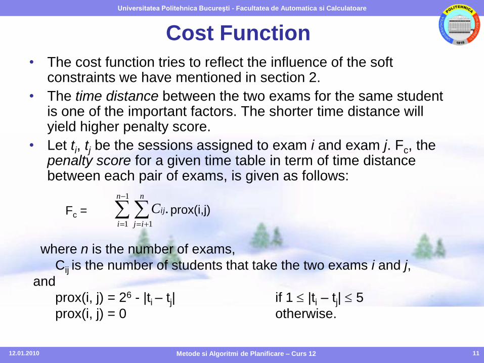
• The cost function tries to reflect the influence of the soft constraints we have mentioned in section 2.

• The time distance between the two exams for the same student is one of the important factors. The shorter time distance will yield higher penalty score.

• Let ti, tj be the sessions assigned to exam i and exam j. Fc, the penalty score for a given time table in term of time distance between each pair of exams, is given as follows:

1

1 1

.n

i

n

ij

ijCFc = prox(i,j)

where n is the number of exams,

Cij is the number of students that take the two exams i and j,

and

prox(i, j) = 26 - |ti – tj| if 1 |ti – tj| 5

prox(i, j) = 0 otherwise.



12

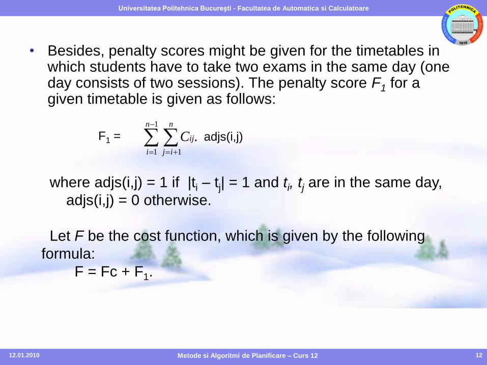
• Besides, penalty scores might be given for the timetables in which students have to take two exams in the same day (one day consists of two sessions). The penalty score F1 for a given timetable is given as follows:

1

1 1

.n

i

n

ij

ijCF1 = adjs(i,j)

where adjs(i,j) = 1 if |ti – tj| = 1 and ti, tj are in the same day,

adjs(i,j) = 0 otherwise.

Let F be the cost function, which is given by the following

formula:

F = Fc + F1.



13

Room Assignment

• One approach is similar to best-fit method:

For each exam period, sort the available rooms in

descending order by capacity; sort the examinations in

descending order by number of students. The largest

exam is assigned to the smallest room with sufficient

capacity to hold the students. If no room is large enough,

then the largest room is filled and remaining students are

assigned to a different.



TRAVELING SALESMAN

PROBLEM



15

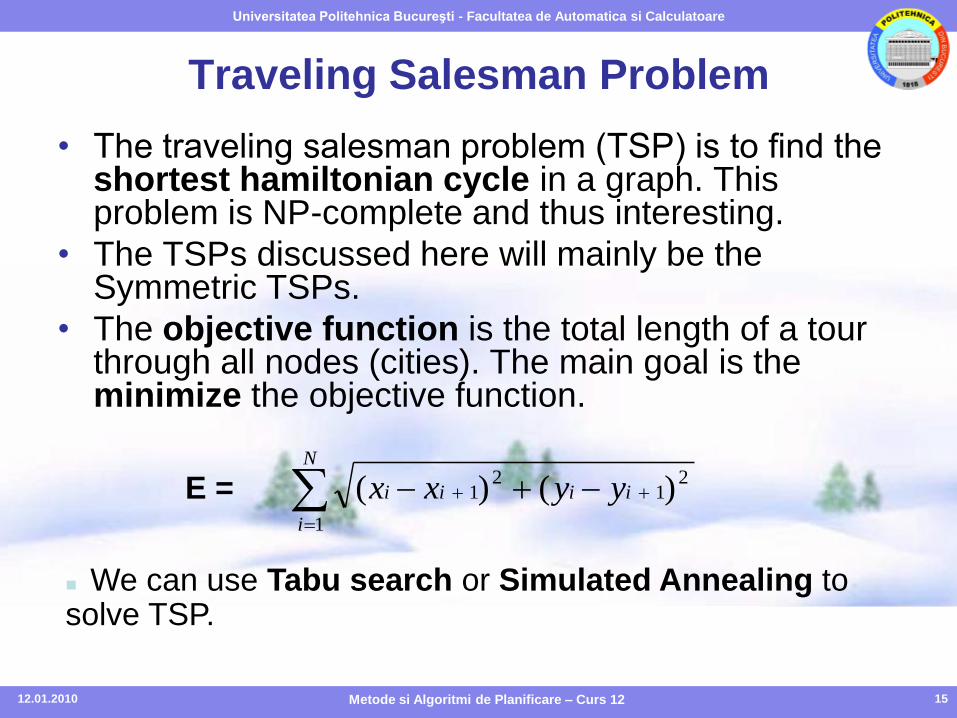
Traveling Salesman Problem

• The traveling salesman problem (TSP) is to find the shortest hamiltonian cycle in a graph. This problem is NP-complete and thus interesting.

• The TSPs discussed here will mainly be the Symmetric TSPs.

• The objective function is the total length of a tour through all nodes (cities). The main goal is the minimize the objective function.

We can use Tabu search or Simulated Annealing to solve TSP.

N

i

iiii yyxx1

21

21 )()(E =



16

How to create initial tour

• There are some tour construction algorithms. The best tour construction algorithms can get within 10-15% of optimality.

• One of the tour construction algorithm: nearest neighbor algorithm.

• Nearest neighbor– 1.Select a random city.

– 2. Find the nearest unvisited city and go there.

– 3. Are there any unvisitied cities left? If yes,

repeat step 2.

– 4. Return to the first city.

• Complexity of nearest neighbor algorithm: O(n)



17

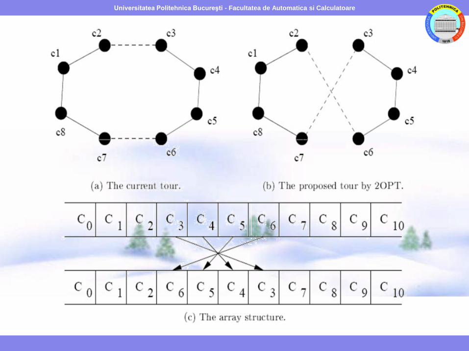
2-opt Move

• Once a tour has been generated by some tour

construction heuristic, we might wish to improve that

solution. There are several ways to do this, but the most

common one is the 2-opt move.

• The 2-opt move basically removes two edges from the

tour, and reconnects the two paths created. There is

only one way to reconnect the two paths so that we still

have a valid tour. We do this only if the new tour will be

shorter.

• Simulated Annealing and Tabu search can use 2-opt

moves to find neighboring solutions.





19

Tabu search for TSP

• Neighborhood operator: 2-opt move.

• After moving to a neighbor solution the move will be put on the tabu-list.

• There are several ways of implementing the tabu list. – One involves adding the two edges being removed by a 2-

opt move to the list. A move will then be considered tabu if it tries to add the same pair of edges again.

– Another way is to add the shortest edge removed by a 2-opt move, and then making any move involving this edge tabu.



20

Simulated Annealing for TSP

• Neighborhood operator: 2-opt move

• Initial Temperature: 10% of the cost of the initial tour (5% of the cost of a randomly generated initial tour.)

• Final Temperature: 0.000001

• Temperature reduction factor: = 0.99



21

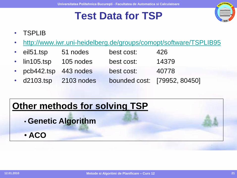
Test Data for TSP

• TSPLIB

• http://www.iwr.uni-heidelberg.de/groups/comopt/software/TSPLIB95

• eil51.tsp 51 nodes best cost: 426

• lin105.tsp 105 nodes best cost: 14379

• pcb442.tsp 443 nodes best cost: 40778

• d2103.tsp 2103 nodes bounded cost: [79952, 80450]

Other methods for solving TSP

• Genetic Algorithm

• ACO


http://www.iwr.uni-heidelberg.de/groups/comopt/software/TSPLIB95




SPORT SCHEDULING



Sports Scheduling

• Scheduling tournaments in a sports league

• Focusing on Round Robin Tournaments

– Single Round Robin Tournament (SRRT): each team meets every

other team once

– Double Round Robin Tournament (DRRT): each team meets

every other team twice

• Economic impact: quality of schedule affects the revenue of the

sports team

12.01.2010 23Metode si Algoritmi de Planificare – Curs 12


What is the best schedule?

• Home-away pattern– Balance between number of home and away games

– Prefer alternating home away pattern

• Any deviation is considered a break

• Minimizing Distance Travelled

• Other factors:– Availability of stadium

– Preferences to increase revenues

– Top team and bottom team constraints

– Geographical constraints



Main Considerations

• Minimizing number of breaks

– Used when teams return home after each away game instead of

travelling to another away game

– Alternating patterns usually preferred

– Considers the fans

– Ensures regular earnings from home games

• Minimizing distance travelled

– Used when teams travel to multiple away games without returning

home

– Huge savings can be obtained



Minimizing Number of Breaks

• Graph theoretical approaches

– 1-factorization: partitioning the games into n-1 slots, each node

will be incident to exactly one edge in each 1-factor

• Practical applications: constrained minimum break

problem

– Decomposition approach

– Combinatorial design, IP, enumeration techniques

– See Nemhauser and Trick

– Constraint programming approaches; see Henz



Minimizing Distance Travelled

• Similar to a travelling salesman problem

• Problem is too large to solve using IP in a reasonable amount

of time

• Various heuristics used instead

• The travelling tournament problem proposed by Easton,

Nemhauser, and Trick



The Travelling Tournament Problem

• Double round robin tournament to be played by n teams

over (2n-2) periods or weeks, where each team plays

every period

• Objective: minimize distance travelled by each team

• Additional Constraints:

– Maximum “road trip” of three games

– Maximum “home stand” of three games

– Repeater rule



TTP Solution Approaches

• What Methods Can We Use to Solve the TTP?

– Integer programming

– Constraint programming

– Hybrid approaches involving heuristics



A Tiling Approach for Fast

Implementation of the TTP

• Model the road trips as “tiles”

• Each tile will contain “blocks”, which represent individual

games

– (i.e. – a road trip with 3 opponents is considered as one tile, with 3

blocks)

• Three phase approach:

– Phase I – Tile Creation

– Phase II – Tile Placement

– Phase III – Block Placement



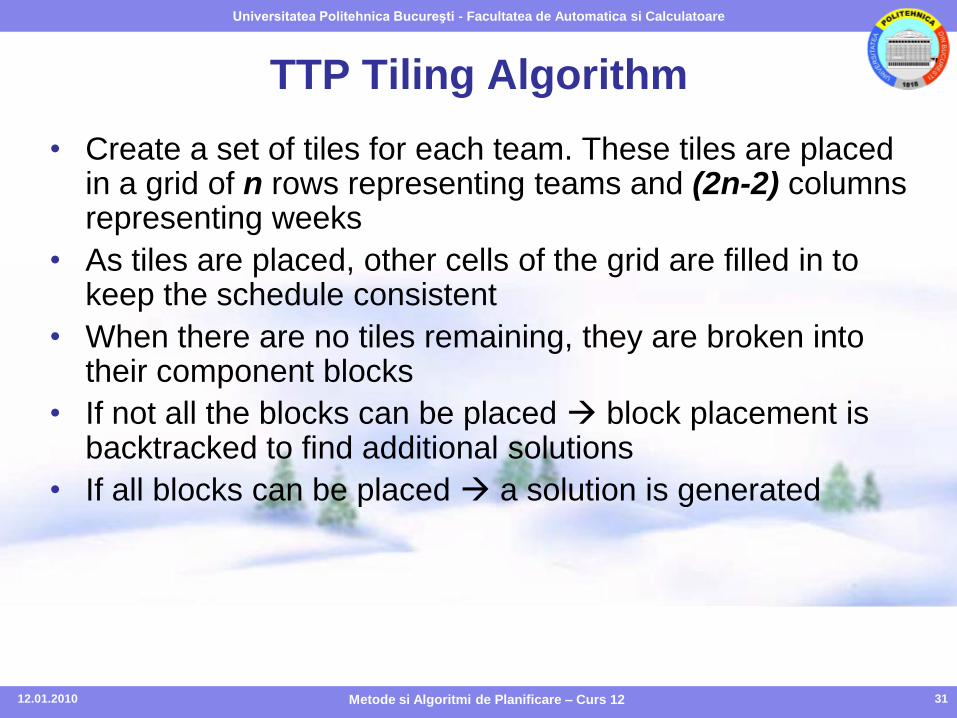
TTP Tiling Algorithm

• Create a set of tiles for each team. These tiles are placed in a grid of n rows representing teams and (2n-2) columns representing weeks

• As tiles are placed, other cells of the grid are filled in to keep the schedule consistent

• When there are no tiles remaining, they are broken into their component blocks

• If not all the blocks can be placed block placement is backtracked to find additional solutions

• If all blocks can be placed a solution is generated



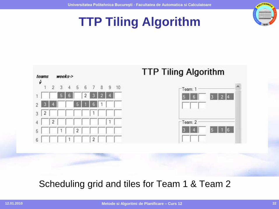
TTP Tiling Algorithm

Scheduling grid and tiles for Team 1 & Team 2



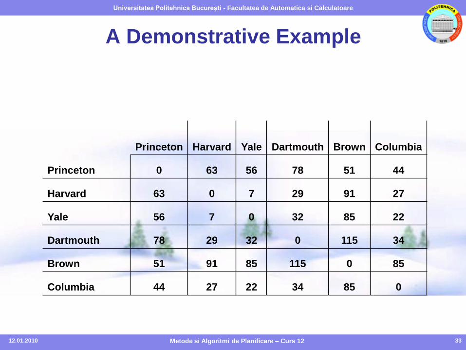
A Demonstrative Example

Princeton Harvard Yale Dartmouth Brown Columbia

Princeton 0 63 56 78 51 44

Harvard 63 0 7 29 91 27

Yale 56 7 0 32 85 22

Dartmouth 78 29 32 0 115 34

Brown 51 91 85 115 0 85

Columbia 44 27 22 34 85 0



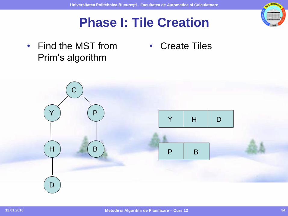
• Create Tiles

Phase I: Tile Creation

• Find the MST from

Prim’s algorithm

C

P

B

Y

H

D

Y H D

BP



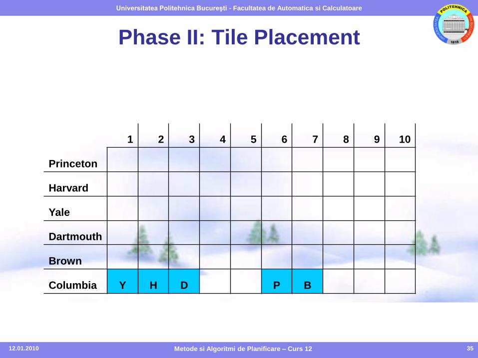
Phase II: Tile Placement

1 2 3 4 5 6 7 8 9 10

Princeton

Harvard

Yale

Dartmouth

Brown

Columbia Y H D P B



Phase III: Block Placement

• All remaining unplaced tiles are broken into individual blocks

• These blocks are placed into the scheduling grid

• Backtracking is used when blocks do not lead to a solution



Sports Scheduling - Conclusions

• Sports scheduling has huge economic implications for the sports industry

• Optimal solutions that consider the many constraints are time consuming

• Hybrid solutions involving heuristics are close to optimality and require less time

• Many opportunities for further research, particularly involving hybrid approaches



EMPLOYEE SCHEDULING



39

EMPLOYEE SCHEDULING

• In employee scheduling problem (ETP), we are given – a set of employees with various qualifications, pay-rates

and availabilities.

– a set of shifts with skill requirements and known start and end times.

• The objective is to assign an employee to every shift during a time period such that the constraints are satisfied and the schedule’s cost is minimized.

• Example: Timetabling nurses in a department (ward) in a hospital.



40

Example: Nurse Timetabling

• The nurses in a ward are of several types and they can be assigned to different roles in several types of shifts. Usually there are three shifts per day: morning, evening, and night.

• Timetabling period can be 2 weeks or a month.

• Each nurse has a list of preferred shifts for each week and a list of forbidden shifts, due to her personal wishes.

• Usually nurses have some limit on the total number of hours or shifts they are allowed to work, and some constraints such as: not working more than two consecutive nights.

• In addition, there are some global constraints, e.g. distributing night shifts equally among all nurses or distributing weekend shifts equally over a long period.



41

The Constraints

There are several kinds of constraints in the employee scheduling problem:

• (1) Employee Clashing Constraints: An employee can not be assigned to two shifts at the same time, or be assigned during a time when the employee is not available.

• (2) Qualification Constraints: this constraint is violated if an employee is assigned to a shift for which the shift’s requirements are not a subset of the employee’s qualifications.

• (3) Exclusion Constraints: this constraint is violated if an employee is assigned to a shift that he or she should be excluded from.

• (4) Personnel requests are requirements given by the employees. These are mostly wishes to have some days off.

Constraints of types (1), (2), (3) are hard constraints and must be satisfied. The constraints of type (4) are soft constraints.



42

The Objective Function

We use a multi-criteria objective function that involves the objectives described below.

• Labor cost and overtime: Overtime is calculated as follows:

– An employee’s week is split into a sequence of “logical” days. A logical day is a sequence of shifts where there is less than 8 hours rest between each shift.

– An employee accrues daily overtime for the amount of work in each logical day that exceeds 8 hours. The daily overtime is the sum of the overtime for every logical day.

– An employee accrues weekly overtime for the amount work in a week that exceed 40 hours minus the amount of daily overtime.

– An employee is paid for overtime at a rate that is 1.5 times their regular salary.

• Training costs: Training costs occur when an employee is booked for a shift associated with a job that they have not worked before. In such cases, the training cost is calculated as the duration of the shift times the employee’s pay rate.



43

The Objective Function (cont.)

• Fairness: Fairness measures how well the work is spread amongst the employees. An employee’s requested number of hours per week is used as the basis for modeling fairness.

• Notice that labor law constraints ( for example, an employee can work two consecutive days with less than 8 hours rest) are not modeled explicitly but are implicit in the calculation of overtime.

• We place the highest priority on satisfying the hard constraints, then trying to satisfy the soft constraints, and finally considering a weighted sum of the other costs.



44

Problem Representation

• The main representation of ETPs has employees as

variables and shifts as values to be assigned to

variables.

– Each employee can be represented by a number of

variables, that stand for the number of shifts that the

employee can be assigned in the timetabling period.

• Note: In the dual representation, we can also regard

shifts as variables and employees as values.



45

Problem Representation (cont)

• Example: In nurse scheduling problem, there is a variable for each nurse on a day. The domains of the variables consists of possible shifts, i.e. D = {0,1,2,3}. For a nurse i and a day j a variable vij may have one of the following values:

vij=0 : the nurse i is off-duty on the day j

vij=1 : the nurse i takes the “morning” shift on the day j

vij=2 : the nurse i takes the “evening” shift on the day j

vij=3 : the nurse i take the “night” shift on the day j

• Let see a problem with 20 nurses in 30 days using 3-shift model. There are 600 variables involved.



46

Solving Methods

Method 1.

• Since ETP is an constraint optimization satisfaction problem, and an over-constrained system consisting of hard and soft constraints, we can formulate it as a PCSP and use Branch&Bound with forward checking algorithm with some domain specific heuristics to solve it.

• Experience shows that these domain-specific heuristics (variable ordering, value ordering, constraint ordering) are crucial in helping to accelerate the search.

Method 2.

• We can use a greedy algorithm to generate an initial solution and then apply some iterated local search method (e.g., tabu search) to improve repeatedly the quality of the solution.



CAR SEQUENCING



48

CAR SEQUENCING

• Cars in productions are placed on an assembly line that moves through various production units responsible for installing such options as air-conditioning, radios, etc.

• The assembly line can be viewed as composed of slots, and each car must be allocated to a single slot.

• The production units have limited capacity and they need time to set up the options on the car as the assembly line is moving. These capacity constraints are of the form r out of s.

• The unit is able to produce at most r cars with the option out of each sequence of s cars.

• The car sequencing problem aims to find an assignment of cars to the slots that satisfied the capacity constraints.



49

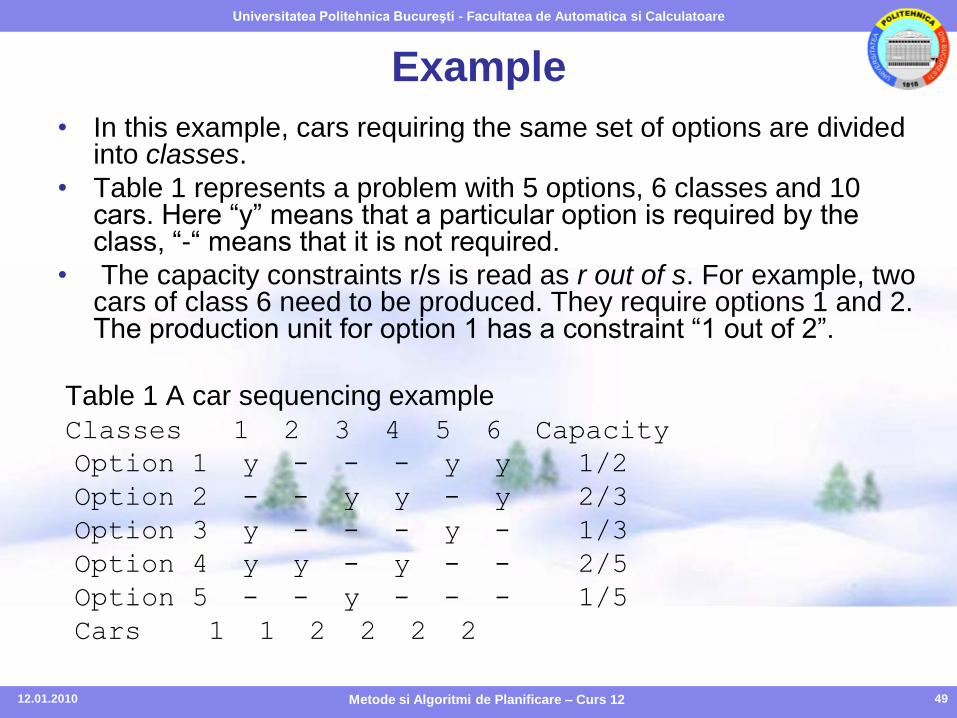
Example

• In this example, cars requiring the same set of options are divided into classes.

• Table 1 represents a problem with 5 options, 6 classes and 10 cars. Here “y” means that a particular option is required by the class, “-“ means that it is not required.

• The capacity constraints r/s is read as r out of s. For example, two cars of class 6 need to be produced. They require options 1 and 2. The production unit for option 1 has a constraint “1 out of 2”.

Table 1 A car sequencing example

Classes 1 2 3 4 5 6 Capacity

Option 1 y - - - y y 1/2

Option 2 - - y y - y 2/3

Option 3 y - - - y - 1/3

Option 4 y y - y - - 2/5

Option 5 - - y - - - 1/5

Cars 1 1 2 2 2 2



50

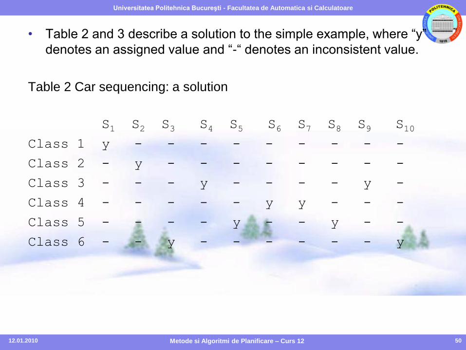
• Table 2 and 3 describe a solution to the simple example, where “y”

denotes an assigned value and “-“ denotes an inconsistent value.

Table 2 Car sequencing: a solution

S1 S2 S3 S4 S5 S6 S7 S8 S9 S10

Class 1 y - - - - - - - - -

Class 2 - y - - - - - - - -

Class 3 - - - y - - - - y -

Class 4 - - - - - y y - - -

Class 5 - - - - y - - y - -

Class 6 - - y - - - - - - y



51

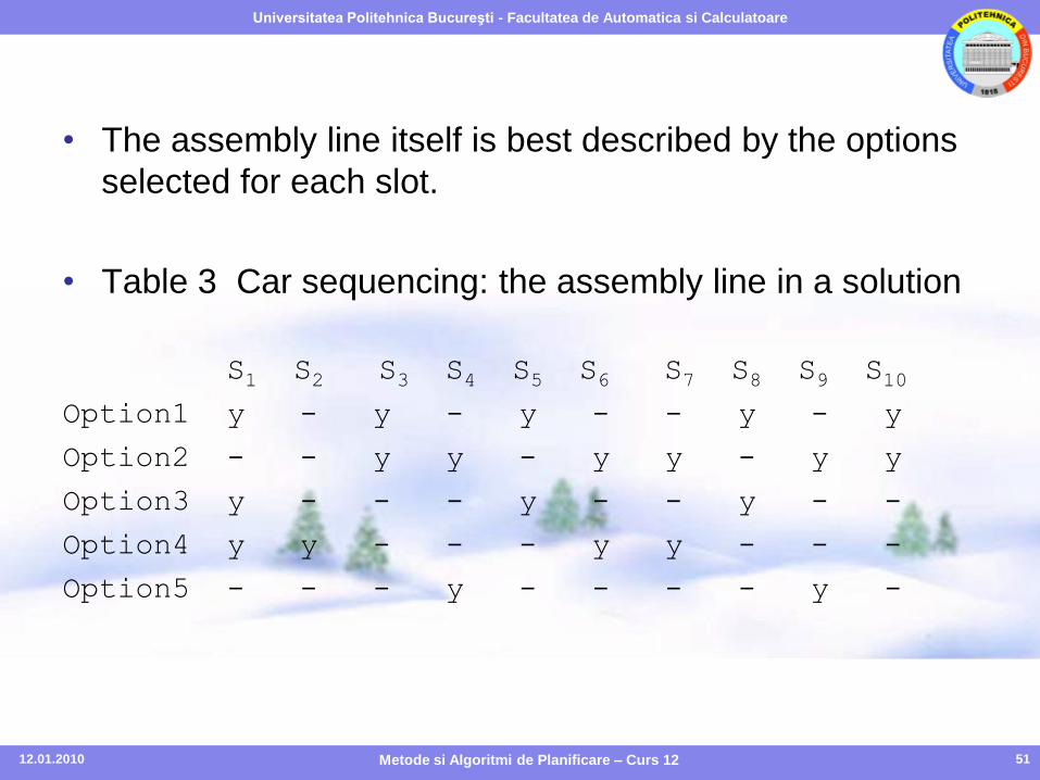
• The assembly line itself is best described by the options

selected for each slot.

• Table 3 Car sequencing: the assembly line in a solution

S1 S2 S3 S4 S5 S6 S7 S8 S9 S10

Option1 y - y - y - - y - y

Option2 - - y y - y y - y y

Option3 y - - - y - - y - -

Option4 y y - - - y y - - -

Option5 - - - y - - - - y -



52

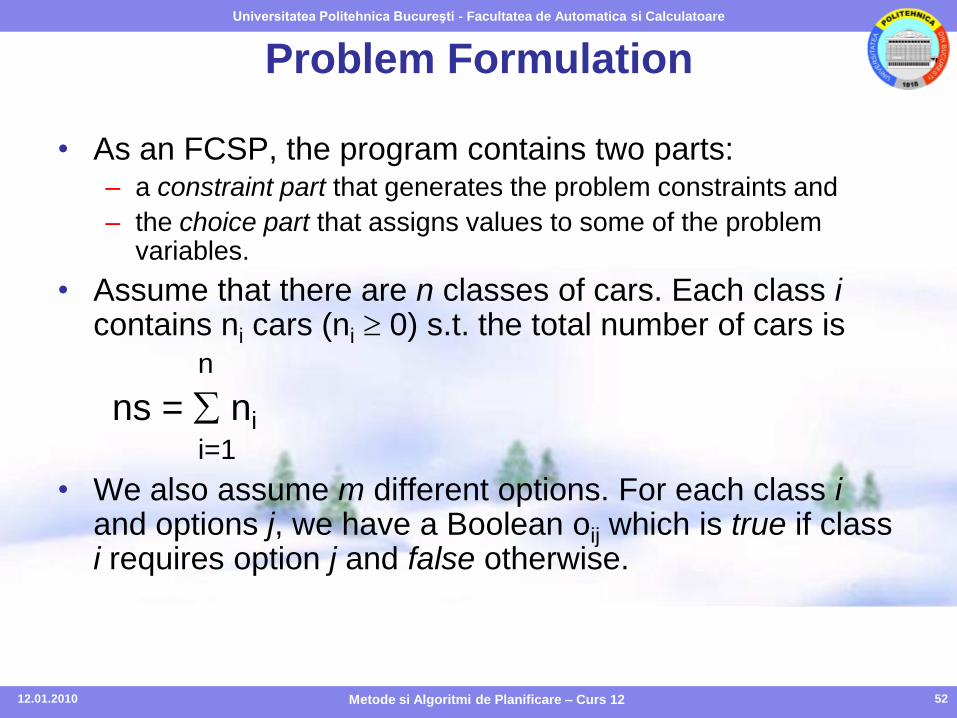
Problem Formulation

• As an FCSP, the program contains two parts:– a constraint part that generates the problem constraints and

– the choice part that assigns values to some of the problem variables.

• Assume that there are n classes of cars. Each class icontains ni cars (ni 0) s.t. the total number of cars is

n

ns = ni

i=1

• We also assume m different options. For each class iand options j, we have a Boolean oij which is true if class i requires option j and false otherwise.



53

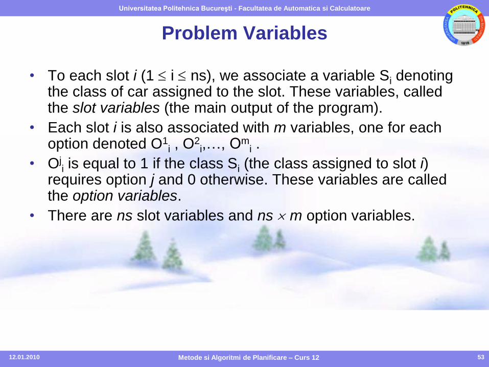
Problem Variables

• To each slot i (1 i ns), we associate a variable Si denoting the class of car assigned to the slot. These variables, called the slot variables (the main output of the program).

• Each slot i is also associated with m variables, one for each option denoted O1

i , O2i,…, Om

i .

• Oji is equal to 1 if the class Si (the class assigned to slot i)

requires option j and 0 otherwise. These variables are called the option variables.

• There are ns slot variables and ns m option variables.



54

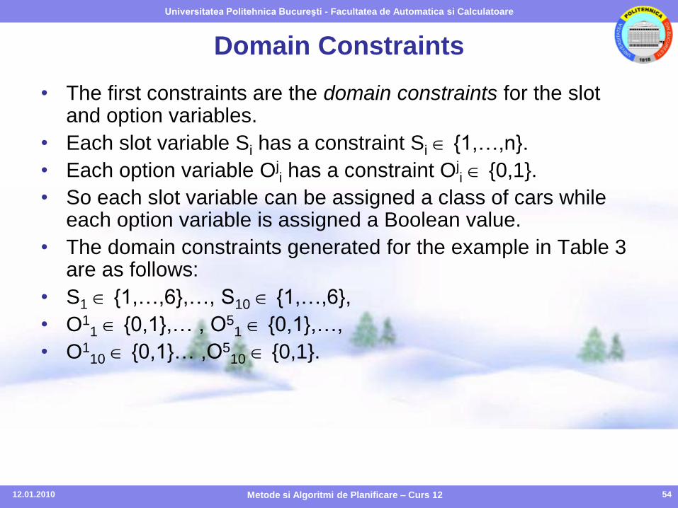
Domain Constraints

• The first constraints are the domain constraints for the slot and option variables.

• Each slot variable Si has a constraint Si {1,…,n}.

• Each option variable Oji has a constraint Oj

i {0,1}.

• So each slot variable can be assigned a class of cars while each option variable is assigned a Boolean value.

• The domain constraints generated for the example in Table 3 are as follows:

• S1 {1,…,6},…, S10 {1,…,6},

• O11 {0,1},… , O5

1 {0,1},…,

• O110 {0,1}… ,O5

10 {0,1}.



55

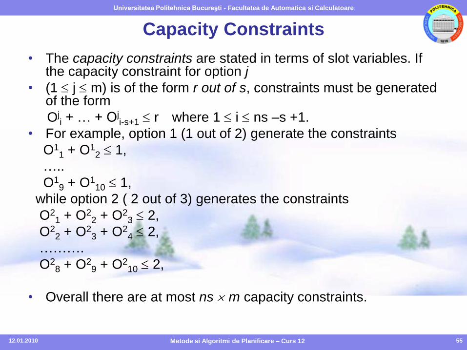
Capacity Constraints

• The capacity constraints are stated in terms of slot variables. If the capacity constraint for option j

• (1 j m) is of the form r out of s, constraints must be generated of the form

Oji + … + Oj

i-s+1 r where 1 i ns –s +1.

• For example, option 1 (1 out of 2) generate the constraints

O11 + O1

2 1,

…..

O19 + O1

10 1,

while option 2 ( 2 out of 3) generates the constraints

O21 + O2

2 + O23 2,

O22 + O2

3 + O24 2,

……….

O28 + O2

9 + O210 2,

• Overall there are at most ns m capacity constraints.



56

Demand Constraints

• It is also necessary to make sure that the cars requested are produced.

• For each class i (1 i n), we have to generate a constraint

exactly(ni, [S1,…,Sns],i)

where S1,…,Sns are slot variables and ni is the number of cars in class i.

• The constraint exactly(N, L, M) holds true iff there are exactly N variables in the list L whose values are equal to M.

• Since there are ns slot variables and each of them will be assigned to a class, we only need to make sure that the assignment produces no more cars from a class than are actually necessary.

• So we rewrite the above constraints as

atmost(ni, [S1,…,Sns],i)

The constraint atmost(N,L, M) holds true iff there are at most N variables in the list L whose values are equal to M.



57

Link Constraints

• These constraints links option variables and slot variables together.

• For all i, j: if Si is assigned the value k, the Oji = 1 if class k

requires option j, 0 otherwise.

• The link is achieved by producing constrains of the form element(I, L, V) which holds true iff element I of the list L is equal to V.

• Each option j will be connected with slot i by the constraint

• element(Si, [o1j, …,onj], Oji )

• where o1j, …,onj are the 0-1 values specifying which classes require option j.



58

Link Constraints (cont.)

• In the example, the connection between the slots and options is enforced by the constraints:

element(S1, [1,0,0,0,1,1], O11),

…………

element(S1, [0,0,1,0,0,0], O51),

…………

element(S10, [1,0,0,0,1,1], O110 ),

……..

element(S10, [0,0,1,0,0,0], O510 ).

• There are ns m link constraints.



59

Redundant Constraints

• Redundant constraints are constraints which are not strictly necessary to guarantee correctness of the application but perform pruning.

• The constraints are redundant semantically but not operationally.

• The car sequencing problem has a redundant constraint worth exploiting.

• Assume that option j has a capacity constraint r out of s. If the last s slots contain only r cars, the other slots must contain all the remaining cars having that option. If p cars require option j, we can generate a constraint

Oj1 + … + Oj

ns-s p – r.

• More generally, the last ks (k = 1,2,…,ns/s) slots can contain only kr cars and hence the constraints

Oj1 + … + Oj

ns-ks p –k*r

can be generated.



60

• In our example, for instance, option 1 is requested by five cars and has capacity “1 out of 2”. Since only one car can be scheduled in the last two slots, four cars must be sequenced in the first eight slots. With this reasoning, we can generate:

O11 + ..+ O1

8 4,

O11 +…+ O1

6 3,

O11 +…+ O1

4 2.

• The effect of these constraints is to prune the search space early and to escape deep backtracking and thrashing by recognizing and avoid failures as soon as possible.



61

Problem Solving Method 1.

• We can use “backtracking with forward checking” algorithm with variable ordering and value ordering heuristic.

• Note: Variable ordering should base on the “most constrained” variable. The most constrained variable here is the variable which involves with most constraints.

Method 2.

• We can use “hill-climbing iterative repair “algorithm.

• Initially, all variables in the CSP are assigned values randomly from their domains. Then the hill-climbing min-conflict heuristic will be applied to repair the assignment.



THE JOB-SHOP SCHEDULING

PROBLEM



63

THE JOB-SHOP SCHEDULING PROBLEM

• A job-shop scheduling problem is defined by a set of njobs which has to be executed on m machines. Each job consists of a sequence of m operations assigned to the m machines.

• The objective is to find the shortest possible schedule (i.e. a processing order for all operations) considering that each machine can handle at most one job at a time and preemption is not allowed (each operation which is begun must be ended without interruption).

• A n m problem will designate a job-shop of n jobs for mmachines that represents n m operations to schedule.



64

JSS problem

• Each of n jobs Ti has a specified processing order (i

1,…, im) on the m machines. A job Ti is

represented for each machine k by the operation Oik.

• Each operation Oik is defined by its duration p(i, k),

the time from which it is ready to be executed r(i, k) (released time) and the time after which it must be finished d(i, k) (due time). All the r(i, k), d(i, k), p(i, k) are integers. The p(i, k) are given whereas the r(i, k), d(i, k) are unknown.

• In the following, Oik « Oj

k will mean operation Oik

precedes operation Ojk on a given machine k.



65

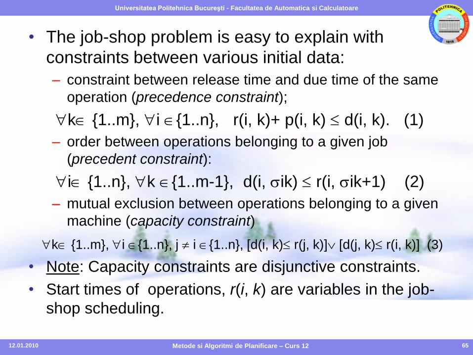
• The job-shop problem is easy to explain with

constraints between various initial data:

– constraint between release time and due time of the same

operation (precedence constraint);

k {1..m}, i {1..n}, r(i, k)+ p(i, k) d(i, k). (1)

– order between operations belonging to a given job

(precedent constraint):

i {1..n}, k {1..m-1}, d(i, ik) r(i, ik+1) (2)

– mutual exclusion between operations belonging to a given

machine (capacity constraint)

k {1..m}, i {1..n}, j i {1..n}, [d(i, k) r(j, k)] [d(j, k) r(i, k)] (3)

• Note: Capacity constraints are disjunctive constraints.

• Start times of operations, r(i, k) are variables in the job-

shop scheduling.



66

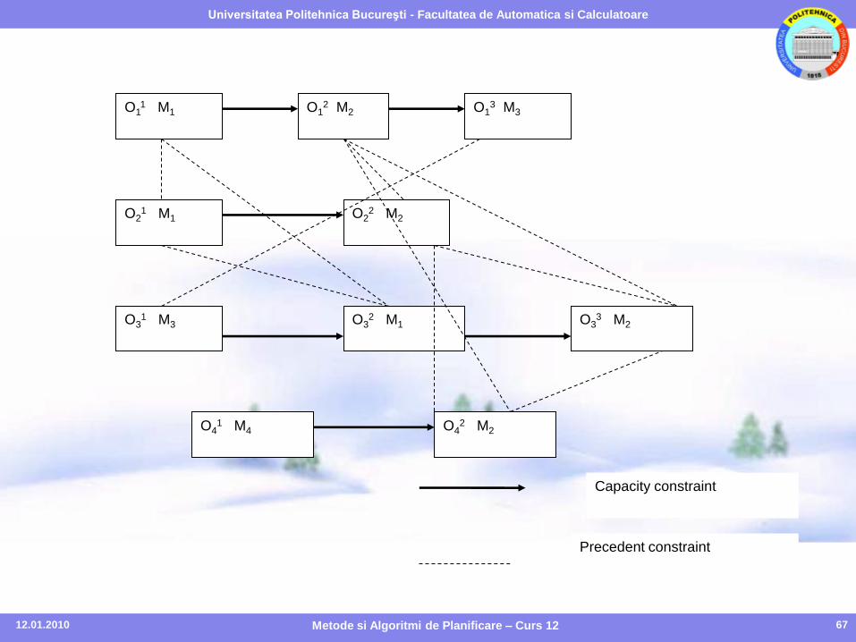
An Instance of Job-Shop Problem

• The following Figure shows a simple job-shop problem with 4 jobs and 4 machines.

• Each node is labeled by the operation that it represents and the machine required by this operation. In this problem 1 = (1,2,3), 2 = (1,2), 3 = (3,1,2), and 4 = (4,2).



67

O11 M1 O1

2 M2 O13 M3

O21 M1 O2

2 M2

O31 M3 O3

2 M1 O33 M2

O41 M4 O4

2 M2

Capacity constraint

Precedent constraint



68

Solving Methods: Method 1

• 1. If all operation have been scheduled then stop, else go to 2.

• 2. Apply the consistency enforcing procedure.

• 3. If a dead-end is detected then backtrack.

• 4. Select the next operation to be scheduled (variable ordering heuristic).

• 5. select a promising assignment for that operation (value ordering heuristic).

• 6. Create a new search state by adding the new assignment to the current partial schedule. Go back to 1.

The following backtracking algorithm can solve the job-shop

scheduling, if combined with some variable ordering and

value ordering.



69

• Consistency enforcing procedure combines 3 types of computations:

– Consistency with respect to precedence constraints. Using an AC-3 algorithm.

– Forward checking with respect to capacity constraints. Enforcing consistency with respect to capacity constraints is more difficult due to the disjunctive nature of these constraints. Whenever a machine is allocated to an operation over some time interval, a “forward checking” mechanism checks the set of remaining possible assignments of other operations requiring that same machine and removes those assignments that would conflict with the new assignment.

– Additional consistency checks with respect to capacity constraints. The consistency enforcing mechanism checks that no two unscheduled operations require overlapping machine/time intervals. This represents a capacity constraint conflict. This additional consistency mechanism has been shown to often increase search efficiency, while only resulting in minor computational overheads.



70

Solving Methods: Method 2 & Method 3

• Method 2.

– Use local search method, such as Tabu Search, Simulated

Annealing.

• Method 3.

– genetic algorithm



Exam’s quizzes

• 1.

• 2.

• 3.


Documents

Metode şi Algoritmi de Planificareandrei.clubcisco.ro/cursuri/5master/g-map/12_AplicatiiMAP.pdfUniversitatea Politehnica Bucureşti - Facultatea de Automatica si Calculatoare Scheduling