Metrics with equatorial singularities on the sphere

HAL Id: hal-00319299https://hal.archives-ouvertes.fr/hal-00319299v7

Submitted on 19 Mar 2013

HAL is a multi-disciplinary open accessarchive for the deposit and dissemination of sci-entific research documents, whether they are pub-lished or not. The documents may come fromteaching and research institutions in France orabroad, or from public or private research centers.

L’archive ouverte pluridisciplinaire HAL, estdestinée au dépôt et à la diffusion de documentsscientifiques de niveau recherche, publiés ou non,émanant des établissements d’enseignement et derecherche français ou étrangers, des laboratoirespublics ou privés.

Metrics with equatorial singularities on the sphereBernard Bonnard, Jean-Baptiste Caillau

To cite this version:Bernard Bonnard, Jean-Baptiste Caillau. Metrics with equatorial singularities on the sphere. Annalidi Matematica Pura ed Applicata, Springer Verlag, 2014, 193 (5), pp.1353-1382. �10.1007/s10231-013-0333-y�. �hal-00319299v7�

https://hal.archives-ouvertes.fr/hal-00319299v7

https://hal.archives-ouvertes.fr

Metrics with equatorial singularities

on the sphere∗

B. Bonnard† J.-B. Caillau‡

September 2012

Abstract

Motivated by optimal control of affine systems stemming from mechanics,metrics on the two-sphere of revolution are considered; these metrics areRiemannian on each open hemisphere whereas one term of the correspon-ding tensor becomes infinite on the equator. Length minimizing curves arecomputed and structure results on the cut and conjugate loci are given,extending those in [11]. These results rely on monotonicity and convexityproperties of the quasi-period of the geodesics; such properties are stud-ied on an example with elliptic transcendency. A suitable deformationof the round sphere allows to reinterpretate the equatorial singularity interms of concentration of curvature and collapsing of the sphere onto atwo-dimensional billiard.

Keywords. two-sphere of revolution, almost and sub-Riemannian me-trics, cut and conjugate locus

MSC classification. 53C17, 49K15

Introduction

In the papers [11, 35] the authors investigate the cut and conjugate loci of aRiemannian metric on the two-sphere of revolution that can be written in thenormal form m(ϕ)dθ2 +dϕ2—where ϕ is the angle along the meridian and θ theangle of revolution—, under the assumption that m(π − ϕ) = m(ϕ) (symmetrywith respect to the equator). Motivated by examples in optimal control, ouraim is to extend these results to metrics of the form

XR(X)dθ2 + dϕ2, X = sin2 ϕ, (1)

∗Supported by ANR Geometric Control Methods (project no. NT09 504490).†Math. Institute, Univ. Bourgogne & CNRS, 9 avenue Savary, F-21078 Dijon

([email protected]). On leave at INRIA, 2004 route des lucioles, F-06902Sophia Antipolis.

‡Same address ([email protected]). Also supported by ConseilRegional de Bourgogne (contract no. 2009-160E-160-CE-160T) and by SADCO Initial Trai-ning Network (FP7 grant no. 264735-SADCO).

1

Metrics with equatorial singularities on the sphere 2

where R is a rational fraction with a single pole at X = 1. The metric isRiemannian on both open hemispheres but has a singularity on the equator.Such metrics arise when one considers the time minimum control of a system

x(t) = u1(t)F1(x(t)) + u2(t)F2(x(t)), u21(t) + u2

2(t) ≤ 1,

with fixed boundary conditions, x(0) = x0, x(tf ) = xf , and it is well knownthat minimizing time amounts to minimizing the length of the curve t 7→ x(t)provided the metric is defined by assuming F1 and F2 orthonormal. For suchproblems, singularities occur when the two vector fields become collinear. Thisleads to the concept of almost-Riemannian metrics [3, 4, 12, 15], and the analysisof such metrics is related to sub-Riemannian geometry [6, 26]. If the distribution{F1, F2} is bracket generating, every pair of points can be joined by a lengthminimizing curve. Moreover, if there exists no abnormal trajectory, each mini-mizing curve is a geodesic, projection on the x-space of the Hamiltonian flowexp t

−→h where

h(z) =12

(H2

1 (z) + H22 (z)

), z = (x, p),

and where Hi(z) = 〈p, Fi(x)〉 are the Hamiltonian lifts of the Fi’s. Denotingexpx0

the exponential mapping

expx0(t, p0) = Π

(exp t

−→h (x0, p0)

)where Π is the projection (x, p) 7→ x, the cut and conjugate loci are defined as inthe Riemannian setting; the cut locus is the set of points where geodesic curvesfail to be minimizing, while the conjugate locus is the image of the critical pointsof the exponential mapping.

In this paper, we generalize to the singular case (1) the results in [11] relatingthe structure of the cut and conjugate loci to the convexity of the quasi-periodof the θ-coordinate: Under appropriate assumptions, the cut locus of a point isreduced to a single segment, and the conjugate locus has at most four cusps.Although similar to the Riemannian case, the singularity of the metric on theequator has two consequences; the injectivity radius is zero and the singularitiesof the conjugate locus of an equatorial point differ. In Section 2, two examplesmotivating this study are presented. One stems from quantum mechanics, theother from space mechanics. Both are limit cases of optimal control problemsnot linear but affine in the control. Section 3 is devoted to the integrabilityproperties of the geodesics of (1), and preliminary computations of the periodand quasi-period of coordinates ϕ and θ are made. The optimality status ofthe geodesics is studied in Section 4 where the main results on the structure ofcut and conjugate loci are established. The second example of §2 is given a fulltreatment in Section 5. In order to be able to apply §4 results, a detailed analysisusing a parameterization of geodesics by elliptic curves is presented. The lastsection accounts for concentration of curvature and collapsing phenomena thatallow to reinterpretate the effect of the equatorial singularity on the metric.


1 Preliminaries

We consider the metric (1) on S2 where (θ, ϕ) are the coordinates induced bythe covering of the sphere minus poles

R× (0, π) 3 (θ, ϕ) 7→ (sinϕ cos θ, sinϕ sin θ, cos ϕ).

The function R is a rational fraction with a single pole of order p at X = 1,

R(X) =p∑

k=0

ak

(1−X)k, a0, . . . , ap−1 ≥ 0, ap > 0 (p ≥ 1). (2)

We assume that the normalization condition a0 + · · · + ap = 1 holds. Themetric is Riemannian on hemispheres with a singularity on the equator whenϕ = π/2 since R(X) →∞ when X → 1. It is a standard fact that Riemanniangeometry can be recast in the Hamiltonian setting of optimal control: On eachopen hemisphere, finding a length minimizing curve connecting two points x0,xf , is equivalent to finding a measurable control function u : [0, tf ] → R2 suchthat almost everywhere

x(t) = u1(t)F1(x(t)) + u2(t)F2(x(t)), u21(t) + u2

2(t) ≤ 1, (3)

x(0) = x0, x(tf ) = xf ,

and such that the final time tf is minimized. In the previous coordinates, thevector fields are (because of the topology of the 2-sphere, one cannot providean orthonormal frame of vector fields globally defined on S2)

F1(θ, ϕ) :=1

sinϕ

√1/R(X)

∂

∂θ, F2(θ, ϕ) :=

∂

∂ϕ(4)

as

Lemma 1. 1/R(X) has a smooth square root.

Proof. One has1

R(X)=

cos2p ϕ

ap + · · ·+ a0 cos2p ϕ

and ap + · · ·+ a0 cos2p ϕ ≥ ap > 0 by virtue of (2).

This optimal control formulation makes sense on the whole sphere: This is how(1) will be understood as a metric defined on all S2 in this paper. Geometrically,the singularity R(1) = ∞ forces length minimizing curves to be vertical (directedalong meridians) when crossing the equator.Remark 1. The singularity here is not a degeneracy of the Riemannian tensoron the tangent space as in, e.g., [30] but a degeneracy of a positive tensor onthe cotangent space.

An appropriate algebraic setting for such a metric is the notion of generalizedsub-Riemannian metrics (see [6, 24]) or almost-Riemannian metrics (see [1, 3, 4,12]). Let g0 be the round metric on the sphere; to (1) is associated the followingmorphism of fibre bundle:1

f : (TS2, g0) → TS2

1That is id-morphism, according to [16] terminology: Base points are unchanged by themorphism, and fibres are linearly sent to fibres.


such that f is the identity on the fibres above the poles and

f(θ,ϕ) :∂

∂θ7→

√1/R(X)

∂

∂θ,

∂

∂ϕ7→ ∂

∂ϕ

otherwise. This morphism induces an application between vector fields on thesphere, f∗ : Γ(TS2) → Γ(TS2); if F ∈ Γ(TS2),

f∗(F )(x) := fx(F (x)), x ∈ S2.

Although the direct image f(TS2) is not a fibre bundle,

∆ := f∗(Γ(TS2)) ⊂ Γ(TS2)

is a well defined submodule over smooth functions. For x ∈ S2 and v ∈ ∆x :={F (x), F ∈ ∆}, define

gx(v) := inf{g0x(u) | fx(u) = v}.

Outside poles,

gx(v) = inf{u21 + u2

2 | u1F1(x) + u2F2(x) = v}.

Then, given two points x0, xf on the sphere, set

d(x0, xf ) := inf∫ tf

0

√gx(t)(x(t)) dt

where the infimum is taken over all Lipschitz trajectories x such that

x(t) ∈ ∆x(t), t ∈ [0, tf ] (a.e.)

x(0) = x0, x(tf ) = xf .

The set of such horizontal trajectories is not empty as is clear from the proof of

Proposition 1. d defines a complete distance on S2 that induces the usualtopology on the sphere.

To prove this fact, one defines recursively the flag associated with ∆ by meansof the Lie bracket of vector fields,

∆1 := ∆, ∆k+1 := ∆k + [∆,∆k]

with [∆,∆k] := {[F,G] | F ∈ ∆, G ∈ ∆k}, k ≥ 1.

Lemma 2. For all x ∈ S2, ∆p+1x = TxS2.

Proof. Outside the equator, F1 and F2 have rank two, so the verification isrestricted to ϕ = π/2 where F1 vanishes. Since R has an order p pole,

(adp F2)F1(θ, ϕ) =dp

dϕp[(1/ sinϕ)

√1/R(X)]︸︷︷︸

6=0 at ϕ=π/2

∂

∂θ

so brackets of length at most p+1 span everywhere the whole tangent space.


Proof of Proposition 1. According to lemma 2, ∆ is bracket generating so thereexist, for any pair of points on the sphere, Lipschitz curves almost everywheretangent to ∆ connecting them by Chow-Rashevsky theorem. On the compactmanifold S2, Filippov theorem [5] then asserts existence of time minimizingcurves among those. That the metric induces the canonical manifold topologyis another consequence of Chow-Rashevsky [24].

Remark 2. As explained in [3], generic (in the sense of Whitney) almost-Rieman-nian metrics on the sphere are such that, for all x ∈ S2, either ∆x (regular point),∆2

x (Grusin point) or ∆3x (tangency point) span the tangent space. According

to Lemma 2, the situation we consider is not generic for p ≥ 3.

2 Motivating examples

The following Hamiltonian on S2 is considered in [9]:

H(θ, ϕ, pθ, pϕ) = −δ cos ϕ sinϕ pϕ +12

(p2

θ

tan2 ϕ+ p2

ϕ

). (5)

It originates in quantum mechanics and partly describes the energy minimumcontrol of a spin 1/2 particle in a magnetic field. When the parameter δis zero, this Hamiltonian corresponds exactly to the metric (1) obtained forR(X) = 1/(1 − X) (geodesics are integral curves of an appropriate quadraticHamiltonian—see the beginning of §3). As explained in §4, a local model nearthe singularity ϕ = π/2 is the so-called Grusin metric on R2 [14, 22]

dx2 +dy2

x2·

For this reason, the metric defined by (5) when δ = 0 is called Grusin metric onthe sphere. In contrast to the analogous metric on the plane, it has peculiarities(e.g., meridional cusps of conjugate loci, see §4) due to the topology of thesphere. Like the second example, it is also connected with space mechanics (see[11]).

Consider a controlled dynamical system of the form

dx

dl(l) =

m∑i=1

ui(l)Fi(l, x(l)) (6)

on a smooth n-dimensional manifold X where the Fi : R ×X → X are vectorfields parameterized by l and periodic, F (l, x) = F (l + 2π, x) for all l ∈ R andx ∈ X. This dynamics is actually a particular case of an (autonomous) affinein the control system, as we may define the vector fields

F0(x) := ω(x)∂

∂l, Fi(x) := ω(x)

n∑j=1

〈dxj , Fi〉∂

∂xj, i = 1, . . . ,m,

with x := (l, x) ∈ X := R×X and write

dx

dt(t) = F0(x(t)) +

m∑i=1

ui(t)Fi(x(t)).


The pulsation ω is any 2π-periodic in l positive function on X relating the twotimes of the system, t and l (the latter being understood as an angular length).The periodic vector fields Fi induce vector fields on S1 ×X and it is appealingto use averaging [27] to define

F i(x) :=12π

∫ 2π

0

Fi(l, x) dl.

We consider instead the Hamiltonian associated with the L2dt-minimization ofthe control,

H(l, x, p) =ω(l, x)

2

m∑i=1

〈p, Fi(l, x)〉2.

Then,

H(x, p) :=12π

∫ 2π

0

H(l, x, p) dl

remains a positive quadratic form in the adjoint variable, p. Under the standardassumption that the Fi, i = 0, . . . ,m, are bracket generating, one expects therank of this quadratic form to be maximum and equal to n. The case being,one can find n independent vector fields F i such that

H(x, p) =12

n∑i=1

〈p, F i(x)〉2.

Singularities of two types may exist though. First, such implicitly defined vectorfields need not be smooth on X, even in the analytic situation.2 In addition,the rank of the form may not be constant on X and drop at some points.This phenomenon accounts for the existence of an equatorial singularity in thefollowing case.

On X = R∗+ ×D, D being the open unit Poincare disk, set

F1 := − 3(1− e2)wn1/3(1 + e cos v)2

∂

∂n+

2(1− e2)2

n4/3(1 + e cos v)2w

[(e + cos v)

∂

∂e+

sin v

e

∂

∂θ

]with

v := l − θ, w :=√

1 + 2e cos(l − θ) + e2 ,

and

ω(l, x) :=n(1 + e cos(l − θ))2

(1− e2)3/2·

Here, x = (n, e, θ) ∈ R∗+×R∗

+×R are coordinates on the positive line times thepointed disk. They are used in space mechanics to represent the geometry ofplane elliptic trajectories in the controlled two-body problem [10]: n is the meanmotion (that is n = a−3/2 where a is the semi-major axis), e is the eccentricity,and θ is the argument of the pericenter. The averaging procedure just describedleads to [10]

H(n, e, θ, pn, pe, pθ) =9n1/3

2p2

n +1

n5/3h(e, θ, pe, pθ)

2See, e.g., §3.2 in Bonnard, B.; Caillau, J.-B.; Picot, G. Geometric and numerical tech-niques in optimal control of two and three-body problems. Commun. Inf. Syst. 10 (2010),no. 4, 239–278.


with

h(e, θ, pe, pθ) =12

[4(1− e2)3/2

1 +√

1− e2p2

e +4(1− e2)

(1 +√

1− e2)p2

θ

e2

].

Proposition 2. H, h and pθ are independent first integrals in involution; inparticular, H is Liouville integrable.

Proof. The Poisson bracket of H and h is

{H, h} =∂H

∂pn

∂h

∂n− ∂H

∂n

∂h

∂pn+

1n5/3

{h, h} = 0,

the rest being obvious.

The integration of H may so be performed by integrating h. This two-di-mensional Hamiltonian (which retains the linear first integral pθ) is lifted fromthe Poincare disk to S2 using the following compactification: In the covering(θ, ϕ) ∈ R× (0, π) of the sphere minus poles where

e = sinϕ√

1 + cos2 ϕ ,

one has

h(θ, ϕ, pθ, pϕ) =12

[4 cos4 ϕ

sin2 ϕ(2− sin2 ϕ)2p2

θ + p2ϕ

].

The rank of this quadratic form in (pθ, pϕ) drops from 2 to 1 when ϕ = π/2.Actually, h is exactly associated to the metric (1) with

R(X) =(

1−X/21−X

)2

=14

[1 +

21−X

+1

(1−X)2

]·

This metric with an order two equatorial singularity will be referred to as the(1, 2, 1) case (according to coefficients involved in the series) and studied inSection 5.

Remark 3. The Hamiltonian (5) in the first example can either be interpre-tated as stemming from an affine controlled system, or as defining a pseudo-Riemannian metric (see [9]). In constrast with the sub-Riemannian case thatis characterized by linearity in the control, time minimization (with a boundedcontrol) and minimization of the L2-norm (with a prescribed final time) of affinesystems cease to be equivalent.

3 Integrability properties

As time minimizing curves of the control system (3), geodesics satisfy Pontrjaginmaximum principle [5, 13]: If x is a shortest time trajectory generated by theoptimal control u : [0, tf ] → R2, there exist a nonpositive constant p0 ≤ 0 and aLipschitzian lift (x, p) : [0, tf ] → T ∗S2 of the trajectory to the cotangent bundlesuch that (p0, p) 6= (0, 0) and

x(t) =∂H

∂p(x(t), p(t), u(t)), p(t) = −∂H

∂x(x(t), p(t), u(t)), t ∈ [0, tf ] (a.e.),


where

H : T ∗S2 ×R2 → R, H(x, p, u) := p0 + u1H1(x, p) + u2H2(x, p).

The Hi : T ∗S2 → R are the Hamiltonian lifts of the two vector fields (4),

Hi(x, p) := 〈p, Fi(x)〉, i = 1, 2.

Besides, the following maximization condition holds,

H(x(t), p(t), u(t)) = max|v|≤1

H(x(t), p(t), v), t ∈ [0, tf ] (a.e.)

As a result, the Hamiltonian evaluated along the extremal (x, p, u) is almosteverywhere equal to a constant; since the final time is free, this constant iszero. The previous relations are homogeneous in (p0, p) and there are two cases:Either p0 = 0 (abnormal case), or p0 < 0 (normal case).

Lemma 3. Abnormal trajectories are stationary equatorial curves.

Proof. Assume p0 = 0. Then H = u1H1 + u2H2 has to be zero and maximizedalong the extremal; necessarily, the two Lipschitz functions H1 and H2 mustvanish identically on [0, tf ] (the maximum would otherwise be positive). As aresult, for any time t, p(t) is orthogonal to the span at x(t) of F1 and F2. Ifthere exists t ∈ [0, tf ] such that ϕ(t) 6= π/2, the span at such an x(t) is the wholetangent space, so p(t) = 0. As p is solution of the linear differential equation

p(t) = −∂H

∂x(x(t), p(t), u(t)) = −p(t) [F ′

1(x(t)) + F ′2(x(t))] ,

p is identically zero, which contradicts (p0, p) 6= (0, 0). So ϕ ≡ π/2; then

θ(t) = u1(t)√

1/R(X) |X=1 = 0

so θ is also constant.

We disregard theses trivial curves and normalize p0 to −1.

Scholium. Geodesics of (1) are integral curves of the quadratic Hamiltonian

h(θ, ϕ, pθ, pϕ) :=12

(p2

θ

XR(X)+ p2

ϕ

)(7)

restricted to the level set {h = 1/2}.

Proof. Let u be a minimum time control, and let (x, p, u) be the associatedextremal. The normal Hamiltonian −1+u1H1+u2H2 is zero along the extremal,so (H1,H2) does not vanish. Because of the maximization condition,

u(t) =(H1,H2)√H2

1 + H22

(x(t), p(t)) a.e.

Then,

x(t) = u1(t)F1(x(t)) + u2(t)F2(x(t)) (8)= H1(x(t), p(t))F1(x(t)) + H2(x(t), p(t))F2(x(t))


since H21 + H2

2 = 1 on {H = 0} (that is {h = 1/2}), so

x(t) =∂h

∂p(x(t), p(t)) a.e.

One similarly verifies that

p(t) = −∂h

∂x(x(t), p(t)) a.e.

Remark 4. Such geodesics are arc length parameterized as (8) implies that

gx(t)(x(t)) = u21(t) + u2

2(t) = 1 a.e.

As θ is a cyclic variable (symmetry of revolution—see [7] for a general reference)of h, pθ is a linear first integral and

Proposition 3. h is Liouville integrable. The coordinate ϕ is parameterized bya hyperelliptic curve of genus at most p.

Proof. X = sin2 ϕ, so X2 = 4X(1−X)ϕ2. On {h = 1/2},

X2 = 4X(1−X)(

1− p2θ

XR(X)

),

so

Y 2 = 4(1−X)(ap + · · ·+a0(1−X)p)[X(ap + · · ·+a0(1−X)p)−p2θ(1−X)p] (9)

with Y = (ap + · · · + a0(1 −X)p)X. The right hand side of (9) has degree atmost 2(p + 1), so the genus of the complex curve is at most p.

SetΓ(ϕ) :=

1XR(X)

, ϕ ∈ (0, π).

Consider the extremal departing from ϕ0 6= 0 (π) (not a pole), θ0 being normal-ized to 0 and defined by a positive pθ (the degenerate case pθ = 0 correspondingto meridians—which are the only extremals passing through the poles) and non-negative pϕ0 =

√1− Γ(ϕ0)p2

θ. Along the extremal, ϕ first vanishes when ϕ isequal to ϕ1 := π − Γ−1(p−2

θ ) since

Lemma 4. Γ is a strictly decreasing one-to-one mapping between (0, π/2] andR+ such that Γ(π − ϕ) = Γ(ϕ).

Proof. One hasdΓdX

= −R(X) + XR′(X)(XR(X))2

with

R′(X) =p∑

k=1

kak

(1−X)k+1·

Since dX/dϕ = 2 sin ϕ cos ϕ is positive on (0, π/2), the conclusion follows.


As Γ′ does not vanish on (0, π/2),

1− Γ(ϕ)p2θ = O(ϕ1 − ϕ)

in the neighbourhood of π−Γ−1(p−2θ ), and the following integral (depending on

pθ and ϕ0) is well-defined,

t1 :=∫ π−Γ−1(p−2

θ )

ϕ0

dϕ√1− Γ(ϕ)p2

θ

·

Lemma 5. The axial symmetry σ1 with respect to θ(t1) is an inner symmetryof the extremal.

Proof. Set

θ(t) := 2θ(t1)− θ(2t1 − t), pθ(t) := pθ(t),ϕ(t) := ϕ(2t1 − t), pϕ(t) := −pϕ(2t1 − t),

and check that new curve is still an extremal, passing through the same pointof the cotangent bundle at t1 since pϕ(t1) = 0.

Necessarily, π − Γ−1(p−2θ ) ≥ π − ϕ0, so there also exists t′1 ≤ t1 such that

ϕ(t′1) = π − ϕ0. Using the previous axial symmetry, we deduce the existence oft2 := 2t1 − t′1 ≥ t1 such that, again, ϕ(t2) = π − ϕ0. Using now the equatorialsymmetry of Γ,

Γ(π − ϕ) = Γ(ϕ),

the following is clear.

Lemma 6. The central symmetry s2 with respect to (θ(t2)/2, π/2) defines an-other extremal with the same initial condition.

Proof. Set

θ(t) := θ(t2)− θ(t2 − t), pθ(t) := pθ(t),ϕ(t) := π − ϕ(t2 − t), pϕ(t) := pϕ(t2 − t).

The new curve is still an extremal since

˙θ(t) = Γ(π − ϕ(t))pθ = Γ(ϕ(t))pθ, ˙pϕ(t) =

12Γ′(π − ϕ(t))p2

θ = −12Γ′(ϕ(t))p2

θ,

and θ0 = 0 = θ0, ϕ0 = π − (π − ϕ0) = ϕ0.

Finally denote t3 the point such that ϕ(t3) = π/2 ≤ π−ϕ0, and remark that thecentral symmetry σ2 with respect to (θ(t3), π/2) leaves the extremal invariant.Since the axial symmetry s1 with respect to θ = 0 obviously defines anotherextremal originating from the same point, we conclude that the group generatedby s1 and s2 acts on the set of extremals with same initial condition, while thegroup generated by σ1 and σ2 defines inner symmetries of each extremal. Thecomposition rules indicate in both cases that the underlying group is the four-order abelian Klein group,

V = Z/2Z× Z/2Z ' {id, s1, s2, s1s2} ' {id, σ1, σ2, σ1σ2}.


Proposition 4. Given any initial condition, the Klein group acts on the setof extremals issuing from the point. It also defines inner symmetries of anyextremal.

An extremal is said to be a pseudo-equator whenever ϕ(0) = pϕ(0) is equal tozero, whereas the equator itself cannot be an extremal because of the singularity.

Lemma 7. Every extremal that is not a meridian is a pseudo-equator.

Proof. For pθ positive and pϕ0 nonnegative (the other cases are deduced by sym-metry), there exists ϕ0 = Γ−1(p−2

θ ) such that, up to a time shift, the extremalis the pseudo-equator with initial condition ϕ0.

Conversely, any pseudo-equator meets ϕ = π/2 as one understands from theanalysis of symmetries. Taking ϕ0 = π/2 as new initial condition and retainingthe same value for pθ provides the same geodesic, up again to a time shift. Asa result, rather than parameterizing extremals using both ϕ0—we set θ0 = 0thanks to the symmetry of revolution—and pθ, one may either parameterize byϕ0 ∈ (0, π/2) alone using the fact all geodesics (with the exception of meridians,pθ = 0) are pseudo-equators (then, implicitly, p2

θ = 1/Γ(ϕ0), ϕ0 6= π/2 since theequator is not a geodesic), or parameterize by their Clairaut constant pθ ∈ R∗

+,considering only the initial condition at singularity, ϕ0 = π/2. The second pointof view reduces the study of geodesics to those starting at singularity.

Proposition 5. On every extremal, the coordinate ϕ is periodic with period

T (pθ) = 4∫ π/2

Γ−1(p−2θ )

dϕ√1− Γ(ϕ)p2

θ

,

and θ(t + T ) = θ(t)±∆θ (sign depending on the sign of pθ) with quasi-period

∆θ(pθ) = 4∫ π/2

Γ−1(p−2θ )

Γ(ϕ)pθdϕ√1− Γ(ϕ)p2

θ

·

Proof. According to the previous analysis, it is enough to check the result onpseudo-equators. But then, t1 = t2 = t3 = 2t4, so setting T := 2t1 and usingthe axial symmetry with respect to θ(t1) gives the result since ϕ(T ) = ϕ(0),pϕ(T ) = −pϕ(0) = 0 = pϕ(0). So θ = Γ(ϕ)pθ is also periodic, which concludesthe proof.

As functions of ϕ0,

T (ϕ0) = 4∫ π/2

ϕ0

dϕ√1− Γ(ϕ)/Γ(ϕ0)

, (10)

and

∆θ(ϕ0) = 4∫ π/2

ϕ0

Γ(ϕ)dϕ√Γ(ϕ0)− Γ(ϕ)

· (11)

These relations actually cover the case of meridians pθ = 0 (i.e. ϕ0 = 0) forwhich T = 2π and ∆θ = 2π (two instantaneous rotations of angle π whencrossing poles at t = π and t = 2π). We end the section with the followingresult that will be used for §5 computations.


Proposition 6. T ′ = pθ∆θ′.

Proof. Write as in [11]

T (pθ) = pθ∆θ(pθ) + 4∫ π/2

Γ−1(p−2θ )

√1− Γ(ϕ)p2

θ dϕ,

so

T ′(pθ) = ∆θ(pθ) + pθ∆θ′(pθ) + 4∫ π/2

Γ−1(p−2θ )

∂

∂pθ

(√1− Γ(ϕ)p2

θ

)dϕ

−8(Γ−1)′(p−2θ )pθ

√1− Γ(ϕ)p2

θ |ϕ=Γ−1(p−2θ )︸︷︷︸

0

= pθ∆θ′(pθ).

4 Cut and conjugate loci

The cut time along a geodesic x, that is along an extremal of the minimum timeproblem (3), is the supremum of times t such that the curve restricted to [0, t]is a shortest time trajectory between x(0) and x(tf ):

tcut := sup{t ≥ 0 | x is minimizing on [0, t]}.

When tcut < ∞, x(tcut) is called a cut point. The set of all cut points ongeodesics departing from a given intial point x0 is the cut locus of x0. A sepa-rating point along the geodesic is a point x(tM ), tM > 0, such that there existsa different geodesic, y, reaching the point at the same time: x(tM ) = y(tM ).The exponential mapping of a fixed point x0 ∈ S2 is

expx0: R∗

+ × T ∗x0

S2 ∩ {h = 1/2} → S2 (12)

(t, p0) 7→ x(t, x0, p0) := Π ◦ exp t−→h (x0, p0)

where Π : T ∗S2 → S2 is the canonical projection and exp t−→h the one-parameter

global subgroup generated by the symplectic gradient of the quadratic Hamil-tonian (7),

−→h (x, p) =

∂h

∂p(x, p)

∂

∂x− ∂h

∂x(x, p)

∂

∂p·

The intersection of the fibre T ∗x0

S2 with {h = 1/2} is a compact oval diffeo-morphic to S1 outside the equator, or the union two lines {pϕ0 = ±1} for anequatorial point. That the subgroup is globally defined in the second case comesfrom the analysis of Section 3: For any pθ ∈ R and pϕ0 = ±1, the coordinates ϕand θ are periodic or quasi-periodic, respectively. A conjugate point along thegeodesic x is a critical value of expx(0); if (tc, p0) is the corresponding criticalpoint, tc is the conjugate time. When tc > 0 is the first conjugate time alongthe geodesic, x(tc) is called a first conjugate point. The set of first conjugatepoints on geodesics departing from x0 is the conjugate locus of x0. Results of


optimal control ensure that local optimality is lost after conjugate points [33].Besides, extremals of such problems have to be smooth so that broken curvesthat are concatenations of minimizing geodesics cannot be minimizing, entailingthat optimality cannot be preserved after separating points, such as those gen-erated by the symmetries between extremals described in the previous section.Separating and conjugate times are so upper bounds of cut times. The followingstandard result remains valid in our setting with singularities.

Proposition 7. Cut points of the metric (1) are either conjugate or separatingpoints.

Lemma 8. Both T and ∆θ vanish when |pθ| → ∞.

Proof. Directly follows from estimates of integrals (10-11) using the fact that Γdoes not vanish identically at ϕ = π/2.

Proof of Proposition 7. Let γ(tcut) be the cut point along the geodesic γ startingfrom x0 = (θ0, ϕ0) and generated by the adjoint vector p0. If the cut point isnot a conjugate point, the exponential mapping is a diffeomorphism in a smallenough neighbourhood V0 of (tcut, p0). Since the metric is complete, there areminimizing extremals γn joining x0 to γn(tn) = γ(tcut + 1/n), tn < tcut + 1/n,for n ≥ 1. First assume that ϕ0 6= π/2. Then the oval h−1(θ0, ϕ0, ·)({1/2}) iscompact, and one can extract a converging subsequence of the (p0n)n generatingthe extremals γn, and thus conclude classically (see, e.g., [32]): p0n → p0 andγn(tn) → γ(tcut); assuming by contradiction that the point is not a separatingone, that is assuming that p0 = p0, implies that for n large enough γn(tn)belongs to expx0

(V0), so that tn = tcut + 1/n, whence the contradiction. Letnow ϕ0 = π/2. Though h−1(θ0, ϕ0, ·)({1/2}) = {pϕ0 = ±1} is not compactanymore, the associated sequence (pθn)n still has to be bounded otherwise therewould exist a subsequence such that |pθn| → ∞. Assume by contradiction thatthis is the case. Because of the central symmetry s2, (∆θ(pθn)/2, π/2) is aseparating point on γn = (θn, ϕn), so tn < T (pθn)/2 and θn(tn) < ∆θ(pθn)/2;as |ϕn| = |pϕn| ≤ 1, |ϕn(tn)− π/2| ≤ T (pθn)/2 and (θn(tn), ϕn(tn)) → (0, π/2)according to Lemma 8. Since γ(tcut + 1/n) = γn(tn), this implies γ(tcut) = x0,which is contradictory. The sequence (pθn)n is hence bounded, and we canconclude as previously.

Cut loci for an analytical Riemannian metric on the sphere are known to be finitetrees whose extremities are conjugate points after the work of Poincare [28, 29,31]. In our case, cut loci have peculiarities due to the symmetry of revolutionand the equatorial singularity (see also Corollary 3 in §6; more generally onsurface of revolutions, see [34]).

Theorem 1. Under the assumption that ∆θ is strictly decreasing for pθ > 0,cut loci of the metric (1) are antipodal subarcs. The cut locus of a pole is reducedto the opposite pole, is equal to the equator minus the point for an equatorialpoint, and to a proper closed subarc of the antipodal parallel otherwise.

Proof. The case of poles is obvious and does not depend on any assumptionon ∆θ since the only extremals through them are meridians. Consider now thesituation ϕ0 = π/2, and show that the exponential mapping is injective on thequadrant ⋃

pθ>0

(0, T (pθ)/2]× {(pθ, 1)},


that is show that subarcs of extremals defined by t ∈ [0, T (pθ)/2], positive pθ andpϕ = +1 do not intersect. If p′θ > pθ, the arc associated with p′θ is strictly belowthe one associated with pθ. Indeed, note that on the first half of such an arct ∈ [0, T (pθ)/4) and ϕ does not vanish so that the curve can be parameterizedby ϕ instead of time. There,

f(ϕ, pθ) :=dθ

dϕ=

Γ(ϕ)pθ√1− Γ(ϕ)p2

θ

is an increasing function of pθ since

∂f

∂pθ(ϕ, pθ) =

Γ(ϕ)(1− Γ(ϕ)p2

θ)3/2> 0.

As geodesics starting from ϕ0 = π/2 cross again the equator at ∆θ(pθ)/2,the assumption ensures that the aforementioned subarcs do not intersect. Weconclude by remarking that the full set of extremals is obtained by consideringthe action of the Klein group on geodesics with same initial condition (see §3).First, the central symmetry s2 that generates intersections at t = T (pθ)/2, thenthe axial symmetry s1 with respect to θ = 0 that generates intersections atθ = π, thus not prior to the previous ones since θ(T (pθ)/2) = ∆θ(pθ)/2, andsince ∆θ(pθ) < 2π for pθ > 0 (by assumption, ∆θ is decreasing, and equalto 2π on meridians, i.e. when pθ = 0). So extremals are optimal up to t =T (pθ)/2, and the corresponding point is a separating point. Since the metricis complete, each point of the equator is reached by such an extremal and theset of separating points, hence the cut locus, is the equator minus the initialpoint itself. Consider finally the case when the initial point is neither polar norequatorial. Then p2

θ belongs to (0, 1/Γ(ϕ0)), and extremals are again optimalup to t = T (pθ)/2. Indeed, there would otherwise exist shorter extremals,which would lead to the existence of shorter extremals for the initial conditionϕ0 = π/2 too, contradicting the previous fact. The central symmetry s2 stillgenerates an intersection at t = T (pθ)/2, and ϕ(T (pθ)/2) = π − ϕ0 so thecorresponding separating point belongs to the antipodal parallel of the startingpoint. Since ∆θ is decreasing, the extremities of the cut are obtained letting pθ

tend to ±(Γ(ϕ0))−1/2 (now finite, since ϕ0 6= π/2), and the subarc is closed.

To study the conjugate loci, we start with some properties of the local modelat singularity. Setting x := π/2 − ϕ and y := θ, since 1 − sin2 ϕ ∼ (π/2 − ϕ)2

when ϕ tends to π/2, a local model for the metric (1) is

ds2 = dx2 +dy2

x2p(13)

where p is the order of the pole. The equatorial symmetry of Γ translatesinto (−x)2p = x2p, so the discrete symmetry group is preserved. Such almost-Riemannian metrics are related to sub-Riemannian distributions. For p = 1,the local model is the Grusin metric ds2 = dx2 + dy2/x2, which is actuallyobtained by projecting the Heisenberg sub-Riemannian distribution [13]. Thisdistribution is indeed defined, up to a renormalization, by the following twovector fields on R3,

F1(x, y, z) :=∂

∂x− y

∂

∂z, F2(x, y, z) :=

∂

∂x+ x

∂

∂z,


and the corresponding sub-Riemannian Hamiltonian is

H(x, y, z, px, py, pz) :=12

[(p2

x + p2y) + 2pz(xpy − ypx) + (x2 + y2)p2

z

],

which suggests to use cylindrical coordinates. In these variables

H(r, θ, z, pr, pθ, pz) =12

[p2

r + (pθ/r + rpz)2].

As θ and z are cyclic, the system is integrable in dimension three, and projectsonto a Hamiltonian in the (r, z)-space with the desired singularity,

h(r, z, pr, pz) :=12(p2

r + r2p2z),

when restricting to pθ = 0. For p = 2, the local model is ds2 = dx2 + dy2/x4,which is connected to the flat Martinet sub-Riemannian distribution. Considerindeed the two vector fields on R3 (see [2])

F1(x, y, z) :=∂

∂x+ y2 ∂

∂z, F2(x, y, z) :=

∂

∂y,

so the sub-Riemannian Hamiltonian is

H(x, y, z, px, py, pz) :=12

[p2

y + (px + y2pz)2].

The two coordinates x and z are cyclic, and the Hamiltonian projects ontoh(y, z, py, pz) := (1/2)(p2

y + y4p2z) in the (y, z)-space when restricting to px = 0,

providing the higher order singularity. Going back to the general case, wecompute geodesics issuing from the origin on the level set {h = 1/2} of theHamiltonian

h(x, y, px, py) :=12(p2

x + x2pp2y)

so that the initial adjoint state belongs to the union of the two lines, {px = ±1}.We set λ := py and restrict to positive λ by symmetry (the trivial geodesics(±t, 0) being obtained for λ = 0). The coordinate x is then

x(t) =1

p√

λq(t p

√λ) , (14)

where q is the solution of

q′2 + q2p = 1, q(0) = 0, q′(0) = 1. (15)

Equivalently,

q−1(u) =∫ u

0

dvp√

1− v2p, u ∈ [−1, 1].

For p = 1, q is harmonic, elliptic for p = 2, hyperelliptic and reciprocal to ahypergeometric function in general. More precisely,

q−1(u) = 2F1(1/2, 1/(2p); 1 + 1/(2p);u2p) · u (16)


where 2F1(a, b; c; z) is the hypergeometric series

2F1(a, b; c; z) =∑n≥0

αnzn

n!,

andα0 := 1,

αn+1/αn := (n + a)(n + b)/(n + c).

The reciprocal of q is hence equal to

q−1(u) =∑n≥0

αnu2np+1

n!

with αn = (a)n(b)n/(c)n for a = 1/2, b = 1/(2p) and c = 1 + 1/(2p), thenotation (a)n standing for the Pochhammer symbol

(a)n := a(a + 1) · · · (a + n− 1).

Here,

α0 = 1, α1 =12· 12p + 1

, α2 =34· 2p + 18p2 + 6p + 1

· · ·

which gives the usual Taylor series of the reciprocal of the sine function forp = 1, arcsinu = u + u3/6 + 3u5/40 + 5u7/112... Eventually, y = λx2p, so

y(t) =1

( p√

λ)p+1r(t p

√λ), (17)

where r is defined by a second quadrature,

r(s) :=∫ s

0

q2p.

Lemma 9.r =

1p + 1

(s− qq′).

Proof. Differentiating and using (15),

1p + 1

(s− qq′)′ =1

p + 1(1− q′2 − qq′′)

= q2p,

hence the result since r(0) = 0.

For any p ≥ 1, symmetry reasons imply that non-trivial minimizing geodesicsemanating from the origin first intersect on the y-axis (see, e.g., Fig. 1). As aconsequence, the cut locus at the origin of the local model is the axis minus theorigin itself (compare with the metric on the sphere, Theorem 1). The conjugatelocus of the origin is obtained from the set of critical values of the exponentialmapping

exp(0,0)(t, λ) = (x(t, λ), y(t, λ)), (t, λ) ∈ (R∗+)2.

Let t1c(λ) denote the first conjugate time along the geodesic defined by λ > 0.


−6 −4 −2 0 2 4 6−15

−10

−5

0

5

10

15

x

y

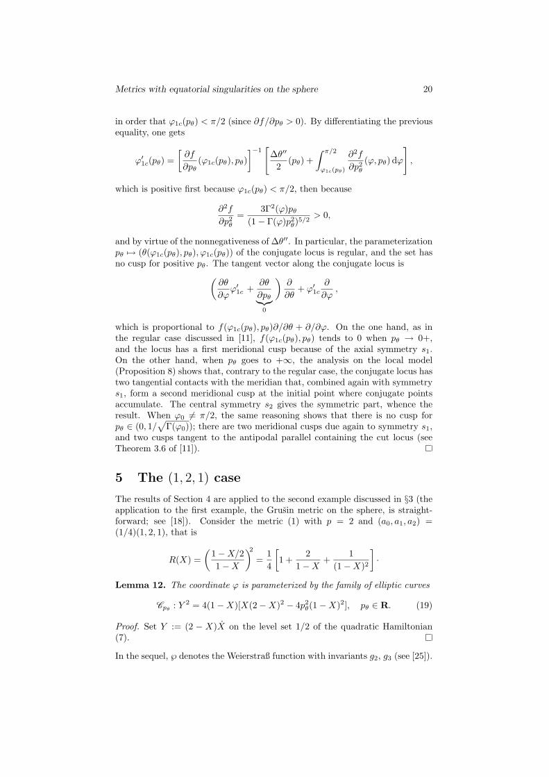
Figure 1: Grusin metric, dx2 +dy2/x2 (p = 1); sphere, wavefront and conjugatelocus of the origin. The wavefront (in blue) is the image of the exponentialmapping for a fixed time, t; it is made of endpoints at time t of geodesics. Thesubset obtained by ruling out the part after the two first self-intersection pointsof the wavefront on the y-axis is the sphere; it is made of points at distance(minimum time) t of the origin. The conjugate locus (in red) is partly drawn(here, it is the set y = ±C1x

2 minus the origin); it is made of critical values ofthe exponential (it contains so the first singularity of the wavefront portrayed).Compare with the Heisenberg metric in [21].

Lemma 10. t1c(λ) = sp/p√

λ where sp is the first positive root of the envelopeequation q = sq′.

Proof. Using (14) and (17), a pair (t, λ) is a critical point of the exponential ifand only if t p

√λ is a solution to

qr′ − (p + 1)q′r = 0.

Expressing r according to Lemma 9, one gets the result.

Proposition 8. The conjugate locus at the origin of ds2 = dx2 + dy2/x2p isthe set y = ±Cpx

p+1 minus the origin where

Cp ∼2√

2p

, p →∞.


Proof. According to Lemma 10,

x(t1c(λ)) =1

p√

λq(sp), y(t1c(λ)) =

1( p√

λ)p+1r(sp),

so points in the conjugate locus lie on the curve y = ±Cpxp+1 where Cp =

r(sp)/qp+1(sp). The whole curve minus (0, 0) is obtained because of symmetries,and conjugate points accumulate towards the origin when |λ| → ∞. It is clearfrom (15) that, as p →∞, q pointwisely converges towards the Lipschitz functionequal to s 7→ s on [0, 1], s 7→ 2 − s on [1, 3]. In particular, the solution sp tothe envelope equation is such that sp → 3−; so q′(sp) → −1/3, q2p(sp) =1− q′2(sp) → 8/9, and qp−1(sp) → 2

√2/3. Now, by virtue of Lemmas 9 and 10,

Cp =1

p + 1sp − q(sp)q′(sp)

qp+1(sp)=

sp

p + 1qp−1(sp) ∼

2√

2p

, p →∞.

Remark 5. For p = 1, q(s) = sin s, r(s) = (1/2)(s − sin t cos t); t1c(λ) = s1/λwhere s1 is the first positive root of

sin s = s cos s.

For p = 2, one obtains

q(s) =√

22

sndn

(s√

2), r(s) =13

[s +

√2

2cn sndn3 (s

√2)

],

in terms of Jacobi functions of modulus k =√

2/2; t1c(λ) = s2/√

λ whereτ = s2

√2 (with s2 < 3) is the first root solution of

sn τ dn τ = τ cn τ.

(Compare with the flat Martinet case in [2].)

Before stating the structure result on the conjugate locus, we finally recallthe following.

Scholium. Along a Jacobi field tangent to the level set of a Hamiltonian qua-dratic in the momentum, the Liouville form is constant.

Proof. In coordinates z = (x, p) ∈ R2n, let H(x, p) = (1/2)(A(x)p|p) with A(x)symmetric; let γ(t) = (z(t), δz(t)) be a Jacobi field, that is z(t) =

−→H (z(t)) and

δz(t) =−→H ′(z(t))δz(t).

Along γ, the time derivative of the Liouville form p dx is

ddt

(p|δx) = (p|δx) + (p|δx)

= −(∇xH|δx) + (p|∇2xpH δx)︸︷︷︸

2(∇xH|δx)

+(p|∇2ppH δp)︸︷︷︸

(∇pH|δp)

= (∇xH|δx) + (∇pH|δp).


Let now z0(σ) be a local parameterization of the level set {H = c}; for aHamiltonian curve z(t, z0(σ)) with initial condition z0(σ), H(z(t, z0(σ))) = c,so

H ′(z(t, z0(σ)))∂z

∂z0(t, z0(σ))z′0(σ)︸︷︷︸

=:δz(t)

= 0.

Along the curve (z(t, σ), δz(t)), the Liouville form is hence constant.

Here, the level set {h = 1/2} of the quadratic Hamiltonian (7) on S2 is locallyparameterized by pθ and the exponential (12) writes

expϕ0(t, pθ) = (θ(t, pθ), ϕ(t, pθ)),

sopθ

∂θ

∂pθ(t, pθ) + pϕ(t, pθ)

∂ϕ

∂pθ(t, pθ) = 0 (18)

since ∂θ(0, pθ)/∂pθ = ∂ϕ(0, pθ)/∂pθ = 0.

Lemma 11. Critical points (t, pθ) of the exponential are characterized eitherby ∂θ(t, pθ)/∂pθ = 0 when ϕ 6= 0, or by ∂ϕ(t, pθ)/∂pθ = 0 when pθ 6= 0.

Proof. The point (t, pθ) is critical if and only if

θ(t, pθ)∂ϕ

∂pθ(t, pθ)− ϕ(t, pθ)

∂θ

∂pθ(t, pθ) = 0.

When pϕ(t, pθ) = ϕ(t, pθ) 6= 0, one can multiply both sides by pϕ and use (18)to get

∂θ

∂pθ(t, pθ)

(pθ θ(t, pθ) + pϕ(t, pθ)ϕ(t, pθ)

)︸︷︷︸

=h=1/2

= 0

whence the result. Similar computation when pθ 6= 0.

Theorem 2. Under the assumption that ∆θ is strictly decreasing and convexfor pθ > 0, conjugate loci of the metric (1) are reduced to the opposite pole forpoles, have four cusps otherwise.

Proof. Let ϕ0 = π/2. Consider an extremal defined by a positive pθ and pϕ0 =+1. For t in (T (pθ)/4, 3T (pθ)/4), ϕ 6= 0 and the extremal can be parameterizedby ϕ according to

θ(ϕ, pθ) =∆θ(pθ)

2+

∫ π/2

ϕ

f(φ, pθ) dφ,

where, as before,

f(ϕ, pθ) =dθ

dϕ=

Γ(ϕ)pθ√1− Γ(ϕ)p2

θ

·

The conjugacy condition is ∂θ/∂pθ = 0 (Lemma 11) so the coordinate ϕ1c(pθ)of the first conjugate point is solution of∫ π/2

ϕ1c(pθ)

∂f

∂pθ(ϕ, pθ) dϕ = −∆θ′(pθ)

2> 0,


in order that ϕ1c(pθ) < π/2 (since ∂f/∂pθ > 0). By differentiating the previousequality, one gets

ϕ′1c(pθ) =[

∂f

∂pθ(ϕ1c(pθ), pθ)

]−1[

∆θ′′

2(pθ) +

∫ π/2

ϕ1c(pθ)

∂2f

∂p2θ

(ϕ, pθ) dϕ

],

which is positive first because ϕ1c(pθ) < π/2, then because

∂2f

∂p2θ

=3Γ2(ϕ)pθ

(1− Γ(ϕ)p2θ)5/2

> 0,

and by virtue of the nonnegativeness of ∆θ′′. In particular, the parameterizationpθ 7→ (θ(ϕ1c(pθ), pθ), ϕ1c(pθ)) of the conjugate locus is regular, and the set hasno cusp for positive pθ. The tangent vector along the conjugate locus is(

∂θ

∂ϕϕ′1c +

∂θ

∂pθ︸︷︷︸0

)∂

∂θ+ ϕ′1c

∂

∂ϕ,

which is proportional to f(ϕ1c(pθ), pθ)∂/∂θ + ∂/∂ϕ. On the one hand, as inthe regular case discussed in [11], f(ϕ1c(pθ), pθ) tends to 0 when pθ → 0+,and the locus has a first meridional cusp because of the axial symmetry s1.On the other hand, when pθ goes to +∞, the analysis on the local model(Proposition 8) shows that, contrary to the regular case, the conjugate locus hastwo tangential contacts with the meridian that, combined again with symmetrys1, form a second meridional cusp at the initial point where conjugate pointsaccumulate. The central symmetry s2 gives the symmetric part, whence theresult. When ϕ0 6= π/2, the same reasoning shows that there is no cusp forpθ ∈ (0, 1/

√Γ(ϕ0)); there are two meridional cusps due again to symmetry s1,

and two cusps tangent to the antipodal parallel containing the cut locus (seeTheorem 3.6 of [11]).

5 The (1, 2, 1) case

The results of Section 4 are applied to the second example discussed in §3 (theapplication to the first example, the Grusin metric on the sphere, is straight-forward; see [18]). Consider the metric (1) with p = 2 and (a0, a1, a2) =(1/4)(1, 2, 1), that is

R(X) =(

1−X/21−X

)2

=14

[1 +

21−X

+1

(1−X)2

]·

Lemma 12. The coordinate ϕ is parameterized by the family of elliptic curves

Cpθ: Y 2 = 4(1−X)[X(2−X)2 − 4p2

θ(1−X)2], pθ ∈ R. (19)

Proof. Set Y := (2 − X)X on the level set 1/2 of the quadratic Hamiltonian(7).

In the sequel, ℘ denotes the Weierstraß function with invariants g2, g3 (see [25]).


Proposition 9.

sin2 ϕ =℘(z)− 4/3℘(z)− 1/3

, z ∈ R,

t = z +1

℘′(a)

[2ζ(a)z + ln

σ(z − a)σ(z + a)

]z

0

with a such that ℘(a) = 1/3 and invariants

g2 =163

+ 16p2θ, g3 =

6427

− 163

p2θ. (20)

Proof. The rational transform

u =13

+1

1−X, v = u2Y,

sends to infinity the fixed root X = 1 in the right hand side of (19), and allowsto recast the equation of Cpθ

under the canonical form v2 = 4u3− g2u− g3 withinvariants (20). When parameterizing the elliptic curve Cpθ

by the Weierstraßfunction, (u, v) = (℘(z), ℘′(z)), only the unbounded component of the real cubichas to be used since X = sin2 ϕ ∈ (0, 1] (that is ℘(z) > 4/3), so z ∈ R. In thisparameterization, the change of time from z to t verifies

dt

dz= 1 +

1℘(z)− 1/3

> 0. (21)

Introducing Weierstraß functions ζ and σ (℘ = −ζ ′ and ζ = σ′/σ), one has (see[23]) ∫

℘′(a) dz

℘(z)− ℘(a)= 2ζ(a)z + ln

σ(z − a)σ(z + a)

·

For a geodesic originating from the singularity, ϕ = π/2 at t = 0 which corres-ponds to z = 0.

As a function of z, the coordinate ϕ is a doubly periodic meromorphic function.Its lattice of periods 2ωZ+ 2ω′Z depends on pθ (the Weierstraß half-periods ω,ω′ are functions of pθ) and is real rectangular: ω ∈ R, ω′ ∈ iR, and the periodscan be choosen so that their ratio τ := ω′/ω belongs to the Poincare upperhalf-plane H = {x + iy ∈ C, y > 0}. Lattices are classified up to conformaltransformations; these transformations are Mobius transforms in the Fuschianmodular subgroup PSL(2,Z) = SL(2,Z)/ ± id of automorphisms of H, so themoduli space of congruences of lattices is H/PSL(2,Z). The modular function jestablishes a one-to-one correspondence between these moduli and the complexplane; in terms of the invariants of the elliptic curve,

j(τ) =g32

∆

where ∆ = g32−27g2

3 is the discriminant of the elliptic curve with ratio of periodsτ . For the family of elliptic curves Cpθ

(see (20)),

j(τ(pθ)) =16(1 + 3p2

θ)3

27p2θ(8 + 13p2

θ + 16p4θ)· (22)


Corollary 1. The number of conformal classes associated with Cpθis

– equal to 1 for pθ ∈ (0, 1/2) ∪ {2/3},

– equal to 2 for pθ ∈ {1/2,√

2},

– equal to 3 for pθ ∈ (1/2, 2/3) ∪ (2/3,√

2) ∪ (√

2,∞).

The only square lattice is obtained for pθ = 2/3.

Proof. The rational fraction (22) has exactly one global minimum at pθ = 2/3and one local maximum at pθ =

√2. Moreover,

j(τ(pθ)) =2827

− 16(p2θ − 1/4)(p2

θ − 2)2

27p2θ(8 + 13p2

θ + 16p4θ)

showing that the value of the local maximum is also attained when pθ = 1/2.

Proposition 10.T (pθ)

4= (1 + β)ω − bη mod

π

2where η := ζ(ω), b := Im a and β := Im ζ(a).

Lemma 13. For all pθ > 0, (1/3,±2i) belongs to the bounded component of theimaginary cubic Cpθ

.

Proof.

4(1/3)3 − (1/3)g2 − g3 =427

− 13

(163

+ 16p2θ

)−

(6427

− 163

p2θ

)= (±2i)2.

Proof of Proposition 10. As X = sin2 ϕ, the period of X is half the period of ϕso

T (pθ)2

=∫ 2ω

0

dt

dz= 2ω +

1℘′(a)

[2ζ(a)z + ln

σ(z − a)σ(z + a)

]2ω

0

. (23)

According to [23, p. 170],

ln[σ(2ω − a)

σ(−a)σ(a)

σ(2ω + a)

]= ln e−4ηa = −4ηa mod 2iπ.

The term in brackets in (23) has to be positive because of (21), so ℘′(a) = +2iby the previous lemma (℘(a) = 1/3) and

T (pθ)4

= ω +ωζ(a)− ηa

imod

π

2·

The bounded component of the imaginary cubic is parameterized by z ∈ ω + iRso a = ω + ib and ζ(a) = η + iβ for some real b and β.

In order to verify the assumptions of Theorems 1 and 2, one has to differentiatethe quasi-period ∆θ with respect to pθ. By means of Proposition 6, it sufficesto compute derivatives of the period T . Define

∂ :=1δ

ddpθ

, δ :=∆

256pθ= pθ(8 + 13p2

θ + 16p4θ).


Lemma 14.

∂ω = −Aω −Bη, ∂b = −Ab−Bβ + D,∂η = Cω + Aη, ∂β = Cb + Aβ + E,

with A, B, C, D, E in R[pθ],

A =13(4 + 13p2

θ + 24p4θ), B = −2 + p2

θ, C =49(−2− 5p2

θ + 3p4θ),

D = 2 + 6p2θ, E =

13(−4 + 9p2

θ).

Proof. The derivatives of the (half) period and quasi-period ω and η = ζ(ω) of℘ and ζ, respectively, with respect to the invariants g2, g3 are known (see [23,p. 307]), and

∂ =323

(3

∂

∂g2− ∂

∂g3

)according to (20). Moreover,

℘(a) = ℘(a(pθ), pθ) =13

implies ℘′(a)∂a + ∂℘(a) = 0,

so ∂a = − 12i

∂℘(a)

(because ℘′(a) = 2i), and one also knows the derivatives of ℘ (and ζ) withrespect to g2, g3 (see [23, p. 298]). Then ∂b = Im ∂a. Similarly,

∂[ζ(a(pθ), pθ)] = −℘(a)∂a + ∂ζ(a) = −13∂a + ∂ζ(a)

and ∂β is obtained taking the imaginary part.

Lemma 15. ∂T is R[pθ]-linear in (ω, η),

∂T (pθ)4

= −(A + E)ω − (B + D)η.

Proof. Applying Lemma 14 rules to T , which is bilinear in (ω, η, b, β), one ob-serves that the coefficients of b and β cancel.

Proposition 11.

∆θ′(pθ) = − 48 + 13p2

θ + 16p4θ

[23(11 + 12p2

θ)ω + 7η

],

∆θ′′(pθ) =4

pθ(8 + 13p2θ + 16p4

θ)2×[

23(24 + 181p2

θ + 830p4θ + 480p6

θ)ω + (−24 + 143p2θ + 400p4

θ)η]

.

Proof. Lemma 15 combined with Proposition 6 gives the first order derivativeof the quasi-period; the second order one is obtained by applying the previousrules anew.


The penultimate result of the section ensures that the cut and conjugate loci inthe (1, 2, 1) case have the structure described in Theorem 1 and Theorem 2.

Theorem 3. ∆θ′ < 0 ≤ ∆θ′′ in the (1, 2, 1) case.

Proof. The first derivative ∆θ′, expressed as linear combination of the nonneg-ative (quasi-)periods ω and η, is obviously negative. To obtain nonnegativity of∆θ′′, one has to check the sign of

23(24 + 181p2

θ + 830p4θ + 480p6

θ)ω + (−24 + 143p2θ + 400p4

θ)η

= 24(23ω − η) + (

23181ω + 143η)p2

θ + (23830ω + 400η)p4

θ +23480ωp6

θ

= 24(23ω − η + p2

θ) + (23181ω + 143η − 24)p2

θ + (23830ω + 400η)p4

θ +23480ωp6

θ.

Let us denote

pθ1 :=120

√−143 + 7

√1201

2

the positive root of −24 + 143p2θ + 400p4

θ, it is enough to verify that

23ω − η + p2

θ ≥ 0 and23181ω + 143η − 24 ≥ 0

on [0, pθ1]. Now, as pθ tends to 0, η/ω degenerates to (3/2)g3/g2|pθ=0 = 2/3(see [23]), so 2ω/3− η + p2

θ vanishes when pθ → 0. Moreover, (2ω/3− η + p2θ)′

is equal to

1pθ(8 + 13p2

θ + 16p4θ)

[(16− 2

3ω − 5η)p2

θ + (26− 203

ω − 8η)p4θ + 32p6

θ

].

Using the coarse estimates ω ∈ [1, 2] and η ∈ [1/2, 1] on [0, pθ1], one has

16− 23ω − 5η ≥ 25

3and 26− 20

3ω − 8η ≥ 14

3,

so nonnegativity of the derivative and the function (2/3)ω − η + p2θ follows on

this interval. The same holds for (2/3)181ω + 143η − 24 that is bounded belowby 1009/6 on [0, pθ1], whence the result.

The condition for a geodesic to be closed is ∆θ ∈ πQ (rationality of ∆θ/π),so that asymptotics when pθ → ∞ measure the density of closed curves in theneighbourhood of the equator. This is also related to optimality conditionsthrough injectivity radius (see [8] in the Riemannian case). The asymptoticsbelow use quadratures by means of elliptic integrals detailed in the appendix.

Proposition 12. In the neighbourhood of meridians,

T ∼ 2π(1− 3√

28

p2θ +

105√

2512

p4θ), ∆θ ∼ 2π(1− 3

√2

4pθ +

35√

2128

p3θ), pθ → 0.

and in the neighbourhood of the equator,

T ∼ 4(2−√

2)K(3−2√

2)p−1/2θ , ∆θ ∼ 4

3(2−

√2)K(3−2

√2)p−3/2

θ , pθ →∞.


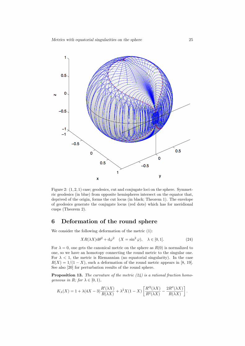
Figure 2: (1, 2, 1) case; geodesics, cut and conjugate loci on the sphere. Symmet-ric geodesics (in blue) from opposite hemispheres intersect on the equator that,deprived of the origin, forms the cut locus (in black; Theorem 1). The envelopeof geodesics generate the conjugate locus (red dots) which has for meridionalcusps (Theorem 2).

6 Deformation of the round sphere

We consider the following deformation of the metric (1):

XR(λX)dθ2 + dϕ2 (X = sin2 ϕ), λ ∈ [0, 1]. (24)

For λ = 0, one gets the canonical metric on the sphere as R(0) is normalized toone, so we have an homotopy connecting the round metric to the singular one.For λ < 1, the metric is Riemannian (no equatorial singularity). In the caseR(X) = 1/(1 −X), such a deformation of the round metric appears in [8, 19].See also [20] for perturbation results of the round sphere.

Proposition 13. The curvature of the metric (24) is a rational fraction homo-geneous in R; for λ ∈ [0, 1),

Kλ(X) = 1 + λ(4X − 3)R′(λX)R(λX)

+ λ2X(1−X)[R′2(λX)R2(λX)

− 2R′′(λX)R(λX)

].


Proof. The result follows from the fact that, given a metric Γ(ϕ)dθ2 + dϕ2 onS2, the Gaussian curvature is K = −(

√Γ)′′/

√Γ.

Corollary 2 (Concentration of curvature). The following curvature estimateshold for the metric (24):

Kλ(X) = 1 + λR′(0)(4X − 3) + O(λ2) when λ → 0,

K1(X) ∼ −p(p + 1)1−X

when X → 1, Kλ(1) ∼ p

1− λwhen λ → 1,

where p is the order of the pole of R.

Corollary 3. Cut loci of the metric (24) are closed antipodal subarcs for λ closeenough to zero.

Proof. Since K ′λ(X) ∼ 4λ(R′/R)(0)+O(λ2) with (R′/R)(0) > 0 by virtue of (2),

the curvature is monotone non-decreasing along half-meridians and the resultfollows from [35] main theorem.

The existence of conjugate points for metrics with singularities is typical of thealmost-Riemannian setting where conjugate points may exist although curvatureremains negative whenever defined (see, e.g., [4]). In the (1, 2, 1) case of §5 forinstance,

K1(X) = − (1 + X)(4−X)(2−X)(1−X)

< 0 (X = sin2 ϕ).

Corollary 2 establishes that although curvature is negative in the neighbourhoodof the singularity and even tends to −∞ when ϕ → π/2, there is a concentrationof positive curvature on the singularity itself as Kλ(1) → +∞ when λ → 1−,responsible for the existence of conjugate points after crossing the singularity(cut, and thus conjugate points being located after the equator by antipodality).An alternative interpretation of the singularity comes from the following fact.

Proposition 14. For R(X) = 1/(1 − X) and λ ∈ [0, 1), the metric (24) isconformal to the canonical metric on a oblate ellipsoid of revolution of unitsemi-major axis and

√1− λ semi-minor axis.

Proof. A parameterization of such an ellipsoid of semi-minor axis µ is

x = sinϕ cos θ, y = sinϕ sin θ, z = µ cos ϕ.

In these coordinates, the restriction of the flat R3 metric reads

sin2 ϕ dθ2 + (1− (1− µ2) sin2 ϕ)dϕ2 = (1− λX)[XR(λX)dθ2 + dϕ2]

with λ = 1− µ2.

When λ tends to 1, µ =√

1− λ tends to zero so the oblate ellipsoid collapsesonto a two-sided Poincare disk, each face being endowed with the flat metric.

Corollary 4. For R(X) = 1/(1 − X), the metric (1) is conformal to the fol-lowing constant curvature metrics on the Poincare disk: (i) the flat metricdρ2 +ρ2dθ2 (K = 0), (ii) the canonical Poincare metric (dρ2 +ρ2dθ2)/(1−ρ2)2

(K = −1), where (ρ, θ) are polar coordinates on D.


Proof. Setting ρ = sinϕ, one retrieves the standard polar coordinates on thedisk. In these coordinates, dρ2 = (1−X)dϕ2, so

X

1−Xdθ2 + dϕ2 =

dρ2 + ρ2dθ2

1− ρ2·

In this case, crossing the equatorial singularity can thus be interpretated ascrossing the boundary of the disk to go from one side of D to the other. Thiscan also be seen, like in the flat case, as generating reflections of geodesics withthe boundary. As for the canonical Poincare metric, those reflections turn outto be orthogonal in general.

Proposition 15. For the metric (1), crossing the equatorial singularity is inter-pretated on the Poincare disk as reflecting on the boundary. Reflections on theboundary of the metric (24) are tangential (except for meridians) when λ < 1,and orthogonal when λ = 1.

Proof. In polar coordinates on D, the Hamiltonian (7) reads

h(ρ, θ, pρ, pθ) =12

[(1−X)p2

ρ +p2

θ

XR(X)

], X = sin2 ϕ = ρ2.

In particular,

θ ∼ pθ

ap(1−X)p and |ρ| = (1−X)|pρ| ∼

√1−X

when X → 1 since

p2ρ = (1−X)−1

[1− p2

θ

XR(X)

]∼ (1−X)−1

on {h = 1/2}. Reparameterizing time according to dτ = dt√

1−X we get

dθ

dτ∼ pθ

ap(1−X)p−1/2 → 0 and

∣∣∣∣dρ

dτ

∣∣∣∣ ∼ 1, X → 1,

so contacts with ∂D (i.e. for ρ2 = X = 1) are orthogonal reflections. Besides,using homotopy (24) to replace the singular metric by a Riemannian one whenλ < 1 changes the contact for pθ 6= 0 (meridians, obtained for pθ = 0, obviouslyremain perpendicular to the boundary). Indeed, the deformed Hamiltonian is

hλ(ρ, θ, pρ, pθ) :=12

[(1−X)p2

ρ +p2

θ

XR(λX)

],

and, when X → 1,θ ∼ pθ

R(λ)and ρ = pϕ

√1−X

since pϕ = pρ

√1−X, which remains finite. So θ 6= 0 if pθ 6= 0 while ρ = 0 at

X = 1, and contacts with the boundary are tangential outside meridians.


Figure 3: (1, 2, 1) case; geodesics, cut and conjugate loci on the disk. On theleft, metric obtained by homotopy from the round one for λ < 1; the initialcondition is on the boundary, tangential contacts of the geodesics (in blue) with∂D are observed. On the right, singular metric (λ = 1) for the same initialcondition (compare with Fig. 2); contacts with ∂D are orthogonal. In bothcases, the conjugate locus (red dots) is the catacaustic generated by reflectionsof geodesics on the boundary [17]. (In the case of the flat metric on the disk,the catacaustic of geodesics—that is of straight lines—originating from a pointon the boundary, i.e. at the singularity, would be a cardioid.) Since reflectionsare orthogonal (or specular), the figure can also be interpretated as a billiardon the disk endowed with a particular Riemannian metric.

A Asymptotics in the (1, 2, 1) case

Let α, β, γ and δ = 1 be the roots of the degree four polynomial P (X, pθ)involved in the computation (compare with (19)),

P (X, pθ) := (1−X)(X(2−X)2 − 4p2θ(1−X)2).

An alternative quadrature for the period is

T (pθ) =4√

A2B1

[Π(ν, k) +

2− p

p− qK(k)

](25)

where K and Π are respectively complete elliptic integrals of first and thirdkind,

Π(ν, k) :=∫ 1

0

dv

(1− νv2)√

1− v2√

1− k2v2, K(k) := Π(0, k),

and

∆ := 4(β − α)(β − δ)(γ − α)(γ − δ), σ := (α + δ)(β + γ)− 2(αδ + βγ),

l1 :=σ −

√∆

(β − γ)2, l2 :=

σ +√

∆(β − γ)2

,


p :=(α + δ)− l1(β + γ)

2(1− l1), q :=

(α + δ)− l2(β + γ)2(1− l2)

,

A1 := −l21− l1l2 − l1

, B1 := −l11− l2l2 − l1

, A2 :=1− l1l2 − l1

, B2 :=1− l2l2 − l1

,

a :=√

A2

B2, b :=

√A1

B1, k :=

b

a, ν := b2.

With the same notation as before,

±t =1

2√

A2B1

[Π(v, ν, k) +

2− p

p− qsn−1(v, k)

+√

A2B1 arctan(√

A1A2

√(1− v2)(1− k2v2)−

√B1B2(1− νv2)

)]1

v,

where the elliptic integral of third kind is now incomplete, and where

v := b−1 X − q

p−X∈ [−1, 1] (X = sin2 ϕ).

Similarly,

∆θ(pθ) =4pθ√A2B1

[2Π(κ, k)

pq− 2Π(µ, k)

(2− p)(2− q)+

4(1− p)2

p(2− p)(p− q)K(k)

](26)

with, moreover,

c :=q

p, d :=

2− q

2− p, κ :=

ν

c2, µ :=

ν

d2·

In order to compute the asymptotics of Proposition 12, we need expansions ofthese roots in the neighbourhood of pθ = 0 and pθ = ∞. Such expansions,which are propagated to T using (25), are available in

√ε-scale as both

Q(X, ε) := X(2−X)2− 4ε(1−X)2 and Q(X, ε) := 4(1−X)2− εX(2−X)2

possess either simple or order two roots for ε = 0, and allow to obtain theasymptotics in Proposition 12.

Lemma 16. When pθ → 0,

α = p2θ + o(p2

θ),

β = 2− pθ

√2 +

32p2

θ −13√

216

p3θ +

12p4

θ + o(p4θ),

γ = 2 + pθ

√2 +

32p2

θ +13√

216

p3θ +

12p4

θ + o(p4θ).

When pθ →∞,

α = 1− 12p−1

θ − 18p−2

θ + o(p−2θ ), β = 1 +

12p−1

θ − 18p−2

θ + o(p−2θ ),

γ = 4p2θ + 2 +

14p−2

θ + o(p−2θ ).


References

[1] Agrachev, A. A. A Gauß-Bonnet formula for contact sub-Riemannian man-ifolds. Dokl. Akad. Nauk., 381 (2001), 583–585.

[2] Agrachev, A.; Bonnard, B.; Chyba, M.; Kupka, I. Sub-Riemannian spherein the Martinet flat case. ESAIM Control Optim. and Calc. Var. 2 (1997),377–448.

[3] Agrachev, A.; Boscain, U.; Charlot, G.; Ghezzi, R.; Sigalotti, M. Two-dimensional almost-Riemannian structures with tangency points. Ann.Inst. H. Poincare Anal. Non Lineaire, 27 (2010), 793–807.

[4] Agrachev, A.; Boscain, U.; Sigalotti, M. A Gauß-Bonnet like formulaon two-dimensional almost-Riemannian manifolds. Discrete Contin. Dyn.Syst. 20 (2008), no. 4, 801–822.

[5] Agrachev, A. A.; Sachkov, Y. L. Control Theory from the Geometric View-point, Springer, 2004.

[6] Bellaıche, A.; Risler, J.-J. Sub-Riemannian geometry, Birkhauser, 1996.

[7] Besson, G. Geodesiques des surfaces de revolution. Seminaire de theoriespectrale et geometrie, S9 (1991), 33–38.

[8] Bonnard, B.; Caillau, J.-B. Geodesic flow of the averaged controlled Keplerequation. Forum Math. 21 (2009), no. 5, 797–814.

[9] Bonnard, B.; Caillau, J.-B.; Cots, O. Energy minimization in two-leveldissipative quantum control: The integrable case. Discrete Contin. Dyn.Syst. suppl. (2011), 198–208. Proceedings of 8th AIMS Conference on Dy-namical Systems, Differential Equations and Applications, Dresden, May2010.

[10] Bonnard, B.; Caillau, J.-B.; Dujol, R. Energy minimization of single-inputorbit transfer by averaging and continuation. Bull. Sci. Math. 130 (2006),no. 8, 707–719.

[11] Bonnard, B.; Caillau, J.-B.; Sinclair, R.; Tanaka, M. Conjugate and cutloci of a two-sphere of revolution with application to optimal control. Ann.Inst. H. Poincare Anal. Non Lineaire 26 (2009), no. 4, 1081–1098.

[12] Bonnard, B.; Charlot, G.; Ghezzi, R.; Janin, G. The sphere and the cutlocus at a tangency point in two-dimensional almost-Riemannian geometry.J. Dynamical and Control Systems 17 (2011), no. 1, 141–161.

[13] Bonnard, B.; Chyba, M. Singular trajectories and their role in control the-ory. Math. and Applications 40, Springer, 2003.

[14] Boscain, U.; Chambrion, T.; Charlot, G. Nonisotropic 3-level quantum sys-tems: Complete solutions for minimum time and minimal energy. DiscreteContin. Dyn. Syst. Ser. B 5 (2005), no. 4, 957–990.

[15] Boscain, U.; Charlot, G.; Ghezzi, R.; Sigalotti, M. Lipschitz classificationof almost-Riemannian distances on compact oriented surfaces. J. Geom.Anal., to appear.


[16] Bourbaki, N. Varietes differentielles et analytiques, Hermann, 1971.

[17] Bruce, J. W.; Giblin, P. J.; Gibson, C. G. Topology, 21 (1982), no. 2.179–199.

[18] Caillau, J.-B.; Daoud, B.; Gergaud, J. On some Riemannian aspects oftwo and three-body controlled problems. Recent Advances in Optimizationand its Applications in Engineering, 205–224, Springer, 2010. Proceedingsof the 14th Belgium-Franco-German conference on Optimization, Leuven,September 2009.

[19] Faridi, A.; Schucking, E. Geodesics and deformed spheres. Proc. Amer.Math. Soc. 100 (1987), no. 3, 522–525.

[20] Figalli, A.; Rifford, L.; Villani, C. Nearly round spheres look convex. Amer.J. Math. 134 (2012), no. 1, 109–139.

[21] El Alaoui, C.; Gauthier, J.-P.; Kupka, I. Small sub-Riemannian balls onR3. J. Dynam. Control Systems 2 (1996), 359–421.

[22] Grusin, V. V. A certain class of elliptic pseudodifferential operators that aredegenerate on a submanifold (Russian). Mat. Sb. (N.S.) 84 (1971), no. 126,163–195. English translation: Math. USSR-Sb. 13 (1971), 155–185.

[23] Halphen, G.-H. Traite des fonctions elliptiques et de leurs applications,Premiere Partie. Gauthier-Villars, 1886.

[24] Jean, F. Sub-Riemannian Geometry. Lectures given at SISSA, 2003.

[25] Jones, G. A.; Singerman, D. Complex Functions. An Algebraic and Geo-metric Viewpoint. Cambridge University Press, 1987.

[26] Montgomery, R. A tour of subriemannian geometries, their geodesics andapplications. American Mathematical Society, 2002.

[27] Moser, J. K. Regularization of Kepler’s problem and the averaging methodon a manifold. Comm. Pure Appl. Math. 23 (1970), 609–635.

[28] Myers, S. B. Connections between geometry and topology I. Duke Math.J. 1 (1935), 376–391.

[29] Myers, S. B. Connections between geometry and topology II. Duke Math.J. 2 (1936), 95–102.

[30] Pelletier, F. Sur le theoreme de Gauß-Bonnet pour les pseudo-metriquessingulieres. Seminaire de theorie spectrale et geometrie (1987), no. 5, 99–105.

[31] Poincare, H. Sur les lignes geodesiques des surfaces convexes. Trans. Amer.Math. Soc. 5 (1905), 237–274.

[32] Sakai, T. Riemannian Geometry. Amer. Math. Soc., 1995.

[33] Sarychev, A. V. The index of second variation of a control system, Mat.Sb. 41 (1982), 338–401.


[34] Shiohama, K.; Shioya, T.; Tanaka, M. The geometry of total curvature oncomplete open surfaces. Cambridge University Press, 2003.

[35] Sinclair, R.; Tanaka, M. The cut locus of a two-sphere of revolution andToponogov’s comparison theorem. Tohoku Math. J. 2 (2007), no. 59, 379–399.

Documents

Metrics with equatorial singularities on the sphere