Embed Size (px)
Citation preview
Metropolitan Statistical Area Designation: Aggregate And Industry Growth Impacts
By
George W. Hammond* Bureau of Business and Economic Research West Virginia University P.O. Box 6025 Morgantown, WV 26506-6025 Phone: (304) 293-7876 Fax: (304) 293-7061 Email: [email protected]
Brian J. Osoba Institute for Policy & Economic Development University of Texas at El Paso El Paso, TX 79968-0703 Phone: (915)747-7974 Fax: (915)747-7948 E-mail: [email protected]
January 2007 Corresponding Author: George W. Hammond Bureau of Business and Economic Research West Virginia University P.O. Box 6025 Morgantown, WV 26506-6025 Phone: (304) 293-7876 Fax: (304) 293-7061 Email: [email protected] *Hammond would like to thank Justin Ross and Anthony Gregory for excellent research assistance on this paper.

Metropolitan Statistical Area Designation: Aggregate And Industry Growth Impacts
Abstract
The federal Office of Management and Budget’s (OMB) periodic release of updated metropolitan statistical area (MSA) definitions frequently garners significant attention from local economic development professionals and policymakers. The interest is grounded, in part, in the common belief that the designation of a region as a new MSA will spur its subsequent growth. The purpose of this paper is to test the hypothesis that the MSA designation influences local growth, using Office of Management and Budget (OMB) designations released since 1980 and data on per capita personal income, population, and employment. Based on results from several methods, including quasi-experimental matching, we find little evidence that the MSA designation has a significant impact on long-term employment or per capita income growth. However, we do find some evidence in favor of a short-run impact on aggregate employment growth and more significant impacts on population growth. We disaggregate employment and find significant short-run impacts on transportation and utilities; retail trade; and government. We find longer-term impacts on services and finance, insurance, and real estate employment growth. Key words: metropolitan statistical area, MSA designation, economic impact; industry employment

1
Metropolitan Statistical Area Designation: Aggregate And Industry Growth Impacts
1. Introduction
The federal Office of Management and Budget’s (OMB) periodic release of
updated metropolitan statistical area (MSA) definitions frequently garners significant
attention from local economic development professionals and policymakers. The interest
is grounded in the relatively common belief that the designation of a region as a new
MSA will spur its subsequent growth. Arguments supporting this view typically point to
three ways in which the MSA designation may spur growth: 1) the newly designated
MSA may be better positioned to draw down federal funds, 2) the MSA designation may
increase the amount and detail of economic information provided by federal and state
statistical agencies on the region, and 3) the MSA designation may raise the marketing
profile of the region, particularly with respect to national or multi-state site selection
searches.
This widespread perception that the MSA designation influences region growth is
reflected in the press and in the efforts of public officials to achieve the designation.
Indeed, according to El Nasser and Glamser (1996) the Pocatello, Idaho and Idaho Falls,
Idaho went to the trouble of disputing Census population estimates so that the areas could
qualify for the MSA designation. The Pocatello appeal was successful and acquired the
MSA designation. The Idaho Falls appeal was not successful. In the same article, a
representative of the American Marketing Association is quoted: “If I’m running a
business and I want to open a regional office in the Southeast, I may begin my search by

2
saying ‘Let’s look at all the MSAs in five states.’ It gives a community prestige.” Further,
during his July, 1997 testimony before the House Subcommittee on Government
Management, Information and Technology, the Executive Director of the Council of
Professional Associations on Federal Statistics indicated the following:
“Metropolitan areas are one of the most important geographic constructs used by the private sector. Companies use metropolitan areas to develop sales territories, allocate sales quotas, determine sites for expansion in building new plants and adding stores in an area, allocate print advertising dollars based upon household or population coverage, test new products, and many other uses based on whether an area is, or is not, metropolitan. Rankings of metropolitan areas are used to determine major vs. minor markets and as a means of a cut off for allocating resources such as advertising dollars to the top ten, or top twenty five markets. [...] Of all the types of areas delineated by the government, [...] metropolitan areas are the most widely used for the above applications. Metropolitan areas are also the core geography of trading areas such as those developed by Rand McNally, and radio listening areas developed by Arbitron Ratings.” (Spar, 1997)
The purpose of this paper is to test the hypothesis that growth increases after the
initial MSA designation, using OMB designations released since 1980. Based on results
from several methods, including quasi-experimental matching, we find little evidence that
the MSA designation has a significant impact on long-term employment or per capita
income growth. However, we do find some evidence in favor of a short-run impact on
employment growth (with different impacts across industries) and more significant
impacts on population growth.
This paper proceeds as follows: Section 2 provides background information on
MSA designation and current metropolitan economic performance. Section 3 reviews the
conventional wisdom relating the MSA designation to local growth. Section 4 presents
three statistical tests for the growth impact of the MSA designation and the paper closes
with a summary of implications.
3
2. Background On The MSA Designation
The effort to provide nationally consistent definitions of local economic areas to
U.S. federal statistical agencies dates back to the 1940s. While the precise procedures
(and naming conventions) used to define metropolitan areas have evolved over time, the
basic ideas have remained constant. In essence, a metropolitan area consists of a large
population concentration, along with contiguous communities (usually counties) which
share a high degree of economic integration with the core population center.
In June 2003, the federal Office of Management and Budget (OMB) released its
latest decennial comprehensive review of its definitions of U.S. metropolitan statistical
areas. These new definitions are based on revised standards adopted in 2000 (OMB
2000). With this review the OMB delineated 922 core based statistical areas (CBSAs) in
the United States (OMB 2003a, OMB 2003b). These CBSAs essentially reflect sub-state
labor market areas, using counties (or county-equivalents) as the basic geographic unit of
analysis. To briefly summarize the designation requirements, each CBSA must contain an
urban agglomeration of some minimum size. The county (or counties) containing the
urbanized area becomes the core county of the CBSA and then contiguous counties may
be included if they have a high degree of social and economic integration with the core
county.
Thus, the core urban agglomeration of a CBSA is an important part of the
delineation procedure. With the latest definitions, the OMB has chosen to define two
types of CBSAs: metropolitan statistical areas (MSAs) and micropolitan statistical areas
(MicroSAs). These two types of CBSAs are similar in spirit but differ in the minimum
size required for their urban agglomeration. Metropolitan statistical areas are defined
4
around urbanized areas, which are designated by the U.S. Bureau of the Census.
Urbanized areas must have at least 50,000 residents and a general population density of at
least 1,000 people per square mile. Micropolitan statistical areas are defined around urban
clusters with at least 10,000 residents but less than 50,000.
Once the core county, or counties, have been identified, then contiguous counties
may be included in the CBSA if their commuting ties with the core are strong enough.
The general rule is that a peripheral county must send 25% of its residents to the core
county to work or the core county must send 25% of its residents to a peripheral county
for work. An important caveat to keep in mind when interpreting these data is that they
are not comparable to an urban/rural classification. Counties included in metropolitan and
micropolitan areas can include both urban and rural territory (see Isserman (2005) for
more).
With the 2003 OMB release, 93 percent of the U.S. population lived in CBSAs in
2000. The majority of these (83 percent) resided in counties included in metropolitan
statistical areas. According to these definitions, OMB has identified 49 new MSAs,
bringing the total to 362, which are composed of 1,090 counties (and county equivalents).
The OMB has also identified 560 MicroSAs, which are composed of 674 counties. There
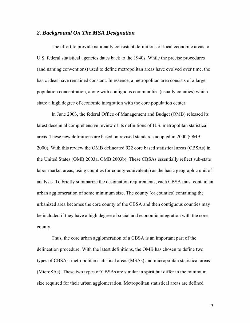
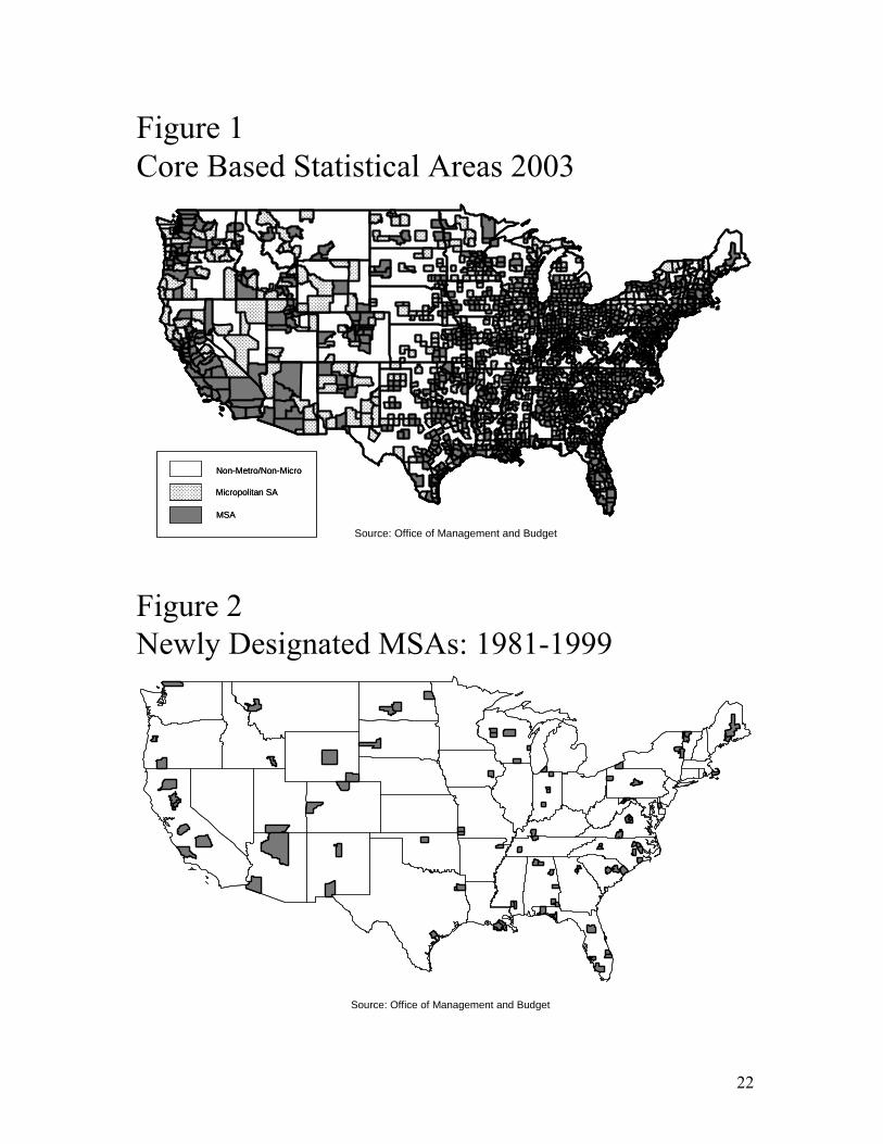
are 1,378 counties still classified as non-metropolitan/non-micropolitan. Figure 1 shows
the geographic distribution of MSAs and MicroSAs for the U.S. Note that MSAs are
particularly concentrated in the Northeast, while MicroSAs are distributed across the
South, Midwest, and West.
[FIGURE 1 ABOUT HERE]

5
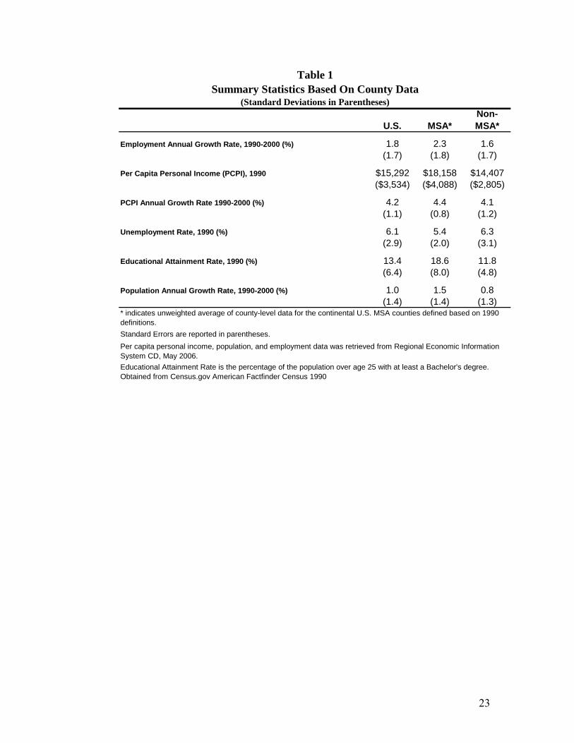
Further, income levels, unemployment rates, educational attainment rates, and
employment growth rates differ across metropolitan and non-metropolitan counties, as
Table 1 shows using 1990 MSA definitions for the continental U.S. Indeed, the average
level of per capita personal income for the metropolitan counties was $18,158, compared
to $14,407 for non-metropolitan counties. Unemployment rates were lower in
metropolitan counties, averaging 5.4%, compared to 6.3% for non-metropolitan counties
in 1990. Educational attainment, measured by the share of residents age 25 and older with
a bachelor’s degree or better, were higher in metropolitan counties, at 18.6%, than in non-
metropolitan counties, at 11.8%. Table 1 also shows that on average metropolitan
counties grew faster than non-metropolitan counties during the 1990s, posting higher
employment, population, and per capita personal income growth rates during the decade.
These results are widely known and may have given some observers the impression that
the MSA designation itself improves economic growth.
[TABLE 1 ABOUT HERE]
3. The MSA Designation And Growth
The metropolitan growth advantage arises from the geographic and socio-
economic characteristics of the MSAs and their residents. For instance, MSAs likely
attract more investment in productive inputs, like human capital, plant and equipment,
and perhaps even public infrastructure capital, which standard growth models suggest
will generate faster economic gains (Crihfield and Panggabean (1995), Glaeser, et. al.
(1995), Duffy-Deno and Eberts (1991)). The literature has become increasingly focused
on the importance of human capital in metropolitan growth (Glaeser and Saiz (2004)).
Cities and metropolitan areas also have the advantage of agglomeration economies which

6
reward the large and dense concentrations of people and firms within a labor market
(Glaeser, et.al (1992)).
Thus, the metropolitan growth advantage would exist whether or not the OMB
produced a list of MSAs. However, the possibility remains that the designation of a
county or group of counties as an MSA may on its own spur growth. Indeed, this is a
claim often made by local officials. These claims are commonly linked to three main
considerations which are affected by the MSA designation.
First, the urbanized area designation, which is linked to the MSA designation,
changes the way in which certain federal funds are distributed and can change the amount
of federal funds which are distributed to a region. Second, the MSA designation may
increase the amount and detail of economic information provided by federal and state
statistical agencies on the region. Third, the MSA designation may raise the marketing
profile of the region, particularly with respect to national or multi-state site selection
searches. Each of these impacts has been cited in professional site selection periodicals
and in the popular press during our period of interest. For examples, see Herbers (1980),
Carlson (1981), Carlson (1982), Herbers (1981), El Nasser and Glamser (1996), Rhodes
(2002), Ruffini (2003), and McCurry (2003).1
With respect to federal funding, there are two main funding sources that are
frequently cited as being affected by the MSA designation: federal transportation and
highway funds, as well as Housing and Urban Development (HUD) funds through the
Community Development Block Grant (CDBG) program.2 These two programs currently
make use of the urbanized area designation (and which are thus linked to the MSA
designation) when allocating funds. For instance, current federal transportation

7
legislation (Transportation Equity Act for the 21st Century (TEA-21)) requires that a new
urbanized area form a Metropolitan Planning Organization (MPO) to formalize and
implement a continuing planning process for the local area. Federal funds are provided to
states to fund MPO activities. However, the designation of a new urbanized area does not
automatically increase the funding available to states for this purpose.
More generally, some transportation funding is allocated based on the urbanized
area designation, for example mass transportation grants based on the Federal Transit
Administration (FTA) Urbanized Area Formula Program (49 USC 5307). However, it is
important to keep in mind that not all of the funds available to a new urbanized area
under the FTA Urbanized Area Formula will be new to the region, since regions that do
not qualify as urbanized areas are eligible for funds through the FTA Formula Grants for
Other Than Urbanized Areas (49 USC 5311). It is also important to note that funds
obtained under the FTA Urbanized Area Formula often involve a state match to the
federal funding and that the reporting and administrative requirements on urbanized areas
can be higher than for non-urbanized areas. See Zeilinger (2002) for more details on the
impact of the urbanized area designation on current FTA funding.
Federal Housing and Urban Development (HUD) funds, through the 1974
Community Development Block Grant (CDBG) program, are distributed to states and
local communities in order to provide services, create jobs, and expand business
opportunities for economically vulnerable populations. These funds are made available to
entitlement communities (which include central cities of MSAs (urbanized areas), cities
within MSAs with population of 50,000 or more, and counties within MSAs with
population of 200,000 or more, excluding those in entitled cities) and to states based on a
8
formula using population, poverty, age of the housing stock, and other characteristics
related to need. States, in turn, distribute funds to smaller, non-entitlement localities. In
this case, new urbanized areas gain access to CDBG funds by direct application to HUD.
Localities that have not attained urbanized area status must compete with other similarly
sized localities for CDBG funds allocated to the state. A city attaining urbanized area
status may or may not acquire more funds through direct application to HUD than
through state channels.
Finally, the attainment of urbanized are status can also reduce federal funding to
regions, as they become ineligible for funding through sources specifically designed to
spur rural economic development. This includes some programs administered by USDA
Rural Development, including Guaranteed Business and Industry (B&I) Loans, Rural
Business Enterprise Grants, Rural Business Opportunity Grants.
The second impact of the MSA designation which is often cited, and the one for
which it was specifically designed, is an increase in socio-economic data published by
federal agencies. The MSA designation may increase the amount of information available
for a region, over and above the data that could be computed simply by summing the
component counties. This is because the aggregation of counties to the MSA level may
allow the statistical agency to report more industry detail, without violating
confidentiality requirements.3 Further, publishing data at the MSA level may ease the
computational burden on novice researchers attempting to learn more about a multi-
county region. Overall, increasing the socio-economic information available for a region
might translate into improved decision-making and planning by public and private
entities, which might improve MSA growth.
9
Finally, one of the expected benefits of the MSA designation is that it may raise
the marketing profile of the region. One variant of this tale is the belief that site selection
consultants frequently start their search with a list of MSAs. Then the list is winnowed
down, based on analysis of the business climate, wage structure, educational
characteristics, transportations linkages, among other factors, to a few surviving MSAs,
one of which is finally chosen for the new plant location. Obviously, by attaining MSA
status, a region increases its odds of making the final cut.
Thus, we have three commonly cited reasons to suspect that the MSA designation
may impact a regional economy. It is typically taken for granted by local officials that
these impacts add up to a significantly positive impact on regional growth. However,
there is controversy on this score with respect to public capital investment, of which mass
transit and highway spending, excluding maintenance, are a part. For instance, Crihfield
and Panggabean (1995) and Glaeser et. al. (1995) find little impact of public capital
spending on metropolitan area growth during the 1960-1990 period. Further, several
researchers find that street-highway construction tends to raise the level of economic
activity in the county the road passes through, although this appears to be at the cost of
neighboring counties (Chandra and Thompson (2000), Rephann and Isserman (1994),
Boarnet (1998)). These offsetting impacts leave regional growth little changed.
We know of no empirical results on possible metropolitan-level growth impacts
of CDBG funds, but Glaeser et.al. (1995) find little correlation between
intergovernmental revenues and city growth during the 1960-1990 period. HUD
assessments to date, reported in Walker et.al. (2002), focus on neighborhood-level
impacts for 17 cities and find positive impacts of “substantial” CDBG investments. We

10
know of no previous empirical research on the metropolitan growth impacts of the
marketing of regions or of the increased data availability.
Our purpose in the next section is to use the MSA designations from OMB in the
early 1980s and 1990s to test the hypothesis that the MSA designation improves regional
growth. We will measure this growth using three indicators commonly used in the
literature on metropolitan economic performance: population, per capita personal income,
and employment.
4. Data And Empirical Results
The Office of Management and Budget (OMB) publishes lists of metropolitan
statistical areas and their component counties. We obtained these lists for the years
between 1981 and 1999. We focus our analysis on newly designated MSAs in the
continental U.S. that were published as such during this period, due to constraints on the
length of our time-series data. Further, we focus on MSAs that represent the transition of
formerly non-metropolitan counties to MSAs, on the grounds that this will provide the
clearest test of the hypothesis. In other words, we exclude MSAs that were formed by
splitting (in part or in whole) previously existing MSAs. MSA designations are released
in the middle of the year (in either June or July). As a result, we assume that the growth
impacts of the designation will begin the year following the public announcement. For
instance, for metropolitan areas that were announced in June of 1981, the proposed year
of structural change is 1982. Table 2 contains the final list of 70 MSAs designated after
1980 and their year of designation and Figure 2 shows the geographic distribution of
these MSAs.
[FIGURE 2 ABOUT HERE]
11
[TABLE 2 ABOUT HERE]
Upon finalizing the list of new MSAs between 1981 and 1999, we gathered
county-level data for those MSAs from the Bureau of Economic Analysis (BEA)
Regional Economic Information System CD-Rom for the 1969 to 2003 period. We
obtained data on personal income, population, and full- and part-time employment for all
counties that were part of newly designated MSAs. 4 We then aggregated the county data
for each MSA follows:
,1
,, ∑=
=C
ititMSA EmploymentEmployment
,1
,, ∑=
=C
ititMSA PopulationPopulation
,
1,
1,
,
∑
∑
=
== C
iti
C
iti
tMSA
Population
comePersonalInPCPI
where i indexes counties included in the MSA and C indicates the total number of
counties within the MSA.
4.1 Average Growth Rates Before And After The MSA Designation
Since it is likely that metropolitan area performance is influenced by the
economic performance of the nation, we express the metropolitan data relative to the
nation and then compute annual growth rates relative to the U.S. as follows:
( ) ( )[ ],lnln ,,, tUStMSAtMSA EmploymentEmploymentREGrowth −∆=
( ) ( )[ ],lnln ,,, tUStMSAtMSA PopulationPopulationRPGrowth −∆=
( ) ( )[ ],lnln ,,, tUStMSAtMSA PCPIPCPIhRPCPIGrowt −∆=
12
where ∆ is the first difference operator. We begin by examining the means of the
relative growth rates (REGrowthMSA,t, RPGrowthMSA,t, and RPCPIGrowthMSA,t) before and
after the MSA designation. If the MSA designation spurs economic activity, then we
expect to see significantly faster relative income, employment, and population growth
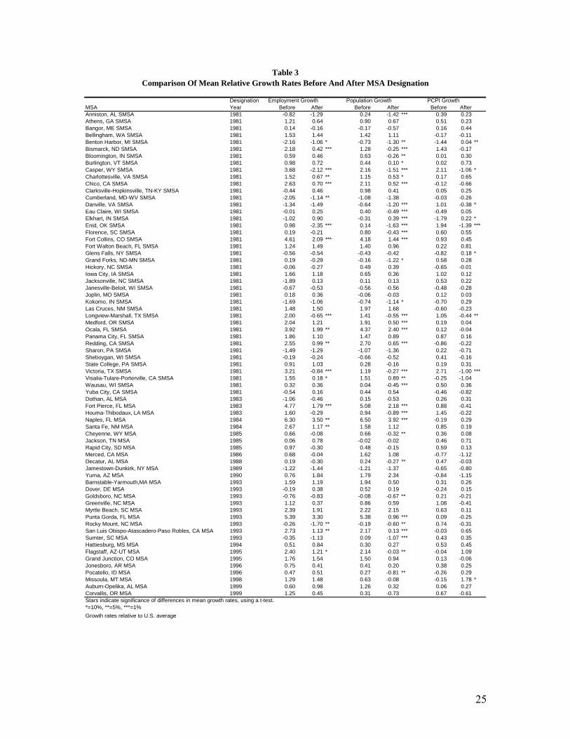
after the designation year than before the designation year. Table 3 summarizes the mean
relative growth rates before and after designation for the 70 MSAs we consider, as well
as the results of a t-test test for significant differences across mean growth rates before
and after designation.
[TABLE 3 ABOUT HERE]
As Table 3 shows, there were 24 cases in which mean relative employment
growth was faster after designation, but only two instances in which relative employment
growth was significantly faster (at the 10% level) after the designation (Benton Harbor,
Michigan and Cumberland, Maryland). However, there were 46 cases in which mean
employment growth was slower after the designation and in 17 of those cases the
differences was significant at the 10% level.
For population growth, there were seven cases in which growth was faster after
designation and one instance in which growth was significantly faster at the 10% level
(Elkhart, Indiana). In contrast, we find 63 cases in which mean growth was slower after
designation, with 34 of these differences significant at the 10% level.
Finally, for relative per capita personal income growth, there were 26 cases in
which growth was faster after designation, but again, only four cases in which growth
was significantly faster (Benton Harbor, Michigan; Elkhart, Indiana; Glen Falls, New
13
York; and Missoula, Montana). On the other hand, there were 44 cases with slower
growth after designation, with five of these significant at the 10% level.
Overall, the results suggest little positive growth impact arising from the MSA
designation. Indeed, we more often observe relative employment, population, and per
capita personal income growth slowing significantly after designation. However, it is
important to note that we have relatively few degrees of freedom to use in our t-test for a
difference in means. We would feel more confident with 25-30 observations before and
after designation, but unfortunately, this is precluded by our dataset.
4.2 Econometric Tests of Structural Change
In order to check the robustness of our initial results, we carry out an econometric
test for the growth impact of the MSA designation: the Chow forecast test for structural
change. The Chow forecast test consists of two growth rate regressions.5 The first
regression uses data for the entire period (1969-2003). The second regression uses data
for the longer of the two sub-periods (before designation or after designation). The null
hypothesis of the Chow forecast test is that the parameters are equal across the two
regressions. In our context, the null hypothesis implies that the MSA designation has no
impact on MSA growth. We prefer the Chow forecast test over the traditional Chow
breakpoint test because, for several MSAs, there are very few observations available after
the MSA designation. Such a degrees-of-freedom problem will prevent the shorter period
from being tested using the standard Chow breakpoint test.
We implement the Chow forecast test using the following specification:
,,1, ttustMSA XX εβα +∆+=∆

14
where XMSA,t (Xus,t) is the log of the MSA (U.S.) variable of interest (employment,
population, or per capita personal income), and εt is the residual. We test the residuals for
serial correlation using an LM test and where the null hypothesis of no serial correlation
is rejected, we add up to two lags of the dependent variable. Summary statistics for the
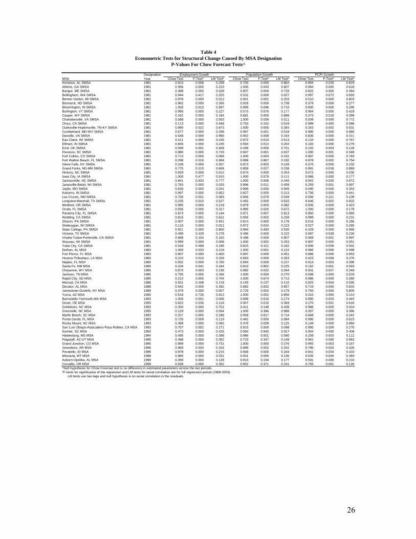
full regression and the results of the Chow forecast test are summarized in Table 4.
[TABLE 4 ABOUT HERE]
Overall, we find little evidence of structural breaks associated (in time) with the
MSA designation. For instance we find evidence of a structural break in three
employment series (Enid, Oklahoma; Sharon, Pennsylvania; and Jamestown-Dunkirk,
New York), zero population series, and five per capita personal income series (Hickory,
North Carolina; Joplin, Missouri; Sharon, Pennsylvania; Victoria, Texas; and Missoula,
Montana). There was one case (Jamestown-Dunkirk, New York) of significantly higher
average employment growth after MSA designation. On the other hand, Sharon,
Pennsylvania experienced significantly lower average employment growth after
designation. Similarly, two MSAs (Hickory, North Carolina and Joplin, Missouri)
experienced significantly higher real per capita personal income growth after being
classified as a metropolitan area. Victoria, Texas actually had higher income growth prior
to the designation. Overall, the results of our econometric tests for structural breaks based
on the MSA designation do not provide much evidence in favor of significant differences
before and after the designation.
4.3 Quasi-Experimental Matching
Our tests so far require that the MSA designation impact meet a high standard:
that the impact on growth is large enough to influence average growth over a long period
15
of time. The quasi-experimental matching approach detailed in Isserman and Merrifield
(1987) and expanded upon in Rephann and Isserman (1994), allows for a more flexible
and sensitive test of the impact of the MSA designation. This method entails conducting
pre-tests and post-tests on growth rate differences between treatment regions and control
regions. In this paper, the treatment is MSA designation, and the treatment regions are the
newly designated MSAs. The control regions are elements selected from the set of 2,192
nonmetropolitan counties. Each new MSA is optimally paired with a single control
county based on the two regions’ level of similarity to each other during the time period
just prior to the MSA designation. The intuition is that, provided the treatment and
control regions did not have significant pre-designation growth rate differences, then
significant post-designation growth rate differences indicate that MSA designation (the
treatment) has a significant effect on a region’s growth.
The first step, control county selection, was achieved with the use of 18 selection
variables, or calipers, that are listed in Table 5. For each time-variant caliper, we compare
the average annual growth rates for each treatment region and each potential control
county for the five years prior to the treatment region’s MSA designation.6 So, for an
MSA designated in 1981, we calculate the cumulative growth rate for each caliper for the
years 1976 to 1980. The optimally matched control county is the one which has the least
cumulative difference between its calipers and those of the treatment region.
[TABLE 5 ABOUT HERE]
The formal process of finding the matching area first requires the calculation of a
Mahalanobis distance between (a) each of the 70 treatment counties and (b) each of the
16
2,192 non-metropolitan U.S. counties that both is not in our set of MSA counties and has
not been previously included in an existing MSA. This distance is calculated as follows:
( ) ( ) ( )iTiTiT XXRXXXXM −′−= −1,
where ( )iT XXM , is the scalar Mahalanobis distance between the treatment
region (T) and each potential control county (i), TX and iX are the respective 18 x 1
vectors of the selection variables for the treatment region and potential control county,
and 1−R is the 18 x 18 inverted variance-covariance matrix of the selected calipers for the
potential control counties.
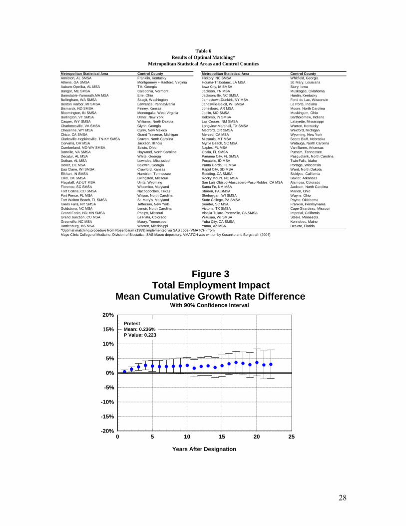
Final selection of control counties relies on the optimal matching procedure
described by Rosenbaum (1989). This procedure, analogous to solving a network flow
problem, ensures that one control county is assigned to a treatment MSA and that the sum
of the Mahalanobis distances is minimized. Implementation was completed using a SAS
optimization program written by Kosanke and Bergstralh (2004). The final list of
optimally matched pairs is displayed in Table 6.
[TABLE 6 ABOUT HERE]
Once the potential control counties were identified, the next step requires testing
the pre-MSA designation growth rates for the employment, personal income, and
population data series. Provided that the treatment regions and potential control counties
had similar rates of pre-designation growth, the pairs of regions can then be retained for
use in the post-test comparisons.
First, for each of our performance measures (population, per capita personal
income, employment) we compute average annual growth rate differences for the
matched pairs during the pre-designation period. Then we employ a t-test to determine if
17
the average of the growth rate differences across the 70 matched pairs is significantly
different from zero. Our initial pre-tests are passed at the 10% significance level for per
capita personal income, but not for population or employment. Our solution to this
problem is to exclude matched pairs with large growth rate differences until the pre-test is
passed. For employment, this procedure results in the deletion of the Fort Pierce and
Naples Florida MSAs. For population, we drop the Fort Pierce, Naples, and Punta Gorda
MSAs in Florida, as well as the Fort Collins Colorado, Merced California, Auburn-
Opelika Alabama, Redding California, San Luis Obispo California, and Missoula
Montana MSAs.
[TABLE 5 ABOUT HERE]
With our matched pairs that pass the pre-test, we then carried out post-tests of the
mean cumulative growth rate differences for the employment, personal income, and
population data series. For each year post-designation, each series’ mean cumulative
growth rate difference was calculated as follows:
( )j
n
i
Cjt
Tjt
jt n
rrD
j
∑=
−= 1
Where jtD is the mean difference in cumulative growth rates for jn -pairs of
regions, and Tjtr and C
jtr are the cumulative growth rates of the treatment and control
regions, respectively, for each series-j between the year of MSA designation and t-years
beyond. Our results for employment, personal income, and population are portrayed in
Figure 3, Figure 4, and Figure 5, respectively.
[FIGURE 3 ABOUT HERE]

18
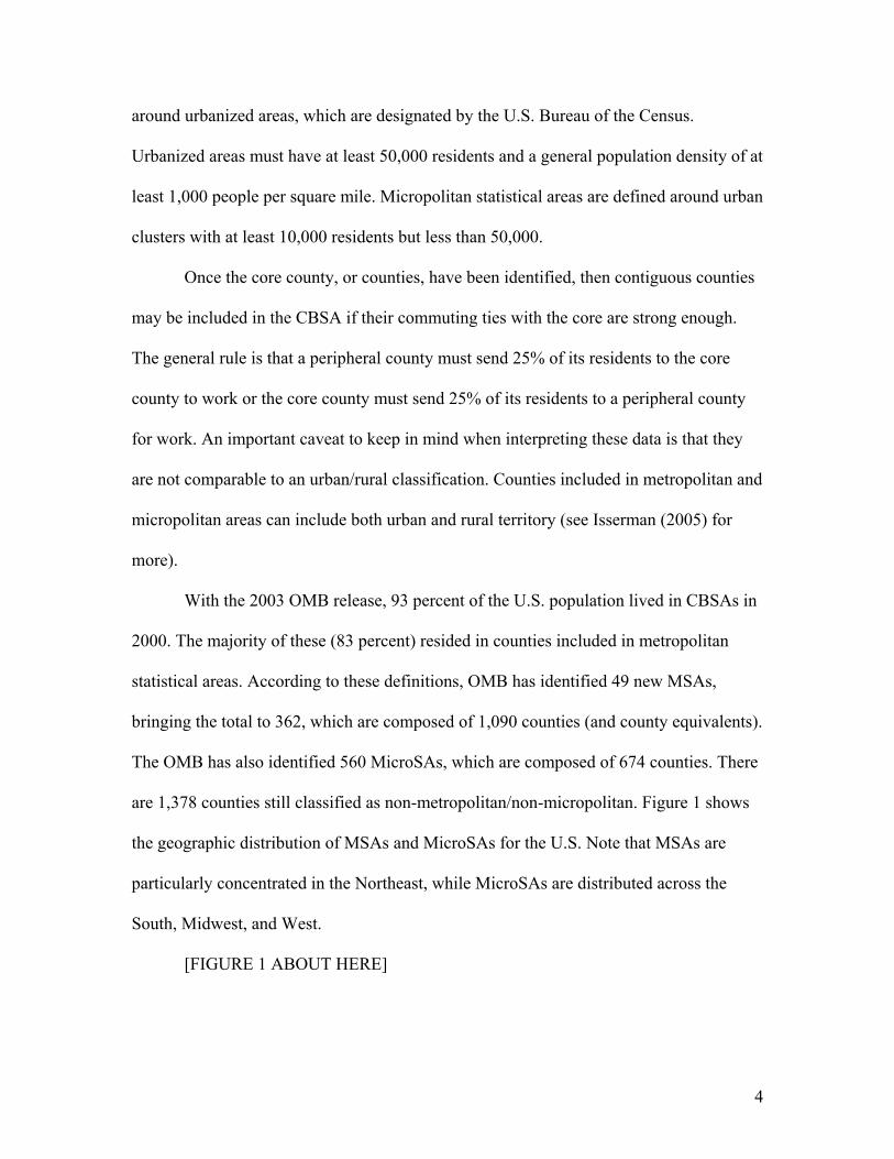
As shown in Figure 3, the MSA designation does not have a significant (at the
10% level) impact employment growth in the long run. However, the figure does show a
short-term, positive impact between two and six years post-designation, which indicates a
possible transitory impact of the MSA designation. The magnitude of the growth impact
reaches a peak at four years after designation of 2.6%. Thus, for employment growth,
local officials may have observed a short-term employment impact that is present in the
data.
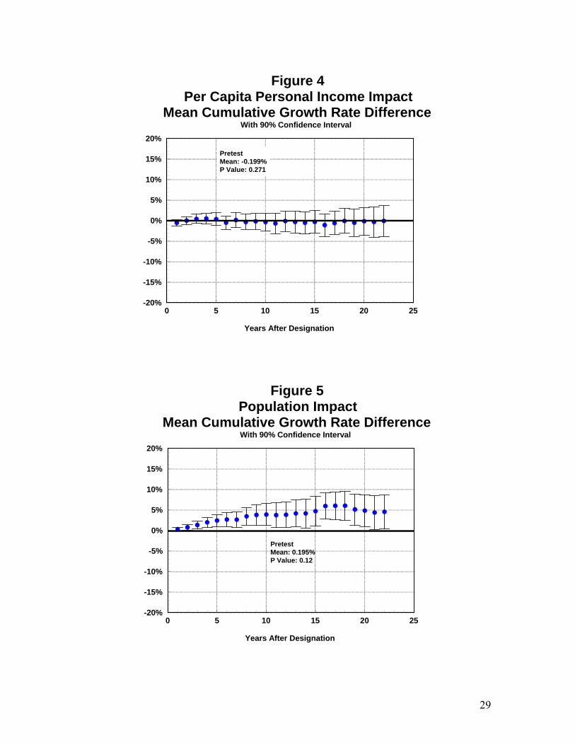
[FIGURE 4 ABOUT HERE]
Figure 4, on cumulative personal income growth, provides less support for the
hypothesis that MSA designation affects regional growth. For this series, all 70 MSAs
remained in the sample and average growth rate differences are never significantly
different from zero at the 10% level and the mean growth rate differences tend to be very
close to zero. This is an important result, because per capita income should be a key
target variable for policymakers looking to raise the standard of living of a region.
[FIGURE 5 ABOUT HERE]
The strongest results in support of higher post-MSA designation growth are found
in the population series, shown in Figure 5. We find statistically significant long-run
growth rate differences that grow over time to a peak of 6.0% 16-18 years after
designation. While the results indicate that there is a positive effect of MSA designation
on county population growth, they are weakened by the fact that 10 of the 70 MSA
counties (and their twins) were eliminated due to poor pre-test matching. Also,
population growth may show the strongest impact because population size is a key

19
consideration in the MSA designation. Thus, it may be that strong population growth
causes the MSA designation, and not the other way around.
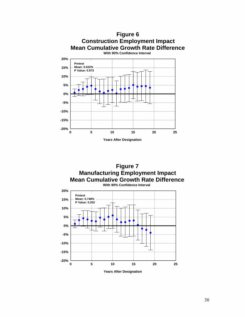
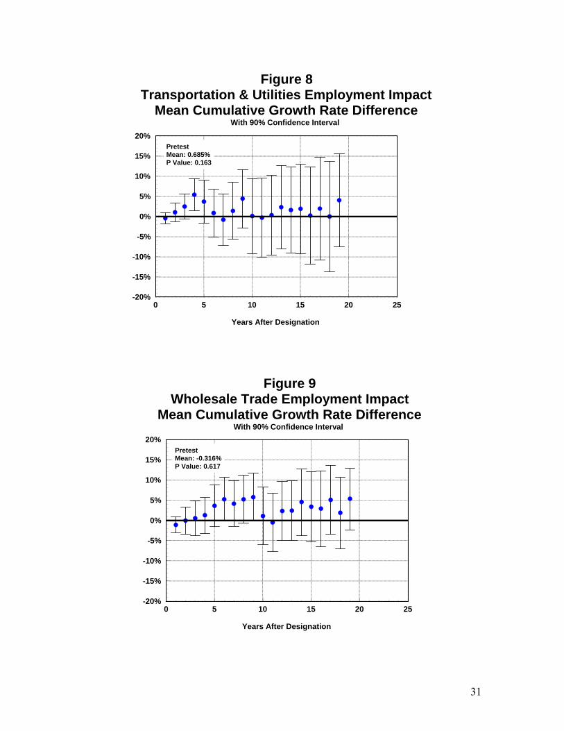
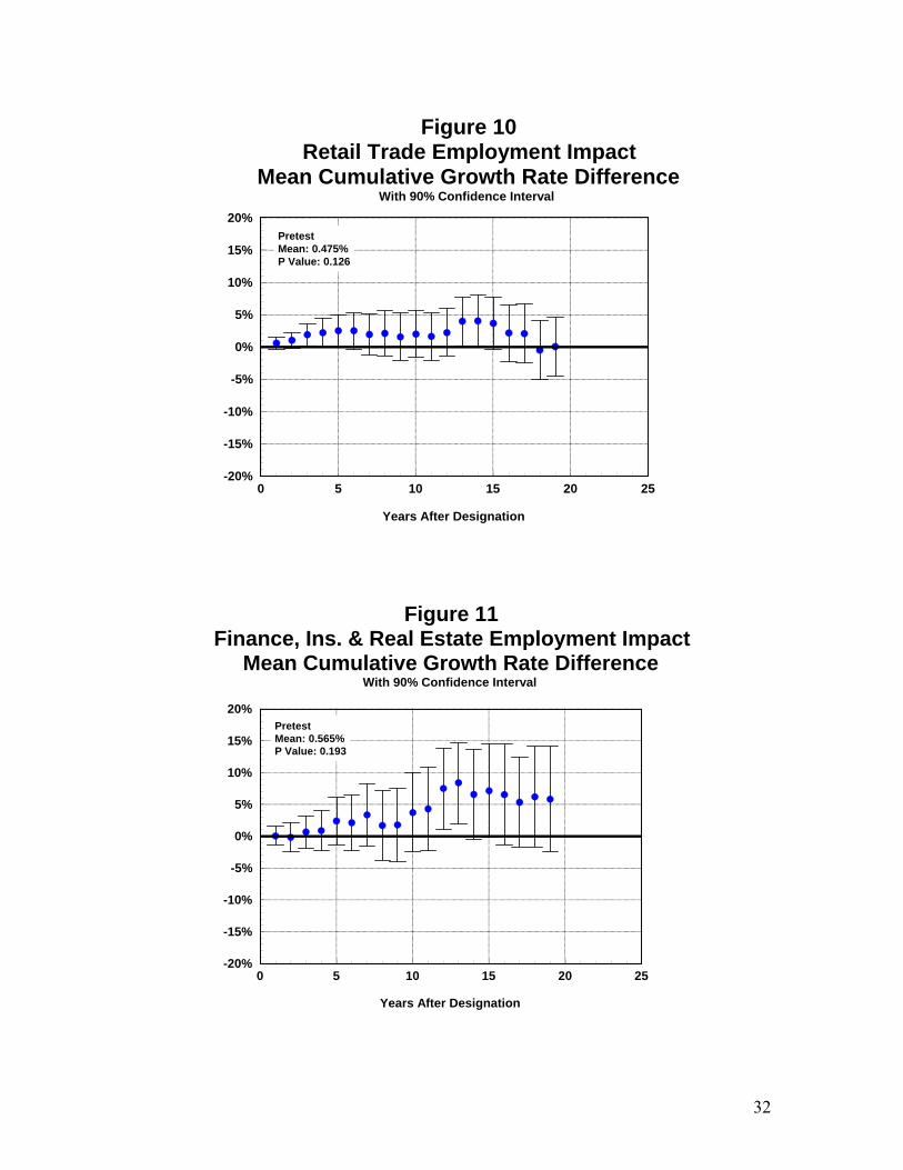
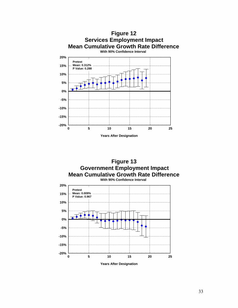
Figures 6 through 13 summarize our quasi-experimental results for eight SIC
sectors: construction; manufacturing; transportation and utilities; wholesale trade; retail
trade; finance insurance and real estate; services; and government. The focus on industry-
level data (classified by SIC) means that our time period ends in 2000, with the transition
from SIC to NAICS. We do not report results for agriculture and mining because data is
often suppressed due to federal disclosure rules. As the figures show, we find significant
impacts for several sectors, including transportation and utilities; retail trade; finance
insurance and real estate; services; and government. For transportation and utilities; retail
trade; and government; the impacts are primarily short-run, because they die out within
six years. For services we find much more persistent growth impacts, which become
significantly positive after two years and remain positive through the test interval. The
growth rate impact for services rises over time to a peak of 8.0% 17 years after
designation. Employment growth impacts for finance, insurance, and real estate are
insignificant in most years, but become significantly different from zero for the twelfth
and thirteenth year after designation.
Overall, our quasi-experimental results provide a more subtle test of the impact of
the MSA designation. These results suggest that there is a modest short-run impact on
employment growth in regions receiving the MSA designation, with those employment
impacts concentrated in services; government; transportation and utilities; retail trade;
and finance, insurance, and real estate. We find more substantial longer-term impacts on
population growth. Finally, the tests show no impact of the MSA designation on per
20
capita personal income, perhaps the most important measure of a region’s standard of
living.
5. Implications and Conclusion
Our empirical work suggests that local officials in non-metropolitan counties
should be wary of assertions that the MSA designation spurs economic growth, at least in
the case of long-run aggregate employment and per capita personal income growth. We
find little difference in mean relative growth rates before and after the MSA designation
and little support from Chow tests for structural breaks for all three indicators considered.
Our quasi-experimental results detect a statistically significant, but short term, impact
with respect to aggregate employment growth. We also disaggregate employment by
industry and find short-run employment growth impacts for transportation and utilities;
retail trade; and government. We find longer-term impacts for services, as well as
finance, insurance, and real estate. The employment growth results suggest that there may
be some short-run value to the MSA designation in terms of increasing the visibility of
the region.
However, the MSA designation does not significantly spur per capita income
growth, which suggests that local policymakers should not expend scarce resources in
pursuit of the designation. In contrast, population growth is significantly and positively
affected by MSA designation; but because this series already plays a role in the MSA
designation process, we are less confident in the interpretation of these results. In
summary, our results suggest that the MSA designation does not spur longer-term growth
in formerly non-metropolitan regions in terms of aggregate employment or per capita
personal income, but may play a role in population growth.
21
Finally, our results suggest that local officials in non-metropolitan regions should
primarily focus their efforts on improving the regional characteristics that do influence
long-term growth, particularly human capital. Beeson, et. al. (2001), Hammond and
Thompson (2005), and Hammond (2006), show that investment in human capital remains
an important determinant of economic growth, even for non-metropolitan regions.
22
Figure 1Core Based Statistical Areas 2003
Non-Metro/Non-Micro
Micropolitan SA
MSA
Non-Metro/Non-Micro
Micropolitan SA
MSA
Source: Office of Management and Budget
Figure 2Newly Designated MSAs: 1981-1999
Source: Office of Management and Budget
23
U.S. MSA*Non-MSA*
Employment Annual Growth Rate, 1990-2000 (%) 1.8 2.3 1.6(1.7) (1.8) (1.7)
Per Capita Personal Income (PCPI), 1990 $15,292 $18,158 $14,407($3,534) ($4,088) ($2,805)
PCPI Annual Growth Rate 1990-2000 (%) 4.2 4.4 4.1(1.1) (0.8) (1.2)
Unemployment Rate, 1990 (%) 6.1 5.4 6.3(2.9) (2.0) (3.1)
Educational Attainment Rate, 1990 (%) 13.4 18.6 11.8(6.4) (8.0) (4.8)
Population Annual Growth Rate, 1990-2000 (%) 1.0 1.5 0.8(1.4) (1.4) (1.3)
Table 1Summary Statistics Based On County Data
(Standard Deviations in Parentheses)
* indicates unweighted average of county-level data for the continental U.S. MSA counties defined based on 1990 definitions.Standard Errors are reported in parentheses.Per capita personal income, population, and employment data was retrieved from Regional Economic Information System CD, May 2006.Educational Attainment Rate is the percentage of the population over age 25 with at least a Bachelor's degree. Obtained from Census.gov American Factfinder Census 1990

24
#Designation Year MSA #
Designation Year MSA
1 1981 Anniston, AL SMSA 36 1981 Sheboygan, WI SMSA2 1981 Athens, GA SMSA 37 1981 State College, PA SMSA3 1981 Bangor, ME SMSA 38 1981 Victoria, TX SMSA4 1981 Bellingham, WA SMSA 39 1981 Visalia-Tulare-Porterville, CA SMSA5 1981 Benton Harbor, MI SMSA 40 1981 Wausau, WI SMSA6 1981 Bismarck, ND SMSA 41 1981 Yuba City, CA SMSA7 1981 Bloomington, IN SMSA 42 1983 Dothan, AL MSA8 1981 Burlington, VT SMSA 43 1983 Fort Pierce, FL MSA9 1981 Casper, WY SMSA 44 1983 Houma-Thibodaux, LA MSA10 1981 Charlottesville, VA SMSA 45 1984 Naples, FL MSA11 1981 Chico, CA SMSA 46 1984 Santa Fe, NM MSA12 1981 Clarksville-Hopkinsville, TN-KY SMSA 47 1985 Cheyenne, WY MSA13 1981 Cumberland, MD-WV SMSA 48 1985 Jackson, TN MSA14 1981 Danville, VA SMSA 49 1985 Rapid City, SD MSA15 1981 Eau Claire, WI SMSA 50 1986 Merced, CA MSA16 1981 Elkhart, IN SMSA 51 1988 Decatur, AL MSA17 1981 Enid, OK SMSA 52 1989 Jamestown-Dunkirk, NY MSA18 1981 Florence, SC SMSA 53 1990 Yuma, AZ MSA19 1981 Fort Collins, CO SMSA 54 1993 Dover, DE MSA20 1981 Fort Walton Beach, FL SMSA 55 1993 Goldsboro, NC MSA21 1981 Glens Falls, NY SMSA 56 1993 Greenville, NC MSA22 1981 Grand Forks, ND-MN SMSA 57 1993 Myrtle Beach, SC MSA23 1981 Hickory, NC SMSA 58 1993 Punta Gorda, FL MSA24 1981 Iowa City, IA SMSA 59 1993 Rocky Mount, NC MSA25 1981 Jacksonville, NC SMSA 60 1993 San Luis Obispo-Atascadero-Paso Robles, CA MSA26 1981 Janesville-Beloit, WI SMSA 61 1993 Sumter, SC MSA27 1981 Joplin, MO SMSA 62 1993 Barnstable-Yarmouth, MA MSA28 1981 Kokomo, IN SMSA 63 1994 Hattiesburg, MS MSA29 1981 Las Cruces, NM SMSA 64 1995 Flagstaff, AZ-UT MSA30 1981 Longview-Marshall, TX SMSA 65 1995 Grand Junction, CO MSA31 1981 Medford, OR SMSA 66 1996 Jonesboro, AR MSA32 1981 Ocala, FL SMSA 67 1996 Pocatello, ID MSA33 1981 Panama City, FL SMSA 68 1998 Missoula, MT MSA34 1981 Redding, CA SMSA 69 1999 Auburn-Opelika, AL MSA35 1981 Sharon, PA SMSA 70 1999 Corvallis, OR MSASource: U.S. Census Bureau, Historical Metropolitan Area Definitions,http://www.census.gov/population/www/estimates/pastmetro.html^Excluding MSAs that were formed by splitting (in part or in whole) previously existing MSAs.
Table 2Newly Designated MSAs During 1981-1999 Period^
25
DesignationMSA Year Before After Before After Before AfterAnniston, AL SMSA 1981 -0.82 -1.29 0.24 -1.42 *** 0.39 0.23Athens, GA SMSA 1981 1.21 0.64 0.90 0.67 0.51 0.23Bangor, ME SMSA 1981 0.14 -0.16 -0.17 -0.57 0.16 0.44Bellingham, WA SMSA 1981 1.53 1.44 1.42 1.11 -0.17 -0.11Benton Harbor, MI SMSA 1981 -2.16 -1.06 * -0.73 -1.30 ** -1.44 0.04 **Bismarck, ND SMSA 1981 2.18 0.42 *** 1.28 -0.25 *** 1.43 -0.17Bloomington, IN SMSA 1981 0.59 0.46 0.63 -0.26 ** 0.01 0.30Burlington, VT SMSA 1981 0.98 0.72 0.44 0.10 * 0.02 0.73Casper, WY SMSA 1981 3.68 -2.12 *** 2.16 -1.51 *** 2.11 -1.06 *Charlottesville, VA SMSA 1981 1.52 0.67 ** 1.15 0.53 * 0.17 0.65Chico, CA SMSA 1981 2.63 0.70 *** 2.11 0.52 *** -0.12 -0.66Clarksville-Hopkinsville, TN-KY SMSA 1981 -0.44 0.46 0.98 0.41 0.05 0.25Cumberland, MD-WV SMSA 1981 -2.05 -1.14 ** -1.08 -1.38 -0.03 -0.26Danville, VA SMSA 1981 -1.34 -1.49 -0.64 -1.20 *** 1.01 -0.38 *Eau Claire, WI SMSA 1981 -0.01 0.25 0.40 -0.49 *** -0.49 0.05Elkhart, IN SMSA 1981 -1.02 0.90 -0.31 0.39 *** -1.79 0.22 *Enid, OK SMSA 1981 0.98 -2.35 *** 0.14 -1.63 *** 1.94 -1.39 ***Florence, SC SMSA 1981 0.19 -0.21 0.80 -0.43 *** 0.60 0.55Fort Collins, CO SMSA 1981 4.61 2.09 *** 4.18 1.44 *** 0.93 0.45Fort Walton Beach, FL SMSA 1981 1.24 1.49 1.40 0.96 0.22 0.81Glens Falls, NY SMSA 1981 -0.56 -0.54 -0.43 -0.42 -0.82 0.18 *Grand Forks, ND-MN SMSA 1981 0.19 -0.29 -0.16 -1.22 * 0.58 0.28Hickory, NC SMSA 1981 -0.06 -0.27 0.49 0.39 -0.65 -0.01Iowa City, IA SMSA 1981 1.66 1.18 0.65 0.36 1.02 0.12Jacksonville, NC SMSA 1981 -1.89 0.13 0.11 0.13 0.53 0.22Janesville-Beloit, WI SMSA 1981 -0.67 -0.53 -0.56 -0.56 -0.48 -0.28Joplin, MO SMSA 1981 0.18 0.36 -0.06 -0.03 0.12 0.03Kokomo, IN SMSA 1981 -1.69 -1.06 -0.74 -1.14 * -0.70 0.29Las Cruces, NM SMSA 1981 1.48 1.50 1.97 1.68 -0.60 -0.23Longview-Marshall, TX SMSA 1981 2.00 -0.65 *** 1.41 -0.55 *** 1.05 -0.44 **Medford, OR SMSA 1981 2.04 1.21 1.91 0.50 *** 0.19 0.04Ocala, FL SMSA 1981 3.92 1.99 ** 4.37 2.40 *** 0.12 -0.04Panama City, FL SMSA 1981 1.86 1.10 1.47 0.89 0.87 0.16Redding, CA SMSA 1981 2.55 0.99 ** 2.70 0.65 *** -0.86 -0.22Sharon, PA SMSA 1981 -1.49 -1.29 -1.07 -1.36 0.22 -0.71Sheboygan, WI SMSA 1981 -0.19 -0.24 -0.66 -0.52 0.41 -0.16State College, PA SMSA 1981 0.91 1.03 0.28 -0.16 0.19 0.31Victoria, TX SMSA 1981 3.21 -0.84 *** 1.19 -0.27 *** 2.71 -1.00 ***Visalia-Tulare-Porterville, CA SMSA 1981 1.55 0.18 * 1.51 0.89 ** -0.25 -1.04Wausau, WI SMSA 1981 0.32 0.36 0.04 -0.45 *** 0.50 0.36Yuba City, CA SMSA 1981 -0.54 0.16 0.44 0.54 -0.46 -0.82Dothan, AL MSA 1983 -1.06 -0.46 0.15 -0.53 0.26 0.31Fort Pierce, FL MSA 1983 4.77 1.79 *** 5.08 2.18 *** 0.88 -0.41Houma-Thibodaux, LA MSA 1983 1.60 -0.29 0.94 -0.89 *** 1.45 -0.22Naples, FL MSA 1984 6.30 3.50 ** 6.50 3.92 *** -0.19 0.29Santa Fe, NM MSA 1984 2.67 1.17 ** 1.58 1.12 0.85 0.19Cheyenne, WY MSA 1985 0.66 -0.08 0.66 -0.32 ** 0.36 0.08Jackson, TN MSA 1985 0.06 0.78 -0.02 -0.02 0.46 0.71Rapid City, SD MSA 1985 0.97 -0.30 0.48 -0.15 0.59 0.13Merced, CA MSA 1986 0.68 -0.04 1.62 1.08 -0.77 -1.12Decatur, AL MSA 1988 0.19 -0.30 0.24 -0.27 ** 0.47 -0.03Jamestown-Dunkirk, NY MSA 1989 -1.22 -1.44 -1.21 -1.37 -0.65 -0.80Yuma, AZ MSA 1990 0.76 1.84 1.79 2.34 -0.84 -1.15Barnstable-Yarmouth,MA MSA 1993 1.59 1.19 1.94 0.50 0.31 0.26Dover, DE MSA 1993 -0.19 0.38 0.52 0.19 -0.24 0.15Goldsboro, NC MSA 1993 -0.76 -0.83 -0.08 -0.67 ** 0.21 -0.21Greenville, NC MSA 1993 1.12 0.37 0.86 0.59 1.08 -0.41Myrtle Beach, SC MSA 1993 2.39 1.91 2.22 2.15 0.63 0.11Punta Gorda, FL MSA 1993 5.39 3.30 5.38 0.96 *** 0.09 -0.25Rocky Mount, NC MSA 1993 -0.26 -1.70 ** -0.19 -0.60 ** 0.74 -0.31San Luis Obispo-Atascadero-Paso Robles, CA MSA 1993 2.73 1.13 ** 2.17 0.13 *** -0.03 0.65Sumter, SC MSA 1993 -0.35 -1.13 0.09 -1.07 *** 0.43 0.35Hattiesburg, MS MSA 1994 0.51 0.84 0.30 0.27 0.53 0.45Flagstaff, AZ-UT MSA 1995 2.40 1.21 * 2.14 -0.03 ** -0.04 1.09Grand Junction, CO MSA 1995 1.76 1.54 1.50 0.94 0.13 -0.06Jonesboro, AR MSA 1996 0.75 0.41 0.41 0.20 0.38 0.25Pocatello, ID MSA 1996 0.47 0.51 0.27 -0.81 ** -0.26 0.29Missoula, MT MSA 1998 1.29 1.48 0.63 -0.08 -0.15 1.78 *Auburn-Opelika, AL MSA 1999 0.60 0.98 1.26 0.32 0.06 0.27Corvallis, OR MSA 1999 1.25 0.45 0.31 -0.73 0.67 -0.61Stars indicate significance of differences in mean growth rates, using a t-test.*=10%, **=5%, ***=1%Growth rates relative to U.S. average
Comparison Of Mean Relative Growth Rates Before And After MSA DesignationTable 3
Employment Growth Population Growth PCPI Growth
26
DesignationMSA Year Chow Test F-Test* LM Test* Chow Test F-Test* LM Test* Chow Test F-Test* LM Test*Anniston, AL SMSA 1981 0.910 0.006 0.258 0.700 0.059 0.864 0.994 0.035 0.819Athens, GA SMSA 1981 0.956 0.000 0.223 1.000 0.043 0.607 0.984 0.000 0.618Bangor, ME SMSA 1981 0.388 0.000 0.028 0.807 0.000 0.729 0.832 0.000 0.384Bellingham, WA SMSA 1981 0.944 0.417 0.203 0.532 0.000 0.027 0.997 0.072 0.693Benton Harbor, MI SMSA 1981 0.978 0.000 0.012 0.941 0.001 0.203 0.510 0.000 0.803Bismarck, ND SMSA 1981 0.962 0.000 0.356 0.928 0.000 0.738 0.379 0.009 0.277Bloomington, IN SMSA 1981 1.000 0.010 0.897 0.999 0.096 0.710 0.800 0.000 0.295Burlington, VT SMSA 1981 0.990 0.000 0.227 0.575 0.076 0.177 0.964 0.000 0.419Casper, WY SMSA 1981 0.162 0.000 0.184 0.681 0.000 0.898 0.373 0.018 0.399Charlottesville, VA SMSA 1981 0.588 0.000 0.503 1.000 0.036 0.511 0.509 0.000 0.772Chico, CA SMSA 1981 0.113 0.000 0.468 0.753 0.162 0.518 0.999 0.000 0.086Clarksville-Hopkinsville, TN-KY SMSA 1981 0.990 0.022 0.873 1.000 0.655 0.284 0.263 0.002 0.531Cumberland, MD-WV SMSA 1981 0.677 0.000 0.299 0.997 0.001 0.518 0.985 0.000 0.880Danville, VA SMSA 1981 0.548 0.000 0.990 0.942 0.008 0.164 0.835 0.000 0.411Eau Claire, WI SMSA 1981 0.411 0.000 0.435 0.972 0.010 0.513 0.134 0.000 0.767Elkhart, IN SMSA 1981 0.846 0.000 0.245 0.594 0.014 0.204 0.183 0.000 0.279Enid, OK SMSA 1981 0.099 0.001 0.409 0.438 0.000 0.701 0.102 0.004 0.128Florence, SC SMSA 1981 0.980 0.000 0.733 0.947 0.001 0.637 1.000 0.001 0.348Fort Collins, CO SMSA 1981 0.713 0.000 0.066 1.000 0.004 0.191 0.997 0.000 0.783Fort Walton Beach, FL SMSA 1981 0.298 0.016 0.904 0.999 0.867 0.192 0.978 0.002 0.754Glens Falls, NY SMSA 1981 0.108 0.000 0.507 0.973 0.003 0.128 0.376 0.000 0.232Grand Forks, ND-MN SMSA 1981 0.775 0.315 0.608 0.859 0.027 0.238 0.991 0.018 0.869Hickory, NC SMSA 1981 0.929 0.000 0.012 0.974 0.000 0.353 0.072 0.000 0.030Iowa City, IA SMSA 1981 1.000 0.477 0.910 1.000 0.579 0.111 0.986 0.000 0.177Jacksonville, NC SMSA 1981 0.841 0.933 0.777 1.000 0.006 0.440 0.942 0.030 0.972Janesville-Beloit, WI SMSA 1981 0.783 0.000 0.033 0.896 0.011 0.458 0.259 0.001 0.997Joplin, MO SMSA 1981 0.626 0.000 0.041 0.999 0.000 0.945 0.095 0.000 0.353Kokomo, IN SMSA 1981 0.997 0.000 0.652 0.827 0.000 0.213 0.756 0.000 0.641Las Cruces, NM SMSA 1981 0.706 0.001 0.083 0.846 0.078 0.549 0.506 0.221 0.109Longview-Marshall, TX SMSA 1981 0.235 0.010 0.527 0.455 0.000 0.633 0.646 0.002 0.832Medford, OR SMSA 1981 0.985 0.000 0.218 0.879 0.003 0.082 0.935 0.000 0.423Ocala, FL SMSA 1981 0.936 0.000 0.317 0.995 0.025 0.672 1.000 0.000 0.178Panama City, FL SMSA 1981 0.673 0.005 0.144 0.971 0.007 0.813 0.850 0.000 0.985Redding, CA SMSA 1981 0.816 0.001 0.621 0.956 0.002 0.258 0.999 0.000 0.231Sharon, PA SMSA 1981 0.007 0.000 0.941 0.914 0.000 0.178 0.016 0.000 0.286Sheboygan, WI SMSA 1981 0.116 0.000 0.021 0.972 0.034 0.223 0.527 0.000 0.285State College, PA SMSA 1981 0.921 0.000 0.800 0.994 0.493 0.530 0.429 0.000 0.968Victoria, TX SMSA 1981 0.499 0.429 0.278 0.496 0.000 0.222 0.087 0.028 0.230Visalia-Tulare-Porterville, CA SMSA 1981 0.688 0.104 0.163 0.498 0.000 0.907 0.959 0.001 0.997Wausau, WI SMSA 1981 0.999 0.000 0.058 1.000 0.002 0.253 0.897 0.000 0.051Yuba City, CA SMSA 1981 0.528 0.488 0.185 0.815 0.311 0.162 0.906 0.009 0.501Dothan, AL MSA 1983 1.000 0.033 0.218 1.000 0.001 0.124 0.966 0.000 0.588Fort Pierce, FL MSA 1983 0.907 0.000 0.400 0.997 0.000 0.451 0.886 0.000 0.853Houma-Thibodaux, LA MSA 1983 0.210 0.010 0.326 0.663 0.000 0.353 0.423 0.009 0.276Naples, FL MSA 1984 0.932 0.000 0.700 0.994 0.000 0.157 0.914 0.003 0.396Santa Fe, NM MSA 1984 0.104 0.041 0.164 0.810 0.802 0.225 0.162 0.001 0.593Cheyenne, WY MSA 1985 0.870 0.003 0.136 0.982 0.032 0.264 0.931 0.037 0.349Jackson, TN MSA 1985 0.795 0.000 0.166 1.000 0.000 0.270 0.598 0.000 0.529Rapid City, SD MSA 1985 0.212 0.005 0.704 1.000 0.674 0.713 0.986 0.000 0.280Merced, CA MSA 1986 0.551 0.168 0.118 0.145 0.237 0.110 0.925 0.004 0.595Decatur, AL MSA 1988 0.942 0.000 0.392 0.982 0.002 0.657 0.719 0.000 0.833Jamestown-Dunkirk, NY MSA 1989 0.079 0.000 0.507 0.729 0.002 0.179 0.783 0.000 0.805Yuma, AZ MSA 1990 0.518 0.726 0.913 1.000 0.052 0.856 0.315 0.950 0.214Barnstable-Yarmouth,MA MSA 1993 1.000 0.001 0.006 0.999 0.010 0.174 0.995 0.003 0.443Dover, DE MSA 1993 0.822 0.036 0.118 0.947 0.010 0.369 0.270 0.001 0.616Goldsboro, NC MSA 1993 0.350 0.000 0.701 0.411 0.148 0.438 0.988 0.000 0.024Greenville, NC MSA 1993 0.129 0.000 0.934 1.000 0.386 0.988 0.307 0.000 0.386Myrtle Beach, SC MSA 1993 0.257 0.005 0.186 0.958 0.817 0.714 0.668 0.000 0.242Punta Gorda, FL MSA 1993 0.726 0.009 0.119 0.442 0.000 0.084 0.996 0.000 0.623Rocky Mount, NC MSA 1993 0.389 0.000 0.565 0.378 0.009 0.125 0.149 0.000 0.884San Luis Obispo-Atascadero-Paso Robles, CA MSA 1993 0.757 0.002 0.271 0.915 0.000 0.098 0.995 0.009 0.276Sumter, SC MSA 1993 0.473 0.000 0.425 0.584 0.840 0.917 0.904 0.000 0.408Hattiesburg, MS MSA 1994 0.485 0.000 0.388 0.986 0.001 0.590 0.258 0.003 0.112Flagstaff, AZ-UT MSA 1995 0.488 0.000 0.352 0.723 0.347 0.148 0.961 0.000 0.963Grand Junction, CO MSA 1995 0.999 0.000 0.731 1.000 0.000 0.276 0.993 0.053 0.167Jonesboro, AR MSA 1996 0.969 0.020 0.104 0.995 0.002 0.202 0.796 0.003 0.426Pocatello, ID MSA 1996 0.978 0.000 0.215 0.948 0.000 0.164 0.941 0.034 0.410Missoula, MT MSA 1998 0.985 0.000 0.031 0.931 0.005 0.136 0.035 0.000 0.384Auburn-Opelika, AL MSA 1999 0.358 0.000 0.128 0.914 0.194 0.177 0.591 0.000 0.210Corvallis, OR MSA 1999 0.938 0.000 0.352 0.852 0.371 0.241 0.755 0.001 0.126^Null hypothesis for Chow Forecast test is no difference in estimated parameters across the two periods.*F-tests for significance of the regression and LM tests for serial correlation are for full regression period (1969-2003). LM tests use two lags and null hypothesis is no serial correlation in the residuals.
Table 4
P-Values For Chow Forecast Tests^
Employment Growth Population Growth PCPI Growth
Econometric Tests for Structural Change Caused By MSA Designation

27
Variable SourceResidence Adjustment/Personal Income BEADividends, Interest, and Rent/Personal Income BEATransfers/Personal Income BEA
Farm Jobs/Total Employment BEAMining Jobs/Total Employment BEAConstruction Jobs/Total Employment BEAManufacturing Jobs/Total Employment BEATPU Jobs/Total Employment BEAWholesale Trade Jobs/Total Employment BEARetail Jobs/Total Employment BEAServices Jobs/Total Employment BEAGovernment Jobs/Total Employment BEA
Personal Income Growth BEAPopulation Growth BEAJob Growth BEA
Population Per Square Mile AuthorsPer Capita Personal Income Relative To U.S. BEAMinimum Distance To MSA Authors
Table 5Calipers Used To Match Treatment and Control Groups
28
Metropolitan Statistical Area Control County Metropolitan Statistical Area Control CountyAnniston, AL SMSA Franklin, Kentucky Hickory, NC SMSA Whitfield, GeorgiaAthens, GA SMSA Montgomery + Radford, Virginia Houma-Thibodaux, LA MSA St. Mary, LouisianaAuburn-Opelika, AL MSA Tift, Georgia Iowa City, IA SMSA Story, IowaBangor, ME SMSA Caledonia, Vermont Jackson, TN MSA Muskogee, OklahomaBarnstable-Yarmouth,MA MSA Erie, Ohio Jacksonville, NC SMSA Hardin, KentuckyBellingham, WA SMSA Skagit, Washington Jamestown-Dunkirk, NY MSA Fond du Lac, WisconsinBenton Harbor, MI SMSA Lawrence, Pennsylvania Janesville-Beloit, WI SMSA La Porte, IndianaBismarck, ND SMSA Finney, Kansas Jonesboro, AR MSA Moore, North CarolinaBloomington, IN SMSA Monongalia, West Virginia Joplin, MO SMSA Muskingum, OhioBurlington, VT SMSA Ulster, New York Kokomo, IN SMSA Bartholomew, IndianaCasper, WY SMSA Williams, North Dakota Las Cruces, NM SMSA Lafayette, MississippiCharlottesville, VA SMSA Glynn, Georgia Longview-Marshall, TX SMSA Warren, KentuckyCheyenne, WY MSA Curry, New Mexico Medford, OR SMSA Wexford, MichiganChico, CA SMSA Grand Traverse, Michigan Merced, CA MSA Wyoming, New YorkClarksville-Hopkinsville, TN-KY SMSA Craven, North Carolina Missoula, MT MSA Scotts Bluff, NebraskaCorvallis, OR MSA Jackson, Illinois Myrtle Beach, SC MSA Watauga, North CarolinaCumberland, MD-WV SMSA Scioto, Ohio Naples, FL MSA Van Buren, ArkansasDanville, VA SMSA Haywood, North Carolina Ocala, FL SMSA Putnam, TennesseeDecatur, AL MSA White, Georgia Panama City, FL SMSA Pasquotank, North CarolinaDothan, AL MSA Lowndes, Mississippi Pocatello, ID MSA Twin Falls, IdahoDover, DE MSA Baldwin, Georgia Punta Gorda, FL MSA Portage, WisconsinEau Claire, WI SMSA Crawford, Kansas Rapid City, SD MSA Ward, North DakotaElkhart, IN SMSA Hamblen, Tennessee Redding, CA SMSA Siskiyou, CaliforniaEnid, OK SMSA Livingston, Missouri Rocky Mount, NC MSA Baxter, ArkansasFlagstaff, AZ-UT MSA Uinta, Wyoming San Luis Obispo-Atascadero-Paso Robles, CA MSA Alamosa, ColoradoFlorence, SC SMSA Wicomico, Maryland Santa Fe, NM MSA Jackson, North CarolinaFort Collins, CO SMSA Nacogdoches, Texas Sharon, PA SMSA Marion, OhioFort Pierce, FL MSA Wilson, North Carolina Sheboygan, WI SMSA Wayne, OhioFort Walton Beach, FL SMSA St. Mary's, Maryland State College, PA SMSA Payne, OklahomaGlens Falls, NY SMSA Jefferson, New York Sumter, SC MSA Franklin, PennsylvaniaGoldsboro, NC MSA Lenoir, North Carolina Victoria, TX SMSA Cape Girardeau, MissouriGrand Forks, ND-MN SMSA Phelps, Missouri Visalia-Tulare-Porterville, CA SMSA Imperial, CaliforniaGrand Junction, CO MSA La Plata, Colorado Wausau, WI SMSA Steele, MinnesotaGreenville, NC MSA Maury, Tennessee Yuba City, CA SMSA Kennebec, MaineHattiesburg, MS MSA Warren, Mississippi Yuma, AZ MSA DeSoto, Florida*Optimal matching procedure from Rosenbaum (1989) implemented via SAS code (VMATCH) from Mayo Clinic College of Medicine, Division of Biostatics, SAS Macro depository. VMATCH was written by Kosanke and Bergstralh (2004).
Table 6Results of Optimal Matching*
Metropolitan Statistical Areas and Control Counties
0 5 10 15 20 25-20%
-15%
-10%
-5%
0%
5%
10%
15%
20%
Figure 3Total Employment Impact
Mean Cumulative Growth Rate DifferenceWith 90% Confidence Interval
Years After Designation
PretestMean: 0.236%P Value: 0.223
29
0 5 10 15 20 25-20%
-15%
-10%
-5%
0%
5%
10%
15%
20%
Figure 4Per Capita Personal Income Impact
Mean Cumulative Growth Rate DifferenceWith 90% Confidence Interval
Years After Designation
PretestMean: -0.199%P Value: 0.271
0 5 10 15 20 25-20%
-15%
-10%
-5%
0%
5%
10%
15%
20%
Figure 5Population Impact
Mean Cumulative Growth Rate DifferenceWith 90% Confidence Interval
Years After Designation
PretestMean: 0.195%P Value: 0.12
30
0 5 10 15 20 25-20%
-15%
-10%
-5%
0%
5%
10%
15%
20%
Figure 6Construction Employment Impact
Mean Cumulative Growth Rate DifferenceWith 90% Confidence Interval
Years After Designation
PretestMean: 0.022%P Value: 0.973
0 5 10 15 20 25-20%
-15%
-10%
-5%
0%
5%
10%
15%
20%
Figure 7Manufacturing Employment Impact
Mean Cumulative Growth Rate DifferenceWith 90% Confidence Interval
Years After Designation
PretestMean: 0.748%P Value: 0.202
31
0 5 10 15 20 25-20%
-15%
-10%
-5%
0%
5%
10%
15%
20%
Figure 8Transportation & Utilities Employment Impact
Mean Cumulative Growth Rate DifferenceWith 90% Confidence Interval
Years After Designation
PretestMean: 0.685%P Value: 0.163
0 5 10 15 20 25-20%
-15%
-10%
-5%
0%
5%
10%
15%
20%
Figure 9Wholesale Trade Employment Impact
Mean Cumulative Growth Rate DifferenceWith 90% Confidence Interval
Years After Designation
PretestMean: -0.316%P Value: 0.617
32
0 5 10 15 20 25-20%
-15%
-10%
-5%
0%
5%
10%
15%
20%
Figure 10Retail Trade Employment Impact
Mean Cumulative Growth Rate DifferenceWith 90% Confidence Interval
Years After Designation
PretestMean: 0.475%P Value: 0.126
0 5 10 15 20 25-20%
-15%
-10%
-5%
0%
5%
10%
15%
20%
Figure 11Finance, Ins. & Real Estate Employment Impact
Mean Cumulative Growth Rate DifferenceWith 90% Confidence Interval
Years After Designation
PretestMean: 0.565%P Value: 0.193
33
0 5 10 15 20 25-20%
-15%
-10%
-5%
0%
5%
10%
15%
20%
Figure 12Services Employment Impact
Mean Cumulative Growth Rate DifferenceWith 90% Confidence Interval
Years After Designation
PretestMean: 0.312%P Value: 0.288
0 5 10 15 20 25-20%
-15%
-10%
-5%
0%
5%
10%
15%
20%
Figure 13Government Employment Impact
Mean Cumulative Growth Rate DifferenceWith 90% Confidence Interval
Years After Designation
PretestMean: 0.009%P Value: 0.967

34
References
Beeson, Patricia, David DeJong, and Werner Troesken. 2001. Population Growth in U.S. Counties 1840-1990. Regional Science and Urban Economics 31, 669-699.
Boarnet, Marlon G. 1998. Spillovers and the Locational Effects of Public Infrastructure.
Journal of Regional Science 38: 381-400. Carlson, Eugene, November 17, 1981. Small Cities Have a Big Stake in Being Defined as
SMSAs. The Wall Street Journal: 33. Carlson, Eugene, October 12, 1982. Soon MSA, PMSA and CMSA Will Replace Good
Old SMSA. The Wall Street Journal: 29. Chandra, Amitabh and Eric Thompson. 2000. Does Public Infrastructure Affect
Economic Activity? Evidence from the Rural Interstate Highway System. Regional Science and Urban Economics 30: 457-490.
Crihfield, John B. and Martin P.H. Panggabean. 1995. Growth and Convergence in U.S.
Cities. Journal of Urban Economics 38: 138-165. Duffy-Deno, Kevin T. and Randall W. Eberts. 1991. Public Infrastructure and Regional
Economic Development: A Simultaneous Equations Approach. Journal of Urban Economics 30: 329-343.
El Nasser, Haya and Deann Glamser. 1996. USA Today, August 22: section A1, page 4. Glaeser, Edward L., Hedi D. Kallal, Jose A. Scheinkman, and Andrei Shleifer. 1992.
Growth in Cities. Journal of Political Economy 100: 1126-1152. Glaeser, Edward L., Jose A. Scheinkman, and Andrei Shleifer. 1995. Economic Growth
in a Cross-Section of Cities. Journal of Monetary Economics 36: 117-143. Glaeser, Edward L. and Albert Saiz. 2004. The Rise of the Skilled City. Brookings-
Wharton Papers on Urban Affairs: 47-94. Hammond, George. W. 2006. A Time Series Analysis of U.S. Metropolitan and Non-
metropolitan Income Divergence. Annals of Regional Science, 40, 1: 81-94.
35
Hammond, George W. and Eric Thompson. 2005. Convergence and Growth in U.S. Metropolitan and Non-Metropolitan Labor Markets. West Virginia University Bureau of Business and Economic Research Working Paper, BBERWP-2005-10, July.
Herbers, John. December 11, 1980. Small Towns Blazing a Trail to Metropolitan Status.
The New York Times: A18. Herbers, John. July 22, 1981. Census Deems College Town a Metropolitan Area. The
New York Times: A14. Isserman, Andrew M. 2005. In the National Interest: Defining Rural and Urban Correctly
in Research and Public Policy. International Regional Science Review, 28,4: 465-499.
Isserman, Andrew M. and John D. Merrifield. 1987. Quasi-Experimental Control Group
Methods for Regional Analysis: An Application to an Energy Boomtown and Growth Pole Theory. Economic Geography, 63:1, pp. 3-19.
Kosanke, Jon and Erik Bergstralh. 2004. VMATCH (SAS Macro). Mayo Clinic College
of Medicine, Division of Biostatics, SAS Macro Depository. http://mayoresearch.mayo.edu/mayo/research/biostat/upload/vmatch.sas
McCurry, John. 2003. New MSAs To Spark Interest in West Virginia. Site Selection:
September: www.siteselection.com/features/2003/sep/wv. Rephann, Terance and Andrew Isserman. 1994. New Highways as Economic
Development Tools: An Evaluation Using Quasi-experimental Matching Methods. Regional Science and Urban Economics 24: 723-751.
Rhodes, John M. 2002. Take a Closer Look at Small Towns. Site Selection March: 170-175. Rosenbaum, Paul R. 1989. Optimal Matching for Observational Studies. Journal of the
American Statistical Association, 84, 1024-1032. Ruffini, Frances. 2003. Georgia Brains & Business-Perfect Match. Business Facilities
August: http://www.businessfacilities.com/bf_03_08_special2.asp. Spar, Edward J. 1997. “Testimony of Edward J. Spar, Executive Director of the Council
of Professional Associations on Federal Statistics Before the House Subcommittee on Government Management, Information and Technology,” House Government Reform and Oversight, July 29.

36
U.S. Office of Management and Budget. 2000. Standards for Defining Metropolitan and Micropolitan Statistical Areas. Federal Register, Vol. 65, No. 249, pp. 82,228-82,238.
U.S. Office of Management and Budget. 2003a. Revised Definitions of Metropolitan
Statistical Areas, New Definitions of Micropolitan Statistical Areas and Combined Statistical Areas, and Guidance on Uses of the Statistical Definitions of These Areas. OMB Bulletin No. 03-04.
U.S. Office of Management and Budget. 2003b. Metropolitan Statistical Areas
Micropolitan Statistical Areas Combined Statistical Areas New England City and Town Areas Combined New England City and Town Areas, 2003, Lists 1 through 8. OMB Bulletin No. 03-04 Attachment.
Walker, Chris, Chris Hayes, George Galster, Patrick Boxall, Jennifer Johnson. 2002. The
Impact of CDBG Spending on Urban Neighborhoods. U.S. Department of Housing and Urban Development, Office of Policy Development and Research: Washington, DC.
Zeilinger, Chris. 2002. Census 2000 and Community Transportation: The New
Urbanization. Community Transportation Association of America. www.ctaa.org/fednews/censusdoc.asp.

37
Endnotes 1 Hammond is quoted speculating along these lines in McCurry (2003). 2 We describe the current status of these federal funding sources. Their funding structure remains focused on urban areas and cities during our study period. 3 For example, imagine a newly designated MSA with five counties. Further, assume that each county has one establishment in a given manufacturing sector (each with equal employment). Confidentiality requirements would prevent the publishing of employment data for this sector for any individual county. However, once aggregated to the MSA level, publishing data for the industry would no longer violate confidentiality restrictions. 4 Personal income is a broad measure of income flowing to a county’s residents. It includes earnings from work; dividends, interest, and rental income; and transfer payments. 5 We first difference all series for our test of structural change because we usually fail to reject the null of a unit root in Augmented Dickey-Fuller (ADF) tests applied to our data. Detailed results of these tests are available from the authors. 6 Except for “Minimum Distance to MSA”, which is measured for all counties using MSA definitions from 1999.


![INDEX [] · Pocatello High School Gym New Steam Line Table of Contents/1 INDEX ... Pocatello High School Gym New Steam Line Invitation ... The successful bidder](https://img.pdfslide.net/doc/110x75/5b49c98a7f8b9ada3a8ba75f/index-pocatello-high-school-gym-new-steam-line-table-of-contents1-index.jpg)