Embed Size (px)
Citation preview
MFE MATLAB Function Reference Financial Econometrics
Kevin Sheppard
October 5, 2018

2
©2001-2018 Kevin Sheppard
Contents
Notes iii
1 Included but not documented functions 1
2 Cross Sectional Analysis 5
2.1 Regression . . . . . . . . . . . . . . . . . . . . . . . . . . . . . . . . . . . . . . . . . . . . . 5
3 Stationary Time Series 9
3.1 ARMA Simulation . . . . . . . . . . . . . . . . . . . . . . . . . . . . . . . . . . . . . . . . . . 9
3.2 ARMA Estimation . . . . . . . . . . . . . . . . . . . . . . . . . . . . . . . . . . . . . . . . . . 13
3.3 ARMA Forecasting . . . . . . . . . . . . . . . . . . . . . . . . . . . . . . . . . . . . . . . . . . 32
3.4 Sample autocorrelation and partial autocorrelation . . . . . . . . . . . . . . . . . . . . . . . . . 34
3.5 Theoretical autocorrelation and partial autocorrelation . . . . . . . . . . . . . . . . . . . . . . . . 38
3.6 Testing for serial correlation . . . . . . . . . . . . . . . . . . . . . . . . . . . . . . . . . . . . . 42
3.7 Filtering . . . . . . . . . . . . . . . . . . . . . . . . . . . . . . . . . . . . . . . . . . . . . . . 46
3.8 Regression with Time Series Data . . . . . . . . . . . . . . . . . . . . . . . . . . . . . . . . . . 50
3.9 Long-run Covariance Estimation . . . . . . . . . . . . . . . . . . . . . . . . . . . . . . . . . . . 53
4 Nonstationary Time Series 57
4.1 Unit Root Testing . . . . . . . . . . . . . . . . . . . . . . . . . . . . . . . . . . . . . . . . . . 57
5 Vector Autoregressions 63
5.1 Stationary Vector Autoregression . . . . . . . . . . . . . . . . . . . . . . . . . . . . . . . . . . 63
6 Volatility Modeling 77
6.1 GARCH Model Simulation . . . . . . . . . . . . . . . . . . . . . . . . . . . . . . . . . . . . . . 77
6.2 GARCH Model Estimation . . . . . . . . . . . . . . . . . . . . . . . . . . . . . . . . . . . . . . 89
9 Density Estimation 131
9.1 Kernel Density Estimation: pltdens . . . . . . . . . . . . . . . . . . . . . . . . . . . . . . . . 131
9.2 Distributional Fit Testing . . . . . . . . . . . . . . . . . . . . . . . . . . . . . . . . . . . . . . . 135
ii CONTENTS
8 Bootstrap and Multiple Hypothesis Tests 121
8.1 Bootstraps . . . . . . . . . . . . . . . . . . . . . . . . . . . . . . . . . . . . . . . . . . . . . . 121
8.2 Multiple Hypothesis Tests . . . . . . . . . . . . . . . . . . . . . . . . . . . . . . . . . . . . . . 125
9 Density Estimation 131
9.1 Kernel Density Estimation: pltdens . . . . . . . . . . . . . . . . . . . . . . . . . . . . . . . . 131
9.2 Distributional Fit Testing . . . . . . . . . . . . . . . . . . . . . . . . . . . . . . . . . . . . . . . 135
10 Helper Functions 141
10.1 Date Functions . . . . . . . . . . . . . . . . . . . . . . . . . . . . . . . . . . . . . . . . . . . . 141
Notes
License
This software and documentation is provided "as is", without warranty of any kind, express or implied,
including but not limited to the warranties of merchantability, fitness for a particular purpose and non-
infringement. In no event shall the authors or copyright holders be liable for any claim, damages or other
liability, whether in an action of contract, tort or otherwise, arising from, out of or in connection with the
software or the use or other dealings in the software.
Copyright
Except where explicitly noted, all contents of the toolbox and this documentation are ©2001-2018 Kevin
Sheppard.
MATLAB® is a registered trademark The Mathworks, Inc.
Bug Reports and Feedback
I welcome bug reports and feedback about the software. The best type of bug report should include the
command run that produced the errors, a description of the data used (a zipped .MAT file with the data
may be useful) and the version of MATLAB run. I am usually working on a recent version of MATLAB
(currently R2017b) and while I try to ensure some backward compatibility, it is likely that this code will
not run flawlessly on ancient versions of MATLAB.
Please do not ask me for code or advice finding code that I do not provide, unless that code is directly
related to my own original research (e.g. certain correlation models). Also, please do not ask for help with
your homework.
Notable Missing Documentation
• pca: Principal Component Analysis
• dccmvgarch: DCC Multivariate GARCH
• scalarvtvech: Scalar BEKK Multivariate GARCH

iv Notes
Chapter 1
Included but not documented functions
The toolbox comes with a large number of functions that are used to support other functions, for example
functions that are used to compute numerical Hessians. Please consult the help contained within the
function for more details.
Data Files
• GDP.mat - US GDP data and dates from FRED II
General Support Functions
• convertmaroots - Convert MA roots to their invertible counterpart
• gradient2sided - 2 sided numerical gradient calculation
• hessian2sided - 2 sided numerical Hessian calculation
• inversearroots - Compute inverse AR roots
• ivech - Inverse vech
• mprint - Pretty printing of matrices
• newlagmatrix - Convert a vector to lagged values
• pca - Principal component analysis
• robustvcv - Automatic sandwich covariance estimation using numerical derivatives
• standardize - Standardizes residuals
• vech - Half-vec operator for a symmetric matrix.
Private Support Functions
• agarchcore - agarch support function.
• agarchdisplay - agarch support function.

2 Included but not documented functions
• agarchitransform - agarch support function.
• agarchlikelihood - agarch support function.
• agarchparametercheck - agarch support function.
• agarchstartingvalues - agarch support function.
• agarchtransform - agarch support function.
• aparchcore - aparch support function.
• aparchitransform - aparch support function.
• aparchlikelihood - aparch support function.
• aparchloglikelihood - aparch support function.
• aparchparametercheck - aparch support function.
• aparchstartingvalues - aparch support function.
• aparchtransform - aparch support function.
• armaxerrors - armaxfilter support function.
• armaxfiltercore- armaxfilter support function.
• armaxfilterlikelihood- armaxfilter support function.
• augdfcv - augdf support function.
• augdfcvsimtieup - augdf support function.
• egarchcore - egarch support function.
• egarchdisplay - egarch support function.
• egarchitransform - egarch support function.
• egarchlikelihood - egarch support function.
• egarchnlcon - egarch support function.
• egarchparametercheck - egarch support function.
• egarchstartingvalues - egarch support function.
• egarchtransform - egarch support function.
• igarchcore - igarch support function.
• igarchdisplay - igarch support function.
• igarchitransform - igarch support function.
3
• igarchlikelihood - igarch support function.
• igarchparametercheck - igarch support function.
• igarchstartingvalues - igarch support function.
• igarchtransform - igarch support function.
• tarchcore - tarch support function.
• tarchdisplay - tarch support function.
• tarchitransform - tarch support function.
• tarchlikelihood - tarch support function.
• tarchparametercheck - tarch support function.
• tarchstartingvalues - tarch support function.
• tarchtransform - tarch support function.
Distributions and Random Variables
• betainv - Beta inverse CDF
• betapdf - Beta PDF
• gedcdf - Generalized Error Distribution CDF
• gedinv - Generalized Error Distribution inverse CDF
• gedloglik - Generalized Error Distribution Loglikelihood CDF
• gedpdf - Generalized Error Distribution PDF
• gedrnd - Generalized Error Random Number Generator PDF
• mvnormloglik
• skewtcdf - Skew t CDF
• skewtinv - Skew t inverse CDF
• skewtloglik - Skew t Loglikelihood
• skewtpdf - Skew t PDF
• skewtrnd - Skew t Random Number Generator
• stdtcdf - Standardized t CDF
• stdtinv - Standardized t inverse CDF
• stdtloglik - Standardized t Loglikelihood

4 Included but not documented functions
• stdtpdf - Standardized t PDF
• stdtrnd - Standardized t Random Number Generator
• tdisinv - Student’s t inverse CDF
MATLAB Compatability
These functions are work-a-like functions of a few MATLAB provided functions so that the statistics tool-
box may not be needed in some cases. If you have the Statistics toolbox, you should not use these func-
tions.
• chi2cdf
• kurtosis
• iscompatible
• normcdf
• norminv
• normloglik
• normpdf
Chapter 2
Cross Sectional Analysis
2.1 Regression
2.1.1 Regression: ols
Regression with both classical (homoskedastic) and White (heteroskedasticity robust) variance covariance
estimation, with an option to exclude the intercept.
β =(
X′X)
X′y
where X is an n by k matrix of regressors and y is an n by 1 vector of regressands. If the intercept is included,
the R2and R2are calculated using centered versions,
R2C = 1− ε
′ε
y′y
where y = y− y are the demeaned regressands and ε = y−Xβ are the estimated residuals. If the intercept
is excluded, these are computed using uncentered estimators,
R2U = 1− ε
′ε
y′y
2.1.1.1 Examples
% Set up some experimental data
n = 100; y = randn(n,1); X = randn(n, 2);
% Regression with a constant
b = ols(y,X)
% Regression through the origin (uncentered)
b = ols(y,X,0)
2.1.1.2 Required Inputs
[outputs] = ols(Y,X)
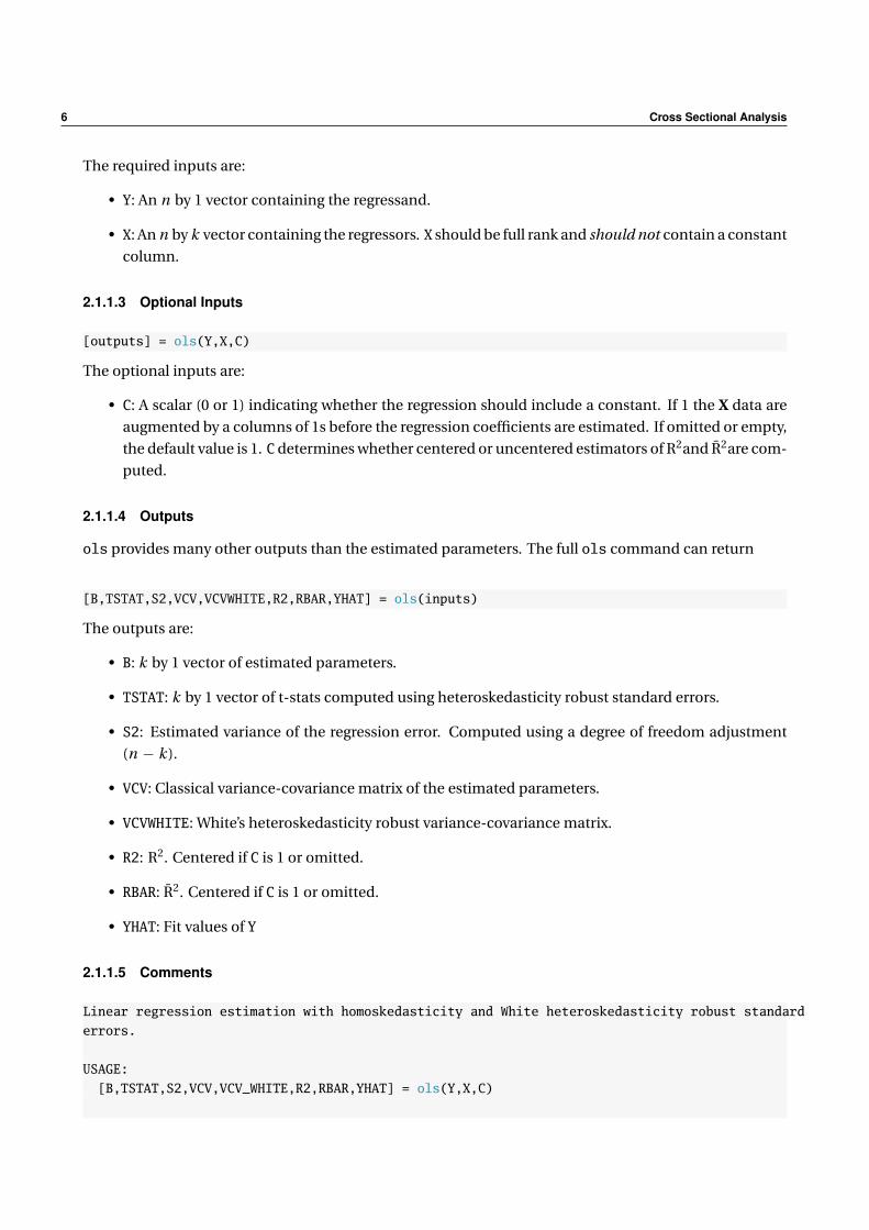
6 Cross Sectional Analysis
The required inputs are:
• Y: An n by 1 vector containing the regressand.
• X: An n by k vector containing the regressors. X should be full rank and should not contain a constant
column.
2.1.1.3 Optional Inputs
[outputs] = ols(Y,X,C)
The optional inputs are:
• C: A scalar (0 or 1) indicating whether the regression should include a constant. If 1 the X data are
augmented by a columns of 1s before the regression coefficients are estimated. If omitted or empty,
the default value is 1. C determines whether centered or uncentered estimators of R2and R2are com-
puted.
2.1.1.4 Outputs
ols provides many other outputs than the estimated parameters. The full ols command can return
[B,TSTAT,S2,VCV,VCVWHITE,R2,RBAR,YHAT] = ols(inputs)
The outputs are:
• B: k by 1 vector of estimated parameters.
• TSTAT: k by 1 vector of t-stats computed using heteroskedasticity robust standard errors.
• S2: Estimated variance of the regression error. Computed using a degree of freedom adjustment
(n − k ).
• VCV: Classical variance-covariance matrix of the estimated parameters.
• VCVWHITE: White’s heteroskedasticity robust variance-covariance matrix.
• R2: R2. Centered if C is 1 or omitted.
• RBAR: R2. Centered if C is 1 or omitted.
• YHAT: Fit values of Y
2.1.1.5 Comments
Linear regression estimation with homoskedasticity and White heteroskedasticity robust standard
errors.
USAGE:
[B,TSTAT,S2,VCV,VCV_WHITE,R2,RBAR,YHAT] = ols(Y,X,C)
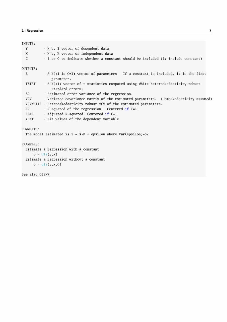
2.1 Regression 7
INPUTS:
Y - N by 1 vector of dependent data
X - N by K vector of independent data
C - 1 or 0 to indicate whether a constant should be included (1: include constant)
OUTPUTS:
B - A K(+1 is C=1) vector of parameters. If a constant is included, it is the first
parameter.
TSTAT - A K(+1) vector of t-statistics computed using White heteroskedasticity robust
standard errors.
S2 - Estimated error variance of the regression.
VCV - Variance covariance matrix of the estimated parameters. (Homoskedasticity assumed)
VCVWHITE - Heteroskedasticity robust VCV of the estimated parameters.
R2 - R-squared of the regression. Centered if C=1.
RBAR - Adjusted R-squared. Centered if C=1.
YHAT - Fit values of the dependent variable
COMMENTS:
The model estimated is Y = X*B + epsilon where Var(epsilon)=S2
EXAMPLES:
Estimate a regression with a constant
b = ols(y,x)
Estimate a regression without a constant
b = ols(y,x,0)
See also OLSNW

8 Cross Sectional Analysis
Chapter 3
Stationary Time Series
3.1 ARMA Simulation
3.1.1 Simulation: armaxfilter_simulate
ARMA and ARMAX simulation using either normal innovations or user-provided residuals.
3.1.1.1 ARMA(P,Q) simulation
An ARMA(P,Q) model is expressed as
yt = φ0 +P∑
p=1
φp yt−p +Q∑
q=1
θqεt−q + εt .
ARMA(P,Q) simulation requires the orders for both the AR and MA portions to be defined. To simulate
an irregular AR(P) - an AR(P) with some coefficients 0 - simply simulate a regular AR(P) and insert 0 for
omitted lags.
3.1.1.2 Examples
The five examples below refer, in order, to
yt = 1 + .9yt−1 + εt (3.1)
yt = 1 + .8εt−1 + εt (3.2)
yt = 1 + 1.5yt−1 − .9yt−2 + .8εt−1 + .4εt−2 + εt (3.3)
yt = 1 + yt−1 − .8yt−3 + εt (3.4)
yt = 1 + .9yt−1 + ηt (3.5)
where εti.i.d.∼ N (0, 1) are standard normally distributed and ηt
i.i.d.∼ t6 are Student’s T with 6 degrees of
freedom distributed.
% Simulates 1000 draws from an AR(1) with phi0 = 1
T=1000; phi = .9; constant = 1; ARorder = 1;
10 Stationary Time Series
y = armaxfilter_simulate(T, constant, ARorder, phi);
% Simulates 1000 draws from an MA(1) with phi0 = 1
theta = .8; MAorder=1; Arorder=0;
y = armaxfilter_simulate(T, constant, 0, [], MAorder, theta);
% Simulates 1000 draws from an ARMA(2,2) with phi0 = 1.
% The parameters are ordered phi = [phi1 phi2] and theta = [theta1 theta2]
theta=[.8 .4]; phi = [1.5 -.9]; MAorder=2; ARorder=2;
y = armaxfilter_simulate(T, constant, ARorder, phi , MAorder, theta);
% Simulates and AR(3) with some coefficients 0 and phi0=0;
constant = 0; phi = [ 1 0 -.8]; ARorder = 3;
y = armaxfilter_simulate(T, constant, ARorder, phi);
% Simulates 1000 draws from an AR(1) with phi0 = 1 using Students-t innovations
e = trnd(6,1000,1);
e=e./sqrt(6/4); % Transforms the errors to have unit variance
T=1000; phi = .9; constant = 1; ARorder = 1;
y = armaxfilter_simulate(e,constant, ARorder, phi);
3.1.1.3 ARMAX(P,Q) simulation
ARMAX simulation extends standard ARMA(P,Q) simulation to include the possibility of exogenous re-
gressors, xk t for k = 1, . . . , K . An ARMAX(P,Q) model is specified
yt = φ0 +P∑
p=1
φp yt−p +K∑
k=1
βk xk ,t−1 +Q∑
q=1
θqεt−q + εt
Note: While the xk ,t−1 terms are all written with a t −1 index, they can be from any time before t by simply
redefining xk ,t−1 to refer to some variable at t − j . For example, x1,t−1 = SP 500t−1, x2,t−1 = SP 500t−2
and so on.
3.1.1.4 Examples
The two examples below refer, in order, to
yt = 1 + .9yt−1 + .5xt−1 + εt (3.6)
yt = 1 + .9yt−1 + .5xt−1 − .2xt−2 + εt (3.7)
where εti.i.d.∼ N (0, 1) are standard normally distributed and xt = .8 ∗ xt−1 + εt .
% First simulate x
T=1001; phi = .8; constant = 0; ARorder = 1; % 1001 needed due to
% losses in lagging
x = armaxfilter_simulate(T, constant, ARorder, phi);
% Then lags x
3.1 ARMA Simulation 11
[x, xlags1] = newlagmatrix(x,1,0);
T=1000; phi = .9; constant = 1; ARorder = 1; Xp=.5; X=xlags1;
y = armaxfilter_simulate(T, constant, ARorder, phi, 0, [], X, Xp);
% First simulate x
T=1002; phi = .8; constant = 0; ARorder = 1; % 1002 needed due to
% losses in lagging
x = armaxfilter_simulate(T, constant, ARorder, phi);
% Then lags x
[x, xlags12] = newlagmatrix(x,2,0);
T=1000; phi = .9; constant = 1; ARorder = 1; Xp=[.5 -.2]; X=xlags12;
y = armaxfilter_simulate(T, constant, ARorder, phi, 0, [], X, Xp);
3.1.1.5 Required Inputs
[outputs] = armaxfilter_simulate(T,CONST)
• T: Either a scalar integer or a vector of random numbers. If scalar, T represents the length of the
time series to simulate. If a T by 1 vector of random numbers, these will be used to construct the
simulated time series.
• CONST: Scalar value containing the constant term in the simulated model
3.1.1.6 Optional Inputs
[outputs] = armaxfilter_simulate(T,CONST,AR,ARPARAMS,MA,MAPARAMS,X,XPARAMS)
• AR: Order of AR in simulated model
• ARPARAMS: Column vector containing AR elements containing the values of the parameters on the
AR terms. Ordered from smallest to largest.
• MA: Order of MA in simulated model
• MAPARAMS: Column vector containing MA elements containing the values of the parameters on the
MA terms. Ordered from smallest to largest.
• X: T by k matrix of exogenous variables
• XPARAMS: k by 1 vector of parameters for the exogenous variables.
3.1.1.7 Outputs
[Y,ERRORS] = armaxfilter_simulate(inputs)
• Y: T by 1 vector of simulated data
• ERRORS: T by 1 vector of errors used to construct the simulated data
12 Stationary Time Series
3.1.1.8 Comments
ARMAX(P,Q) simulation with normal errors. Also simulates AR, MA and ARMA models.
USAGE:
AR:
[Y,ERRORS]=armaxfilter_simulate(T,CONST,AR,ARPARAMS)
MA:
[Y,ERRORS]=armaxfilter_simulate(T,CONST,0,[],MA,MAPARAMS)
ARMA:
[Y,ERRORS]=armaxfilter_simulate(T,CONST,AR,ARPARAMS,MA,MAPARAMS);
ARMAX:
[Y,ERRORS]=armaxfilter_simulate(T,CONST,AR,ARPARAMS,MA,MAPARAMS,X,XPARAMS);
INPUTS:
T - Length of data series to be simulated OR
T by 1 vector of user supplied random numbers (e.g. rand(1000,1)-0.5)
CONST - Value of the constant in the model. To omit, set to 0.
AR - Order of AR in model. To include only selected lags, for example t-1 and t-3, use 3
and set the coefficient on 2 to 0
ARPARAMS - AR by 1 vector of parameters for the AR portion of the model
MA - Order of MA in model. To include only selected lags of the error, for example t-1
and t-3, use 3 and set the coefficient on 2 to 0
MAPARAMS - MA by 1 vector of parameters for the MA portion of the model
X - T by K matrix of exogenous variables
XPARAMS - K by 1 vector of parameters on the exogenous variables
OUTPUTS:
Y - A T by 1 vector of simulated data
ERRORS - The errors used in the simulation
COMMENTS:
The ARMAX(P,Q) model simulated is:
y(t) = const + arp(1)*y(t-1) + arp(2)*y(t-2) + ... + arp(P) y(t-P) +
+ ma(1)*e(t-1) + ma(2)*e(t-2) + ... + ma(Q) e(t-Q)
+ xp(1)*x(t,1) + xp(2)*x(t,2) + ... + xp(K)x(t,K)
+ e(t)
EXAMPLES:
Simulate an AR(1) with a constant
y = armaxfilter_simulate(500, .5, 1, .9)
Simulate an AR(1) without a constant
y = armaxfilter_simulate(500, 0, 1, .9)
Simulate an ARMA(1,1) with a constant
y = armaxfilter_simulate(500, .5, 1, .95, 1, -.5)
Simulate a MA(1) with a constant
y = armaxfilter_simulate(500, .5, [], [], 1, -.5)
Simulate a seasonal MA(4) with a constant
y = armaxfilter_simulate(500, .5, [], [], 4, [.6 0 0 .2])
See also ARMAXFILTER, HETEROGENEOUSAR
3.2 ARMA Estimation 13
3.2 ARMA Estimation
3.2.1 Estimation: armaxfilter
Provides ARMA and ARMAX estimation for time-series models.
3.2.1.1 AR(1) and AR(P)
As special cases of an ARMAX, AR(1) and AR(P), both regular and irregular, can be estimated using
armaxfilter. The AR(1),
yt = φ0 + φ1 yt−1 + εt
can be estimated using
parameters = armaxfilter(y,1,1)
where the first argument is the time series, the second argument takes the value 1 or 0 to indicate whether a
constant should be included in the model (i.e. if it were 0, the model yt = φ1 yt−1+εt would be estimated),
and the third argument contains the autoregressive lags to be included in the model. An AR(P),
yt = φ0 + φ1 yt−1 + . . . + φP yt−P + εt
can be similarly estimated
P = 3;
parameters = armaxfilter(y,1,[1:P])
which would estimate an AR(3). The final argument in armaxfilter is [1:3] because all three lags of y ,
yt−1, yt−2 and yt−3 should be included (Note that [1:3] = [1 2 3]). An irregular AR(3) that includes
only the first and third lag, yt = φ0 + φ1 yt−1 + φ3 yt−3 + εt can be fit using
parameters = armaxfilter(y,1,[1 3])
where the final argument changes from [1:3] to [1 3] to indicate that only lags 1 and 3 should be in-
cluded.
3.2.1.2 MA(1) and MA(P)
Estimation of MA(1) and MA(Q) models is similar to estimation of AR(P) models. The commands to the
MA coefficient in armaxfilter are identical and the AR coefficients are set to 0 (or empty, []). Estimation
of an MA(1),
yt = θ1εt−1 + εt
can be accomplished by calling
parameters = armaxfilter(y,1,[],1)
14 Stationary Time Series
where the empty argument ([]) indicates that no AR terms are to be included. Parameter estimates for an
MA(Q),
yt = φ0 + θ1εt−1 + . . . + θQεt−Q + εt
can be computed by calling
Q=3;
parameters = armaxfilter(y,1,[],[1:Q])
and an irregular MA(3) that only includes lags 1 and 3 can be estimated by replacing the final argument,
[1:3], with [1 3].
parameters = armaxfilter(y,1,[],[1 3])
3.2.1.3 ARMA(P,Q)
Regular and Irregular ARMA(P,Q) estimation simply combines the two above steps. For example, to esti-
mate a regular ARMA(1,1),
yt = φ0 + φ1 yt−1 + θ1εt−1 + εt
call
parameters = armaxfilter(y,1,1,1)
Estimation of regular ARMA(P,Q) is straightforward.
yt = φ0 + φ1 yt−1 + . . . + φP yt−P + θ1εt−1 + . . . + θQεt−Q + εt
is estimated using the command
P=3; Q=4;
parameters = armaxfilter(y,1,1:P,1:Q)
and irregular ARMA(P,Q) processes can be computed by replacing the regular arrays [1:P] and [1:Q]with
arrays of only the lags to be included,
parameters = armaxfilter(y,1,[1 3],[1 4])
3.2.1.4 ARX(P), MAX(Q) and ARMAX(P,Q)
Including exogenous variables in AR(P), MA(Q) and ARMA(P,Q) models is identical to the above save one
additional step needed to align the data. Suppose that two time series yt and xt are available and
that they are aligned, so that x1 and y1 are from the same point in time. To regress yt on one lag of itself
and a lag of xt , it is necessary to promote x so that the element in the sth position is actually xs−1 and thus
3.2 ARMA Estimation 15
that yt will be coupled with xt−1. This is simple to do using the command newlagmatrix. newlagmatrix
produces two outputs, a vector of contemporary values that has been adjusted to remove lags (i.e. if the
original series has T observations, and newlagmatrix is requested to produce 2 lags, the new series will
have T − 2.) and a matrix of lags of the form yt−1 yt−2 . . . yt−P . To estimate an ARX(P), it is necessary to
adjust both x and y so that they line up. For example, to estimate
yt = φ0 + φ1 yt−1 + β1 xt−1 + εt ,
call
[yadj, ylags] = newlagmatrix(y,1,0);
[xadj, xlags] = newlagmatrix(x,1,0);
% Regress the adjusted values of y on the lags of x
X = xlags;
parameters = armaxfilter(yadj,1,1,0,X);
Aside from the step needed to properly align the data, estimating ARX(P), MAX(Q) and ARMAX(P,Q) mod-
els is identical to AR(P), MA(Q) and ARMA(P,Q). Regular models can be estimated by including 1:P or 1:Q
and irregular models can be estimated using irregular arrays (e.g. [1 3] or [1 2 4]).
The key to estimating ARMAX(P,Q) models is to lags both y and x by as many lags of x as are included
in the model. Consider the final example of an ARMAX(1,1) where 3 lags of x are to be included,
yt = φ0 + φ1 yt−1 + β1 xt−1 + β2 xt−2 + β3 xt−3 + θ1εt−1 + εt .
Assuming that the original x and y data “line-up” - so that x(1) and y(1) occurred at the same point in
time - this model can be estimated using the following code:
[yadj, ylags] = newlagmatrix(y,3,0);
[xadj, xlags] = newlagmatrix(x,3,0);
% Regress the adjusted values of y on the lags of x
X = xlags;
parameters = armaxfilter(yadj,1,1,1,X);
3.2.1.5 Required Inputs
[outputs] = armaxfilter(Y,CONSTANT)
The required inputs are:
• Y: T by 1 vector containing the dependant variable.
• CONSTANT: Logical value indicating whether to include a constant (1 to include, 0 to exclude).
Note: The required inputs only estimate the (unconditional) mean, and so it will generally be necessary
to use some of the optional inputs.
16 Stationary Time Series
3.2.1.6 Optional Inputs
[outputs] = armaxfilter(Y,CONSTANT,P,Q,X,STARTINGVALS,OPTIONS,HOLDBACK)
The optional inputs are:
• P: Column vector containing indices for the AR component in the model.
• Q: Column vector containing indices for the MA component in the model
• X: T by k matrix of exogenous regressors. Should be aligned with Y so that the ith row of X is known
when the observation in the ith row of Y is observed.
• STARTINGVALS: Column vector containing starting values for estimation. Used only for models with
an MA component.
• OPTIONS: MATLAB options structure for optimization using lsqnonlin.
• HOLDBACK: Scalar integer indicating the number of observations to withhold at the start of the sam-
ple. Useful when testing models with different lag lengths to produce comparable likelihoods, AICs
and SBICs. Should be set to the highest lag length (AR or MA) in the models studied.
3.2.1.7 Outputs
armaxfilter provides many other outputs than the estimated parameters. The full armaxfilter com-
mand can return
[PARAMETERS, LL, ERRORS, SEREGRESSION, DIAGNOSTICS, VCVROBUST, VCV, LIKELIHOODS, SCORES]
=armaxfilter(inputs here)
The outputs are:
• PARAMETERS: A vector of estimated parameters. The size of parameters is determined by whether
the constant is included, the number of lags included in the AR and MA portions and the number
of exogenous variables included (if any).
• LL: The log-likelihood computed using the estimated residuals and assuming a normal distribution.
• ERRORS: A T by 1 vector of estimated errors from the model
• SEREGRESSION: Standard error of the regression. Estimated using a degree-of-freedom adjustment.
• DIAGNOSTICS: A MATLAB structure of output that may be useful. To access elements of a structure,
enter diagnostics.fieldname where fieldname is one of:
– P: The AR lags used in estimation
– Q: The MA lags used in estimation
– C: An indicator (1 or 0) indicating whether a constant was included.
– NX: The number of X variables in the regression
3.2 ARMA Estimation 17
– AIC: The Akaike Information Criteria (AIC) for the estimated model
– SBIC: The Schwartz/Bayesian Information Criteria (SBIC) for the estimated model
– T: The number of observations in the original data series
– ADJT: The number of observations used for estimation after adjusting for HOLDBACK or requires
AR lag adjustments.
– ARROOTS: The characteristic roots of the characteristic equation corresponding to the estimated
ARMA model.
– ABSARROOTS: The absolute value of the arroots
• VCVROBUST: Heteroskedasticity-robust covariance matrix for the estimated parameters. The square-
root of the ith diagonal element is the standard deviation of the ith element of PARAMETERS.
• VCV: Non-heteroskedasticity robust covariance matrix of the estimated parameters.
• LIKELIHOODS: A T by 1 vector of the log-likelihood of each observation.
• SCORES: A T by # parameters matrix of scores of the model. These are used in some advanced test.
3.2.1.8 Examples
See above.
3.2.1.9 Comments
ARMAX(P,Q) estimation
USAGE:
[PARAMETERS]=armaxfilter(Y,CONSTANT,P,Q)
[PARAMETERS, LL, ERRORS, SEREGRESSION, DIAGNOSTICS, VCVROBUST, VCV, LIKELIHOODS, SCORES]
=armaxfilter(Y,CONSTANT,P,Q,X,STARTINGVALS,OPTIONS,HOLDBACK)
INPUTS:
Y - A column of data
CONSTANT - Scalar variable: 1 to include a constant, 0 to exclude
P - Non-negative integer vector representing the AR orders to include in the model.
Q - Non-negative integer vector representing the MA orders to include in the model.
X - [OPTIONAL] a T by K matrix of exogenous variables. These line up exactly with
the Y’s and if they are time series, you need to shift them down by 1 place,
i.e. pad the bottom with 1 observation and cut off the top row [ T by K].
For
example, if you want to include X(t-1) as a regressor, Y(t) should line up
with X(t-1)
STARTINGVALS - [OPTIONAL] A (CONSTANT+length(P)+length(Q)+K) vector of starting values.
[constant ar(1) ... ar(P) xp(1) ... xp(K) ma(1) ... ma(Q) ]’
OPTIONS - [OPTIONAL] A user provided options structure. Default options are below.
HOLDBACK - [OPTIONAL] Scalar integer indicating the number of observations to withhold at
the start of the sample. Useful when testing models with different lag lengths
18 Stationary Time Series
to produce comparable likelihoods, AICs and SBICs. Should be set to the highest
lag length (AR or MA) in the models studied.
OUTPUTS:
PARAMETERS - A 1+length(p)+size(X,2)+length(q) column vector of parameters with
[constant ar(1) ... ar(P) xp(1) ... xp(K) ma(1) ... ma(Q) ]’
LL - The log-likelihood of the regression
ERRORS - A T by 1 length vector of errors from the regression
SEREGRESSION - The standard error of the regressions
DIAGNOSTICS - A structure of diagnostic information containing:
P - The AR lags used in estimation
Q - The MA lags used in estimation
C - Indicator if constant was included
nX - Number of X variables in the regression
AIC - Akaike Information Criteria for the estimated model
SBIC - Bayesian (Schwartz) Information Criteria for the
estimated model
ADJT - Length of sample used for estimation after HOLDBACK adjustments
T - Number of observations
ARROOTS - The characteristic roots of the ARMA
process evaluated at the estimated parameters
ABSARROOTS - The absolute value (complex modulus if
complex) of the ARROOTS
VCVROBUST - Robust parameter covariance matrix%
VCV - Non-robust standard errors (inverse Hessian)
LIKELIHOODS - A T by 1 vector of log-likelihoods
SCORES - Matrix of scores (# of params by T)
COMMENTS:
The ARMAX(P,Q) model is:
y(t) = const + arp(1)*y(t-1) + arp(2)*y(t-2) + ... + arp(P) y(t-P) +
+ ma(1)*e(t-1) + ma(2)*e(t-2) + ... + ma(Q) e(t-Q)
+ xp(1)*x(t,1) + xp(2)*x(t,2) + ... + xp(K)x(t,K)
+ e(t)
The main optimization is performed with lsqnonlin with the default options:
options = optimset(’lsqnonlin’);
options.MaxIter = 10*(maxp+maxq+constant+K);
options.Display=’iter’;
You should use the MEX file (or compile if not using Win64 Matlab) for armaxerrors.c as it
provides speed ups of approx 10 times relative to the m file version armaxerrors.m
EXAMPLE:
To fit a standard ARMA(1,1), use
parameters = armaxfilter(y,1,1,1)
To fit a standard ARMA(3,4), use
parameters = armaxfilter(y,1,[1:3],[1:4])
To fit an ARMA that includes lags 1 and 3 of y and 1 and 4 of the MA term, use

3.2 ARMA Estimation 19
parameters = armaxfilter(y,1,[1 3],[1 4])
See also ARMAXFILTER_SIMULATE, HETEROGENEOUSAR, ARMAXERRORS
20 Stationary Time Series
3.2.2 Heterogeneous Autoregression: heterogeneousar
Estimates heterogeneous autoregressions, which are restricted parameterizations of standard ARs. A HAR
is a model of the class
yt = φ0 +P∑
i=1
φi yt−1:i + εt
where yt−1:i = i−1∑ij=1 yt− j . If all lags are included from 1 to P then the HAR is just a re-parameterized
Pth order AR, and so it is generally the case that most lags are set to zero, as in the common volatility HAR,
yt = φ0 + φ1 yt−1 + φ5 yt−1:5 + φ22 yt−1:22 + εt
where yt−1:1 = yt−1.
3.2.2.1 Examples
% Simulate data from a HAR model
y = armaxfilter_simulate(1000,1,22,[.1 .3/4*ones(1,4) .55/17*ones(1,17)])
% Standard HAR with 1, 5 and 22 day lags
parameters = heterogeneousar(Y,1,[1 5 22]’)
% Standard HAR with 1, 5 and 22 days lags using matrix notation
parameters = heterogeneousar(Y,1,[1 1;1 5;1 22])
% Standard HAR with 1, 5 and 22 day lags using the non-overlapping reparameterization
parameters = heterogeneousar(Y,1,[1 5 22]’,[],’MODIFIED’)
% Standard HAR with 1, 5 and 22 day lags with Newey-West standard errors
[parameters, errors, seregression, diagnostics, vcvrobust, vcv] = ...
heterogeneousar(Y,1,[1 5 22]’,ceil(length(Y)^(1/3)))
% Nonstandard HAR with lags 1, 2 and 10-22 day lags
parameters = heterogeneousar(Y,1,[1 1;2 2;10 22])
3.2.2.2 Required Inputs
[outputs] = heterogeneousar(Y,CONSTANT,P)
The required inputs are:
• Y: T by 1 vector containing the dependant variable.
• CONSTANT: Logical value indicating whether to include a constant (1 to include, 0 to exclude).
• P: Vector or Matrix. If a vector, must be a column vector. The values are interpreted as the number
of lags to average in each term. For example, [1 5 22] would fit the HAR
yt = φ0 + φ1 yt−1 + φ5 yt−1:5 + φ22 yt−1:22 + εt .
If a matrix, must be number of terms by 2 where the first column indicates the start point and the
3.2 ARMA Estimation 21
second indicates the end point. The matrix equivalent to the above vector notation is 1 1
1 5
1 22
.
The matrix notation allows a HAR with non-overlapping intervals to be specified, such as 1 1
2 5
10 22
which would fit the model
yt = φ0 + φ1 yt−1 + φ5 yt−2:5 + φ22 yt−10:22 + εt .
3.2.2.3 Optional Inputs
[outputs] = heterogeneousar(Y,CONSTANT,P,NW,SPEC)
The optional inputs are:
• NW: Number of lags to include when computing the covariance of the estimated parameters. Default
is 0.
• SPEC: String value, either ’STANDARD’ or ’MODIFIED’. Modified reparameterizes the usual HAR as a
series of non-overlapping intervals, and so
yt = φ0 + φ1 yt−1 + φ5 yt−1:5 + φ22 yt−1:22 + εt
would be reparameterized as
yt = φ0 + φ1 yt−1 + φ5 yt−2:5 + φ22 yt−6:22 + εt
when estimated. The model fits are identical, and the ’MODIFIED’ version is only helpful for presen-
tation and interpretation.
3.2.2.4 Outputs
[PARAMETERS, ERRORS, SEREGRESSION, DIAGNOSTICS, VCVROBUST, VCV] = heterogeneousar(inputs)
• PARAMETERS: A vector of estimated parameters. The size of parameters is determined by whether
the constant is included and the number of lags included in the HAR.
• ERRORS: A T by 1 vector of estimated errors from the model. The first max(max(P)) are set to 0.
• SEREGRESSION: Standard error of the regression. Estimated using a degree-of-freedom adjustment.
• DIAGNOSTICS: A MATLAB structure of output that may be useful. To access elements of a structure,
enter diagnostics.fieldname where fieldname is one of:
22 Stationary Time Series
– P: The AR lags used in estimation
– C: An indicator (1 or 0) indicating whether a constant was included.
– AIC: The Akaike Information Criteria (AIC) for the estimated model
– SBIC: The Schwartz/Bayesian Information Criteria (SBIC) for the estimated model
– T: The number of observations in the original data series
– ADJT: The number of observations used for estimation after adjusting for AR lag length.
– ARROOTS: The characteristic roots of the characteristic equation corresponding to the estimated
ARMA model.
– ABSARROOTS: The absolute value of the arroots
• VCVROBUST: Heteroskedasticity-robust covariance matrix for the estimated parameters. Also auto-
correlation robust if NW selected appropriately. The square-root of the ith diagonal element is the
standard deviation of the ith element of PARAMETERS.
• VCV: Non-heteroskedasticity robust covariance matrix of the estimated parameters.
3.2.2.5 Comments
Heterogeneous Autoregression parameter estimation
USAGE:
[PARAMETERS] = heterogeneousar(Y,CONSTANT,P)
[PARAMETERS, ERRORS, SEREGRESSION, DIAGNOSTICS, VCVROBUST, VCV]
= heterogeneousar(Y,CONSTANT,P,NW,SPEC)
INPUTS:
Y - A column of data
CONSTANT - Scalar variable: 1 to include a constant, 0 to exclude
P - A column vector or a matrix.
If a vector, should include the indices to use for the lag length, such as in
the usual case for monthly volatility data P=[1; 5; 22]. This indicates that
the 1st lag, average of the first 5 lags, and the average of the first 22 lags
should be used in estimation. NOTE: When using the vector format, P MUST BE A
COLUMN VECTOR to avoid ambiguity with the matrix format. If P is a matrix, the
values indicate the start and end points of the averages. The above vector can
be equivalently expressed as P=[1 1;1 5;1 22]. The matrix notation allows for
the possibility of skipping lags, for example P=[1 1; 5 5; 1 22]; would have
the 1st lag, the 5th lag and the average of lags 1 to 22. NOTE: When using the
matrix format, P MUST be # Entries by 2.
NW - [OPTIONAL] Number of lags to use when computing the long-run variance of the
scores in VCVROBUST. Default is 0.
SPEC - [OPTIONAL] String value indicating which representation to use in parameter
estimation. May be:
’STANDARD’ - Usual representation with overlapping lags
’MODIFIED’ - Modified representation with non-overlapping lags
3.2 ARMA Estimation 23
OUTPUTS:
PARAMETERS - A 1+length(p) column vector of parameters with
[constant har(1) ... har(P)]’
ERRORS - A T by 1 length vector of errors from the regression with 0s in first max(max(P))
places
SEREGRESSION - The standard error of the regressions
DIAGNOSTICS - A structure of diagnostic information containing:
P - List of HAR lags used in estimation
C - Indicator if constant was included
AIC - Akaike Information Criteria for the estimated model
SBIC - Bayesian (Schwartz) Information Criteria for the
estimated model
T - Number of observations
ADJT - Length of sample used for estimation
ARROOTS - The characteristic roots of the ARMA
process evaluated at the estimated parameters
ABSARROOTS - The absolute value (complex modulus if
complex) of the ARROOTS
VCVROBUST - Robust parameter covariance matrix, White if NW = 0,
Newey-West if NW>0
VCV - Non-robust standard errors (inverse Hessian)
EXAMPLES:
Simulate data from a HAR model
y = armaxfilter_simulate(1000,1,22,[.1 .3/4*ones(1,4) .55/17*ones(1,17)])
Standard HAR with 1, 5 and 22 day lags
parameters = heterogeneousar(Y,1,[1 5 22]’)
Standard HAR with 1, 5 and 22 days lags using matrix notation
parameters = heterogeneousar(Y,1,[1 1;1 5;1 22])
Standard HAR with 1, 5 and 22 day lags using the non-overlapping reparameterization
parameters = heterogeneousar(Y,1,[1 5 22]’,[],’MODIFIED’)
Standard HAR with 1, 5 and 22 day lags with Newey-West standard errors
[parameters, errors, seregression, diagnostics, vcvrobust, vcv] = ...
heterogeneousar(Y,1,[1 5 22]’,ceil(length(Y)^(1/3)))
Nonstandard HAR with lags 1, 2 and 10-22 day lags
parameters = heterogeneousar(Y,1,[1 1;2 2;10 22])
See also ARMAXFILTER, TARCH
24 Stationary Time Series
3.2.3 Residual Plotting: tsresidualplot
Provides a convenient tool to quickly plot errors from ARMA models.
3.2.3.1 Examples
T=1000; phi = .9; constant = 1; ARorder = 1;
y = armaxfilter_simulate(T, constant, ARorder, phi);
% ARMA(1,1) with a constant;
[parameters, LL, errors] = armaxfilter(y, 1, 1, 1);
tsresidualplot(y,errors)
% With dates for 1000 days beginning at Jan 1 2007
dates = datenum(’Jan-01-2007’):datenum(’Jan-01-2007’)+999;
% ARMA(1,1) with a constant;
[parameters, LL, errors] = armaxfilter(y, 1, 1, 1);
tsresidualplot(y,errors, dates)
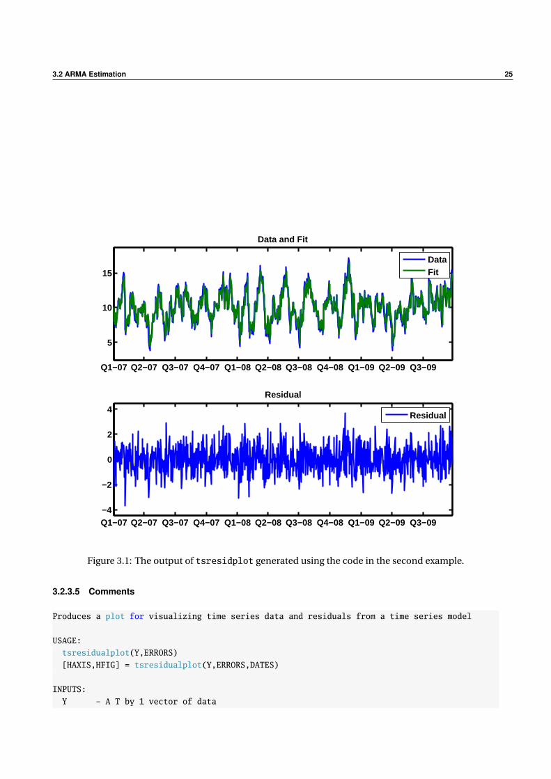
The output of tsresidualplot is in figure 3.1 (this was generated suing the second command above):
3.2.3.2 Required Inputs
[outputs] = tsresidualplot(Y,ERRORS)
• Y: T by 1 vector of modeled data
• ERRORS: T by 1 vector of residuals
3.2.3.3 Optional Inputs
[outputs] = tsresidualplot(Y,ERRORS,DATES)
• DATES: T by 1 vector of MATLAB serial dates
3.2.3.4 Outputs
[HAXIS,HFIG] = tsresidualplot(inputs)
• HAXIS: 2 by 1 vector of handles to the plot axes
• HFIG: Handle to the figure containing the residual plot
3.2 ARMA Estimation 25
Q1−07 Q2−07 Q3−07 Q4−07 Q1−08 Q2−08 Q3−08 Q4−08 Q1−09 Q2−09 Q3−09
5
10
15
Data and Fit
DataFit
Q1−07 Q2−07 Q3−07 Q4−07 Q1−08 Q2−08 Q3−08 Q4−08 Q1−09 Q2−09 Q3−09−4
−2
0
2
4
Residual
Residual
Figure 3.1: The output of tsresidplot generated using the code in the second example.
3.2.3.5 Comments
Produces a plot for visualizing time series data and residuals from a time series model
USAGE:
tsresidualplot(Y,ERRORS)
[HAXIS,HFIG] = tsresidualplot(Y,ERRORS,DATES)
INPUTS:
Y - A T by 1 vector of data
26 Stationary Time Series
ERRORS - A T by 1 vector of residuals, usually produced by ARMAXFILTER
DATES - [OPTIONAL] A T by 1 vector of MATLAB dates (i.e. should be 733043 rather than ’1-1-2007’).
If provided, the data and residuals will be plotted against the date rather than the
observation index
OUTPUTS:
HAXIS - A 2 by 1 vector axis handles to the top subplots
HFIG - A scalar containing the figure handle
COMMENTS:
HAXIS can be used to change the format of the dates on the x-axis when MATLAB dates are provides
by calling
datetick(HAXIS(j),’x’,DATEFORMAT,’keeplimits’)
where j is 1 (top) or 2 (bottom subplot) and DATEFORMAT is a numeric value between 28. See doc
datetick for more details. For example,
datetick(HAXIS(1),’x’,25,’keeplimits’)
will change the top subplot’s x-axis labels to the form yy/mm/dd.
EXAMPLES:
Estimate a model and produce a plot of fitted and residuals
[parameters, LL, errors] = armaxfilter(y, 1, 1, 1);
tsresidualplot(y, errors)
Estimate a model and produce a plot of fitted and residuals with dates
[parameters, LL, errors] = armaxfilter(y, 1, 1, 1);
dates = datenum(’01Jan2007’) + (1:length(y));
tsresidualplot(y, errors, dates)
See also ARMAXFILTER, DATETICK
3.2 ARMA Estimation 27
3.2.4 Characteristic Roots: armaroots
Computes the characteristic roots (and their absolute values) of the characteristic equation that corre-
spond to an ARMAX(P,Q) equation. It is usually called after or during armaxfilter.
3.2.4.1 Examples
armaroots can be used with either the output of armaxfilter or with hypothetical parameters. The first
example shows how to use them with armaxfilter while the second and third demonstrate their use
with hypothetical ARMA parameters. Note that the AR and MA lag lengths are identical to those used in
armaxfilter, so a regular ARMA(P,Q) requires [1:P] and [1:Q] to be input. This allows roots of irregular
ARMA(P,Q) to be computed by including the indices of the lags used (i.e. [1 3]).
T=1000; phi = .9; constant = 1; ARorder = 1;
y = armaxfilter_simulate(T, constant, ARorder, phi);
% ARMA(1,1) with a constant;
[parameters, LL, errors] = armaxfilter(y, 1, 1, 1);
[arroots, absarroots] = armaroots(parameters, 1, 1, 1)
arroots =
0.9023
absarroots =
0.9023
% An ARMA(2,2)
phi = [1.3 -.35]; theta = [.4 .3]; parameters=[1 phi theta]’;
[arroots, absarroots] = armaroots(parameters, 1, [1 2], [1 2])
arroots =
0.9193
0.3807
absarroots =
0.9193
0.3807
% An irregular AR(3)
% Note that phi contains phi1 and phi3 and that there is no phi2
phi = [1.3 -.35]; parameters = [1 phi]’;
% There will be three roots
[arroots, absarroots] = armaroots(parameters, 1, [1 3],[])
arroots =
0.8738 + 0.1364i
0.8738 - 0.1364i
-0.4475
absarroots =
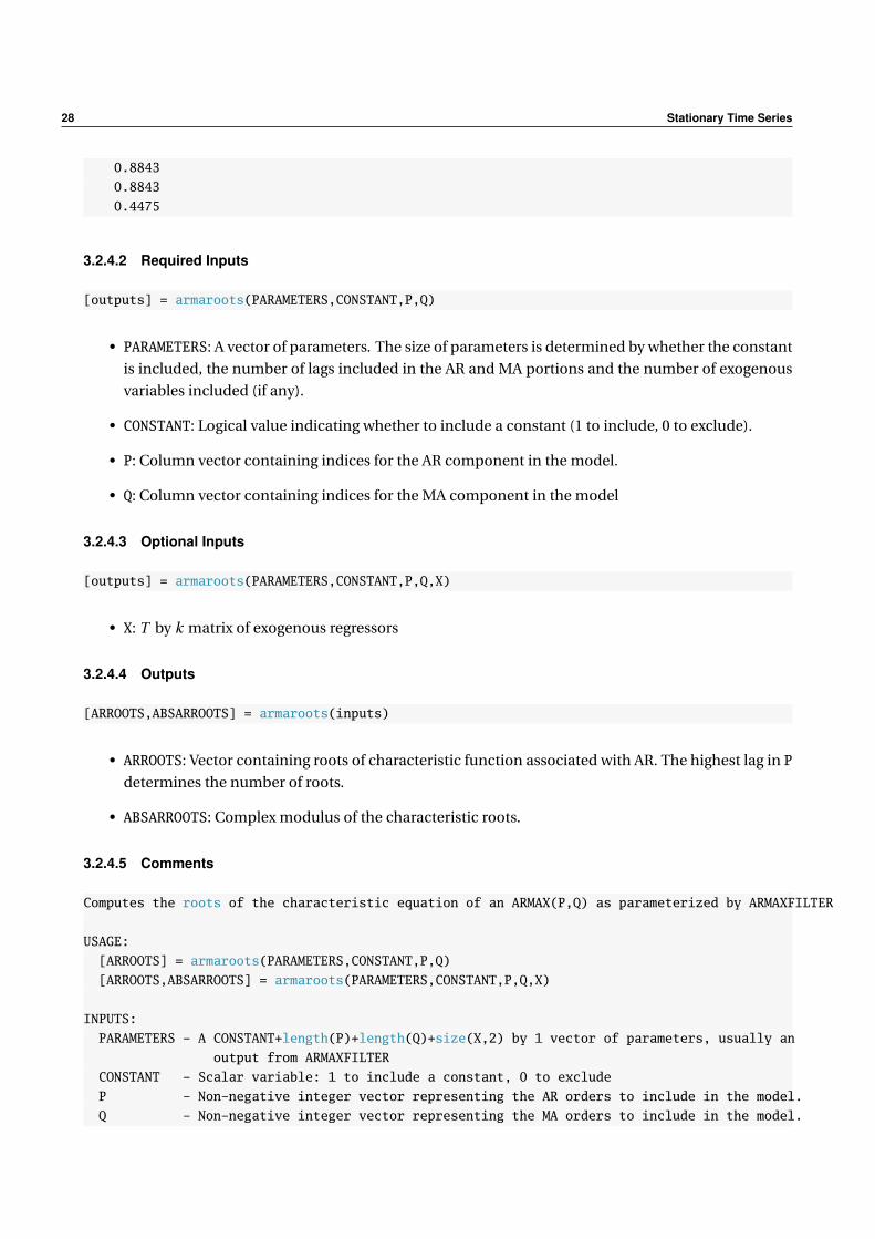
28 Stationary Time Series
0.8843
0.8843
0.4475
3.2.4.2 Required Inputs
[outputs] = armaroots(PARAMETERS,CONSTANT,P,Q)
• PARAMETERS: A vector of parameters. The size of parameters is determined by whether the constant
is included, the number of lags included in the AR and MA portions and the number of exogenous
variables included (if any).
• CONSTANT: Logical value indicating whether to include a constant (1 to include, 0 to exclude).
• P: Column vector containing indices for the AR component in the model.
• Q: Column vector containing indices for the MA component in the model
3.2.4.3 Optional Inputs
[outputs] = armaroots(PARAMETERS,CONSTANT,P,Q,X)
• X: T by k matrix of exogenous regressors
3.2.4.4 Outputs
[ARROOTS,ABSARROOTS] = armaroots(inputs)
• ARROOTS: Vector containing roots of characteristic function associated with AR. The highest lag in P
determines the number of roots.
• ABSARROOTS: Complex modulus of the characteristic roots.
3.2.4.5 Comments
Computes the roots of the characteristic equation of an ARMAX(P,Q) as parameterized by ARMAXFILTER
USAGE:
[ARROOTS] = armaroots(PARAMETERS,CONSTANT,P,Q)
[ARROOTS,ABSARROOTS] = armaroots(PARAMETERS,CONSTANT,P,Q,X)
INPUTS:
PARAMETERS - A CONSTANT+length(P)+length(Q)+size(X,2) by 1 vector of parameters, usually an
output from ARMAXFILTER
CONSTANT - Scalar variable: 1 to include a constant, 0 to exclude
P - Non-negative integer vector representing the AR orders to include in the model.
Q - Non-negative integer vector representing the MA orders to include in the model.
3.2 ARMA Estimation 29
X - [OPTIONAL] A T by K matrix of exogenous variables.
OUTPUTS:
ARROOTS - A max(P) by 1 vector containing the roots of the characteristic equation
corresponding to the ARMA model input
ABSARROOTS - Absolute value or complex modulus of the autoregressive roots
COMMENTS:
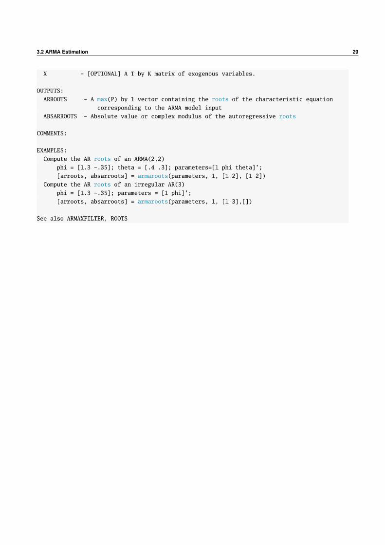
EXAMPLES:
Compute the AR roots of an ARMA(2,2)
phi = [1.3 -.35]; theta = [.4 .3]; parameters=[1 phi theta]’;
[arroots, absarroots] = armaroots(parameters, 1, [1 2], [1 2])
Compute the AR roots of an irregular AR(3)
phi = [1.3 -.35]; parameters = [1 phi]’;
[arroots, absarroots] = armaroots(parameters, 1, [1 3],[])
See also ARMAXFILTER, ROOTS
30 Stationary Time Series
3.2.5 Information Criteria: aicsbic
Computes the Akaike Information Criteria (AIC) and the Schwartz/Bayes Information Criterion for an
ARMAX(P,Q). The AIC is given by
AI C = ln σ2 +2k
T
where k is the number of parameters in the model, including the constant, AR coefficients, MA coefficient
and any X variables. The SBIC is given by
S B I C = ln σ2 +ln T k
T.
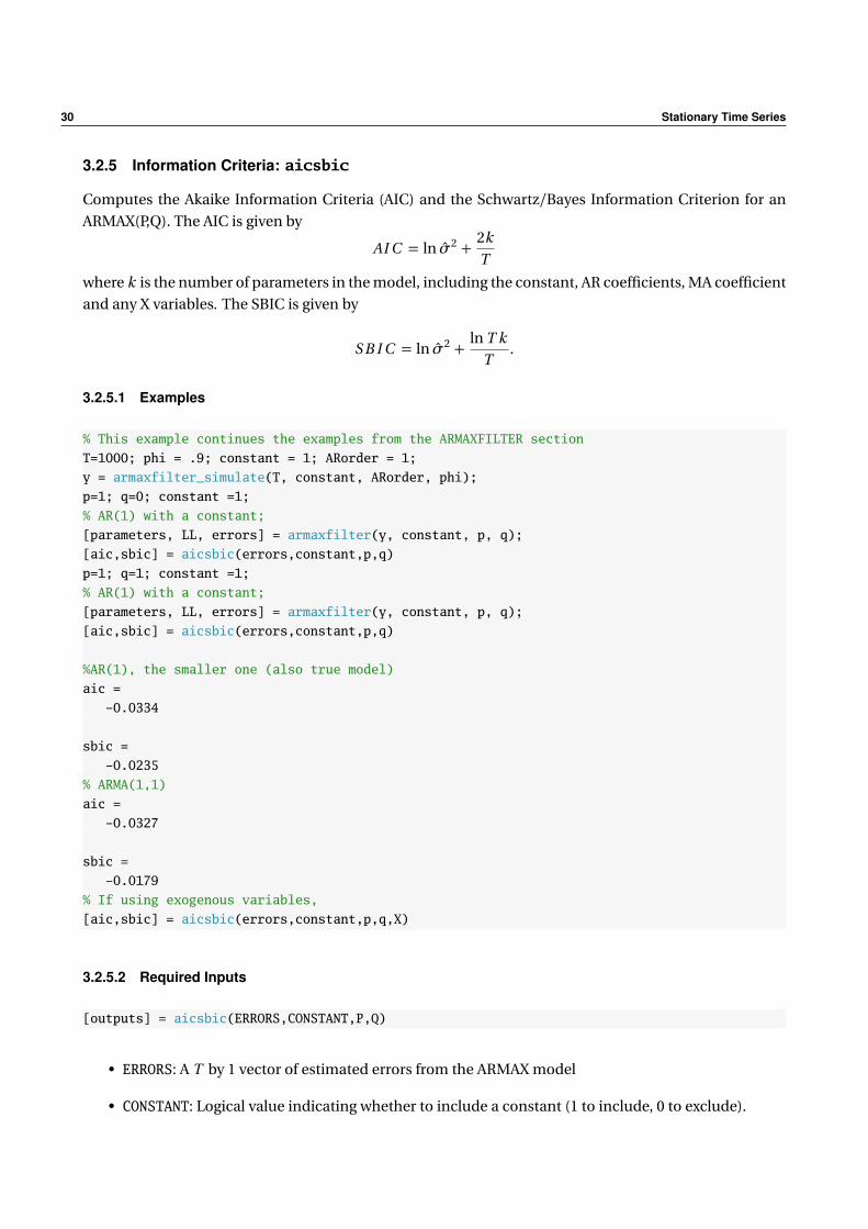
3.2.5.1 Examples
% This example continues the examples from the ARMAXFILTER section
T=1000; phi = .9; constant = 1; ARorder = 1;
y = armaxfilter_simulate(T, constant, ARorder, phi);
p=1; q=0; constant =1;
% AR(1) with a constant;
[parameters, LL, errors] = armaxfilter(y, constant, p, q);
[aic,sbic] = aicsbic(errors,constant,p,q)
p=1; q=1; constant =1;
% AR(1) with a constant;
[parameters, LL, errors] = armaxfilter(y, constant, p, q);
[aic,sbic] = aicsbic(errors,constant,p,q)
%AR(1), the smaller one (also true model)
aic =
-0.0334
sbic =
-0.0235
% ARMA(1,1)
aic =
-0.0327
sbic =
-0.0179
% If using exogenous variables,
[aic,sbic] = aicsbic(errors,constant,p,q,X)
3.2.5.2 Required Inputs
[outputs] = aicsbic(ERRORS,CONSTANT,P,Q)
• ERRORS: A T by 1 vector of estimated errors from the ARMAX model
• CONSTANT: Logical value indicating whether to include a constant (1 to include, 0 to exclude).
3.2 ARMA Estimation 31
• P: Column vector containing indices for the AR component in the model.
• Q: Column vector containing indices for the MA component in the model
3.2.5.3 Optional Inputs
[outputs] = aicsbic(ERRORS,CONSTANT,P,Q,X)
• X: T by k matrix of exogenous regressors used in ARMAX estimation
3.2.5.4 Outputs
[AIC,SBIC] = aicsbic(inputs)
• AIC: Akaike Information Criteria
• SBIC: Schwartz/Bayesian Information Criteria
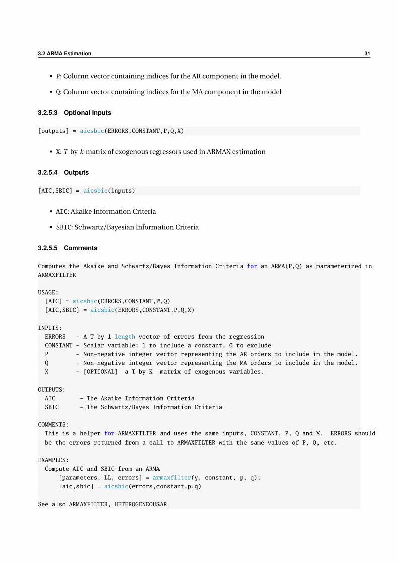
3.2.5.5 Comments
Computes the Akaike and Schwartz/Bayes Information Criteria for an ARMA(P,Q) as parameterized in
ARMAXFILTER
USAGE:
[AIC] = aicsbic(ERRORS,CONSTANT,P,Q)
[AIC,SBIC] = aicsbic(ERRORS,CONSTANT,P,Q,X)
INPUTS:
ERRORS - A T by 1 length vector of errors from the regression
CONSTANT - Scalar variable: 1 to include a constant, 0 to exclude
P - Non-negative integer vector representing the AR orders to include in the model.
Q - Non-negative integer vector representing the MA orders to include in the model.
X - [OPTIONAL] a T by K matrix of exogenous variables.
OUTPUTS:
AIC - The Akaike Information Criteria
SBIC - The Schwartz/Bayes Information Criteria
COMMENTS:
This is a helper for ARMAXFILTER and uses the same inputs, CONSTANT, P, Q and X. ERRORS should
be the errors returned from a call to ARMAXFILTER with the same values of P, Q, etc.
EXAMPLES:
Compute AIC and SBIC from an ARMA
[parameters, LL, errors] = armaxfilter(y, constant, p, q);
[aic,sbic] = aicsbic(errors,constant,p,q)
See also ARMAXFILTER, HETEROGENEOUSAR
32 Stationary Time Series
3.3 ARMA Forecasting
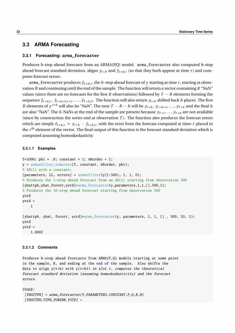
3.3.1 Forecasting: arma_forecaster
Produces h-step ahead forecasts from an ARMA(P,Q) model. arma_forecaster also computed h-step
ahead forecast standard deviation, aligns yt+h and yt+h |t (so that they both appear at time t ) and com-
putes forecast errors.
arma_forecaster produces yt+h |t , the h-step ahead forecast of y starting at time t , starting at obser-
vation R and continuing until the end of the sample. The function will return a vector containing R “NaN”
values (since there are no forecasts for the first R observations) followed by T − R elements forming the
sequence yr+h |r , yr+h+1|r+1, . . . , yT+h |T . The function will also return yt+h shifted back h places. The first
R elements of y t+h will also be “NaN”. The next T − R − h will be yr+h , yr+h+1, . . . , yT+h and the final h
are also “NaN”. The h-NaNs at the end of the sample are present because yT+1, . . . yT+h are not available
(since by construction the series end at observation T ). The function also produces the forecast errors
which are simply et+h |t = yt+h − yt+h |t , with the error from the forecast computed at time-t placed in
the t th element of the vector. The final output of this function is the forecast standard deviation which is
computed assuming homoskedasticity
3.3.1.1 Examples
T=1000; phi = .9; constant = 1; ARorder = 1;
y = armaxfilter_simulate(T, constant, ARorder, phi);
% AR(1) with a constant;
[parameters, LL, errors] = armaxfilter(y(1:500), 1, 1, 0);
% Produces the 1-step ahead forecast from an AR(1) starting from observation 500
[yhattph,yhat,forerr,ystd]=arma_forecaster(y,parameters,1,1,[],500,1);
% Produces the 10-step ahead forecast starting from observation 500
ystd
ystd =
1
[yhattph, yhat, forerr, ystd]=arma_forecaster(y, parameters, 1, 1, [] , 500, 10, 1);
ystd
ystd =
1.9002
3.3.1.2 Comments
Produces h-step ahead forecasts from ARMA(P,Q) models starting at some point
in the sample, R, and ending at the end of the sample. Also shifts the
data to align y(t+h) with y(t+ht) in slot t, computes the theoretical
forecast standard deviation (assuming homoskedasticity) and the forecast
errors.
USAGE:
[YHATTPH] = arma_forecaster(Y,PARAMETERS,CONSTANT,P,Q,R,H)
[YHATTPH,YTPH,FORERR,YSTD] =
3.3 ARMA Forecasting 33
arma_forecaster(Y,PARAMETERS,CONSTANT,P,Q,R,H,SEREGRESSION)
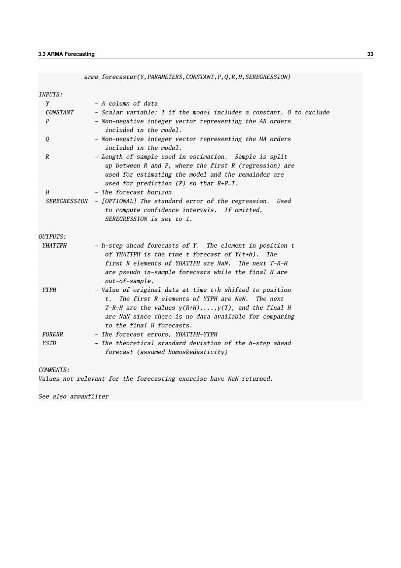
INPUTS:
Y - A column of data
CONSTANT - Scalar variable: 1 if the model includes a constant, 0 to exclude
P - Non-negative integer vector representing the AR orders
included in the model.
Q - Non-negative integer vector representing the MA orders
included in the model.
R - Length of sample used in estimation. Sample is split
up between R and P, where the first R (regression) are
used for estimating the model and the remainder are
used for prediction (P) so that R+P=T.
H - The forecast horizon
SEREGRESSION - [OPTIONAL] The standard error of the regression. Used
to compute confidence intervals. If omitted,
SEREGRESSION is set to 1.
OUTPUTS:
YHATTPH - h-step ahead forecasts of Y. The element in position t
of YHATTPH is the time t forecast of Y(t+h). The
first R elements of YHATTPH are NaN. The next T-R-H
are pseudo in-sample forecasts while the final H are
out-of-sample.
YTPH - Value of original data at time t+h shifted to position
t. The first R elements of YTPH are NaN. The next
T-R-H are the values y(R+H),...,y(T), and the final H
are NaN since there is no data available for comparing
to the final H forecasts.
FORERR - The forecast errors, YHATTPH-YTPH
YSTD - The theoretical standard deviation of the h-step ahead
forecast (assumed homoskedasticity)
COMMENTS:
Values not relevant for the forecasting exercise have NaN returned.
See also armaxfilter
34 Stationary Time Series
3.4 Sample autocorrelation and partial autocorrelation
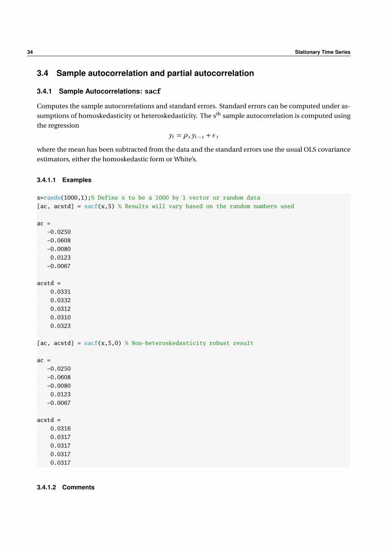
3.4.1 Sample Autocorrelations: sacf
Computes the sample autocorrelations and standard errors. Standard errors can be computed under as-
sumptions of homoskedasticity or heteroskedasticity. The sth sample autocorrelation is computed using
the regression
yt = ρs yt−s + εt
where the mean has been subtracted from the data and the standard errors use the usual OLS covariance
estimators, either the homoskedastic form or White’s.
3.4.1.1 Examples
x=randn(1000,1);% Define x to be a 1000 by 1 vector or random data
[ac, acstd] = sacf(x,5) % Results will vary based on the random numbers used
ac =
-0.0250
-0.0608
-0.0080
0.0123
-0.0067
acstd =
0.0331
0.0332
0.0312
0.0310
0.0323
[ac, acstd] = sacf(x,5,0) % Non-heteroskedasticity robust result
ac =
-0.0250
-0.0608
-0.0080
0.0123
-0.0067
acstd =
0.0316
0.0317
0.0317
0.0317
0.0317
3.4.1.2 Comments
3.4 Sample autocorrelation and partial autocorrelation 35
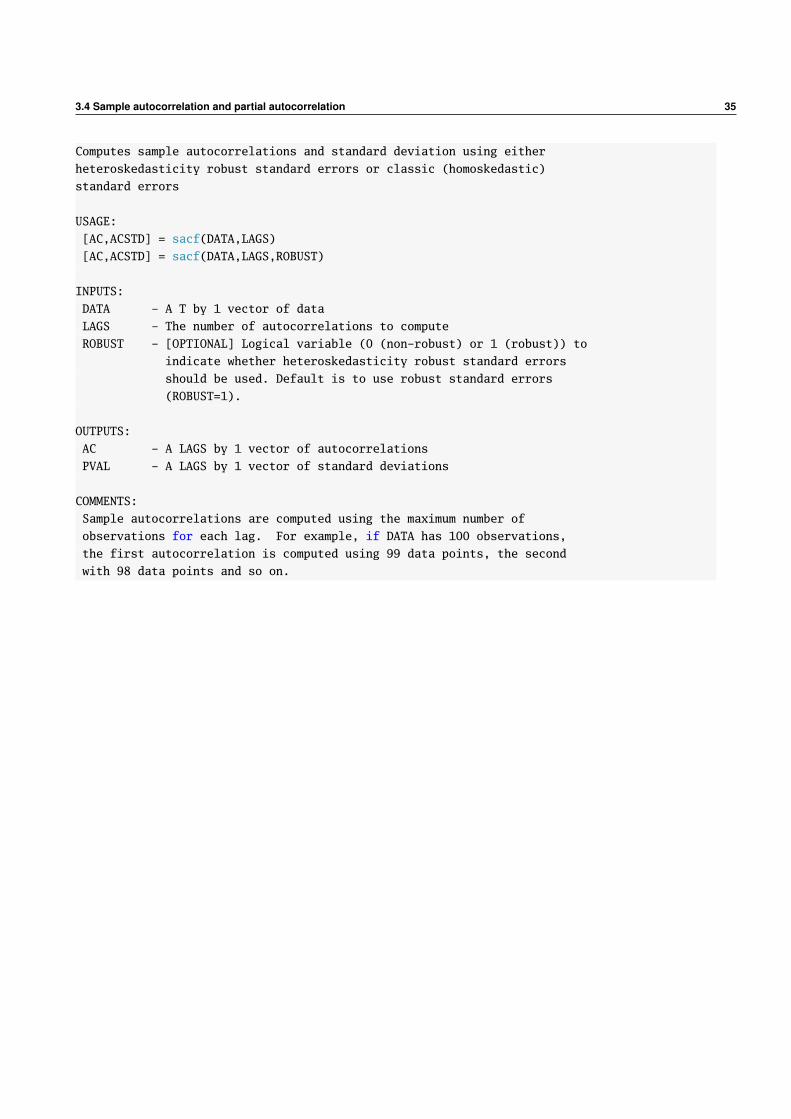
Computes sample autocorrelations and standard deviation using either
heteroskedasticity robust standard errors or classic (homoskedastic)
standard errors
USAGE:
[AC,ACSTD] = sacf(DATA,LAGS)
[AC,ACSTD] = sacf(DATA,LAGS,ROBUST)
INPUTS:
DATA - A T by 1 vector of data
LAGS - The number of autocorrelations to compute
ROBUST - [OPTIONAL] Logical variable (0 (non-robust) or 1 (robust)) to
indicate whether heteroskedasticity robust standard errors
should be used. Default is to use robust standard errors
(ROBUST=1).
OUTPUTS:
AC - A LAGS by 1 vector of autocorrelations
PVAL - A LAGS by 1 vector of standard deviations
COMMENTS:
Sample autocorrelations are computed using the maximum number of
observations for each lag. For example, if DATA has 100 observations,
the first autocorrelation is computed using 99 data points, the second
with 98 data points and so on.
36 Stationary Time Series
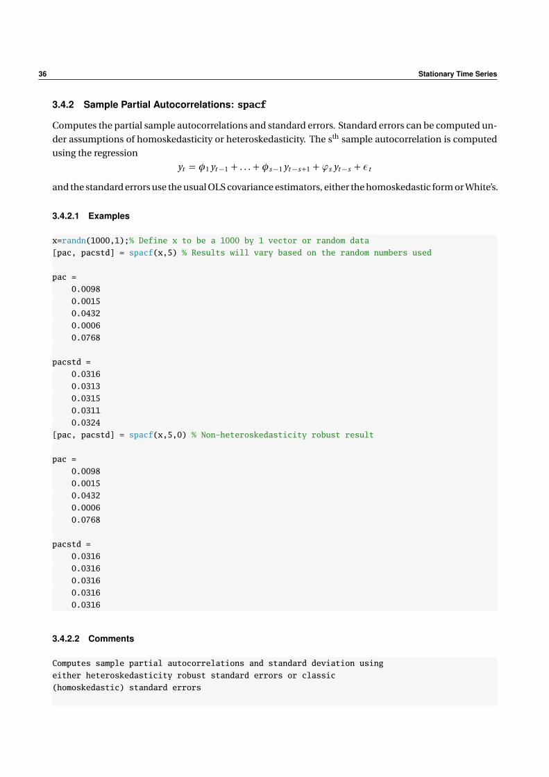
3.4.2 Sample Partial Autocorrelations: spacf
Computes the partial sample autocorrelations and standard errors. Standard errors can be computed un-
der assumptions of homoskedasticity or heteroskedasticity. The sth sample autocorrelation is computed
using the regression
yt = φ1 yt−1 + . . . + φs−1 yt−s+1 + ϕs yt−s + εt
and the standard errors use the usual OLS covariance estimators, either the homoskedastic form or White’s.
3.4.2.1 Examples
x=randn(1000,1);% Define x to be a 1000 by 1 vector or random data
[pac, pacstd] = spacf(x,5) % Results will vary based on the random numbers used
pac =
0.0098
0.0015
0.0432
0.0006
0.0768
pacstd =
0.0316
0.0313
0.0315
0.0311
0.0324
[pac, pacstd] = spacf(x,5,0) % Non-heteroskedasticity robust result
pac =
0.0098
0.0015
0.0432
0.0006
0.0768
pacstd =
0.0316
0.0316
0.0316
0.0316
0.0316
3.4.2.2 Comments
Computes sample partial autocorrelations and standard deviation using
either heteroskedasticity robust standard errors or classic
(homoskedastic) standard errors
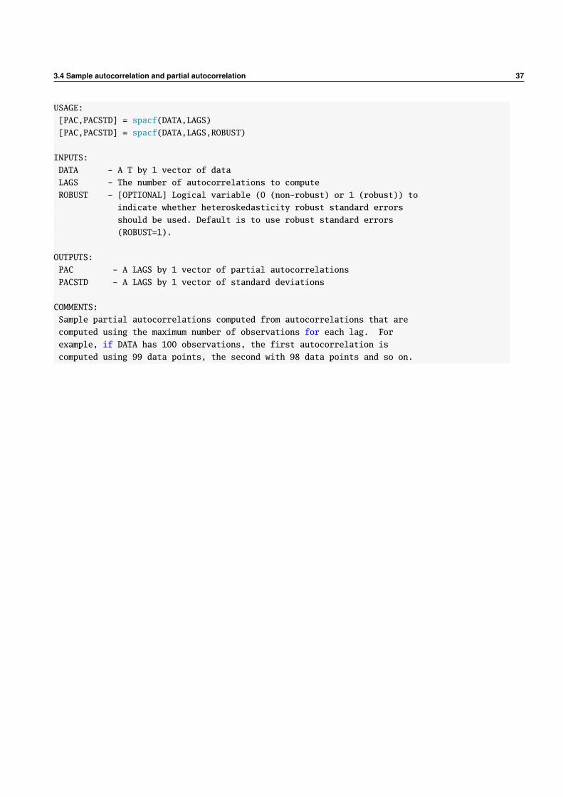
3.4 Sample autocorrelation and partial autocorrelation 37
USAGE:
[PAC,PACSTD] = spacf(DATA,LAGS)
[PAC,PACSTD] = spacf(DATA,LAGS,ROBUST)
INPUTS:
DATA - A T by 1 vector of data
LAGS - The number of autocorrelations to compute
ROBUST - [OPTIONAL] Logical variable (0 (non-robust) or 1 (robust)) to
indicate whether heteroskedasticity robust standard errors
should be used. Default is to use robust standard errors
(ROBUST=1).
OUTPUTS:
PAC - A LAGS by 1 vector of partial autocorrelations
PACSTD - A LAGS by 1 vector of standard deviations
COMMENTS:
Sample partial autocorrelations computed from autocorrelations that are
computed using the maximum number of observations for each lag. For
example, if DATA has 100 observations, the first autocorrelation is
computed using 99 data points, the second with 98 data points and so on.
38 Stationary Time Series
3.5 Theoretical autocorrelation and partial autocorrelation
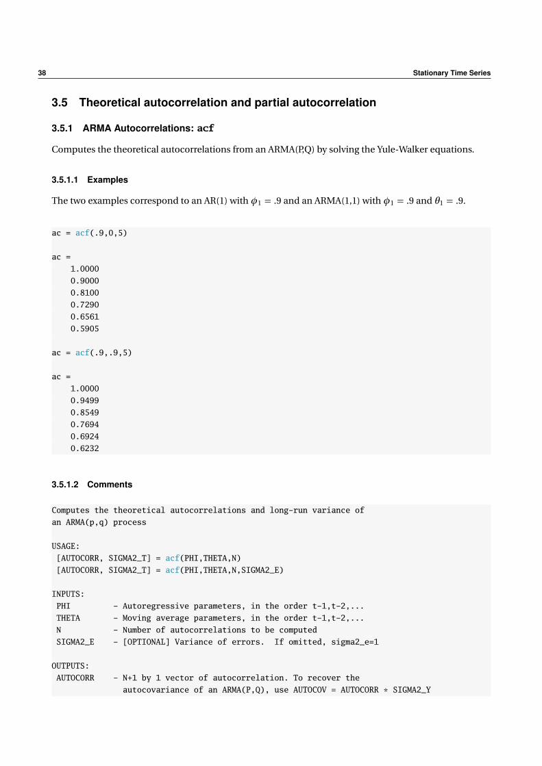
3.5.1 ARMA Autocorrelations: acf
Computes the theoretical autocorrelations from an ARMA(P,Q) by solving the Yule-Walker equations.
3.5.1.1 Examples
The two examples correspond to an AR(1) withφ1 = .9 and an ARMA(1,1) withφ1 = .9 and θ1 = .9.
ac = acf(.9,0,5)
ac =
1.0000
0.9000
0.8100
0.7290
0.6561
0.5905
ac = acf(.9,.9,5)
ac =
1.0000
0.9499
0.8549
0.7694
0.6924
0.6232
3.5.1.2 Comments
Computes the theoretical autocorrelations and long-run variance of
an ARMA(p,q) process
USAGE:
[AUTOCORR, SIGMA2_T] = acf(PHI,THETA,N)
[AUTOCORR, SIGMA2_T] = acf(PHI,THETA,N,SIGMA2_E)
INPUTS:
PHI - Autoregressive parameters, in the order t-1,t-2,...
THETA - Moving average parameters, in the order t-1,t-2,...
N - Number of autocorrelations to be computed
SIGMA2_E - [OPTIONAL] Variance of errors. If omitted, sigma2_e=1
OUTPUTS:
AUTOCORR - N+1 by 1 vector of autocorrelation. To recover the
autocovariance of an ARMA(P,Q), use AUTOCOV = AUTOCORR * SIGMA2_Y

3.5 Theoretical autocorrelation and partial autocorrelation 39
SIGMA2_Y - Long-run variance, denoted gamma0 of ARMA process with
innovation variance SIGMS2_E
COMMENTS:
Note: The ARMA model is parameterized as follows:
y(t)=phi(1)y(t-1)+phi(2)y(t-2)+...+phi(p)y(t-p)+e(t)+theta(1)e(t-1)
+theta(2)e(t-2)+...+theta(q)e(t-q)
To compute the autocorrelations for an ARMA that does not include all
lags 1 to P, insert 0 for any excluded lag. For example, if the model
was y(t) = phi(2)y(t-1), THETA = [0 phi(2)]
40 Stationary Time Series
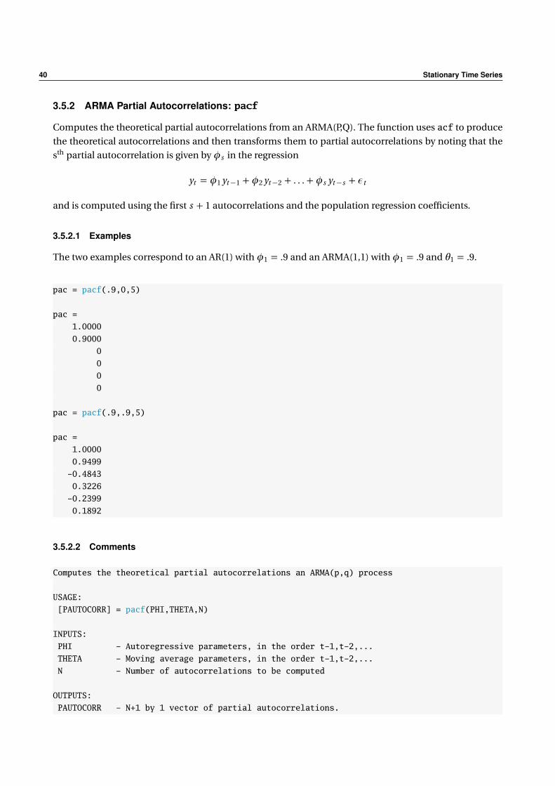
3.5.2 ARMA Partial Autocorrelations: pacf
Computes the theoretical partial autocorrelations from an ARMA(P,Q). The function uses acf to produce
the theoretical autocorrelations and then transforms them to partial autocorrelations by noting that the
sth partial autocorrelation is given byφs in the regression
yt = φ1 yt−1 + φ2 yt−2 + . . . + φs yt−s + εt
and is computed using the first s + 1 autocorrelations and the population regression coefficients.
3.5.2.1 Examples
The two examples correspond to an AR(1) withφ1 = .9 and an ARMA(1,1) withφ1 = .9 and θ1 = .9.
pac = pacf(.9,0,5)
pac =
1.0000
0.9000
0
0
0
0
pac = pacf(.9,.9,5)
pac =
1.0000
0.9499
-0.4843
0.3226
-0.2399
0.1892
3.5.2.2 Comments
Computes the theoretical partial autocorrelations an ARMA(p,q) process
USAGE:
[PAUTOCORR] = pacf(PHI,THETA,N)
INPUTS:
PHI - Autoregressive parameters, in the order t-1,t-2,...
THETA - Moving average parameters, in the order t-1,t-2,...
N - Number of autocorrelations to be computed
OUTPUTS:
PAUTOCORR - N+1 by 1 vector of partial autocorrelations.

3.5 Theoretical autocorrelation and partial autocorrelation 41
COMMENTS:
Note: The ARMA model is parameterized as follows:
y(t)=phi(1)y(t-1)+phi(2)y(t-2)+...+phi(p)y(t-p)+e(t)+theta(1)e(t-1)
+theta(2)e(t-2)+...+theta(q)e(t-q)
To compute the autocorrelations for an ARMA that does not include all
lags 1 to P, insert 0 for any excluded lag. For example, if the model
was y(t) = phi(2)y(t-1), THETA = [0 phi(2)]
42 Stationary Time Series
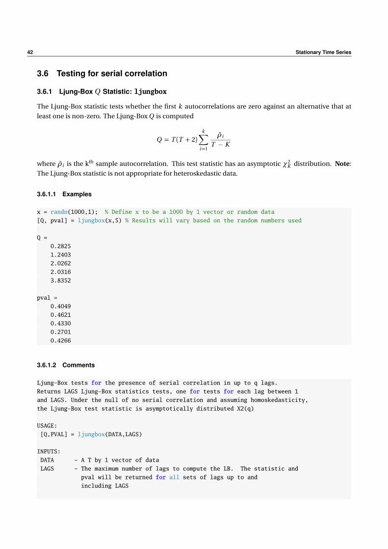
3.6 Testing for serial correlation
3.6.1 Ljung-Box Q Statistic: ljungbox
The Ljung-Box statistic tests whether the first k autocorrelations are zero against an alternative that at
least one is non-zero. The Ljung-Box Q is computed
Q = T (T + 2)k∑
i=1
ρi
T − K
where ρi is the kth sample autocorrelation. This test statistic has an asymptotic χ2K distribution. Note:
The Ljung-Box statistic is not appropriate for heteroskedastic data.
3.6.1.1 Examples
x = randn(1000,1); % Define x to be a 1000 by 1 vector or random data
[Q, pval] = ljungbox(x,5) % Results will vary based on the random numbers used
Q =
0.2825
1.2403
2.0262
2.0316
3.8352
pval =
0.4049
0.4621
0.4330
0.2701
0.4266
3.6.1.2 Comments
Ljung-Box tests for the presence of serial correlation in up to q lags.
Returns LAGS Ljung-Box statistics tests, one for tests for each lag between 1
and LAGS. Under the null of no serial correlation and assuming homoskedasticity,
the Ljung-Box test statistic is asymptotically distributed X2(q)
USAGE:
[Q,PVAL] = ljungbox(DATA,LAGS)
INPUTS:
DATA - A T by 1 vector of data
LAGS - The maximum number of lags to compute the LB. The statistic and
pval will be returned for all sets of lags up to and
including LAGS

3.6 Testing for serial correlation 43
OUTPUTS:
Q - A LAGS by 1 vector of Q statistics
PVAL - A LAGS by 1 set of appropriate pvals
COMMENTS:
This test statistic is common but often inappropriate since it assumes
homoskedasticity. For a heteroskedasticity consistent serial
correlation test, see lmtest1
SEE ALSO:
lmtest1, lmtest2
44 Stationary Time Series
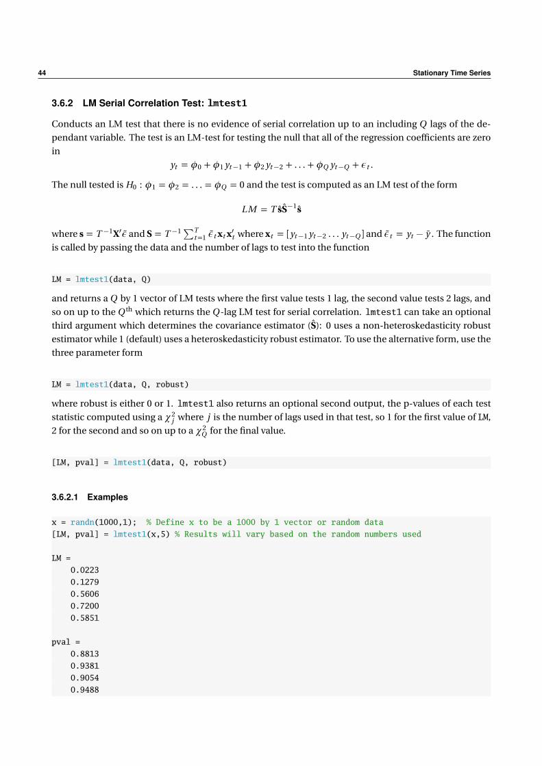
3.6.2 LM Serial Correlation Test: lmtest1
Conducts an LM test that there is no evidence of serial correlation up to an including Q lags of the de-
pendant variable. The test is an LM-test for testing the null that all of the regression coefficients are zero
in
yt = φ0 + φ1 yt−1 + φ2 yt−2 + . . . + φQ yt−Q + εt .
The null tested is H0 : φ1 = φ2 = . . . = φQ = 0 and the test is computed as an LM test of the form
LM = T sS−1s
where s = T −1X′ε and S = T −1∑Tt=1 εt xt x′t where xt = [yt−1 yt−2 . . . yt−Q ] and εt = yt − y . The function
is called by passing the data and the number of lags to test into the function
LM = lmtest1(data, Q)
and returns a Q by 1 vector of LM tests where the first value tests 1 lag, the second value tests 2 lags, and
so on up to the Q th which returns the Q -lag LM test for serial correlation. lmtest1 can take an optional
third argument which determines the covariance estimator (S): 0 uses a non-heteroskedasticity robust
estimator while 1 (default) uses a heteroskedasticity robust estimator. To use the alternative form, use the
three parameter form
LM = lmtest1(data, Q, robust)
where robust is either 0 or 1. lmtest1 also returns an optional second output, the p-values of each test
statistic computed using a χ2j where j is the number of lags used in that test, so 1 for the first value of LM,
2 for the second and so on up to a χ2Q for the final value.
[LM, pval] = lmtest1(data, Q, robust)
3.6.2.1 Examples
x = randn(1000,1); % Define x to be a 1000 by 1 vector or random data
[LM, pval] = lmtest1(x,5) % Results will vary based on the random numbers used
LM =
0.0223
0.1279
0.5606
0.7200
0.5851
pval =
0.8813
0.9381
0.9054
0.9488
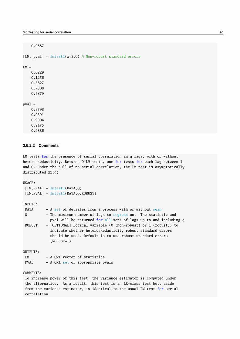
3.6 Testing for serial correlation 45
0.9887
[LM, pval] = lmtest1(x,5,0) % Non-robust standard errors
LM =
0.0229
0.1256
0.5827
0.7308
0.5879
pval =
0.8798
0.9391
0.9004
0.9475
0.9886
3.6.2.2 Comments
LM tests for the presence of serial correlation in q lags, with or without
heteroskedasticity. Returns Q LM tests, one for tests for each lag between 1
and Q. Under the null of no serial correlation, the LM-test is asymptotically
distributed X2(q)
USAGE:
[LM,PVAL] = lmtest1(DATA,Q)
[LM,PVAL] = lmtest1(DATA,Q,ROBUST)
INPUTS:
DATA - A set of deviates from a process with or without mean
Q - The maximum number of lags to regress on. The statistic and
pval will be returned for all sets of lags up to and including q
ROBUST - [OPTIONAL] Logical variable (0 (non-robust) or 1 (robust)) to
indicate whether heteroskedasticity robust standard errors
should be used. Default is to use robust standard errors
(ROBUST=1).
OUTPUTS:
LM - A Qx1 vector of statistics
PVAL - A Qx1 set of appropriate pvals
COMMENTS:
To increase power of this test, the variance estimator is computed under
the alternative. As a result, this test is an LR-class test but, aside
from the variance estimator, is identical to the usual LM test for serial
correlation
46 Stationary Time Series
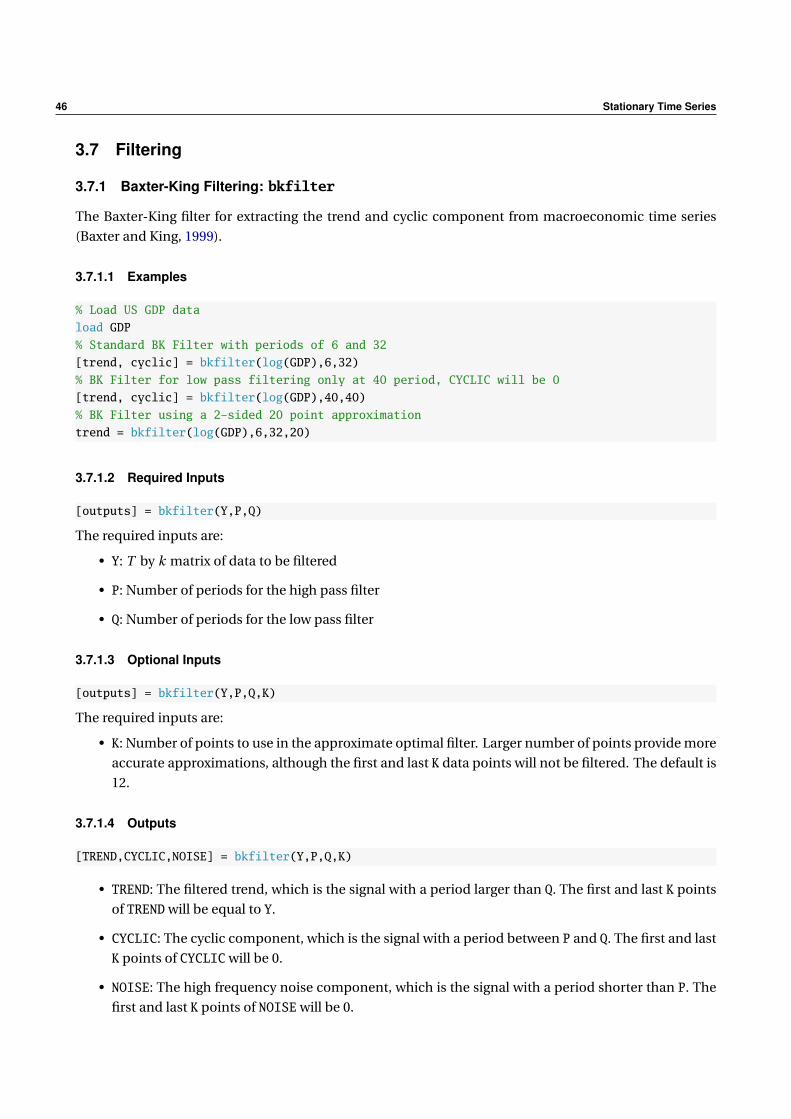
3.7 Filtering
3.7.1 Baxter-King Filtering: bkfilter
The Baxter-King filter for extracting the trend and cyclic component from macroeconomic time series
(Baxter and King, 1999).
3.7.1.1 Examples
% Load US GDP data
load GDP
% Standard BK Filter with periods of 6 and 32
[trend, cyclic] = bkfilter(log(GDP),6,32)
% BK Filter for low pass filtering only at 40 period, CYCLIC will be 0
[trend, cyclic] = bkfilter(log(GDP),40,40)
% BK Filter using a 2-sided 20 point approximation
trend = bkfilter(log(GDP),6,32,20)
3.7.1.2 Required Inputs
[outputs] = bkfilter(Y,P,Q)
The required inputs are:
• Y: T by k matrix of data to be filtered
• P: Number of periods for the high pass filter
• Q: Number of periods for the low pass filter
3.7.1.3 Optional Inputs
[outputs] = bkfilter(Y,P,Q,K)
The required inputs are:
• K: Number of points to use in the approximate optimal filter. Larger number of points provide more
accurate approximations, although the first and last K data points will not be filtered. The default is
12.
3.7.1.4 Outputs
[TREND,CYCLIC,NOISE] = bkfilter(Y,P,Q,K)
• TREND: The filtered trend, which is the signal with a period larger than Q. The first and last K points
of TREND will be equal to Y.
• CYCLIC: The cyclic component, which is the signal with a period between P and Q. The first and last
K points of CYCLIC will be 0.
• NOISE: The high frequency noise component, which is the signal with a period shorter than P. The
first and last K points of NOISE will be 0.
3.7 Filtering 47
3.7.1.5 Comments
Baxter-King filtering of multiple time series
USAGE:
[TREND,CYCLIC,NOISE] = bkfilter(Y,P,Q,K)
INPUTS:
Y - A T by K matrix of data to be filtered.
P - Number of periods to use in the higher frequency filter (e.g. 6 for quarterly data).
Must be at least 2.
Q - Number of periods to use in the lower frequency filter (e.g. 32 for quarterly data). Q
can be inf, in which case the low pass filter is a 2K+1 moving average.
K - [OPTIONAL] Number of points to use in the finite approximation bandpass filter. The
default value is 12. The filter throws away the first and last K points.
OUTPUTS:
TREND - A T by K matrix containing the filtered trend. The first and last K points equal Y.
CYCLIC - A T by K matrix containing the filtered cyclic component. The first and last K points are 0.
NOISE - A T by K matrix containing the filtered noise component. The first and last K points are 0.
COMMENTS:
The noise component is simply the original data minus the trend and cyclic component, NOISE = Y -
TREND - CYCLIC where the trend is produces by the low pass filter and the cyclic component is
produced by the difference of the high pass filter and the low pass filter. The recommended
values of P and Q are 6 and 32 or 40 for quarterly data, or 18 and 96 or 120 for monthly data.
Setting Q=P produces a single bandpass filer and the cyclic component will be 0.
EXAMPLES:
Load US GDP data
load GDP
Standard BK Filter with periods of 6 and 32
[trend, cyclic] = bkfilter(log(GDP),6,32)
BK Filter for low pass filtering only at 40 period, CYCLIC will be 0
[trend, cyclic] = bkfilter(log(GDP),40,40)
BK Filter using a 2-sided 20 point approximation
trend = bkfilter(log(GDP),6,32,20)
See also HP_FILTER, BEVERIDGENELSON
48 Stationary Time Series
3.7.2 Hodrick-Prescott Filtering: hp_filter
The Hodrick-Prescott filter for extracting the trend and cyclic component from macroeconomic time se-
ries (Hodrick and Prescott, 1997). The HP filter identifies the trend as the solution to
minµt
T∑t=1
(yt − µt )2 + λ (µt−1 − µt − µt + µt+1)
where λ is a parameter which determines the cutoff frequency of the filter and any trend points outside
of 1, . . . , T are dropped. If λ = 0 then µt = yt and as λ→∞ µt limits to a least squares linear trend fit.
3.7.2.1 Examples
% Load US GDP data
load GDP
% Standard HP Filter with lambda = 1600
[trend, cyclic] = hp_filter(log(GDP),1600)
3.7.2.2 Required Inputs
[outputs] = hp_filter(Y,LAMBDA)
The required inputs are:
• Y: T by k matrix of data to be filtered
• LAMBDA: Smoothing parameter for HP filter. Values above 1010 produce unstable matrix inverses
and so a linear trend is forced at this point.
3.7.2.3 Outputs
[TREND,CYCLIC] = hp_filter(inputs)
• TREND: The filtered trend.
• CYCLIC: The cyclic component.
3.7.2.4 Comments
Hodrick-Prescott filtering of multiple time series
USAGE:
[TREND,CYCLIC] = hp_filter(Y,LAMBDA)
INPUTS:
Y - A T by K matrix of data to be filtered.
LAMBDA - Positive, scalar integer containing the smoothing parameter of the HP filter.
3.7 Filtering 49
OUTPUTS:
TREND - A T by K matrix containing the filtered trend
CYCLIC - A T by K matrix containing the filtered cyclic component
COMMENTS:
The cyclic component is simply the original data minus the trend, CYCLIC = Y - TREND. 1600 is
the recommended value of LAMBDA for Quarterly Data while 14400 is the recommended value of LAMBDA
for monthly data.
EXAMPLES:
Load US GDP data
load GDP
Standard HP Filter with lambda = 1600
[trend, cyclic] = hp_filter(log(GDP),1600)
See also BKFILTER, BEVERIDGENELSON
50 Stationary Time Series
3.8 Regression with Time Series Data
3.8.1 Regression with time-series data: olsnw
Regression with Newey-West variance-covariance estimation. Aside from the difference variance-covariance
estimator, is virtually identical to ols.
3.8.1.1 Examples
% Set up some experimental data
T = 500;
e = armaxfilter_simulate(T,0,1,.8);
x = armaxfilter_simulate(T,0,1,.8);
y = x + e;
% Regression with a constant
b = olsnw(y,x)
% Regression through the origin (uncentered)
b = olsnw(y,x,0)
% Regression using 10 lags in the NW covariance estimator
b = olsnw(y,x,1,10)
3.8.1.2 Required Inputs
[outputs] = ols(Y,X)
The required inputs are:
• Y: A T by 1 vector containing the regressand.
• X: A T by k vector containing the regressors. X should be full rank and should not contain a constant
column.
3.8.1.3 Optional Inputs
[outputs] = olsnw(Y,X,C,NWLAGS)
The optional inputs are:
• C: A scalar (0 or 1) indicating whether the regression should include a constant. If 1 the X data are
augmented by a columns of 1s before the regression coefficients are estimated. If omitted or empty,
the default value is 1. C determines whether centered or uncentered estimators of R2and R2are com-
puted.
• NWLAGS: Number of lags to use when computing the variance-covariance matrix of the estimated
parameters. The default value is bT13 c.
3.8 Regression with Time Series Data 51
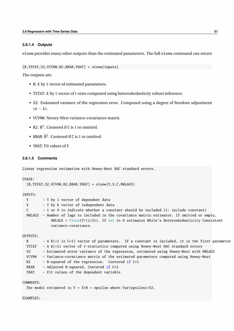
3.8.1.4 Outputs
olsnw provides many other outputs than the estimated parameters. The full olsnw command can return
[B,TSTAT,S2,VCVNW,R2,RBAR,YHAT] = olsnw(inputs)
The outputs are:
• B: k by 1 vector of estimated parameters.
• TSTAT: k by 1 vector of t-stats computed using heteroskedasticity robust inference.
• S2: Estimated variance of the regression error. Computed using a degree of freedom adjustment
(n − k ).
• VCVNW: Newey-West variance-covariance matrix
• R2: R2. Centered if C is 1 or omitted.
• RBAR: R2. Centered if C is 1 or omitted.
• YHAT: Fit values of Y
3.8.1.5 Comments
Linear regression estimation with Newey-West HAC standard errors.
USAGE:
[B,TSTAT,S2,VCVNW,R2,RBAR,YHAT] = olsnw(Y,X,C,NWLAGS)
INPUTS:
Y - T by 1 vector of dependent data
X - T by K vector of independent data
C - 1 or 0 to indicate whether a constant should be included (1: include constant)
NWLAGS - Number of lags to included in the covariance matrix estimator. If omitted or empty,
NWLAGS = floor(T^(1/3)). If set to 0 estimates White’s Heteroskedasticity Consistent
variance-covariance.
OUTPUTS:
B - A K(+1 is C=1) vector of parameters. If a constant is included, it is the first parameter
TSTAT - A K(+1) vector of t-statistics computed using Newey-West HAC standard errors
S2 - Estimated error variance of the regression, estimated using Newey-West with NWLAGS
VCVNW - Variance-covariance matrix of the estimated parameters computed using Newey-West
R2 - R-squared of the regression. Centered if C=1
RBAR - Adjusted R-squared. Centered if C=1
YHAT - Fit values of the dependent variable
COMMENTS:
The model estimated is Y = X*B + epsilon where Var(epsilon)=S2.
EXAMPLES:
52 Stationary Time Series
Regression with automatic BW selection
b = olsnw(y,x)
Regression without a constant
b = olsnw(y,x,0)
Regression with a pre-specified lag-length of 10
b = olsnw(y,x,1,10)
Regression with White standard errors
b = olsnw(y,x,1,0)
See also OLS
3.9 Long-run Covariance Estimation 53
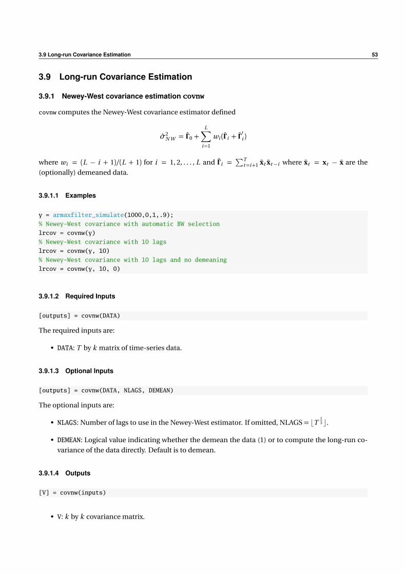
3.9 Long-run Covariance Estimation
3.9.1 Newey-West covariance estimation covnw
covnw computes the Newey-West covariance estimator defined
σ2N W = Γ 0 +
L∑i=1
wi (Γ i + Γ′i )
where wi = (L − i + 1)/(L + 1) for i = 1, 2, . . . , L and Γ i =∑T
t=i+1 xt xt−i where xt = xt − x are the
(optionally) demeaned data.
3.9.1.1 Examples
y = armaxfilter_simulate(1000,0,1,.9);
% Newey-West covariance with automatic BW selection
lrcov = covnw(y)
% Newey-West covariance with 10 lags
lrcov = covnw(y, 10)
% Newey-West covariance with 10 lags and no demeaning
lrcov = covnw(y, 10, 0)
3.9.1.2 Required Inputs
[outputs] = covnw(DATA)
The required inputs are:
• DATA: T by k matrix of time-series data.
3.9.1.3 Optional Inputs
[outputs] = covnw(DATA, NLAGS, DEMEAN)
The optional inputs are:
• NLAGS: Number of lags to use in the Newey-West estimator. If omitted, NLAGS = bT13 c.
• DEMEAN: Logical value indicating whether the demean the data (1) or to compute the long-run co-
variance of the data directly. Default is to demean.
3.9.1.4 Outputs
[V] = covnw(inputs)
• V: k by k covariance matrix.
54 Stationary Time Series
3.9.1.5 Comments
Long-run covariance estimation using Newey-West (Bartlett) weights
USAGE:
V = covnw(DATA)
V = covnw(DATA,NLAG,DEMEAN)
INPUTS:
DATA - T by K vector of dependent data
NLAG - Non-negative integer containing the lag length to use. If empty or not included,
NLAG=min(floor(1.2*T^(1/3)),T) is used
DEMEAN - Logical true or false (0 or 1) indicating whether the mean should be subtracted when
computing the covariance
OUTPUTS:
V - A K by K covariance matrix estimated using Newey-West (Bartlett) weights
COMMENTS:
EXAMPLES:
y = armaxfilter_simulate(1000,0,1,.9);
% Newey-West covariance with automatic BW selection
lrcov = covnw(y)
% Newey-West covariance with 10 lags
lrcov = covnw(y, 10)
% Newey-West covariance with 10 lags and no demeaning
lrcov = covnw(y, 10, 0)
See also COVVAR
3.9 Long-run Covariance Estimation 55
3.9.2 Den Hann-Levin covariance estimation covvar
Long-run covariance estimation using the VAR-based estimator of Haan and Levin 2000. The basic idea of
their estimator is the compute the long-run variance of a process from a Vector Autoregression. Suppose
a vector of data yt follows a stationary VAR,
(yt − µ) = Φ1 (yt−1 − µ) + . . . + Φk (yt−k − µ) + εt
where µ = E [yt ], then the variance of yt can be computed
(yt − µ)− Φ1 (yt−1 − µ)− . . .− Φk (yt−k − µ) = εt
from the VAR as
V [yt ] = [I− Φ1 − . . .− ΦK ]−1 Σ[
I− Φ′1 − . . .− Φ′K]−1
where Σ = E[εt ε′t
]is the unconditional covariance of the residuals (assumed to be a vector White Noise
process).
Note: This function differs slightly from the procedure of Den Haan and Levin in that it only conduct a
global lag length search, and so the resultant VAR will not have any zero elements. Den Haan and Levin
recommend using a series-by-series search with the possibility of having different lag lengths of own lags
and other lags. Changing to their procedure is something that may happen in future releases. Despite this
difference, the estimator in the code is still consistent as long as the maximum lag length
3.9.2.1 Examples
y = armaxfilter_simulate(1000,0,1,.9);
% VAR HAC covariance with automatic BW selection
lrcov = covvar(y)
% VAR HAC with at most 10 lags
lrcov = covvar(y, 10)
% VAR HAC with at most 10 lags selected using AIC
lrcov = covnw(y, 10, 3)
3.9.2.2 Required Inputs
[outputs] = covvar(DATA)
The required inputs are:
• DATA: T by k matrix of time-series data.
3.9.2.3 Optional Inputs
[outputs] = covnw(DATA, MAXLAGS, METHOD)
The optional inputs are:
• MAXLAGS: The maximum number of lags to consider when selecting the VAR lag length. If omitted is
set to b1.2T13 c or T /K , whichever is less.
56 Stationary Time Series
• METHOD: A scalar numeric value indicating the method to use when searching:
1. Use MAXLAGS in the VAR and do not search
2. Use up to MAXLAG and select the VAR order using SIC. This is the default.
3. Use up to MAXLAG and select the VAR order using AIC.
4. Use up to MAXLAG and select the VAR order using SIC using a global search. This option differs
from option 2 in that it can select an irregular VAR order (e.g. select lags 1 and 4 rather than 1,
2, 3 and 4.).
5. Use up to MAXLAG and select the VAR order using AIC using a global search.
3.9.2.4 Outputs
[V,LAGSUSED] = covvar(inputs)
• V: k by k covariance matrix.
• LAGSUSED: A vector indicating the lags used in estimating the covariance.
3.9.2.5 Comments
Long-run covariance estimation using Newey-West (Bartlett) weights
USAGE:
V = covnw(DATA)
V = covnw(DATA,NLAG,DEMEAN)
INPUTS:
DATA - T by K vector of dependent data
NLAG - Non-negative integer containing the lag length to use. If empty or not included,
NLAG=min(floor(1.2*T^(1/3)),T) is used
DEMEAN - Logical true or false (0 or 1) indicating whether the mean should be subtracted when
computing the covariance
OUTPUTS:
V - A K by K covariance matrix estimated using Newey-West (Bartlett) weights
COMMENTS:
EXAMPLES:
y = armaxfilter_simulate(1000,0,1,.9);
% Newey-West covariance with automatic BW selection
lrcov = covnw(y)
% Newey-West covariance with 10 lags
lrcov = covnw(y, 10)
% Newey-West covariance with 10 lags and no demeaning
lrcov = covnw(y, 10, 0)
See also COVVAR
Chapter 4
Nonstationary Time Series
4.1 Unit Root Testing
4.1.1 Augmented Dickey-Fuller testing: augdf
Estimates an Augmented Dickey-Fuller regression and returns the appropriate p-value for the assumption
made on the model and data generating process. The estimated model is
yt = α + ρyt−1 + γt + δ1∆yt−1 + ... + δP∆yt−p
The deterministic terms, α and γmay be included or excluded depending on which case it used and
the number of lags used in the estimation can be specified. augdf supports 4 cases:
• Case 0: DGP and estimated model contain no deterministic trends
• Case 1: DGP contains no deterministic time trend but estimated model includes a constant and a
time-trend
• Case 2: DGP contains a constant or a time trend. Estimated model includes both a constant and a
time trend.
• Case 3: DGP and estimated model contain a constant
A basic DF with no deterministic component can be estimated
[ADFstat, ADFpval] = augdf(y,0,0)
Other versions including lags in the ADF and deterministic trends can be estimated using
lags = 10; %set the number of ADF lags
p = 1;% Case 1
[ADFstat, ADFpval] = augdf(y,p,lags)
p = 2;
[ADFstat, ADFpval] = augdf(y,p,lags)
P-values were computed form 2 million simulations using gaussian errors. The function augdfcv returns
the appropriate critical values and p-values for the choice of case and size of the data sample (T ).
58 Nonstationary Time Series
4.1.1.1 Examples
x = cumsum(randn(1000,1)); % Define x to be a 1000 by 1 random walk
[ADFstat, ADFpval] = augdf(x,0,0) % Results will vary based rand. num. used
ADFstat =
-0.3941
ADFpval =
0.5472
[ADFstat, ADFpval] = augdf(x,1,0) % Assume a constant
ADFstat =
-2.3527
ADFpval =
0.1584
x = cumsum(1+randn(1000,1)); % Define x to be a 1000 by 1 random walk
% Case 3, Results will vary based on the random numbers used
[ADFstat, ADFpval] = augdf(x,3,0)
ADFstat =
0.6028
ADFpval =
0.7267
x = cumsum(randn(1000,1)); % Define x to be a 1000 by 1 random walk
[ADFstat, ADFpval, critval] = augdf(x,1,0) % Get the critical values
% for the 1%, 5%, 10%, 90%, 95% and 99% of the case-specific distribution
ADFstat =
-3.3738
ADFpval =
-0.0139
critval =
-3.4494
-2.8739
-2.5769
-0.4366
-0.0758
0.6123
4.1.1.2 Comments
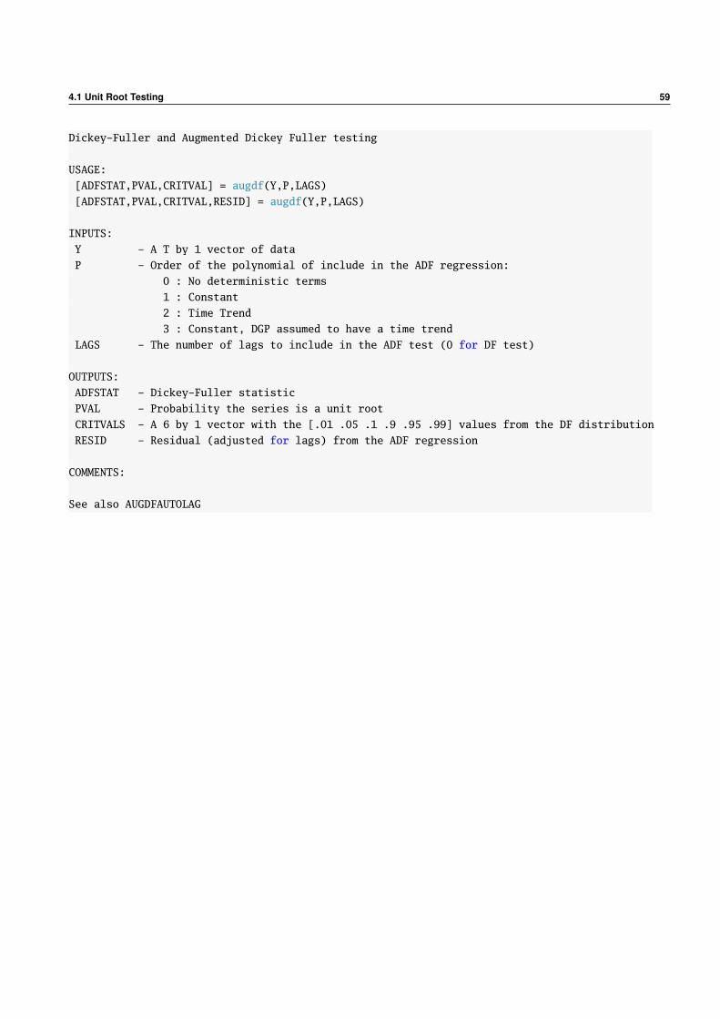
4.1 Unit Root Testing 59
Dickey-Fuller and Augmented Dickey Fuller testing
USAGE:
[ADFSTAT,PVAL,CRITVAL] = augdf(Y,P,LAGS)
[ADFSTAT,PVAL,CRITVAL,RESID] = augdf(Y,P,LAGS)
INPUTS:
Y - A T by 1 vector of data
P - Order of the polynomial of include in the ADF regression:
0 : No deterministic terms
1 : Constant
2 : Time Trend
3 : Constant, DGP assumed to have a time trend
LAGS - The number of lags to include in the ADF test (0 for DF test)
OUTPUTS:
ADFSTAT - Dickey-Fuller statistic
PVAL - Probability the series is a unit root
CRITVALS - A 6 by 1 vector with the [.01 .05 .1 .9 .95 .99] values from the DF distribution
RESID - Residual (adjusted for lags) from the ADF regression
COMMENTS:
See also AUGDFAUTOLAG
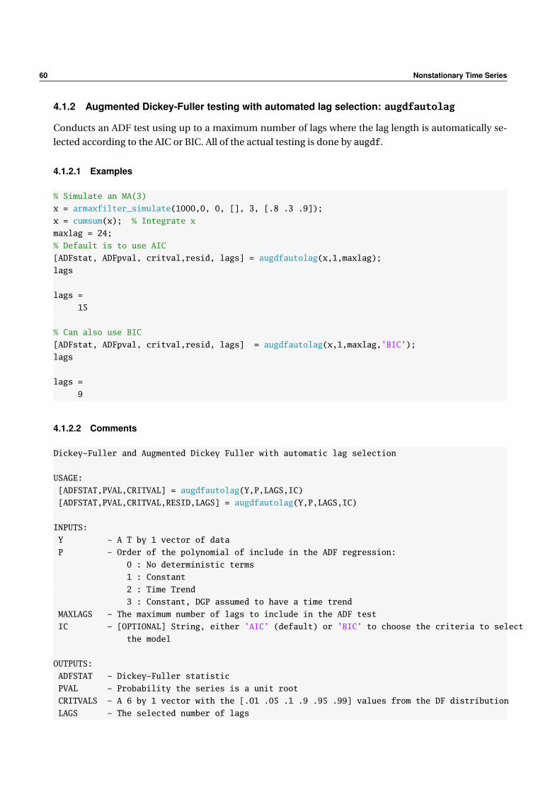
60 Nonstationary Time Series
4.1.2 Augmented Dickey-Fuller testing with automated lag selection: augdfautolag
Conducts an ADF test using up to a maximum number of lags where the lag length is automatically se-
lected according to the AIC or BIC. All of the actual testing is done by augdf.
4.1.2.1 Examples
% Simulate an MA(3)
x = armaxfilter_simulate(1000,0, 0, [], 3, [.8 .3 .9]);
x = cumsum(x); % Integrate x
maxlag = 24;
% Default is to use AIC
[ADFstat, ADFpval, critval,resid, lags] = augdfautolag(x,1,maxlag);
lags
lags =
15
% Can also use BIC
[ADFstat, ADFpval, critval,resid, lags] = augdfautolag(x,1,maxlag,’BIC’);
lags
lags =
9
4.1.2.2 Comments
Dickey-Fuller and Augmented Dickey Fuller with automatic lag selection
USAGE:
[ADFSTAT,PVAL,CRITVAL] = augdfautolag(Y,P,LAGS,IC)
[ADFSTAT,PVAL,CRITVAL,RESID,LAGS] = augdfautolag(Y,P,LAGS,IC)
INPUTS:
Y - A T by 1 vector of data
P - Order of the polynomial of include in the ADF regression:
0 : No deterministic terms
1 : Constant
2 : Time Trend
3 : Constant, DGP assumed to have a time trend
MAXLAGS - The maximum number of lags to include in the ADF test
IC - [OPTIONAL] String, either ’AIC’ (default) or ’BIC’ to choose the criteria to select
the model
OUTPUTS:
ADFSTAT - Dickey-Fuller statistic
PVAL - Probability the series is a unit root
CRITVALS - A 6 by 1 vector with the [.01 .05 .1 .9 .95 .99] values from the DF distribution
LAGS - The selected number of lags

4.1 Unit Root Testing 61
COMMENTS:
See also AUGDF

62 Nonstationary Time Series
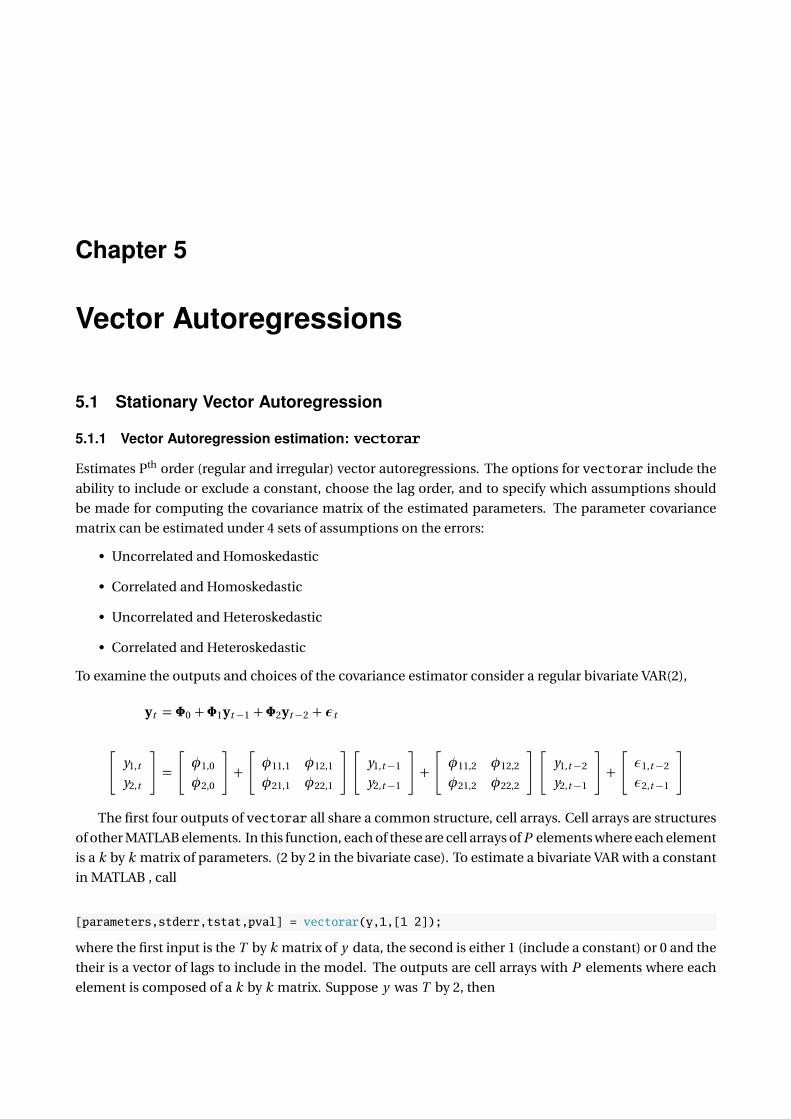
Chapter 5
Vector Autoregressions
5.1 Stationary Vector Autoregression
5.1.1 Vector Autoregression estimation: vectorar
Estimates Pth order (regular and irregular) vector autoregressions. The options for vectorar include the
ability to include or exclude a constant, choose the lag order, and to specify which assumptions should
be made for computing the covariance matrix of the estimated parameters. The parameter covariance
matrix can be estimated under 4 sets of assumptions on the errors:
• Uncorrelated and Homoskedastic
• Correlated and Homoskedastic
• Uncorrelated and Heteroskedastic
• Correlated and Heteroskedastic
To examine the outputs and choices of the covariance estimator consider a regular bivariate VAR(2),
yt = Φ0 + Φ1yt−1 + Φ2yt−2 + εt
[y1,t
y2,t
]=
[φ1,0
φ2,0
]+
[φ11,1 φ12,1
φ21,1 φ22,1
][y1,t−1
y2,t−1
]+
[φ11,2 φ12,2
φ21,2 φ22,2
][y1,t−2
y2,t−1
]+
[ε1,t−2
ε2,t−1
]
The first four outputs of vectorar all share a common structure, cell arrays. Cell arrays are structures
of other MATLAB elements. In this function, each of these are cell arrays of P elements where each element
is a k by k matrix of parameters. (2 by 2 in the bivariate case). To estimate a bivariate VAR with a constant
in MATLAB , call
[parameters,stderr,tstat,pval] = vectorar(y,1,[1 2]);
where the first input is the T by k matrix of y data, the second is either 1 (include a constant) or 0 and the
their is a vector of lags to include in the model. The outputs are cell arrays with P elements where each
element is composed of a k by k matrix. Suppose y was T by 2, then

64 Vector Autoregressions
[parameters,stderr,tstat,pval] = vectorar(y,1,[1 2]);
parameters % Tells you this is a cell structure of 2 by 2s
parameters =
[2x2 double] [2x2 double]
parameters1 % Access Phi(1)
ans =
0.6885 0.1621
0.1038 0.7500
parameters2 % Access Phi(2)
ans =
0.0267 0.0473
0.0503 -0.0031
The elements of parameters are identical to the elements of Φ j above. Thus, the (i,j) element of Φ1 will be
contained n the (i,j) element of parameters1 and the (i,j) element of Φ2 will be in the (i,j) element of
parameters2. The other four outputs in the function call above return similar cell structures of standard
errors, T-statistics and the corresponding p-values, all with the same ordering.
The full call to vectorar returns some additional information including the complete parameter co-
variance matrix.
[parameters,stderr,tstat,pval,const,conststd,r2,errors,s2,paramvec,vcv] ...
= vectorar(y,1,[1 2]);
The new outputs have the following structure:
• const: k by 1 vector containingΦ0. If no constant is included in the model, this value will be empty
([]).
• conststd: k by 1 vector containing the standard errors or the estimated intercept parameters. If no
constant is included in the model, this value will be empty ([]).
• r2: k by 1 vector of R 2 values for each data vector, y1,y2,. . .,yK .
• errors: T by k matrix of estimated errors.
• s2: k by k matrix containing the estimated covariance matrix of the residuals, Σ.
• paramvec: A K× number of lags by 1 (no constant) or K× number of lags +1 by 1 (constant) vector
of estimated parameters. paramvec reports the elements as if you were reading across a VAR. In the
bivariate VAR above, the 10 elements of paramvec are
[φ1,0 φ11,1 φ12,1 φ11,2 φ12,2 φ2,0 φ21,1 φ22,1 φ21,2 φ22,2]′
• vcv: A square matrix where each dimension is as large as the length of paramvec. The covariance
matrix has the same order as the elements of paramvec. In the bivariate VAR, the (1,1) element of
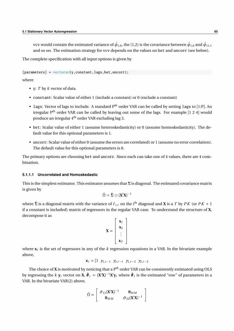
5.1 Stationary Vector Autoregression 65
vcv would contain the estimated variance of φ1,0, the (1,2) is the covariance between φ1,0 and φ11,1
and so on. The estimation strategy for vcv depends on the values on het and uncorr (see below).
The complete specification with all input options is given by
[parameters] = vectorar(y,constant,lags,het,uncorr);
where
• y: T by k vector of data.
• constant: Scalar value of either 1 (include a constant) or 0 (exclude a constant)
• lags: Vector of lags to include. A standard Pth order VAR can be called by setting lags to [1:P]. An
irregular Pth order VAR can be called by leaving out some of the lags. For example [1 2 4] would
produce an irregular 4th order VAR excluding lag 3.
• het: Scalar value of either 1 (assume heteroskedasticity) or 0 (assume homoskedasticity). The de-
fault value for this optional parameters is 1.
• uncorr: Scalar value of either 0 (assume the errors are correlated) or 1 (assume no error correlation).
The default value for this optional parameters is 0.
The primary options are choosing het and uncorr. Since each can take one of 4 values, there are 4 com-
bination.
5.1.1.1 Uncorrelated and Homoskedastic
This is the simplest estimator. This estimator assumes thatΣ is diagonal. The estimated covariance matrix
is given by
Ω = Σ⊗ (X′X)−1
where Σ is a diagonal matrix with the variance of εi ,t on the ith diagonal and X is a T by P K (or P K + 1
if a constant is included) matrix of regressors in the regular VAR case. To understand the structure of X,
decompose it as
X =
x1
x2...
xT
where x1 is the set of regressors in any of the k regression equations in a VAR. In the bivariate example
above,
xt = [1 y1,t−1 y2,t−1 y1,t−2 y2,t−2
The choice of X is motivated by noticing that a Pth order VAR can be consistently estimated using OLS
by regressing the k yi vector on X, θ i = (X′X)−1X′yi where θ i is the estimated “row” of parameters in a
VAR. In the bivariate VAR(2) above,
Ω =
[σ11(X′X)−1 0M M
0M M σ22(X′X)−1
]
66 Vector Autoregressions
where σi i is the estimated variance of εi ,t . and M is the length of xt .
5.1.1.2 Correlated and Homoskedastic
The correlated homoskedastic case is similar to the previous case with the change that Σ is no longer
assumed to be diagonal. Once this change has been made, the variance covariance estimator is identical
Ω = Σ⊗ (X′X)−1
In the bivariate VAR(2) above,
Ω =
[σ11(X′X)−1 σ12(X′X)−1
σ21(X′X)−1 σ22(X′X)−1
]where σi j is the estimated covariance between εi ,t and ε j ,t and σ12 = σ21.
5.1.1.3 Uncorrelated and Heteroskedastic
When residuals are heteroskedastic a White (or sandwich) -style covariance estimator is required. The two
parts of the sandwich are denoted A and B. A is given by
A = (X′XT)⊗ IK
and
B = T −1T∑
t=1
εt ε′t ⊗ xt x′t
Once these two components have been computed,
Ω = T −1A−1BA−1
The assumption that the errors are uncorrelated in this form imposes that T −1∑Tt=1 εi ,t ε j ,t xt x′t
p→0M M and so B is a “block diagonal” matrix where all of the elements in the off diagonal blocks are 0. In the
bivariate VAR(2) above,
A =
[X′XT 0M M
0M MX′XT
]and
B =
[T −1∑T
t=1 ε21,t ⊗ xt x′t 0M M
0M M T −1∑Tt=1 ε
22,t ⊗ xt x′t
].
Finally the T −1 is present int he formula for Ω since A and B both converge to constants although the
variance of the estimated coefficients should be decreasing with T .
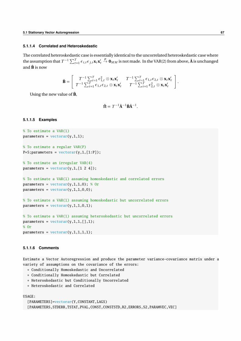
5.1 Stationary Vector Autoregression 67
5.1.1.4 Correlated and Heteroskedastic
The correlated heteroskedastic case is essentially identical to the uncorrelated heteroskedastic case where
the assumption that T −1∑Tt=1 εi ,t ε j ,t xt x′t
p→ 0M M is not made. In the VAR(2) from above, A is unchanged
and B is now
B =
[T −1∑T
t=1 ε21,t ⊗ xt x′t T −1∑T
t=1 ε1,t ε2,t ⊗ xt x′tT −1∑T
t=1 ε1,t ε2,t ⊗ xt x′t T −1∑Tt=1 ε
22,t ⊗ xt x′t
].
Using the new value of B,
Ω = T −1A−1BA−1.
5.1.1.5 Examples
% To estimate a VAR(1)
parameters = vectorar(y,1,1);
% To estimate a regular VAR(P)
P=5;parameters = vectorar(y,1,[1:P]);
% To estimate an irregular VAR(4)
parameters = vectorar(y,1,[1 2 4]);
% To estimate a VAR(1) assuming homoskedastic and correlated errors
parameters = vectorar(y,1,1,0); % Or
parameters = vectorar(y,1,1,0,0);
% To estimate a VAR(1) assuming homoskedastic but uncorrelated errors
parameters = vectorar(y,1,1,0,1);
% To estimate a VAR(1) assuming heteroskedastic but uncorrelated errors
parameters = vectorar(y,1,1,[],1);
% Or
parameters = vectorar(y,1,1,1,1);
5.1.1.6 Comments
Estimate a Vector Autoregression and produce the parameter variance-covariance matrix under a
variety of assumptions on the covariance of the errors:
* Conditionally Homoskedastic and Uncorrelated
* Conditionally Homoskedastic but Correlated
* Heteroskedastic but Conditionally Uncorrelated
* Heteroskedastic and Correlated
USAGE:
[PARAMETERS]=vectorar(Y,CONSTANT,LAGS)
[PARAMETERS,STDERR,TSTAT,PVAL,CONST,CONSTSTD,R2,ERRORS,S2,PARAMVEC,VEC]
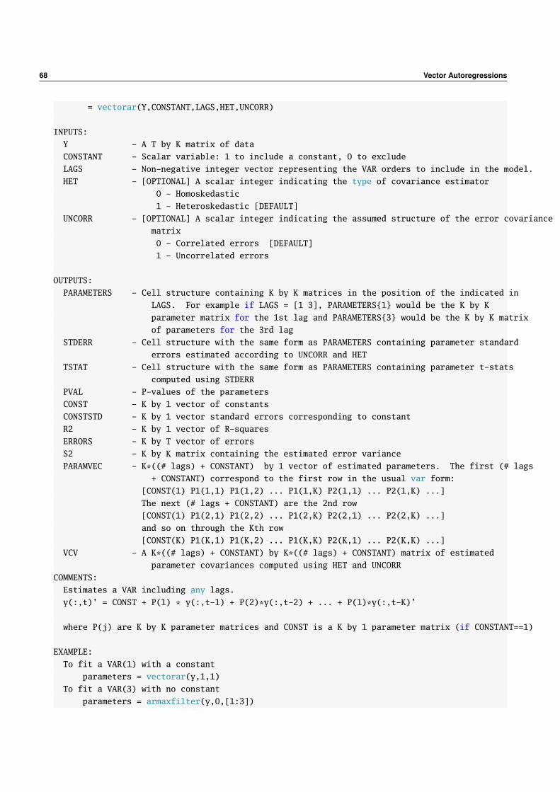
68 Vector Autoregressions
= vectorar(Y,CONSTANT,LAGS,HET,UNCORR)
INPUTS:
Y - A T by K matrix of data
CONSTANT - Scalar variable: 1 to include a constant, 0 to exclude
LAGS - Non-negative integer vector representing the VAR orders to include in the model.
HET - [OPTIONAL] A scalar integer indicating the type of covariance estimator
0 - Homoskedastic
1 - Heteroskedastic [DEFAULT]
UNCORR - [OPTIONAL] A scalar integer indicating the assumed structure of the error covariance
matrix
0 - Correlated errors [DEFAULT]
1 - Uncorrelated errors
OUTPUTS:
PARAMETERS - Cell structure containing K by K matrices in the position of the indicated in
LAGS. For example if LAGS = [1 3], PARAMETERS1 would be the K by K
parameter matrix for the 1st lag and PARAMETERS3 would be the K by K matrix
of parameters for the 3rd lag
STDERR - Cell structure with the same form as PARAMETERS containing parameter standard
errors estimated according to UNCORR and HET
TSTAT - Cell structure with the same form as PARAMETERS containing parameter t-stats
computed using STDERR
PVAL - P-values of the parameters
CONST - K by 1 vector of constants
CONSTSTD - K by 1 vector standard errors corresponding to constant
R2 - K by 1 vector of R-squares
ERRORS - K by T vector of errors
S2 - K by K matrix containing the estimated error variance
PARAMVEC - K*((# lags) + CONSTANT) by 1 vector of estimated parameters. The first (# lags
+ CONSTANT) correspond to the first row in the usual var form:
[CONST(1) P1(1,1) P1(1,2) ... P1(1,K) P2(1,1) ... P2(1,K) ...]
The next (# lags + CONSTANT) are the 2nd row
[CONST(1) P1(2,1) P1(2,2) ... P1(2,K) P2(2,1) ... P2(2,K) ...]
and so on through the Kth row
[CONST(K) P1(K,1) P1(K,2) ... P1(K,K) P2(K,1) ... P2(K,K) ...]
VCV - A K*((# lags) + CONSTANT) by K*((# lags) + CONSTANT) matrix of estimated
parameter covariances computed using HET and UNCORR
COMMENTS:
Estimates a VAR including any lags.
y(:,t)’ = CONST + P(1) * y(:,t-1) + P(2)*y(:,t-2) + ... + P(1)*y(:,t-K)’
where P(j) are K by K parameter matrices and CONST is a K by 1 parameter matrix (if CONSTANT==1)
EXAMPLE:
To fit a VAR(1) with a constant
parameters = vectorar(y,1,1)
To fit a VAR(3) with no constant
parameters = armaxfilter(y,0,[1:3])

5.1 Stationary Vector Autoregression 69
To fit a VAR that includes lags 1 and 3 with a constant
parameters = armaxfilter(y,1,[1 3])
See also IMPULSERESPONSE, GRANGERCAUSE, VECTORARVCV
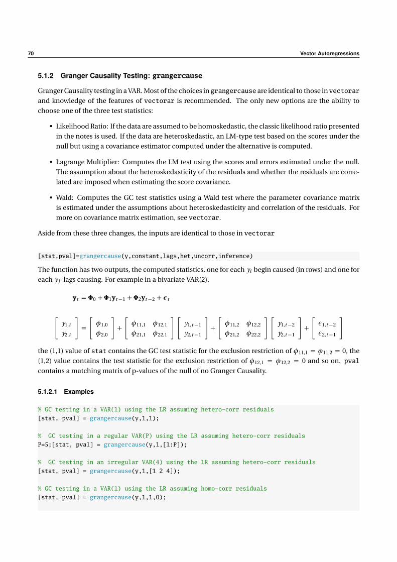
70 Vector Autoregressions
5.1.2 Granger Causality Testing: grangercause
Granger Causality testing in a VAR. Most of the choices ingrangercause are identical to those invectorar
and knowledge of the features of vectorar is recommended. The only new options are the ability to
choose one of the three test statistics:
• Likelihood Ratio: If the data are assumed to be homoskedastic, the classic likelihood ratio presented
in the notes is used. If the data are heteroskedastic, an LM-type test based on the scores under the
null but using a covariance estimator computed under the alternative is computed.
• Lagrange Multiplier: Computes the LM test using the scores and errors estimated under the null.
The assumption about the heteroskedasticity of the residuals and whether the residuals are corre-
lated are imposed when estimating the score covariance.
• Wald: Computes the GC test statistics using a Wald test where the parameter covariance matrix
is estimated under the assumptions about heteroskedasticity and correlation of the residuals. For
more on covariance matrix estimation, see vectorar.
Aside from these three changes, the inputs are identical to those in vectorar
[stat,pval]=grangercause(y,constant,lags,het,uncorr,inference)
The function has two outputs, the computed statistics, one for each yi begin caused (in rows) and one for
each yj -lags causing. For example in a bivariate VAR(2),
yt = Φ0 + Φ1yt−1 + Φ2yt−2 + εt
[y1,t
y2,t
]=
[φ1,0
φ2,0
]+
[φ11,1 φ12,1
φ21,1 φ22,1
][y1,t−1
y2,t−1
]+
[φ11,2 φ12,2
φ21,2 φ22,2
][y1,t−2
y2,t−1
]+
[ε1,t−2
ε2,t−1
]
the (1,1) value of stat contains the GC test statistic for the exclusion restriction of φ11,1 = φ11,2 = 0, the
(1,2) value contains the test statistic for the exclusion restriction of φ12,1 = φ12,2 = 0 and so on. pval
contains a matching matrix of p-values of the null of no Granger Causality.
5.1.2.1 Examples
% GC testing in a VAR(1) using the LR assuming hetero-corr residuals
[stat, pval] = grangercause(y,1,1);
% GC testing in a regular VAR(P) using the LR assuming hetero-corr residuals
P=5;[stat, pval] = grangercause(y,1,[1:P]);
% GC testing in an irregular VAR(4) using the LR assuming hetero-corr residuals
[stat, pval] = grangercause(y,1,[1 2 4]);
% GC testing in a VAR(1) using the LR assuming homo-corr residuals
[stat, pval] = grangercause(y,1,1,0);
5.1 Stationary Vector Autoregression 71
% GC testing in a VAR(1) using the LR assuming homo-uncorr residuals
[stat, pval] = grangercause(y,1,1,0,1);
% GC testing in a VAR(1) using the LR assuming hetero-uncorr residuals
[stat, pval] = grangercause(y,1,1,1,1);
% or
[stat, pval] = grangercause(y,1,1,[],1);
% GC testing in a VAR(1) using the LM assuming hetero-corr residuals
[stat, pval] = grangercause(y,1,1,1,0,2);
% or
[stat, pval] = grangercause(y,1,1,[],[],2);
% GC testing in a VAR(1) using the Wald assuming hetero-corr residuals
[stat, pval] = grangercause(y,1,1,1,0,3);
% or
[stat, pval] = grangercause(y,1,1,[],[],3);
5.1.2.2 Comments
Granger causality testing with a variance-covariance matrix estimated under a variety of
assumptions on the covariance of the errors:
* Conditionally Homoskedastic and Uncorrelated
* Conditionally Homoskedastic but Correlated
* Heteroskedastic but Conditionally Uncorrelated
* Heteroskedastic and Correlated
USAGE:
[STAT] = grangercause(Y,CONSTANT,LAGS)
[STAT,PVAL] = grangercause(Y,CONSTANT,LAGS,HET,UNCORR,INFERENCE)
INPUTS:
Y - A T by K matrix of data
CONSTANT - Scalar variable: 1 to include a constant, 0 to exclude
LAGS - Non-negative integer vector representing the VAR orders to include in the model.
HET - [OPTIONAL] A scalar integer indicating the type of covariance estimator
0 - Homoskedastic
1 - Heteroskedastic [DEFAULT]
UNCORR - [OPTIONAL] A scalar integer indicating the assumed structure of the error
covariance matrix
0 - Correlated errors [DEFAULT]
1 - Uncorrelated errors
INFERENCE - [OPTIONAL] Inference method
1 - Likelihood ratio
2 - LM test
3 - Wald test
72 Vector Autoregressions
OUTPUTS:
STAT - K by K matrix of Granger causality statistics computed using the specified
covariance estimator and inference method STAT(i,j) corresponds to a test that
y(i) is caused by y(j)
PVAL - K by K matrix of p-values corresponding to STAT
COMMENTS:
Granger causality tests based on a VAR including any lags.
y(:,t)’ = CONST + P(1) * y(:,y-1) + P(2)*y(:,y-2) + ... + P(1)*y(:,t-K)’
where P(j) are K by K parameter matrices and CONST is a K by 1 parameter matrix (if CONSTANT==1)
EXAMPLE:
Conduct GC testing in a VAR(1) with a constant
parameters = grangercause(y,1,1)
Conduct GC testing in a VAR(3) with no constant
parameters = grangercause(y,0,[1:3])
Conduct GC testing in a VAR that includes lags 1 and 3 with a constant
parameters = grangercause(y,1,[1 3])
See also VECTORAR, VECTORARVCV
5.1 Stationary Vector Autoregression 73
5.1.3 Impulse Response function calculation: impulseresponse
Impulse response function, standard errors and plotting. impulseresponsederives heavily fromvectorar
and uses much of the same syntax. The important new options to impulseresponse are the number if
impulses to compute, leads, and the assumption used for decomposing the error covariance, sqrttype.
impulseresponse always returns leads+1 impulses and standard errors since the 0th is included. leads
is a positive integer. sqrttype can be any one of:
• 0: Use non-scaled (unit) shocks
• 1: Use scaled but assume the correlation is zero. The scaling is the estimated standard deviation
from the VAR specification used. This is the default.
• 2: Use a Choleski decomposition.
• 3: Use a Spectral decomposition.
• k by k positive definite user provided square root matrix. This option was provided to allow the user
to impose a block spectral structure on the square root should they choose.
The general form of impulseresponse is
[impulses,impulsesstd,hfig] = impulseresponse(y,constant,lags,leads,...
sqrttype,graph,het,uncorr)
where y, constant, lags, het and uncorr are the same as in vectorar. leads and sqrttype are as de-
scribed above and graph is a 1 (produce plot) or 0 variable indicating whether a plot with 95% confidence
bands should be produced. The outputs are:
• impulses: A k by k by leads 3-D matrix of impulse responses. The element in position (i,j,l) is the
impulse response of yi to a shock to ε j , l -periods in the future.
• impulsesstd: A k by k by leads 3-D matrix of impulse response standard errors. These correspond
directly to the impulse response in the same position.
• hfig: A handle to the plot produced. Empty if graph is 0.
5.1.3.1 Examples
% 12 Impulse responses for a VAR(1) assuming hetero-corr residuals
[impulses,impulsesstd] = impulseresponse(y,1,1,12);
% 12 Impulse responses for a VAR(P) assuming hetero-corr residuals
P=5;[impulses,impulsesstd] = impulseresponse(y,1,1:P,12);
% 12 Impulse responses for am irregular VAR(P) assuming hetero-corr residuals
P=5;[impulses,impulsesstd] = impulseresponse(y,1,[1 2 4],12);
% 12 Impulse responses for a VAR(1), no graphs
[impulses,impulsesstd] = impulseresponse(y,1,1,12,[],0);
74 Vector Autoregressions
% 12 Impulse responses for a VAR(1), Choleski
[impulses,impulsesstd] = impulseresponse(y,1,1,12,2);
% 12 Impulse responses for a VAR(1), Spectral
[impulses,impulsesstd] = impulseresponse(y,1,1,12,3);
% 12 Impulse responses for a VAR(1), Unit shocks
[impulses,impulsesstd] = impulseresponse(y,1,1,12,0);
% 12 Impulse responses for a VAR(1), assuming homoskedastic, uncorrelated residuals
[impulses,impulsesstd] = impulseresponse(y,1,1,12,[],[],0,1);
5.1.3.2 Comments
Computes impulse responses for a VAR(P) or irregular VAR(P) and standard
errors under a variety of assumptions on the covariance of the errors:
* Conditionally Homoskedastic and Uncorrelated
* Conditionally Homoskedastic but Correlated
* Heteroskedastic but Conditionally Uncorrelated
* Heteroskedastic and Correlated
USAGE:
[IMPULSES]=impulseresponse(Y,CONSTANT,LAGS,LEADS)
[IMPULSES,IMPULSESTD,HFIG]=impulseresponse(Y,CONSTANT,LAGS,LEADS,SQRTTYPE,GRAPH,HET,UNCORR)
INPUTS:
Y - A T by K matrix of data
CONSTANT - Scalar variable: 1 to include a constant, 0 to exclude
LAGS - Non-negative integer vector representing the VAR orders to include in the model.
LEADS - Number of leads to compute the impulse response function
SQRTTYPE - [OPTIONAL] Either a scalar or a K by K positive definite matrix. This input
determines the type of covariance decomposition used. If it is a scalar if must
be one of:
0 - Unit (unscaled) shocks, covariance assumed to be an identity matrix
1 - [DEFAULT] Scaled but uncorrelated shocks. Scale is based on estimated
error standard deviations.
2 - Scaled and correlated shocks, Choleski decomposition. Scale is based on
estimated error standard deviations.
3 - Scaled and correlated shocks, spectral decomposition. Scale is based on
estimated error standard deviations.
If the input is a K by K positive definite matrix, it is used as the
covariance square root for computing the impulse response function.
GRAPH - [OPTIONAL] Logical variable (0 (no graph) or 1 (graph)) indicating whether the
function should produce a bar plot of the sample autocorrelations and confidence
intervals. Default is to produce a graphic (GRAPH=1).
HET - [OPTIONAL] A scalar integer indicating the type of
covariance estimator
0 - Homoskedastic
5.1 Stationary Vector Autoregression 75
1 - Heteroskedastic [DEFAULT]
UNCORR - [OPTIONAL] A scalar integer indicating the assumed structure of the error
covariance matrix
0 - Correlated errors [DEFAULT]
1 - Uncorrelated errors
OUTPUTS:
IMPULSES - Cell structure containing K by K matrices in the position of the indicated in
LAGS. For example if LAGS = [1 3], PARAMETERS1 would be the K by K parameter
matrix for the 1st lag and PARAMETERS3 would be the K by K matrix of
parameters for the 3rd lag
IMPULSESSTD - Cell structure containing K by K matrices in the containing parameter standard
errors estimated according to UNCORR and HET
HFIG - Figure handle to the bar plot of the autocorrelations
COMMENTS:
Estimates a VAR including any lags.
y(:,t)’ = CONST + P(1) * y(:,y-1) + P(2)*y(:,y-2) + ... + P(1)*y(:,t-K)’
where P(j) are K by K parameter matrices and CONST is a K by 1 parameter matrix (if CONSTANT==1)
EXAMPLE:
To produce the IR for 12 leads form a VAR(1) with a constant
impulses = impulserepsonse(y,1,1,12)
To produce the IR for 12 leads form a VAR(3) without a constant
impulses = impulserepsonse(y,0,[1:3],12)
To produce the IR for 12 leads form an irregular VAR(3) with only lags 1 and 3 with a constant
impulses = impulserepsonse(y,1,[1:3],12)
See also VECTORAR VECTORARVCV GRANGERCAUSE

76 Vector Autoregressions
Chapter 6
Volatility Modeling
6.1 GARCH Model Simulation
6.1.1 ARCH/GARCH/AVARCH/TARCH/ZARCH Simulation: tarch_simulate
ARCH/GARCH/AVARCH/TARCH/ZARCH model simulation with normal, Student’s t , Generalized Error
Distribution, Skew t or user supplied innovations.
6.1.1.1 Examples
% GARCH(1,1) simulation
simulatedData = tarch_simulate(1000, [1 .1 .8], 1, 0, 1)
% GJR-GARCH(1,1,1) simulation
simulatedData = tarch_simulate(1000, [1 .1 .1 .8], 1, 1, 1)
% GJR-GARCH(1,1,1) simulation with standardized Student’s T innovations
simulatedData = tarch_simulate(1000, [1 .1 .1 .8 6], 1, 1, 1, ’STUDENTST’)
% TARCH(1,1,1) simulation
simulatedData = tarch_simulate(1000, [1 .1 .1 .8], 1, 1, 1, [], 1)
6.1.1.2 Required Inputs
[outputs] = tarch_simulate(T, PARAMETERS, P, O, Q)
• T: Either a scalar integer or a vector of random numbers. If scalar, T represents the length of the
time series to simulate. If a T by 1 vector of random numbers, these will be used to construct the
simulated time series.
• PARAMETERS: 1 + P+O+Q by 1 vector of parameters in the order
[ωα1 . . . αP γ1 . . . γO β1 . . . βQ ]′
• P: Order of symmetric innovations in model
• O: Order of asymmetric innovations in model
• Q: Order of lagged variances in model
78 Volatility Modeling
6.1.1.3 Optional Inputs
[outputs] = tarch_simulate(T, PARAMETERS, P, O, Q, ERROR_TYPE, TARCH_TYPE)
• ERRORTYPE: Sting value indicating distribution of standardized shock.
– ’NORMAL’: Normal
– ’STUDENTST’: Standardized Student’s t . Parameters should contain 1 additional parameter
containing the shape of the distribution.
– ’GED’: Generalized Error Distribution. Parameters should contain 1 additional parameter con-
taining the shape of the distribution.
– ’SKEWT’: Skewed t . Parameters should contain 2 additional parameters containing the skew-
ness and tail parameters, with skewness first.
• TARCHTYPE: 1 for AVGARCH/TARCH/ZARCH, 2 for GARCH/GJR-GARCH. 2 is the default.
6.1.1.4 Outputs
[SIMULATEDATA, HT] = tarch_simulate(inputs)
• SIMULATEDATA: T by 1 vector of simulated data
• HT: T by 1 vector containing the conditional variance of the simulated data.
6.1.1.5 Comments
TARCH(P,O,Q) time series simulation with multiple error distributions
USAGE:
[SIMULATEDATA, HT] = tarch_simulate(T, PARAMETERS, P, O, Q, ERROR_TYPE, TARCH_TYPE)
INPUTS:
T - Length of the time series to be simulated OR
T by 1 vector of user supplied random numbers (i.e. randn(1000,1))
PARAMETERS - a 1+P+O+Q (+1 or 2, depending on error distribution) x 1 parameter vector
[omega alpha(1) ... alpha(p) gamma(1) ... gamma(o) beta(1) ... beta(q) [nu lambda]]’.
P - Positive, scalar integer representing the number of symmetric innovations
O - Non-negative scalar integer representing the number of asymmetric innovations (0
for symmetric processes)
Q - Non-negative, scalar integer representing the number of lags of conditional
variance (0 for ARCH)
ERROR_TYPE - [OPTIONAL] The error distribution used, valid types are:
’NORMAL’ - Gaussian Innovations [DEFAULT]
’STUDENTST’ - T distributed errors
’GED’ - Generalized Error Distribution
’SKEWT’ - Skewed T distribution
TARCH_TYPE - [OPTIONAL] The type of variance process, either
6.1 GARCH Model Simulation 79
1 - Model evolves in absolute values
2 - Model evolves in squares [DEFAULT]
OUTPUTS:
SIMULATEDATA - A time series with ARCH/GARCH/GJR/TARCH variances
HT - A vector of conditional variances used in making the time series
COMMENTS:
The conditional variance, h(t), of a TARCH(P,O,Q) process is modeled as follows:
g(h(t)) = omega
+ alpha(1)*f(r_t-1) + ... + alpha(p)*f(r_t-p)
+ gamma(1)*I(t-1)*f(r_t-1) +...+ gamma(o)*I(t-o)*f(r_t-o)
+ beta(1)*g(h(t-1)) +...+ beta(q)*g(h(t-q))
where f(x) = abs(x) if tarch_type=1
g(x) = sqrt(x) if tarch_type=1
f(x) = x^2 if tarch_type=2
g(x) = x if tarch_type=2
NOTE: This program generates 2000 more than required to minimize any starting bias
See also TARCH
80 Volatility Modeling
6.1.2 EGARCH Simulation: egarch_simulate
EGARCH simulation with normal, Student’s t , Generalized Error Distribution, Skew t or user supplied
innovations.
6.1.2.1 Examples
% Simulate a symmetric EGARCH(1,0,1) process
simulatedData = egarch_simulate(1000,[0 .1 .95],1,0,1);
% Simulate a standard EGARCH(1,1,1) process
simulatedData = egarch_simulate(1000,[0 .1 -.1 .95],1,1,1);
% Simulate a standard EGARCH(1,1,1) process with Student’s T innovations
simulatedData = egarch_simulate(1000,[0 .1 -.1 .95 6],1,1,1,’STUDENTST’);
% Simulate a standard EGARCH(1,1,1) process with GED innovations
simulatedData = egarch_simulate(1000,[0 .1 -.1 .95 1.5],1,1,1,’GED’);
6.1.2.2 Required Inputs
[outputs] = egarch_simulate(T, PARAMETERS, P, O, Q)
• T: Either a scalar integer or a vector of random numbers. If scalar, T represents the length of the
time series to simulate. If a T by 1 vector of random numbers, these will be used to construct the
simulated time series.
• PARAMETERS: 1 + P+O+Q by 1 vector of parameters in the order
[ωα1 . . . αP γ1 . . . γO β1 . . . βQ ]′
• P: Order of symmetric innovations in model
• O: Order of asymmetric innovations in model
• Q: Order of lagged variances in model
6.1.2.3 Optional Inputs
[outputs] = egarch_simulate(T, PARAMETERS, P, O, Q, ERROR_TYPE)
• ERRORTYPE: Sting value indicating distribution of standardized shock.
– ’NORMAL’: Normal
– ’STUDENTST’: Standardized Student’s t . Parameters should contain 1 additional parameter
containing the shape of the distribution.
– ’GED’: Generalized Error Distribution. Parameters should contain 1 additional parameter con-
taining the shape of the distribution.
– ’SKEWT’: Skewed t . Parameters should contain 2 additional parameters containing the skew-
ness and tail parameters, with skewness first.
6.1 GARCH Model Simulation 81
6.1.2.4 Outputs
[SIMULATEDATA, HT] = egarch_simulate(inputs)
• SIMULATEDATA: T by 1 vector of simulated data
• HT: T by 1 vector containing the conditional variance of the simulated data.
6.1.2.5 Comments
EGARCH(P,O,Q) time series simulation with multiple error distributions
USAGE:
[SIMULATEDATA, HT] = egarch_simulate(T, PARAMETERS, P, O, Q, ERROR_TYPE)
INPUTS:
T - Length of the time series to be simulated OR
T by 1 vector of user supplied random numbers (i.e. randn(1000,1))
PARAMETERS - a 1+P+O+Q (+1 or 2, depending on error distribution) x 1 parameter vector
[omega alpha(1) ... alpha(p) gamma(1) ... gamma(o) beta(1) ... beta(q) [nu lambda]]’.
P - Positive, scalar integer representing the number of symmetric innovations
O - Non-negative scalar integer representing the number of asymmetric innovations (0
for symmetric processes)
Q - Non-negative, scalar integer representing the number of lags of conditional
variance (0 for ARCH)
ERROR_TYPE - [OPTIONAL] The error distribution used, valid types are:
’NORMAL’ - Gaussian Innovations [DEFAULT]
’STUDENTST’ - T distributed errors
’GED’ - Generalized Error Distribution
’SKEWT’ - Skewed T distribution
OUTPUTS:
SIMULATEDATA - A time series with EGARCH variances
HT - A vector of conditional variances used in making the time series
COMMENTS:
The conditional variance, h(t), of a EGARCH(P,O,Q) process is modeled as follows:
ln(h(t)) = omega
+ alpha(1)*(abs(e_t-1)-C) + ... + alpha(p)*(abs(e_t-p)-C)+...
+ gamma(1)*e_t-1 +...+ e_t-o +...
beta(1)*ln(h(t-1)) +...+ beta(q)*ln(h(t-q))
where: ln is natural log
e_t = r_t/sqrt(h_t)
C = 1/sqrt(pi/2)
NOTE: This program generates 2000 more than required to minimize any starting bias
EXAMPLES:

82 Volatility Modeling
See also EGARCH
6.1 GARCH Model Simulation 83
6.1.3 APARCH Simulation: aparch_simulate
ARARCH simulation with normal, Student’s t , Generalized Error Distribution, Skew t or user supplied
innovations.
6.1.3.1 Examples
% Simulate a GARCH(1,1)
simulatedData = aparch_simulate(1000, [.1 .1 .85 2], 1, 0, 1)
% Simulate an AVARCH(1,1)
simulatedData = aparch_simulate(1000, [.1 .1 .85 1], 1, 0, 1)
% Simulate a GJR-GARCH(1,1,1)
simulatedData = aparch_simulate(1000, [.1 .1 .1 .8 2], 1, 1, 1)
% Simulate a TARCH(1,1,1)
simulatedData = aparch_simulate(1000, [.1 .1 .1 .8 1], 1, 1, 1)
% Simulate an APARCH(1,1,1)
simulatedData = aparch_simulate(1000, [.1 .1 .1 .8 .8], 1, 1, 1)
% Simulate an APARCH(1,1,1) with Student’s T innovations
simulatedData = aparch_simulate(1000, [.1 .1 .85 2 6], 1, 0, 1, ’STUDENTST’)
6.1.3.2 Required Inputs
[outputs] = aparch_simulate(T, PARAMETERS, P, O, Q)
• T: Either a scalar integer or a vector of random numbers. If scalar, T represents the length of the
time series to simulate. If a T by 1 vector of random numbers, these will be used to construct the
simulated time series.
• PARAMETERS: 1 + P+O+Q by 1 vector of parameters in the order
[ωα1 . . . αP γ1 . . . γO β1 . . . βQ ]′
• P: Order of symmetric innovations in model
• O: Order of asymmetric innovations in model
• Q: Order of lagged variances in model
6.1.3.3 Optional Inputs
[outputs] = aparch_simulate(T, PARAMETERS, P, O, Q, ERROR_TYPE)
• ERRORTYPE: Sting value indicating distribution of standardized shock.
– ’NORMAL’: Normal
– ’STUDENTST’: Standardized Student’s t . Parameters should contain 1 additional parameter
containing the shape of the distribution.
84 Volatility Modeling
– ’GED’: Generalized Error Distribution. Parameters should contain 1 additional parameter con-
taining the shape of the distribution.
– ’SKEWT’: Skewed t . Parameters should contain 2 additional parameters containing the skew-
ness and tail parameters, with skewness first.
6.1.3.4 Outputs
[SIMULATEDATA, HT] = aparch_simulate(inputs)
• SIMULATEDATA: T by 1 vector of simulated data
• HT: T by 1 vector containing the conditional variance of the simulated data.
6.1.3.5 Comments
APARCH(P,O,Q) time series simulation with multiple error distributions
USAGE:
[SIMULATEDATA, HT] = aparch_simulate(T, PARAMETERS, P, O, Q, ERROR_TYPE)
INPUTS:
T - Length of the time series to be simulated OR
T by 1 vector of user supplied random numbers (i.e. randn(1000,1))
PARAMETERS - a 1+P+O+Q (+1 or 2, depending on error distribution) x 1 parameter vector
[omega alpha(1) ... alpha(p) gamma(1) ... gamma(o) beta(1) ... beta(q) delta
[nu lambda]]’
P - Positive, scalar integer representing the number of symmetric innovations
O - Non-negative scalar integer representing the number of asymmetric innovations (0
for symmetric processes). Must be less than or equal to P
Q - Non-negative, scalar integer representing the number of lags of conditional
variance (0 for ARCH)
ERROR_TYPE - [OPTIONAL] The error distribution used, valid types are:
’NORMAL’ - Gaussian Innovations [DEFAULT]
’STUDENTST’ - T distributed errors
’GED’ - Generalized Error Distribution
’SKEWT’ - Skewed T distribution
OUTPUTS:
SIMULATEDATA - A time series with APARCH variances
HT - A vector of conditional variances used in making the time series
COMMENTS:
The conditional variance, h(t), of a APARCH(P,O,Q) process is modeled as follows:
h(t)^(delta/2) = omega
+ alpha(1)*(abs(r(t-1))+gamma(1)*r(t-1))^delta + ...
alpha(p)*(abs(r(t-p))+gamma(p)*r(t-p))^delta +
beta(1)*h(t-1)^(delta/2) +...+ beta(q)*h(t-q)^(delta/2)
6.1 GARCH Model Simulation 85
Required restrictions on parameters:
delta > 0
-1<gamma<1
-1<lambda<1
nu>2 for T
nu>1 for GED
alpha(i) > 0
NOTE: This program generates 2000 more than required to minimize any starting bias
EXAMPLES:
Simulate a GARCH(1,1)
[SIMULATEDATA, HT] = aparch_simulate(1000, [.1 .1 .85 2], 1, 0, 1)
Simulate an AVARCH(1,1)
[SIMULATEDATA, HT] = aparch_simulate(1000, [.1 .1 .85 1], 1, 0, 1)
Simulate a GJR-GARCH(1,1,1)
[SIMULATEDATA, HT] = aparch_simulate(1000, [.1 .1 -.1 .8 2], 1, 1, 1)
Simulate a TARCH(1,1,1)
[SIMULATEDATA, HT] = aparch_simulate(1000, [.1 .1 -.1 .8 1], 1, 1, 1)
Simulate an APARCH(1,1,1)
[SIMULATEDATA, HT] = aparch_simulate(1000, [.1 .1 -.1 .8 .8], 1, 1, 1)
Simulate an APARCH(1,1,1) with Student’s T innovations
[SIMULATEDATA, HT] = aparch_simulate(1000, [.1 .1 -.1 .85 2 6], 1, 1, 1, ’STUDENTST’)
See also APARCH, TARCH_SIMULATE, EGARCH_SIMULATE
86 Volatility Modeling
6.1.4 FIGARCH Simulation: figarch_simulate
FIGARCH(p , d , q ) simulation with normal, Student’s t , Generalized Error Distribution, Skew t or user
supplied innovations for p ∈ 0, 1 and q ∈ 0, 1where d is the fractional integration order.
6.1.4.1 Examples
% FIGARCH(0,d,0) simulation
simulatedData = figarch_simulate(2500, [.1 .42],0,0)
% FIGARCH(1,d,1) simulation
simulatedData = figarch_simulate(2500, [.1 .1 .42 .4],1,1)
% FIGARCH(0,d,0) simulation with Student’s T errors
simulatedData = figarch_simulate(2500, [.1 .42],0,0,’STUDENTST’)
% FIGARCH(0,d,0) simulation with a truncation lag of 5000
simulatedData = figarch_simulate(2500, [.1 .42],0,0,[],5000)
6.1.4.2 Required Inputs
[outputs] = figarch_simulate(T, PARAMETERS, P, Q)
• T: Either a scalar integer or a vector of random numbers. If scalar, T represents the length of the
time series to simulate. If a T by 1 vector of random numbers, these will be used to construct the
simulated time series.
• PARAMETERS: 2 + P + Q by 1 vector of parameters in the order
[ωα d β ]′
• P: Order of symmetric innovations in model. Must be 0 or 1.
• Q: Order of lagged variances in model. Must be 0 or 1.
6.1.4.3 Optional Inputs
[outputs] = figarch_simulate(T, PARAMETERS, P, Q, ERRORTYPE, TRUNCLAG, BCLENGTH)
• ERRORTYPE: Sting value indicating distribution of standardized shock.
– ’NORMAL’: Normal
– ’STUDENTST’: Standardized Student’s t . Parameters should contain 1 additional parameter
containing the shape of the distribution.
– ’GED’: Generalized Error Distribution. Parameters should contain 1 additional parameter con-
taining the shape of the distribution.
– ’SKEWT’: Skewed t . Parameters should contain 2 additional parameters containing the skew-
ness and tail parameters, with skewness first.
• TRUNCLAG: Truncation point for ARCH(∞) representation.
• BCLENGTH: Length of additional data points. May need to be large if d is large.
6.1 GARCH Model Simulation 87
6.1.4.4 Outputs
[SIMULATEDATA, HT, LAMBDA] = figarch_simulate(inputs)
• SIMULATEDATA: T by 1 vector of simulated data
• HT: T by 1 vector containing the conditional variance of the simulated data.
• LAMBDA: TRUNCLAG by 1 vector containing the ARCH(∞) weights on lagged squared returns
6.1.4.5 Comments
FIGARCH(Q,D,P) time series simulation with multiple error distributions for P=0,1 and Q=0,1
USAGE:
[SIMULATEDATA, HT, LAMBDA] = figarch_simulate(T, PARAMETERS, P, Q, ERRORTYPE, TRUNCLAG, BCLENGTH)
INPUTS:
T - Length of the time series to be simulated OR
T by 1 vector of user supplied random numbers (i.e. randn(1000,1))
PARAMETERS - a 2+P+Q (+1 or 2, depending on error distribution) x 1 parameter vector
[omega phi d beta [nu lambda]]’. Parameters should satisfy conditions in
FIGARCH_ITRANSFORM
P - 0 or 1 indicating whether the autoregressive term is present in the model (phi)
Q - 0 or 1 indicating whether the moving average term is present in the model (beta)
ERRORTYPE - [OPTIONAL] The error distribution used, valid types are:
’NORMAL’ - Gaussian Innovations [DEFAULT]
’STUDENTST’ - T distributed errors
’GED’ - Generalized Error Distribution
’SKEWT’ - Skewed T distribution
TRUNCLAG - [OPTIONAL] Truncation lag for use in the construction of lambda. Default value is
2500.
BCLENGTH - [OPTIONAL] Number of extra observations to produce to reduce start up bias.
Default value is 2500.
OUTPUTS:
SIMULATEDATA - A time series with ARCH/GARCH/GJR/TARCH variances
HT - A vector of conditional variances used in making the time series
LAMBDA - TRUNCLAG by 1 vector of weights used when computing the conditional variances
COMMENTS:
The conditional variance, h(t), of a FIGARCH(1,d,1) process is modeled as follows:
h(t) = omega + [1-beta L - phi L (1-L)^d] epsilon(t)^2 + beta * h(t-1)
which is estimated using an ARCH(oo) representation,
h(t) = omega + sum(lambda(i) * epsilon(t-1)^2)
88 Volatility Modeling
where lambda(i) is a function of the fractional differencing parameter, phi and beta
EXAMPLES:
FIGARCH(0,d,0) simulation
simulatedData = figarch_simulate(2500, [.1 .42],0,0)
FIGARCH(1,d,1) simulation
simulatedData = figarch_simulate(2500, [.1 .1 .42 .4],1,1)
FIGARCH(0,d,0) simulation with Student’s T errors
simulatedData = figarch_simulate(2500, [.1 .42],0,0,’STUDENTST’)
FIGARCH(0,d,0) simulation with a truncation lag of 5000
simulatedData = figarch_simulate(2500, [.1 .42],0,0,[],5000)
See also FIGARCH, FIGARCH_TRANSFORM, FIGARCH_ITRANSFORM
6.2 GARCH Model Estimation 89
6.2 GARCH Model Estimation
6.2.1 ARCH/GARCH/GJR-GARCH/TARCH/AVGARCH/ZARCH Estimation: tarch
Many ARCH-family models can be estimated using the function tarch. This function allows estimation
of ARCH, GARCH, TARCH, ZARCH and AVGARCH models all by restricting the lags included in the model.
The evolution of the conditional variance in the generic process is given by
σ2δ = ω +
P∑p=1
αp |εt−p |δ +O∑
o=1
γo |εt−o |δI[εt−o<0] +Q∑
q=1
βqσδt−q
where δ is either 1 (TARCH, AVGARCH or ZARCH) or 2 (ARCH, GARCH or GJR-GARCH). The basic form of
tarch is
parameters = tarch(resid,p,o,q)
where resid is a T by 1 vector of mean 0 residuals from some conditional mean model and p, o and q
are the (scalar integer) orders for the symmetric, asymmetric and lagged variance terms respectively. This
function only estimated regular models so it is necessary to include the first lag to include the second of
any variable. The output parameters are ordered
[ω α1 . . . αp γ1 . . . γo β1 . . .βq
]′If the distribution is specified as something other than a normal, the type hyper-parameters, ν and λ
are appended to parameters
[ω α1 . . . αp γ1 . . . γo β1 . . .βq ν
]′or
[ω α1 . . . αp γ1 . . . γo β1 . . .βq ν λ
]′The complete input specification is given by
[outputs] = tarch(EPSILON,P,O,Q,ERROR_TYPE,TARCH_TYPE,STARTINGVALS,OPTIONS)
where
• ERROR_TYPE: The variable specifies the error distribution as a string and can take the values
– ’NORMAL’: Normal errors
– ’STUDENTST’: Standardized Students T errors
– ’GED’: Generalized Error Distribution errors
– ’SKEWT’: Hansen’s Skew-T errors
if omitted or blank, the default is ’NORMAL’. Specifying ’STUDENTST’or ’GED’will result in one extra
output (ν). Specifying ’SKEWT’ will result in 2, ν (first additional output) and λ (second additional
output).
90 Volatility Modeling
• TARCH_TYPE: This variable is either 1 or 2. 1 indicates a ZARCH-subfamily model should be esti-
mated while 2 indicates a GJR-GARCH-subfamily model should be estimated. If not input, or if
tarch_type is empty ([]), the default is 2.
• STARTINGVALS: A 1+p+o+q vector of starting values. If ERROR_TYPE is ’STUDENTST’ or ’GED’, an
additional starting value is needed. If ERROR_TYPE is ’SKEWT’ two additional starting values are
needed. If startingvals is empty or omitted, a simple grid search is used for starting values.
• OPTIONS: A valid fminunc options structure. The defaults are listed in the comments. This options
is useful for preventing output from being displayed if calling the routine many times.
The complete output specification is given by
[PARAMETERS,LL,HT,VCVROBUST,VCV,SCORES,DIAGNOSTICS] = tarch(inputs)
where
• PARAMETERS: A 1+p+o+q vector of estimated parameters. If ERROR_TYPE is ’STUDENTST’ or ’GED’,
an additional parameter (ν) is returned. If ERROR_TYPE is ’SKEWT’, two additional parameters will
be returned, ν (first additional output) and λ (second additional output).
• LL: Log-likelihood at the optimum.
• HT: T by 1 vector of fit conditional variances
• VCVROBUST: The Bollerslev-Wooldridge robust covariance matrix of the estimated parameters.
• VCV: The maximum likelihood covariance matrix (inverse Hessian) of the estimated parameters.
• SCORES: A T by number of parameters matrix of scores of the parameters. Used in some diagnostic
tests.
• DIAGNOSTICS: A structure that contains information about the status of the optimizer. Useful for
checking if there are convergence problems.
6.2.1.1 Some behind the scenes choices
This function has a number of behind the scenes choices that have been made based on my experience.
These include:
• Parameter restrictions: The estimation routine used, fminunc, is unconstrained but this is decep-
tive. The parameters are constrained to satisfy:
– αp > 0, p = 1, 2, . . . P
– αp + γo > 0, p = 1, 2, . . . P , o = 1, 2, . . . O
– βq > 0, q = 1, 2, . . . Q
–∑P
p=1 α + 0.5∑O
o=1 γ +∑Q
q=1 β < 1
– ν > 2.1 for a Student’s T or Skew T
6.2 GARCH Model Estimation 91
– ν > 1.05 for a GED
– −.995 < λ < .995 for a Skew T .
Some of these are necessary but the βq > 0 is not when Q > 1. This may lead to issues in estimating
models with Q > 1 and the function will return constrained QML estimates.
• Starting Values: The starting values are computed using a grid of reasonable values (experience
driven). The log-likelihood is evaluated on this grid and the best fit is used to start. If the optimizer
fails to converge, other starting values will be tried to see of a convergent LL can be found. This said,
tarch will never return parameter estimates from anything but the largest LL.
• Back Casts: Back casts are computed using a local algorithm using T 1/2 data points, b a c k c a s t =∑bT 1/2ci=1 wi |ri |δ where δ is 1 or 2 depending on the model specification.
• Covariance Estimates: The covariance estimated are produces using 2-sided numerical scores and
Hessian.
6.2.1.2 Examples
% ARCH(5) estimation
parameters = tarch(y,5,0,0);
% GARCH(1,1) estimation
parameters = tarch(y,1,0,1);
% GJR-GARCH(1,1,1) estimation
parameters = tarch(y,1,1,1);
% ZARCH(1,1,1) estimation
parameters = tarch(y,1,1,1,[],1);
% ZARCH(1,1,1) estimation with SKEWT errors
parameters = tarch(y,1,1,1,’SKEWT’,1);
% ZARCH(1,1,1) estimation with user supplied options
options = optimset(’fminunc’);
options.Display = ’iter’;
parameters = tarch(y,1,1,1,[],[],[],options);
% ZARCH(1,1,1) estimation with user supplied starting values
parameters = tarch(y,1,1,1,[],[],[.1 .1 .1 .8]’);
6.2.1.3 Comments
TARCH(P,O,Q) parameter estimation with different error distributions:
Normal, Students-T, Generalized Error Distribution, Skewed T
Estimation of ARCH or GARCH models if o=0 and tarch_type=2
Estimation of TARCH or GJR asymmetric models if o>0 and tarch_type=1 or 2
92 Volatility Modeling
USAGE:
[PARAMETERS] = tarch(EPSILON,P,O,Q)
[PARAMETERS,LL,HT,VCVROBUST,VCV,SCORES,DIAGNOSTICS] =
tarch(EPSILON,P,O,Q,ERROR_TYPE,TARCH_TYPE,STARTINGVALS,OPTIONS)
INPUTS:
EPSILON - A column of mean zero data
P - Positive, scalar integer representing the number of symmetric innovations
O - Non-negative scalar integer representing the number of asymmetric innovations (0
for symmetric processes)
Q - Non-negative, scalar integer representing the number of lags of conditional
variance (0 for ARCH)
ERROR_TYPE - [OPTIONAL] The error distribution used, valid types are:
’NORMAL’ - Gaussian Innovations [DEFAULT]
’STUDENTST’ - T distributed errors
’GED’ - Generalized Error Distribution
’SKEWT’ - Skewed T distribution
TARCH_TYPE - [OPTIONAL] The type of variance process, either
1 - Model evolves in absolute values
2 - Model evolves in squares [DEFAULT]
STARTINGVALS - [OPTIONAL] A (1+p+o+q), plus 1 for STUDENTST OR GED (nu), plus 2 for SKEWT
(nu,lambda), vector of starting values.
[omega alpha(1) ... alpha(p) gamma(1) ... gamma(o) beta(1) ... beta(q) [nu lambda]]’.
OPTIONS - [OPTIONAL] A user provided options structure. Default options are below.
OUTPUTS:
PARAMETERS - A 1+p+o+q column vector of parameters with
[omega alpha(1) ... alpha(p) gamma(1) ... gamma(o) beta(1) ... beta(q) [nu lambda]]’.
LL - The log likelihood at the optimum
HT - The estimated conditional variances
VCVROBUST - Robust parameter covariance matrix
VCV - Non-robust standard errors (inverse Hessian)
SCORES - Matrix of scores (# of params by t)
DIAGNOSTICS - Structure of optimization output information. Useful to check for convergence problems
COMMENTS:
The following (generally wrong) constraints are used:
(1) omega > 0
(2) alpha(i) >= 0 for i = 1,2,...,p
(3) gamma(i) + alpha(i) > 0 for i=1,...,o
(3) beta(i) >= 0 for i = 1,2,...,q
(4) sum(alpha(i) + 0.5*gamma(j) + beta(k)) < 1 for i = 1,2,...p and
j = 1,2,...o, k=1,2,...,q
(5) nu>2 of Students T and nu>1 for GED
(6) -.99<lambda<.99 for Skewed T
The conditional variance, h(t), of a TARCH(P,O,Q) process is modeled as follows:
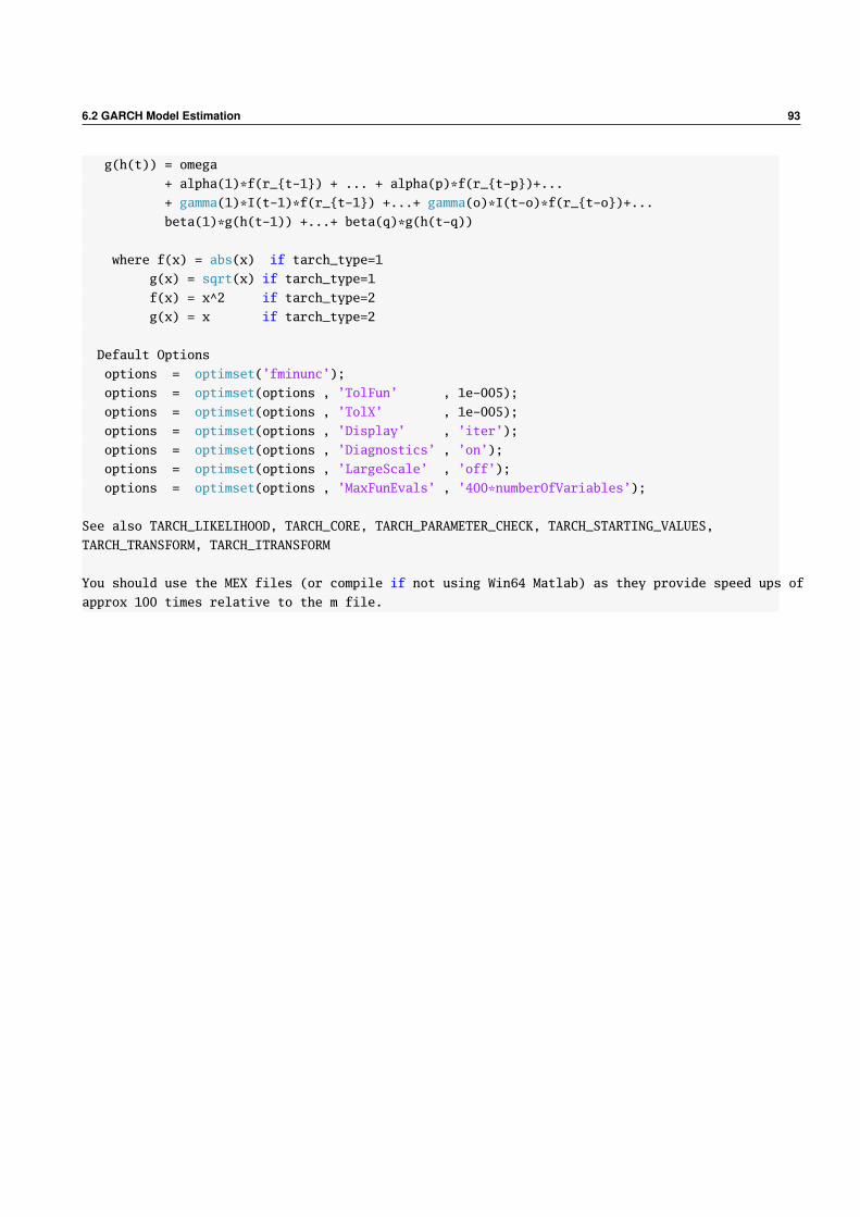
6.2 GARCH Model Estimation 93
g(h(t)) = omega
+ alpha(1)*f(r_t-1) + ... + alpha(p)*f(r_t-p)+...
+ gamma(1)*I(t-1)*f(r_t-1) +...+ gamma(o)*I(t-o)*f(r_t-o)+...
beta(1)*g(h(t-1)) +...+ beta(q)*g(h(t-q))
where f(x) = abs(x) if tarch_type=1
g(x) = sqrt(x) if tarch_type=1
f(x) = x^2 if tarch_type=2
g(x) = x if tarch_type=2
Default Options
options = optimset(’fminunc’);
options = optimset(options , ’TolFun’ , 1e-005);
options = optimset(options , ’TolX’ , 1e-005);
options = optimset(options , ’Display’ , ’iter’);
options = optimset(options , ’Diagnostics’ , ’on’);
options = optimset(options , ’LargeScale’ , ’off’);
options = optimset(options , ’MaxFunEvals’ , ’400*numberOfVariables’);
See also TARCH_LIKELIHOOD, TARCH_CORE, TARCH_PARAMETER_CHECK, TARCH_STARTING_VALUES,
TARCH_TRANSFORM, TARCH_ITRANSFORM
You should use the MEX files (or compile if not using Win64 Matlab) as they provide speed ups of
approx 100 times relative to the m file.
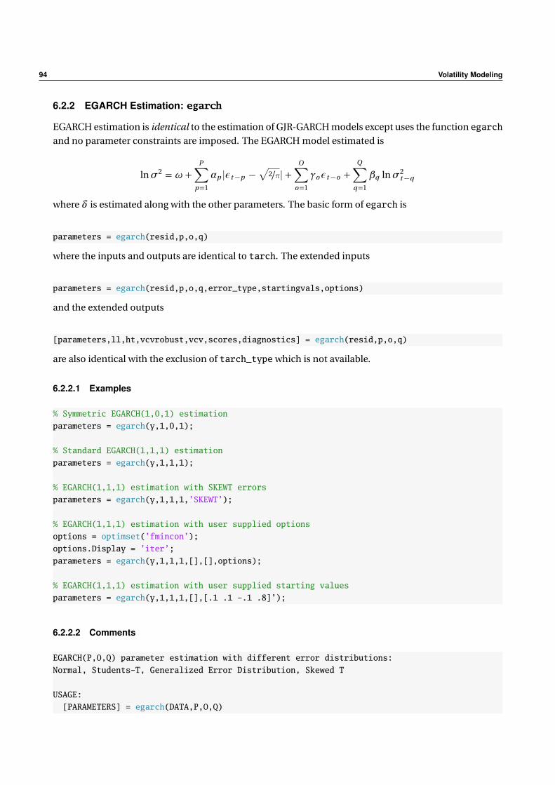
94 Volatility Modeling
6.2.2 EGARCH Estimation: egarch
EGARCH estimation is identical to the estimation of GJR-GARCH models except uses the function egarch
and no parameter constraints are imposed. The EGARCH model estimated is
lnσ2 = ω +P∑
p=1
αp |εt−p −√
2/π| +O∑
o=1
γoεt−o +Q∑
q=1
βq lnσ2t−q
where δ is estimated along with the other parameters. The basic form of egarch is
parameters = egarch(resid,p,o,q)
where the inputs and outputs are identical to tarch. The extended inputs
parameters = egarch(resid,p,o,q,error_type,startingvals,options)
and the extended outputs
[parameters,ll,ht,vcvrobust,vcv,scores,diagnostics] = egarch(resid,p,o,q)
are also identical with the exclusion of tarch_type which is not available.
6.2.2.1 Examples
% Symmetric EGARCH(1,0,1) estimation
parameters = egarch(y,1,0,1);
% Standard EGARCH(1,1,1) estimation
parameters = egarch(y,1,1,1);
% EGARCH(1,1,1) estimation with SKEWT errors
parameters = egarch(y,1,1,1,’SKEWT’);
% EGARCH(1,1,1) estimation with user supplied options
options = optimset(’fmincon’);
options.Display = ’iter’;
parameters = egarch(y,1,1,1,[],[],options);
% EGARCH(1,1,1) estimation with user supplied starting values
parameters = egarch(y,1,1,1,[],[.1 .1 -.1 .8]’);
6.2.2.2 Comments
EGARCH(P,O,Q) parameter estimation with different error distributions:
Normal, Students-T, Generalized Error Distribution, Skewed T
USAGE:
[PARAMETERS] = egarch(DATA,P,O,Q)
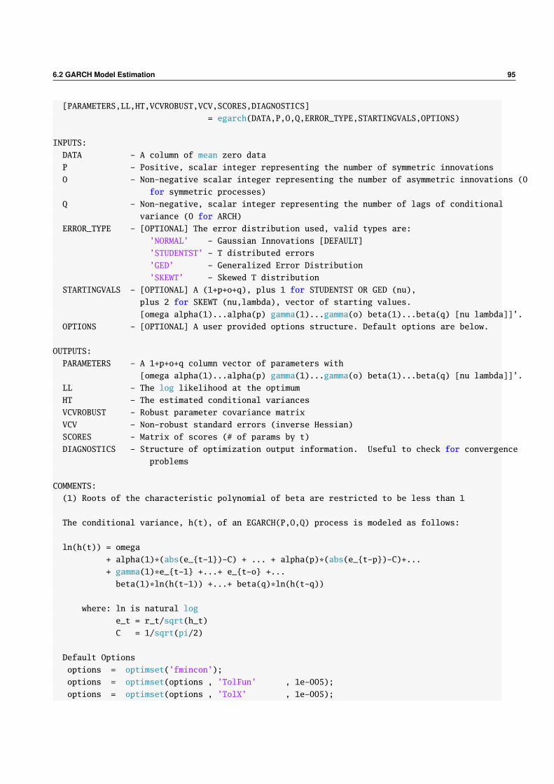
6.2 GARCH Model Estimation 95
[PARAMETERS,LL,HT,VCVROBUST,VCV,SCORES,DIAGNOSTICS]
= egarch(DATA,P,O,Q,ERROR_TYPE,STARTINGVALS,OPTIONS)
INPUTS:
DATA - A column of mean zero data
P - Positive, scalar integer representing the number of symmetric innovations
O - Non-negative scalar integer representing the number of asymmetric innovations (0
for symmetric processes)
Q - Non-negative, scalar integer representing the number of lags of conditional
variance (0 for ARCH)
ERROR_TYPE - [OPTIONAL] The error distribution used, valid types are:
’NORMAL’ - Gaussian Innovations [DEFAULT]
’STUDENTST’ - T distributed errors
’GED’ - Generalized Error Distribution
’SKEWT’ - Skewed T distribution
STARTINGVALS - [OPTIONAL] A (1+p+o+q), plus 1 for STUDENTST OR GED (nu),
plus 2 for SKEWT (nu,lambda), vector of starting values.
[omega alpha(1)...alpha(p) gamma(1)...gamma(o) beta(1)...beta(q) [nu lambda]]’.
OPTIONS - [OPTIONAL] A user provided options structure. Default options are below.
OUTPUTS:
PARAMETERS - A 1+p+o+q column vector of parameters with
[omega alpha(1)...alpha(p) gamma(1)...gamma(o) beta(1)...beta(q) [nu lambda]]’.
LL - The log likelihood at the optimum
HT - The estimated conditional variances
VCVROBUST - Robust parameter covariance matrix
VCV - Non-robust standard errors (inverse Hessian)
SCORES - Matrix of scores (# of params by t)
DIAGNOSTICS - Structure of optimization output information. Useful to check for convergence
problems
COMMENTS:
(1) Roots of the characteristic polynomial of beta are restricted to be less than 1
The conditional variance, h(t), of an EGARCH(P,O,Q) process is modeled as follows:
ln(h(t)) = omega
+ alpha(1)*(abs(e_t-1)-C) + ... + alpha(p)*(abs(e_t-p)-C)+...
+ gamma(1)*e_t-1 +...+ e_t-o +...
beta(1)*ln(h(t-1)) +...+ beta(q)*ln(h(t-q))
where: ln is natural log
e_t = r_t/sqrt(h_t)
C = 1/sqrt(pi/2)
Default Options
options = optimset(’fmincon’);
options = optimset(options , ’TolFun’ , 1e-005);
options = optimset(options , ’TolX’ , 1e-005);

96 Volatility Modeling
options = optimset(options , ’Display’ , ’iter’);
options = optimset(options , ’LargeScale’ , ’off’);
options = optimset(options , ’MaxFunEvals’ , 200*(2+p+q));
options = optimset(options , ’MaxSQPIter’ , 500);
options = optimset(options , ’Algorithm’ ,’active-set’);
See also EGARCH_LIKELIHOOD, EGARCH_CORE, EGARCH_PARAMETER_CHECK, EGARCH_STARTING_VALUES,
EGARCH_TRANSFORM, EGARCH_ITRANSFORM, EGARCH_NLCOM
You should use the MEX files (or compile if not using Win64 Matlab) as they provide speed ups of
approx 100 times relative to the m file
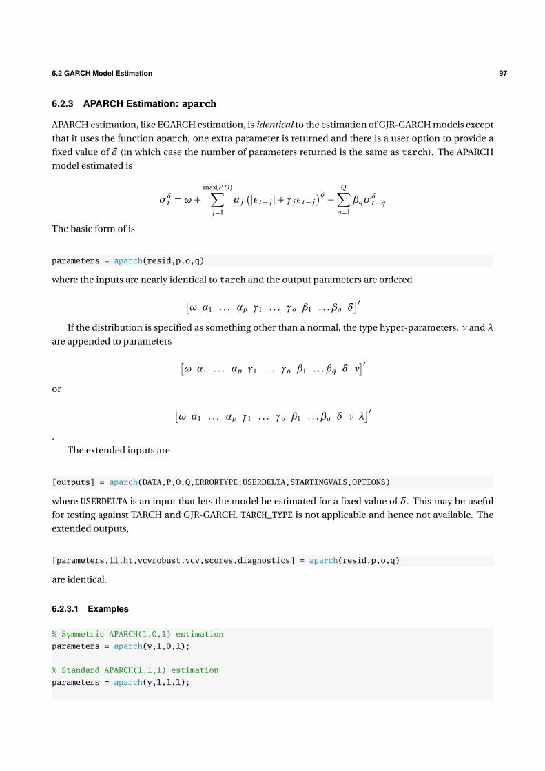
6.2 GARCH Model Estimation 97
6.2.3 APARCH Estimation: aparch
APARCH estimation, like EGARCH estimation, is identical to the estimation of GJR-GARCH models except
that it uses the function aparch, one extra parameter is returned and there is a user option to provide a
fixed value of δ (in which case the number of parameters returned is the same as tarch). The APARCH
model estimated is
σδt = ω +max(P,O )∑
j=1
α j(|εt− j | + γ jεt− j
)δ + Q∑q=1
βqσδt−q
The basic form of is
parameters = aparch(resid,p,o,q)
where the inputs are nearly identical to tarch and the output parameters are ordered
[ω α1 . . . αp γ1 . . . γo β1 . . .βq δ
]′If the distribution is specified as something other than a normal, the type hyper-parameters, ν and λ
are appended to parameters
[ω α1 . . . αp γ1 . . . γo β1 . . .βq δ ν
]′or
[ω α1 . . . αp γ1 . . . γo β1 . . .βq δ ν λ
]′.
The extended inputs are
[outputs] = aparch(DATA,P,O,Q,ERRORTYPE,USERDELTA,STARTINGVALS,OPTIONS)
where USERDELTA is an input that lets the model be estimated for a fixed value of δ. This may be useful
for testing against TARCH and GJR-GARCH. TARCH_TYPE is not applicable and hence not available. The
extended outputs,
[parameters,ll,ht,vcvrobust,vcv,scores,diagnostics] = aparch(resid,p,o,q)
are identical.
6.2.3.1 Examples
% Symmetric APARCH(1,0,1) estimation
parameters = aparch(y,1,0,1);
% Standard APARCH(1,1,1) estimation
parameters = aparch(y,1,1,1);
98 Volatility Modeling
% APARCH(1,1,1) estimation with SKEWT errors
parameters = aparch(y,1,1,1,’SKEWT’);
% APARCH(1,1,1) estimation with fixed delta of 1.5
parameters = aparch(y,1,1,1,[],1.5);
% APARCH(1,1,1) estimation with user supplied options
options = optimset(’fmincon’);
options.Display = ’iter’;
parameters = aparch(y,1,1,1,[],[],[],options);
% APARCH(1,1,1) estimation with user supplied starting values
parameters = aparch(y,1,1,1,[],[],[.1 .1 -.1 .8 1]’);
6.2.3.2 Comments
APARCH(P,O,Q) parameter estimation with different error distributions:
Normal, Students-T, Generalized Error Distribution, Skewed T
USAGE:
[PARAMETERS] = aparch(DATA,P,O,Q)
[PARAMETERS,LL,HT,VCVROBUST,VCV,SCORES,DIAGNOSTICS]
= aparch(DATA,P,O,Q,ERRORTYPE,USERDELTA,STARTINGVALS,OPTIONS)
INPUTS:
DATA - A column of mean zero data
P - Positive, scalar integer representing the number of symmetric innovations
O - Non-negative scalar integer representing the number of asymmetric innovations (0
for symmetric processes)
Q - Non-negative, scalar integer representing the number of lags of conditional
variance (0 for ARCH)
ERRORTYPE - [OPTIONAL] The error distribution used, valid types are:
’NORMAL’ - Gaussian Innovations [DEFAULT]
’STUDENTST’ - T distributed errors
’GED’ - Generalized Error Distribution
’SKEWT’ - Skewed T distribution
USERDELTA - [OPTIONAL] A scalar value between 0.3 and 4 to use for delta in the estimation.
When the user provides a fixed value for delta, the vector of PARAMETERS has
one less element. This is useful for testing an unrestricted APARCH against
TARCH or GJR-GARCH alternatives
STARTINGVALS - [OPTIONAL] A (1+p+o+q+1), plus 1 for STUDENTST OR GED (nu), plus 2 for SKEWT
(nu,lambda), vector of starting values.
[omega alpha(1)...alpha(p) gamma(1)...gamma(o) beta(1)...beta(q) delta [nu lambda]]’.
OPTIONS - [OPTIONAL] A user provided options structure. Default options are below.
OUTPUTS:
PARAMETERS - A 1+p+o+q+1 (+1 or 2) column vector of parameters with
[omega alpha(1)...alpha(p) gamma(1)...gamma(o) beta(1)...beta(q) delta [nu lambda]]’.
LL - The log likelihood at the optimum
6.2 GARCH Model Estimation 99
HT - The estimated conditional variances
VCVROBUST - Robust parameter covariance matrix
VCV - Non-robust standard errors (inverse Hessian)
SCORES - Matrix of scores (# of params by t)
DIAGNOSTICS - Structure of optimization output information. Useful to check for convergence
problems
COMMENTS:
The following (generally wrong) constraints are used:
(1) omega > 0
(2) alpha(i) >= 0 for i = 1,2,...,p
(3) 1<gamma<1 for i=1,...,o
(3) beta(i) >= 0 for i = 1,2,...,q
(4) delta>.3
(5) sum(alpha(i) + beta(k)) < 1 for i = 1,2,...p and k=1,2,...,q
(6) nu>2 of Students T and nu>1 for GED
(7) -.99<lambda<.99 for Skewed T
The conditional variance, h(t), of a APARCH(P,O,Q) process is modeled as follows:
h(t)^(delta/2) = omega
+ alpha(1)*(abs(r(t-1))+gamma(1)*r(t-1))^delta + ...
alpha(p)*(abs(r(t-p))+gamma(p)*r(t-p))^delta +
beta(1)*h(t-1)^(delta/2) +...+ beta(q)*h(t-q)^(delta/2)
Default Options
options = optimset(’fmincon’);
options = optimset(options , ’TolFun’ , 1e-005);
options = optimset(options , ’TolX’ , 1e-005);
options = optimset(options , ’Display’ , ’iter’);
options = optimset(options , ’Diagnostics’ , ’on’);
options = optimset(options , ’LargeScale’ , ’off’);
options = optimset(options , ’MaxFunEvals’ , ’400*numberOfVariables’);
See also APARCH_LIKELIHOOD, APARCH_CORE, APARCH_PARAMETER_CHECK, APARCH_STARTING_VALUES,
APARCH_TRANSFORM, APARCH_ITRANSFORM
You should use the MEX files (or compile if not using Win64 Matlab) as they provide speed ups of
approx 100 times relative to the m file
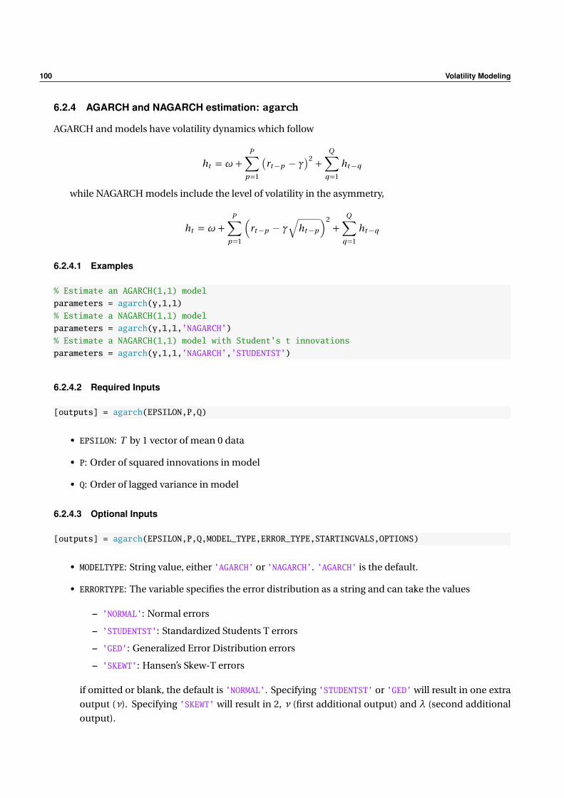
100 Volatility Modeling
6.2.4 AGARCH and NAGARCH estimation: agarch
AGARCH and models have volatility dynamics which follow
ht = ω +P∑
p=1
(rt−p − γ
)2 +Q∑
q=1
ht−q
while NAGARCH models include the level of volatility in the asymmetry,
ht = ω +P∑
p=1
(rt−p − γ
√ht−p
)2+
Q∑q=1
ht−q
6.2.4.1 Examples
% Estimate an AGARCH(1,1) model
parameters = agarch(y,1,1)
% Estimate a NAGARCH(1,1) model
parameters = agarch(y,1,1,’NAGARCH’)
% Estimate a NAGARCH(1,1) model with Student’s t innovations
parameters = agarch(y,1,1,’NAGARCH’,’STUDENTST’)
6.2.4.2 Required Inputs
[outputs] = agarch(EPSILON,P,Q)
• EPSILON: T by 1 vector of mean 0 data
• P: Order of squared innovations in model
• Q: Order of lagged variance in model
6.2.4.3 Optional Inputs
[outputs] = agarch(EPSILON,P,Q,MODEL_TYPE,ERROR_TYPE,STARTINGVALS,OPTIONS)
• MODELTYPE: String value, either ’AGARCH’ or ’NAGARCH’. ’AGARCH’ is the default.
• ERRORTYPE: The variable specifies the error distribution as a string and can take the values
– ’NORMAL’: Normal errors
– ’STUDENTST’: Standardized Students T errors
– ’GED’: Generalized Error Distribution errors
– ’SKEWT’: Hansen’s Skew-T errors
if omitted or blank, the default is ’NORMAL’. Specifying ’STUDENTST’ or ’GED’ will result in one extra
output (ν). Specifying ’SKEWT’ will result in 2, ν (first additional output) and λ (second additional
output).
6.2 GARCH Model Estimation 101
• STARTINGVALS: 2 + P + Q by 1 vector of starting values. If not provided, a grid search is performed
using common values.
• OPTIONS: Options structure for fminunc optimization.
6.2.4.4 Outputs
[PARAMETERS,LL,HT,VCVROBUST,VCV,SCORES,DIAGNOSTICS] = agarch(inputs)
• PARAMETERS: A 2+p+q vector of estimated parameters. If ERRORTYPE is ’STUDENTST’ or ’GED’, an addi-
tional parameter (ν) is returned. If ERRORTYPE is ’SKEWT’, two additional parameters will be returned,
ν (first additional output) and λ (second additional output).
• LL: Log-likelihood at the optimum.
• HT: T by 1 vector of fit conditional variances
• VCVROBUST: The Bollerslev-Wooldridge robust covariance matrix of the estimated parameters.
• VCV: The maximum likelihood covariance matrix (inverse Hessian) of the estimated parameters.
• SCORES: A T by number of parameters matrix of scores of the parameters. Used in some diagnostic
tests.
• DIAGNOSTICS: A structure that contains information about the status of the optimizer. Useful for
checking if there are convergence problems.
6.2.4.5 Comments
AGARCH(P,Q) and NAGARCH(P,Q) with different error distributions:
Normal, Students-T, Generalized Error Distribution, Skewed T
USAGE:
[PARAMETERS] = agarch(EPSILON,P,Q)
[PARAMETERS,LL,HT,VCVROBUST,VCV,SCORES,DIAGNOSTICS]
= agarch(EPSILON,P,Q,MODEL_TYPE,ERROR_TYPE,STARTINGVALS,OPTIONS)
INPUTS:
EPSILON - A column of mean zero data
P - Positive, scalar integer representing the number of symmetric innovations
Q - Non-negative, scalar integer representing the number of lags of conditional
variance (0 for ARCH-type model)
MODEL_TYPE - [OPTIONAL] The type of variance process, either
’AGARCH’ - Asymmetric GARCH, Engle (1990) [DEFAULT]
’NAGARCH’ - Nonlinear Asymmetric GARCH, Engle & Ng (1993)
ERROR_TYPE - [OPTIONAL] The error distribution used, valid types are:
’NORMAL’ - Gaussian Innovations [DEFAULT]
’STUDENTST’ - T distributed errors
’GED’ - Generalized Error Distribution
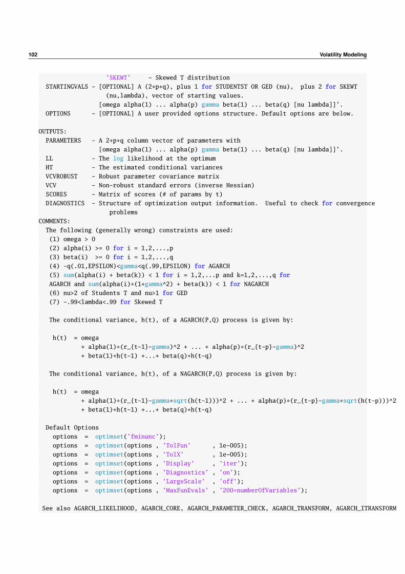
102 Volatility Modeling
’SKEWT’ - Skewed T distribution
STARTINGVALS - [OPTIONAL] A (2+p+q), plus 1 for STUDENTST OR GED (nu), plus 2 for SKEWT
(nu,lambda), vector of starting values.
[omega alpha(1) ... alpha(p) gamma beta(1) ... beta(q) [nu lambda]]’.
OPTIONS - [OPTIONAL] A user provided options structure. Default options are below.
OUTPUTS:
PARAMETERS - A 2+p+q column vector of parameters with
[omega alpha(1) ... alpha(p) gamma beta(1) ... beta(q) [nu lambda]]’.
LL - The log likelihood at the optimum
HT - The estimated conditional variances
VCVROBUST - Robust parameter covariance matrix
VCV - Non-robust standard errors (inverse Hessian)
SCORES - Matrix of scores (# of params by t)
DIAGNOSTICS - Structure of optimization output information. Useful to check for convergence
problems
COMMENTS:
The following (generally wrong) constraints are used:
(1) omega > 0
(2) alpha(i) >= 0 for i = 1,2,...,p
(3) beta(i) >= 0 for i = 1,2,...,q
(4) -q(.01,EPSILON)<gamma<q(.99,EPSILON) for AGARCH
(5) sum(alpha(i) + beta(k)) < 1 for i = 1,2,...p and k=1,2,...,q for
AGARCH and sum(alpha(i)*(1+gamma^2) + beta(k)) < 1 for NAGARCH
(6) nu>2 of Students T and nu>1 for GED
(7) -.99<lambda<.99 for Skewed T
The conditional variance, h(t), of a AGARCH(P,Q) process is given by:
h(t) = omega
+ alpha(1)*(r_t-1-gamma)^2 + ... + alpha(p)*(r_t-p-gamma)^2
+ beta(1)*h(t-1) +...+ beta(q)*h(t-q)
The conditional variance, h(t), of a NAGARCH(P,Q) process is given by:
h(t) = omega
+ alpha(1)*(r_t-1-gamma*sqrt(h(t-1)))^2 + ... + alpha(p)*(r_t-p-gamma*sqrt(h(t-p)))^2
+ beta(1)*h(t-1) +...+ beta(q)*h(t-q)
Default Options
options = optimset(’fminunc’);
options = optimset(options , ’TolFun’ , 1e-005);
options = optimset(options , ’TolX’ , 1e-005);
options = optimset(options , ’Display’ , ’iter’);
options = optimset(options , ’Diagnostics’ , ’on’);
options = optimset(options , ’LargeScale’ , ’off’);
options = optimset(options , ’MaxFunEvals’ , ’200*numberOfVariables’);
See also AGARCH_LIKELIHOOD, AGARCH_CORE, AGARCH_PARAMETER_CHECK, AGARCH_TRANSFORM, AGARCH_ITRANSFORM

6.2 GARCH Model Estimation 103
You should use the MEX files (or compile if not using Win64 Matlab) as they provide speed ups of
approx 10 times relative to the m file
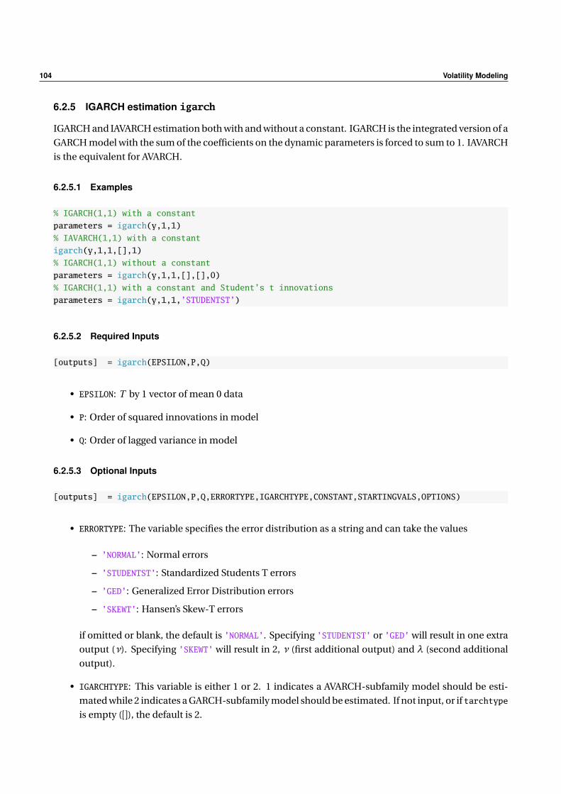
104 Volatility Modeling
6.2.5 IGARCH estimation igarch
IGARCH and IAVARCH estimation both with and without a constant. IGARCH is the integrated version of a
GARCH model with the sum of the coefficients on the dynamic parameters is forced to sum to 1. IAVARCH
is the equivalent for AVARCH.
6.2.5.1 Examples
% IGARCH(1,1) with a constant
parameters = igarch(y,1,1)
% IAVARCH(1,1) with a constant
igarch(y,1,1,[],1)
% IGARCH(1,1) without a constant
parameters = igarch(y,1,1,[],[],0)
% IGARCH(1,1) with a constant and Student’s t innovations
parameters = igarch(y,1,1,’STUDENTST’)
6.2.5.2 Required Inputs
[outputs] = igarch(EPSILON,P,Q)
• EPSILON: T by 1 vector of mean 0 data
• P: Order of squared innovations in model
• Q: Order of lagged variance in model
6.2.5.3 Optional Inputs
[outputs] = igarch(EPSILON,P,Q,ERRORTYPE,IGARCHTYPE,CONSTANT,STARTINGVALS,OPTIONS)
• ERRORTYPE: The variable specifies the error distribution as a string and can take the values
– ’NORMAL’: Normal errors
– ’STUDENTST’: Standardized Students T errors
– ’GED’: Generalized Error Distribution errors
– ’SKEWT’: Hansen’s Skew-T errors
if omitted or blank, the default is ’NORMAL’. Specifying ’STUDENTST’ or ’GED’ will result in one extra
output (ν). Specifying ’SKEWT’ will result in 2, ν (first additional output) and λ (second additional
output).
• IGARCHTYPE: This variable is either 1 or 2. 1 indicates a AVARCH-subfamily model should be esti-
mated while 2 indicates a GARCH-subfamily model should be estimated. If not input, or if tarchtype
is empty ([]), the default is 2.

6.2 GARCH Model Estimation 105
• CONSTANT: Logical value indicating whether a constant should be included in the model. The default
is 1.
• STARTINGVALS: A CONSTANT+P+Q-1 vector of starting values. If ERRORTYPE is ’STUDENTST’ or ’GED’, an
additional starting value is needed. IfERRORTYPE is’SKEWT’ two additional starting values are needed.
If startingvals is empty or omitted, a simple grid search is used for starting values.
• OPTIONS: A valid fminunc options structure. The defaults are listed in the comments. This options is
useful for preventing output from being displayed if calling the routine many times.
6.2.5.4 Outputs
[PARAMETERS,LL,HT,VCVROBUST,VCV,SCORES,DIAGNOSTICS] = igarch(inputs)
• PARAMETERS: A CONSTANT+P+Q-1 vector of estimated parameters. If ERRORTYPE is ’STUDENTST’ or ’GED’,
an additional parameter (ν) is returned. If ERRORTYPE is ’SKEWT’, two additional parameters will be
returned, ν (first additional output) and λ (second additional output).
• LL: Log-likelihood at the optimum.
• HT: T by 1 vector of fit conditional variances
• VCVROBUST: The Bollerslev-Wooldridge robust covariance matrix of the estimated parameters.
• VCV: The maximum likelihood covariance matrix (inverse Hessian) of the estimated parameters.
• SCORES: A T by number of parameters matrix of scores of the parameters. Used in some diagnostic
tests.
• DIAGNOSTICS: A structure that contains information about the status of the optimizer. Useful for
checking if there are convergence problems.
6.2.5.5 Comments
IGARCH(P,Q) parameter estimation with different error distributions
Normal, Students-T, Generalized Error Distribution, Skewed T
Estimation of IGARCH models if IGARCHTYPE=2
Estimation of IAVARCH if IGARCHTYPE=1
USAGE:
[PARAMETERS] = igarch(EPSILON,P,O,Q)
[PARAMETERS,LL,HT,VCVROBUST,VCV,SCORES,DIAGNOSTICS]
= igarch(EPSILON,P,Q,ERRORTYPE,IGARCHTYPE,CONSTANT,STARTINGVALS,OPTIONS)
INPUTS:
EPSILON - A column of mean zero data
P - Positive, scalar integer representing the number of innovations
Q - Positive, scalar integer representing the number of lags of conditional variance
ERRORTYPE - [OPTIONAL] The error distribution used, valid types are:
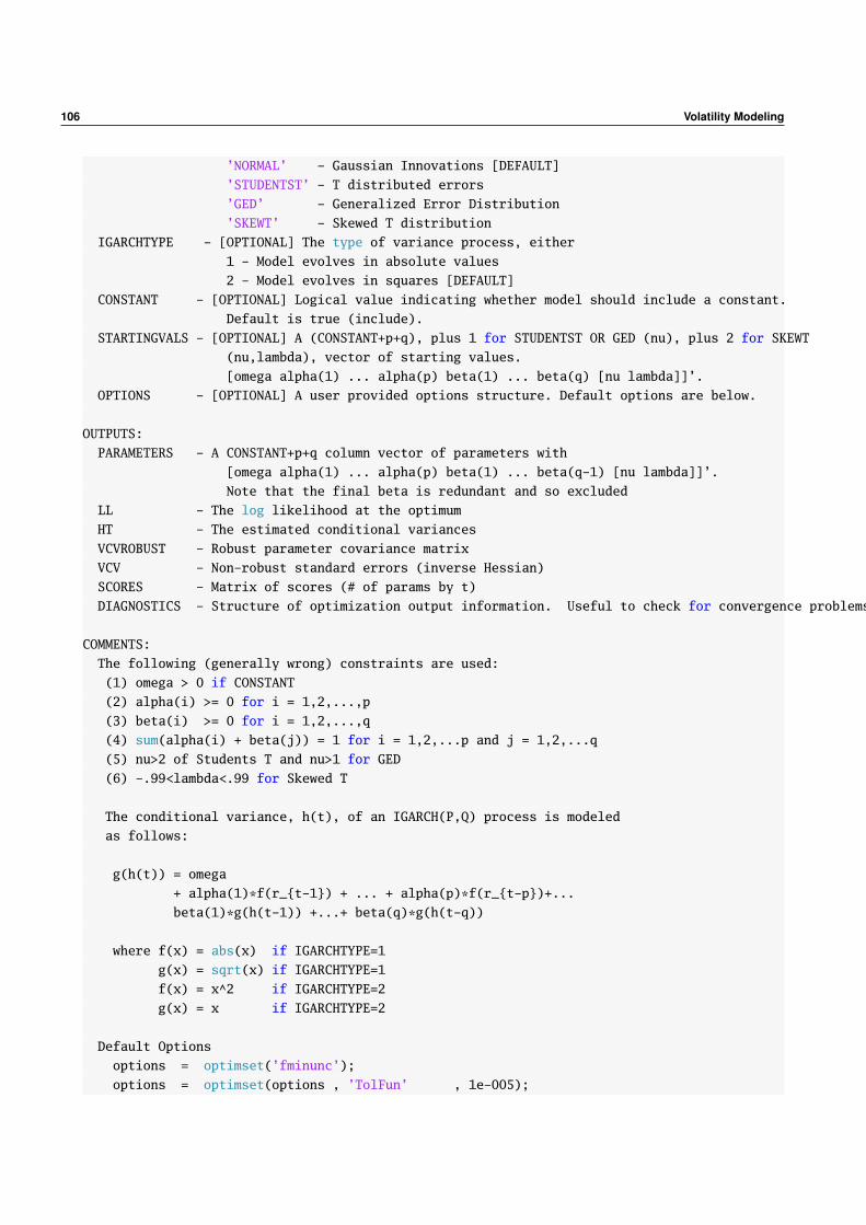
106 Volatility Modeling
’NORMAL’ - Gaussian Innovations [DEFAULT]
’STUDENTST’ - T distributed errors
’GED’ - Generalized Error Distribution
’SKEWT’ - Skewed T distribution
IGARCHTYPE - [OPTIONAL] The type of variance process, either
1 - Model evolves in absolute values
2 - Model evolves in squares [DEFAULT]
CONSTANT - [OPTIONAL] Logical value indicating whether model should include a constant.
Default is true (include).
STARTINGVALS - [OPTIONAL] A (CONSTANT+p+q), plus 1 for STUDENTST OR GED (nu), plus 2 for SKEWT
(nu,lambda), vector of starting values.
[omega alpha(1) ... alpha(p) beta(1) ... beta(q) [nu lambda]]’.
OPTIONS - [OPTIONAL] A user provided options structure. Default options are below.
OUTPUTS:
PARAMETERS - A CONSTANT+p+q column vector of parameters with
[omega alpha(1) ... alpha(p) beta(1) ... beta(q-1) [nu lambda]]’.
Note that the final beta is redundant and so excluded
LL - The log likelihood at the optimum
HT - The estimated conditional variances
VCVROBUST - Robust parameter covariance matrix
VCV - Non-robust standard errors (inverse Hessian)
SCORES - Matrix of scores (# of params by t)
DIAGNOSTICS - Structure of optimization output information. Useful to check for convergence problems
COMMENTS:
The following (generally wrong) constraints are used:
(1) omega > 0 if CONSTANT
(2) alpha(i) >= 0 for i = 1,2,...,p
(3) beta(i) >= 0 for i = 1,2,...,q
(4) sum(alpha(i) + beta(j)) = 1 for i = 1,2,...p and j = 1,2,...q
(5) nu>2 of Students T and nu>1 for GED
(6) -.99<lambda<.99 for Skewed T
The conditional variance, h(t), of an IGARCH(P,Q) process is modeled
as follows:
g(h(t)) = omega
+ alpha(1)*f(r_t-1) + ... + alpha(p)*f(r_t-p)+...
beta(1)*g(h(t-1)) +...+ beta(q)*g(h(t-q))
where f(x) = abs(x) if IGARCHTYPE=1
g(x) = sqrt(x) if IGARCHTYPE=1
f(x) = x^2 if IGARCHTYPE=2
g(x) = x if IGARCHTYPE=2
Default Options
options = optimset(’fminunc’);
options = optimset(options , ’TolFun’ , 1e-005);
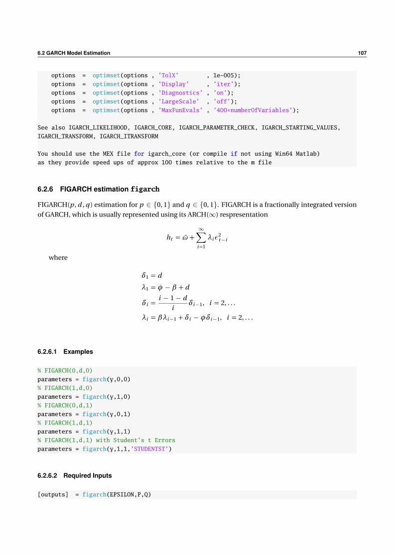
6.2 GARCH Model Estimation 107
options = optimset(options , ’TolX’ , 1e-005);
options = optimset(options , ’Display’ , ’iter’);
options = optimset(options , ’Diagnostics’ , ’on’);
options = optimset(options , ’LargeScale’ , ’off’);
options = optimset(options , ’MaxFunEvals’ , ’400*numberOfVariables’);
See also IGARCH_LIKELIHOOD, IGARCH_CORE, IGARCH_PARAMETER_CHECK, IGARCH_STARTING_VALUES,
IGARCH_TRANSFORM, IGARCH_ITRANSFORM
You should use the MEX file for igarch_core (or compile if not using Win64 Matlab)
as they provide speed ups of approx 100 times relative to the m file
6.2.6 FIGARCH estimation figarch
FIGARCH(p , d , q ) estimation for p ∈ 0, 1 and q ∈ 0, 1. FIGARCH is a fractionally integrated version
of GARCH, which is usually represented using its ARCH(∞) respresentation
ht = ω +∞∑
i=1
λiε2t−i
where
δ1 = d
λ1 = φ − β + d
δi =i − 1− d
iδi−1, i = 2, . . .
λi = βλi−1 + δi − φδi−1, i = 2, . . .
6.2.6.1 Examples
% FIGARCH(0,d,0)
parameters = figarch(y,0,0)
% FIGARCH(1,d,0)
parameters = figarch(y,1,0)
% FIGARCH(0,d,1)
parameters = figarch(y,0,1)
% FIGARCH(1,d,1)
parameters = figarch(y,1,1)
% FIGARCH(1,d,1) with Student’s t Errors
parameters = figarch(y,1,1,’STUDENTST’)
6.2.6.2 Required Inputs
[outputs] = figarch(EPSILON,P,Q)
108 Volatility Modeling
• EPSILON: T by 1 vector of mean 0 data
• P: Order of the short memory autoregressive process. Must be 0 or 1.
• Q: Order of the moving average process. Must be 0 or 1.
6.2.6.3 Optional Inputs
[outputs] = figarch(EPSILON,P,Q,ERRORTYPE,TRUNCLAG,STARTINGVALS,OPTIONS)
• ERRORTYPE: The variable specifies the error distribution as a string and can take the values
– ’NORMAL’: Normal errors
– ’STUDENTST’: Standardized Students T errors
– ’GED’: Generalized Error Distribution errors
– ’SKEWT’: Hansen’s Skew-T errors
if omitted or blank, the default is ’NORMAL’. Specifying ’STUDENTST’ or ’GED’ will result in one extra
output (ν). Specifying ’SKEWT’ will result in 2, ν (first additional output) and λ (second additional
output).
• TRUNCLAG: Truncation point for ARCH(∞) representation.
• STARTINGVALS: A 2+P+Q vector of starting values. If ERRORTYPE is ’STUDENTST’ or ’GED’, an addi-
tional starting value is needed. If ERRORTYPE is ’SKEWT’ two additional starting values are needed.
If startingvals is empty or omitted, a simple grid search is used for starting values.
• OPTIONS: A valid fminunc options structure. The defaults are listed in the comments. This options is
useful for preventing output from being displayed if calling the routine many times.
6.2.6.4 Outputs
[PARAMETERS,LL,HT,VCVROBUST,VCV,SCORES,DIAGNOSTICS] = figarch(inputs)
• PARAMETERS: A 2+P+Q vector of estimated parameters. If ERRORTYPE is ’STUDENTST’ or ’GED’, an addi-
tional parameter (ν) is returned. If ERRORTYPE is ’SKEWT’, two additional parameters will be returned,
ν (first additional output) and λ (second additional output).
• LL: Log-likelihood at the optimum.
• HT: T by 1 vector of fit conditional variances
• VCVROBUST: The Bollerslev-Wooldridge robust covariance matrix of the estimated parameters.
• VCV: The maximum likelihood covariance matrix (inverse Hessian) of the estimated parameters.
• SCORES: A T by number of parameters matrix of scores of the parameters. Used in some diagnostic
tests.
• DIAGNOSTICS: A structure that contains information about the status of the optimizer. Useful for
checking if there are convergence problems.
6.2 GARCH Model Estimation 109
6.2.6.5 Comments
FIGARCH(Q,D,P) parameter estimation for P=0,1 and Q=0,1 with different error distributions:
Normal, Students-T, Generalized Error Distribution, Skewed T
USAGE:
[PARAMETERS] = figarch(EPSILON,P,Q)
[PARAMETERS,LL,HT,VCVROBUST,VCV,SCORES,DIAGNOSTICS]
= figarch(EPSILON,P,Q,ERRORTYPE,STARTINGVALS,OPTIONS)
INPUTS:
EPSILON - T by 1 Column vector of mean zero residuals
P - 0 or 1 indicating whether the autoregressive term is present in the model (phi)
Q - 0 or 1 indicating whether the moving average term is present in the model (beta)
ERRORTYPE - [OPTIONAL] The error distribution used, valid types are:
’NORMAL’ - Gaussian Innovations [DEFAULT]
’STUDENTST’ - T distributed errors
’GED’ - Generalized Error Distribution
’SKEWT’ - Skewed T distribution
TRUNCLAG - [OPTIONAL] Number of weights to compute in ARCH(oo) representation.
Default is 1000.
STARTINGVALS - [OPTIONAL] A (2+p+q), plus 1 for STUDENTST OR GED (nu), plus 2 for SKEWT
(nu,lambda), vector of starting values. [omega phi d beta [nu lambda]]’.
If
not provided, FIGARCH_STARTING_VALUES attempts to find reasonable values.
OPTIONS - [OPTIONAL] A user provided options structure. Default options are below.
OUTPUTS:
PARAMETERS - A 2+p+q column vector of parameters with [omega phi d beta [nu lambda]]’.
LL - The log likelihood at the optimum
HT - The estimated conditional variances
VCVROBUST - Robust parameter covariance matrix
VCV - Non-robust standard errors (inverse Hessian)
SCORES - Matrix of scores (# of params by t)
DIAGNOSTICS - Structure of optimization output information. Useful to check for convergence
problems .
COMMENTS:
The following (generally wrong) constraints are used:
(1) omega > 0
(2) 0<= d <= 1
(3) 0 <= phi <= (1-d)/2
(3) 0 <= beta <= d + phi
(5) nu>2 of Students T and nu>1 for GED
(6) -.99<lambda<.99 for Skewed T
The conditional variance, h(t), of a FIGARCH(1,d,1) process is modeled as follows:
h(t) = omega + [1-beta L - phi L (1-L)^d] epsilon(t)^2 + beta * h(t-1)
where L is the lag operator which is estimated using an ARCH(oo) representation,
110 Volatility Modeling
h(t) = omega + sum(lambda(i) * epsilon(t-1)^2)
where lambda(i) is a function of the fractional differencing parameter, phi and beta.
Default Options
options = optimset(’fminunc’);
options = optimset(options , ’TolFun’ , 1e-005);
options = optimset(options , ’TolX’ , 1e-005);
options = optimset(options , ’Display’ , ’iter’);
options = optimset(options , ’Diagnostics’ , ’on’);
options = optimset(options , ’LargeScale’ , ’off’);
options = optimset(options , ’MaxFunEvals’ , ’400*numberOfVariables’);
See also TARCH, APARCH, EGARCH, AGARCH, FIGARCH_LIKELIHOOD, FIGARCH_PARAMETER_CHECK,
FIGARCH_WEIGHTS FIGARCH_STARTING_VALUES, FIGARCH_TRANSFORM, FIGARCH_ITRANSFORM
Chapter 7
Density Estimation
7.1 Kernel Density Estimation: pltdens
Kernel density estimation is a useful tool to visualize the distribution of returns which would having to
make strong parametric assumptions. Let yt Tt=1 be a set of i.i.d. data. The kernel density around a point
x is defined
f (x ) =t∑
t=1
K
(yt − x
h
)where h is the bandwidth, a parameter that controls the width of the window. pltdens supports a number
of Kernels
• Gaussian
K (z ) =1√2π
exp(−z 2/2)
• Epanechnikov
K (z ) =
34 (1− z 2) −1 ≤ z ≤ 1
0 otherwise
• Quartic (Biweight)
K (z ) =
1516 (1− z 2)2 −1 ≤ z ≤ 1
0 otherwise
• Triweight
K (z ) =
3532 (1− z 2)3 −1 ≤ z ≤ 1
0 otherwise
For i.i.d. data Silverman’s bandwidth, 1.06σ2T −15 has good properties and is used by default. The function
can be used two ways. The first is to produce the kernel density plot and is simply
pltdens(y)
The second computes the weights but does not produce a plot
112 Density Estimation
[h,f,y] = pltdens(y);
Data on the S&P 500 were used to produce 3 kernel densities, one with Silverman’s BW, on over-smoothed
(h large) and one under-smoothed (h small). The results of this code is contained in figure 9.1.
[h,f,y] = pltdens(SP500);
disp(h)
[hover,fover,yover] = pltdens(SP500,.01);
[hunder,funder,yunder] = pltdens(SP500,.0001);
fig = figure(1);
clf
set(fig,’PaperOrientation’,’landscape’,’PaperSize’,[11 8.5],...
’InvertHardCopy’,’off’,’PaperPositionMode’,’auto’,...
’Position’,[117 158 957 764],’Color’,[1 1 1]);
hfig = plot(y,f,yover,fover,yunder,funder);
axis tight
for i=1:3;set(hfig(i),’LineWidth’,2);end
legend(’Silvermann’,’Over smoothed’,’Under smoothed’)
set(gca,’FontSize’,14)
h =
.0027
7.1.0.1 Examples
% Produce a kernel plot
pltdens(y)
% Compute weights but do not produce a plot
[h,f,y] = pltdens(y);
% Produce the plot manually
plot(y,f)
% Specify a custom bandwidth
pltdens(y,3);
7.1.0.2 Comments
PURPOSE: Draw a nonparametric density estimate.
--------------------------------------------------
USAGE: [h,f,y] = pltdens(x,h,p,kernel)
or pltdens(x) which uses gaussian kernel default
where:
x is a vector
h is the kernel bandwidth
default=1.06 * std(x) * n^(-1/5); Silverman page 45
p is 1 if the density is 0 for negative values

7.1 Kernel Density Estimation: pltdens 113
−0.1 −0.08 −0.06 −0.04 −0.02 0 0.02 0.04 0.06 0.080
5
10
15
20
25
30
35
40
45
SilvermannOver smoothedUnder smoothed
Figure 7.1: A plot with kernel densities using Silverman’s BW and over- and under- smoothed.
k is the kernel type:
=1 Gaussian (default)
=2 Epanechnikov
=3 Biweight
=4 Triangular
A jittered plot of the

114 Density Estimation
observations is shown below the density.
--------------------------------------------------
RETURNS:
h = the interval used
f = the density
y = the domain of support
plot(y,f) will produce a plot of the density
--------------------------------------------------
SEE ALSO hist, histo
--------------------------------------------------
7.2 Distributional Fit Testing 115
7.2 Distributional Fit Testing
7.2.1 Jarque-Bera Test: jarquebera
Jarque-Bera test for normality, defined as
(T − K )(
sk 2
6+(κ− 3)2
24
)where sk is the sample skewness and κ is the sample kurtosis.
7.2.1.1 Examples
% Jarque-Bera test on normal data
x = randn(100,1);
[statistic, pval] = jarquebera(x);
% Jarque-Bera test on regression errors
% where there were 4 regressors (4 mean parameters + 1 variance)
y=randn(100,1);x = randn(100,4); e = y - x*(x
[statistic, pval] = jarquebera(e, 5)
7.2.1.2 Required Inputs
[outputs] = jarquebera(DATA)
• DATA: T by 1 vector of data to be tested.
7.2.1.3 Optional Inputs
[outputs] = jarquebera(DATA,K,ALPHA)
• K: Degree of freedom adjustment. Default is 2.
• ALPHA: Size of the test to use. Default is 5%.
7.2.1.4 Outputs
[STATISTIC,PVAL,H] = jarquebera(inputs)
• STATISTIC: Jarque-Bera test statistic.
• PVAL: P-value evaluated using the asymptotic χ22 distribution.
• H: Logical indicating whether the test rejects at ALPHA.
116 Density Estimation
7.2.1.5 Comments
Computes the Jarque-Bera test for normality using the skewness and kurtosis to determine if a
distribution is normal.
USAGE:
[STATISTIC] = jarquebera(DATA)
[STATISTIC,PVAL,H] = jarquebera(DATA,K,ALPHA)
INPUTS:
DATA - A set of data to be tested for deviations from normality
K - [OPTIONAL] The number of dependant variables if any used in constructing the errors
(if omitted K=2)
ALPHA - [OPTIONAL] The level of the test used for the null of normality. Default is .05
OUTPUTS:
STATISTIC - A scalar representing the statistic
PVAL - A scalar pval of the null
H - A hypothesis dummy (0 for fail to reject the null of normality, 1 otherwise)
COMMENTS:
The data entered can be mean 0 or not. In either case the sample mean is subtracted and the
data are standardized by the sample standard deviation before computing the statistic .
EXAMPLES:
J-B test on normal data
x = randn(100,1);
[statistic, pval] = jarquebeta(x);
J-B test on regression errors where there were 4 regressors (4 mean parameters + 1 variance)
x = randn(100,1);
[statistic, pval] = jarquebeta(x, 5)

7.2 Distributional Fit Testing 117
7.2.2 Kolmogorov-Smirnov Test: kolmogorov
Kolmogorov-Smirnov test for correct unconditional distribution.
7.2.2.1 Examples
% Test data for uniformity
stat = kolmogorov(x)
% Test standard normal data
[stat,pval] = kolmogorov(x,[],’normcdf’)
% Test normal mean 1, standard deviation 2 data
[stat,pval] = kolmogorov(x,[],’normcdf’,1,2)
7.2.2.2 Required Inputs
[outputs] = kolmogorov(X)
• X: Data to be tested. X should have been transformed such that it is uniform (under the hypothesized
distribution).
7.2.2.3 Optional Inputs
[outputs] = kolmogorov(X,ALPHA,DIST,VARARGIN)
• ALPHA: Size of the test to use. Default is 5%.
• DIST: A string or function handle containing the name of a CDF to use to transform X to be uniform
(under the hypothesized distribution).
• VARARGIN: Optional arguments needed by DIST.
7.2.2.4 Outputs
[STAT,PVAL,H] = kolmogorov(inputs)
• STATISTIC: Kolmogorov-Smirnov test statistic.
• PVAL: P-value evaluated using a Monte Carlo distribution.
• H: Logical indicating whether the test rejects at ALPHA.
118 Density Estimation
7.2.2.5 Comments
Performs a Kolmogorov-Smirnov test that the data are from a specified distribution
USAGE:
[STAT,PVAL,H] = kolmogorov(X,ALPHA,DIST,VARARGIN)
INPUTS:
X - A set of random variable to be tested for distributional correctness
ALPHA - [OPTIONAL] The size for the test or use for computing H. 0.05 if not entered or
empty.
DIST - [OPTIONAL] A char string of the name of the CDF, i.e. ’normcdf’ for the normal,
’stdtcdf’ for standardized Student’s T, etc. If not provided or empty, data are
assumed to have a uniform distribution (i.e. that data have already been fed
through a probability integral transform)
VARARGIN - [OPTIONAL] Arguments passed to the CDF, such as the mean and variance for a normal
or a d.f. for T. The VARARGIN should be such that DIST(X,VARARGIN) is a valid
function with the correct inputs.
OUTPUTS:
STAT - The KS statistic
PVAL - The asymptotic probability of significance
H - 1 for reject the null that the distribution is correct, using the size provided (or
.05 if not), 0 otherwise
EXAMPLES:
Test data for uniformity
stat = kolmogorov(x);
Test standard normal data
[stat,pval] = kolmogorov(x,[],’normcdf’);
Test normal mean 1, standard deviation 2 data
[stat,pval] = kolmogorov(x,[],’normcdf’,1,2);
COMMENTS:
See also BERKOWITZ
7.2 Distributional Fit Testing 119
7.2.3 Berkowitz Test: berkowitz
Berkowitz (2001) test for correct fit in conditional density models.
7.2.3.1 Examples
% Test uniform data from a TS model
stat = berkowitz(x);
% Test standard normal data from a TS model
[stat,pval] = berkowitz(x,’TS’,[],’normcdf’);
% Test normal mean 1, standard deviation 2 data from a TS model
[stat,pval] = berkowitz(x,’TS’,[],’normcdf’,1,2);
7.2.3.2 Required Inputs
[outputs] = berkowitz(X)
• X: Data to be tested. X should have been transformed such that it is uniform (under the hypothesized
distribution).
7.2.3.3 Optional Inputs
[outputs] = berkowitz(X,TYPE,ALPHA,DIST,VARARGIN)
• TYPE: String either ’TS’ or ’CS’. Determines whether the test statistics looks at the AR(1) coefficient
(’TS’ does, ’CS’ does not). Default is ’TS’.
• ALPHA: Size of the test to use. Default is 5%.
• DIST: A string or function handle containing the name of a CDF to use to transform X to be uniform
(under the hypothesized distribution).
• VARARGIN: Optional arguments needed by DIST.
7.2.3.4 Outputs
[STAT,PVAL,H] = berkowitz(inputs)
• STATISTIC: Berkowitz test statistic.
• PVAL: P-value evaluated using the asymptotic χ2q distribution where q = 2 or q = 3, depending on
TYPE.
• H: Logical indicating whether the test rejects at ALPHA.
120 Density Estimation
7.2.3.5 Comments
Performs a Kolmogorov-Smirnov-like test using the Berkowitz transformation to a univariate normal
that the data are from a specified distribution.
USAGE:
[STAT,PVAL,H] = berkowitz(X,TYPE,ALPHA,DIST,VARARGIN)
INPUTS:
X - A set of random variable to be tested for distributional correctness
TYPE - [OPTIONAL] A char string, either ’CS’ if the data are cross-sectional or ’TS’ for
time series. The TS checks for autocorrelation in the prob integral transforms
while the CS does not. ’TS’ is the default value.
ALPHA - [OPTIONAL] The size for the test or use for computing H. 0.05 if not entered or
empty.
DIST - [OPTIONAL] A char string of the name of the CDF of X, i.e. ’normcdf’ for the normal,
’stdtcdf’ for standardized Studnet’s T, etc. If not provided or empty, data are
assumed to have a uniform distribution (i.e. that data have already been fed
through a probability integral transform)
VARARGIN - [OPTIONAL] Arguments passed to the CDF, such as the mean and variance for a normal
or a d.f. for T. The VARARGIN should be such that DIST(X,VARARGIN) is a valid
function with the correct inputs.
OUTPUTS:
STAT - The Berkowitz statistic computed as a likelihood ratio of normals
PVAL - The asymptotic probability of significance
H - 1 for reject the null that the distribution is correct using the size provided (or
.05 if not), 0 otherwise
EXAMPLES:
Test uniform data from a TS model
stat = berkowitz(x);
Test standard normal data from a TS model
[stat,pval] = berkowitz(x,’TS’,[],’normcdf’);
Test normal mean 1, standard deviation 2 data from a TS model
[stat,pval] = berkowitz(x,’TS’,[],’normcdf’,1,2);
COMMENTS:
See also KOLMOGOROV
Chapter 8
Bootstrap and Multiple Hypothesis Tests
8.1 Bootstraps
8.1.1 Block Bootstrap: block_bootstrap
8.1.1.1 Examples
% 1000 block bootstraps with a block size of 12
bsData = block_bootstrap(data, 1000, 12)
% Vector block bootstraps with a block size of 12
[t,k] = size(data,1);
bsIndex = block_bootstrap(1:t, 1000, 12)
for i=1:1000
bsData = data(bsIndex(:,i),:);
% Statistics here
end
8.1.1.2 Required Inputs
[BSDATA, INDICES]=block_bootstrap(DATA,B,W)
• DATA: T by 1 vector of data.
• B: Positive integer containing the number of bootstrap replications.
• W: Positive integer containing the window size
8.1.1.3 Outputs
[BSDATA, INDICES]=block_bootstrap(inputs)
• BSDATA: T by B matrix of bootstrapped data.
• INDICES: T by B vector of bootstrap indices such that BSDATA = DATA(INDICES).
122 Bootstrap and Multiple Hypothesis Tests
8.1.1.4 Comments
Implements a circular block bootstrap for bootstrapping stationary, dependant series
USAGE:
[BSDATA, INDICES]=block_bootstrap(DATA,B,W)
INPUTS:
DATA - T by 1 vector of data to be bootstrapped
B - Number of bootstraps
W - Block length
OUTPUTS:
BSDATA - T by B matrix of bootstrapped data
INDICES - T by B matrix of locations of the original BSDATA=DATA(indexes);
COMMENTS:
To generate bootstrap sequences for other uses, such as bootstrapping vector processes,
simpleset DATA to (1:N)’
See also stationary_bootstrap
8.1 Bootstraps 123
8.1.2 Stationary Bootstrap: stationary_bootstrap
8.1.2.1 Examples
% 1000 block bootstraps with an average block size of 12
bsData = stationary_bootstrap(data, 1000, 12)
% Vector block bootstraps with a block size of 12
[t,k] = size(data,1);
bsIndex = stationary_bootstrap(1:t, 1000, 12)
for i=1:1000
bsData = data(bsIndex(:,i),:);
% Statistics here
end
8.1.2.2 Required Inputs
[BSDATA, INDICES]=stationary_bootstrap(DATA,B,W)
• DATA: T by 1 vector of data.
• B: Positive integer containing the number of bootstrap replications.
• W: Positive integer containing the average window size. The probability of ending the block is p =w−1.
8.1.2.3 Outputs
[BSDATA, INDICES]=stationary_bootstrap(inputs)
• BSDATA: T by B matrix of bootstrapped data.
• INDICES: T by B vector of bootstrap indices such that BSDATA = DATA(INDICES).
8.1.2.4 Comments
Implements the stationay bootstrap for bootstrapping stationary, dependant series
USAGE:
[BSDATA, INDICES] = stationary_bootstrap(DATA,B,W)
INPUTS:
DATA - T by 1 vector of data to be bootstrapped
B - Number of bootstraps
W - Average block length. P, the probability of starting a new block is defined P=1/W
OUTPUTS:
BSDATA - T by B matrix of bootstrapped data
INDICES - T by B matrix of locations of the original BSDATA=DATA(indexes);

124 Bootstrap and Multiple Hypothesis Tests
COMMENTS:
To generate bootstrap sequences for other uses, such as bootstrapping vector processes, simply
set DATA to (1:N)’
See also block_bootstrap
8.2 Multiple Hypothesis Tests 125
8.2 Multiple Hypothesis Tests
8.2.1 Reality Check and Test for Superior Predictive Accuracy bsds
Implementation of the White’s (2000) Reality Check and Peter Reinhard Hansen’s (2005) the Test for Su-
perior Predictive Accuracy (SPA). BSDS refers to “bootstrap data snooper”.
8.2.1.1 Examples
% Standard Reality Check with 1000 bootstrap replications and a window size of 12
bench = randn(1000,1).^2;
models = randn(1000,100).^2;
[c,realityCheckPval] = bsds(bench, models, 1000, 12)
% Standard Reality Check with 1000 bootstrap replications, a window size of 12
% and a circular block bootstrap
[c,realityCheckPval] = bsds(bench, models, 1000, 12, ’BLOCK’)
% Hansen’s P-values
SPAPval = bsds(bench, models, 1000, 12)
% Both Pvals on "goods"
bench = .01 + randn(1000,1);
models = randn(1000,100);
[SPAPval,realityCheckPval] = bsds(-bench, -models, 1000, 12)
8.2.1.2 Required Inputs
[outputs] = bsds_studentized(BENCH,MODELS,B,W)
• BENCH: T by 1 vector of benchmark losses. If “goods” (e..g returns) , multiply by -1.
• MODELS: T by M matrix of model losses. If “goods” (e..g returns) , multiply by -1.
• B: Scalar integer number of bootstrap replications to perform.
• W: Scalar integer containing the average window length (stationary bootstrap) or window length
(block bootstrap).
8.2.1.3 Optional Inputs
[outputs] = bsds_studentized(BENCH,MODELS,B,W,TYPE,BOOT)
• TYPE: String value, either ’STUDENTIZED’ (default) or ’STANDATRD’. Studentized conducts the test
using studentized data and should be more powerful.
• BOOT: String value, either ’STATIONARY’ (default) or ’BLOCK’. Determines the type of bootstrap used.
126 Bootstrap and Multiple Hypothesis Tests
8.2.1.4 Outputs
[C,U,L] = bsds_studentized(inputs)
• C: Hansen’s consistent p-val, which adjusts teh Reality Check p-val in the case of high variance but
low mean models.
• U: White’s Reality Check p-val.
• L: Hansen’s lower p-val.
8.2.1.5 Comments
Calculate Whites and Hansens p-vals for out-performance using unmodified data or studentized
residuals, the latter often providing better power, particularly when the losses functions are
heteroskedastic
USAGE:
[C] = bsds_studentized(BENCH,MODELS,B,W)
[C,U,L] = bsds_studentized(BENCH,MODELS,B,W,TYPE,BOOT)
INPUTS:
BENCH - Losses from the benchmark model
MODELS - Losses from each of the models used for comparrison
B - Number of Bootstrap replications
W - Desired block length
TYPE - String, either ’STANDARD’ or ’STUDENTIZED’. ’STUDENTIZED’ is the default, and
generally leads to better power.
BOOT - [OPTIONAL] ’STATIONARY’ or ’BLOCK’. Stationary is used as the default.
OUTPUTS:
C - Consistent P-val(Hansen)
U - Upper P-val(White) (Original RC P-vals)
L - Lower P-val(Hansen)
COMMENTS:
This version of the BSDS operates on quantities that should be ’bads’, such as losses. The null
hypothesis is that the average performance of the benchmark is as small as the minimum average
performance across the models. The alternative is that the minimum average loss across the
models is smaller than the the average performance of the benchmark.
If the quantities of interest are ’goods’, such as returns, simple call bsds_studentized with
-1*BENCH and -1*MODELS
EXAMPLES:
Standard Reality Check with 1000 bootstrap replications and a window size of 12
bench = randn(1000,1).^2;
models = randn(1000,100).^2;
[c,realityCheckPval] = bsds(bench, models, 1000, 12)

8.2 Multiple Hypothesis Tests 127
Standard Reality Check with 1000 bootstrap replications, a window size of 12 and a circular
block bootstrap
[c,realityCheckPval] = bsds(bench, models, 1000, 12, ’BLOCK’)
Hansen’s P-values
SPAPval = bsds(bench, models, 1000, 12)
Both Pvals on "goods"
bench = .01 + randn(1000,1);
models = randn(1000,100);
[SPAPval,realityCheckPval] = bsds(-bench, -models, 1000, 12)
See also MCS
128 Bootstrap and Multiple Hypothesis Tests
8.2.2 Model Confidence Set mcs
Implementation of Peter R Hansen, Lunde, and Nason’s (2005) Model Confidence Set (MCS).
8.2.2.1 Examples
% MCS with 5% size, 1000 bootstrap replications and an average block length of 12
losses = bsxfun(@plus,chi2rnd(5,[1000 10]),linspace(.1,1,10));
[includedR, pvalsR] = mcs(losses, .05, 1000, 12)
% MCS on "goods"
gains = bsxfun(@plus,chi2rnd(5,[1000 10]),linspace(.1,1,10));
[includedR, pvalsR] = mcs(-gains, .05, 1000, 12)
% MCS with circular block bootstrap
[includedR, pvalsR] = mcs(losses, .05, 1000, 12, ’BLOCK’)
8.2.2.2 Required Inputs
[outputs] = mcs(LOSSES,ALPHA,B,W)
• LOSSES: T by M matrix of model losses. If “goods” (e..g returns) , multiply by -1.
• ALPHA: Size to use when constructing the MCS
• B: Scalar integer number of bootstrap replications to perform.
• W:Scalar integer containing the average window length (stationary bootstrap) or window length (block
bootstrap).
8.2.2.3 Optional Inputs
[outputs] = mcs(LOSSES,ALPHA,B,W,BOOT)
• BOOT: String value, either ’STATIONARY’ (default) or ’BLOCK’. Determines the type of bootstrap used.
8.2.2.4 Outputs
[INCLUDEDR,PVALSR,EXCLUDEDR,INCLUDEDSQ,PVALSSQ,EXCLUDEDSQ] = mcs(inputs)
• INCLUDEDR: Indices of included models using R type comparison.
• PVALSR: P-values of models using R type comparison. The p-values correspond to the the indices in
the order [EXCLUDEDR;INCLUDEDR].
• EXCLUDEDR: Indices of excluded models using R type comparison.
• INCLUDEDSQ: Indices of included models using SQ type comparison.
• PVALSSQ: P-values of models using R type comparison. The p-values correspond to the the indices
in the order [EXCLUDEDSQ;INCLUDEDSQ].
• EXCLUDEDSQ: Indices of excluded models using SQ type comparison.
8.2 Multiple Hypothesis Tests 129
8.2.2.5 Comments
Compute the model confidence set of Hansen, Lunde and Nason
USAGE:
[INCLUDEDR] = mcs(LOSSES,ALPHA,B,W)
[INCLUDEDR,PVALSR,EXCLUDEDR,INCLUDEDSQ,PVALSSQ,EXCLUDEDSQ] = mcs(LOSSES,ALPHA,B,W,BOOT)
INPUTS:
LOSSES - T by K matrix of losses
ALPHA - The final pval to use in the MCS
B - Number of bootstrap replications
W - Desired block length
BOOT - [OPTIONAL] ’STATIONARY’ or ’BLOCK’. Stationary will be used as default.
OUTPUTS:
INCLUDEDR - Included models using R method
PVALSR - Pvals using R method
EXCLUDEDR - Excluded models using R method
INCLUDEDSQ - Included models using SQ method
PVALSSQ - Pvals using SQ method
EXCLUDEDSQ - Excluded models using SQ method
COMMENTS:
This version of the MCS operates on quatities that should be ’bad’, such as losses. If the
quantities of interest are ’goods’, such as returns, simply call MCS with -1*LOSSES
EXAMPLES
MCS with 5% size, 1000 bootstrap replications and an average block length of 12
losses = bsxfun(@plus,chi2rnd(5,[1000 10]),linspace(.1,1,10));
[includedR, pvalsR] = mcs(losses, .05, 1000, 12)
MCS on "goods"
gains = bsxfun(@plus,chi2rnd(5,[1000 10]),linspace(.1,1,10));
[includedR, pvalsR] = mcs(-gains, .05, 1000, 12)
MCS with circular block bootstrap
[includedR, pvalsR] = mcs(losses, .05, 1000, 12, ’BLOCK’)
See also BSDS

130 Bootstrap and Multiple Hypothesis Tests

Chapter 9
Density Estimation
9.1 Kernel Density Estimation: pltdens
Kernel density estimation is a useful tool to visualize the distribution of returns which would having to
make strong parametric assumptions. Let yt Tt=1 be a set of i.i.d. data. The kernel density around a point
x is defined
f (x ) =t∑
t=1
K
(yt − x
h
)where h is the bandwidth, a parameter that controls the width of the window. pltdens supports a number
of Kernels
• Gaussian
K (z ) =1√2π
exp(−z 2/2)
• Epanechnikov
K (z ) =
34 (1− z 2) −1 ≤ z ≤ 1
0 otherwise
• Quartic (Biweight)
K (z ) =
1516 (1− z 2)2 −1 ≤ z ≤ 1
0 otherwise
• Triweight
K (z ) =
3532 (1− z 2)3 −1 ≤ z ≤ 1
0 otherwise
For i.i.d. data Silverman’s bandwidth, 1.06σ2T −15 has good properties and is used by default. The function
can be used two ways. The first is to produce the kernel density plot and is simply
pltdens(y)
The second computes the weights but does not produce a plot

132 Density Estimation
[h,f,y] = pltdens(y);
Data on the S&P 500 were used to produce 3 kernel densities, one with Silverman’s BW, on over-smoothed
(h large) and one under-smoothed (h small). The results of this code is contained in figure 9.1.
[h,f,y] = pltdens(SP500);
disp(h)
[hover,fover,yover] = pltdens(SP500,.01);
[hunder,funder,yunder] = pltdens(SP500,.0001);
fig = figure(1);
clf
set(fig,’PaperOrientation’,’landscape’,’PaperSize’,[11 8.5],...
’InvertHardCopy’,’off’,’PaperPositionMode’,’auto’,...
’Position’,[117 158 957 764],’Color’,[1 1 1]);
hfig = plot(y,f,yover,fover,yunder,funder);
axis tight
for i=1:3;set(hfig(i),’LineWidth’,2);end
legend(’Silvermann’,’Over smoothed’,’Under smoothed’)
set(gca,’FontSize’,14)
h =
.0027
9.1.0.1 Examples
% Produce a kernel plot
pltdens(y)
% Compute weights but do not produce a plot
[h,f,y] = pltdens(y);
% Produce the plot manually
plot(y,f)
% Specify a custom bandwidth
pltdens(y,3);
9.1.0.2 Comments
PURPOSE: Draw a nonparametric density estimate.
--------------------------------------------------
USAGE: [h,f,y] = pltdens(x,h,p,kernel)
or pltdens(x) which uses gaussian kernel default
where:
x is a vector
h is the kernel bandwidth
default=1.06 * std(x) * n^(-1/5); Silverman page 45
p is 1 if the density is 0 for negative values
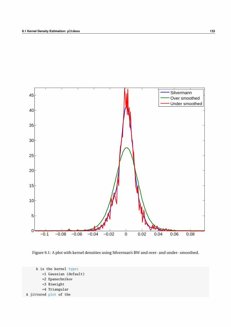
9.1 Kernel Density Estimation: pltdens 133
−0.1 −0.08 −0.06 −0.04 −0.02 0 0.02 0.04 0.06 0.080
5
10
15
20
25
30
35
40
45
SilvermannOver smoothedUnder smoothed
Figure 9.1: A plot with kernel densities using Silverman’s BW and over- and under- smoothed.
k is the kernel type:
=1 Gaussian (default)
=2 Epanechnikov
=3 Biweight
=4 Triangular
A jittered plot of the

134 Density Estimation
observations is shown below the density.
--------------------------------------------------
RETURNS:
h = the interval used
f = the density
y = the domain of support
plot(y,f) will produce a plot of the density
--------------------------------------------------
SEE ALSO hist, histo
--------------------------------------------------
9.2 Distributional Fit Testing 135
9.2 Distributional Fit Testing
9.2.1 Jarque-Bera Test: jarquebera
Jarque-Bera test for normality, defined as
(T − K )(
sk 2
6+(κ− 3)2
24
)where sk is the sample skewness and κ is the sample kurtosis.
9.2.1.1 Examples
% Jarque-Bera test on normal data
x = randn(100,1);
[statistic, pval] = jarquebera(x);
% Jarque-Bera test on regression errors
% where there were 4 regressors (4 mean parameters + 1 variance)
y=randn(100,1);x = randn(100,4); e = y - x*(x
[statistic, pval] = jarquebera(e, 5)
9.2.1.2 Required Inputs
[outputs] = jarquebera(DATA)
• DATA: T by 1 vector of data to be tested.
9.2.1.3 Optional Inputs
[outputs] = jarquebera(DATA,K,ALPHA)
• K: Degree of freedom adjustment. Default is 2.
• ALPHA: Size of the test to use. Default is 5%.
9.2.1.4 Outputs
[STATISTIC,PVAL,H] = jarquebera(inputs)
• STATISTIC: Jarque-Bera test statistic.
• PVAL: P-value evaluated using the asymptotic χ22 distribution.
• H: Logical indicating whether the test rejects at ALPHA.

136 Density Estimation
9.2.1.5 Comments
Computes the Jarque-Bera test for normality using the skewness and kurtosis to determine if a
distribution is normal.
USAGE:
[STATISTIC] = jarquebera(DATA)
[STATISTIC,PVAL,H] = jarquebera(DATA,K,ALPHA)
INPUTS:
DATA - A set of data to be tested for deviations from normality
K - [OPTIONAL] The number of dependant variables if any used in constructing the errors
(if omitted K=2)
ALPHA - [OPTIONAL] The level of the test used for the null of normality. Default is .05
OUTPUTS:
STATISTIC - A scalar representing the statistic
PVAL - A scalar pval of the null
H - A hypothesis dummy (0 for fail to reject the null of normality, 1 otherwise)
COMMENTS:
The data entered can be mean 0 or not. In either case the sample mean is subtracted and the
data are standardized by the sample standard deviation before computing the statistic .
EXAMPLES:
J-B test on normal data
x = randn(100,1);
[statistic, pval] = jarquebeta(x);
J-B test on regression errors where there were 4 regressors (4 mean parameters + 1 variance)
x = randn(100,1);
[statistic, pval] = jarquebeta(x, 5)
9.2 Distributional Fit Testing 137
9.2.2 Kolmogorov-Smirnov Test: kolmogorov
Kolmogorov-Smirnov test for correct unconditional distribution.
9.2.2.1 Examples
% Test data for uniformity
stat = kolmogorov(x)
% Test standard normal data
[stat,pval] = kolmogorov(x,[],’normcdf’)
% Test normal mean 1, standard deviation 2 data
[stat,pval] = kolmogorov(x,[],’normcdf’,1,2)
9.2.2.2 Required Inputs
[outputs] = kolmogorov(X)
• X: Data to be tested. X should have been transformed such that it is uniform (under the hypothesized
distribution).
9.2.2.3 Optional Inputs
[outputs] = kolmogorov(X,ALPHA,DIST,VARARGIN)
• ALPHA: Size of the test to use. Default is 5%.
• DIST: A string or function handle containing the name of a CDF to use to transform X to be uniform
(under the hypothesized distribution).
• VARARGIN: Optional arguments needed by DIST.
9.2.2.4 Outputs
[STAT,PVAL,H] = kolmogorov(inputs)
• STATISTIC: Kolmogorov-Smirnov test statistic.
• PVAL: P-value evaluated using a Monte Carlo distribution.
• H: Logical indicating whether the test rejects at ALPHA.

138 Density Estimation
9.2.2.5 Comments
Performs a Kolmogorov-Smirnov test that the data are from a specified distribution
USAGE:
[STAT,PVAL,H] = kolmogorov(X,ALPHA,DIST,VARARGIN)
INPUTS:
X - A set of random variable to be tested for distributional correctness
ALPHA - [OPTIONAL] The size for the test or use for computing H. 0.05 if not entered or
empty.
DIST - [OPTIONAL] A char string of the name of the CDF, i.e. ’normcdf’ for the normal,
’stdtcdf’ for standardized Student’s T, etc. If not provided or empty, data are
assumed to have a uniform distribution (i.e. that data have already been fed
through a probability integral transform)
VARARGIN - [OPTIONAL] Arguments passed to the CDF, such as the mean and variance for a normal
or a d.f. for T. The VARARGIN should be such that DIST(X,VARARGIN) is a valid
function with the correct inputs.
OUTPUTS:
STAT - The KS statistic
PVAL - The asymptotic probability of significance
H - 1 for reject the null that the distribution is correct, using the size provided (or
.05 if not), 0 otherwise
EXAMPLES:
Test data for uniformity
stat = kolmogorov(x);
Test standard normal data
[stat,pval] = kolmogorov(x,[],’normcdf’);
Test normal mean 1, standard deviation 2 data
[stat,pval] = kolmogorov(x,[],’normcdf’,1,2);
COMMENTS:
See also BERKOWITZ

9.2 Distributional Fit Testing 139
9.2.3 Berkowitz Test: berkowitz
Berkowitz (2001) test for correct fit in conditional density models.
9.2.3.1 Examples
% Test uniform data from a TS model
stat = berkowitz(x);
% Test standard normal data from a TS model
[stat,pval] = berkowitz(x,’TS’,[],’normcdf’);
% Test normal mean 1, standard deviation 2 data from a TS model
[stat,pval] = berkowitz(x,’TS’,[],’normcdf’,1,2);
9.2.3.2 Required Inputs
[outputs] = berkowitz(X)
• X: Data to be tested. X should have been transformed such that it is uniform (under the hypothesized
distribution).
9.2.3.3 Optional Inputs
[outputs] = berkowitz(X,TYPE,ALPHA,DIST,VARARGIN)
• TYPE: String either ’TS’ or ’CS’. Determines whether the test statistics looks at the AR(1) coefficient
(’TS’ does, ’CS’ does not). Default is ’TS’.
• ALPHA: Size of the test to use. Default is 5%.
• DIST: A string or function handle containing the name of a CDF to use to transform X to be uniform
(under the hypothesized distribution).
• VARARGIN: Optional arguments needed by DIST.
9.2.3.4 Outputs
[STAT,PVAL,H] = berkowitz(inputs)
• STATISTIC: Berkowitz test statistic.
• PVAL: P-value evaluated using the asymptotic χ2q distribution where q = 2 or q = 3, depending on
TYPE.
• H: Logical indicating whether the test rejects at ALPHA.

140 Density Estimation
9.2.3.5 Comments
Performs a Kolmogorov-Smirnov-like test using the Berkowitz transformation to a univariate normal
that the data are from a specified distribution.
USAGE:
[STAT,PVAL,H] = berkowitz(X,TYPE,ALPHA,DIST,VARARGIN)
INPUTS:
X - A set of random variable to be tested for distributional correctness
TYPE - [OPTIONAL] A char string, either ’CS’ if the data are cross-sectional or ’TS’ for
time series. The TS checks for autocorrelation in the prob integral transforms
while the CS does not. ’TS’ is the default value.
ALPHA - [OPTIONAL] The size for the test or use for computing H. 0.05 if not entered or
empty.
DIST - [OPTIONAL] A char string of the name of the CDF of X, i.e. ’normcdf’ for the normal,
’stdtcdf’ for standardized Studnet’s T, etc. If not provided or empty, data are
assumed to have a uniform distribution (i.e. that data have already been fed
through a probability integral transform)
VARARGIN - [OPTIONAL] Arguments passed to the CDF, such as the mean and variance for a normal
or a d.f. for T. The VARARGIN should be such that DIST(X,VARARGIN) is a valid
function with the correct inputs.
OUTPUTS:
STAT - The Berkowitz statistic computed as a likelihood ratio of normals
PVAL - The asymptotic probability of significance
H - 1 for reject the null that the distribution is correct using the size provided (or
.05 if not), 0 otherwise
EXAMPLES:
Test uniform data from a TS model
stat = berkowitz(x);
Test standard normal data from a TS model
[stat,pval] = berkowitz(x,’TS’,[],’normcdf’);
Test normal mean 1, standard deviation 2 data from a TS model
[stat,pval] = berkowitz(x,’TS’,[],’normcdf’,1,2);
COMMENTS:
See also KOLMOGOROV
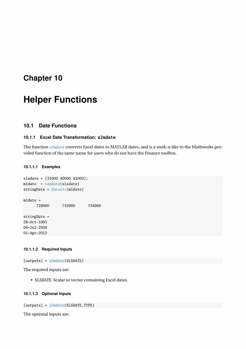
Chapter 10
Helper Functions
10.1 Date Functions
10.1.1 Excel Date Transformation: x2mdate
The function x2mdate converts Excel dates to MATLAB dates, and is a work-a-like to the Mathworks pro-
vided function of the same name for users who do not have the Finance toolbox.
10.1.1.1 Examples
xlsdate = [35000 40000 41000];
mldate = x2mdate(xlsdate)
stringDate = datestr(mldate)
mldate =
728960 733960 734960
stringDate =
28-Oct-1995
06-Jul-2009
01-Apr-2012
10.1.1.2 Required Inputs
[outputs] = x2mdate(XLSDATE)
The required inputs are:
• XLSDATE: Scalar or vector containing Excel dates.
10.1.1.3 Optional Inputs
[outputs] = x2mdate(XLSDATE,TYPE)
The optional inputs are:
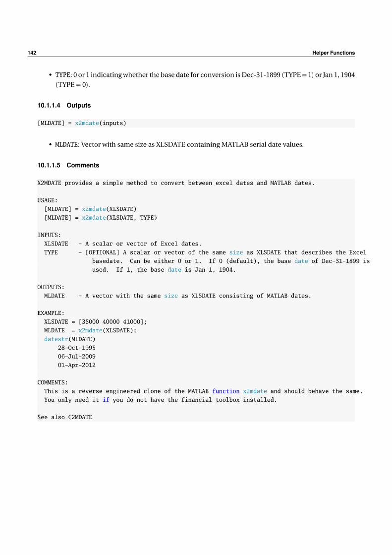
142 Helper Functions
• TYPE: 0 or 1 indicating whether the base date for conversion is Dec-31-1899 (TYPE= 1) or Jan 1, 1904
(TYPE = 0).
10.1.1.4 Outputs
[MLDATE] = x2mdate(inputs)
• MLDATE: Vector with same size as XLSDATE containing MATLAB serial date values.
10.1.1.5 Comments
X2MDATE provides a simple method to convert between excel dates and MATLAB dates.
USAGE:
[MLDATE] = x2mdate(XLSDATE)
[MLDATE] = x2mdate(XLSDATE, TYPE)
INPUTS:
XLSDATE - A scalar or vector of Excel dates.
TYPE - [OPTIONAL] A scalar or vector of the same size as XLSDATE that describes the Excel
basedate. Can be either 0 or 1. If 0 (default), the base date of Dec-31-1899 is
used. If 1, the base date is Jan 1, 1904.
OUTPUTS:
MLDATE - A vector with the same size as XLSDATE consisting of MATLAB dates.
EXAMPLE:
XLSDATE = [35000 40000 41000];
MLDATE = x2mdate(XLSDATE);
datestr(MLDATE)
28-Oct-1995
06-Jul-2009
01-Apr-2012
COMMENTS:
This is a reverse engineered clone of the MATLAB function x2mdate and should behave the same.
You only need it if you do not have the financial toolbox installed.
See also C2MDATE
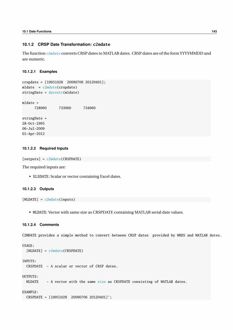
10.1 Date Functions 143
10.1.2 CRSP Date Transformation: c2mdate
The function c2mdate converts CRSP dates to MATLAB dates. CRSP dates are of the form YYYYMMDD and
are numeric.
10.1.2.1 Examples
crspdate = [19951028 20090706 20120401];
mldate = c2mdate(crspdate)
stringDate = datestr(mldate)
mldate =
728960 733960 734960
stringDate =
28-Oct-1995
06-Jul-2009
01-Apr-2012
10.1.2.2 Required Inputs
[outputs] = c2mdate(CRSPDATE)
The required inputs are:
• XLSDATE: Scalar or vector containing Excel dates.
10.1.2.3 Outputs
[MLDATE] = c2mdate(inputs)
• MLDATE: Vector with same size as CRSPDATE containing MATLAB serial date values.
10.1.2.4 Comments
C2MDATE provides a simple method to convert between CRSP dates provided by WRDS and MATLAB dates.
USAGE:
[MLDATE] = c2mdate(CRSPDATE)
INPUTS:
CRSPDATE - A scalar or vector of CRSP dates.
OUTPUTS:
MLDATE - A vector with the same size as CRSPDATE consisting of MATLAB dates.
EXAMPLE:
CRSPDATE = [19951028 20090706 20120401]’;

144 Helper Functions
MLDATE = c2mdate(CRSPDATE);
datestr(MLDATE)
28-Oct-1995
06-Jul-2009
01-Apr-2012
COMMENTS:
This is provided to make it easy to move between CRSP and MATLAB dates.
See also X2MDATE

Bibliography
Baxter, Marianne and Robert G King (Nov. 1999). “Measuring Business Cycles: Approximate Band-Pass
Filters For Economic Time Series”. In: The Review of Economics and Statistics 81.4, pp. 575–593.
Berkowitz, Jeremy (2001). “Testing density forecasts, with applications to risk management”. In: Journal
of Business & Economic Statistics 19, pp. 465–474.
Haan, Wouter den and Andrew T Levin (2000). Robust Covariance Estimation with Data-Dependent VAR
Prewhitening Order. Tech. rep. University of California – San Diego.
Hansen, Peter R, Asger Lunde, and Jason M Nason (Mar. 2005). “Model Confidence Sets for Forecasting
Models”.
Hansen, Peter Reinhard (Oct. 2005). “A Test for Superior Predictive Ability”. In: Journal of Business & Eco-
nomic Statistics 23.4, pp. 365–380.
Hodrick, Robert J and Edward C Prescott (Feb. 1997). “Postwar U.S. Business Cycles: An Empirical Inves-
tigation”. In: Journal of Money, Credit and Banking 29.1, pp. 1–16.
White, Halbert (Oct. 2000). Asymptotic Theory for Econometricians. Economic Theory, Econometrics, and
Mathematical Economics. Academic Press, p. 264.