M/G/1 queues and Busy Cycle Analysiscslui/CSC5420/lecture4.pdf · M=G=1 queues and Busy Cycle Analysis John C.S. Lui Department of Computer Science & Engineering The Chinese University

M/G/1 queues and Busy Cycle Analysis

John C.S. Lui

Department of Computer Science & EngineeringThe Chinese University of Hong Kong

www.cse.cuhk.edu.hk/∼cslui

John C.S. Lui (CUHK) Computer Systems Performance Evaluation 1 / 36

Outline

Outline

1 Renewal Theory

2 M/G/1


Renewal Theory

Another notation for transform

Given a discrete r.v G with gi = Prob[g = i]1 G(Z ) =

∑∞i=0 giZ i

2 E [Z G] =∑∞

i=0 Z iProb[g = i] =∑∞

i=0 Z igi Therefore,E [Z G] = G(Z )

Given a continuous r.v X with fX (x)1 F ∗

X(s) =

∫∞x=0 fX (x)e−sxdx

2 E [e−sX ] =∫∞

x=0 e−sx fX (x)dx


Renewal Theory

Residual Life

X0 Y

time1! 2! 3! n-1! n!

A2 A3A1 An-1 An

........

X

Interarrival time of bus is exponential w/ rate λ while hippie arrivesat an arbitrary instant in timeQuestion: How long must the hippie wait, on the average, till thebus comes along?


Renewal Theory

AnswerAnswer 1 : Because the average interarrival time is 1

λ , therefore 12λ

Answer 2 : Because of memoryless, it has to wait 1λ

General Result:

fX (x)dx = kxf (x)dx =xf (x)∫∞

0 xf (x)dx

fY (y) =1− F (y)∫∞0 xf (x)dx

F ∗(s) =1− F ∗(s)

m1

rn =mn+1

(n + 1)m1

Particularly, r1 = x2

2x


Renewal Theory

Derivation

P[x < X ≤ x + dx ] = fX (x)dx = kxf (x)dx∫ ∞x=0

fX (x)dx = k∫ ∞

x=0xf (x)dx ⇒ 1 = km1

Therefore,

fX (x) =1

m1xf (x)

fY (y) = ?

P[Y ≤ y |X = x ] =yx

P[y < Y ≤ y + dy , x < X ≤ x + dx ] =

(dyx

)(xf (x)

m1

)dx


Renewal Theory

continue:

fY (y)dy =

∫ ∞x=y

P[y < Y ≤ y + dy , x < X ≤ x + dx ]

=

∫ ∞x=y

(dyx

)(xf (x)

m1)dx =

1− F (y)

m1dy

fY (y) =1− F (y)

m1since f (y) =

dF (y)

dy

=1− F ∗(s)

sm1


M/G/1

M/G/1

A(t) = 1− e−λt t ≥ 0a(t) = λe−λt t ≥ 0b(t) = general

Describe the state[N(t),Xo(t)]

N(t): The no. of customers present at time tXo(t): Service time already received by the customer in service attime t (or remaining service time).Rather than using this approach, we use the method of theimbedded Markov Chain


M/G/1

Imbedded Markov Chain [N(t), Xo(t)]Select the "departure" points, we therefore eliminate Xo(t)Now N(t) is the no. of customers left behind by a departurecustomer.

1 For Poisson arrival: Pk (t) = Rk (t) for all time t . Therefore, pk = rk .2 If in any system (even it’s non-Markovian) where N(t) makes

discontinuous changes in size(plus or minus)one, then

rk = dk = Prob[departure leaves k customers behind]

Therefore, for M/G/1,pk = dk = rk


M/G/1

i-2 i-1 i i+1 i+2 j

α0

α2

α1

α3

α j-i+1

αk = Prob[k arrivals during the service of a customer]

P =

α0 α1 α2 α3 · · ·α0 α1 α2 α3 · · ·0 α0 α1 α2 · · ·0 0 α0 α1 · · ·0 0 0 α0 · · ·...

......

......

αk = P[v = k ] =

∫ ∞0

P[v = k |x = x ]b(x)dx =

∫ ∞0

(λx)k

k !e−λxb(x)dx

π = πP and∑πi = 1. Question: why not πQ = 0,

∑πi = 1?


M/G/1

The mean queue lengthWe have two cases.Case 1: qn+1 = qn − 1 + vn+1 for qn > 0

server

queue

Cn Cn+1

Cn Cn+1

Cn Cn+1

qn+1qn

vn+1

t

t


M/G/1

Case 2: qn+1 = vn+1 for qn = 0

server

queue

Cn Cn+1

Cn Cn+1

Cn Cn+1

qn+1qn

vn+1

t

t

=0

Let ∆k =

{1 for k = 1,2, . . .0 for k = 0

qn+1 = qn −∆qn + vn+1


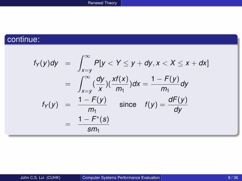
M/G/1

E [qn+1] = E [qn]− E [∆qn ] + E [vn+1]

Take the limit as n→∞, E [q] = E [q]− E [∆q] + E [v ]

We get,

E [∆q] = E [v ] = average no. of arrivals in a service time

On the other hand,

E [∆q] =∞∑

k=0

∆kP[q = k ]

= ∆0P[q = 0] + ∆1P[q = 1] + · · ·= P[q > 0]

Therefore E [∆q] = P[q > 0]. Since we are dealing with singleserver, it is also equal to P[busy system]=ρ = λ/mu = λx .Therefore,

E [v ] = ρ


M/G/1

Since we have

qn+1 = qn −∆qn + vn+1

q2n+1 = q2

n + ∆2qn + v2

n+1 − 2qn∆qn + 2qnvn+1 − 2∆qnvn+1

Note that : (∆qn )2 = ∆qn and qn∆qn = qn

limn→∞

E [q2n+1] = lim

n→∞{E [q2

n ] + E [∆2qn ] + E [v2

n+1]−

2E [qn] + 2E [qnvn+1]− 2E [∆qnvn+1]}0 = E [∆q] + E [v2]− 2E [q] + 2E [q]E [v ]− 2E [∆q]E [v ]

E [q] = ρ+E [v2]− E [v ]

2(1− ρ)

Now the remaining question is how to find E [v2].


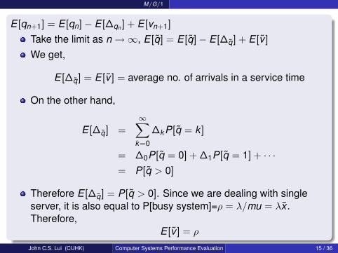
M/G/1

Let V (Z ) =∑∞

k=0 P[v = k ]Z k

V (Z ) =∞∑

k=0

∫ ∞0

(λx)k

k !e−λxb(x)dxZ k

=

∫ ∞0

e−λx

( ∞∑k=0

(λxZ )k

k !

)b(x)dx

=

∫ ∞0

e−λxeλxZ b(x)dx

=

∫ ∞0

e−(λ−λZ )xb(x)dx

Look at B∗(s) =∫∞

0 e−sxb(x)dx . Therefore,

V (Z ) = B∗(λ− λZ )


M/G/1

From this, we can get E [v ],E [v2], . . .

dV (Z )

dZ=

dB∗(λ− λZ )

dZ=

dB∗(λ− λZ )

d(λ− λZ )• d(λ− λZ )

dZ

= −λdB∗(y)

dydV (Z )

dZ

∣∣∣Z=1

= −λdB∗(y)dy

∣∣∣y=0

= +λx = ρ


M/G/1

d2V (Z )dZ 2 = v2 − v , since V (Z ) = B∗(λ− λZ )

d2V (Z )

dZ 2 =d

dZ[−λdB∗(y)

dy] = −λd2B∗(y)

dy2dydZ

d2V (Z )

dZ 2 |Z=1 = λ2 dB2∗(y)

dy2 |y=0 = λ2B∗(2)(0)

v2 − v = λ2x2 ⇒ v2 = v + λ2x2

Go back, since

E [q] = ρ+E [v2]− E [v ]

2(1− ρ)

E [q] = ρ+λ2x2

2(1− ρ)= ρ+ ρ2 (1 + C2

b)

2(1− ρ)

This is the famous Pollaczek - Khinchin Mean Value Formula.John C.S. Lui (CUHK) Computer Systems Performance Evaluation 19 / 36

M/G/1

For M/M/1, b(x) = µe−µx , x = 1µ ; x2 = 2

µ2

q = ρ+λ2x2

2(1− ρ)= ρ+

2λ2

µ2

2(1− ρ)= ρ+ ρ2 2

2(1− ρ)

q =ρ

1− ρ= N in M/M/1

For M/D/1, x = x ; x2 = x2

q = ρ+ ρ2 12(1− ρ)

=ρ

1− ρ− ρ2

2(1− ρ)

→ It’s less than M/M/1 !For M/H2/1, let b(x) = 1

4λe−λx + 34(2λ)e−2λx ; x = 5

8λ ; x2 = 5664λ2

q = ρ+5664

2(1− ρ)where ρ = λx =

58

; q = 1.79


M/G/1

Distribution of Number in the System

qn+1 = qn −∆qn + vn+1

Z qn+1 = Z qn−∆qn +vn+1

E [Z qn+1 ] = E [Z qn−∆qn +vn+1 ] = E [Z qn−∆qn · Z vn+1 ]

Taking limit as n→∞

Q(Z ) = E [Z q−∆q ] · E [Z v ] = E [Z q−∆q ]V (Z )→ (1)

E [Z q−∆q ] = Z 0−0Prob[q = 0] +∞∑

k=1

Z k−1Prob[q = k ]

= Z 0Prob[q = 0] +1Z

[Q(Z )− P[q = 0]]

= Prob[q = 0] +1Z

[Q(Z )− P[q = 0]]


M/G/1

ContinuePutting them together, we have:

Q(Z ) = V (Z )(Prob[q = 0] +1Z

[Q(Z )− P[q = 0]])

But P[q = 0] = 1− ρ, we have:

Q(Z ) = V (Z )[(1− ρ)(1− 1

Z )

1− V (Z )Z

] = B∗(λ− λZ )[(1− ρ)(1− Z )

B∗(λ− λZ )− Z]

This is the famous P-K Transform equation.


M/G/1

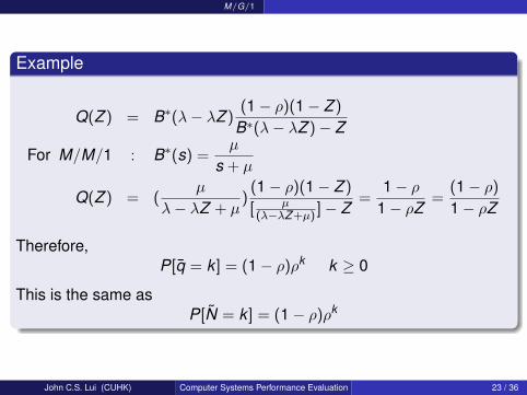
Example

Q(Z ) = B∗(λ− λZ )(1− ρ)(1− Z )

B∗(λ− λZ )− Z

For M/M/1 : B∗(s) =µ

s + µ

Q(Z ) = (µ

λ− λZ + µ)

(1− ρ)(1− Z )

[ µ(λ−λZ+µ) ]− Z

=1− ρ

1− ρZ=

(1− ρ)

1− ρZ

Therefore,P[q = k ] = (1− ρ)ρk k ≥ 0

This is the same asP[N = k ] = (1− ρ)ρk


M/G/1

Continue

Q(Z ) = B∗(λ− λZ )(1− ρ)(1− Z )

B∗(λ− λZ )− Z

For M/H2/1 : B∗(s) =14

λ

s + λ+

34

2λs + 2λ

=7λs + 8λ2

4(s + λ)(s + 2λ)

Q(Z ) =(1− ρ)(1− z)[8 + 7(1− z)]

8 + 7(1− z)− 4z(2− z)(3− z)

=(1− ρ)[1− 7

15z]

[1− 25z][1− 2

3z]= (1− ρ)

[14

1− 25z

+34

1− 23z

]

Where ρ = λx = 58

Pk = Prob[q = k ] =332

(25

)k

+9

32

(23

)k

k = 0,1,2, · · ·


M/G/1

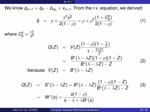
We know qn+1 = qn −∆qn + vn+1. From the r.v. equation, we derived:

q = ρ+λ2x2

2(1− ρ)= ρ+ ρ2 (1 + C2

b)

2(1− ρ), (1)

where C2b =

σ2b

x2

Q(Z ) = V (Z )(1− ρ)(1− 1

Z )

1− V (Z )Z

=B∗(λ− λZ )(1− ρ)(1− Z )

B∗(λ− λZ )− Z(2)

because V (Z ) = B∗(λ− λZ )

Q(Z ) = S∗(λ− λZ ) = B∗(λ− λZ )(1− ρ)(1− Z )

B∗(λ− λZ )− Z(3)

→ W ∗(s) =s(1− ρ)

s − λ+ λB∗(s)


M/G/1

Distribution of Waiting Time

Cn

Cn

Cn

xn

vn Cn

Cn

Cn

xn

wn

q n

V ∗(z) = B∗(λ− λz) Q(z) = S∗(λ− λz)

S∗(λ− λZ ) = B∗(λ− λZ )(1− ρ)(1− Z )

B∗(λ− λZ )− Z

Let s = λ− λz, then z = 1− sλ

S∗(s) = B∗(s)s(1− ρ)

s − λ+ λB∗(s)What is W ∗(s)?


M/G/1

For M/M/1,

S∗(s) = B∗(s)s(1− ρ)

s − λ+ λB∗(s)B∗(s) =

µ

s + µ

= [µ

s + µ][

s(1− ρ)

s − λ+ λ µs+µ

]

= [µ][s(1− ρ)

s2 + sµ− sλ]

=sµ(1− ρ)

s[s + µ− λ]=

µ(1− ρ)

s + µ− λ

=µ(1− ρ)

s + µ(1− ρ)

s(y) = µ(1− ρ)e−µ(1−ρ)y y ≥ 0S(y) = 1− e−µ(1−ρ)y y ≥ 0


M/G/1

W ∗(s) =s(1− ρ)

s − λ+ λ µs+µ

=s(1− ρ)(s + µ)

s2 + sµ− sλ

=s(1− ρ)(s + µ)

s[s + µ− λ]=

(1− ρ)(s + µ)

s + µ− λ

= (1− ρ) +λ(1− ρ)

s + µ− λ= (1− ρ) +

λ(1− ρ)

s + µ(1− ρ)

w(y) = (1− ρ)µ0(y) + λ(1− ρ)e−µ(1−ρ)y y ≥ 0W (y) = 1− ρe−µ(1−ρ)y y ≥ 0

1

1−ρ


M/G/1

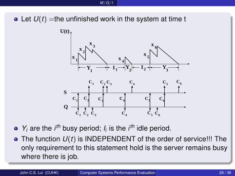
Let U(t) =the unfinished work in the system at time t

U(t)

Y1

I 1

x1

x2

x3

x4

x5

x6

Y2

I 2 Y3

S

QC1

C1

C1

C2

C2

C2

C3

C3

C3

C4

C4

C4

C5

C5

C5

C6

C6

C6

Yi are the i th busy period; Ii is the i th idle period.The function U(t) is INDEPENDENT of the order of service!!! Theonly requirement to this statement hold is the server remains busywhere there is job.


M/G/1

For M/G/1

A(t) = P[tn ≤ t ] = 1− e−λt t ≥ 0B∗(x) ⇔ P[Xn ≤ x ]

Let

F (y) = P[In ≤ y ]

= idle-period distributionG(y) = P[Yn ≤ y ]

= busy-period distribution

F (y) = 1− e−λt t ≥ 0

G(y) is not that trivial! Well, thanks to Takacs, he came to therescue.


M/G/1

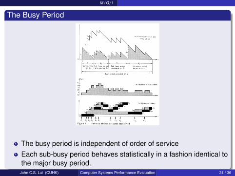
The Busy Period

The busy period is independent of order of serviceEach sub-busy period behaves statistically in a fashion identical tothe major busy period.


M/G/1

The duration of busy period Y , is the sum of 1 + v randomvariables where

Y = x1 + Xv + · · ·+ X1

where x1 is the service time of C1, Xv is the (v + 1)th sub-busyperiod and v is the r.v. of the number of arrival during the serviceof C1.Let G(y) = P[Y ≤ y ] and G∗(s) =

∫∞0 e−sydG(y) = E [e−sY ]

E [e−sY |x1 = x , v = k ] = E [e−s(x+Xk+1+Xk +···+X2)]

= E [e−sx ]E [e−sXk+1 ]E [e−sXk ] · ·E [e−sX2 ]

= e−sx [G∗(s)]k

E [e−sY |x1 = x ] =∞∑

k=0

E [e−sY |x1 = x , v = k ]P[v = k ]


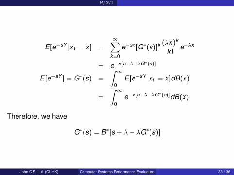
M/G/1

E [e−sY |x1 = x ] =∞∑

k=0

e−sx [G∗(s)]k(λx)k

k !e−λx

= e−x [s+λ−λG∗(s)]

E [e−sY ] = G∗(s) =

∫ ∞0

E [e−sY |x1 = x ]dB(x)

=

∫ ∞0

e−x [s+λ−λG∗(s)]dB(x)

Therefore, we have

G∗(s) = B∗[s + λ− λG∗(s)]


M/G/1

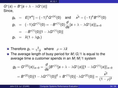
G∗(s) = B∗[s + λ− λG∗(s)]Since,

gk = E [Y k ] = (−1)kG∗(k)(0) and xk = (−1)kB∗(k)(0)

g1 = (−1)G∗(1)(0) = −B∗(1)(0)dds

[s + λ− λG∗(s)]|s=0

= −B∗(1)(0)[1− λG∗(1)(0)]

g1 = x(1 + λg1)

Therefore g1 = x1−p where ρ = λx

The average length of busy period for M/G/1 is equal to theaverage time a customer spends in an M/M/1 system

g2 = G∗(2)(s)|s=0 =dds

[B∗(1)[s + λ− λG∗(s)][1− λG∗(1)(s)]|s=0

= B∗(2)(0)[1− λG∗(1)(0)]2 + B∗(1)(0)[−λG∗(2)(0)] =x2

(1− ρ)3


M/G/1

The number of customers served in a busy periodLet Nbp = r.v. of no. of customers served in a busy period.

fn = Prob[Nbp = n]

F (Z ) = E [Z Nbp ] =∞∑

n=1

fnZ n

E [Z Nbp |v = k ] = E [Z 1+Mk +Mk−1+···+M1 ]

(where Mi = no. of customers served in the i th sub-busy period)

E [Z Nbp |v = k ] = E [Z ]E [Z Mk ] · · ·E [Z M1 ] = E [Z ](E [Z Mi ])k

= Z [F (Z )]k


M/G/1

Continue

F (Z ) =∞∑

k=0

E [Z Nbp |v = k ]P[v = k ]

=∞∑

k=0

Z [F (Z )]kP[v = k ]

= ZV [F (Z )]

⇒ F (Z ) = ZB∗(λ− λF (Z ))


Documents

M/G/1 queues and Busy Cycle Analysiscslui/CSC5420/lecture4.pdf · M=G=1 queues and Busy Cycle Analysis John C.S. Lui Department of Computer Science & Engineering The Chinese University